The Integer Linear Programming Inference Cookbook

Abstract

Over the years, integer linear programs have been employed to model inference in many natural language processing problems. This survey is meant to guide the reader through the process of framing a new inference problem as an instance of an integer linear program and is structured as a collection of recipes. At the end, we will see two worked examples to illustrate the use of these recipes.

1 Introduction

Effective decision-making requires the use of knowledge. This has been a clear, and long-standing principle in AI research, as reflected, for example, in the seminal early work on knowledge and AI—summarized by Brachman and Levesque (1985)—and the thriving Knowledge Representation and Reasoning and the Uncertainty in AI communities. However, the message has been somewhat diluted as data-driven statistical learning has become increasingly pervasive across AI. Nevertheless, the idea that reasoning and learning need to work together (Khardon and Roth, 1996; Roth, 1996) and that knowledge representation is a crucial bridge between them has not been lost.

One area where the link between learning, representation, and reasoning has been shown to be essential and has been studied extensively is Natural Language Processing (NLP), and in particular, the area of Structured Output Prediction within NLP. In structured problems, there is a need to assign values to multiple random variables that are interrelated. Examples include extracting multiple relations among entities in a document, where a the two arguments for a relation such as born-in cannot refer to people, or co-reference resolution, where gender agreement must be maintained when determining that a specific pronoun refers to a given entity. In these, and many other such problems, it is natural to represent knowledge as Boolean functions over propositional variables. These functions would express knowledge, for example, of the form “if the relation between two entities is born-in, then its arguments must be a person and a location” (formalized as functions such as $x_{i}\rightarrow x_{j}\lor x_{k}$, or exactly one of $x_{1},x_{2},\ldots x_{k}$ can be true). These functions serve to constrain the feasible solutions to the inference problem and open the possibility to model the global decision problem as a constrained optimization problem.

An influential, and as we will see, also natural formalism for the decision problem is to frame it as an Integer Linear Program (ILP). This approach was first employed in NLP in the context of information extraction and machine translation (Roth and Yih, 2004; Germann et al., 2004; Roth and Yih, 2005) The objective function for the integer program in question is typically learned, and could be viewed as proposing, for each variable of interest, a distribution over the values it can take. The final assignment to these variables is then determined by maximizing the objective, subject to knowledge constraints, such as the ones described above. The ability to decouple the modeling of a problem and the knowledge needed to support inference, from learning the models is one reason that has made the ILP formulation a popular one in NLP. Over the years, ILPs have been employed to model inference in many natural language processing (NLP) problems—information extraction (Roth and Yih, 2004; Choi et al., 2006; Denis and Muller, 2011; Berant et al., 2014), decoding in machine translation (Germann et al., 2004), semantic role labeling (Punyakanok et al., 2008; Srikumar and Roth, 2011), dependency parsing (Riedel and Clarke, 2006; Martins et al., 2009), coreference resolution (Denis and Baldridge, 2009), sentence compression (Clarke and Lapata, 2008; Thadani and McKeown, 2013), inferring alignments (Goldwasser and Roth, 2008; Chang et al., 2010; Li and Srikumar, 2016), summarization (Woodsend and Lapata, 2012), supertagging (Ravi et al., 2010), common sense reasoning (Roy and Roth, 2015; Goldwasser and Zhang, 2016), and many others. It is important to point out that these examples include both cases where the computational aspects of inference were handled by powerful off-the-shelf solvers such as Express-MP or Gurobi, and those where approximate methods were designed for inference.

The integer linear programming formalism is both expressive and easy to use for representing and reasoning with knowledge for two reasons. First, every MAP inference problem with discrete variables can be represented as a linear objective (Roth and Yih, 2007), making ILP a natural formalism for such problems. Second, all Boolean functions can be compiled into a set of linear inequalities, to be used as constraints in the ILP formulation.

This tutorial-style survey paper focuses on this second point, and is meant to guide the reader through the process of framing a new inference problem as an instance of an integer linear program. It is structured as a collection of commonly used recipes, and at the end, we will see two worked examples to illustrate the use of these recipes.

To simplify discourse, we will make two assumptions. First, we will assume that we have all the scoring functions needed to write the objective function. Second, we will primarily focus on the process of writing down the inference problems, not solving them. It is important to separate the declaration of a problem from its solution; this article concerns the former. We could solve inference problems using off-the-shelf black box solvers, general heuristics, or specially crafted algorithms tailored to the problem at hand.

A final note before we get started: While the motivating examples used in this paper are drawn from natural language processing, the techniques for converting Boolean expressions into linear inequalities that are discussed here are applicable more broadly. As a result, the next few sections are written without a specific domain in mind, but the worked examples that follow are grounded in NLP tasks.

2 Notation and Preliminaries

To start off, let us first see the notation that will be used through this survey.

Decision variables.

Our goal is to collectively make a set of possibly interacting decisions. We will refer to individual Boolean decisions using the symbol $y$ with subscripts. Usually, the decisions in the subscripts deal with assigning labels to inputs. For example, the decision that the $i^{th}$ label is A will be represented as $y_{{i:{\tt A}}}$. For brevity, if the label $A$ is the constant true, we will write $y_{{i}}$ to denote $y_{{i:{\tt true}}}$.

We can map from the space of Boolean decisions (i.e., predicates) to integers using the Iverson bracket (Iverson, 1962). The Iverson bracket for a predicate $y$, denoted by $\left[y\right]$, is defined as

$$\left[y\right]=\begin{cases}1&\mbox{if }y\mbox{ is {\tt true}}\\ 0&\mbox{if }y\mbox{ is {\tt false}}.\end{cases}$$ (1)

In other words, it maps true to $1$ and false to $0$. As Knuth (1992) points out, the Iverson bracket is a notational convenience that vastly simplifies mathematical exposition. Here, we will assume the implicit existence of the Iverson bracket to translate false and true to $0$ and $1$ respectively. This implicit notational device will allow us to reason about Boolean variables like $y$ as if they were integers.

Each decision $y_{{i}}$ is associated with a score $c_{{i}}$. We will assume the convention that we prefer decisions whose scores are larger. Importantly, in this survey, we will not concern ourselves with where the scores originate; the scoring function could have been learned in the past, or the inference could be situated within the context of a learning algorithm that estimates the scoring function, or perhaps the scores were manually set using domain knowledge. Furthermore, we do not make any assumptions about the nature of the scores—while they could represent log probabilities that the corresponding variable is true, we do not assume that they are probabilities in the formal sense; we merely require that variable assignments that are associated with a higher total score are preferable.

Finally, we will use the boldface symbol ${{\bf y}}$ to denote a vector of decision variables and the boldface ${{\bf c}}$ to denote the vector of coefficients that score the decision variables in ${{\bf y}}$.

Integer linear programs.

The goal of inference is to assign values to the decision variables such that their total score is maximized. We will formalize this task as an integer linear program (ILP). To define the integer linear program, we need to specify a linear objective function and a collection of linear constraints that characterize the set of valid decisions. In general, we can write the inference problem as

$$\max_{{{\bf y}}} \sum\limits_{i}c_{{i}}y_{{i}}$$ (2)

s.t. $${{\bf y}}\in\mathcal{Y},$$ (3)

$$y_{{i}}\in\{0,1\}.$$ (4)

Here, $\mathcal{Y}$ denotes a set of legal assignments to the inference variables. The actual definition of this set in the form of linear inequalities is dependent on the problem and the subsequent sections are devoted to recipes for constructing this set.

Of course, even the definition of the inference variables is a problem-specific design choice. The inference variables in the objective function are constrained to be zero or one. Thus, our problem is an instance of a $0$-$1$ integer linear program. The linear objective (2) ensures that only the coefficients for variables that are assigned to true (or equivalently, to 1 via the Iverson bracket) will count towards the total score. While not explicitly stated in the formulation above, we can also add additional auxiliary discrete or real valued inference variables to allow us to state the problems in an easy way or to facilitate solving them.

Integer and mixed-integer programming is well studied in the combinatorial optimization literature. An overview of their computational properties is beyond the scope of this survey and the reader should refer to textbooks that cover this topic (Papadimitriou and Steiglitz, 1982; Schrijver, 1998, for example). For our purposes, we should bear in mind that, in general, integer programming is an NP-hard problem. Indeed, $0$-$1$ integer programming was one of Karp’s 21 NP-complete problems (Karp, 1972). Thus, while the techniques described in this tutorial provide the tools to encode our problem as an integer program, we should be aware that we may end up with a problem formulation that is intractable. For certain NLP problems such as semantic role labeling (Punyakanok et al., 2008, for example), we can show that certain ways to model the problem leads to inference formulations that are intractable in the worst case. Yet, curiously, in practice, off-the-shelf solvers seem to solve them quite fast! Indeed, the same problem could be encoded in different ways, one of which can be solved efficiently while another is not. One example of this situation is the task of graph-based dependency parsing. The ILP encoding of Riedel and Clarke (2006) required a specialized cutting-plane method, while the flow-inspired encoding of Martins et al. (2009) was more efficiently solvable.

3 Basic Operators: Logical Functions

In this section, we will introduce the basic building blocks needed to convert Boolean expressions into a set of linear inequalities. For now, we will only use $0$-$1$ decision variables as described in §2 without any auxiliary real-valued variables. Using only the techniques described in this section, we should be able to write any Boolean expression as a set of linear inequalities.

3.1 Variables and their Negations

Recall that each variable $y$ in the $0$-$1$ ILP corresponds to a Boolean decision. A natural first constraint may seek to enforce a certain set of decisions, or equivalently, enforce their logical conjunction. This gives us our first recipe.

Constraint 1: Forcing the conjunction of decisions $y_{{1}},y_{{2}},\ldots,y_{{n}}$ to be true. That is, $y_{{1}}\land y_{{2}}\land\cdots\land y_{{n}}$.

$$\sum\limits_{i=1}^{n}y_{{i}}=n.$$

Since the decision variables can only be $0$ or $1$, the sum in the constraint counts the number of decisions enforced. With $n$ variables, this sum can be $n$ if, and only if, each one of them takes the value $1$.

Handling negations.

Setting a variable $y$ to false  is equivalent to setting $1-y$ to true. This observation gives us a general strategy to deal with negations: Suppose a variable $y$ is negated in a Boolean expression. While converting this expression into a linear inequality (using one of the recipes in this survey), we will replace occurrences of $y$ in the inequality with $1-y$. For example, the constraint $\neg y$ would become $1-y=1$ (or $y=0$). Applying this strategy to the above constraint gives us a second constraint that forbids a collection of $n$ decisions from being true.

Constraint 2: Forbidding all the decisions $y_{{1}},y_{{2}},\ldots,y_{{n}}$ from being true. That is, $\neg y_{{1}}\wedge\neg y_{{2}}\wedge\cdots\wedge\neg y_{{n}}$.

$$\sum\limits_{i=1}^{n}y_{{i}}=0.$$

The need to force decision variables to be either true or false arises when we wish to unconditionally enforce some external knowledge about the prediction.

Example 1.

Suppose we know the ground truth assignments for a subset of our decision variables and we wish to ascertain the best assignment to the other variables according to our model. We could do so by forcing the known variables to their values. Such an approach could be useful for training models with partial supervision over structures.

Example 2 (Testing inference formulations).

Another use case for the above constraint recipes is that it offers a way to check if our inference formulation for a problem is correct. Suppose we have a labeled data set that maps inputs ${\bf x}$ (e.g., sentences) to outputs ${\bf y}$ (e.g., labeled graphs) and we have framed the problem of predicting these outputs as an ILP.

One way to test whether our problem formulation (as defined by our constraints) is meaningful is to add additional constraints that clamp the decision variables to their ground truth labels in a training set. If the resulting ILP is infeasible for any example, we know that the rest of our constraints do not accurately reflect the training data. Of course, we may choose not to correct this inconsistency with the data, but that is a modeling choice.

3.2 Disjunctions and their Variants

An important building block in our endeavor is the disjunction. Suppose we have a collection of decision variables and we require that at least one of them should hold. Using the Iverson notation naturally gives us the constraint formulation below.

Constraint 3: Disjunction of $y_{{1}},y_{{2}},\ldots,y_{{n}}$. That is, $y_{{1}}\vee y_{{2}}\vee\cdots\vee y_{{n}}$.

$$\sum\limits_{i=1}^{n}y_{{i}}\geq 1$$

Note that this constraint can incorporate negations using the construction from §3.1, as in the following example.

Example 3.

If we want to impose the constraint $\neg y_{{1}}\vee\neg y_{{2}}\vee\neg y_{{3}}$, we need to use $1-y_{{1}}$, $1-y_{{2}}$ and $1-y_{{3}}$ in the recipe above. This gives us

$$1-y_{{1}}+1-y_{{2}}+1-y_{{3}}\geq 1,$$

that is, $$y_{{1}}+y_{{2}}+y_{{3}}\leq 2.$$

There are several variations on this theme. Sometimes, we may require that the number of true assignments should be at least, or at most, or exactly equal to some number $k$. These counting quantifiers or cardinality quantifiers generalize both conjunctions and disjunctions of decisions. A conjunction of $n$ variables demands that the number of true assignments should be equal to $n$; their disjunction demands that at least one of the variables involved should be true.

Constraint 4: At least, at most or exactly $k$ true assignments among $y_{{1}},y_{{2}},\ldots,y_{{n}}$.

At least $$k \sum\limits_{i=1}^{n}y_{{i}}\geq k$$:

At most $$k \sum\limits_{i=1}^{n}y_{{i}}\leq k$$:

Exactly $$k \sum\limits_{i=1}^{n}y_{{i}}=k.$$:

The use of counting quantifiers does not increase the expressive power over logical expressions. They merely serve as a syntactic shorthand for much larger Boolean expressions. For example, if we wish to state that exactly two of the three variables $y_{{1}}$, $y_{{2}}$ and $y_{{3}}$ are true, we can encode it using the following expression:

$$\left(y_{{1}}\land y_{{2}}\land\neg y_{{3}}\right)\lor\left(y_{{1}}\land\neg y_{{2}}\land y_{{3}}\right)\lor\left(\neg y_{{1}}\land y_{{2}}\land y_{{3}}\right)$$

An important (that is, frequently applicable) special case of counting quantifiers is uniqueness quantification, where we require exactly one of a collection of decisions to hold. While the corresponding linear constraint is clearly easy to write using what we have seen above, uniqueness constraints are important enough to merit stating explicitly.

Constraint 5: Unique assignment among $y_{{1}},y_{{2}},\ldots,y_{{n}}$. That is, $\exists!~{}y_{{i}}$.

$$\sum\limits_{i=1}^{n}y_{{i}}=1.$$

As an aside, this constraint is identical to the logical XOR if we have exactly two variables (i.e., their parity is one when the constraint holds), but not when the number of variables is more. For example, with three variables, if all of them are assigned to true, their parity is one, but the above constraint is not satisfied.

Example 4 (Multiclass classification).

The linear constraint templates described in this section find wide applicability. The simplest (albeit unwieldy) application uses the unique label constraint to formally define multiclass classification. Suppose we have inputs that are to be assigned one of $n$ labels $\{{\tt l_{1}},{\tt l_{2}},\ldots,{\tt l_{n}}\}$. We can write this prediction problem as an integer linear program as follows:

$$\max_{{{\bf y}}} \sum\limits_{i=1}^{n}c_{{\mbox{\footnotesize label}:{\tt l_{i}}}}\cdot y_{{\mbox{\footnotesize label}:{\tt l_{i}}}}$$

such that $$\sum\limits_{i=1}^{n}y_{{\mbox{\footnotesize label}:{\tt l_{i}}}}=1,$$

$$y_{{\mbox{\footnotesize label}:{\tt l_{i}}}}\in\{0,1\}.$$

We have $n$ decision variables, each corresponding to one of the possible label assignments. The decision of choosing the label ${\tt l_{i}}$ is scored in the objective function by a score $c_{{\mbox{\footnotesize label}:{\tt l_{i}}}}$. The goal of inference is to find the score maximizing assignment of these decision variables. The constraint mandates that exactly one of the inference outcomes is allowed, thus ensuring that the label that maximizes the score is chosen.

The above example merely illustrates the use of the unique label constraint. While inference for multiclass classification can be written in this form, it is important to note that it is unwise to use a black box ILP solver to solve it; simply enumerating the labels and picking the highest scoring one suffices. This example highlights the difference between framing a problem as an integer linear program and solving it as one. While multiclass classification can clearly be framed as an ILP, solving it as one is not a good idea.

However, the multiclass as an ILP construction is a key building block for defining larger structured outputs. A commonly seen inference situation requires us to a unique label to each of a collection of categorical random variables, subject to other constraints that define the interactions between them. In such a situation, each categorical random variable will invoke the multiclass as an ILP construction.

3.3 A recipe for Boolean expressions

In §3.1 and §3.2, we saw recipes for writing Boolean variables, their negations, conjunctions and disjunctions as linear inequalities. With the full complement of operators, we can convert any constraint represented as a Boolean expression into a collection of linear inequalities using the following procedure:

1. Convert the Boolean expression into its conjunctive normal form (CNF) using De Morgan’s laws and the distributive property, or by introducing new variables and using the Tseitin transformation (Tseitin, 1983).

2. Recall that a CNF is a conjunction of disjunctive clauses. Express each clause in the CNF (a disjunction) as a linear inequality.

Let us work through this procedure with two examples. In both examples, we will not worry about the objective function of the ILP and only deal with converting Boolean expressions into linear constraints.

Example 5.

Suppose we have three Boolean variables $y_{{1}}$, $y_{{2}}$ and $y_{{3}}$ and our goal is to convert the following Boolean expression into linear inequalities:

$$\left(y_{{1}}\wedge\neg y_{{2}}\right)\vee\left(y_{{1}}\wedge\neg y_{{3}}\right)$$

The first step, according to the recipe above, is to convert this into its equivalent conjunctive normal form:

$$y_{{1}}\wedge\left(\neg y_{{2}}\vee\neg y_{{3}}\right).$$

Now, we have two clauses, each of which will become a linear constraint. Using the templates we have seen so far and simplifying, we get the following linear constraints:

$$y_{{1}}=1,$$

$$y_{{2}}+y_{{3}}\leq 1.$$

Example 6.

Suppose we have three decision variables $y_{{1}},y_{{2}}$ and $y_{{3}}$ and we wish to enforce the constraint that either all of them should be true or all of them should be false. The constraint can be naturally stated as:

$$\left(y_{{1}}\wedge y_{{2}}\wedge y_{{3}}\right)\vee\left(\neg y_{{1}}\wedge\neg y_{{2}}\wedge\neg y_{{3}}\right).$$

To express the constraint as a set of linear inequalities, let us first write down its conjunctive normal form:

$$\left(y_{{1}}\vee\neg y_{{2}}\right)\wedge\left(y_{{1}}\vee\neg y_{{3}}\right)\wedge\left(y_{{2}}\vee\neg y_{{1}}\right)\wedge\left(y_{{2}}\vee\neg y_{{3}}\right)\wedge\left(y_{{3}}\vee\neg y_{{1}}\right)\wedge\left(y_{{3}}\vee\neg y_{{2}}\right).$$

Now, we can convert each disjunctive clause in the CNF form to a different linear constraint following the templates we have seen before. After simplification, we get the following linear system that defines the feasible set of assignments:

$$y_{{1}}-y_{{2}}\geq 0,$$

$$y_{{1}}-y_{{3}}\geq 0,$$

$$y_{{2}}-y_{{1}}\geq 0,$$

$$y_{{2}}-y_{{3}}\geq 0,$$

$$y_{{3}}-y_{{1}}\geq 0,$$

$$y_{{3}}-y_{{2}}\geq 0.$$

The procedure provides a systematic approach for converting Boolean constraints (which are easier to state) to linear inequalities (allowing us to use industrial strength solvers for probabilistic inference). Indeed, the recipe is the approach suggested by Rizzolo and Roth (2007) and Rizzolo (2012) for learning based programming. However, if applied naïvely, this methodical approach can present us with difficulties with respect to the number of linear constraints generated.

Consider the final set of inequalities obtained in Example 6 above. While we could leave the linear system as it is, the system of equations implies that $y_{{1}}=y_{{2}}=y_{{3}}$, as does the logical expression that we started with. This example illustrates an important deficiency of the systematic approach for converting logical formulae into linear inequalities. While the method is sound and complete, it can lead to a much larger set of constraints than necessary. We will see in §4 that such “improperly” encoded constraints can slow down inference.

One way to address such a blowup in the number of constraints is to identify special cases that represent frequently seen inference situations and lead to large number of constraints, and try to find more efficient conversion techniques for them. The following sections enumerate such special cases, starting with implications (§4) and moving on to combinatorial structures (§5).

4 Simple and Complex Logical Implications

The first special case of constraints we will encounter are conditional forms. At first, we will simply convert the implications into disjunctions and use the disjunction templates from §3. Then, in §4.2, we will exploit the fact that our inference variables can only be $0$ or $1$ to reduce the number of constraints.

4.1 Simple Conditional Forms

First, let us consider the simplest implication constraint: $y_{{1}}\rightarrow y_{{2}}$. Clearly, this is equivalent to the disjunction $\neg y_{{1}}\vee y_{{2}}$ and we can convert it to the constraint $-y_{{1}}+y_{{2}}\geq 0$. We can generalize this to a conditional form with a conjunctive antecedent and a disjunctive consequent:

$$\bigwedge\limits_{i=1}^{m}y_{{l_{i}}}\rightarrow\bigvee\limits_{i=1}^{n}y_{{r_{i}}}.$$

The implication is equivalent to the disjunction:

$$\left(\bigvee\limits_{i=1}^{m}\neg y_{{l_{i}}}\right)\bigvee\left(\bigvee\limits_{i=1}^{n}y_{{r_{i}}}\right).$$

Now, we can use the disjunction and negation rules that we have seen before. We get

$$\sum\limits_{i=1}^{m}\left(1-y_{{l_{i}}}\right)+\sum\limits_{i=1}^{n}y_{{r_{i}}}\geq 1.$$

Simplifying the expression and moving constants to the right hand side gives us our next recipe:

Constraint 6: Implications of the form $\bigwedge\limits_{i=1}^{m}y_{{l_{i}}}\rightarrow\bigvee\limits_{i=1}^{n}y_{{r_{i}}}$

$$-\sum\limits_{i=1}^{m}y_{{l_{i}}}+\sum\limits_{i=1}^{n}y_{{r_{i}}}\geq 1-m.$$

One special case merits explicit mention—the Horn clause, which is well studied in logic programming (Chandra and Harel, 1985).

Constraint 7: Horn clauses of the form $y_{{l_{1}}}\wedge y_{{l_{2}}}\wedge\cdots\wedge y_{{l_{m}}}\rightarrow y_{{r}}$

$$-\sum\limits_{i=1}^{m}y_{{l_{i}}}+y_{{r}}\geq 1-m.$$

4.2 Complex conditional forms

Suppose we have three decisions $y_{{1}}$, $y_{{2}}$ and $y_{{3}}$ and we require that the decision $y_{{3}}$ holds if, and only if, both $y_{{1}}$ and $y_{{2}}$ hold. We can write this requirement as

$$y_{{1}}\wedge y_{{2}}\leftrightarrow y_{{3}}.$$ (5)

The constraint can be written as two implications:

$$y_{{1}}\wedge y_{{2}}\rightarrow y_{{3}}$$ (6)

$$y_{{3}}\rightarrow y_{{1}}\wedge y_{{2}}.$$ (7)

The first implication matches the template we saw in §4.1 and we can write it as $-y_{{1}}-y_{{2}}+y_{{3}}\geq-1$. The second one can be broken down into two conditions $y_{{3}}\rightarrow y_{{1}}$ and $y_{{3}}\rightarrow y_{{2}}$. These correspond to the inequalities $y_{{1}}-y_{{3}}\geq 0$ and $y_{{2}}-y_{{3}}\geq 0$ respectively. In other words, the single biconditional form, following the methodical approach, gets translated into three linear inequalities. In general, if there are $n$ elements in the conjunction on the left hand side of the implication, we will have $n+1$ linear inequalities. Can we do better?

In this section, we will see several commonly seen design patterns concerning conditional expressions. It summarizes and generalizes techniques for converting conditional forms into linear inequalities from various sources (Guéret et al., 2002; Punyakanok et al., 2008; Noessner et al., 2013, inter alia).

Equivalence of decisions.

Suppose we wish to enforce that two decision variables should take the same value. If this condition were written as a logical expression, we would have $y_{{1}}\leftrightarrow y_{{2}}$. We saw in the example in § 3.3 that naïvely converting the implication into a CNF and proceeding with the conversion leads to two constraints per equivalence. Instead, we can use the facts that the decisions map to numbers, and that we have the ability to use linear equations, and not just inequalities, to get the following natural constraint:

Constraint 8: Equivalence of two variables: $y_{{1}}\leftrightarrow y_{{2}}$.

$$y_{{1}}-y_{{2}}=0.$$

Disjunctive Implication.

Suppose we have two collections of inference variables $y_{{l_{1}}}$, $y_{{l_{2}}}$,$\cdots$, $y_{{l_{n}}}$ and $y_{{r_{1}}},y_{{r_{2}}},\cdots,y_{{r_{m}}}$. We wish to enforce the constraint that if any of the $y_{{l_{i}}}$ decisions are true, then at least one of the $y_{{r_{i}}}$’s should be true. It is easy to verify that if written naïvely, this will lead to $n$ linear inequalities. However, only one suffices.

Constraint 9: Disjunctive Implication: $\bigvee\limits_{i=1}^{n}y_{{l_{i}}}\rightarrow\bigvee\limits_{i=1}^{m}y_{{r_{i}}}$

$$-\sum\limits_{i=1}^{n}y_{{l_{i}}}+n\sum\limits_{i=1}^{m}y_{{r_{i}}}\geq 0.$$

To show that this is correct, let us consider two cases.

1. First, if the left hand side of the implication is false (i.e., none of the $y_{{l_{i}}}$’s are true), then the implication holds. In this case, we see that the inequality is satisfied no as negative terms remain on its left hand side.

2. Second, if the left hand side of the implication is true, then at least one, and as many as $n$ of the $y_{{l_{i}}}$’s are true. Consequently, the sum of the negative terms in the inequality can be as low as $-n$. For the implication to hold, at least one of the $y_{{r_{i}}}$’s should be true. But if so, we have $n\sum y_{{r_{i}}}\geq n$. In other words, the left hand side of the inequality becomes non-negative.

We see that the inequality is satisfied whenever the implication holds.

Conjunctive Implication.

This setting is similar to the previous one. We have two collections of inference variables $y_{{l_{1}}},y_{{l_{2}}},\cdots,y_{{l_{n}}}$ and $y_{{r_{1}}},y_{{r_{2}}},\cdots,y_{{r_{m}}}$. We wish to enforce the constraint that if all the $y_{{l_{i}}}$’s are true, then all the $y_{{r_{i}}}$’s should be true. As with the case of disjunctive implications, if written naïvely, this will lead to $m$ linear inequalities. Once again, we can compactly encode the requirement with one inequality.

Constraint 10: Conjunctive implication: $\bigwedge\limits_{i=1}^{n}y_{{l_{i}}}\rightarrow\bigwedge\limits_{i=1}^{m}y_{{r_{i}}}$

$$-m\sum\limits_{i=1}^{n}y_{{l_{i}}}+\sum\limits_{i=1}^{m}y_{{r_{i}}}\geq m(1-n).$$

Intuitively, if even one of the $y_{{l_{i}}}$’s is false, the inequality holds irrespective of the number of $y_{{r_{i}}}$’s that are true. However, if all the $y_{{l_{i}}}$’s are true, then every $y_{{r_{i}}}$ needs to be true for the inequality to hold. To show the correctness the above recipe, consider the contrapositive of the conjunctive implication: $\bigvee\limits_{i=1}^{m}\neg y_{{r_{i}}}\rightarrow\bigvee\limits_{i=1}^{n}\neg y_{{l_{i}}}$. We have a disjunctive implication where all variables are negated. We can use the recipe for disjunctive implications from above, but replace all variables $y_{{l_{i}}}$ and $y_{{r_{i}}}$ with $1-y_{{l_{i}}}$ and $1-y_{{r_{i}}}$ to account for the fact that they are negated. Cleaning up the resulting inequality gives us the recipe for conjunctive implications.

Example 7.

Using the conjunctive implication, we can now revisit the constraint (5) we saw at the beginning of this section, and see that it can be written using only two inequalities instead of three. As earlier, we will write this biconditional form as two conditional forms (7) and (6). The first one, being a simple conditional form, corresponds to one constraint. The second constraint $y_{{3}}\rightarrow y_{{1}}\wedge y_{{2}}$ is a conjunctive implication and can be written as the single inequality $-2y_{{3}}+y_{{1}}+y_{{2}}\geq 0$.

Clearly other conditional forms that are not discussed here are possible. However, not all of them are amenable to being reduced to a single inequality. The usual strategy to handle such complex conditional forms is to symbolically transform a constraint into the forms described here and convert the resulting constraints into a system of linear inequalities.

Complex implications are useful to write down many-to-many correspondences between inference assignments. The need to write down many-to-many correspondences arises naturally when we are predicting labels for nodes and edges of a graph and we wish to restrict values of edge labels based on the labels assigned to nodes to which the edge is incident.

Example 8.

To illustrate an application of complex implications, consider a problem where we have a collection of slots, denoted by the set $\mathcal{S}=\{S_{1},S_{2},S_{3},\cdots\}$. Suppose our goal is to assign a unique label from $\mathcal{L}=\{{\tt l_{1}},{\tt l_{2}},{\tt l_{3}},{\tt l_{4}}\}$ to each slot.

The problem definition naturally gives us inference variables of the form $y_{{S_{i}:{\tt l_{j}}}}$ that states that the slot $S_{i}$ is assigned a label ${\tt l_{j}}$. The uniqueness constraint can be written as a Boolean expression demanding that, for every slot, there is a unique label.

$$\forall s\in\mathcal{S},\quad\exists!~{}{\tt l}\in\mathcal{L},y_{{s:{\tt l}}}.$$

We can write this constraint as a collection of linear inequalities, using the multiclass as an ILP construction:

$$\forall s\in\mathcal{S},\quad\sum\limits_{l\in\mathcal{L}}y_{{s:{\tt l}}}=1.$$

In addition, suppose our knowledge of the task informs us that the slots $S_{1}$ and $S_{2}$ constrain each other:

The slot $S_{1}$ can assume one of the labels ${\tt l_{1}}$ or ${\tt l_{2}}$ if, and only if, the slot $S_{2}$ is assigned either the label ${\tt l_{3}}$ or ${\tt l_{4}}$.

Likewise, $S_{1}$ can assume one of ${\tt l_{3}}$ or ${\tt l_{4}}$ if, and only if, the slot $S_{4}$ is assigned either the label ${\tt l_{1}}$ or ${\tt l_{2}}$.

This domain knowledge can be formally written as

$$y_{{S_{1}:{\tt l_{1}}}}\vee y_{{S_{1}:{\tt l_{2}}}} \leftrightarrow y_{{S_{2}:{\tt l_{3}}}}\vee y_{{S_{2}:{\tt l_{4}}}},$$

$$y_{{S_{4}:{\tt l_{1}}}}\vee y_{{S_{4}:{\tt l_{2}}}} \leftrightarrow y_{{S_{1}:{\tt l_{3}}}}\vee y_{{S_{1}:{\tt l_{4}}}}.$$

Each constraint here is a biconditional form, which can be written as two disjunctive implications and subsequently converted into linear inequalities using the recipe we have seen earlier in this section:

$$-y_{{S_{1}:{\tt l_{1}}}}-y_{{S_{1}:{\tt l_{2}}}}+2y_{{S_{2}:{\tt l_{3}}}}+2y_{{S_{2}:{\tt l_{4}}}} \geq 0,$$

$$-y_{{S_{2}:{\tt l_{3}}}}-y_{{S_{2}:{\tt l_{4}}}}+2y_{{S_{1}:{\tt l_{1}}}}+2y_{{S_{1}:{\tt l_{2}}}} \geq 0,$$

$$-y_{{S_{4}:{\tt l_{1}}}}-y_{{S_{4}:{\tt l_{2}}}}+2y_{{S_{1}:{\tt l_{3}}}}+2y_{{S_{1}:{\tt l_{4}}}} \geq 0,$$

$$-y_{{S_{1}:{\tt l_{3}}}}-y_{{S_{1}:{\tt l_{4}}}}+2y_{{S_{4}:{\tt l_{1}}}}+2y_{{S_{4}:{\tt l_{2}}}} \geq 0.$$

It should be easy to verify that if we had used Boolean operations to convert each of the biconditional forms into a conjunctive normal form and then applied the recipes from §3, we would end up with eight inequalities instead of the four listed above.

4.3 The Case for Special Cases: Empirical Evidence

The above discussion assumes that fewer inequalities are better handled by solvers. To see that this is indeed the case, let us look at the results of experiments where we compare the naïve conversion of conjunctive and disjunctive implications (i.e., via their conjunctive normal form, as in §3.3), and their more compact counterparts defined in this section.

We considered synthetic problems with $100$ categorical variables, each of which can take $50$ values. As in Example 8, this gives us $5000$ Boolean variables, with the unique label constraint within each block. We constructed random implications of the form seen above using these categorical variables, and their Boolean counterparts. To do so, we sampled two equally sized random sets of categorical variables to define the left- and right- hand sides of the implication respectively, and assigned a random label to each. Note that each label assignment gives us a Boolean inference variable. We randomly negated half of these sampled inference variables and constructed a conjunctive or disjunctive implication as per the experimental condition.

Given above setup, the question we seek to resolve is: Is it more efficient to create a smaller number of compact inequalities than employing the naïve conversion approach via conjunctive normal forms? We considered two independent factors in our experiments: the number of implications, and the fraction of categorical variables participating in one constraint, i.e., the constraint density. For different values of these factors, we constructed $100$ integer linear programs using the both the naïve and complex conversion strategies, and measured the average wall-clock time for finding a solution.

Figures 1 and 2 show the results of these experiments. We see that for both kinds of implications, not only does the more compact encoding lead to a solution faster, the time improvements increase as the number of Boolean constraints increases. Across all settings, we found that when the number of Boolean constraints is over seven, the improvements in clock time are statistically significant with $p<0.001$ using the paired t-test. These results show the impact of using fewer inequalities for encoding constraints. For example, for conjunctive implications, with $100$ constraints, we get over $2\times$ speedup in inference time. The results also suggest a potential strategy for making a solver faster: if a solver could automatically detect the inherent structure in the naïvely generated constraints, it may be able to rewrite constraints into the more efficient forms.

(a) Constraint density = $20\%$

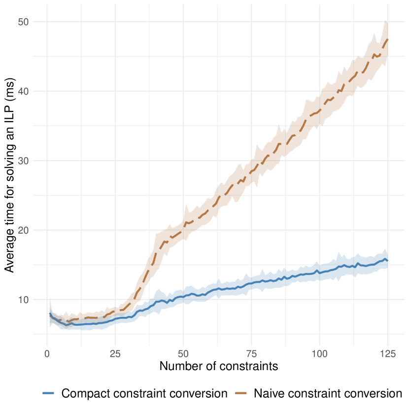
(b) Constraint density = $40\%$

Figure 1: Comparing encodings for conjunctive implications. The dashed brown lines show the average solver time (in milliseconds) across $100$ different runs for the naïve conversion to linear inequalities (§3), while the solid blue lines correspond to the compact conversion (§4). The shaded regions show one standard deviation. The two subfigures show different constraint densities, which control how many categorical variables are involved in the implications. Across both conditions, the compact encoding is more efficient.

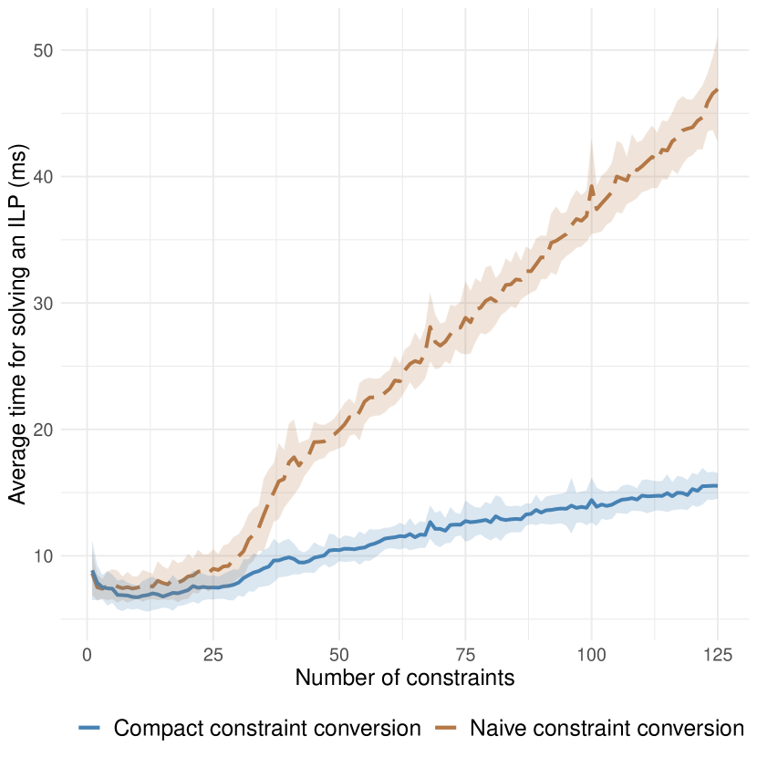
(a) Constraint density = $20\%$

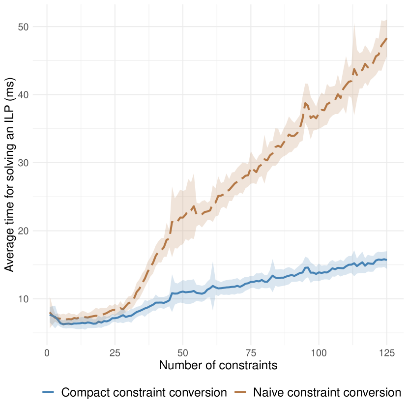
(b) Constraint density = $40\%$

Figure 2: Comparing encodings for disjunctive implications. See Figure 1 for details about the figure elements. As with conjunctions, compact encoding is more efficient.

5 Complex Building Blocks

So far we have seen basic building blocks that can help us declaratively construct output spaces for ILP inference. While any Boolean expression can be expressed as linear inequalities using only the tools introduced in §3, we saw in §4 that certain Boolean predicates (conditional forms) can be more compactly encoded as linear inequalities than the naïve expansion would suggest. In this section, we will look at more complex building blocks that abstract away larger predicates efficiently. We will use the fact that graph problems can be framed as linear programs to make these abstractions. We demonstrate two inference situations that frequently show up in NLP: spanning tree constraints and graph connectivity. We should note that other examples exist in the literature, for example, Germann et al. (2004) studied the use of ILPs to define the decoding problem for machine translation as a traveling salesman problem. We refer the reader to Trick (2005) for a discussion on using higher-order constructs for constrained inference.

Notation.

Since we will be dealing with constraints on graph structures, let us introduce the notation we will use for the rest of this section. We will denote vertices of a graph by integers $1,2,\ldots,n$ and edges by pairs $(i,j)$. Thus, for any vertex $i$, its outgoing edges are pairs of the form $(i,j)$ and incoming edges are pairs of the form $(j,i)$.

5.1 Spanning Trees

Our first example concerns spanning trees. Suppose each edge in the graph is associated with a score. Our goal is to identify the highest scoring collection of edges that form a spanning tree. Of course, efficient algorithms such as those of Borůvka, Prim or Kruskal solve the problem of finding maximum spanning trees for undirected graphs. If we are dealing with directed graphs, then the equivalent problem of finding the maximum spanning arborescence can be solved by the Chu-Liu-Edmonds’ algorithm. However, we might want to enforce additional task- or domain-specific constraints on the tree, rendering these efficient maximum spanning tree (or arborescence) methods unsuitable.

To simplify discourse, we will assume that we have a fully connected, undirected graph at hand. Our goal is to identify a subset of edges that form a tree over the vertices. The construction outlined in this section should be appropriately modified to suit variations.

Let us introduce a set of inference variables of the form $y_{{ij}}$ corresponding to an edge $(i,j)$ connecting vertices $i$ and $j$. Since we are considering an undirected graph, and will not allow self-edges in the spanning tree, we can assume that $i<j$ for all our inference variables. If the variable $y_{{ij}}$ is set to true, then the corresponding edge $(i,j)$ is selected in the final sub-graph. One method for enforcing a tree structure is to enumerate every possible cycle and add a constraint prohibiting it. However, doing so can lead to an exponential number of constraints, necessitating specialized solution strategies such as the cutting plane method (Riedel and Clarke, 2006).

Alternatively, we can exploit the connection between network flow problems and optimal trees to construct a more concise set of linear inequalities (Magnanti and Wolsey, 1995; Martins et al., 2009). In particular, we will use the well-studied relationship between the spanning tree problem and the single commodity flow problem. In the latter, we are given a directed graph, and we seek to maximize the total amount of a commodity (also called the flow) transported from a source node to one or more target nodes in the graph. Each edge in the graph has capacity constraints that limit how much flow it can carry.

Without loss of generality, suppose we choose vertex $1$ to be root of the tree. Then, we can write the requirement that the chosen vertices should form a tree using the single commodity flow model as follows:

1. Vertex 1 sends a flow of $n-1$ units to the rest of the graph.

2. Each other vertex consumes one unit of flow. The amount of flow consumed by the node is simply the difference between its incoming and outgoing flows.

3. Only edges that are chosen to be in the tree can carry flow.

To realize these three conditions, we will need to introduce auxiliary non-negative integer (or real) valued variables $\phi_{ij}$ and $\phi_{ji}$ that denote the flow associated with edge $(i,j)$ in either direction. Note that the flow variables are directed even though the underlying graph is undirected. These auxiliary variables do not feature in the ILP objective, or equivalently they are associated with zero costs in the objective.

Using these auxiliary variables, we get the following recipe:

Constraint 11: Select a spanning tree among vertices $1,2,\cdots,n$ of a undirected graph using edge variables $y_{{ij}}$, where $i<j$. Introduce new integer variables $\phi_{ij}$ and $\phi_{ji}$ for every such pair $i,j$.

$$\sum\limits_{j}\phi_{1j}-\sum\limits_{j}\phi_{j1}=n-1,$$

$$\mbox{for every vertex }i\in\{2,3,\cdots,n\}, \sum\limits_{j}\phi_{ji}-\sum\limits_{j}\phi_{ij}=1,$$

$$\mbox{for every edge }(i,j), \phi_{ij}\leq(n-1)y_{{ij}},$$

$$\mbox{for every edge }(i,j), \phi_{ji}\leq(n-1)y_{{ij}},$$

$$\mbox{for every edge }(i,j), \phi_{ij}\geq 0,$$

$$\mbox{for every edge }(i,j), \phi_{ji}\geq 0,$$

$$\sum\limits_{i,j}y_{{ij}}=n-1,$$

The first constraint here enforces that the chosen root sends a flow of $n-1$ units to the rest of the vertices. The second one says that every other vertex can consume exactly one unit of flow by mandating that the difference between the total incoming flow and the total outgoing flow for any vertex is 1. The third and fourth inequalities connect the inference variables $y_{{ij}}$ to the flow variables by ensuring that only edges that are selected (i.e. where $y_{{ij}}$ is true) can carry the flow. The next two constraints ensures that all the flows are non-negative. Finally, to ensure that the final sub-graph is a tree, the last constraint ensures that exactly $n-1$ edges are chosen. We will refer these constraints collectively as the Spanning Tree constraints over the variables $y_{{ij}}$.

There are other ways to efficiently formulate spanning tree constraints using linear inequalities. We refer the reader to Magnanti and Wolsey (1995) for an extensive discussion involving tree optimization problems and their connections to integer linear programming.

To illustrate the Spanning Tree construction, and how it can be used in conjunction with other constraints, let us look at an example.

Example 9.

Consider the graph in Figure 3(a). Suppose our goal is to find a tree that spans all the nodes in the graph, and has the highest cumulative weight. To this end, we can instantiate the recipe detailed above.

Each edge in the graph corresponds to one inference variable that determines whether the corresponding node is in the tree or not. The variables are weighted in the objective as per the edge weight. (We do not need to add variables for any edge not shown in the figure; they are weighted $-\infty$, and will never get selected.) Collectively, all the edge variables, scaled by their corresponding weights, gives us the ILP objective to maximize, namely:

$$10y_{{12}}+50y_{{13}}+5y_{{15}}+11y_{{23}}+15y_{{15}}-9y_{{34}}-7y_{{35}}-50y_{{45}}$$

Next, we can instantiate the spanning tree constraints using flow variables $\{\phi_{12},\phi_{21},\cdots\}$. To avoid repetition, we will not rewrite the constraints here. Solving the (mixed) integer linear program with the flow constraints gives us an assignment to the $y_{{ij}}$ variables that corresponds to the tree in Figure 3(b). Of course, if our goal was merely to find the maximum spanning tree in the graph, we need not (and perhaps, should not) seek to do so via an ILP, and instead use one of the named greedy algorithms mentioned earlier that is specialized for this purpose.

Now, suppose we wanted to find the second highest scoring tree. Such a situation may arise, for example, to find the top-$k$ solutions of an inference problem. To do so, we can add a single extra constraint in addition to the flow constraints that prohibit the tree from Figure 3 (b). In other words, the solution we seek should satisfy the following constraint:

$$\neg\left(y_{{13}}\land y_{{23}}\land y_{{25}}\land y_{{34}}\right)$$

We can convert this constraint into linear inequalities using the recipies we have seen previously in this survey. Adding the inequality into the ILP from above will give us the tree in Figure 3(c).

Figure 3: An undirected graph to illustrate the spanning tree constraints. The goal is to find the two highest scoring trees spanning the nodes in subfigure (a). Example 9 shows how to generate the two trees in subfigures (b) and (c) incrementally. The directed edges in the tree show the direction of commodity flow in the solutions to the mixed integer programs.

5.2 Graph Connectivity

Our second complex building block involves distilling a connected sub-graph from a given graph. Suppose our graph at hand is directed and we seek to select a sub-graph that spans all the nodes and is connected. We can reduce this to the spanning tree constraint by observing that any connected graph should contain a spanning tree. This observation gives us the following solution strategy: Construct an auxiliary problem (i.e, finding a spanning tree) whose solution will ensure the connectivity constraints we need.

Let inference variables $y_{{ij}}$ denote the decision that the edge $(i,j)$ is selected. To enforce the connectivity constraints, we will introduce auxiliary Boolean inference variables $z_{ij}$ (with zero objective coefficients) for every edge $(i,j)$ or $(j,i)$ that is in the original graph. In other words, the auxiliary variables we introduce are undirected.

Using these auxiliary variables, we can state the connectivity requirement as follows:

1. The inference variables $z_{ij}$ form a spanning tree over the nodes.

2. If $z_{ij}$ is true, then either the edge $(i,j)$ or the edge $(j,i)$ should get selected.

We can write these two requirements using the building blocks we have already seen.

Constraint 12: Find a connected spanning sub-graph of the nodes $1,2,\cdots,n$

$$\mbox{{\sc Spanning Tree} constraints over variables }z_{ij},$$

$$\mbox{for every }(i,j)\mbox{ such that }i<j,\quad\quad z_{ij}\rightarrow y_{{ij}}\vee y_{{ji}}.$$

Each of these constraints can be reduced to a collection of linear inequalities using the tools we have seen so far. We will see an example of how a variant of this recipe can be used in §6.2. In the construction above, the $z$’s help set up the auxiliary spanning tree problem. Their optimal values are typically disregarded, and it is the assignment to the $y$’s that constitute the solution to the original problem.

5.3 Other Graph Problems

In general, if the problem at hand can be written as a known and tractable graph problem, then there are various efficient ways to instantiate linear inequalities that encode the structure of the output graph. We refer the reader to resources such as Papadimitriou and Steiglitz (1982), Magnanti and Wolsey (1995) and Schrijver (1998) for further reference. We also refer the reader to the AD³ algorithm (Martins et al., 2015) that supports the coarse decomposition of inference problems to take advantage of graph algorithms directly.

5.4 Soft Constraints

The constraints discussed so far in this survey are hard constraints. That is, they prohibit certain assignments of the decision variables. In contrast, a soft constraint merely penalizes assignments that violates them rather than disallowing them. Soft constraints can be integrated into the integer linear programming framework in a methodical fashion. Srikumar (2013) explains the process of adding soft constraints into ILP inference. Here we will see a brief summary.

As before, suppose we have an inference problem expressed as an integer linear program:

$$\max_{{{\bf y}}} \sum\limits_{i}c_{{i}}y_{{i}}$$

s.t. $${{\bf y}}\in\mathcal{Y},$$

$$y_{{i}}\in\{0,1\}.$$

Here, the requirement that ${{\bf y}}\in\mathcal{Y}$ is assumed to be stated as linear inequalities. However, as we have seen in the previous sections, they could be equivalently stated as Boolean expressions.

If, in addition to the existing constraint, we have an additional Boolean constraint $C({\bf y})$ written in terms of inference variables ${\bf y}$. Instead of treating this as a hard constraint, we only wish to penalize assignments ${\bf y}$ that violate this constraint by a penalty term $\rho_{C}$. We will consider the case where $\rho_{C}$ is independent of ${\bf y}$. To address inference in such a scenario, we can introduce a new Boolean variable $z$ that tracks whether the constraint is not satisfied. That is,

$$z\leftrightarrow\neg C({\bf y}).$$ (8)

If the constraint is not satisfied, then the corresponding assignment to the decision variables should be penalized by $\rho_{C}$. We can do so by adding a term $-z\rho_{C}$ to the objective of the original ILP. Since the constraint (8) that defines the new variable $z$ is also a Boolean expression, it can be converted into a set of linear inequalities.

This procedure gives us the following new ILP that incorporates the soft constraint:

$$\max_{{{\bf y}},z} \sum\limits_{i}c_{{i}}y_{{i}}-z\rho_{C}$$

s.t. $${{\bf y}}\in\mathcal{Y},$$

$$z\leftrightarrow\neg C({\bf y}),$$

$$y_{{i}},z\in\{0,1\}.$$

We can summarize the recipe for converting soft constraints into larger ILPs below:

Constraint 13: Soft constraint $C({\bf y})$ with a penalty $\rho_{C}$

Add a Boolean variable $$z -\rho_{C}$$ to the objective with coefficient

$$\mbox{Add constraint }z\leftrightarrow\neg C({\bf y})$$

6 Worked Examples

In this section, we will work through two example NLP tasks that use the framework that we have seen thus far. First, we will look at the problem of predicting sequences, where efficient inference algorithms exist. Then, we will see the task of predicting relationships between events in text, where we need the full ILP framework even for a simple setting.

6.1 Sequence Labeling

Our first example is the problem of sequence labeling. Using the tools we have seen so far, we will write down prediction in a first order sequence model as an integer linear program.

Example 10 (Sequence Labeling).

Suppose we have a collection of $n$ categorical decisions, each of which can take one of three values $\mathcal{L}=\{{\tt a},{\tt b},{\tt c}\}$. We can think of these $n$ decisions as slots that are waiting to be assigned one the three labels. Each slot has an intrinsic preference for one of the three labels. Additionally, the label at each slot is influenced by the label of the previous slot. The goal of inference is to find a sequence of labels that best accommodates both the intrinsic preferences of each slot and the influence of the neighbors.

Let us formalize this problem. There are two kinds of scoring functions. The decision at the $i^{th}$ slot is filled with a label ${\tt L}$ is associated with an emission score $c_{{i:{\tt L}}}$ that indicates the intrinsic preference of the slot getting the label. Additionally, pairs of decisions in the sequence are scored using transition scores. That is, the outcome that the $i^{th}$ label is ${\tt L_{1}}$ and the $j^{th}$ label is ${\tt L_{2}}$ is jointly scored using $c_{{{\tt L_{1}},{\tt L_{2}}}}$. (Notice that the transition score is independent of $i$ in this formulation.) Now, our goal is find a label assignment to all $n$ slots that achieves the maximum total score.

Figure 4: An example factor graph for a sequence model. This figure illustrates the case of five decisions in a sequence. Circles denote random variables whose assignment we seek and the squares represent factors or scoring functions as described in the text.

Figure 4 gives the usual pictorial representation of this predictive problem. A first-order sequence labeling problem of this form is ubiquitous across NLP for tasks such as part-of-speech tagging, text chunking and various information extraction problems. There are different ways to frame this problem as an ILP. We will employ one that best illustrates the use of the techniques we have developed so far.

First, let us start with the decision variables. There are two kinds of decisions—emissions and transitions—that contribute to the total score. Let $y_{{i:{\tt L}}}$, scored by $c_{{i:{\tt L}}}$, denote the decision that the $i^{th}$ label is ${\tt L}$. Let $y_{{i:{\tt L_{1}},{\tt L_{2}}}}$ denote the decision that the $i^{th}$ label is ${\tt L_{1}}$ and the next one is ${\tt L_{2}}$. This transition is scored by $c_{{{\tt L_{1}},{\tt L_{2}}}}$. These variables and their associated scores give us the following objective function for the inference:

$$\max_{{{\bf y}}}\sum\limits_{i=1}^{n}\sum\limits_{{\tt L}\in\mathcal{L}}c_{{i:{\tt L}}}\cdot y_{{i:{\tt L}}}+\sum\limits_{i=1}^{n-1}\sum\limits_{{\tt L_{1}},{\tt L_{2}}\in\mathcal{L}}c_{{{\tt L_{1}},{\tt L_{2}}}}\cdot y_{{i:{\tt L_{1}},{\tt L_{2}}}}.$$ (9)

Note that the objective simply accumulates scores from every possible decision that can be made during inference. For the sake of simplicity, we are ignoring initial states in this discussion, but they can be easily folded into the objective.

Now that the inference variables are defined, we need to constrain them. We have two kinds of constraints:

1. Each slot can take exactly one label in $\mathcal{L}=\{{\tt a},{\tt b},{\tt c}\}$. Once again, we instantiate the Multiclass Classification as an ILP construction (§3.2) to get

   $$\forall i\in\{1,2,\cdots,n\};\sum\limits_{L\in\mathcal{L}}y_{{i:{\tt L}}}=1.$$ (10)

   These equations give us $n$ linear constraints in all.

2. The transition decisions and the emission decisions should agree with each other. Written down in logic, this condition can be stated as:

   $$\forall~{}i\in\{1,2,\cdots,n\};\quad\forall~{}{\tt L_{1}},{\tt L_{2}}\in\mathcal{L};\quad y_{{i:{\tt L_{1}},{\tt L_{2}}}}\leftrightarrow y_{{i:{\tt L_{1}}}}\wedge y_{{i+1:{\tt L_{2}}}}$$

   Together, these $n|\mathcal{L}|^{2}$ constraints ensure that the output is a valid sequence. Since each of them is a conjunctive biconditional form (§4.2), we get the following linear inequalities representing the constraints:

   $$\forall i,{\tt L_{1}},{\tt L_{2}}; -2y_{{i:{\tt L_{1}},{\tt L_{2}}}}+y_{{i:{\tt L_{1}}}}+y_{{i+1:{\tt L_{2}}}}\geq 0$$ (11)

   $$y_{{i:{\tt L_{1}},{\tt L_{2}}}}-y_{{i:{\tt L_{1}}}}-y_{{i+1:{\tt L_{2}}}}\geq-1$$ (12)

   In all, we get $2n|\mathcal{L}|^{2}$ linear inequalities to represent these consistency constraints.

The objective (9) and the constraints (10), (11) and (12) together form the integer linear program for sequence labeling.

It is important to note once again that here, we are only using the integer linear programs as a declarative language to state inference problems, not necessarily for solving them. Specifically for the sequence labeling problem framed as a first-order Markov model, the Viterbi algorithm offers a computationally efficient solution to the inference problem. However, we may wish to enforce constraints that renders the Viterbi algorithm unusable.

The strength of the ILP formulation comes from the flexibility it gives us. For example, consider the well-studied problem of part-of-speech tagging. Suppose, we wanted to only consider sequences where there is at least one ${\tt verb}$ in the final output. It is easy to state this using the following constraint:

$$\sum\limits_{i=1}^{n}y_{{i:{\tt verb}}}\geq 1.$$ (13)

With this constraint, we can no longer use the vanilla Viterbi algorithm for inference. But, by separating the declaration of the problem from the computational strategies for solving them, we can at least write down the problem formally, perhaps allowing us to use a different algorithm, say Lagrangian relaxation (Everett III, 1963; Lemaréchal, 2001), or a call to a black box ILP solver for solving the new inference problem.

6.2 Recognizing Event-Event Relations

Our second example involves identifying relationships between events in text. While the example below is not grounded directly in any specific instantiation of the task, it represents a simplified version of the inference problem addressed by Berant et al. (2014); Ning et al. (2018a, b); Wang et al. (2020).

Example 11 (Event-Event Relations).

Suppose we have a collection of events denoted by $E=\{e_{1},e_{2},\cdots,e_{n}\}$ that are attested in some text. Our goal is to identify causal relationships between these events. That is, for any pair of events $e_{i}$ and $e_{j}$, we seek a directed edge that can be labeled with one of a set of labels $R=$ {Cause, Prevent, None} respectively indicating that the event $e_{i}$ causes, prevents or is unrelated to event $e_{j}$.

For every pair of events $e_{i}$ and $e_{j}$, we will introduce decision variables $y_{{ij:r}}$ for each relation $r\in R$ denoting that the edge $(i,j)$ is labeled with the relation $r$. Each decision may be assigned a score $c_{{ij:r}}$ by a learned scoring function. Thus, the goal of inference is to find a score maximizing set of assignments to these variables. This gives us the following objective:

$$\sum\limits_{e_{i},e_{j}\in E}\sum\limits_{r\in R}c_{{ij:r}}\cdot y_{{ij:r}}.$$ (14)

Suppose we have three sets of constraints that restrict the set of possible assignments to the inference variables. These constraints are a subset of the constraints used to describe biological processes by Berant et al. (2014).

1. Each edge should be assigned exactly one label in $R$. This is the Multiclass Classification as an ILP construction, giving us

   $$\forall e_{i},e_{j}\in E,\sum\limits_{r\in R}y_{{ij:r}}=1.$$ (15)

2. If an event $e_{i}$ causes or prevents $e_{j}$, then $e_{j}$ can neither cause nor prevent $e_{i}$. In other words, if a Cause or a Prevent relation is selected for the $(i,j)$ edge, then the None relation should be chosen for the $(j,i)$ edge. We can write this as a logical expression as:

   $$\forall e_{i},e_{j}\in E,y_{{ij:\mbox{\footnotesize\sc Cause}}}\vee y_{{ij:\mbox{\footnotesize\sc Prevent}}}\rightarrow y_{{ji:{\mbox{\footnotesize\sc None}}}}.$$

   This is an example of a disjunctive implication (§4.2), which we can write using linear inequalities as:

   $$\forall e_{i},e_{j}\in E,-y_{{ij:\mbox{\footnotesize\sc Cause}}}-y_{{ij:\mbox{\footnotesize\sc Prevent}}}+2y_{{ji:\mbox{\footnotesize\sc None}}}\geq 0.$$ (16)

3. The events should form a connected component using the non-None edges. This constraint invokes the graph connectivity construction from §5.2. To instantiate the construction, let us introduce auxiliary Boolean variables $z_{ij}$ that indicates that the events $e_{i}$ and $e_{j}$ are connected with an edge that is not labeled None in at least one direction, i.e., the edge from $e_{i}$ to $e_{j}$ or the one in the other direction has a non-Nonelabel. As before, let $\phi_{ij}$ denote the non-negative real valued flow variables along a directed edge $(i,j)$. Following §5.2, we will require that the $z_{ij}$’s form a spanning tree.

   First, the auxiliary variables $z_{ij}$ should correspond to events $e_{i}$ and $e_{j}$ that are connected by a non-None edge in either direction. That is,

   $$\forall e_{i},e_{j}\in E~{}\text{where}~{}i<j,~{} z_{ij}\rightarrow\left(\exists~{}r\neq\mbox{\footnotesize\sc None},~{}\text{s.t.}~{}y_{{ij:r}}\vee y_{{ji:r}}\right),$$ (17)

   The existential form on the right hand side of the implication can be written as a disjunction, thus giving us a disjunctive implication. For brevity, we will not expand these Boolean expressions into linear inequalities.

   Second, an arbitrarily chosen event $e_{1}$ sends out $n-1$ units of flow, and each event consumes one one unit of flow.

   $$\sum_{j}\phi_{1j}-\sum_{j}\phi_{j1}=n-1,$$ (18)

   $$\forall e_{i}\in E, \sum_{j}\phi_{ij}-\sum_{j}\phi_{ji}=1.$$ (19)

   Third, the commodity flow should only happen along the edges that are selected by the auxiliary variables.

   $$\forall e_{i},e_{j}\in E~{}\text{where}~{}i<j,~{}\phi_{ij}\leq(n-1)z_{ij}$$ (20)

   Finally, the auxiliary variables should form a tree. That is, exactly $n-1$ of them should be selected.

   $$\sum\limits_{i,j}z_{ij}=n-1.$$ (21)

We can write the final inference problem as the problem of maximizing the objective (14) with respect to the inference variables ${{\bf y}}$, the auxiliary variables $z_{ij}$ and the flow variables $\phi_{ij}$ subject to the constraints listed in Equations 15 to 21. Of course, the decision variables ${{\bf y}}$ and the auxiliary variables $z_{ij}$ are $0$-$1$ variables, while the flow variables are non-negative real valued ones.

7 Final Words

We have seen a collection of recipes that can help to encode inference problems as instances of integer linear programs. Each recipe focuses on converting a specific kind of predicate into one or more linear inequalities that constitute the constraints for the discrete optimization problem. The conversion of predicates to linear inequalities is deterministic and, in fact, can be seen as a compilation step, where the user merely specifies constraints in first-order logic and an inference compiler produces efficient ILP formulations. Some programs that allow declarative specification of inference include Learning Based Java (Rizzolo, 2012), Saul Kordjamshidi et al. (2016) and DRaiL Pacheco and Goldwasser (2021).

It should be clear from this tutorial-style survey that there may be multiple ways to encode the same inference problem as integer programs. The best encoding may depend on how the integer program is solved. Current solvers (circa 2022) seem to favor integer programs with fewer constraints that are dense in terms of the number of variables each one involves. To this end, we saw two strategies: We either collapsed multiple logical constraints that lead to sparse inequalities to fewer dense ones, or formulated the problem in terms of known graph problems.

While it is easy to write down inference problems, it is important to keep the computational properties of the inference problem in mind. The simplicity of design can make it easy to end up with large and intractable inference problems. For example, for the event relations example from §6.2, if we had tried to identify both the events and their relations using a single integer program (by additionally specifying event decision variables), the approach suggested here can lead to ILP instances that are difficult to solve with current solvers.

A survey on using integer programming for modeling inference would be remiss without mentioning techniques for solving the integer programs. The easiest approach is to use an off-the-shelf solver. Currently, the fastest ILP solver is the Gurobi solver; other solvers include the CPLEX Optimizer, the FICO Xpress-Optimizer, lp_solve, and GLPK. The advantage of using off-the-shelf solvers is that we can focus on the problem at hand. However, using such solvers prevents us from using task-driven specialized strategies for inference, if they exist. Sometimes, even though we can write the inference problem as an ILP, we may be able to design an efficient algorithm for solving it by taking advantage of the structure of the problem. Alternatively, we can relax the problem by simply dropping the $\{0,1\}$ constraints over the inference variables and instead restricting them to be real valued in the range $[0,1]$. We could also employ more sophisticated relaxation methods such as Lagrangian relaxation (Everett III, 1963; Lemaréchal, 2001; Geoffrion, 2010; Chang and Collins, 2011), dual decomposition (Rush and Collins, 2012; Rush et al., 2010; Koo et al., 2010), or the augmented Lagrangian method (Martins et al., 2011a, b; Meshi and Globerson, 2011; Martins et al., 2015).

The ability to write down prediction problems in a declarative fashion (using predicate logic or equivalently as ILPs) has several advantages. First, we can focus on the definition of the task we want to solve rather than the algorithmic details of how to solve it. Second, because we have a unifying language for reasoning about disparate kinds of tasks, we can start reasoning about properties of inference in a task-independent fashion. For example, using such an abstraction, we can amortize inference costs over the lifetime of the predictor (Srikumar et al., 2012; Kundu et al., 2013; Chang et al., 2015; Pan and Srikumar, 2018).

Finally, recent successes in NLP have used neural models with pre-trained representations such as BERT (Devlin et al., 2019), RoBERTa (Liu et al., 2019) and others. The unification of such neural networks and declarative modeling with logical constraints is an active area of research today (Xu et al., 2018; Li and Srikumar, 2019; Li et al., 2019; Fischer et al., 2019; Nandwani et al., 2019; Li et al., 2020; Wang et al., 2020; Asai and Hajishirzi, 2020; Giunchiglia and Lukasiewicz, 2021; Grespan et al., 2021; Pacheco and Goldwasser, 2021; Ahmed et al., 2022, inter alia). This area is intimately connected with the area of neuro-symbolic modeling which seeks to connect neural models with symbolic reasoning. We refer the reader to Garcez and Lamb (2020); Kautz (2022); Pacheco et al. (2022) for recent perspectives on the topic. The declarative modeling strategy supported by the kind of inference outlined in this tutorial may drive the integration of complex symbolic reasoning with expressive neural models, which poses difficulties for current state-of-the-art models.

References

- Ahmed et al. (2022) Kareem Ahmed, Tao Li, Thy Ton, Quan Guo, Kai-Wei Chang, Parisa Kordjamshidi, Vivek Srikumar, Guy Van den Broeck, and Sameer Singh. PYLON: A PyTorch framework for learning with constraints. In NeurIPS 2021 Competitions and Demonstrations Track, pages 319–324. PMLR, 2022.
- Asai and Hajishirzi (2020) Akari Asai and Hannaneh Hajishirzi. Logic-Guided Data Augmentation and Regularization for Consistent Question Answering. In Proceedings of the 58th Annual Meeting of the Association for Computational Linguistics, 2020.
- Berant et al. (2014) Jonathan Berant, Vivek Srikumar, Pei-Chun Chen, Abby Vander Linden, Brittany Harding, Brad Huang Peter Clark, and Christopher D. Manning. Modeling Biological Processes for Reading Comprehension. In Proceedings of the 2014 Conference on Empirical Methods in Natural Language Processing (EMNLP), pages 1499–1510, 2014.
- Brachman and Levesque (1985) Ronald J. Brachman and Hector J. Levesque. Readings in Knowledge Representation. Morgan Kaufmann Publishers Inc., San Francisco, CA, USA, 1985. ISBN 978-0-934613-01-9.
- Chandra and Harel (1985) Ashok K Chandra and David Harel. Horn clause queries and generalizations. The Journal of Logic Programming, 2(1):pp. 1–15, 1985.
- Chang et al. (2015) Kai-Wei Chang, Shyam Upadhyay, Gourab Kundu, and Dan Roth. Structural learning with amortized inference. In Proceedings of the Twenty-Ninth AAAI Conference on Artificial Intelligence, pages 2525—2531, January 2015.
- Chang et al. (2010) Ming-Wei Chang, Dan Goldwasser, Dan Roth, and Vivek Srikumar. Discriminative Learning over Constrained Latent Representations. In Human Language Technologies: The 2010 Annual Conference of the North American Chapter of the Association for Computational Linguistics, pages 429—437, 2010.
- Chang and Collins (2011) Yin-Wen Chang and Michael Collins. Exact Decoding of Phrase-Based Translation Models through Lagrangian Relaxation. In Proceedings of the 2011 Conference on Empirical Methods in Natural Language Processing, pages 26—37, July 2011.
- Choi et al. (2006) Yejin Choi, Eric Breck, and Claire Cardie. Joint Extraction of Entities and Relations for Opinion Recognition. In Proceedings of the 2006 Conference on Empirical Methods in Natural Language Processing, pages 431–439, 2006.
- Clarke and Lapata (2008) James Clarke and Mirella Lapata. Global Inference for Sentence Compression: An Integer Linear Programming Approach. Journal of Artificial Intelligence Research, 31:399—429, 2008.
- Denis and Baldridge (2009) Pascal Denis and Jason Baldridge. Global joint models for coreference resolution and named entity classification. Procesamiento del Lenguaje Natural, 42:87–96, 2009.
- Denis and Muller (2011) Pascal Denis and Philippe Muller. Predicting globally-coherent temporal structures from texts via endpoint inference and graph decomposition. In Proceedings of the Twenty-Second International Joint Conference on Artificial Intelligence, pages 1788—1793, 2011.
- Devlin et al. (2019) Jacob Devlin, Ming-Wei Chang, Kenton Lee, and Kristina Toutanova. BERT: Pre-training of Deep Bidirectional Transformers for Language Understanding. In Proceedings of the 2019 Conference of the North American Chapter of the Association for Computational Linguistics: Human Language Technologies, Volume 1 (Long and Short Papers), 2019.
- Everett III (1963) Hugh Everett III. Generalized Lagrange Multiplier Method for Solving Problems of Optimum Allocation of Resources. Operations Research, 11(3):pp. 399–417, 1963.
- Fischer et al. (2019) Marc Fischer, Mislav Balunovic, Dana Drachsler-Cohen, Timon Gehr, Ce Zhang, and Martin Vechev. DL2: Training and Querying Neural Networks with Logic. In International Conference on Machine Learning, 2019.
- Garcez and Lamb (2020) Artur d’Avila Garcez and Luis C Lamb. Neurosymbolic AI: the 3rd wave. arXiv preprint arXiv:2012.05876, 2020.
- Geoffrion (2010) Arthur M Geoffrion. Lagrangian relaxation for integer programming. In 50 Years of Integer Programming 1958-2008, pages 243–281. Springer, 2010.
- Germann et al. (2004) Ulrich Germann, Michael Jahr, Kevin Knight, Daniel Marcu, and Kenji Yamada. Fast and optimal decoding for machine translation. Artificial Intelligence, 154:127–143, April 2004.
- Giunchiglia and Lukasiewicz (2021) Eleonora Giunchiglia and Thomas Lukasiewicz. Multi-Label Classification Neural Networks with Hard Logical Constraints. Journal of Artificial Intelligence Research, 72:759–818, November 2021. ISSN 1076-9757. doi: 10.1613/jair.1.12850.
- Goldwasser and Roth (2008) Dan Goldwasser and Dan Roth. Transliteration as Constrained Optimization. In Proceedings of the 2008 Conference on Empirical Methods in Natural Language Processing, pages 353–362, 2008.
- Goldwasser and Zhang (2016) Dan Goldwasser and Xiao Zhang. Understanding Satirical Articles Using Common-Sense. Transactions of the Association for Computational Linguistics, 4:537–549, 2016.
- Grespan et al. (2021) Mattia Medina Grespan, Ashim Gupta, and Vivek Srikumar. Evaluating Relaxations of Logic for Neural Networks: A Comprehensive Study. In Twenty-Ninth International Joint Conference on Artificial Intelligence, volume 3, pages 2812–2818, 2021. doi: 10.24963/ijcai.2021/387.
- Guéret et al. (2002) Christelle Guéret, Christian Prins, Marc Sevaux, and Susanne Heipcke. Applications of optimization with Xpress-MP. Dash Optimization Blisworth, UK, 2002.
- Iverson (1962) Kenneth E Iverson. A Programming Language. John Wiley & Sons, Inc., 1962.
- Karp (1972) Richard M Karp. Reducibility among combinatorial problems. In Complexity of Computer Computations, pages 85–103. Springer, 1972.
- Kautz (2022) Henry Kautz. The third AI summer: AAAI Robert S. Engelmore memorial lecture. AI Magazine, 43(1):105–125, 2022.
- Khardon and Roth (1996) Roni Khardon and Dan Roth. Reasoning with Models. Artificial Intelligence, 87(1-2):187–213, 1996.
- Knuth (1992) Donald E Knuth. Two notes on notation. The American Mathematical Monthly, 99(5):403–422, 1992.
- Koo et al. (2010) Terry Koo, Alexander M. Rush, Michael Collins, Tommi Jaakkola, and David Sontag. Dual Decomposition for Parsing with Non-Projective Head Automata. In Proceedings of the 2010 Conference on Empirical Methods in Natural Language Processing, pages 1288—1298, 2010.
- Kordjamshidi et al. (2016) Parisa Kordjamshidi, Daniel Khashabi, Christos Christodoulopoulos, Bhargav Mangipudi, Sameer Singh, and Dan Roth. Better call Saul: Flexible programming for learning and inference in NLP. In Proceedings of COLING 2016, the 26th International Conference on Computational Linguistics: Technical Papers, pages 3030–3040, Osaka, Japan, December 2016. The COLING 2016 Organizing Committee. URL https://aclanthology.org/C16-1285.
- Kundu et al. (2013) Gourab Kundu, Vivek Srikumar, and Dan Roth. Margin-based Decomposed Amortized Inference. In Proceedings of the 51st Annual Meeting of the Association for Computational Linguistics (Volume 1: Long Papers), pages 905–913, 2013.
- Lemaréchal (2001) Claude Lemaréchal. Lagrangian Relaxation. In Computational Combinatorial Optimization, pages 112–156, 2001.
- Li and Srikumar (2016) Tao Li and Vivek Srikumar. Exploiting Sentence Similarities for Better Alignments. In Proceedings of the 2016 Conference on Empirical Methods in Natural Language Processing, pages 2193–2203, 2016.
- Li and Srikumar (2019) Tao Li and Vivek Srikumar. Augmenting Neural Networks with First-order Logic. In Proceedings of the 57th Annual Meeting of the Association for Computational Linguistics, 2019.
- Li et al. (2019) Tao Li, Vivek Gupta, Maitrey Mehta, and Vivek Srikumar. A Logic-Driven Framework for Consistency of Neural Models. In Proceedings of the 2019 Conference on Empirical Methods in Natural Language Processing and the 9th International Joint Conference on Natural Language Processing (EMNLP-IJCNLP), 2019.
- Li et al. (2020) Tao Li, Parth Anand Jawale, Martha Palmer, and Vivek Srikumar. Structured Tuning for Semantic Role Labeling. In Proceedings of the 58th Annual Meeting of the Association for Computational Linguistics, 2020.
- Liu et al. (2019) Yinhan Liu, Myle Ott, Naman Goyal, Jingfei Du, Mandar Joshi, Danqi Chen, Omer Levy, Mike Lewis, Luke Zettlemoyer, and Veselin Stoyanov. RoBERTa: A Robustly Optimized BERT Pretraining Approach. arXiv preprint arXiv:1907.11692, 2019.
- Magnanti and Wolsey (1995) Thomas L Magnanti and Laurence A Wolsey. Optimal Trees. Handbooks in operations research and management science, 7:503–615, 1995.
- Martins et al. (2009) André Martins, Noah A. Smith, and Eric Xing. Concise Integer Linear Programming Formulations for Dependency Parsing. In Proceedings of the Joint Conference of the 47th Annual Meeting of the ACL and the 4th International Joint Conference on Natural Language Processing of the AFNLP, pages 342—350, 2009.
- Martins et al. (2011a) André Martins, Mario Figueiredor, Pedro Aguiar, Noah A. Smith, and Eric Xing. An Augmented Lagrangian Approach to Constrained MAP Inference. In Proceedings of the 28th International Conference on International Conference on Machine Learning, pages 169–176, 2011a.
- Martins et al. (2011b) André F. T. Martins, Noah A. Smith, Mário Figueiredo, and Pedro Aguiar. Dual decomposition with many overlapping components. In Proceedings of the Conference on Empirical Methods in Natural Language Processing, pages 238–249, 2011b.
- Martins et al. (2015) André F. T. Martins, Mário A. T. Figueiredo, Pedro M. Q. Aguiar, Noah A. Smith, and Eric P. Xing. AD3: Alternating Directions Dual Decomposition for MAP Inference in Graphical Models. The Journal of Machine Learning Research, 16(1):495–545, January 2015.
- Meshi and Globerson (2011) Ofer Meshi and Amir Globerson. An Alternating Direction Method for Dual MAP LP Relaxation. In Dimitrios Gunopulos, Thomas Hofmann, Donato Malerba, and Michalis Vazirgiannis, editors, Machine Learning and Knowledge Discovery in Databases, Lecture Notes in Computer Science, pages 470–483, 2011.
- Nandwani et al. (2019) Yatin Nandwani, Abhishek Pathak, and Parag Singla. A Primal Dual Formulation For Deep Learning With Constraints. In Advances in Neural Information Processing Systems, pages 12157–12168, 2019.
- Ning et al. (2018a) Qiang Ning, Zhili Feng, Hao Wu, and Dan Roth. Joint Reasoning for Temporal and Causal Relations. In Proc. of the Annual Meeting of the Association for Computational Linguistics (ACL), pages 2278–2288, Melbourne, Australia, 7 2018a. Association for Computational Linguistics. URL http://cogcomp.org/papers/NingFeWuRo18.pdf.
- Ning et al. (2018b) Qiang Ning, Hao Wu, Haoruo Peng, and Dan Roth. Improving Temporal Relation Extraction with a Globally Acquired Statistical Resource. In Proc. of the Annual Conference of the North American Chapter of the Association for Computational Linguistics (NAACL), pages 841–851, New Orleans, Louisiana, 6 2018b. Association for Computational Linguistics. URL http://cogcomp.org/papers/NingWuPeRo18.pdf.
- Noessner et al. (2013) Jan Noessner, Mathias Niepert, and Heiner Stuckenschmidt. RockIt: Exploiting Parallelism and Symmetry for MAP Inference in Statistical Relational Models. In Proceedings of the Twenty-Seventh AAAI Conference on Artificial Intelligence, 2013.
- Pacheco and Goldwasser (2021) Maria Leonor Pacheco and Dan Goldwasser. Modeling Content and Context with Deep Relational Learning. Transactions of the Association for Computational Linguistics, 9, February 2021.
- Pacheco et al. (2022) Maria Leonor Pacheco, Sean Welleck, Yejin Choi, Vivek Srikumar, Dan Goldwasser, and Dan Roth. NS4NLP: Neuro-Symbolic Modeling for NLP. In COLING (Tutorials), 2022. URL https://ns4nlp-coling.github.io/.
- Pan and Srikumar (2018) Xingyuan Pan and Vivek Srikumar. Learning to Speed Up Structured Output Prediction. In Proceedings of the 35th International Conference on Machine Learning, pages 3996–4005, 2018.
- Papadimitriou and Steiglitz (1982) Christos Papadimitriou and Kenneth Steiglitz. Combinatorial Optimization: Algorithms and Complexity. Courier Corporation, 1982.
- Punyakanok et al. (2008) Vasin Punyakanok, Dan Roth, and Wen-tau Yih. The Importance of Syntactic Parsing and Inference in Semantic Role Labeling. Computational Linguistics, 34(2):257–287, 2008.
- Ravi et al. (2010) Sujith Ravi, Jason Baldridge, and Kevin Knight. Minimized Models and Grammar-Informed Initialization for Supertagging with Highly Ambiguous Lexicons. In Proceedings of the 48th Annual Meeting of the Association for Computational Linguistics, pages 495–503, 2010.
- Riedel and Clarke (2006) Sebastian Riedel and James Clarke. Incremental Integer Linear Programming for Non-Projective Dependency Parsing. In Proceedings of the 2006 Conference on Empirical Methods in Natural Language Processing, pages 129–137, 2006.
- Rizzolo (2012) Nicholas Rizzolo. Learning based programming. PhD thesis, University of Illinois at Urbana-Champaign, 2012.
- Rizzolo and Roth (2007) Nicholas Rizzolo and Dan Roth. Modeling Discriminative Global Inference. In Proceedings of the First International Conference on Semantic Computing (ICSC), pages 597–604, Irvine, California, September 2007. IEEE.
- Roth (1996) Dan Roth. Learning in Order to Reason: The Approach. In Proceedings of the Conference on Current Trends in Theory and Practice of Informatics (SOFSEM), pages 113–124, 1996.
- Roth and Yih (2004) Dan Roth and Wen-tau Yih. A Linear Programming Formulation for Global Inference in Natural Language Tasks. In Proceedings of the Eighth Conference on Computational Natural Language Learning (CoNLL-2004) at HLT-NAACL 2004, pages 1—8, 2004.
- Roth and Yih (2005) Dan Roth and Wen-tau Yih. Integer linear programming inference for conditional random fields. In Proceedings of the 22nd International Conference on Machine Learning, pages 736–743, 2005.
- Roth and Yih (2007) Dan Roth and Wen-tau Yih. Global Inference for Entity and Relation Identification via a Linear Programming Formulation. In Lise Getoor and Ben Taskar, editors, Introduction to Statistical Relational Learning, pages 553–580. MIT Press, 2007.
- Roy and Roth (2015) Subhro Roy and Dan Roth. Solving General Arithmetic Word Problems. In Proceedings of the 2015 Conference on Empirical Methods in Natural Language Processing, pages 1743–1752, September 2015.
- Rush and Collins (2012) Alexander M Rush and MJ Collins. A Tutorial on Dual Decomposition and Lagrangian Relaxation for Inference in Natural Language Processing. Journal of Artificial Intelligence Research, 45:305–362, 2012.
- Rush et al. (2010) Alexander M. Rush, David Sontag, Michael Collins, and Tommi Jaakkola. On Dual Decomposition and Linear Programming Relaxations for Natural Language Processing. In Proceedings of the 2010 Conference on Empirical Methods in Natural Language Processing, pages 1–11, 2010.
- Schrijver (1998) Alexander Schrijver. Theory of Linear and Integer Programming. John Wiley & Sons, 1998.
- Srikumar (2013) Vivek Srikumar. Soft Constraints in Integer Linear Programs. 2013.
- Srikumar and Roth (2011) Vivek Srikumar and Dan Roth. A Joint Model for Extended Semantic Role Labeling. In Proceedings of the 2011 Conference on Empirical Methods in Natural Language Processing, pages 129–139, 2011.
- Srikumar et al. (2012) Vivek Srikumar, Gourab Kundu, and Dan Roth. On Amortizing Inference Cost for Structured Prediction. In Proceedings of the 2012 Joint Conference on Empirical Methods in Natural Language Processing and Computational Natural Language Learning, pages 1114–1124, July 2012.
- Thadani and McKeown (2013) Kapil Thadani and Kathleen McKeown. Sentence Compression with Joint Structural Inference. In Proceedings of the Seventeenth Conference on Computational Natural Language Learning, pages 65–74, August 2013.
- Trick (2005) Michael Trick. Formulations and Reformulations in Integer Programming. In Integration of AI and OR Techniques in Constraint Programming for Combinatorial Optimization Problems, 2005.
- Tseitin (1983) Grigori S Tseitin. On the Complexity of Derivation in Propositional Calculus. In Automation of reasoning, pages 466–483. Springer, 1983.
- Wang et al. (2020) Haoyu Wang, Muhao Chen, Hongming Zhang, and Dan Roth. Joint Constrained Learning for Event-Event Relation Extraction. In Proceedings of the 2020 Conference on Empirical Methods in Natural Language Processing (EMNLP), 2020.
- Woodsend and Lapata (2012) Kristian Woodsend and Mirella Lapata. Multiple Aspect Summarization Using Integer Linear Programming. In Proceedings of the 2012 Joint Conference on Empirical Methods in Natural Language Processing and Computational Natural Language Learning, pages 233–243, 2012.
- Xu et al. (2018) Jingyi Xu, Zilu Zhang, Tal Friedman, Yitao Liang, and Guy Broeck. A Semantic Loss Function for Deep Learning with Symbolic Knowledge. In International Conference on Machine Learning, pages 5498–5507, 2018.