Decoherence-Free Entropic Gravity for Dirac Fermion

Abstract

The theory of entropic gravity conjectures that gravity emerges thermodynamically rather than being a fundamental force. One of the main criticisms of entropic gravity is that it would lead to quantum massive particles losing coherence in free fall, which is not observed experimentally. This criticism was refuted in [Phys. Rev. Res. 3, 033065 (2021)], where a nonrelativistic master equation modeling gravity as an open quantum system interaction demonstrated that in the strong coupling limit, coherence could be maintained and reproduce conventional free-fall dynamics. Moreover, the nonrelativistic master equation was shown to be fully compatible with the qBounce experiment for ultracold neutrons. Motivated by this, we extend these results to gravitationally accelerating Dirac fermions. We achieve this by using the Dirac equation in Rindler space and modeling entropic gravity as a thermal bath thus adopting the open quantum systems approach as well. We demonstrate that in the strong coupling limit, our entropic gravity model maintains quantum coherence for Dirac fermions. In addition, we demonstrate that spin is not affected by entropic gravity. We use the Foldy-Wouthysen transformation to demonstrate that it reduces to the nonrelativistic master equation, supporting the entropic gravity hypothesis for Dirac fermions. Also, we demonstrate how antigravity seemingly arises from the Dirac equation for free-falling antiparticles but use numerical simulations to show that this phenomenon originates from zitterbewegung thus not violating the equivalence principle.

I Introduction

One of the greatest challenges in modern physics is arguably the unification of gravity and quantum mechanics. Due to the enormous theoretical and experimental success of quantizing three of the four fundamental forces, it is widely assumed that gravity can be quantized as well. However, current hypothetical theories of quantum gravity are plagued with a multitude of problems. This motivates the development of alternative theories of gravity, with entropic gravity being one of them.

Verlinde’s theory of entropic gravity [1] proposes that gravity is an entropic force that arises as a consequence of a system moving toward the direction of maximal entropy, essentially making gravity a thermodynamically emergent, rather than a fundamental, force. If true, this theory would topple the long-standing cherished assumption that gravity has a quantum origin. However, this theory has been criticized for various reasons [2, 3, 4, 5], with one of the most prominent criticisms being that entropic gravity would couple too strongly and thus destroy quantum coherence [5]. This argument, however, was refuted in [6], where a nonrelativistic decoherence-free entropic gravity (DFEG) Lindblad master equation was proposed that modeled entropic gravity as an external reservoir coupled to a massive particle with a free dimensionless coupling constant $\sigma$ [6, Eq. (5)]. The DFEG model predicts that in the strong coupling limit $\sigma\rightarrow\infty$, quantum coherence was still maintained while also recovering Newtonian gravity. This was further supported with an entropic gravity interpretation of the qBounce experiment [6, Eq. (18)] and demonstrating that the DFEG model reproduced the results of the qBounce experiment [7] for ultracold neutrons as long as the coupling constant $\sigma\gtrsim 250$.

In this paper, emboldened by the success of the nonrelativistic theory, we extend the DFEG to Dirac fermions. Our motivation is based on the simple fact that neutrons, a primary subject for experimental gravitational studies, are spin half fermions which are best described by the Dirac equation. Simultaneous description of gravity and Dirac fermions is currently best captured in the ad hoc formalism of quantum physics in curved spacetime; thus, a Dirac DFEG model employing this formalism would provide a deeper insight into entropic gravity. We find that spin is not changed in our Dirac DFEG model; thus our model does not conflict with the weak equivalence principle.

As explained in [5] and demonstrated in [6], the theory of entropic gravity allows for gravity to be modeled as an external thermal reservoir and its interaction with massive particles can be modeled as an open quantum system. To this end, we model entropic gravity by utilizing the theory of open quantum systems via the Lindblad master equation approach. The sheer versatility and success of the Lindblad master equation in nonrelativistic open quantum systems is exemplified by the breadth of applications such as in quantum information [8, 9, 10], condensed matter physics [11, 12, 13], quantum to classical transition [14, 15, 16, 17, 18, 19], and even in the study of quark-gluon plasmas [20, 21]. The theory of open quantum systems also provides a natural framework for studying quantum decoherence, particularly gravitational decoherence [22, 23, 24, 25, 26, 27] (see Ref. [19] for a thorough review); thus this framework is ideal for our work in studying decoherence in Dirac fermions.

The obtained Dirac DFEG model is physically validated by the fact that in the nonrelativistic limit, it reduces to the aforementioned nonrelativistic DFEG model [6]. Since the latter is compatible with the qBounce experiment, so is the Dirac model.

The rest of the paper is organized as follows: In Sec. II, for completeness and self-consistency, we rederive the geometry of physics in accelerated frames, which we use to derive the Dirac equation in Rindler space. In Sec. III, we derive the Ehrenfest theorems for the Dirac equation in the Rindler space and discuss anti-gravity which automatically follows for antiparticles. We use numerical simulations to show that this anti-gravity phenomenon originates from zitterbewegung and that the equivalence principle is not violated. Then in Sec. IV, we use the Dirac equation in Rindler space (2.43) from Sec. II and the Ehrenfest theorems from Sec. III to formulate the DFEG master equation for Dirac fermions (4.19), which is the main result of this work. We demonstrate that by increasing the coupling constant $\sigma$, the master equation (4.19) can achieve arbitrarily low decoherence and reduces to the Dirac equation in a linear gravitational potential in the $\sigma\rightarrow\infty$ limit. In addition, we show that the spin is preserved by entropic gravity. In Sec. V, we choose and rederive the boundary conditions from Ref. [28] which will be used to model the qBounce experiment and give some insight into the difficulty of formulating boundary conditions for the Dirac equation. In Sec. VI, we relativistically model the qBounce experiment using the Ehrenfest theorems of the Dirac equation in Rindler space and the adopted boundary condition. We then use the results of Sec. IV to construct the relativistic DFEG master equation for the qBounce experiment. In Sec. VII, we demonstrate that in the nonrelativistic limit, our relativistic results correctly reduce to their nonrelativistic counterparts in [6]. In Appendix A, we prove that our entropic gravity model is decoherence-free. In Appendix B, we solve the Dirac equation in Rindler space to find its spin-dependent energy levels and eigenspinors. Then in Appendix C, we calculate the normalization constant. We also provide a brief discussion of the nature of spin-gravity coupling and recent experiments on it.

Throughout this paper, we adopt the usual Einstein summation convention with Greek indices running from the temporal and spatial indices $0$–$3$ and Latin indices running only the spatial indices $1$–$3$, unless stated otherwise. The binary operations $[\cdot,\cdot]$ and $\{\cdot,\cdot\}$ denote the commutator and anticommutator, respectively. We use the “mostly negative” metric signature $(+,-,-,-)$ and denote the Minkowski and curved metrics as $\eta_{\mu\nu}$ and $g_{\mu\nu}\equiv g_{\mu\nu}(x)$, respectively. We let $\mathbbm{1}_{n}$ and $\sigma^{i}$ denote the $n\times n$ identity and $2\times 2$ Pauli matrices, respectively. Unless stated otherwise, we use the $4\times 4$ gamma matrices $\gamma^{\mu}$ in the Dirac representation

$$\gamma^{0}=\begin{pmatrix}\mathbbm{1}_{2}&0\\ 0&-\mathbbm{1}_{2}\end{pmatrix},\quad\gamma^{i}=\begin{pmatrix}0&\sigma^{i}\\ -\sigma^{i}&0\end{pmatrix},$$ (1.1)

which obeys the Clifford algebra in Minkowski space

$$\{\gamma^{\mu},\gamma^{\nu}\} =2\eta^{\mu\nu}.$$ (1.2)

Then we have $\gamma_{5}=i\gamma^{0}\gamma^{1}\gamma^{2}\gamma^{3}$, $\alpha_{i}=\gamma^{0}\gamma^{i}$ and $\beta=\gamma^{0}$. We choose the $z$-direction for our linear equations.

II Quantum Physics In Accelerated Frames

We begin with a re-derivation of the geometry of physics in an accelerated frame that will be used to derive the spin connection in an accelerated frame. Then we proceed to derive the Dirac equation in an accelerated frame. We shall show that by various coordinate transformations, the metric and coordinates we derive are equivalent to previous formulations. The results developed in this section provide the necessary background for formulating the entropic gravity model for Dirac fermions.

II.1 Rindler Space

The qBounce experiment [7] measured the effect of Earth’s gravity on ultracold neutrons by using gravity resonance spectroscopy to induce transitions between the quantum states of the bouncing ball via a vibrating mirror. In the nonrelativistic regime, this is physically modeled as a neutron bouncing in the $z$-direction on a fixed surface due to the influence of a linear gravitational potential $mg\hat{z}$, where $g$ is the gravitational acceleration near Earth’s surface. To get the particle to “bounce,” one imposes the Dirichlet boundary condition and finds that the energy levels of the bouncing particle are proportional to the Airy function zeros [29].

In our relativistic interpretation of the qBounce experiment, we imagine a relativistic massive Dirac fermion moving with uniform acceleration in the $z$-direction under the influence of the Earth’s gravity, hitting a vibrating mirror, and achieving a similar “bouncing ball” state [30, 31]. This means that we are working with accelerated frames, and thus we cannot simply use the usual Dirac equation in Minkowski space since this equation is only valid for inertial frames. Hence, following Refs. [32, 33], we return to the geometric foundations and rederive the appropriate metric tensor $g_{\mu\nu}$ to describe physics in accelerated frames.

Suppose that in an inertial frame with Minkowski coordinates $x^{\mu^{\prime}}=(x^{0^{\prime}},x^{1^{\prime}},x^{2^{\prime}},x^{3^{\prime}})$, an observer moves with an arbitrary, finite proper three-acceleration $\textbf{a}(\tau)$ parametrized by their proper time $\tau$. Additionally, let $u^{\mu^{\prime}}$ be the four-velocity of the observer relative to the inertial frame. In this inertial frame, the accelerated observer carries a tetrad frame $e_{\alpha}(\tau)$ such that

$$e_{0} =c^{-1}u^{\mu^{\prime}},$$ (2.1)

$$e_{\mu}\cdot e_{\nu} =\eta_{\mu\nu},$$ (2.2)

namely, the observer’s basis vectors form a rest frame at each instant, and the tetrads are orthonormal, respectively. We also demand that the tetrads be nonrotating in the sense that only the timelike plane of the four-velocity and four-acceleration is rotated while all other planes are excluded from rotation [32]. Then the orthonormal tetrad frame $e_{\alpha}$ is Fermi-Walker transported according to

$$\frac{de_{\alpha}}{d\tau}=\bm{\Omega}\cdot e_{\alpha},$$ (2.3)

where

$$\Omega^{\mu\nu} =\frac{(a^{\mu}u^{\nu}-a^{\nu}u^{\mu})}{c^{2}},$$ (2.4)

is the antisymmetric rotation tensor with $a^{\mu}$ being the observer’s four-acceleration. Now let $z^{\mu^{\prime}}(\tau)$ be the displacement vector from the inertial frame to the observer’s position $\mathcal{P}(\tau)$. At each point $\mathcal{P}(\tau)$ on the observer’s worldline, let the observer have the spacelike basis vectors $e_{i^{\prime}}$, and then these spacelike basis vectors define a spacelike hyperplane with the spatial components of the tetrad being $e_{i^{\prime}}=e_{i}$ [32]. We then use the spatial tetrads $e_{i}$ to construct the observer’s “local coordinates” $x^{\mu}=(x^{0},x^{1},x^{2},x^{3})$ at the origin where $x^{i}\equiv\mathbf{x}$ are the Cartesian coordinates in the hyperplane and $x^{0}\equiv ct\equiv c\tau$ [33, 32]. Then each event on the hyperplane has coordinates

$$x^{\mu^{\prime}}(\tau) =x^{i}(e_{i}(\tau))^{\mu^{\prime}}+z^{\mu^{\prime}}(\tau).$$ (2.5)

Suppose now the observer moves in the $x^{3}$-direction with uniform acceleration $\mathbf{a}=(0,0,g)$ and $x^{1^{\prime}}=x^{2^{\prime}}=0$ in the inertial frame. Then the observer’s four-velocity and four-acceleration, relative to the inertial frame, satisfy

$$u^{\mu^{\prime}}u_{\mu^{\prime}}=c^{2},\quad a^{\mu^{\prime}}a_{\mu^{\prime}}=-g^{2},\quad u^{\mu^{\prime}}a_{\mu^{\prime}}=0.$$ (2.6)

The third equation in Eqs. (2.6) implies that $a^{0^{\prime}}=0$ in the observer’s rest frame, i.e., $e_{0}=c^{-1}u^{\mu^{\prime}}$ at that instant. Solving Eqs. (2.6) for $x^{0^{\prime}}$ and $x^{3^{\prime}}$ yields

$$x^{0^{\prime}}=\frac{c^{2}}{g}\sinh{(g\tau/c)},\quad x^{3^{\prime}}=\frac{c^{2}}{g}\cosh{(g\tau/c)},$$ (2.7)

then the displacement vector is

$$z^{\mu^{\prime}}(\tau) =\left(\frac{c^{2}}{g}\sinh{(g\tau/c)},0,0,\frac{c^{2}}{g}\cosh{(g\tau/c)}\right).$$ (2.8)

To find the tetrad basis carried by the observer, we note that since $e_{1}$ and $e_{2}$ are invariant under Lorentz transformations in the $x^{3}$-direction, $e_{1}=e_{1^{\prime}}$ and $e_{2}=e_{2^{\prime}}$ must be the unit basis vectors. Since $e_{0}=c^{-1}u^{\mu^{\prime}}$, we use the orthonormality (2.2) and nonrotating conditions to find that $e_{3}=g^{-1}a^{\mu^{\prime}}$, namely, $e_{3}$ is parallel to the acceleration. Thus the tetrad basis carried by the observer is [32]

$$(e_{0})^{\mu^{\prime}} =(\cosh{(g\tau/c)},0,0,\sinh{(g\tau/c)}),$$

$$(e_{1})^{\mu^{\prime}} =(0,1,0,0),$$

$$(e_{2})^{\mu^{\prime}} =(0,0,1,0),$$

$$(e_{3})^{\mu^{\prime}} =(\sinh{(g\tau/c)},0,0,\cosh{(g\tau/c)}).$$ (2.9)

It can be shown that tetrads (2.9) are nonrotating and obey conditions (2.1)-(2.2). By using Eq. (2.5) with vector (2.8) and tetrads (2.9), we get the components of $x^{\mu^{\prime}}$

$$x^{0^{\prime}} =\left(x^{3}+\frac{c^{2}}{g}\right)\text{sinh}(g\tau/c),$$

$$x^{1^{\prime}} =x^{1},$$

$$x^{2^{\prime}} =x^{2},$$

$$x^{3^{\prime}} =\left(x^{3}+\frac{c^{2}}{g}\right)\text{cosh}(g\tau/c),$$ (2.10)

with the Minkowski line element

$$ds^{2} =\eta_{\mu^{\prime}\nu^{\prime}}dx^{\mu^{\prime}}dx^{\nu^{\prime}}$$

$$=\left(1+\frac{gx^{3}}{c^{2}}\right)^{2}(dx^{0})^{2}-(dx^{1})^{2}-(dx^{2})^{2}-(dx^{3})^{2}.$$ (2.11)

If we now define the new timelike and spacelike comoving coordinates

$$v=\frac{g\tau}{c},\quad u=x^{3}+\frac{c^{2}}{g},$$ (2.12)

respectively, we get

$$x^{0^{\prime}} =u\,\text{sinh}(v),$$

$$x^{1^{\prime}} =x^{1},$$

$$x^{2^{\prime}} =x^{2},$$

$$x^{3^{\prime}} =u\,\text{cosh}(v),$$ (2.13)

where $v=\text{artanh}(x^{0^{\prime}}/x^{3^{\prime}})$ with $u\in[0,\infty)$ and $v\in(-\infty,\infty)$. These new comoving coordinates $x^{\mu}=(v,x^{1},x^{2},u)$ are the famous Rindler coordinates and due to the bounds on $u$ and $v$, we are specifically working with the right Rindler wedge in Minkowski space [34, 31]. The trajectory of the uniformly accelerated observer is then

$$(x^{3^{\prime}})^{2}-(x^{0^{\prime}})^{2}=u^{2}=\left(x^{3}+\frac{c^{2}}{g}\right)^{2},$$ (2.14)

thus the observer’s worldline is a hyperbola in Minkowski space [31, 32]. The Minkowski line element in the Rindler coordinates is

$$ds^{2} =g_{\mu\nu}dx^{\mu}dx^{\nu}$$

$$=u^{2}dv^{2}-(dx^{1})^{2}-(dx^{2})^{2}-du^{2},$$ (2.15)

which gives the Rindler space metric tensor

$$g_{\mu\nu} =\text{diag}(u^{2},-1,-1,-1).$$ (2.16)

To aid our work in the next subsection, we find the tetrads $e_{\alpha}$ in terms of the Rindler coordinates (2.13). Using the Rindler metric (2.16) and the orthonormality relation

$$e_{\mu}\cdot e_{\nu} =g_{\mu\nu},$$ (2.17)

we find that

$$(e_{0})^{\mu}=u^{-1}\delta^{\mu}_{0},\quad(e_{i})^{\mu}=\delta^{\mu}_{i},$$ (2.18)

where $\delta^{\mu}_{\nu}$ is the Kronecker delta function.

It should be noted that coordinates (2.13) are the original Rindler coordinates [35] while the coordinates (2.10) that we used to derive the actual Rindler coordinates are called the Kottler-Møller coordinates [36, 37, 32]. There exist many other equivalent coordinate systems for describing uniform acceleration in Minkowski space that, of course, also lead to hyperbolic trajectories. Another popular choice of coordinates describing the dynamics of a uniformly accelerated observer can be shown by a coordinate transformation on the Rindler position variable $u$ to

$$u =\frac{c^{2}}{g}e^{g\xi/c^{2}},$$ (2.19)

where $\xi$ is a spatial variable, which turns coordinates (2.13) into

$$x^{0^{\prime}} =\frac{c^{2}}{g}e^{g\xi/c^{2}}\,\text{sinh}(g\tau/c),$$

$$x^{1^{\prime}} =x^{1},$$

$$x^{2^{\prime}} =x^{2},$$

$$x^{3^{\prime}} =\frac{c^{2}}{g}e^{g\xi/c^{2}}\,\text{cosh}(g\tau/c),$$ (2.20)

where we have opted to use the explicit form of the Rindler temporal variable $v$. This choice (2.20) is called the Radar or Lass coordinates [38], and it gives the Radar or Lass line element and metric

$$ds^{2} =e^{2g\xi/c^{2}}(dx^{0})^{2}-(dx^{1})^{2}-(dx^{2})^{2}-e^{2g\xi/c^{2}}d\xi^{2},$$ (2.21)

$$g_{\mu\nu} =\text{diag}(e^{2g\xi/c^{2}},-1,-1,-e^{2g\xi/c^{2}}),$$ (2.22)

respectively, (and ultimately the Dirac equation) used in other literature (see Refs. [30, 39, 34]). Conversely, one could start with the spatial Radar coordinate (2.19) and in the weak gravitational limit, namely, $g\xi/c^{2}\ll 1$, expand the coordinate up to first order $e^{g\xi/c^{2}}=1+g\xi/c^{2}+\ldots$ to get the Kottler-Møller coordinates (2.10) and ultimately the Rindler coordinates (2.13). At the end of the following subsection, we explain our rationale for choosing coordinates (2.12) as the preferred Rindler coordinates.

II.2 Dirac Equation in Rindler Space

With the geometric preliminaries firmly established, we now turn our attention to the Dirac equation. Recall that the (inertial) Dirac equation in Minkowski space is

$$(i\hbar\gamma^{\mu}\partial_{\mu}-mc)\Psi=0.$$ (2.23)

To incorporate the geometric information encoded in the Rindler space metric tensor (2.16), we use the minimal coupling and Einstein equivalence principles [40] on Eq. (2.23) to get the Dirac equation in curved spacetime [41]

$$(i\hbar\gamma^{\mu}_{R}\nabla_{\mu}-mc)\Psi=0,$$ (2.24)

with the covariant derivative

$$\nabla_{\mu} =\partial_{\mu}+\Gamma_{\mu},$$ (2.25)

$$\partial_{\mu} \equiv(\partial_{0},\partial_{1},\partial_{2},\partial_{3})\equiv(\partial_{v},\partial_{1},\partial_{2},\partial_{u}),$$ (2.26)

and spin connection [42, 43]

$$\Gamma_{\mu}=\frac{1}{4}\gamma_{R\,\nu}\left(\frac{\partial\gamma^{\nu}_{R}}{\partial x^{\mu}}+\Gamma\indices{{}^{\nu}_{\lambda\mu}}\gamma^{\lambda}_{R}\right)=\frac{1}{4}\gamma_{R\,\nu}D_{\mu}\gamma^{\nu}_{R},$$ (2.27)

where

$$\gamma^{\mu}_{R}\equiv\gamma^{\mu}_{R}(x)=(e_{\nu})^{\mu}\gamma^{\nu},$$ (2.28)

are the “curved” gamma matrices which obey the curved Clifford algebra

$$\{\gamma_{R}^{\mu}(x),\gamma_{R}^{\nu}(x)\}=2g^{\mu\nu}(x).$$ (2.29)

To express the curved gamma matrices $\gamma^{\mu}_{R}$ in terms of the “flat” gamma matrices $\gamma^{\mu}$, we use Eq. (2.28) with the Rindler tetrads (2.18) and the curved Clifford algebra (2.29) to get

$$\gamma^{0}_{R} =\frac{1}{u}\gamma^{0},\quad \gamma_{R\,0}=u\gamma_{0},$$ (2.30)

$$\gamma^{i}_{R} =\gamma^{i},\quad \gamma_{R\,i}=\gamma_{i}.$$ (2.31)

Then the spin connection in Rindler space is

$$\Gamma_{\mu}=\left(\frac{1}{2}\gamma^{0}\gamma^{3},0,0,0\right),$$ (2.32)

and the Dirac equation in Rindler space is

$$\left[i\hbar\gamma^{0}\partial_{v}+i\hbar u\gamma^{i}\partial_{i}+\frac{i\hbar}{2}\gamma^{3}-mcu\right]\Psi=0.$$ (2.33)

Multiplying by $\gamma^{0}$ on the left of Eq. (2.33) and rearranging terms yields the full Rindler space Dirac equation

$$i\hbar\partial_{v}\Psi =\left[-i\hbar u\alpha_{i}\partial_{i}-\frac{i\hbar}{2}\alpha_{3}+\beta mcu\right]\Psi\equiv\hat{H}_{\mathbf{R}}\Psi.$$ (2.34)

From the Rindler coordinates (2.12), we deduce that the Rindler position and momentum operators are

$$\hat{\mathbf{x}}=(\hat{x}_{1},\hat{x}_{2},\hat{u}) \rightarrow\qquad\mathbf{x} =(x_{1},x_{2},u),$$

$$\hat{\mathbf{p}}=(\hat{p}_{1},\hat{p}_{2},\hat{p}_{u}) \rightarrow-i\hbar\partial_{i} =(-i\hbar\partial_{1},-i\hbar\partial_{2},-i\hbar\partial_{u}),$$ (2.35)

respectively, which obey the canonical commutation relations

$$[\hat{x}_{a},\hat{p}_{b}]=i\hbar\delta_{a,b},\quad[\hat{u},\hat{p}_{u}]=i\hbar,\quad a,b=1,2,$$ (2.36)

so the full Rindler Hamiltonian in operator form is

$$\hat{H}_{\mathbf{R}} =\alpha_{a}\hat{u}\hat{p}_{a}+\alpha_{3}\hat{u}\hat{p}_{u}-\frac{i\hbar}{2}\alpha_{3}+\beta mc\hat{u}.$$ (2.37)

Since we are considering linear gravity in the $z$-direction, we drop the other directional terms in Eqs. (2.33) and (2.37) to get the linear Rindler Dirac equation and Hamiltonian

$$i\hbar\partial_{v}\Psi =\left[-i\hbar u\alpha_{3}\partial_{u}-\frac{i\hbar}{2}\alpha_{3}+\beta mcu\right]\Psi\equiv\hat{H}_{R}\Psi,$$ (2.38)

$$\hat{H}_{R} =\alpha_{3}\hat{u}\hat{p}_{u}-\frac{i\hbar}{2}\alpha_{3}+\beta mc\hat{u},$$ (2.39)

respectively.

To express the full Rindler Hamiltonian (2.37) in the observer’s coordinates, we first use the Rindler coordinates (2.12) to get the inverse operator transformations

$$\hat{x}_{a}=\hat{x}_{a},\quad\hat{u}=\hat{x}^{3}+\frac{c^{2}}{g},$$

$$\hat{p}_{a}=\hat{p}_{a},\quad\hat{p}_{u}\rightarrow-i\hbar\partial_{u}=-i\hbar\partial_{3}\rightarrow\hat{p}_{3},$$

$$\hat{E}_{v}\rightarrow i\hbar\partial_{v}=\frac{i\hbar c}{g}\partial_{t}\rightarrow\frac{c}{g}\hat{E}_{t},$$ (2.40)

then use the inverse transformations (2.40) on Hamiltonian (2.37) to get our desired result

$$\hat{H}_{\mathbf{G}} =c\bm{\alpha}\cdot\hat{\mathbf{p}}+\beta mc^{2}+\beta m(\mathbf{a}\cdot\hat{\mathbf{x}})+\frac{1}{2c}\{(\mathbf{a}\cdot\hat{\mathbf{x}}),(\bm{\alpha}\cdot\hat{\mathbf{p}})\},$$ (2.41)

where $\mathbf{a}=(0,0,g)$. Note that Hamiltonian (2.41) is the nonrotational version of the Hamiltonian in Hehl and Ni [33, Eq. (16)]. The linear version of Hamiltonian (2.41) is

$$\hat{H}_{G} =c\alpha_{3}\hat{p}_{3}+\beta mc^{2}+\beta mg\hat{z}+\frac{g}{2c}\alpha_{3}\{\hat{z},\hat{p}_{3}\}.$$ (2.42)

Since our work is concerned with low energy effects, we disregard the negligible fourth redshift term in Eq. (2.42), which leaves us with the low energy gravitational Dirac Hamiltonian

$$\hat{H}_{g} =c\alpha_{3}\hat{p}_{3}+\beta mc^{2}+\beta mg\hat{z}.$$ (2.43)

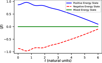
Figure 1: Time evolution of $\braket{\beta}$ for matter, antimatter, and a mixture of both. We see that $\braket{\beta}$ rapidly goes to zero for both the matter and antimatter states.

With the Rindler metric (2.16), the Rindler space Dirac inner product is

$$\Braket{\Psi_{\Omega,s,\bm{k}_{\perp}}}{\Psi_{\Omega^{\prime},s^{\prime},\bm{k}_{\perp}^{\prime}}} =\int_{\Sigma}d\Sigma_{\mu}\,\overline{\Psi}_{\Omega,s,\bm{k}_{\perp}}\gamma^{\mu}_{R}\Psi_{\Omega^{\prime},s^{\prime},\bm{k}_{\perp}^{\prime}}$$

$$=\delta(\Omega-\Omega^{\prime})\,\delta_{s,s^{\prime}}\,\delta(\bm{k}_{\perp}-\bm{k}_{\perp}^{\prime})$$ (2.44)

where $d\Sigma_{\mu}=d\Sigma n_{\mu}$ is the spatial volume element on the $v=\text{constant}$ Cauchy hypersurface $\Sigma$, $n_{\mu}$ is the unit vector normal to $\Sigma$, $s=\pm$ is the spin orientation, $\Omega=\omega c/g$ is the dimensionless frequency, $\bm{k}_{\perp}\equiv k^{a}=(k^{1},k^{2},0)$ is the wavevector perpendicular to the direction of acceleration, and $\overline{\Psi}_{\Omega,s,\bm{k}_{\perp}}=\Psi^{\dagger}_{\Omega,s,\bm{k}_{\perp}}\gamma^{0}$ is the adjoint spinor [41, 39, 34].

It is worth mentioning that had we derived Hamiltonian (2.41) in the context of a rotating frame with rotation frequency $\bm{\omega}(\tau)$, we would introduce the rotation-angular momentum coupling term $-\bm{\omega}\cdot\hat{\mathbf{J}}$ in Hamiltonian (2.41) which represents the coupling of the frame’s rotation $\bm{\omega}(\tau)$ to the observer’s total angular momentum $\hat{\mathbf{J}}=\hat{\mathbf{L}}+\mathbf{S}$ [33]. The rotation-orbital momentum coupling $\bm{\omega}\cdot\hat{\mathbf{L}}$ creates an effect very reminiscent of the Sagnac effect and induces a phase shift. This Sagnac-like effect has been experimentally verified for neutrons [44]. The rotation-spin angular momentum coupling $\bm{\omega}\cdot\mathbf{S}$ induces a phase shift smaller than the Sagnac-like effect $\bm{\omega}\cdot\hat{\mathbf{L}}$ and was recently observed in neutron interferometry experiments [45].

As mentioned previously, the choice of the Rindler coordinates will lead to slightly different forms of the Rindler Dirac Hamiltonian, and this is most pronounced when the Rindler Hamiltonian is brought to its nonrelativistic limit (see, e.g., Refs. [46, 30, 39, 34]). Our choice of Rindler coordinates (2.12) is desirable due to the fact that the observer’s local coordinate system (2.10) is what is actually used in the laboratory [33]. Most importantly, such a choice of Rindler coordinates leads to Hamiltonian (2.41) whose terms (along with the rotation-angular momentum coupling terms) have been experimentally verified for neutrons. This gives Hamiltonian (2.41), and the methodology used in its derivation, both theoretical and experimental validity in accurately modeling the behavior of a Dirac fermion in noninertial frames. Since our relativistic interpretation of the qBounce experiment uses Dirac fermions, we believe that Hamiltonian (2.41), and its linear version (2.42), is the physically most appropriate choice.

III Zitterbewegung Anti-Gravity and Ehrenfest Theorems

In this section, we derive the Ehrenfest theorems from the low energy Rindler Hamiltonian (2.43) which will be used to construct the dissipator that models entropic gravity in Sec. IV. We provide numerical simulations of the dynamics of a Dirac fermion with Hamiltonian (2.43) and its physical interpretation. In addition, we elaborate on the effect of a zitterbewegung induced anti-gravity from our simulations.

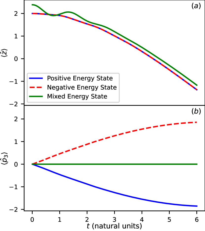
Figure 2: Time evolution of the average position (a) and momentum (b) for matter, antimatter, and a mixture of both. We see in Fig. 2 that the matter and antimatter follow the same trajectory, as prescribed by the equivalence principle.

To describe the dynamics of a Dirac fermion in a gravitational potential, it is natural to utilize the Ehrenfest theorems of the low energy Rindler Hamiltonian (2.43), which are calculated as [47]

$$\frac{d}{dt}\langle\hat{z}\rangle =\phantom{+}\Braket{\frac{\partial\hat{H}_{g}}{\partial\hat{p}_{3}}} =\phantom{+}c\Braket{\alpha_{3}},$$ (3.1)

$$\frac{d}{dt}\langle\hat{p}_{3}\rangle =-\Braket{\frac{\partial\hat{H}_{g}}{\partial\hat{z}}} =-mg\Braket{\beta}.$$ (3.2)

Unlike the nonrelativistic Ehrenfest theorems for a linear gravitational potential, Eqs. (3.1)-(3.2) depend on the $\alpha_{3}$ and $\beta$ matrices, highlighting the incorporation of antimatter free fall dynamics. To see a Dirac fermion’s spin dynamics under Eq. (2.43), we also calculate its Ehrenfest theorem. Recall that the $4\times 4$ spin observables are

$$\mathbf{S} =\frac{\hbar}{2}\bm{\Sigma}=\frac{\hbar}{2}\begin{pmatrix}\bm{\sigma}&0\\ 0&\bm{\sigma}\end{pmatrix},$$ (3.3)

which have the commutation relations

$$[\alpha_{i},S_{j}]=i\hbar\varepsilon_{ijk}\alpha_{k},\quad[\beta,S_{j}]=0,$$ (3.4)

where $\varepsilon_{ijk}$ is the Levi-Civita tensor. The first commutation relation in Eqs. (3.4) can be deduced using

$$[\sigma^{i},\sigma^{j}] =2i\varepsilon^{ijk}\sigma^{k}.$$ (3.5)

Then the Ehrenfest theorem is

$$\frac{d}{dt}\braket{S_{3}} =\frac{1}{i\hbar}\braket{[S_{3},\hat{H}_{g}]}=0,$$ (3.6)

thus the spin is conserved. We note that the full Rindler Hamiltonian (2.42) conserves spin as well.

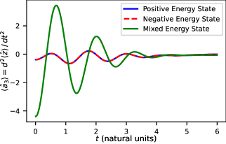
Figure 3: Time evolution of the average acceleration for matter, antimatter, and a mixture of both. We see that the acceleration for antimatter aligns with matter thus demonstrating that antimatter obeys the equivalence principle.

Using the propagator [48], we numerically solve the Dirac equation (2.43) to understand fermion’s free fall dynamics. We considered three different initial conditions of the Dirac fermion: positive energy, negative energy, and mixed energy wave packets. To get the positive energy initial state, we first take the Gaussian wave packet (see, e.g., Fig. 2(a) in [47]) centered at zero momentum and position $z_{\text{init}}=2$ (natural units $\hbar=c=m=1$ and $g=0.5$ are employed) and apply the projector [47, Eq. (37)] to eliminate negative energy components (i.e., antiparticles). The negative energy initial state, entirely made of antimatter, is obtained similarly by projecting out the positive energy components (i.e., matter). The mixed energy state, centered at the position of $z=2.38$, is made in equal proportion of matter and antimatter. Numerically obtained time evolution of $\braket{\beta}$, $\braket{\hat{z}}$, $\braket{\hat{p}_{3}}$, and $\braket{\hat{a}_{3}}=d^{2}\braket{\hat{z}}/dt^{2}$ are shown in Figs. 1, 2, 2, and 3, respectively.

In the momentum Ehrenfest theorem (3.2), the dependence on $\braket{\beta}$ superficially seems to suggest that the equivalence principle is violated. This conundrum is compounded when considering that the sign of $\braket{\beta}$ for matter and antimatter is positive and negative, respectively. However, our numerical simulations reveal that this is not the case. In Fig. 1, we see that $\braket{\beta}$ rapidly vanishes for both matter and antimatter, thus the dependence on $\braket{\beta}$ in Eq. (3.2) is effectively negligible especially given the short time scales. Additionally, in Figs. 2 and 3, we see that both matter and antimatter follow the same dynamics under the influence of gravity, thus obeying the equivalence principle.

To fully demystify the results of the mixed energy states in our simulations, we delve into the internal dynamics of the Dirac spinor itself. It is known that during time evolution, the internal degrees of freedom, i.e. matter and antimatter components, of a Dirac spinor can lead to nontrivial physical consequences [49, 50, 51]. The quantity that encodes this form of internal dynamics is the Yvon-Takabayashi angle $\theta$ [52, 53] which is defined using the pseudoscalar $\Theta$ and scalar $\Phi$ bilinear covariant quantities

$$\Theta=i\overline{\Psi}\gamma_{5}\Psi=2\varphi^{2}\sin{\theta},\quad\Phi=\overline{\Psi}\Psi=2\varphi^{2}\cos{\theta},$$ (3.7)

$$\theta=\tan^{-1}\left(\frac{\Theta}{\Phi}\right),$$ (3.8)

where the module $\varphi$ measures the density of the material distribution [54, 55, 56]. Rather than an explicit calculation, we can infer the value of the Yvon-Takabayashi angle for free-falling Dirac fermions via the Ehrenfest theorem of $\gamma_{5}$ which is

$$\frac{d}{dt}\braket{\gamma_{5}} =\frac{1}{i\hbar}\braket{[\gamma_{5},\hat{H}_{g}]}$$

$$=\frac{2m}{i\hbar}\left(\braket{c^{2}\gamma_{5}\beta}+\braket{\gamma_{5}\beta g\hat{z}}\right),$$ (3.9)

where we used

$$[\gamma_{5},\beta]=2\gamma_{5}\beta,\quad[\gamma_{5},\alpha_{i}]=0.$$ (3.10)

Since $\braket{\gamma_{5}}$ is not conserved, the Yvon-Takabayashi angle is nonzero thus the spinor will undergo jittering motion or zitterbewegung, the interference of the positive and negative energy states, even in the rest frame [56]. The zitterbewegung time scale is $t_{\text{zitt}}\sim\hbar/(2mc^{2})$, which in the adopted natural units $t_{\text{zitt}}\sim 1/2$. We note that $t_{\text{zitt}}$ is the shortest time interval for which the single-particle interpretaion of the Diract equation is valid since the corresponding uncertainty in energy $\hbar/t_{\text{zitt}}\sim 2mc^{2}$ is sufficient to create an electron-positron pair, thereby entering into the realm of quantum electrodynamics.

Figures 2 and 3 show that the position and acceleration rapidly fluctuates at the onset of free fall. These oscillations look as if the gravity and anti-gravity are interchanging. Such transient effects are due to zitterbewegung because of the time scale and the fact that the oscillations have the largest magnitude for the mixed energy state for which the particle-antiparticle interference is the strongest. We would like to name this observation as zitterbewegung-induced anti-gravity. However, Figs. 2 and 3 confirm that for longer non-transient times both matter and antimatter obey the equivalence principle.

IV Entropic Gravity For Dirac Fermions

In this section, we formulate the DFEG Lindblad master equation for Dirac fermions. We use the formalism of open quantum systems and reservoir engineering [57] to construct a reservoir that simulates entropic gravity. We demonstrate that our DFEG model for Dirac fermions is decoherence-free and provide a physical analysis of our results. In addition, we find that entropic gravity does not affect spin. The results of this section will be crucial in developing the results in Sec. VI.

Let $\hat{\rho}$ be the density matrix that represents the state of a mixture of Dirac fermions. A free-falling Dirac fermion in a linear gravitational potential

$$V(\hat{z})=\beta mg\hat{z},$$ (4.1)

is then described by the Liouville equation

$$\frac{d\hat{\rho}}{dt} =-\frac{i}{\hbar}\left[\hat{H}_{S}+\beta mg\hat{z},\hat{\rho}\right],$$ (4.2)

$$\hat{H}_{S} =c\alpha_{3}\hat{p}_{3}+\beta mc^{2},$$ (4.3)

and its dynamics follow the free-fall Ehrenfest theorems (3.1)-(3.2) which can be shown using Eq. (4.2) and the density matrix expectation value

$$\langle\hat{O}\rangle=\text{Tr}\left[\hat{O}\hat{\rho}\right],$$ (4.4)

where $\hat{O}\equiv O(\hat{z},\hat{p}_{3})$ is an arbitrary observable. Eq. (4.2) is the conservative gravity master equation for Dirac fermions. Quantum coherence is encapsulated by the purity $\text{Tr}[\hat{\rho}^{2}]$, which is being conserved by Eq. (4.2).

There exists an infinite number of master equations that satisfy Eqs. (3.1)-(3.2). This means that we can find a master equation that mimics conservative gravity by utilizing a dissipator instead of using a potential. By carefully engineering an environment, a quantum system can obey the dynamics governed by the Ehrenfest-like equations [6]

$$\frac{d}{dt}\braket{\hat{z}}=\braket{A(\hat{p}_{3})},\quad\frac{d}{dt}\braket{\hat{p}_{3}}=\braket{B(\hat{z})}.$$ (4.5)

For our purpose of modeling entropic gravity, we wish to engineer an environment that simulates the linear gravitational potential (4.1) and follows the dynamics according to Eqs. (3.1)-(3.2). To achieve that, the paradigm of Operational Dynamical Modeling (ODM) [58] for spin-$1/2$ relativistic particles [47] is to be employed.

We use the simplest scenario of a single dissipator coupled to the closed system of a free Dirac fermion. In the formalism of open quantum systems theory, the Dirac fermion’s density matrix $\hat{\rho}$ evolves according to the Lindblad master equation [59]

$$\frac{d\hat{\rho}}{dt} =-\frac{i}{\hbar}\left[\hat{H}_{S},\hat{\rho}\right]+\mathcal{D}[\hat{\rho}],$$ (4.6)

$$\mathcal{D}[\hat{\rho}] =\frac{\sigma}{\hbar}\left(\hat{A}\hat{\rho}\hat{A}^{\dagger}-\frac{1}{2}\{\hat{A}^{\dagger}\hat{A},\hat{\rho}\}\right).$$ (4.7)

where the free parameter $\sigma\geq 0$ is the dimensionless coupling constant that quantifies the coupling strength and $\hat{A}\equiv A(\hat{z},\hat{p}_{3})$ is the unknown jump operator [60, 57, 61]. To find the correct choice of $\hat{A}$ such that master equation (4.6) simulates an entropic gravity environment, we insert $\hat{z}$ and $\hat{p}_{3}$ into the Ehrenfest equation

$$\frac{d}{dt}\langle\hat{O}\rangle =\frac{i}{\hbar}\Braket{\left[\hat{H}_{S},\hat{O}\right]}+\langle\mathcal{D}^{\dagger}[\hat{O}]\rangle,$$

$$\langle\mathcal{D}^{\dagger}[\hat{O}]\rangle =\frac{\sigma}{\hbar}\text{Tr}\left[\left(\hat{A}^{\dagger}\hat{O}\hat{A}-\frac{1}{2}\{\hat{A}^{\dagger}\hat{A},\hat{O}\}\right)\hat{\rho}\right],$$ (4.8)

and set them equal to Eqs. (3.1) and (3.2), respectively, which yields

$$\text{Tr}\left[\left(\hat{A}^{\dagger}\frac{\partial\hat{A}}{\partial\hat{p}_{3}}-\frac{\partial\hat{A}^{\dagger}}{\partial\hat{p}_{3}}\hat{A}\right)\hat{\rho}\right] =0,$$ (4.9)

$$\text{Tr}\left[\left(\hat{A}^{\dagger}\frac{\partial\hat{A}}{\partial\hat{z}}-\frac{\partial\hat{A}^{\dagger}}{\partial\hat{z}}\hat{A}\right)\hat{\rho}\right] =-\frac{2img}{\sigma}\text{Tr}\left[\beta\hat{\rho}\right],$$ (4.10)

where we have used the cyclic invariance property of the trace operation and

$$[A(\hat{z},\hat{p}_{3}),\hat{z}]=-i\hbar\frac{\partial\hat{A}}{\partial\hat{p}_{3}},\quad[A(\hat{z},\hat{p}_{3}),\hat{p}_{3}]=i\hbar\frac{\partial\hat{A}}{\partial\hat{z}}.$$ (4.11)

We demand that identities Eqs. (4.9)-(4.10) hold for any arbitrary initial state, thus we drop the averaging and get the following constraint equations for $\hat{A}$

$$\hat{A}^{\dagger}\frac{\partial\hat{A}}{\partial\hat{p}_{3}}-\frac{\partial\hat{A}^{\dagger}}{\partial\hat{p}_{3}}\hat{A} =0,$$ (4.12)

$$\hat{A}^{\dagger}\frac{\partial\hat{A}}{\partial\hat{z}}-\frac{\partial\hat{A}^{\dagger}}{\partial\hat{z}}\hat{A} =-\frac{2img}{\sigma}\beta.$$ (4.13)

Any jump operator $\hat{A}$ that satisfies Eqs. (4.12)-(4.13) will yield Eqs. (3.1)-(3.2) when using Eq. (4.6), thus creating an entropic gravity environment that simulates the free-fall dynamics of conservative gravity.

Our choice of $\hat{A}$ is narrowed by the fact that $\hat{A}$ is not unique. Other than satisfying Eqs. (4.12)-(4.13), the choice of jump operator $\hat{A}$ must yield a master equation that is translationally invariant. This would make the master equation obey the strong equivalence principle [40] since the dynamics induced by the homogeneous gravitational field are independent of the choice of origin. According to Refs. [62, 63, 64, 65, 66, 67], the following form is guaranteed to be translationary invariant

$$A(\hat{z},\hat{p}_{3}) =e^{-iC\hat{z}}h(\hat{p}_{3}),\quad C^{\dagger}=C,$$ (4.14)

where $C$ is a Hermitian matrix. Inserting the ansatz (4.14) into Eqs. (4.12)-(4.13) yields

$$\hat{h}^{\dagger}\frac{d\hat{h}}{d\hat{p}_{3}}-\frac{d\hat{h}^{\dagger}}{d\hat{p}_{3}}\hat{h} =0,$$ (4.15)

$$\hat{h}^{\dagger}C\hat{h} =\frac{mg}{\sigma}\beta.$$ (4.16)

There are many ways to satisfy Eqs. (4.15)-(4.16) but for our work, we choose $h(\hat{p}_{3})=\sqrt{mgx_{0}}\mathbbm{1}_{4}$ such that $\hat{h}$ is a constant matrix. The value of the characteristic length $x_{0}$ will be determined in Sec. VII. Then the Hermitian matrix (4.16) is

$$C=\frac{1}{x_{0}\sigma}\beta,$$ (4.17)

and the jump operator is

$$A(\hat{z},\hat{p}_{3}) \equiv A(\hat{z})=\sqrt{mgx_{0}}e^{-i\beta\hat{z}/(x_{0}\sigma)}.$$ (4.18)

Finally, the DFEG equation for Dirac fermions is

$$\frac{d\hat{\rho}}{dt} =-\frac{i}{\hbar}\left[c\alpha_{3}\hat{p}_{3}+\beta mc^{2},\hat{\rho}\right]+\mathcal{D}[\hat{\rho}],$$ (4.19)

$$\mathcal{D}[\hat{\rho}] =\frac{mgx_{0}\sigma}{\hbar}\left(e^{-i\beta\hat{z}/(x_{0}\sigma)}\hat{\rho}e^{+i\beta\hat{z}/(x_{0}\sigma)}-\hat{\rho}\right).$$ (4.20)

We shall refer to master equation (4.19) as the Dirac DFEG master equation or model. As mentioned before, the Dirac DFEG model (4.19) is translationally invariant hence it obeys the strong equivalence principle.

To verify that our Dirac DFEG model (4.19) reproduces the conservative gravity model (4.2) in the strong coupling limit $\sigma\rightarrow\infty$, we expand the exponential in dissipator (4.20) using the Baker-Campbell-Hausdorff (BCH) formula in the limit $\sigma\rightarrow\infty$ to get

$$\frac{d\hat{\rho}}{dt} =-\frac{i}{\hbar}\left[c\alpha_{3}\hat{p}_{3}+\beta mc^{2}+\beta mg\hat{z},\hat{\rho}\right]$$

$$+\frac{mg}{x_{0}\hbar\sigma}\left(\hat{z}\beta\hat{\rho}\beta\hat{z}-\frac{1}{2}\{\hat{z}^{2},\hat{\rho}\}\right)+O(\sigma^{-2}).$$ (4.21)

The $O(\sigma^{-2})$ term in Eq. (4.21) quickly vanishes thus our Dirac DFEG model (4.19) reproduces the dynamics of a Dirac fermion subject to a linear gravitational potential, namely, master equation (4.2).

As proved in Appendix A, the purity equation for the Dirac DFEG model in the strong coupling limit (4.21) is

$$\frac{d}{dt}\text{Tr}[\hat{\rho}^{2}] =-\frac{2mg}{x_{0}\hbar\sigma}\text{Tr}\left[\hat{\rho}^{2}\hat{z}^{2}-(\hat{\rho}\beta\hat{z})^{2}\right]+O(\sigma^{-2}),$$ (4.22)

with $\text{Tr}[\hat{\rho}^{2}\hat{z}^{2}-(\hat{\rho}\beta\hat{z})^{2}]\geq 0$. Thus Eq. (4.22) monotonically decreases as $\sigma\rightarrow\infty$ and larger $\sigma$ values, i.e. stronger coupling, can be chosen to preserve more purity leading to quantum coherence being maintained. Therefore, our Dirac DFEG model lives up to its namesake and is decoherence-free thus the argument that entropic gravity destroys quantum coherence is refuted for Dirac fermions.

If we insert the low energy Hamiltonian (2.43) into the Dirac DFEG equation in the strong coupling limit (4.21), we get

$$\frac{d}{dt}\braket{\hat{H}_{g}} =-\frac{2mgc}{x_{0}\hbar\sigma}\Braket{\alpha_{3}\hat{z}\hat{p}_{3}\hat{z}}+O(\sigma^{-2}).$$ (4.23)

We see that the expected energy rate is dependent on the state due to the position and momentum operators present in (4.23). This is in stark contrast to the nonrelativistic DFEG model’s constant expected rate of energy change $g\hbar/(2x_{0}\sigma)$ [6, Eq. (24)].

To see the spin dynamics in our entropic gravity model (4.19), we calculate its Ehrenfest theorem. We see that inserting the spin (3.3) into dissipator (4.20) yields

$$\mathcal{D}[S_{j}]=\mathcal{D}^{\dagger}[S_{j}]=0,$$ (4.24)

where we have used Eqs. (3.4), so the spin Ehrenfest theorems are

$$\frac{d}{dt}\Braket{S_{j}} =\frac{i}{\hbar}\Braket{\left[c\alpha_{3}\hat{p}_{3}+\beta mc^{2},S_{j}\right]}+\Braket{\mathcal{D}^{\dagger}[S_{j}]}$$

$$=-\Braket{\varepsilon_{3jk}c\alpha_{k}\hat{p}_{3}},$$ (4.25)

or explicitly,

$$\frac{d}{dt}\Braket{S_{1}}=-\Braket{c\alpha_{2}\hat{p}_{3}},\quad\frac{d}{dt}\Braket{S_{2}}=\Braket{c\alpha_{1}\hat{p}_{3}},$$ (4.26)

$$\frac{d}{dt}\Braket{S_{3}}=0.$$ (4.27)

We see from Eqs. (4.24) and (4.27) that the dissipator (4.20) preserves the spin along the direction of the acceleration. Thus our entropic gravity model implies that the free-fall dynamics of spin-$1/2$ Dirac fermions are the same as spinless particles therefore our model does not conflict with the equivalence principle. This is in agreement with recent experiments of the equivalence principle on spin-1/2 atoms which have demonstrated that an atom’s spin [68] and its orientation [69] does not affect its free-fall dynamics, based on current sensitivity levels.

We end this section by pointing out that while relativistic dissipative phenomena exist, there currently does not exist an accepted relativistic Lindblad master equation. Díosi [70] argued that it might be impossible to construct a relativistic Lindblad master equation. Nevertheless, there have been several proposals, such as covariant density matrix formulations [71, 48], which have seen varying degrees of success in formulating relativistic open quantum systems. Since we are working in the low energy regime by using Hamiltonian (2.43), our Dirac DFEG model (4.19) is a low energy model and is within the range of applicability of nonrelativistic open quantum systems. Therefore, our model avoids the ambiguity of relativistic open quantum systems. We will see later in Sec. VII that our model (4.19) successfully reduces to the nonrelativistic DFEG model which makes our master equation (4.19) a satisfactory, ad-hoc model for Dirac fermions.

V Boundary Condition of Bouncing Dirac Fermion

In this section, we choose the boundary condition from Ref. [28] and present its re-derivation, which will be crucial in modeling the relativistic qBounce experiment in Sec. VI. We give the rationale for such a choice along with some brief insight into the difficulty of imposing boundary conditions on the Dirac equation.

The boundary condition, modeling the vibrating mirror in the qBounce experiment, must satisfy two criteria if we are to relativistically generalize the qBounce Hamiltonian in [6]: $(1)$ the (relativistic) boundary condition should reduce to $J^{3}\lvert_{u=u_{0}}=0$, i.e., a vanishing probability current at the mirror’s location $u_{0}$ ensuring that the Dirac fermions are reflected after hitting the mirror; and $(2)$ the (relativistic) boundary condition should reduce to the Dirichlet condition in the nonrelativistic limit.

Choosing appropriate boundary conditions that satisfy the criteria is rather complicated. The most logical choice is to utilize the Dirichlet condition, as is done for the nonrelativistic linear gravitational potential [29] and the Rindler space Klein-Gordon equation [72], but imposing the Dirichlet condition on the Rindler Hamiltonian’s (2.39) eigenspinors (Eq. (B22) in Appendix B) leads to the trivial solution when calculating the energy levels [30, 28], which is clearly undesirable. Treading around this problem and directly using the vanishing probability current condition $J^{3}\lvert_{u=u_{0}}=0$ on the eigenspinors leads to the trivial solution as well [30, 28]. The commonly used MIT boundary condition [73] satisfies our first criterion and also leads to energy quantization for the Rindler Hamiltonian (2.39) (see Ref. [30] and Appendix B for the energy levels) but does not reduce to the Dirichlet condition in the nonrelativistic limit [74]. Thus we rule out the MIT condition.

To avoid these issues and satisfy our criteria, we elect to utilize the boundary condition in [28] where we model the mirror as a scalar potential

$$\phi(z) =\begin{cases}0,&z>0,\\ V_{0}\gg mc^{2},&z\leq 0,\end{cases}$$ (5.1)

or in Rindler coordinates,

$$\phi(u) =\begin{cases}0,&u>u_{0},\\ V_{0}\gg mc^{2},&u\leq u_{0},\end{cases}$$ (5.2)

where $u_{0}=c^{2}/g$ is the mirror’s location. Incorporating potential (5.1) essentially amounts to the replacement

$$mc^{2}\rightarrow\overline{m}c^{2}=mc^{2}+V_{0},$$ (5.3)

at the level of the Lagrangian [28] leading to the Rindler Hamiltonian (2.37) to instead use the mass term (5.3). We now closely follow Ref. [28] and rederive the boundary condition that we will impose on the spinors of the Rindler Hamiltonian (2.37).

We begin with the derivation of a modified form of the Rindler Hamiltonian (2.37) from which we find the differential equation for the spinor. For any positive frequency, spin-dependent spinor $\Psi_{s}$ that satisfies Hamiltonian (2.37), we use the modified plane wave ansatz [28]

$$\Psi_{s}(x) =e^{-i\Omega v}e^{ikx}u^{-1/2}\psi_{s}(u),\quad\Omega>0,$$ (5.4)

$$x \equiv x^{\mu}=(v,x^{1},x^{2},u),$$

$$\mathbf{x}\equiv x^{a} =(x^{1},x^{2},u),\quad a=1,2,$$

$$kx \equiv\bm{k}_{\perp}\cdot\mathbf{x}=-k_{a}x^{a}=k^{1}x^{1}+k^{2}x^{2},$$

$$k =\left\lvert\bm{k}_{\perp}\right\rvert=\sqrt{(k^{1})^{2}+(k^{2})^{2}},$$

where $\Omega=\omega c/g$ is the dimensionless frequency. Note that ansatz (5.4) differs from the usual plane wave ansatz (B3) in Appendix B. Inserting ansatz (5.4) into Eq. (2.33) yields

$$\left[\Omega\gamma^{0}+\not{k}u+iu\gamma^{3}\partial_{u}-\overline{\ell}u\right]\psi_{s}=0,$$ (5.5)

where $\not{k}=k_{a}\gamma^{a}=-(k^{1}\gamma^{1}+k^{2}\gamma^{2})$ and $\overline{\ell}=\overline{m}c/\hbar$. Then we use another ansatz that decomposes the spatial spinor $\psi_{s}$ as

$$\psi_{s}(u) =F(u)U_{s}+G(u)\gamma^{3}U_{s},$$ (5.6)

where the spin-dependent spinor $U_{s}$ obeys

$$U^{\dagger}_{s}U_{s^{\prime}}=\delta_{s,s^{\prime}},\quad\gamma^{0}U_{s}=U_{s},\quad\hat{\not{k}}\gamma^{3}U_{s}=isU_{s},$$ (5.7)

and $\hat{\not{k}}=\not{k}/k$ [28]. Note that Eqs. (5.7) also imply that

$$U^{\dagger}_{s}\gamma^{3}U_{s}=0.$$ (5.8)

Using the ansatz decomposition (5.6) on Eq. (5.5) then decouples Eq. (5.5) into

$$\begin{cases}\phantom{+}D_{-}F-iksG-i(\partial_{u}G)=0,\\ -D_{+}G-iksF+i(\partial_{u}F)=0,\end{cases}$$ (5.9)

where we have used the linear independence of $U_{s}$ and $\gamma^{3}U_{s}$ to decouple $F$ and $G$ and

$$D_{\pm} =\frac{\Omega}{u}\pm\overline{\ell}.$$ (5.10)

We can use the first and second equations from Eqs. (5.9) to get

$$F =\frac{i}{D_{-}}(\partial_{u}+ks)G,$$ (5.11)

$$G =\frac{i}{D_{+}}(\partial_{u}-ks)F,$$ (5.12)

respectively, thus we can find $G$ from $F$ and vice versa. We choose to focus on $F$ and use identity (5.12) on the first equation in Eqs. (5.9) to get

$$\left[\partial^{2}_{u}-\frac{(\partial_{u}D_{+})}{D_{+}}(\partial_{u}-ks)+D_{+}D_{-}-k^{2}s^{2}\right]F=0,$$ (5.13)

which we simplify further using

$$F(u) =D^{1/2}_{+}f(u),$$ (5.14)

which leads to our desired differential equation

$$\left[\partial^{2}_{u}+D_{+}D_{-}-k^{2}s^{2}+\frac{(\partial_{u}D_{+})}{D_{+}}ks+\frac{(\partial^{2}_{u}D_{+})}{2D_{+}}\right.$$

$$\left.-\frac{3(\partial_{u}D_{+})^{2}}{4D^{2}_{+}}\right]f=0.$$ (5.15)

With Eq. (5.15), we can now find the boundary condition for spinor (5.6) by analyzing the asymptotic behavior of the function $f(u)$ based on the mirror potential (5.2). In the region $u>u_{0}$, $\phi(u)=0$ so $\overline{m}=m$ and we are left with the Rindler Hamiltonian (2.37) thus there are no continuity rules to impose on spinor (5.6). In the region $u<u_{0}$, $\phi(u)=V_{0}\gg mc^{2}$ so if we take the limit $V_{0}\rightarrow\infty$, we have

$$D_{\pm} \approx\pm\frac{V_{0}}{\hbar c},$$ (5.16)

which leads to Eq. (5.15) asymptotically reducing to

$$(\partial^{2}_{u}f)\approx\left(\frac{V_{0}}{\hbar c}\right)^{2}f.$$ (5.17)

Solving Eq. (5.17) yields

$$f(u)\approx Ne^{V_{0}u/\hbar c},$$ (5.18)

where $N$ is a normalization constant. Then we use identities (5.14) and (5.12) to find that

$$F(u)\approx Ne^{V_{0}u/\hbar c},\quad G(u)\approx iNe^{V_{0}u/\hbar c},$$ (5.19)

respectively, in the $u<u_{0}$ region. The wave function must be continuous at the mirror’s location $u=u_{0}$ which we can impose by assuming from Eq. (5.19) the Robin boundary condition

$$F\Big{\lvert}_{u=u_{0}} =-iG\Big{\lvert}_{u=u_{0}}.$$ (5.20)

Thus we finally have our boundary condition for the wave function. To explicitly see why condition (5.20) is a Robin condition, we use identities (5.11)-(5.12) to rewrite condition (5.20) for $F$ and $G$ as

$$(D_{+}+ks)F\Big{\lvert}_{u=u_{0}} =(\partial_{u}F)\Big{\lvert}_{u=u_{0}},$$ (5.21)

$$-(D_{-}+ks)G\Big{\lvert}_{u=u_{0}} =(\partial_{u}G)\Big{\lvert}_{u=u_{0}},$$ (5.22)

respectively.

For subsequent sections, it would prove far more fruitful to have boundary condition (5.20) in spinor form $\Psi_{s}$. To achieve this, we simply impose condition (5.20) on the decomposition ansatz (5.6) and use Eqs. (5.7) to get

$$i\gamma^{3}\Psi_{s}\Big{\lvert}_{u=u_{0}} =\Psi_{s}\Big{\lvert}_{u=u_{0}},$$ (5.23)

which is the MIT boundary condition for chiral angle $\theta_{\text{M}}=0$ [73, 75]. The difference between the MIT condition and condition (5.23) is that the MIT condition focuses only on the spinor $\Psi_{s}$, making no explicit assumption as to the form of the spinor, while our condition (5.23) focuses on the functions $F$ and $G$ that the spinor $\Psi_{s}$ is composed of.

We now verify that boundary condition (5.23) satisfies our criteria. To test the first criterion, we calculate the probability current which is

$$J^{3}\Big{\lvert}_{u=u_{0}} =\overline{\Psi}_{s}\gamma^{3}\Psi_{s}\Big{\lvert}_{u=u_{0}}$$

$$=\frac{i}{D_{+}}(F(\partial_{u}F)^{\ast}-F^{\ast}(\partial_{u}F))\Big{\lvert}_{u=u_{0}}.$$ (5.24)

Now $F$ and $(\partial_{u}F)$ are determined up to an arbitrary complex coefficient thus we choose them to be real functions which make the probability current (5.24) vanish at the boundary [28]

$$J^{3}\Big{\lvert}_{u=u_{0}} =\overline{\Psi}_{s}\gamma^{3}\Psi_{s}\Big{\lvert}_{u=u_{0}}=0.$$ (5.25)

We can also prove Eq. (5.25) by using condition (5.23), and its adjoint form

$$-i\overline{\Psi}_{s}\gamma^{3}\Big{\lvert}_{u=u_{0}} =\overline{\Psi}_{s}\Big{\lvert}_{u=u_{0}},$$ (5.26)

to get [30]

$$J^{3}\Big{\lvert}_{u=u_{0}} =\overline{\Psi}_{s}\gamma^{3}\Psi_{s}\Big{\lvert}_{u=u_{0}}$$

$$=\overline{\Psi}_{s}\Psi_{s}\Big{\lvert}_{u=u_{0}}=-\overline{\Psi}_{s}\Psi_{s}\Big{\lvert}_{u=u_{0}}=0.$$ (5.27)

Thus our first criterion is satisfied. In the nonrelativistic limit, we can expand the exponentials in Eqs. (5.19) up to $O(c^{-1})$ then impose condition (5.20) to get

$$F\Big{\lvert}_{u=u_{0}}\approx N=-iN\approx G\Big{\lvert}_{u=u_{0}},$$ (5.28)

which implies that [28]

$$F\Big{\lvert}_{u=u_{0}}\approx 0,\quad G\Big{\lvert}_{u=u_{0}}\approx 0.$$ (5.29)

In spinor form, conditions (5.29) trivially lead to

$$\Psi_{s}\Big{\lvert}_{u=u_{0}}\approx 0,$$ (5.30)

thus boundary condition (5.20) nonrelativistically reduces to the Dirichlet condition, satisfying our second criterion.

We now derive a crucial identity that will be used in the next section. We take the first derivative of ansatz (5.6) and impose the boundary condition (5.20) to get

$$(\partial_{u}\psi_{s})\Big{\lvert}_{u=u_{0}} =(\partial_{u}F)U_{s}+(\partial_{u}G)\gamma^{3}U_{s}\Big{\lvert}_{u=u_{0}}$$

$$=\Omega_{u}\left(FU_{s}-G\gamma^{3}U_{s}\right)+\ell\psi_{s}\Big{\lvert}_{u=u_{0}}$$

$$=\Omega_{u}\left(F\gamma^{0}U_{s}-G\gamma^{3}(\gamma^{0})^{2}U_{s}\right)+\ell\psi_{s}\Big{\lvert}_{u=u_{0}}$$

$$=\left(\Omega_{u}\gamma^{0}+\ell\right)\psi_{s}\Big{\lvert}_{u=u_{0}},$$ (5.31)

$$\Omega_{u} =\left(\Omega u^{-1}+ks\right),$$ (5.32)

where we used identities (5.11)-(5.12), $(\gamma^{0})^{2}=1$, and (5.7) in the second, third, and fourth equalities, respectively. Then we have

$$\overline{\psi}_{s}(\partial_{u}\psi_{s})\Big{\lvert}_{u=u_{0}} =\overline{\psi}_{s}\left(\Omega_{u}\gamma^{0}+\ell\right)\psi_{s}\Big{\lvert}_{u=u_{0}}$$

$$=(\partial_{u}\overline{\psi}_{s})\psi_{s}\Big{\lvert}_{u=u_{0}},$$ (5.33)

therefore

$$(\partial_{u}\overline{\Psi}_{s})\Psi_{s}\Big{\lvert}_{u=u_{0}}=\overline{\Psi}_{s}(\partial_{u}\Psi_{s})\Big{\lvert}_{u=u_{0}},$$ (5.34)

or equivalently in the observer’s coordinates,

$$(\partial_{3}\overline{\Psi}_{s})\Psi_{s}\Big{\lvert}_{z=0}=\overline{\Psi}_{s}(\partial_{3}\Psi_{s})\Big{\lvert}_{z=0}.$$ (5.35)

VI Relativistic qBounce Hamiltonian

In this section, we relativistically model qBounce experiment by using the boundary condition from Sec. V to find the surface term that arises from the Rindler Hamiltonian’s Ehrenfest theorems. Although we will ultimately use the low energy Hamiltonian (2.43), we first use the linear high energy Rindler Hamiltonian (2.39) to not miss any low-order terms. We will remove the high-order terms and modify the low energy Hamiltonian (2.43) with the surface term. Then, we will apply the results of Sec. IV to formulate the relativistic master equations that reproduce the qBounce experiment.

We follow the methodology in [6] and modify the Ehrenfest theorems of the high-energy, linear Rindler Hamiltonian (2.39). We require a temporal variable which we easily identify from Eqs. (2.12) as $v$, so the Ehrenfest theorems for the Rindler position and momentum operators (2.35) are

$$\frac{d}{dv}\langle\hat{u}\rangle=\langle\alpha_{3}\hat{u}\rangle,\quad\frac{d}{dv}\langle\hat{p}_{u}\rangle=-\langle\alpha_{3}\hat{p}_{u}\rangle-mc\langle\beta\rangle,$$ (6.1)

respectively. However, the above equations do not incorporate the contribution of boundary condition (5.20), i.e. the vibrating mirror, so we integrate by parts with the Dirac inner product (2.44) to find the surface term generated by condition (5.20). Following this prescription for the Rindler momentum operator $\hat{p}_{u}$ yields

$$\frac{d}{dv}\langle\hat{p}_{u}\rangle =-\langle\alpha_{3}\hat{p}_{u}\rangle-mc\langle\beta\rangle-\frac{i\hbar c^{2}}{g}\overline{\Psi}\gamma^{3}(\partial_{u}\Psi)\Big{\lvert}_{u=u_{0}}$$

$$=-\langle\alpha_{3}\hat{p}_{u}\rangle-mc\langle\beta\rangle+\frac{\hbar c^{2}}{g}\overline{\Psi}(\partial_{u}\Psi)\Big{\lvert}_{u=u_{0}}$$

$$=-\langle\alpha_{3}\hat{p}_{u}\rangle-mc\langle\beta\rangle+\Braket{f_{R}(\hat{u})},$$ (6.2)

where we used condition (5.23) in the second equality and have identified the Rindler statistical force

$$\Braket{f_{R}(\hat{u})} =\frac{\hbar c^{2}}{2g}\Braket{\beta\delta^{\prime}(\hat{u}-u_{0})},$$ (6.3)

where $u_{0}=c^{2}/g$, as the surface term that arises from boundary condition (5.20). The $1/2$ factor comes from identity (5.34) and the Dirac delta function $\delta(x)$ is defined as

$$\int^{\infty}_{-\infty}dx\,\delta^{(n)}(x-x^{\prime})f(x) =(-1)^{n}f^{(n)}(x^{\prime}).$$ (6.4)

Note that we have suppressed the spin subscript $s$. Similar calculations for the Rindler position operator $\hat{u}$ yields

$$\frac{d}{dv}\langle\hat{u}\rangle =\langle\alpha_{3}\hat{u}\rangle+\left(\frac{c^{4}}{g^{2}}J^{3}\right)\Big{\lvert}_{u=u_{0}}=\langle\alpha_{3}\hat{u}\rangle,$$ (6.5)

where we used the vanishing probability current condition (5.25). Thus the Ehrenfest theorems for the Rindler position and momentum operators with boundary condition (5.20) are

$$\frac{d}{dv}\langle\hat{u}\rangle =\phantom{+}\langle\alpha_{3}\hat{u}\rangle,$$ (6.6)

$$\frac{d}{dv}\langle\hat{p}_{u}\rangle =-\langle\alpha_{3}\hat{p}_{u}\rangle-mc\langle\beta\rangle+\Braket{f_{R}(\hat{u})},$$ (6.7)

respectively. Using Eqs. (2.12) on Eqs. (6.6)-(6.7) yields the Ehrenfest theorems in the observer’s local coordinates $(t,z)$

$$\frac{d}{dt}\langle\hat{z}\rangle =\phantom{+}\frac{g}{c}\langle\alpha_{3}\hat{z}\rangle+c\langle\alpha_{3}\rangle,$$ (6.8)

$$\frac{d}{dt}\langle\hat{p}_{3}\rangle =-\frac{g}{c}\langle\alpha_{3}\hat{p}_{3}\rangle-mg\langle\beta\rangle+\Braket{f_{S}(\hat{z})},$$ (6.9)

which, in the low energy regime, reduces to

$$\frac{d}{dt}\langle\hat{z}\rangle =\phantom{+}c\langle\alpha_{3}\rangle,$$ (6.10)

$$\frac{d}{dt}\langle\hat{p}_{3}\rangle =-mg\langle\beta\rangle+\Braket{f_{S}(\hat{z})},$$ (6.11)

where

$$\braket{f_{S}(\hat{z})} =\frac{\hbar c}{2}\Braket{\beta\delta^{\prime}(\hat{z})},$$ (6.12)

is the surface term (6.3) in the observer’s coordinates.

We add the surface term (6.12) to the system Hamiltonian (4.3) to get the relativistic qBounce Hamiltonian

$$\hat{H}_{q} =c\alpha_{3}\hat{p}_{3}+\beta mc^{2}+V_{q}(\hat{z})-\frac{\hbar c}{2}\beta\delta(\hat{z}),$$ (6.13)

where

$$V_{q}(\hat{z}) =\begin{cases}\beta mg\hat{z},\quad&\text{conservative gravity},\\ 0,\quad&\text{entropic gravity}.\end{cases}$$ (6.14)

To make the boundary oscillate, we add a sinusoidal term in the argument of the delta function as follows

$$\hat{H}_{q} =c\alpha_{3}\hat{p}_{3}+\beta mc^{2}+V_{q}(\hat{z})-\frac{\hbar c}{2}\beta\delta(\hat{z}-a_{m}\sin{\omega_{m}t}),$$ (6.15)

where $a_{m}$ and $\omega_{m}$ are the vibrating mirror’s oscillation strength and frequency, respectively. We can now apply the Dirac DFEG model (4.19) to Hamiltonian (6.15) to get the relativistic qBounce experiment’s master equations for conservative and entropic gravity

$$\frac{d\hat{\rho}}{dt} =-\frac{i}{\hbar}\left[\vphantom{\frac{1}{1}}c\alpha_{3}\hat{p}_{3}+\beta mc^{2}+\beta mg\hat{z}\right.$$

$$\left.-\frac{\hbar c}{2}\beta\delta(\hat{z}-a_{m}\sin{\omega_{m}t}),\hat{\rho}\right],$$ (6.16)

$$\frac{d\hat{\rho}}{dt} =-\frac{i}{\hbar}\left[\vphantom{\frac{1}{1}}c\alpha_{3}\hat{p}_{3}+\beta mc^{2}\right.$$

$$\left.-\frac{\hbar c}{2}\beta\delta(\hat{z}-a_{m}\sin{\omega_{m}t}),\hat{\rho}\right]+\mathcal{D}[\hat{\rho}],$$ (6.17)

respectively.

Compared to the qBounce Hamiltonian’s boundary term in [6, Eq. (16)] which was proportional to the first derivative of the Dirac delta function, the relativistic Hamiltonian’s (6.15) boundary term is $\propto$ the Dirac delta function. In addition, the appearance of the $\beta$ matrix captures the effect of the mirror on both matter and antimatter as well.

VII Nonrelativistic Limit

With our master equations fully developed, we now present the nonrelativistic limit of our results. We use the Foldy-Wouthysen (FW) transformation [76] to find the nonrelativistic approximation of our Hamiltonians then use the FW Hamiltonians to construct their corresponding nonrelativistic master equations.

VII.1 Hamiltonian

We begin with a brief overview of the FW transformation. Let $\Psi(\mathbf{x},t)$ be an arbitrary Dirac spinor that satisfies the general Dirac equation

$$i\hbar\partial_{t}\Psi =\hat{H}_{\mathbf{D}}\Psi,$$ (7.1)

$$\hat{H}_{\mathbf{D}} =c\bm{\alpha}\cdot\hat{\mathbf{p}}+\beta mc^{2}+V_{D}(\hat{\mathbf{x}})+K(\hat{\mathbf{p}}),$$ (7.2)

where $V_{D}(\hat{\mathbf{x}})$ and $K(\hat{\mathbf{p}})$ are matrix-valued functions of operators $\hat{\mathbf{x}}$ and $\hat{\mathbf{p}}$, respectively. Following the standard convention, we define the even and odd components of Hamiltonian (7.2) as [76, 77]

$$\hat{\mathcal{E}}=\frac{1}{2}(\hat{H}_{\mathbf{D}}+\beta\hat{H}_{\mathbf{D}}\beta),\quad\hat{\mathcal{O}}=\frac{1}{2}(\hat{H}_{\mathbf{D}}-\beta\hat{H}_{\mathbf{D}}\beta),$$ (7.3)

respectively, where

$$[\beta,\hat{\mathcal{E}}]=\{\beta,\hat{\mathcal{O}}\}=0.$$ (7.4)

We also define the following operators

$$\hat{S}_{1}=-\frac{i\beta\hat{\mathcal{O}}}{2mc^{2}},\quad\hat{U}_{1}=e^{i\hat{S}_{1}},$$ (7.5)

which are Hermitian and unitary, respectively, where the subscript denotes the number of FW transformations applied. Then Hamiltonian (7.2) can be written as

$$\hat{H}_{\mathbf{D}}=\hat{\mathcal{O}}+\hat{\mathcal{E}},$$ (7.6)

and applying the first FW transformation on Hamiltonian (7.6) yields [76]

$$\hat{H}_{1} =\hat{U}_{1}\hat{H}_{\mathbf{D}}\hat{U}^{\dagger}_{1},$$ (7.7)

$$\Psi_{1} =\hat{U}_{1}\Psi,$$ (7.8)

which turns Eq. (7.1) into

$$i\hbar\partial_{t}\Psi_{1} =\hat{H}_{1}\Psi_{1}.$$ (7.9)

We can then evaluate Eq. (7.7) up to a desired order via the BCH expansion and subsequent FW transformations can be performed using

$$\hat{S}_{n}=-\frac{i\beta\hat{\mathcal{O}}_{n-1}}{2mc^{2}},\quad\hat{U}_{n}=e^{i\hat{S}_{n}},$$ (7.10)

which yields

$$i\hbar\partial_{t}\Psi_{FW} =\hat{H}_{FW}\Psi_{FW},$$ (7.11)

$$\hat{H}_{FW} \equiv\hat{H}_{n}=\hat{U}_{n}\hat{H}_{n-1}\hat{U}^{\dagger}_{n},$$ (7.12)

$$\Psi_{FW} \equiv\Psi_{n}=\hat{U}_{n}\Psi_{n-1},$$ (7.13)

where $n=1,2,\ldots$. For most of our Hamiltonians, we require three FW transformations thus applying the FW transformation three times to remove all odd operators yields [33]

$$\hat{H}_{FW} \equiv\hat{H}_{3}=\beta\left(mc^{2}+\frac{\hat{\mathcal{O}}^{2}}{2mc^{2}}-\frac{\hat{\mathcal{O}}^{4}}{8m^{3}c^{6}}\right)+\hat{\mathcal{E}}$$

$$-\frac{1}{8m^{2}c^{4}}[\hat{\mathcal{O}},[\hat{\mathcal{O}},\hat{\mathcal{E}}]],$$ (7.14)

which turns Eq. (7.1) into

$$i\hbar\partial_{t}\Psi_{FW} =\hat{H}_{FW}\Psi_{FW},$$ (7.15)

$$\Psi_{FW} =\Psi_{3}\equiv\hat{U}_{3}\Psi_{2},$$ (7.16)

where we have replaced the subscripts with $FW$ for clarity.

For the system Hamiltonian (4.3), a single FW transformation is sufficient and yields [76]

$$\hat{H}_{FW,S}\equiv\hat{H}_{1,S} =\beta\sqrt{c^{2}\hat{p}^{2}_{3}+m^{2}c^{4}}\approx\beta\left(mc^{2}+\frac{\hat{p}^{2}_{3}}{2m}\right),$$ (7.17)

where we have dropped terms of order $O(c^{-2})$ and higher. By using Eq. (7.14), the low energy Hamiltonian’s FW version is

$$\hat{H}_{FW,\mathbf{g}} =\beta\left(mc^{2}+\frac{\hat{\mathbf{p}}^{2}}{2m}-\frac{\hat{\mathbf{p}}^{4}}{8m^{3}c^{2}}+m(\mathbf{a}\cdot\hat{\mathbf{x}})\right.$$

$$\left.+\frac{\hbar}{2mc^{2}}\bm{\Sigma}\cdot(\mathbf{a}\times\hat{\mathbf{p}})\right),$$ (7.18)

$$\mathbf{a} =(0,0,g).$$ (7.19)

Note that we have used the three spatial dimensional version of the low energy Hamiltonian (2.43) to incorporate the spin contribution. The linear case with no high-energy corrections is

$$\hat{H}_{FW,g} =\beta\left(mc^{2}+\frac{\hat{p}^{2}_{3}}{2m}+mg\hat{z}\right).$$ (7.20)

Reducing the relativistic qBounce Hamiltonian (6.13) to its nonrelativistic limit requires a rather different approach due to the nature of the surface term (6.3). Recall that the surface term is dependent on the choice of the boundary condition and since our surface term (6.3) was derived using the relativistic boundary condition (5.20) and the Rindler Hamiltonian (2.39), our term (6.3) is inherently relativistic. Naively applying the FW transformation on the three spatial dimensional version of Hamiltonian (6.13) would yield (for $V_{\mathbf{q}}(\hat{z})=\beta m(\mathbf{a}\cdot\hat{\mathbf{x}})$)

$$\hat{H}_{FW,\mathbf{q}} =\beta\left(mc^{2}+\frac{\hat{\mathbf{p}}^{2}}{2m}-\frac{\hat{\mathbf{p}}^{4}}{8m^{3}c^{2}}+m(\mathbf{a}\cdot\hat{\mathbf{x}})-\frac{\hbar c}{2}\delta(\hat{\mathbf{x}})\right.$$

$$\left.+\frac{\hbar}{2mc^{2}}\bm{\Sigma}\cdot(\mathbf{a}\times\hat{\mathbf{p}})\right),$$ (7.21)

but we have only transformed the Hamiltonian while the boundary term

$$-\frac{\hbar c}{2}\beta\delta(\hat{\mathbf{x}}),$$ (7.22)

is still relativistic since we have not changed the boundary condition. Also, we should be able to reproduce the boundary term (7.22) from the momentum Ehrenfest theorem of Hamiltonian (7.18) using the nonrelativistic limit of boundary condition (5.20), i.e. the Dirichlet condition (5.30), but a quick calculation will show that this is not the case. Thus, these issues force us to rule out FW Hamiltonian (7.21) as the correct nonrelativistic version of Hamiltonian (6.13).

To resolve these problems and find the FW form of Hamiltonian (6.13), we follow the same procedure in deriving surface term (6.3) except we must use the FW Hamiltonian (7.20) and the nonrelativistic Dirichlet condition (5.30). Thus we take inspiration from the Heisenberg and Schrödinger pictures from nonrelativistic quantum mechanics and use the FW unitary operator (7.10) to define the FW picture. We will first derive the surface term with conservative gravity and then generalize to include the entropic case. Let ${|{\Psi(t)}\rangle}$ and $\hat{Q}$ be a general Dirac four-component state and observable, respectively, then the expectation value can be expressed as

$$\langle\hat{Q}\rangle =\langle{\Psi}|\hat{U}^{\dagger}_{n}\hat{U}_{n}\hat{Q}\hat{U}^{\dagger}_{n}\hat{U}_{n}{|{\Psi}\rangle}$$

$$=\langle{\Psi_{FW}}|\hat{Q}_{FW}{|{\Psi_{FW}}\rangle}$$

$$=\langle\hat{Q}_{FW}\rangle_{FW},$$ (7.23)

where the averaging is now taken with respect to the FW Dirac state ${|{\Psi_{FW}}\rangle}=\hat{U}_{n}{|{\Psi}\rangle}$. Then an operator in the FW picture is [76, 78]

$$\hat{Q}_{FW} =\hat{U}^{\dagger}_{n}\hat{Q}\hat{U}_{n},$$ (7.24)

and its equation of motion is

$$\frac{d\hat{Q}_{FW}}{dt} =\frac{i}{\hbar}[\hat{H}_{FW},\hat{Q}_{FW}].$$ (7.25)

The FW operator $\hat{Q}_{FW}$ can be evaluated using the BCH expansion in a similar fashion to an FW Hamiltonian, but such an expansion will often have a complicated expression due to the form of $\hat{S}_{n}$ and the number of times an FW transformation has been applied. However, if $\hat{Q}$ is of order $O(c^{0})$ or less, we can use the BCH expansion up to the first order

$$\hat{Q}_{FW} =e^{i\hat{S}_{n}}\hat{Q}e^{-i\hat{S}_{n}}$$

$$=\hat{Q}+i[\hat{S}_{n},\hat{Q}]+\frac{i^{2}}{2!}[\hat{S}_{n},[\hat{S}_{n},\hat{Q}]]+\ldots$$

$$\approx\hat{Q},$$ (7.26)

as a sufficient approximation since the lowest order term in $\hat{S}_{n}$ is $O(c^{-1})$. Analogously, we must use the same cutoff order $O(c^{0})$ for the FW Hamiltonian if we are to maintain symmetry in calculating the Ehrenfest theorems.

For our work, we use $\hat{U}_{3}$ so the approximated FW position and momentum operators are

$$\hat{z}_{FW}\approx\hat{z},\quad\hat{p}_{3,FW}\approx\hat{p}_{3},$$ (7.27)

respectively, with their FW Ehrenfest theorems being

$$\frac{d}{dt}\Braket{\hat{z}_{FW}}_{FW}\approx\frac{d}{dt}\Braket{\hat{z}}_{FW}$$

$$\qquad=\frac{1}{m}\Braket{\beta\hat{p}_{3}}_{FW}-\frac{i\hbar}{2m}\overline{\Psi}_{FW}\Psi_{FW}\Big{\lvert}_{z=0},$$ (7.28)

$$\frac{d}{dt}\Braket{\hat{p}_{3,FW}}_{FW}\approx\frac{d}{dt}\Braket{\hat{p}_{3}}_{FW}$$

$$\qquad=-mg\Braket{\beta}_{FW}-\frac{\hbar^{2}}{2m}\overline{\Psi}_{FW}(\partial^{2}_{3}\Psi_{FW})\Big{\lvert}_{z=0}$$

$$\qquad+\frac{\hbar^{2}}{2m}(\partial_{3}\overline{\Psi}_{FW})(\partial_{3}\Psi_{FW})\Big{\lvert}_{z=0},$$ (7.29)

where we used Eq. (7.15) and FW Hamiltonian (7.20). To evaluate the surface terms in Eqs. (7.28)-(7.29), recall that the boundary condition (5.20) nonrelativistically reduced to the Dirichlet condition (5.30) so the boundary condition for the FW spinor is simply

$$\Psi_{FW}\Big{\lvert}_{u=u_{0}}\approx 0,$$ (7.30)

so we get

$$\frac{d}{dt}\Braket{\hat{z}}_{FW} =\phantom{+}\frac{1}{m}\Braket{\beta\hat{p}_{3}}_{FW},$$ (7.31)

$$\frac{d}{dt}\Braket{\hat{p}_{3}}_{FW} =-mg\Braket{\beta}_{FW}+\frac{\hbar^{2}}{4m}\Braket{\beta\delta^{\prime\prime}(\hat{z})}_{FW}.$$ (7.32)

Then the FW qBounce Hamiltonian with conservative gravity is

$$\hat{H}_{FW,q} =\beta\left(mc^{2}+\frac{\hat{p}^{2}_{3}}{2m}+mg\hat{z}-\frac{\hbar^{2}}{4m}\delta^{\prime}(\hat{z})\right),$$ (7.33)

and more generally,

$$\hat{H}_{FW,q} =\beta\left(mc^{2}+\frac{\hat{p}^{2}_{3}}{2m}+V_{FW,q}(\hat{z})-\frac{\hbar^{2}}{4m}\delta^{\prime}(\hat{z})\right),$$ (7.34)

where we have included the entropic case by using

$$V_{FW,q}(\hat{z}) =\begin{cases}mg\hat{z},\quad&\text{conservative gravity},\\ 0,\quad&\text{entropic gravity}.\end{cases}$$ (7.35)

Without the rest energy, Hamiltonian (7.34) is

$$\hat{H}_{FW,q} =\beta\left(\frac{\hat{p}^{2}_{3}}{2m}+V_{FW,q}(\hat{z})-\frac{\hbar^{2}}{4m}\delta^{\prime}(\hat{z})\right),$$ (7.36)

which is the qBounce Hamiltonian in [6, Eq. (15)]. Since the boundary term in (7.33) was derived using the nonrelativistic condition (5.30) and (7.20), Hamiltonian (7.33) is mathematically and physically symmetric. Thus we can definitively interpret FW Hamiltonian (7.33) as the nonrelativistic approximation of (6.13).

VII.2 Master Equation

To find the nonrelativistic limit of master equations (4.19), (6.16), and (6.17), we first find the nonrelativistic limit of the jump operator $\hat{A}$. Since the $\beta$ matrix is diagonal, the jump operator $\hat{A}$ can be analytically evaluated to get

$$\hat{A} =\sqrt{mgx_{0}}e^{-i\beta\hat{z}/(x_{0}\sigma)}$$

$$=\sqrt{mgx_{0}}\begin{pmatrix}e^{-i\hat{z}/(x_{0}\sigma)}\mathbbm{1}_{2}&0\\ 0&e^{+i\hat{z}/(x_{0}\sigma)}\mathbbm{1}_{2}\end{pmatrix},$$ (7.37)

then dissipator (4.20) in the nonrelativistic limit is simply

$$\mathcal{D}_{NR}[\hat{\rho}] =\frac{mgx_{0}\sigma}{\hbar}\left(e^{-i\beta\hat{z}/(x_{0}\sigma)}\hat{\rho}e^{+i\beta\hat{z}/(x_{0}\sigma)}-\hat{\rho}\right)$$

$$=\frac{mgx_{0}\sigma}{\hbar}\left(R_{1}e^{-i\hat{z}/(x_{0}\sigma)}\hat{\rho}e^{+i\hat{z}/(x_{0}\sigma)}\right.$$

$$\left.+R_{2}e^{+i\hat{z}/(x_{0}\sigma)}\hat{\rho}e^{-i\hat{z}/(x_{0}\sigma)}-\mathbbm{1}_{4}\hat{\rho}\right),$$ (7.38)

where

$$R_{1}=\begin{pmatrix}\mathbbm{1}_{2}&0\\ 0&0\end{pmatrix},\quad R_{2}=\begin{pmatrix}0&0\\ 0&\mathbbm{1}_{2}\end{pmatrix}.$$ (7.39)

In a more compact form, dissipator (7.38) in component form is

$$\mathcal{D}_{\pm}[\hat{\rho}_{\pm}] =\frac{mgx_{0}\sigma}{\hbar}\left(e^{\mp i\hat{z}/(x_{0}\sigma)}\hat{\rho}_{\pm}e^{\pm i\hat{z}/(x_{0}\sigma)}-\hat{\rho}_{\pm}\right),$$ (7.40)

where the sign subscript denotes the positive and negative frequency components of the density matrix. Then master equations (4.19), (6.16), and (6.17) in the nonrelativistic limit are

$$\frac{d\hat{\rho}}{dt} =-\frac{i}{\hbar}\left[\beta\left(mc^{2}+\frac{\hat{\mathbf{p}}^{2}}{2m}\right),\hat{\rho}\right]+\mathcal{D}_{NR}[\hat{\rho}],$$ (7.41)

$$\frac{d\hat{\rho}}{dt} =-\frac{i}{\hbar}\left[\hat{H}_{FW,g}-\beta\frac{\hbar^{2}}{4m}\delta^{\prime}(\hat{\mathbf{x}}-a_{m}\sin{\omega_{m}t}),\hat{\rho}\right],$$ (7.42)

$$\frac{d\hat{\rho}}{dt} =-\frac{i}{\hbar}\left[\beta\left(mc^{2}+\frac{\hat{\mathbf{p}}^{2}}{2m}-\frac{\hbar^{2}}{4m}\delta^{\prime}(\hat{\mathbf{x}}-a_{m}\sin{\omega_{m}t})\right),\hat{\rho}\right]$$

$$+\mathcal{D}_{NR}[\hat{\rho}],$$ (7.43)

respectively, where we have used the three spatial dimensional Hamiltonians to incorporate the spin. For the positive frequency linear case with no rest energies and $O(c^{-2})$ terms, we get

$$\frac{d\hat{\rho}_{+}}{dt} =-\frac{i}{\hbar}\left[\frac{\hat{p}^{2}_{3}}{2m},\hat{\rho}_{+}\right]+\mathcal{D}_{+}[\hat{\rho}_{+}],$$ (7.44)

$$\frac{d\hat{\rho}_{+}}{dt} =-\frac{i}{\hbar}\left[\frac{\hat{p}^{2}_{3}}{2m}+mg\hat{z}-\frac{\hbar^{2}}{4m}\delta^{\prime}(\hat{z}-a_{m}\sin{\omega_{m}t}),\hat{\rho}_{+}\right],$$ (7.45)

$$\frac{d\hat{\rho}_{+}}{dt} =-\frac{i}{\hbar}\left[\frac{\hat{p}^{2}_{3}}{2m}-\frac{\hbar^{2}}{4m}\delta^{\prime}(\hat{z}-a_{m}\sin{\omega_{m}t}),\hat{\rho}_{+}\right]$$

$$+\mathcal{D}_{+}[\hat{\rho}_{+}].$$ (7.46)

which are the DFEG, conservative gravity, and entropic master equations [6, Eqs. (5), (17) and (18)], respectively. Thus we conclude that the Dirac DFEG model (4.19) is the appropriate relativistic generalization, for Dirac fermions, of the nonrelativistic DFEG model. We are then able to identify the characteristic length $x_{0}$ as the same characteristic length value used in [6, Eq. (7)], namely,

$$x_{0}=\left(\frac{\hbar^{2}}{2m^{2}g}\right)^{1/3}.$$ (7.47)

Therefore, our Dirac DFEG model (4.19) is physical.

VIII Discussion and Outlook

We have presented a generalized version of the DFEG model for Dirac fermions via the open quantum systems approach. In addition, we have presented a relativistic model of the qBounce experiment with conservative and entropic gravity. In the nonrelativistic limit, our Dirac DFEG (4.19) and qBounce models (6.16)-(6.17) correctly reduced to their nonrelativistic counterparts in [6].

We have shown that the derived Dirac DFEG model (4.19) maintains the quantum purity of a Dirac fermion in the strong coupling limit $\sigma\rightarrow\infty$. In the same limit, we have shown that conservative gravity (4.2) for Dirac fermions is reproduced as well. Our model predicts that a Dirac fermion’s spin does not affect its free-fall dynamics nor couple with gravity therefore our model does not conflict with the equivalence principle. Thus, we have refuted entropic gravity’s decoherence argument for Dirac fermions and demonstrated that entropic gravity is compatible with conservative gravity.

From numerical simulations of Hamiltonian (2.43) and its Ehrenfest theorems (3.1)-(3.2), we demonstrated that antimatter obeys the equivalence principle. In addition, we numerically found that the nonzero Yvon-Takabayashi angle led to a transient zitterbewegung-induced anti-gravity effect during the early stages of a mixed energy state’s time evolution. The already ephemeral zitterbewegung-induced anti-gravity effect quickly diminishes for larger $g$ values thus we concluded that mixed energy states obeyed the equivalence principle as well.

We aim to conduct numerical simulations of the Dirac DFEG model to see how it compares with its nonrelativistic counterpart. Although the nonrelativistic qBounce experiment [7] is the best for measuring neutron free fall, our relativistic qBounce model (6.17) may potentially provide further refinements to the value of $\sigma$. Recent proposals [79, 80, 81] and developments [82, 83, 84] in next-generation, space-based quantum experiments will potentially provide experimental data to test our work in the near future (see Ref. [85] for a thorough review). We hope that our work, backed by new data, will shed further light on whether gravity is truly quantum or not and spark further research into alternative theories of gravity such as entropic gravity.

Appendix A Decoherence-Free Property of Dirac DFEG Model

In this section, we closely follow Ref. [57] and show that the Dirac DFEG model (4.19) is decoherence-free in the strong coupling limit $\sigma\rightarrow\infty$ by proving that

$$\text{Tr}\left[\hat{\rho}^{2}\hat{z}^{2}-(\hat{\rho}\beta\hat{z})^{2}\right]\geq 0,$$ (A1)

in the purity equation (4.22).

We first expand the exponential term in jump operator (4.18) in the limit $\sigma\rightarrow\infty$ to get

$$e^{\pm i\beta\hat{z}/(x_{0}\sigma)} =1\pm\frac{i\beta\hat{z}}{x_{0}\sigma}+\frac{1}{2!}\left(\frac{\pm i\beta\hat{z}}{x_{0}\sigma}\right)^{2}+O(\sigma^{-3})$$

$$=\pm\frac{i\beta\hat{z}}{x_{0}\sigma}-\frac{\hat{z}^{2}}{2x^{2}_{0}\sigma^{2}}+O(\sigma^{-3}),$$ (A2)

where we used both positive and negative signs for generality. Then in the limit $\sigma\rightarrow\infty$, master equation (4.19) is

$$\frac{d\hat{\rho}}{dt} =-\frac{i}{\hbar}\left[c\alpha_{3}\hat{p}_{3}+\beta mc^{2}+\beta mg\hat{z},\hat{\rho}\right]$$

$$+\frac{mg}{x_{0}\hbar\sigma}\left(\beta\hat{z}\hat{\rho}\hat{z}\beta-\frac{1}{2}\{\hat{z}^{2},\hat{\rho}\}\right)+O(\sigma^{-2}),$$ (A3)

and the purity equation is

$$\frac{d}{dt}\text{Tr}\left[\hat{\rho}^{2}\right] =-\frac{2mg}{x_{0}\hbar\sigma}\text{Tr}\left[\hat{\rho}^{2}\hat{z}^{2}-(\hat{\rho}\beta\hat{z})^{2}\right]+O(\sigma^{-2}).$$ (A4)

Now for any two arbitrary operators $\hat{C}_{1}$ and $\hat{C}_{2}$, we have by the Cauchy-Schwartz inequality

$$\text{Tr}\left[\hat{C}^{\dagger}_{1}\hat{C}_{1}\right]\,\text{Tr}\left[\hat{C}^{\dagger}_{2}\hat{C}_{2}\right]\geq\left\lvert\text{Tr}\left[\hat{C}^{\dagger}_{1}\hat{C}_{2}\right]\right\rvert^{2},$$ (A5)

so if we let $\hat{C}_{1}=\beta\hat{z}\hat{\rho}$ and $\hat{C}_{2}=\hat{\rho}\beta\hat{z}$, we get

$$\text{Tr}\left[\hat{\rho}^{2}\hat{z}^{2}\right]\geq\left\lvert\text{Tr}\left[(\hat{\rho}\beta\hat{z})^{2}\right]\right\rvert,$$ (A6)

where we have used the cyclic property of the trace. Since $\text{Tr}[(\hat{\rho}\beta\hat{z})^{2}]^{\ast}=\text{Tr}[(\hat{\rho}\beta\hat{z})^{2}]$, we have that $\text{Tr}[(\hat{\rho}\beta\hat{z})^{2}]\in\mathbb{R}$ thus we get our desired result

$$\text{Tr}\left[\hat{\rho}^{2}\hat{z}^{2}-(\hat{\rho}\beta\hat{z})^{2}\right]\geq 0.$$ (A7)

Appendix B Rindler Dirac Equation: Eigenfunctions and Eigenenergies

In this section, we solve the full Rindler Hamiltonian (2.37) by following Refs. [31, 30] (see also Refs. [46, 87, 28, 39] and Ref. [34] for a thorough review on solving the Rindler Dirac equation in all wedges of Minkowski space). Although we ultimately use the low energy Rindler Dirac Hamiltonian (2.43), the exact solution and eigenenergies of the full Rindler Hamiltonian (2.37) will prove fruitful to our later discussion. Note that solving the full Rindler Hamiltonian (2.37) is equivalent to solving the full observer’s Hamiltonian (2.41).

A general Dirac wave packet in Rindler space is composed of positive and negative frequency states

$$\Psi(x) =\int^{\infty}_{0}d\Omega\int^{\infty}_{-\infty}\frac{d^{2}\bm{k}_{\perp}}{2\pi}\sum_{s=\pm}\left[\vphantom{\left(\Psi^{+}_{\Omega,s,\bm{k}_{\perp}}(x)\right)^{C}}b(\Omega,s,\bm{k}_{\perp})\Psi^{+}_{\Omega,s,\bm{k}_{\perp}}(x)\right.$$

$$+\left.d^{\ast}(\Omega,s,\bm{k}_{\perp})\left(\Psi^{+}_{\Omega,s,\bm{k}_{\perp}}(x)\right)^{C}\right]$$

$$=\int^{\infty}_{0}d\Omega\int^{\infty}_{-\infty}\frac{d^{2}\bm{k}_{\perp}}{2\pi}\sum_{s=\pm}\left[\vphantom{\Psi^{-}_{\Omega,-s,\bm{k}_{\perp}}(x)}b(\Omega,s,\bm{k}_{\perp})\right.\Psi^{+}_{\Omega,s,\bm{k}_{\perp}}(x)$$

$$+\left.d^{\ast}(\Omega,s,\bm{k}_{\perp})\Psi^{-}_{\Omega,-s,\bm{k}_{\perp}}(x)\right],$$ (B1)

$$d^{2}\bm{k}_{\perp} \equiv dk^{1}\,dk^{2},$$

where $b(\Omega,s,\bm{k}_{\perp})$ and $d^{\ast}(\Omega,s,\bm{k}_{\perp})$ are the positive and negative energy wave amplitudes, respectively, and

$$x\equiv x^{\mu}=(v,x^{1},x^{2},u),$$

$$\mathbf{x}\equiv x^{a}=(x^{1},x^{2},u),\quad\bm{k}_{\perp}\equiv k^{a}=(k^{1},k^{2},0),\quad a=1,2.$$

The negative energy states are computed using the charge conjugation operator

$$\left(\Psi^{+}_{\Omega,s,\bm{k}_{\perp}}(x)\right)^{C} =i\gamma^{2}\left(\Psi^{+}_{\Omega,s,\bm{k}_{\perp}}(x)\right)^{\ast}=\Psi^{-}_{\Omega,-s,\bm{k}_{\perp}}(x).$$ (B2)

We solve for the positive energy stationary states by using the plane wave ansatz to separate the temporal and spatial components of the positive energy Dirac spinor

$$\Psi^{+}_{\Omega,s,\bm{k}_{\perp}}(x) =e^{-i\Omega v}f^{+}_{\Omega,s,\bm{k}_{\perp}}(\mathbf{x}),\quad\Omega>0,$$ (B3)

$$f^{+}_{\Omega,s,\bm{k}_{\perp}}(\mathbf{x}) =e^{ikx}\psi^{+}_{\Omega,s,\bm{k}_{\perp}}(u),$$ (B4)

$$kx\equiv\bm{k}_{\perp}\cdot\mathbf{x} =-k_{a}x^{a}=k^{1}x^{1}+k^{2}x^{2},$$

$$k =\left\lvert\bm{k}_{\perp}\right\rvert=\sqrt{(k^{1})^{2}+(k^{2})^{2}},$$

where $\Omega=\omega c/g$ is the dimensionless frequency. Note that we have separated the spatial components as well. Inserting ansatz (B3) into Eq. (2.34) gives

$$\hbar\Omega\psi^{+}_{\Omega,s,\bm{k}_{\perp}} =\left[\hbar u(\alpha_{1}k^{1}+\alpha_{2}k^{2}-i\alpha_{3}\partial_{u})-\frac{i\hbar}{2}\alpha_{3}\right.$$

$$+\left.\vphantom{\frac{1}{1}}\beta mcu\right]\psi^{+}_{\Omega,s,\bm{k}_{\perp}},$$ (B5)

which after rearranging terms yields

$$\left[u(\alpha_{1}k^{1}+\alpha_{2}k^{2})-i\alpha_{3}u\partial_{u}-\frac{i}{2}\alpha_{3}\right.$$

$$+\left.\vphantom{\frac{1}{2}}\beta\ell u-\Omega\right]\psi^{+}_{\Omega,s,\bm{k}_{\perp}}=0,$$ (B6)

where $\ell=1/\lambdabar=mc/\hbar$ is the inverse reduced Compton wavelength. Next, we define the operator

$$D_{1}\equiv u\left(\alpha_{1}k^{1}+\alpha_{2}k^{2}\right)-i\alpha_{3}u\partial_{u}-\frac{i}{2}\alpha_{3}+\beta\ell u-\Omega,$$ (B7)

then Eq. (B6) can be written as

$$D_{1}\psi^{+}_{\Omega,s,\bm{k}_{\perp}}=0.$$ (B8)

We then define a similar operator

$$D_{2}\equiv u\left(\alpha_{1}k^{1}+\alpha_{2}k^{2}\right)-i\alpha_{3}u\partial_{u}+\frac{i}{2}\alpha_{3}+\beta\ell u+\Omega,$$ (B9)

and multiply $D_{2}$ on the left of Eq. (B8) to get

$$0 =D_{2}D_{1}\psi^{+}_{\Omega,s,\bm{k}_{\perp}}$$

$$=\left[-u\partial_{u}u\partial_{u}+\kappa^{2}u^{2}+\frac{1}{4}-\Omega^{2}-i\Omega\alpha_{3}\right]\psi^{+}_{\Omega,s,\bm{k}_{\perp}},$$

which yields after rearrangement

$$u\partial_{u}u\partial_{u}\psi^{+}_{\Omega,s,\bm{k}_{\perp}}=\left[\kappa^{2}u^{2}+\frac{1}{4}-\Omega^{2}-i\Omega\alpha_{3}\right]\psi^{+}_{\Omega,s,\bm{k}_{\perp}},$$ (B10)

where $\kappa=\sqrt{k^{2}+\ell^{2}}$. Now let $\chi_{1}(u)$ and $\chi_{2}(u)$ be the two-component spinors such that

$$\psi^{+}_{\Omega,s,\bm{k}_{\perp}}(u)=\begin{pmatrix}\chi_{1}(u)\\ \chi_{2}(u)\end{pmatrix},$$ (B11)

and inserting spinor (B11) into Eq. (B10) yields the system of equations

$$u\partial_{u}u\partial_{u}\chi_{1} =\left(\kappa^{2}u^{2}+\frac{1}{4}-\Omega^{2}\right)\chi_{1}-i\Omega\sigma^{3}\chi_{2},$$ (B12)

$$u\partial_{u}u\partial_{u}\chi_{2} =\left(\kappa^{2}u^{2}+\frac{1}{4}-\Omega^{2}\right)\chi_{2}-i\Omega\sigma^{3}\chi_{1}.$$ (B13)

Subtracting and adding Eqs. (B12) and (B13) yields

$$u\partial_{u}u\partial_{u}(\chi_{1}-\chi_{2}) =\left(\kappa^{2}u^{2}+\frac{1}{4}-\Omega^{2}\right)(\chi_{1}-\chi_{2})$$

$$+i\Omega\sigma^{3}(\chi_{1}-\chi_{2}),$$ (B14)

$$u\partial_{u}u\partial_{u}(\chi_{1}+\chi_{2}) =\left(\kappa^{2}u^{2}+\frac{1}{4}-\Omega^{2}\right)(\chi_{1}+\chi_{2})$$

$$-i\Omega\sigma^{3}(\chi_{1}+\chi_{2}),$$ (B15)

which can be expressed in a more compact form as

$$u\partial_{u}u\partial_{u}(\chi_{1}\mp\chi_{2}) =\left(\kappa^{2}u^{2}+\frac{1}{4}-\Omega^{2}\right)(\chi_{1}\mp\chi_{2})$$

$$\pm i\Omega\sigma^{3}(\chi_{1}\mp\chi_{2}).$$ (B16)

To fully decouple Eqs. (B12) and (B13), we let

$$\chi_{1}(u)\mp\chi_{2}(u)=\begin{pmatrix}\xi^{\pm}(u)\\ \zeta^{\pm}(u)\end{pmatrix},$$ (B17)

which leads to

$$u\partial_{u}u\partial_{u}\xi^{\pm} =\left[\kappa^{2}u^{2}+\left(i\Omega\mp\frac{1}{2}\right)^{2}\right]\xi^{\pm},$$ (B18)

$$u\partial_{u}u\partial_{u}\zeta^{\pm} =\left[\kappa^{2}u^{2}+\left(i\Omega\pm\frac{1}{2}\right)^{2}\right]\zeta^{\pm}.$$ (B19)

These are Bessel’s differential equations thus the spin state solutions are [46, 31, 87]

$$\Psi^{+}_{\Omega,s,\bm{k}_{\perp}}(x) =e^{-i\Omega v}f^{+}_{\Omega,s,\bm{k}_{\perp}}(\mathbf{x}),$$ (B20)

$$f^{+}_{\Omega,s,\bm{k}_{\perp}}(\mathbf{x}) =\mathcal{N}_{\Omega,\bm{k}_{\perp}}e^{ikx}\psi^{+}_{\Omega,s,\bm{k}_{\perp}}(u),$$ (B21)

$$\psi^{+}_{\Omega,s,\bm{k}_{\perp}}(u) =H^{+}_{\Omega}W_{s}+\frac{1}{\kappa}(\not{k}+\ell)\gamma^{0}H^{-}_{\Omega}W_{s},$$ (B22)

$$\not{k} =k_{a}\gamma^{a}=-(k^{1}\gamma^{1}+k^{2}\gamma^{2}),$$

where $\mathcal{N}_{\Omega,\bm{k}_{\perp}}$ is the spin-independent normalization constant [87, 34],

$$W_{+}=\begin{pmatrix}[r]1\\ 0\\ -1\\ 0\end{pmatrix},\quad W_{-}=\begin{pmatrix}[r]0\\ 1\\ 0\\ 1\end{pmatrix},$$ (B23)

and

$$H^{\pm}_{\Omega}(u) =H^{(1)}_{i\Omega\pm 1/2}(i\kappa u),$$ (B24)

are the Hankel functions of the first kind $H^{(1)}_{\nu}(z)$ [88]. With the Rindler space Dirac inner product (2.44), the normalization constant is (see Appendix C)

$$\mathcal{N}_{\Omega,\bm{k}_{\perp}}=\mathcal{N}_{\Omega,+,\bm{k}_{\perp}}=\mathcal{N}_{\Omega,-,\bm{k}_{\perp}} =\frac{1}{2\pi}\left(\frac{\kappa\cosh{(\pi\Omega)}}{8e^{\pi\Omega}}\right)^{1/2},$$ (B25)

and eigenspinor (B20) obeys

$$i\hbar\partial_{v}\Psi^{+}_{\Omega,s,\bm{k}_{\perp}} =\hbar\Omega\Psi^{+}_{\Omega,s,\bm{k}_{\perp}}.$$ (B26)

Note that due to the form of the order $\nu$ and argument $z$ of our Hankel function (B24), we have

$$(H^{\pm}_{\Omega})^{\ast} =-H^{\mp}_{\Omega}.$$ (B27)

Also, if we let $\bm{k}_{\perp}=(0,0,0)$ and $\mathcal{N}_{\Omega,\bm{k}_{\perp}}\rightarrow 2\pi\mathcal{N}_{\Omega,\bm{k}_{\perp}=0}$ in eigenspinor (B20), the result is the solution for the linear Rindler Hamiltonian (2.39) [34]. It should be noted that the modified Bessel functions of the second kind $K_{i\Omega\pm 1/2}(\kappa u)$ (with its respective normalization constant) can also be used as solutions (see Refs. [87, 30, 34, 39]).

To find the energy levels using boundary condition (5.20), we use eigenspinor (B22) to identify $F$ and $G$ in the spinor decomposition (5.6) which are [28]

$$F\propto H^{-}_{\Omega}+sH^{+}_{\Omega},\quad G\propto H^{-}_{\Omega}-sH^{+}_{\Omega}.$$ (B28)

Then we use boundary condition (5.20) along with identity (B27) to get the spin-dependent quantization condition

$$\text{Re}\left[H^{(1)}_{i\Omega+1/2}(i\mu)\right]+s\text{Im}\left[H^{(1)}_{i\Omega+1/2}(i\mu)\right]=0,$$ (B29)

where $\mu=\kappa u_{0}$ is fixed. Note that the quantization condition (B29) can be derived using the MIT boundary conditions with chiral angles $\theta_{\text{M}}=0$ and $\theta_{\text{M}}=\pi$ for $s=+$ and $s=-$, respectively [30]. Since $\mu\gg 1$, we see that the $\Omega$-zeros of the Hankel function for a large, fixed argument $\mu$ will satisfy the boundary condition. For the case $k=0$ and $s=+$, the zeros are given in [30] which uses the numerical approximation scheme in [89] to get an asymptotic expansion in $\mu_{0}=\ell u_{0}$

$$\Omega_{n} =\frac{\omega_{n}c}{g}\approx\mu_{0}-\frac{1}{2}+a_{n+1}2^{-1/3}\mu_{0}^{1/3}+\frac{a^{2}_{n+1}}{60}2^{1/3}\mu_{0}^{-1/3}$$

$$+\frac{a_{n+1}}{6}2^{-1/3}\mu_{0}^{-2/3}+\left(\frac{1}{70}-\frac{a^{3}_{n+1}}{700}-\frac{1}{12}\right)\mu_{0}^{-1}$$

$$+O(\mu_{0}^{-4/3}),$$ (B30)

or

$$E_{n} =\frac{\hbar g\Omega_{n}}{c}\approx mc^{2}+mgx_{0}a_{n+1}-\frac{\hbar g}{2c}+\frac{mg^{2}x^{2}_{0}}{30c^{2}}a^{2}_{n+1}$$

$$+\frac{\hbar g^{2}x_{0}}{6c^{3}}a_{n+1}+\frac{2mg^{3}x^{3}_{0}}{c^{4}}\left(\frac{1}{70}-\frac{a^{3}_{n+1}}{700}-\frac{1}{12}\right)$$

$$+O(c^{-5}),$$ (B31)

for small $a_{n+1}$ where $a_{n+1}$ are the $(n+1)$-th zeros of the Airy function for $n=0,1,2,\ldots$. For a neutron, we have $\mu_{0}\sim 10^{31}\gg 1$ so eigenenergies (B30) are an accurate approximation for the zeros of the Hankel function [90, 89].

Following Ref. [30], we use the kinetic energy $E^{D}_{n}=E_{n}-mc^{2}$ of Eq. (B31) up to $O(c^{-3})$ to find the physically measureable energy level difference $E^{D}_{n^{\prime},n}$ between the $n$-th and $n^{\prime}$-th eigenstates

$$E^{D}_{n^{\prime},n} =E^{D}_{n^{\prime}}-E^{D}_{n}\approx mgx_{0}(a_{n^{\prime}+1}-a_{n+1})$$

$$+\frac{mg^{2}x^{2}_{0}}{30c^{2}}\left(a^{2}_{n^{\prime}+1}-a^{2}_{n+1}\right)+\frac{\hbar g^{2}x_{0}}{6c^{3}}(a_{n^{\prime}+1}-a_{n+1}),$$ (B32)

then the transition frequency is

$$\omega^{D}_{n^{\prime},n} =\frac{E^{D}_{n^{\prime},n}}{\hbar}\approx\frac{mgx_{0}}{\hbar}(a_{n^{\prime}+1}-a_{n+1})$$

$$+\frac{mg^{2}x^{2}_{0}}{30\hbar c^{2}}\left(a^{2}_{n^{\prime}+1}-a^{2}_{n+1}\right)+\frac{g^{2}x_{0}}{6c^{3}}(a_{n^{\prime}+1}-a_{n+1}).$$ (B33)

To see the relativistic contributions to the nonrelativistic bouncing ball energies

$$E^{NR}_{n} =mgx_{0}a_{n+1},$$ (B34)

we use the nonrelativistic transition frequency

$$\omega^{NR}_{n+1,n} =\frac{E^{NR}_{n+1,n}}{\hbar}=\frac{mgx_{0}}{\hbar}\left(a_{n+2}-a_{n+1}\right),$$

to define the transition frequency difference $\Delta\omega_{n+1,n}$ between $\omega^{D}_{n+1,n}$ and $\omega^{NR}_{n+1,n}$ [30]

$$\Delta\omega_{n+1,n}=\omega^{D}_{n+1,n}-\omega^{NR}_{n+1,n}$$

$$\approx\frac{mg^{2}x^{2}_{0}}{30\hbar c^{2}}\left(a^{2}_{n+2}-a^{2}_{n+1}\right)+\frac{g^{2}x_{0}}{6c^{3}}(a_{n+2}-a_{n+1}).$$ (B35)

Now the neutron mass and gravitational acceleration on Earth’s surface are, respectively, $m_{n}\approx 0.94$ GeV$/c^{2}$ and $g\approx 9.81$ $\text{m}/\text{s}^{2}$ so we find that

$$\omega^{D}_{n+1,n},\,\Delta\omega_{n+1,n} \sim 10^{-20}\,\text{Hz},$$ (B36)

which is far too small to be detected using current technology given the sensitivity level of $\Delta\omega\sim 10^{-1}$ Hz measured in the qBounce experiment [7].

In Eq. (B31), the third term is interpreted to be the energy contribution from spin-gravity coupling

$$\frac{1}{c}\mathbf{S}\cdot\mathbf{g},$$ (B37)

which does not appear in our FW Hamiltonian (7.18). While we demonstrated in Sec. IV that our Dirac DFEG model does not affect spin, it is worth noting that previous literature has proven inconclusive as to the physical nature and relevance of the spin-gravity term. Initially, Peres [91] proposed a simple ad-hoc model that modified the Dirac Lagrangian to include a spin-gravity coupling term with a dimensionless coupling constant $k$. Obukhov [92] later identified that $k=1/2$ by using an “exact” FW transformation that reproduced the spin-gravity coupling term (B37). However, subsequent work by Silenko and Teryaev [93] demonstrated that one could choose unitary transformations that could remove the term (B37) through repeated FW transformations. This mathematical technicality has brought into question whether the FW transformation accurately provides physically relevant results since different unitary operators yield different results. Recent experiments on the equivalence principle using different spin orientations of spin-$1/2$ fermions [69] yielded null results for spin-gravity coupling while another experiment [68] provided an upper limit of $10^{-7}$ Hz for spin-$1/2$ fermions. Since the coupling term (B37) is $g/(2c)\sim 10^{-8}$ Hz, experiments do not yet definitively prove nor disprove the existence of spin-gravity coupling. Coupled with the mathematical and physical ambiguity of the FW transformation, the question of spin-gravity coupling remains open, but we note that the appearance of the spin-gravity coupling energy in the energy levels (B31) of the full Rindler Hamiltonian (2.37) (and equivalently the full observer’s Hamiltonian (2.41)) lends some theoretical credence to its existence. Our work avoids this ambiguity with the spin-gravity term since this term only arises from the full Rindler Hamiltonian (2.37) while our work uses the low energy gravitational Hamiltonian (2.43).

Appendix C Normalization of the Rindler Wave Function

In this section, we calculate the normalization constant $\mathcal{N}_{\Omega,\bm{k}_{\perp}}$ of the eigenspinors (B22). We will focus on the spin-up $s=+$ constant $\mathcal{N}_{\Omega,+,\bm{k}_{\perp}}$ then show that the constant is spin-independent, i.e., $\mathcal{N}_{\Omega,\bm{k}_{\perp}}=\mathcal{N}_{\Omega,+,\bm{k}_{\perp}}=\mathcal{N}_{\Omega,-,\bm{k}_{\perp}}$. We suppress the superscript $+$ and later on, we will also suppress the subscripts $s$ and $\bm{k}_{\perp}$ such that $\psi_{\Omega}\equiv\psi^{+}_{\Omega,+,\bm{k}_{\perp}}(u)$ and $\mathcal{N}_{\Omega,s,\bm{k}_{\perp}}\equiv\mathcal{N}_{\Omega}$.

If we use the spatial eigenspinor (B21) with the Dirac inner product (2.44), we get

$$\braket{f_{\Omega,s,\bm{k}_{\perp}}}{f_{\Omega^{\prime},s^{\prime},\bm{k}^{\prime}_{\perp}}}=\int^{\infty}_{0}du\int^{\infty}_{-\infty}d^{2}x\,f^{\dagger}_{\Omega,s,\bm{k}_{\perp}}f_{\Omega^{\prime},s^{\prime},\bm{k}^{\prime}_{\perp}}$$

$$=\overline{\mathcal{N}}_{\Omega,\bm{k}_{\perp}}\overline{\mathcal{N}}_{\Omega^{\prime},\bm{k}_{\perp}}\delta(\bm{k}_{\perp}-\bm{k}^{\prime}_{\perp})\int^{\infty}_{0}du\,\psi^{\dagger}_{\Omega,s,\bm{k}_{\perp}}\,\psi_{\Omega^{\prime},s^{\prime},\bm{k}_{\perp}}$$

$$=\overline{\mathcal{N}}_{\Omega,\bm{k}_{\perp}}\overline{\mathcal{N}}_{\Omega^{\prime},\bm{k}_{\perp}}\delta(\bm{k}_{\perp}-\bm{k}^{\prime}_{\perp})\delta_{s,s^{\prime}}\braket{\psi_{\Omega,s,\bm{k}_{\perp}}}{\psi_{\Omega^{\prime},s,\bm{k}_{\perp}}},$$ (C1)

$$d^{2}x=dx^{1}\,dx^{2},$$

$$\overline{\mathcal{N}}_{\Omega,\bm{k}_{\perp}}=2\pi\mathcal{N}_{\Omega,\bm{k}_{\perp}},$$

where we used

$$\int^{\infty}_{-\infty}d^{2}x\,e^{i(k^{\prime}-k)x}\equiv\int^{\infty}_{-\infty}d^{2}x\,e^{i(\bm{k}^{\prime}_{\perp}-\bm{k}_{\perp})\cdot\mathbf{x}}$$

$$=(2\pi)^{2}\delta(\bm{k}_{\perp}-\bm{k}^{\prime}_{\perp}),$$ (C2)

$$\overline{\mathcal{N}}_{\Omega^{\prime},\bm{k}^{\prime}_{\perp}}\psi^{\dagger}_{\Omega^{\prime},s^{\prime},\bm{k}^{\prime}_{\perp}}\delta(\bm{k}_{\perp}-\bm{k}^{\prime}_{\perp})\delta_{s,s^{\prime}}$$

$$=\overline{\mathcal{N}}_{\Omega^{\prime},\bm{k}_{\perp}}\psi^{\dagger}_{\Omega^{\prime},s,\bm{k}_{\perp}}\delta(\bm{k}_{\perp}-\bm{k}^{\prime}_{\perp})\delta_{s,s^{\prime}}.$$ (C3)

Thus we only have to compute

$$\braket{\psi_{\Omega,s,\bm{k}_{\perp}}}{\psi_{\Omega^{\prime},s,\bm{k}_{\perp}}} =\int^{\infty}_{0}du\,\psi^{\dagger}_{\Omega,s,\bm{k}_{\perp}}\,\psi_{\Omega^{\prime},s,\bm{k}_{\perp}}.$$ (C4)

As mentioned earlier, we will compute the spin-up $s=+$ constant and suppress the subscripts $s$ and $\bm{k}_{\perp}$ such that $\psi_{\Omega}\equiv\psi_{\Omega,s,\bm{k}_{\perp}}(u)$ and $\overline{\mathcal{N}}_{\Omega}\equiv\overline{\mathcal{N}}_{\Omega,\bm{k}_{\perp}}$. Additionally, note that $\psi_{\Omega}$ now satisfies the eigenvalue equation

$$\hat{H}_{R,u}\psi_{\Omega}=\hbar\Omega\psi_{\Omega},$$ (C5)

$$\hat{H}_{R,u}=\hbar u\left(\alpha_{1}k^{1}+\alpha_{2}k^{2}-i\alpha_{3}\partial_{u}\right)-\frac{i\hbar}{2}\alpha_{3}+\beta mcu.$$ (C6)

We first derive the Lagrange-Green identity [94] which will be crucial in calculating the normalization constant. For any arbitrary four-component spinors $\Psi_{1}\equiv\Psi_{1}(u)$ and $\Psi_{2}\equiv\Psi_{2}(u)$, consider the expression

$$(\hat{H}_{R,u}\Psi_{1})^{\dagger}\Psi_{2},$$ (C7)

We expand the expression (C7) using Eq. (C6) to get

$$(\hat{H}_{R,u}\Psi_{1})^{\dagger}\Psi_{2}=\left(\hbar u\left(\alpha_{1}k^{1}+\alpha_{2}k^{2}\right)\Psi_{1}\right)^{\dagger}\Psi_{2}$$

$$+\left(-i\hbar u\alpha_{3}\partial_{u}\Psi_{1}\right)^{\dagger}\Psi_{2}+\left(-\frac{i\hbar}{2}\alpha_{3}\Psi_{1}\right)^{\dagger}\Psi_{2}$$

$$+(\beta mcu\Psi_{1})^{\dagger}\Psi_{2}$$

$$=\left(-i\hbar u\alpha_{3}\partial_{u}\Psi_{1}\right)^{\dagger}\Psi_{2}+\Psi^{\dagger}_{1}\left[\vphantom{\frac{1}{1}}\hbar u\left(\alpha_{1}k^{1}+\alpha_{2}k^{2}\right)\right.$$

$$\left.+\frac{i\hbar}{2}\alpha_{3}+\beta mcu\right]\Psi_{2}.$$ (C8)

If we use the identity

$$\partial_{u}(i\hbar\Psi_{1}^{\dagger}\alpha_{3}u\Psi_{2}) =(\partial_{u}\Psi_{1}^{\dagger})(i\hbar\alpha_{3}u\Psi_{2})$$

$$+\Psi_{1}^{\dagger}\left(i\hbar\alpha_{3}\partial_{u}(u\Psi_{2})\right),$$ (C9)

the first term in the second equality of Eq. (C8) is

$$\left(-i\hbar u\alpha_{3}\partial_{u}\Psi_{1}\right)^{\dagger}\Psi_{2}=\partial_{u}(i\hbar\Psi_{1}^{\dagger}\alpha_{3}u\Psi_{2})$$

$$-\Psi_{1}^{\dagger}\left(i\hbar\alpha_{3}\partial_{u}(u\Psi_{2})\right),$$

$$=\partial_{u}(i\hbar\Psi_{1}^{\dagger}\alpha_{3}u\Psi_{2})+\Psi_{1}^{\dagger}\left[-i\hbar\alpha_{3}u\partial_{u}-i\hbar\alpha_{3}\right]\Psi_{2}.$$ (C10)

Combining our results then yields the differential Lagrange-Green identity

$$(\hat{H}_{R,u}\Psi_{1})^{\dagger}\Psi_{2}=\partial_{u}(i\hbar\Psi_{1}^{\dagger}\alpha_{3}u\Psi_{2})+\Psi_{1}^{\dagger}(\hat{H}_{R,u}\Psi_{2}),$$ (C11)

which leads to the integral Lagrange-Green identity [94]

$$\int^{\infty}_{0}du\,(\hat{H}_{R,u}\Psi_{1})^{\dagger}\Psi_{2} =i\hbar\Psi_{1}^{\dagger}\alpha_{3}u\Psi_{2}\Big{\lvert}^{\infty}_{0}$$

$$+\int^{\infty}_{0}du\,\Psi_{1}^{\dagger}(\hat{H}_{R,u}\Psi_{2}),$$ (C12)

when integrated according to the inner product (C4).

Now let $\Psi_{1}=\psi_{\Omega}$ and $\Psi_{2}=\psi_{\Omega^{\prime}}$ then we have

$$\int^{\infty}_{0}du\,(\hat{H}_{R,u}\psi_{\Omega})^{\dagger}\psi_{\Omega^{\prime}} =i\hbar\psi^{\dagger}_{\Omega}\alpha_{3}u\psi_{\Omega^{\prime}}\Big{\lvert}^{\infty}_{0}$$

$$+\int^{\infty}_{0}du\,\psi^{\dagger}_{\Omega}(\hat{H}_{R,u}\psi_{\Omega^{\prime}}).$$ (C13)

Since $\psi_{\Omega}$ is an eigenfunction of $\hat{H}_{R,u}$, it obeys the eigenvalue equation (C5) so Eq. (C13) becomes

$$\hbar\Omega\int^{\infty}_{0}du\,\psi^{\dagger}_{\Omega}\psi_{\Omega^{\prime}} =i\hbar\psi^{\dagger}_{\Omega}\alpha_{3}u\psi_{\Omega^{\prime}}\Big{\lvert}^{\infty}_{0}$$

$$+\hbar\Omega^{\prime}\int^{\infty}_{0}du\,\psi^{\dagger}_{\Omega}\psi_{\Omega^{\prime}},$$ (C14)

which yields after rearrangement [46, 31]

$$\Braket{\psi_{\Omega}}{\psi_{\Omega^{\prime}}} =\int^{\infty}_{0}du\,\psi^{\dagger}_{\Omega}\psi_{\Omega^{\prime}}$$

$$=\frac{iu}{\Omega-\Omega^{\prime}}\,\psi^{\dagger}_{\Omega}\alpha_{3}\psi_{\Omega^{\prime}}\Big{\lvert}^{\infty}_{0}.$$ (C15)

To evaluate the right hand side of (C15), we first expand the expression using the Hankel functions in spinor (B22) to get

$$\frac{iu}{\Omega-\Omega^{\prime}}\,\psi^{\dagger}_{\Omega}\alpha_{3}\psi^{\dagger}_{\Omega^{\prime}}\Big{\lvert}^{\infty}_{0}$$

$$=\frac{2iu}{\Omega-\Omega^{\prime}}\Big{(}(H^{-}_{\Omega})^{\ast}H^{-}_{\Omega^{\prime}}-(H^{+}_{\Omega})^{\ast}H^{+}_{\Omega^{\prime}}\Big{)}\Big{\lvert}^{\infty}_{0}$$

$$=\frac{2iu}{\Omega-\Omega^{\prime}}\Big{(}H^{(2)}_{-i\Omega-1/2}(-i\kappa u)H^{(1)}_{i\Omega^{\prime}-1/2}(i\kappa u)$$

$$-H^{(2)}_{-i\Omega+1/2}(-i\kappa u)H^{(1)}_{i\Omega^{\prime}+1/2}(i\kappa u)\Big{)}\Big{\lvert}^{\infty}_{0},$$ (C16)

where instead of using identity (B27), we have elected to use [88]

$$\Big{(}H^{(1)}_{\nu}(z)\Big{)}^{\ast} =H^{(2)}_{\nu^{\ast}}(z^{\ast}),$$ (C17)

with $H^{(2)}_{\nu}(z)$ being the Hankel functions of the second kind. For large arguments $z$, the Hankel functions of the first and second kind have the asymptotic expansion [88]

$$H^{(1)}_{\nu}(z) \sim\sqrt{\frac{2}{\pi z}}e^{+i\left(z-\frac{1}{2}\nu\pi-\frac{1}{4}\pi\right)},$$ (C18)

$$H^{(2)}_{\nu}(z) \sim\sqrt{\frac{2}{\pi z}}e^{-i\left(z-\frac{1}{2}\nu\pi-\frac{1}{4}\pi\right)},$$ (C19)

respectively, for $z,\nu\in\mathbb{C}$, which vanishes as $z\rightarrow\infty$ so the right hand side of Eq. (C15) vanishes as $u\rightarrow\infty$. Thus the only nontrivial limit to consider is $u\rightarrow 0$. Due to the Hankel function’s singularity at $u=0$, we utilize the modified Bessel functions of the second kind $K_{\nu}(z)$ which is related to the Hankel functions by [88]

$$K_{\nu}(z)=\begin{cases}\phantom{+}\frac{i\pi}{2}e^{+i\nu\pi/2}H^{(1)}_{\nu}(ze^{+i\pi/2}),&-\pi\leq\text{ph}z\leq\frac{\pi}{2},\\ -\frac{i\pi}{2}e^{-i\nu\pi/2}H^{(2)}_{\nu}(ze^{-i\pi/2}),&-\frac{\pi}{2}\leq\text{ph}z\leq\pi,\end{cases}$$ (C20)

Then as $z\rightarrow 0$, the modified Bessel functions of the second kind $K_{\nu}(z)$ have the asymptotic form [88]

$$K_{\nu}(z)\sim\frac{\Gamma(\nu)}{2}\left({\frac{z}{2}}\right)^{-\nu}=\frac{2^{\nu-1}}{z^{\nu}}\Gamma(\nu),$$ (C21)

where $\Gamma(z)$ is the gamma function. We will first evaluate the second term in Eq. (C16). Using Eqs. (C20) and (C21) in the limit $u\rightarrow 0$, we have

$$\frac{2iu}{\Omega-\Omega^{\prime}}H^{(2)}_{-i\Omega+1/2}(-i\kappa u)H^{(1)}_{i\Omega^{\prime}+1/2}(i\kappa u)$$

$$\xrightarrow[u\rightarrow 0]{}\left(\frac{4i}{\kappa\pi^{2}\Delta\Omega}\right)\left(\frac{2}{\kappa}\right)^{-i\Delta\Omega}\left(\frac{1}{u}\right)^{-i\Delta\Omega}e^{\pi(\Omega+\Omega^{\prime})/2}$$

$$\Gamma(-i\Omega+1/2)\Gamma(i\Omega^{\prime}+1/2)$$

$$=\left(\frac{4i}{\kappa\pi^{2}}\right)\left(\frac{2}{\kappa}\right)^{-i\Delta\Omega}e^{\pi(\Omega+\Omega^{\prime})/2}\Gamma(-i\Omega+1/2)$$

$$\Gamma(i\Omega^{\prime}+1/2)\left(\frac{\cos{[(\Delta\Omega)x]}-i\sin{[(\Delta\Omega)x]}}{\Delta\Omega}\right),$$ (C22)

where $\Delta\Omega=\Omega-\Omega^{\prime}$, $x=\ln{(1/u)}$, and we have used the identities

$$\left(\frac{1}{u}\right)^{-i\Delta\Omega} =e^{-i(\Delta\Omega)\ln(1/u)}=e^{-i(\Delta\Omega)x},$$ (C23)

$$e^{iz} =\cos{(z)}+i\sin{(z)}.$$ (C24)

Since $x=\ln{(1/u)}$ diverges rapidly as $u\rightarrow\infty$, we can use the following identities

$$\lim_{x\to\infty}\frac{\sin{[(\Delta\Omega)x]}}{\Delta\Omega} =\pi\delta(\Omega-\Omega^{\prime}),$$ (C25)

$$\lim_{x\to\infty}\frac{\cos{[(\Delta\Omega)x]}}{\Delta\Omega} =0,$$ (C26)

in Eq. (C22) to finally get

$$\lim_{u\to 0}\left(\frac{2iu}{\Omega-\Omega^{\prime}}H^{(2)}_{-i\Omega+1/2}(-i\kappa u)H^{(1)}_{i\Omega^{\prime}+1/2}(i\kappa u)\right)$$

$$=-\left(\frac{4}{\kappa\pi}\right)\left(\frac{2}{\kappa}\right)^{-i\Delta\Omega}e^{\pi(\Omega+\Omega^{\prime})/2}\Gamma(-i\Omega+1/2)$$

$$\Gamma(i\Omega^{\prime}+1/2)\delta(\Omega-\Omega^{\prime})$$

$$=-\frac{4e^{\pi\Omega}}{\kappa\pi}\left\lvert\Gamma(i\Omega+1/2)\right\rvert^{2}\delta(\Omega-\Omega^{\prime})$$

$$=-\frac{4e^{\pi\Omega}}{\kappa\cosh{(\pi\Omega)}}\delta(\Omega-\Omega^{\prime}),$$ (C27)

where we used the identities

$$\left\lvert\Gamma(1/2+it)\right\rvert^{2} =\frac{\pi}{\cosh{(\pi t)}},$$ (C28)

$$f(y)\delta(y-t) =f(t),\quad y,t\in\mathbb{R},$$ (C29)

in the last equality. Repeating the same procedure for the first term in Eq. (C16) yields

$$\lim_{u\to 0}\left(\frac{2iu}{\Omega-\Omega^{\prime}}H^{(2)}_{-i\Omega-1/2}(-i\kappa u)H^{(1)}_{i\Omega^{\prime}-1/2}(i\kappa u)\right)$$

$$=\frac{4e^{\pi\Omega}}{\kappa\cosh{(\pi\Omega)}}\delta(\Omega-\Omega^{\prime}).$$ (C30)

Then the delta-normalized inner product is

$$\Braket{\psi_{\Omega}}{\psi_{\Omega^{\prime}}} =\int^{\infty}_{0}du\,\psi^{\dagger}_{\Omega}\psi_{\Omega^{\prime}}$$

$$=\frac{8e^{\pi\Omega}}{\kappa\cosh{(\pi\Omega)}}\delta(\Omega-\Omega^{\prime}),$$ (C31)

so

$$\left\lvert\overline{\mathcal{N}}_{\Omega}\right\rvert^{2} =(2\pi)^{2}\left\lvert\mathcal{N}_{\Omega}\right\rvert^{2}=\frac{\kappa\cosh{(\pi\Omega)}}{8e^{\pi\Omega}},$$ (C32)

thus the spin-up $s=+$ normalization constant is

$$\mathcal{N}_{\Omega} =\frac{1}{2\pi}\left(\frac{\kappa\cosh{(\pi\Omega)}}{8e^{\pi\Omega}}\right)^{1/2}.$$ (C33)

Repeating the same procedure for the spin-down $s=-$ spinor yields the same constant $\mathcal{N}_{\Omega,-,\bm{k}_{\perp}}=\mathcal{N}_{\Omega,+,\bm{k}_{\perp}}$ thus the spin-independent normalization constant is

$$\mathcal{N}_{\Omega,\bm{k}_{\perp}}=\mathcal{N}_{\Omega,+,\bm{k}_{\perp}}=\mathcal{N}_{\Omega,-,\bm{k}_{\perp}}=\frac{1}{2\pi}\left(\frac{\kappa\cosh{(\pi\Omega)}}{8e^{\pi\Omega}}\right)^{1/2}.$$ (C34)

To calculate the normalization constant $\mathcal{N}^{K}_{\Omega,\bm{k}_{\perp}}$ if one had used the modified Bessel functions of the second kind $K_{i\Omega\pm 1/2}(\kappa u)$ in solution (B22), we use identity (C20) in solution (B22) and absorb the introduced constant terms into the normalization constant (C34) to get

$$\mathcal{N}^{K}_{\Omega,\bm{k}_{\perp}}=\mathcal{N}^{K}_{\Omega,+,\bm{k}_{\perp}}=\mathcal{N}^{K}_{\Omega,-,\bm{k}_{\perp}}=\frac{1}{2\pi}\left(\frac{\kappa\cosh{(\pi\Omega)}}{2\pi^{2}}\right)^{1/2}.$$ (C35)

References

- Verlinde [2011] E. Verlinde, Journal of High Energy Physics 2011, 29 (2011).
- Kobakhidze [2011a] A. Kobakhidze, Phys. Rev. D 83, 021502 (2011a).
- Kobakhidze [2011b] A. Kobakhidze, Once more: gravity is not an entropic force (2011b), arXiv:1108.4161 [hep-th] .
- Gao [2011] S. Gao, Entropy 13, 936 (2011).
- Visser [2011] M. Visser, Journal of High Energy Physics 2011, 140 (2011).
- Schimmoller et al. [2021] A. J. Schimmoller, G. McCaul, H. Abele, and D. I. Bondar, Phys. Rev. Research 3, 033065 (2021).
- Cronenberg et al. [2018] G. Cronenberg, P. Brax, H. Filter, P. Geltenbort, T. Jenke, G. Pignol, M. Pitschmann, M. Thalhammer, and H. Abele, Nature Physics 14, 1022 (2018).
- Lidar et al. [1998] D. A. Lidar, I. L. Chuang, and K. B. Whaley, Phys. Rev. Lett. 81, 2594 (1998).
- Kraus et al. [2008] B. Kraus, H. P. Büchler, S. Diehl, A. Kantian, A. Micheli, and P. Zoller, Phys. Rev. A 78, 042307 (2008).
- Nielsen and Chuang [2002] M. A. Nielsen and I. Chuang, Quantum computation and quantum information (American Association of Physics Teachers, 2002).
- Prosen [2011] T. c. v. Prosen, Phys. Rev. Lett. 106, 217206 (2011).
- Olmos et al. [2012] B. Olmos, I. Lesanovsky, and J. P. Garrahan, Phys. Rev. Lett. 109, 020403 (2012).
- Manzano et al. [2016] D. Manzano, C. Chuang, and J. Cao, New Journal of Physics 18, 043044 (2016).
- Habib et al. [2006] S. Habib, K. Jacobs, and K. Shizume, Phys. Rev. Lett. 96, 010403 (2006).
- Zurek [2003] W. H. Zurek, Rev. Mod. Phys. 75, 715 (2003).
- Adler and Bassi [2007] S. L. Adler and A. Bassi, Journal of Physics A: Mathematical and Theoretical 40, 15083 (2007).
- Ghirardi et al. [1990] G. C. Ghirardi, P. Pearle, and A. Rimini, Phys. Rev. A 42, 78 (1990).
- Carlesso et al. [2022] M. Carlesso, S. Donadi, L. Ferialdi, M. Paternostro, H. Ulbricht, and A. Bassi, Nature Physics 18, 243 (2022).
- Bassi et al. [2017] A. Bassi, A. Großardt, and H. Ulbricht, Classical and Quantum Gravity 34, 193002 (2017).
- Brambilla et al. [2017] N. Brambilla, M. A. Escobedo, J. Soto, and A. Vairo, Phys. Rev. D 96, 034021 (2017).
- Akamatsu [2015] Y. Akamatsu, Phys. Rev. D 91, 056002 (2015).
- Sánchez-Gómez and Rosales [1995] J. L. Sánchez-Gómez and J. L. Rosales, Annals of the New York Academy of Sciences 755 (1995).
- Power and Percival [2000] W. L. Power and I. C. Percival, Proceedings of the Royal Society of London. Series A: Mathematical, Physical and Engineering Sciences 456, 955 (2000).
- Breuer et al. [2009] H.-P. Breuer, E. Göklü, and C. Lämmerzahl, Classical and Quantum Gravity 26, 105012 (2009).
- Blencowe [2013] M. P. Blencowe, Phys. Rev. Lett. 111, 021302 (2013).
- Anastopoulos and Hu [2013] C. Anastopoulos and B. L. Hu, Classical and Quantum Gravity 30, 165007 (2013).
- Pikovski et al. [2015] I. Pikovski, M. Zych, F. Costa, and C̆. Brukner, Nature Physics 11, 668 (2015).
- Boulanger et al. [2006] N. Boulanger, P. Spindel, and F. Buisseret, Physical Review D 74, 125014 (2006).
- Sakurai and Napolitano [2020] J. J. Sakurai and J. Napolitano, Modern Quantum Mechanics, 3rd ed. (Cambridge University Press, 2020).
- Rohim et al. [2021] A. Rohim, K. Ueda, K. Yamamoto, and S.-Y. Lin, International Journal of Modern Physics D 30, 2150098 (2021).
- Greiner et al. [1985] W. Greiner, B. Müller, and J. Rafelski, Quantum Electrodynamics of Strong Fields: With an Introduction Into Modern Relativistic Quantum Mechanics, Springer Series in Computational Physics (Springer-Verlag, 1985).
- Misner et al. [1973] C. W. Misner, K. S. Thorne, and J. A. Wheeler, Gravitation (Macmillan, 1973).
- Hehl and Ni [1990] F. W. Hehl and W.-T. Ni, Physical Review D 42, 2045 (1990).
- Ueda et al. [2021] K. Ueda, A. Higuchi, K. Yamamoto, A. Rohim, and Y. Nan, Phys. Rev. D 103, 125005 (2021).
- Rindler [1966] W. Rindler, American Journal of Physics 34, 1174 (1966).
- Kottler [1916] F. Kottler, Annalen der Physik 355, 955 (1916).
- Møller [1943] C. Møller, Dan. Mat. Fys. Medd. 8, 25 (1943).
- Lass [1963] H. Lass, American Journal of Physics 31, 274 (1963).
- Crispino et al. [2008] L. C. B. Crispino, A. Higuchi, and G. E. A. Matsas, Rev. Mod. Phys. 80, 787 (2008).
- Di Casola et al. [2015] E. Di Casola, S. Liberati, and S. Sonego, American Journal of Physics 83, 39 (2015).
- Carroll [2004] S. Carroll, Spacetime and Geometry: An Introduction to General Relativity (Addison Wesley, 2004).
- Mashhoon [2006] B. Mashhoon, in Special Relativity: Will it Survive the Next 101 Years?, Vol. 702, edited by J. Ehlers and C. Lämmerzahl (Springer Berlin Heidelberg, Berlin, Heidelberg, 2006) pp. 112–132.
- Obukhov [2002] Y. N. Obukhov, Fortschritte der Physik 50, 711 (2002).
- Werner et al. [1979] S. A. Werner, J. L. Staudenmann, and R. Colella, Phys. Rev. Lett. 42, 1103 (1979).
- Danner et al. [2020] A. Danner, B. Demirel, W. Kersten, H. Lemmel, R. Wagner, S. Sponar, and Y. Hasegawa, npj Quantum Information 6, 23 (2020).
- Soffel et al. [1980] M. Soffel, B. Müller, and W. Greiner, Physical Review D 22, 1935 (1980).
- Cabrera et al. [2019] R. Cabrera, A. G. Campos, H. A. Rabitz, and D. I. Bondar, The European Physical Journal Special Topics 227, 2195 (2019).
- Cabrera et al. [2016] R. Cabrera, A. G. Campos, D. I. Bondar, and H. A. Rabitz, Phys. Rev. A 94, 052111 (2016).
- Fabbri [2018] L. Fabbri, The European Physical Journal C 78, 783 (2018).
- Fabbri and Rogerio [2020] L. Fabbri and R. J. B. Rogerio, The European Physical Journal C 80, 880 (2020).
- Rogerio and Fabbri [2023] R. J. B. Rogerio and L. Fabbri, General spin sums in quantum field theory (2023), arXiv:2203.04087 [physics.gen-ph] .
- Yvon, J. [1940] Yvon, J., J. Phys. Radium 1, 18 (1940).
- Takabayasi [1957] T. Takabayasi, Progress of Theoretical Physics Supplement 4, 1 (1957).
- Fabbri [2016] L. Fabbri, International Journal of Geometric Methods in Modern Physics 13, 1650078 (2016).
- Fabbri and da Rocha [2018] L. Fabbri and R. da Rocha, The European Physical Journal C 78, 207 (2018).
- Fabbri [2019] L. Fabbri, International Journal of Geometric Methods in Modern Physics 16, 1950146 (2019).
- Vuglar et al. [2018] S. L. Vuglar, D. V. Zhdanov, R. Cabrera, T. Seideman, C. Jarzynski, and D. I. Bondar, Phys. Rev. Lett. 120, 230404 (2018).
- Bondar et al. [2012] D. I. Bondar, R. Cabrera, R. R. Lompay, M. Y. Ivanov, and H. A. Rabitz, Phys. Rev. Lett. 109, 190403 (2012).
- Breuer et al. [2002] H.-P. Breuer, F. Petruccione, et al., The theory of open quantum systems (Oxford University Press on Demand, 2002).
- Gallis [1993] M. R. Gallis, Phys. Rev. A 48, 1028 (1993).
- Bondar et al. [2016] D. I. Bondar, R. Cabrera, A. Campos, S. Mukamel, and H. A. Rabitz, J. Phys. Chem. Lett. 7, 1632 (2016).
- Holevo [1995] A. S. Holevo, Izvestiya: Mathematics 59, 427 (1995).
- Holevo [1996] A. S. Holevo, Journal of Mathematical Physics 37, 1812 (1996).
- Petruccione and Vacchini [2005] F. Petruccione and B. Vacchini, Phys. Rev. E 71, 046134 (2005).
- Vacchini [2005] B. Vacchini, International Journal of Theoretical Physics 44, 1011 (2005).
- Vacchini and Hornberger [2009] B. Vacchini and K. Hornberger, Physics Reports 478, 71 (2009).
- Zhdanov et al. [2017] D. V. Zhdanov, D. I. Bondar, and T. Seideman, Phys. Rev. Lett. 119, 170402 (2017).
- Tarallo et al. [2014] M. G. Tarallo, T. Mazzoni, N. Poli, D. V. Sutyrin, X. Zhang, and G. M. Tino, Phys. Rev. Lett. 113, 023005 (2014).
- Duan et al. [2016] X.-C. Duan, X.-B. Deng, M.-K. Zhou, K. Zhang, W.-J. Xu, F. Xiong, Y.-Y. Xu, C.-G. Shao, J. Luo, and Z.-K. Hu, Phys. Rev. Lett. 117, 023001 (2016).
- Diósi [2022] L. Diósi, Physical Review D 106, L051901 (2022).
- González et al. [2022] A. S. R. González, J. I. Castro-Alatorre, and E. Sadurní, The European Physical Journal Plus 137, 917 (2022).
- Saa and Schiffer [1997] A. Saa and M. Schiffer, Phys. Rev. D 56, 2449 (1997).
- Chodos et al. [1974] A. Chodos, R. L. Jaffe, K. Johnson, C. B. Thorn, and V. F. Weisskopf, Physical Review D 9, 3471 (1974).
- Alonso and Vincenzo [1997] V. Alonso and S. D. Vincenzo, Journal of Physics A: Mathematical and General 30, 8573 (1997).
- Nicolaevici [2017] N. Nicolaevici, The European Physical Journal Plus 132, 21 (2017).
- Foldy and Wouthuysen [1950] L. L. Foldy and S. A. Wouthuysen, Phys. Rev. 78, 29 (1950).
- Silenko [2003] A. J. Silenko, Journal of Mathematical Physics 44, 2952 (2003).
- Nieto [1977] M. M. Nieto, Phys. Rev. Lett. 38, 1042 (1977).
- Gürlebeck et al. [2018] N. Gürlebeck, L. Wörner, T. Schuldt, K. Döringshoff, K. Gaul, D. Gerardi, A. Grenzebach, N. Jha, E. Kovalchuk, A. Resch, T. Wendrich, R. Berger, S. Herrmann, U. Johann, M. Krutzik, A. Peters, E. M. Rasel, and C. Braxmaier, Phys. Rev. D 97, 124051 (2018).
- Schiller et al. [2017] S. Schiller, G. M. Tino, P. Lemonde, U. Sterr, C. Lisdat, A. Görlitz, N. Poli, A. Nevsky, and C. Salomon, in International Conference on Space Optics — ICSO 2010, Vol. 10565, edited by E. Armandillo, B. Cugny, and N. Karafolas, International Society for Optics and Photonics (SPIE, 2017) p. 1056531.
- [81] NASA-DLR, Bose einstein condensates and cold atoms lab.
- Sorrentino et al. [2011] F. Sorrentino, K. Bongs, P. Bouyer, L. Cacciapuoti, M. de Angelis, H. Dittus, W. Ertmer, J. Hartwig, M. Hauth, S. Herrmann, K. Huang, M. Inguscio, E. Kajari, T. Könemann, C. Lämmerzahl, A. Landragin, G. Modugno, F. P. dos Santos, A. Peters, M. Prevedelli, E. M. Rasel, W. P. Schleich, M. Schmidt, A. Senger, K. Sengstock, G. Stern, G. M. Tino, T. Valenzuela, R. Walser, and P. Windpassinger, Journal of Physics: Conference Series 327, 012050 (2011).
- Frye et al. [2021] K. Frye, S. Abend, W. Bartosch, A. Bawamia, D. Becker, H. Blume, C. Braxmaier, S.-W. Chiow, M. A. Efremov, W. Ertmer, P. Fierlinger, T. Franz, N. Gaaloul, J. Grosse, C. Grzeschik, O. Hellmig, V. A. Henderson, W. Herr, U. Israelsson, J. Kohel, M. Krutzik, C. Kürbis, C. Lämmerzahl, M. List, D. Lüdtke, N. Lundblad, J. P. Marburger, M. Meister, M. Mihm, H. Müller, H. Müntinga, A. M. Nepal, T. Oberschulte, A. Papakonstantinou, J. Perovšek, A. Peters, A. Prat, E. M. Rasel, A. Roura, M. Sbroscia, W. P. Schleich, C. Schubert, S. T. Seidel, J. Sommer, C. Spindeldreier, D. Stamper-Kurn, B. K. Stuhl, M. Warner, T. Wendrich, A. Wenzlawski, A. Wicht, P. Windpassinger, N. Yu, and L. Wörner, EPJ Quantum Technology 8, 1 (2021).
- Devani et al. [2020] D. Devani, S. Maddox, R. Renshaw, N. Cox, H. Sweeney, T. Cross, M. Holynski, R. Nolli, J. Winch, K. Bongs, K. Holland, D. Colebrook, N. Adams, K. Quillien, J. Buckle, A. Karde, M. Farries, T. Legg, R. Webb, C. Gawith, S. A. Berry, and L. Carpenter, CEAS Space Journal 12, 539 (2020).
- Belenchia et al. [2022] A. Belenchia, M. Carlesso, Ö. Bayraktar, D. Dequal, I. Derkach, G. Gasbarri, W. Herr, Y. L. Li, M. Rademacher, J. Sidhu, et al., Physics Reports 951, 1 (2022).
- Anderson et al. [2023] E. Anderson, C. Baker, W. Bertsche, N. Bhatt, G. Bonomi, A. Capra, I. Carli, C. Cesar, M. Charlton, A. Christensen, et al., Nature 621, 716 (2023).
- Suzuki and Yamada [2003] H. Suzuki and K. Yamada, Phys. Rev. D 67, 065002 (2003).
- [88] DLMF, NIST Digital Library of Mathematical Functions, http://dlmf.nist.gov/, Release 1.1.4 of 2022-01-15, f. W. J. Olver, A. B. Olde Daalhuis, D. W. Lozier, B. I. Schneider, R. F. Boisvert, C. W. Clark, B. R. Miller, B. V. Saunders, H. S. Cohl, and M. A. McClain, eds.
- Ferreira and Sesma [2008] E. M. Ferreira and J. Sesma, Journal of Computational and Applied Mathematics 211, 223 (2008).
- Cochran [1965] J. A. Cochran, Numerische Mathematik 7, 238 (1965).
- Peres [1978] A. Peres, Physical Review D 18, 2739 (1978).
- Obukhov [2001] Y. N. Obukhov, Phys. Rev. Lett. 86, 192 (2001).
- Silenko and Teryaev [2005] A. J. Silenko and O. V. Teryaev, Physical Review D 71, 064016 (2005).
- Haberman [2013] R. Haberman, Applied Partial Differential Equations: With Fourier Series and Boundary Value Problems, Featured Titles for Partial Differential Equations (Pearson, 2013).