Accretion-Ablation Mechanics

Abstract

In this paper we formulate a geometric nonlinear theory of the mechanics of accreting-ablating bodies. This is a generalization of the theory of accretion mechanics of Sozio and Yavari [2019]. More specifically, we are interested in large deformation analysis of bodies that undergo a continuous and simultaneous accretion and ablation on their boundaries while under external loads. In this formulation the natural configuration of an accreting-ablating body is a time-dependent Riemannian $3$-manifold with a metric that is an unknown a priori and is determined after solving the accretion-ablation initial-boundary-value problem. In addition to the time of attachment map, we introduce a time of detachment map that along with the time of attachment map, and the accretion and ablation velocities describes the time-dependent reference configuration of the body. The kinematics, material manifold, material metric, constitutive equations, and the balance laws are discussed in detail. As a concrete example and application of the geometric theory, we analyze a thick hollow circular cylinder made of an arbitrary incompressible isotropic material that is under a finite time-dependent extension while undergoing continuous ablation on its inner cylinder boundary and accretion on its outer cylinder boundary. The state of deformation and stress during the accretion-ablation process, and the residual stretch and stress after the completion of the accretion-ablation process are computed.

Keywords:

Accretion, ablation, surface growth, nonlinear elasticity, residual stress, geometric mechanics.

1 Introduction

There are numerous examples of structures in Nature and engineering that are built through an accretion process and/or during their lifetime experience ablation. As examples in Nature one can mention growth of biological tissues and crystals, formation of planetary objects, volcanic and sedimentary rock formations, snow and ice cover build-up, glacier accumulation and ablation, etc. As engineering applications one can mention additive manufacturing and $3$D printing, metal solidification, construction of concrete structures in successive layers, construction of masonry structures, the deposition of thin films, ice accretion on an aircraft wing that may lead to degradation of aerodynamic performance, and laser ablation of polymers, etc.

The first accretion mechanics problem was solved by Southwell [1941], namely the analysis of thick-walled cylinders manufactured by wire winding of an initial elastic tube. The problem of a growing planet subject to self-gravity was studied in a seminal paper by Brown and Goodman [1963]. Their analysis was done in the setting of linear elasticity and it was observed that accretion may induce residual stresses. In the seminal work of Skalak et al. [1982, 1997], the kinematics of surface growth was formulated and a time of attachment map was introduced. Another notable work is the paper of Metlov [1985] who formulated a large-deformation theory of aging viscoelastic solids undergoing accretion. He also introduced a time of attachment map as part of the kinematic description of accretion. There have been many more works on the mechanics of surface growth in the literature [Arutyunyan et al., 1990, Manzhirov, 1995, Drozdov, 1998a, b, Ong and O’Reilly, 2004, Kadish et al., 2005, Hodge and Papadopoulos, 2010, Lychev, 2011, Lychev and Manzhirov, 2013a, Manzhirov, 2014, Lychev and Manzhirov, 2013a, b, Tomassetti et al., 2016, Sozio and Yavari, 2017, Zurlo and Truskinovsky, 2017, 2018, Abi-Akl et al., 2019, Truskinovsky and Zurlo, 2019, Sozio and Yavari, 2019, Sozio et al., 2020, Abi-Akl and Cohen, 2020, Bergel and Papadopoulos, 2021, Lychev et al., 2021, Yavari et al., 2023], see [Naumov, 1994] and [Sozio and Yavari, 2017] for more detailed reviews.

In classical nonlinear elasticity the reference configuration is a fixed manifold (a fixed set of material points equipped with a metric inherited from the Euclidean ambient space). Motion is a one-parameter family of maps from the fixed reference configuration to the Euclidean ambient space. In anelasticity (in the sense of Eckart [1948]) the reference configuration is a fixed manifold equipped with a metric that explicitly depends on the source of anelasticty, e.g., temperature changes, swelling, bulk growth, remodeling, defects, etc. In this more general setting, motion is still a map from the fixed reference configuration to the Euclidean ambient space. However, the natural distances in the reference configuration are measured using the non-flat metric of the material manifold. Theory of anelasticity has been used in modeling a very large class of problems, e.g., thermoelasticity [Stojanovic et al., 1964, Ozakin and Yavari, 2010, Sadik and Yavari, 2017b], mechanics of distributed defects [Yavari and Goriely, 2012a, b, c, 2014, Sadik et al., 2016, Golgoon and Yavari, 2018], swelling and cavitation [Pence and Tsai, 2005, 2006, 2007, Goriely et al., 2010, Moulton and Goriely, 2011], and bulk growth [Epstein and Maugin, 2000, Amar and Goriely, 2005, Yavari, 2010, Goriely, 2017]. Anealsticity has traditionally been formulated using the multiplicative decomposition of deformation gradient into an elastic and an anelastic part: $\mathbf{F}=\accentset{e}{\mathbf{F}}\accentset{a}{\mathbf{F}}$. This leads to the notion of the so-called “intermediate configuration”, which is usually defined only locally. A more natural approach would be to follow Eckart [1948] and Kondo [1949, 1950] and use a Riemannian material manifold, which is a fixed manifold with a possibly time-dependent metric if the source of anealsticity is time dependent [Sozio and Yavari, 2020]. For example, in the case of bodies undergoing bulk growth the reference configuration is a Riemannian manifold $(\mathcal{B},\mathbf{G}_{t})$, where $\mathcal{B}$ is a fixed $3$-manifold with a time-dependent Riemannian metric $\mathbf{G}_{t}$ [Yavari, 2010].

For accreting-ablating bodies the set of material points is time dependent; the reference configuration is a time-dependent set $\mathcal{B}_{t}$. In the absence of any other anelastic source, the initial body $\mathcal{B}_{0}$ has a flat metric $\mathbf{G}_{0}$ that is inherited from the Euclidean ambient space (the induced Euclidean metric). A point on the boundary of the body is either non-active or active. At an active point of the boundary and at a given time $t$ there is either accretion (addition of new material) or ablation (removal of material); accretion and ablation cannot occur simultaneously at the same point and at the same time. Stress-free or pre-stressed material can be added on the accretion boundary. The material metric is controlled by both the state of stress of the material before joining the body and the state of deformation of the body at the time of attachment. It is known that accretion may induce residual stresses due to the non-flatness of the material metric [Sozio and Yavari, 2017, 2019] and this is the nonlinear analogue of Brown and Goodman [1963]’s observation.

Most of the existing works in the literature of surface growth mechanics are restricted to accretion problems without ablation. Exceptions are [Papadopoulos and Hodge, 2010, Bergel and Papadopoulos, 2021], and [Naghibzadeh et al., 2022]. Naghibzadeh et al. [2022] considered both accretion and ablation in a Eulerian large-deformation setting and analyzed accretion and ablation problems without explicitly using an evolving reference configuration. They used the governing equations in a Eulerian setting with $\accentset{e}{\mathbf{F}}$ (the elastic part of the deformation gradient) as their kinematic descriptor. They recovered some of the results from [Sozio and Yavari, 2017] in their Eulerian formulation for an infinite thick hollow cylinder accreting on its outer surface with a hydrostatic pressure applied on its inner surface. They also analyzed a thick hollow spherical shell undergoing accretion through its fixed inner boundary while ablation takes place on its traction-free outer boundary.

Recently, the nonlinear geometric accretion theory developed in [Sozio and Yavari, 2017, 2019] was used to solved two classes of problems: i) time-dependent finite extension of incompressible isotropic accreting circular cylindrical bars [Yavari et al., 2023], and ii) time-dependent finite torsion of incompressible isotropic accreting circular cylindrical bars [Yavari and Pradhan, 2022]. In the absence of accretion, these deformations are subsets of Family $3$ universal deformations [Ericksen, 1954]. It was shown that even in the presence of cylindrically-symmetric accretion these deformations are universal [Yavari and Pradhan, 2022, Yavari et al., 2023].

Let us consider a body in a time-dependent motion. This body while undergoing large deformations is simultaneously growing on part of its boundary by absorbing mass while it is losing mass on another part of its boundary. We are interested in understanding the mechanics of such accreting-ablating systems. There are four questions that any mechanical/mathematical model of accretion-ablation should be able to answer:

• What is the state of deformation and stresses during a process of accretion-ablation?

• At the end of an accretion-ablation process and after removing the external loads, what is the state of deformation and internal stresses (residual stresses) in the body?

• Now the final structure is put under service loads. How can one analyze such a residually-stressed structure?

• How should an accretion-ablation process be designed in order to build structures with the desired distribution of residual stresses, and the optimum stiffness/compliance under service loads?

In the second part of this paper we show how our theory can be used in answering the first three questions. The fourth problem will be studied in a future communication.

This paper is organized as follows. In §2, a geometric theory of accretion-ablation mechanics is formulated. The kinematics, material manifold, material metric, constitutive equations, and the balance laws are discussed in detail. An example is analyzed in detail in §3 as an application of the geometric theory. More specifically, a thick hollow cylinder under finite time-dependent extension while undergoing simultaneous accretion and ablation is analyzed. Both displacement and force-control loadings are considered. The state of deformation and stress during accretion-ablation and the effect of loading during accreting-ablation on the residual stress distribution are analyzed. Several numerical examples are presented in the case of incompressible neo-Hookean solids. Conclusions are given in §4.

2 A continuum theory of accreting-ablating bodies

In this section we formulate a large-deformation continuum theory of accreting-ablating bodies. This theory is a generalization of the accretion theory of Sozio and Yavari [2019]. More specifically, we are interested in the state of deformation and internal stresses of a body that while under external loads undergoes simultaneous ablation and accretion on its boundary, see Fig. 1.

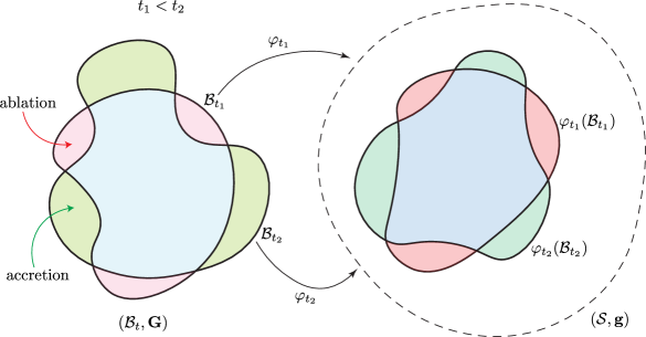
Figure 1: Motion of an accreting-ablating elastic body. The material manifold is a time-dependent Riemannian manifold $(\mathcal{B}_{t},\mathbf{G})$ whose metric is to be determined. The deformed body is embedded in the Euclidean ambient space $(\mathcal{S},\mathbf{g})$, where $\mathbf{g}$ is a time-independent background metric.

2.1 Riemannian geometry and kinematics of finite deformations

In this section we tersely review some basic concepts of Riemannian geometry that are used in the description of the kinematics of accreting-ablating bodies. A smooth $3$-manifold $\mathcal{B}$ is a topological space that locally looks like the three-dimensional Euclidean space $\mathbb{R}^{3}$. A coordinate chart $\{X^{A}\}:\mathcal{B}\to\mathbb{R}^{3}$ is a local diffeomorphism. The body in its reference configuration is identified with the $3$-manifold $\mathcal{B}$. The tangent space of $\mathcal{B}$ at a point $X\in\mathcal{B}$ is a three-dimensional linear space and is denoted by $T_{X}\mathcal{B}$. The three-dimensional Euclidean ambient space is denoted by $\mathcal{S}$. A local chart on $\mathcal{S}$ is denoted by $\{x^{a}\}$. Motion $\varphi_{t}:\mathcal{B}\to\mathcal{S}$ is a one-parameter family of smooth, invertible, and orientation preserving maps between the reference configuration and the ambient space (more precisely, motion is a curve $t\mapsto\varphi_{t}$ in the space of all configurations of $\mathcal{B}$). The derivative (tangent) map of $\varphi_{t}$ is denoted by $\mathbf{F}_{t}=T\varphi_{t}$, and is a two-point tensor, i.e., is a linear map between tangent spaces of two different manifolds, $\mathbf{F}(X,t):T_{X}\mathcal{B}\to T_{x}\mathcal{C}_{t}$, where $x=\varphi(X)$ and $\mathcal{C}_{t}=\varphi_{t}(\mathcal{B})$. In the continuum mechanics literature $\mathbf{F}$ is called deformation gradient. This term may be misleading as gradient is a metric-dependent operator while the tangent map is not. With respect to the local coordinate charts $\{X^{A}\}$ and $\{x^{a}\}$ for $\mathcal{B}$ and $\mathcal{S}$, respectively, deformation gradient has the following representation

$$\mathbf{F}=F^{a}{}_{A}\,\frac{\partial}{\partial x^{a}}\otimes dX^{A},\qquad F^{a}{}_{A}=\frac{\partial\varphi^{a}}{\partial X^{A}}\,.$$ (2.1)

The set of vectors $\big{\{}\frac{\partial}{\partial x^{a}}\big{\}}$ and co-vectors ($1$-forms) $\{dX^{A}\}$ are bases for the tangent space $T_{x}\mathcal{C}$ and co-tangent space $T^{*}_{X}\mathcal{B}$, respectively. A smooth vector field on $\mathcal{B}$ is a smooth assignment of vectors (elements of the tangent space) to points of $\mathcal{B}$. Thus, for a smooth vector field $\mathbf{W}$ on $\mathcal{B}$, $\mathbf{W}_{X}\in T_{X}\mathcal{B}$, $X\mapsto\mathbf{W}_{X}\in T_{X}\mathcal{B}$ varies smoothly. Push-forward of a vector field on $\mathcal{B}$ by the deformation mapping is a vector field in the ambient space and is defined as $\varphi_{*}\mathbf{W}=T\varphi\cdot\mathbf{W}\circ\varphi^{-1}$. Pull-back of a vector field $\mathbf{w}$ on $\mathcal{C}=\varphi(\mathcal{B})$ is a vector field on $\mathcal{B}$ and is defined as $\varphi^{*}\mathbf{w}=T(\varphi^{-1})\cdot\mathbf{w}\circ\varphi$. The push-forward and pull-back of vectors have the following coordinate representations: $(\varphi_{*}\mathbf{W})^{a}=F^{a}{}_{A}\,W^{A}$, and $(\varphi^{*}\mathbf{w})^{A}=F_{a}{}^{-A}\,w^{a}$.

A bilinear map $\mathbf{T}:T_{X}\mathcal{B}\times T_{X}\mathcal{B}\to\mathbb{R}$ is a $({}^{0}_{2})$-tensor at $X\in\mathcal{B}$. In a local coordinate chart $\{X^{A}\}$ for $\mathcal{B}$ and arbitrary vectors $\mathbf{U}$ and $\mathbf{W}$, one writes $\mathbf{T}(\mathbf{U},\mathbf{W})=T_{AB}\,U^{A}\,W^{B}$. Let us consider an inner product $\mathbf{G}_{X}$ on the tangent space $T_{X}\mathcal{B}$ that varies smoothly, i.e., if $\mathbf{U}$ and $\mathbf{W}$ are vector fields on $\mathcal{B}$, then $X\mapsto\mathbf{G}_{X}(\mathbf{U}_{X},\mathbf{W}_{X})$ is a smooth function. A positive-definite bilinear form $\mathbf{G}$ is called a metric. The inner product induced by the metric $\mathbf{G}_{X}$ is denoted by $\mathopen{\hbox{\set@color${\langle}$}\mkern 2.0mu\kern-3.49998pt\leavevmode\hbox{\set@color${\langle}$}}.,.\mathclose{\hbox{\set@color${\rangle}$}\mkern 2.0mu\kern-3.49998pt\leavevmode\hbox{\set@color${\rangle}$}}_{\mathbf{G}_{X}}$. The manifold $\mathcal{B}$ equipped with a smooth metric $\mathbf{G}$ is called a Riemannian manifold and is denoted as $(\mathcal{B},\mathbf{G})$. Distances in the ambient space are calculated using the background Euclidean metric $\mathbf{g}$. The Riemannian manifold $(\mathcal{S},\mathbf{g})$ is called the ambient space manifold. In elasticity, the reference configuration inherits a flat metric $\mathbf{G}_{0}$ from the ambient space and the material manifold $(\mathcal{B},\mathbf{G}_{0})$ is flat. In anelasticity the natural distances explicitly depend on the source of anelasticity and so does the material metric $\mathbf{G}$, which is non-flat, in general. For the two Riemannian manifolds $(\mathcal{B},\mathbf{G})$ and $(\mathcal{C},\mathbf{g})$, and the deformation mapping $\varphi:\mathcal{B}\to\mathcal{C}$, push-forward of the metric $\mathbf{G}$ is denoted by $\varphi_{*}\mathbf{G}$, which is a metric on $\mathcal{C}=\varphi(\mathcal{B})$, and is defined as

$$\mathopen{\hbox{\set@color${\langle}$}\mkern 2.0mu\kern-3.49998pt\leavevmode\hbox{\set@color${\langle}$}}\mathbf{u}_{x},\mathbf{w}_{x}\mathclose{\hbox{\set@color${\rangle}$}\mkern 2.0mu\kern-3.49998pt\leavevmode\hbox{\set@color${\rangle}$}}_{(\varphi*\mathbf{G})_{x}}=\mathopen{\hbox{\set@color${\langle}$}\mkern 2.0mu\kern-3.49998pt\leavevmode\hbox{\set@color${\langle}$}}(\varphi^{*}\mathbf{u})_{X},(\varphi^{*}\mathbf{w})_{X}\mathclose{\hbox{\set@color${\rangle}$}\mkern 2.0mu\kern-3.49998pt\leavevmode\hbox{\set@color${\rangle}$}}_{\mathbf{G}_{X}}\,,$$ (2.2)

where $x=\varphi(X)$. It has components $(\varphi_{*}\mathbf{G})_{ab}=F_{a}{}^{-A}\,F_{b}{}^{-B}\,G_{AB}$. Similarly, the pull-back of the metric $\mathbf{g}$ is denoted by $\varphi^{*}\mathbf{g}$ and is a metric in $\varphi^{-1}(\mathcal{C})=\mathcal{B}$ defined as

$$\mathopen{\hbox{\set@color${\langle}$}\mkern 2.0mu\kern-3.49998pt\leavevmode\hbox{\set@color${\langle}$}}\mathbf{U}_{X},\mathbf{W}_{X}\mathclose{\hbox{\set@color${\rangle}$}\mkern 2.0mu\kern-3.49998pt\leavevmode\hbox{\set@color${\rangle}$}}_{(\varphi^{*}\mathbf{g})_{X}}=\mathopen{\hbox{\set@color${\langle}$}\mkern 2.0mu\kern-3.49998pt\leavevmode\hbox{\set@color${\langle}$}}(\varphi_{*}\mathbf{U})_{x},(\varphi_{*}\mathbf{W})_{x}\mathclose{\hbox{\set@color${\rangle}$}\mkern 2.0mu\kern-3.49998pt\leavevmode\hbox{\set@color${\rangle}$}}_{\mathbf{g}_{x}}\,.$$ (2.3)

It has components, $(\varphi^{*}\mathbf{g})_{AB}=F^{a}{}_{A}\,F^{b}{}_{B}\,g_{ab}$. The two Riemannian manifolds $(\mathcal{B},\mathbf{G})$ and $(\mathcal{C},\mathbf{g})$ are called isometric if $\mathbf{G}=\varphi^{*}\mathbf{g}$, or equivalently, $\mathbf{g}=\varphi_{*}\mathbf{G}$. In this case, $\varphi$ is called an isometry.

The adjoint of deformation gradient $\mathbf{F}^{\star}(X,t):T^{*}_{x}\mathcal{C}_{t}\to T^{*}_{X}\mathcal{B}$ is defined such that

$$\langle\bm{\alpha},\mathbf{F}\mathbf{W}\rangle=\langle\mathbf{F}^{\star}\bm{\alpha},\mathbf{W}\rangle\,,\quad\forall\mathbf{W}\in T_{X}\mathcal{B}\,,~{}\bm{\alpha}\in T^{*}_{X}\mathcal{C}\,,$$ (2.4)

where $\langle.,.\rangle$ is the natural paring of $1$-forms and vectors, e.g., $\langle\bm{\alpha},\mathbf{w}\rangle=\alpha_{a}\,w^{a}$, and $T^{*}_{X}\mathcal{B}$ and $T^{*}_{x}\mathcal{C}_{t}$ are the co-tangent spaces of $\mathcal{B}$ at $X$ and $\mathcal{C}_{t}$ at $x$, respectively. $\mathbf{F}^{\star}$ has the following coordinate representation

$$\mathbf{F}^{\star}(X,t)=\frac{\partial\varphi^{a}(X,t)}{\partial X^{A}}\,dX^{A}\otimes\frac{\partial}{\partial x^{a}}\,.$$ (2.5)

The transpose of the deformation gradient $\mathbf{F}^{\mathsf{T}}(X,t):T_{x}\mathcal{C}_{t}\to T_{X}\mathcal{B}$ is defined such that

$$\mathopen{\hbox{\set@color${\langle}$}\mkern 2.0mu\kern-3.49998pt\leavevmode\hbox{\set@color${\langle}$}}\mathbf{F}\mathbf{U},\mathbf{w}\mathclose{\hbox{\set@color${\rangle}$}\mkern 2.0mu\kern-3.49998pt\leavevmode\hbox{\set@color${\rangle}$}}_{\mathbf{g}}=\mathopen{\hbox{\set@color${\langle}$}\mkern 2.0mu\kern-3.49998pt\leavevmode\hbox{\set@color${\langle}$}}\mathbf{U},\mathbf{F}^{\mathsf{T}}\mathbf{w}\mathclose{\hbox{\set@color${\rangle}$}\mkern 2.0mu\kern-3.49998pt\leavevmode\hbox{\set@color${\rangle}$}}_{\mathbf{G}}\,,\quad\forall\mathbf{U}\in T_{X}\mathcal{B}\,,~{}\mathbf{w}\in T_{X}\mathcal{C}\,.$$ (2.6)

It has the components $\big{(}F^{\mathsf{T}}\big{)}^{A}{}_{a}=G^{AB}F^{b}{}_{B}\,g_{ba}$, or $\mathbf{F}^{\mathsf{T}}=\mathbf{G}^{\sharp}\mathbf{F}^{\star}\mathbf{g}$.

The Jacobian of deformation $J(X,t)$ relates the undeformed and deformed volume elements as $dv\circ\varphi(X,t)=J(X,t)\,dV(X,t)$. It is defined as

$$J(X,t)=\sqrt{\frac{\det\mathbf{g}(\varphi(X,t))}{\det\mathbf{G}(X)}}\det\mathbf{F}(X,t)\,.$$ (2.8)

For incompressible materials, $J(X,t)=1$.

The material velocity is defined as $\mathbf{V}(X,t)=\frac{\partial\varphi(X,t)}{\partial t}\in T_{\varphi_{t}(X)}\mathcal{C}_{t}$. The spatial velocity is defined as $\mathbf{v}_{t}(x)=\mathbf{V}_{t}\circ\varphi_{t}^{-1}(x)\in T_{x}\mathcal{C}_{t}$, where $x=\varphi_{t}(X)$. The material acceleration is defined as $\mathbf{A}(X,t)=D^{\mathbf{g}}_{t}\mathbf{V}(X,t)=\nabla^{\mathbf{g}}_{\mathbf{V}(X,t)}\mathbf{V}(X,t)\in T_{\varphi_{t}(X)}\mathcal{C}_{t}$, where $D^{\mathbf{g}}_{t}$ is the covariant derivative along the curve $\varphi_{t}(X)$ in $\mathcal{C}_{t}$. In components, $A^{a}=\frac{\partial V^{a}}{\partial t}+\gamma^{a}{}_{bc}V^{b}V^{c}$. The spatial acceleration is defined as $\mathbf{a}_{t}(x)=\mathbf{A}_{t}\circ\varphi_{t}^{-1}(x)\in T_{x}\mathcal{C}_{t}$. It has components, $a^{a}=\frac{\partial v^{a}}{\partial t}+\frac{\partial v^{a}}{\partial x^{b}}v^{b}+\gamma^{a}{}_{bc}v^{b}v^{c}$. Equivalently, the spatial acceleration is the material time derivative of $\mathbf{v}$, i.e., $\mathbf{a}=\dot{\mathbf{v}}=\frac{\partial\mathbf{v}}{\partial t}+\nabla_{\mathbf{v}}^{\mathbf{g}}\mathbf{v}$.

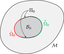
Figure 2: An initial body $\mathcal{B}_{0}$ in the material ambient space $\mathcal{M}$ and partitioning of its boundary into accretion, ablation, and inactive surfaces.

2.2 Kinematics of accreting-ablating bodies

Consider an initial stress-free body $\mathcal{B}_{0}$ that inherits the (flat) metric $\mathbf{G}_{0}$ from the Euclidean ambient space. The boundary of the initial body is partitioned as $\partial\mathcal{B}_{0}=\accentset{+}{\Omega}_{0}\sqcup\accentset{-}{\Omega}_{0}\sqcup\Pi_{0}$, where $\accentset{+}{\Omega}_{0}$, $\accentset{-}{\Omega}_{0}$, and $\Pi_{0}$ are the accretion, ablation, and inactive parts of the boundary, respectively, and $\sqcup$ denotes the disjoint union of sets (see Fig. 2). It should be noted that $\mathcal{B}_{0}$ is the initial body prior to the onset of accretion-ablation, $\accentset{+}{\Omega}_{0}$ represents the portion of $\partial\mathcal{B}_{0}$ where accretion is about to occur, and $\accentset{-}{\Omega}_{0}$ comprises of the points that are about to leave once the process starts at $t=0$. In other words, as soon as accretion-ablation begins, the body ceases to be the set $\mathcal{B}_{0}$; the points on $\accentset{-}{\Omega}_{0}$ leave and new points are attached onto $\accentset{+}{\Omega}_{0}$.

Let $\mathcal{M}\supset\mathcal{B}_{0}$ be a connected and orientable $3$-manifold with boundary embeddable in $\mathbb{R}^{3}$. This is called the material ambient space. The accretion-ablation process occurs in the time interval $t\in[0,T]$, where $T$ is the final time. Let us define a time of attachment map $\accentset{+}{\tau}:(\mathcal{M}\setminus\mathcal{B}_{0})\cup\accentset{+}{\Omega}_{0}\to[0,T]$ and a time of detachment map $\accentset{-}{\tau}:\accentset{-}{\mathcal{A}}_{T}\subset\mathcal{M}\to[0,T]$, where $\accentset{-}{\mathcal{A}}_{T}$ is the subset of $\mathcal{M}$ that is ablated in the time interval $[0,T]$. Note that $\accentset{+}{\tau}^{-1}(0)=\accentset{+}{\Omega}_{0}$, and $\accentset{-}{\tau}^{-1}(0)=\accentset{-}{\Omega}_{0}$. Let us define the reference configuration at time $t$ as

$$\mathcal{B}_{t}:=\left(\mathcal{B}_{0}\cup\accentset{+}{\tau}^{-1}(0,t]\right)\setminus\accentset{-}{\tau}^{-1}[0,t)\,,\quad\forall t\in[0,T]\,,$$ (2.9)

which is constructed by removing all the points that have been ablated out before time $t$ from the union of $\mathcal{B}_{0}$ and the points accreted onto $\mathcal{B}_{0}$ up to time $t$. It is assumed that the differentials d$\accentset{+}{\tau}$ and d$\accentset{-}{\tau}$ never vanish. Let us introduce the level sets

$$\accentset{+}{\Omega}_{t}=\accentset{+}{\tau}^{-1}(t)\,,\qquad\accentset{-}{\Omega}_{t}=\accentset{-}{\tau}^{-1}(t)\,,\quad t\in[0,T]\,,$$ (2.10)

and define

$$\accentset{+}{\mathcal{A}}_{t}=\displaystyle\bigcup\limits_{\accentset{+}{\tau}\in[0,t]}\accentset{+}{\Omega}_{\accentset{+}{\tau}}\,,\qquad\accentset{-}{\mathcal{A}}_{t}=\displaystyle\bigcup\limits_{\accentset{-}{\tau}\in[0,t]}\accentset{-}{\Omega}_{\accentset{-}{\tau}}\,,\quad t\in[0,T]\,.$$ (2.11)

It is assumed that $\accentset{+}{\Omega}_{t}$ and $\accentset{-}{\Omega}_{t}$ are $2$-manifolds. It is also assumed that all $\accentset{+}{\Omega}_{t}$’s are diffeomorphic to $\accentset{+}{\Omega}_{0}$ and all $\accentset{-}{\Omega}_{t}$’s are diffeomorphic to $\accentset{-}{\Omega}_{0}$. Since accretion and ablation cannot take place at a given point and at the same time, it is required that

$$\accentset{+}{\Omega}_{t}\cap\accentset{-}{\Omega}_{t}=\emptyset\,,\quad\forall\,t\in[0,T]\,.$$ (2.12)

It should be emphasized that the intersection $\accentset{+}{\mathcal{A}}_{t}\cap\accentset{-}{\mathcal{A}}_{t}$ may be nonempty, see Fig. 3. Note that $\mathcal{M}=(\accentset{+}{\mathcal{A}}_{T}\setminus\accentset{+}{\Omega}_{0})\cup\mathcal{B}_{0}$, and

$$\mathcal{B}_{t}=\left(\mathcal{B}_{0}\cup(\accentset{+}{\mathcal{A}}_{t}\setminus\accentset{+}{\Omega}_{0})\right)\setminus(\accentset{-}{\mathcal{A}}_{t}\setminus\accentset{-}{\Omega}_{t})\,,\quad t\in[0,T]\,.$$ (2.13)

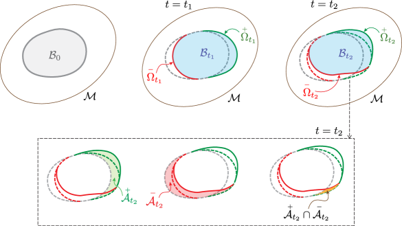
Figure 3: The material manifold is shown at times $t_{1}$ and $t_{2}$ where $t_{1}<t_{2}$. The accretion boundaries are shown in green and the ablation boundaries are shown in red. It should be noted that the set of all those points that have been ablated until time $t_{2}$ may include points other than those in the initial body.

The deformation mapping $\varphi_{t}:\mathcal{B}_{t}\to\mathcal{C}_{t}$ is assumed to be a $C^{1}$ homeomorphism for each $t$, where $\mathcal{C}_{t}=\varphi_{t}(\mathcal{B}_{t})$ is the current configuration of the accreting-ablating body. The deformed level sets are defined as $\accentset{+}{\omega}_{t}=\varphi_{t}(\accentset{+}{\Omega}_{t})$, and $\accentset{-}{\omega}_{t}=\varphi_{t}(\accentset{-}{\Omega}_{t})$. We denote the non-active portion of the boundary by $\Pi_{t}=\partial\mathcal{B}_{t}\setminus(\accentset{+}{\Omega}_{t}\cup\accentset{-}{\Omega}_{t})$ in the reference configuration and $\pi_{t}=\varphi_{t}(\Pi_{t})$ in the deformed configuration, so that

$$\partial\varphi_{t}(\mathcal{B}_{t})=\varphi_{t}(\accentset{+}{\Omega}_{t}\cup\accentset{-}{\Omega}_{t}\cup\Pi_{t})=\accentset{+}{\omega}_{t}\cup\accentset{-}{\omega}_{t}\cup\pi_{t}\,.$$ (2.14)

For $X\in\mathcal{M}$ and $\accentset{+}{\tau}(X)\leq t<\accentset{-}{\tau}(X)$, denote $\varphi(X,t)=\varphi_{t}(X)$. Let us define the following two time-independent maps

$$\accentset{+}{\varphi}(X):=\varphi(X,\accentset{+}{\tau}(X))\,,\qquad\accentset{-}{\varphi}(X):=\varphi(X,\accentset{-}{\tau}(X))\,,$$ (2.15)

where $\accentset{+}{\varphi}$ is defined on $\accentset{+}{\mathcal{A}}_{T}$ and $\accentset{-}{\varphi}$ is defined on $\accentset{-}{\mathcal{A}}_{T}$. Note that for $t\in[0,T]$

$$\accentset{+}{\varphi}(\accentset{+}{\mathcal{A}}_{t})=\displaystyle\bigcup\limits_{{\accentset{+}{\tau}}\in[0,t]}\accentset{+}{\omega}_{\accentset{+}{\tau}}\,,\qquad\accentset{-}{\varphi}(\accentset{-}{\mathcal{A}}_{t})=\displaystyle\bigcup\limits_{{\accentset{-}{\tau}}\in[0,t]}\accentset{-}{\omega}_{\accentset{-}{\tau}}\,.$$ (2.16)

It should be noted that $\accentset{+}{\varphi}$ and $\accentset{-}{\varphi}$ need not be injective. Next, we define the following two-point tensors

$$\accentset{+}{\mathbf{F}}(X):=\mathbf{F}(X,\accentset{+}{\tau}(X))\,,\qquad\accentset{-}{\mathbf{F}}(X):=\mathbf{F}(X,\accentset{-}{\tau}(X))\,,$$ (2.17)

and call them the accretion and ablation frozen deformation gradients, respectively. The derivative maps $T\accentset{+}{\varphi}$ and $T\accentset{-}{\varphi}$ are neither injective nor invertible, in general. They are related to $\accentset{+}{\mathbf{F}}$ and $\accentset{-}{\mathbf{F}}$ as

$$(T\accentset{+}{\varphi})^{i}{}_{J} =\frac{\partial\varphi^{i}(X,\accentset{+}{\tau}(X))}{\partial X^{J}}=F^{i}{}_{J}(X,\accentset{+}{\tau}(X))+V^{i}(X,\accentset{+}{\tau}(X))\frac{\partial\accentset{+}{\tau}(X)}{\partial X^{J}}=\accentset{+}{F}^{i}{}_{J}+\accentset{+}{V}^{i}\frac{\partial\accentset{+}{\tau}}{\partial X^{J}}\,,$$ (2.18)

$$(T\accentset{-}{\varphi})^{i}{}_{J} =\accentset{-}{F}^{i}{}_{J}+\accentset{-}{V}^{i}\frac{\partial{\accentset{-}{\tau}}}{\partial X^{J}}\,,$$

where $\accentset{+}{\mathbf{V}}(X):=\mathbf{V}_{\accentset{+}{\tau}(X)}(X)$, and $\accentset{-}{\mathbf{V}}(X):=\mathbf{V}_{\accentset{-}{\tau}(X)}(X)$. The coordinate-free forms of (2.18) read

$$T\accentset{+}{\varphi}=\accentset{+}{\mathbf{F}}+\accentset{+}{\mathbf{V}}\otimes\text{d}\accentset{+}{\tau}\,,\qquad T\accentset{-}{\varphi}=\accentset{-}{\mathbf{F}}+\accentset{-}{\mathbf{V}}\otimes\text{d}{\accentset{-}{\tau}}\,.$$ (2.19)

For $t\in[0,T]$, on each layer, one has $\accentset{+}{\mathbf{F}}|_{T\accentset{+}{\Omega}_{t}}=T\accentset{+}{\varphi}|_{T\accentset{+}{\Omega}_{t}}=\mathbf{F}_{t}|_{T\accentset{+}{\Omega}_{t}}$, and $\accentset{-}{\mathbf{F}}|_{T\accentset{-}{\Omega}_{t}}=T\accentset{+}{\varphi}|_{T\accentset{-}{\Omega}_{t}}=\mathbf{F}_{t}|_{T\accentset{-}{\Omega}_{t}}$.

2.3 The Growth velocity and the material metric

The material metric of an accreting-ablating body at a given material point depends on the state of stress of the accreting particles, the growth velocity, and the state of deformation of the body at the time of attachment of the new material point. One can define an accretion tensor via the frozen deformation gradient and a material growth velocity. Material metric is then defined to be the pull-back of the ambient space metric by the accretion tensor [Sozio and Yavari, 2017]. The time dependence of an accreting body can be modeled as a material motion in the material ambient space. It turns out that given a time of attachment map such material motions are not unique; instead one can define an equivalence class of material motions. Using any member of the equivalence class results in the same material metric. In the presence of ablation one has two material motions. Again, these are not unique. For calculating the material metric only the accretion material motion is needed as we are not concerned with the material metric of a particle after it has left the body. In the following we briefly review the construction of the material metric.

In an accreting-ablating body, what is given is the rate at which material points are added to the body on the accretion boundary and the rate at which material points are removed from the ablation boundary. These two vector fields may be unknown fields in the presence of phase change, for example. In this paper, we assume that they are given. It should be emphasized that the material analogues of the accretion and ablation velocities are not defined uniquely.

Recall that we have assumed that for $t\in(0,T]$, $\accentset{+}{\Omega}_{t}$ is diffeomorphic to $\accentset{+}{\Omega}_{0}$ and $\accentset{-}{\Omega}_{t}$ is diffeomorphic to $\accentset{-}{\Omega}_{0}$. This guarantees the existence of $1$-parameter families of diffeomorphisms $\accentset{+}{\Phi}:\accentset{+}{\Omega}_{0}\times[0,T]\to\mathcal{M}$, and $\accentset{-}{\Phi}:\accentset{-}{\Omega}_{0}\times[0,T]\to\mathcal{M}$, such that $\accentset{+}{\Phi}(\accentset{+}{\Omega}_{0},t)=\accentset{+}{\Omega}_{t}$, and $\accentset{-}{\Phi}(\accentset{-}{\Omega}_{0},t)=\accentset{-}{\Omega}_{t},~{}\forall t\in[0,T]$. However, these diffeomorphisms are not unique. Let us fix two diffeomorphisms $\accentset{+}{\Phi}$ and $\accentset{-}{\Phi}$. For $X\in\accentset{+}{\mathcal{A}}_{T}$, there is a unique $\accentset{+}{X_{0}}\in\accentset{+}{\Omega}_{0}$ such that $\accentset{+}{\Phi}(\accentset{+}{X_{0}},\accentset{+}{\tau}(X))=\accentset{+}{\Phi}_{\accentset{+}{\tau}(X)}(\accentset{+}{X_{0}})=X$. Similarly, for $X\in\accentset{-}{\mathcal{A}}_{T}$ there is a unique $\accentset{-}{X_{0}}\in\accentset{-}{\Omega}_{0}$ such that $\accentset{-}{\Phi}(\accentset{-}{X_{0}},{\accentset{-}{\tau}}(X))=\accentset{-}{\Phi}_{{\accentset{-}{\tau}}(X)}(\accentset{-}{X_{0}})=X$. The maps $\accentset{+}{\Phi}$ and $\accentset{-}{\Phi}$ define a pair of motions of layers in the material manifold, with which we associate the following velocities

$$\accentset{+}{\mathbf{U}}(\accentset{+}{X_{0}},t)=\frac{\partial}{\partial t}\accentset{+}{\Phi}(\accentset{+}{X_{0}},t)\,,\qquad\accentset{-}{\mathbf{U}}(\accentset{-}{X_{0}},t)=\frac{\partial}{\partial t}\accentset{-}{\Phi}(\accentset{-}{X_{0}},t)\,.$$ (2.20)

Differentiating the relations $\accentset{+}{\tau}(\accentset{+}{\Phi}(\accentset{+}{X_{0}},t))=t$, and ${\accentset{-}{\tau}}(\accentset{-}{\Phi}(\accentset{-}{X_{0}},t))=t$ with respect to time, one obtains the following constraints

$$\big{\langle}\text{d}\accentset{+}{\tau}(X),\accentset{+}{\mathbf{U}}(\accentset{+}{X_{0}},t)\big{\rangle}=1\,,\qquad\big{\langle}\text{d}{\accentset{-}{\tau}}(X),\accentset{-}{\mathbf{U}}(\accentset{-}{X_{0}},t)\big{\rangle}=1\,,$$ (2.21)

where $\accentset{+}{\Phi}(\accentset{+}{X_{0}},t)=X=\accentset{-}{\Phi}(\accentset{-}{X_{0}},t)$. It should be emphasized that for a given pair of time of attachment and time of detachment maps, material motion is not uniquely defined; there are infinitely many material motions corresponding to a given pair $(\accentset{+}{\tau},\accentset{-}{\tau})$. These equivalent material motions satisfy the constraint (2.21)₁ [Sozio and Yavari, 2019] and correspond to isometric material metrics.

One can define a material motion $(\accentset{+}{\Phi}_{t},\accentset{-}{\Phi}_{t})$ using foliation charts $(\Xi^{1},\Xi^{2},\accentset{+}{\tau})$ on $\accentset{+}{\mathcal{A}}_{T}$, and $(\Theta^{1},\Theta^{2},{\accentset{-}{\tau}})$ on $\accentset{-}{\mathcal{A}}_{T}$, where $(\Xi^{1},\Xi^{2})$ and $(\Theta^{1},\Theta^{2})$ are the in-layer coordinates on $\accentset{+}{\Omega}_{\accentset{+}{\tau}}$ and $\accentset{-}{\Omega}_{\accentset{-}{\tau}}$, respectively, while $\accentset{+}{\tau}$ and ${\accentset{-}{\tau}}$ are globally defined on $\accentset{+}{\mathcal{A}}_{T}$ and $\accentset{-}{\mathcal{A}}_{T}$, respectively. The material motion preserves the in-layer coordinates $(\Xi^{1},\Xi^{2})$ and $(\Theta^{1},\Theta^{2})$. This means that if $X_{0}\in\accentset{+}{\Omega}_{0}$ has coordinates $(\Xi^{1},\Xi^{2},0)$, then $\accentset{+}{\Phi}_{t}$ maps it to the point $X_{t}$ with coordinates $(\Xi^{1},\Xi^{2},t)$. Similarly, if $X_{0}\in\accentset{-}{\Omega}_{0}$ has coordinates $(\Theta^{1},\Theta^{2})$, then $\accentset{-}{\Phi}_{t}$ maps it to the point $X_{t}$ with coordinates $(\Theta^{1},\Theta^{2},t)$. Trajectories of the material motion are the curves with constant layer coordinates, i.e., $\accentset{+}{\tau}$-lines and $\accentset{-}{\tau}$-lines. The growth and ablation velocities corresponding to $\accentset{+}{\Phi}_{t}$ and $\accentset{-}{\Phi}_{t}$, respectively, are defined as

$$\accentset{+}{\mathbf{U}}=\left.\frac{\partial}{\partial\accentset{+}{\tau}}\right\rvert_{\Xi^{1},\Xi^{2}}\,,\qquad\accentset{-}{\mathbf{U}}=\left.\frac{\partial}{\partial\accentset{-}{\tau}}\right\rvert_{\Theta^{1},\Theta^{2}}\,.$$ (2.22)

Notice that $\left\langle\text{d}\accentset{+}{\tau},\frac{\partial}{\partial\accentset{+}{\tau}}\right\rangle=1$, and $\left\langle\text{d}{\accentset{-}{\tau}},\frac{\partial}{\partial{\accentset{-}{\tau}}}\right\rangle=1$.

Let us next calculate the total velocities of $\accentset{+}{\omega}_{t}$ and $\accentset{-}{\omega}_{t}$. The map $\accentset{+}{\varphi}\circ\accentset{+}{\Phi}:\accentset{+}{\Omega}_{0}\times[0,T]\to\mathcal{S}$ tracks the deformed accretion surface $\accentset{+}{\omega}_{t}$, and $\accentset{-}{\varphi}\circ\accentset{-}{\Phi}:\accentset{-}{\Omega}_{0}\times[0,T]\to\mathcal{S}$ tracks the deformed ablation surface $\accentset{-}{\omega}_{t}$. The total velocities are calculated as

$$\accentset{+}{\mathbf{W}}(X) =\frac{\text{d}}{\text{d}t}\accentset{+}{\varphi}\big{(}\accentset{+}{\Phi}(\accentset{+}{X_{0}},t)\big{)}=[\accentset{+}{\mathbf{F}}(X)+\accentset{+}{\mathbf{V}}(X)\otimes\text{d}\accentset{+}{\tau}(X)]\accentset{+}{\mathbf{U}}(\accentset{+}{X_{0}},t)=\accentset{+}{\mathbf{F}}(X)\accentset{+}{\mathbf{U}}(\accentset{+}{X_{0}},t)+\accentset{+}{\mathbf{V}}(X)\,,$$ (2.23)

$$\accentset{-}{\mathbf{W}}(X) =\frac{\text{d}}{\text{d}t}\accentset{-}{\varphi}\big{(}\accentset{-}{\Phi}(\accentset{-}{X_{0}},t)\big{)}=[\accentset{-}{\mathbf{F}}(X)+\accentset{-}{\mathbf{V}}(X)\otimes\text{d}{\accentset{-}{\tau}}(X)]\accentset{-}{\mathbf{U}}(\accentset{-}{X_{0}},t)=\accentset{-}{\mathbf{F}}(X)\accentset{-}{\mathbf{U}}(\accentset{-}{X_{0}},t)+\accentset{-}{\mathbf{V}}(X)\,.$$

The spatial velocities are defined as $\accentset{+}{\mathbf{w}}\circ\varphi=\accentset{+}{\mathbf{W}}$ and $\accentset{-}{\mathbf{w}}\circ\varphi=\accentset{-}{\mathbf{W}}$. Let $\accentset{+}{\mathbf{u}}_{t}$ be a vector field describing the velocity at which material is being added onto $\accentset{+}{\omega}_{t}$, i.e., $-\accentset{+}{\mathbf{u}}_{t}$ is its relative velocity with respect to $\accentset{+}{\omega}_{t}$ just before attachment, and let $-\accentset{-}{\mathbf{u}}_{t}$ be a vector field describing the velocity at which material is being removed from $\accentset{-}{\omega}_{t}$, i.e., $\accentset{-}{\mathbf{u}}_{t}$ is its relative velocity with respect to $\accentset{-}{\omega}_{t}$ just after detachment. If $\mathbf{n}_{t}$ denotes the unit normal to $\varphi_{t}(\partial\mathcal{B}_{t})$, then we must have $(-\accentset{+}{\mathbf{u}}_{t})\cdot\mathbf{n}_{t}<0$ for accretion, i.e., $\accentset{+}{\mathbf{u}}_{t}\cdot\mathbf{n}_{t}>0$, as the material would be moving towards the body. Similarly, in the case of ablation we need $\accentset{-}{\mathbf{u}}_{t}\cdot\mathbf{n}_{t}>0$ as the material removed would be moving away from the body.

For $X\in\mathcal{M}$, let us define the following time-independent tensor field

$$\mathbf{Q}(X)=\accentset{+}{\mathbf{F}}(X)+\Big{[}\accentset{+}{\mathbf{u}}_{\accentset{+}{\tau}(X)}\big{(}\accentset{+}{\varphi}(X)\big{)}-\accentset{+}{\mathbf{F}}(X)\accentset{+}{\mathbf{U}}\big{(}\accentset{+}{\Phi}_{\accentset{+}{\tau}(X)}^{-1}(X),\accentset{+}{\tau}(X)\big{)}\Big{]}\otimes\text{d}\accentset{+}{\tau}(X)\,,$$ (2.24)

where $\accentset{+}{\Phi}_{\accentset{+}{\tau}(X)}^{-1}(X)$ can be understood as the pull back of $X\in\mathcal{M}$ to $\accentset{+}{\Omega}_{0}$ along the trajectory induced by $\accentset{+}{\Phi}$. $\mathbf{Q}$ is called the accretion tensor [Sozio and Yavari, 2019]. Note that $\mathbf{Q}\big{(}\accentset{+}{\Phi}(\accentset{+}{X_{0}},t)\big{)}\accentset{+}{\mathbf{U}}\big{(}\accentset{+}{X_{0}},t\big{)}=\accentset{+}{\mathbf{u}}\big{(}(\accentset{+}{\varphi}\circ\accentset{+}{\Phi})(\accentset{+}{X_{0}},t),t\big{)}$, $\forall~{}\accentset{+}{X_{0}}\in\accentset{+}{\Omega}_{0}$. Let $\mathbf{g}$ be the metric of the Euclidean ambient space $\mathcal{S}$. Assuming that the new material points are stress-free at their time of attachment the material metric on $\accentset{+}{\mathcal{A}}_{T}$ is defined to be the pull-back of $\mathbf{g}$ using $\mathbf{Q}$, i.e.,

$$\mathbf{G}(X)=\mathbf{Q}^{\star}(X)\,\mathbf{g}\big{(}\accentset{+}{\varphi}(X)\big{)}\mathbf{Q}(X)\,,$$ (2.25)

or in components, $G_{IJ}(X)=Q^{I}{}_{J}(X)\,g_{ij}(\accentset{+}{\varphi}(X))\,Q^{j}{}_{J}(X)$. Therefore, the material metric is written as

$$\mathbf{G}(X)=\begin{cases}\mathbf{G}_{0}(X)&\text{for }X\in\mathcal{B}_{0}\,,\\ \mathbf{Q}^{\star}(X)\,\mathbf{g}\big{(}\accentset{+}{\varphi}(X)\big{)}\,\mathbf{Q}(X)&\text{for }X\in\accentset{+}{\mathcal{A}}_{T}\,.\end{cases}$$ (2.26)

The natural distances in the accreting-ablating body are measured using the material metric $\mathbf{G}$. Note that, for the layers that are joining the body, the material metric depends on the state of deformation of the body at the time of attachment. However, we are not interested in the state of deformation and stress of those layers that have already left the body. The material metric of those points after leaving the body has no effect on the rest of the body and does not appear in our accretion-ablation theory.

Remark 2.1.

The map $\accentset{+}{\tau}$ partitions the accreted manifold $(\accentset{+}{\mathcal{A}}_{T},\mathbf{G})$ into a collection of submanifolds $\big{\{}(\accentset{+}{\Omega}_{\accentset{+}{\tau}},\tilde{\mathbf{G}}_{\accentset{+}{\tau}}):\accentset{+}{\tau}\in[0,T]\big{\}}$. Similarly, ${\accentset{-}{\tau}}$ partitions the ablated manifold $(\accentset{-}{\mathcal{A}}_{T},\mathbf{G})$ into another collection of submanifolds $\big{\{}(\accentset{+}{\Omega}_{\accentset{-}{\tau}},\tilde{\mathbf{G}}_{\accentset{-}{\tau}}):{\accentset{-}{\tau}}\in[0,T]\big{\}}$. Here, $\tilde{\mathbf{G}}_{\accentset{+}{\tau}}$ and $\tilde{\mathbf{G}}_{\accentset{-}{\tau}}$ are the first fundamental forms inherited from $\mathbf{G}$ by $\accentset{+}{\Omega}_{\accentset{+}{\tau}}$ and $\accentset{-}{\Omega}_{\accentset{-}{\tau}}$, respectively. Let $\accentset{+}{\mathbf{N}}_{\accentset{+}{\tau}}$ and $\accentset{-}{\mathbf{N}}_{\accentset{-}{\tau}}$ be the unit normals to $\accentset{+}{\Omega}_{\accentset{+}{\tau}}$ and $\accentset{-}{\Omega}_{\accentset{-}{\tau}}$, respectively, where orthonormality is with respect to the metric $\mathbf{G}$. Let $\accentset{+}{\mathbf{n}}_{\accentset{+}{\tau}}$ and $\accentset{-}{\mathbf{n}}_{\accentset{-}{\tau}}$ be the unit normals to $\accentset{+}{\omega}_{\accentset{+}{\tau}}$ and $\accentset{-}{\omega}_{\accentset{-}{\tau}}$, respectively (here orthonormality is with respect to the ambient metric $\mathbf{g}$). Let us decompose the accretion and ablation velocities as

$$\accentset{+}{\mathbf{U}}=\accentset{+}{\mathbf{U}}^{\parallel}+\accentset{+}{U}^{\accentset{+}{N}}\,\accentset{+}{\mathbf{N}}\,,\qquad\accentset{-}{\mathbf{U}}=\accentset{-}{\mathbf{U}}^{\parallel}+\accentset{-}{U}^{\accentset{-}{N}}\,\accentset{-}{\mathbf{N}}\,,$$ (2.27)

in the material manifold and

$$\accentset{+}{\mathbf{u}}=\accentset{+}{\mathbf{u}}^{\parallel}+\accentset{+}{u}^{\accentset{+}{n}}\,\accentset{+}{\mathbf{n}}\,,\qquad\accentset{-}{\mathbf{u}}=\accentset{-}{\mathbf{u}}^{\parallel}+\accentset{-}{u}^{\accentset{-}{n}}\,\accentset{-}{\mathbf{n}}\,,$$ (2.28)

in the deformed configuration, where we have $\accentset{+}{u}^{\accentset{+}{n}},\,\accentset{-}{u}^{\accentset{-}{n}}>0$. Note that, if $\mathbf{Y}$ is tangent to $\accentset{+}{\Omega}$, then $\mathbf{Q}\mathbf{Y}$ is tangent to $\accentset{+}{\omega}$. Notice that $\mathopen{\hbox{\set@color${\langle}$}\mkern 2.0mu\kern-3.49998pt\leavevmode\hbox{\set@color${\langle}$}}\mathbf{Y},\mathbf{Q}^{-1}\accentset{+}{\mathbf{n}}\mathclose{\hbox{\set@color${\rangle}$}\mkern 2.0mu\kern-3.49998pt\leavevmode\hbox{\set@color${\rangle}$}}_{\mathbf{G}}=\mathopen{\hbox{\set@color${\langle}$}\mkern 2.0mu\kern-3.49998pt\leavevmode\hbox{\set@color${\langle}$}}\mathbf{Q}\mathbf{Y},\accentset{+}{\mathbf{n}}\mathclose{\hbox{\set@color${\rangle}$}\mkern 2.0mu\kern-3.49998pt\leavevmode\hbox{\set@color${\rangle}$}}_{\mathbf{g}}=0$, and $\mathopen{\hbox{\set@color${\langle}$}\mkern 2.0mu\kern-3.49998pt\leavevmode\hbox{\set@color${\langle}$}}\mathbf{Q}^{-1}\accentset{+}{\mathbf{n}},\mathbf{Q}^{-1}\accentset{+}{\mathbf{n}}\mathclose{\hbox{\set@color${\rangle}$}\mkern 2.0mu\kern-3.49998pt\leavevmode\hbox{\set@color${\rangle}$}}_{\mathbf{G}}=\mathopen{\hbox{\set@color${\langle}$}\mkern 2.0mu\kern-3.49998pt\leavevmode\hbox{\set@color${\langle}$}}\accentset{+}{\mathbf{n}},\accentset{+}{\mathbf{n}}\mathclose{\hbox{\set@color${\rangle}$}\mkern 2.0mu\kern-3.49998pt\leavevmode\hbox{\set@color${\rangle}$}}_{\mathbf{g}}=1$. Thus, it can be deduced that $\mathbf{Q}\accentset{+}{\mathbf{U}}^{\parallel}=\accentset{+}{\mathbf{u}}^{\parallel}$, $\mathbf{Q}\accentset{+}{\mathbf{N}}=\accentset{+}{\mathbf{n}}$, and hence $\accentset{+}{U}^{\accentset{+}{N}}=\accentset{+}{u}^{\accentset{+}{n}}\circ\varphi$.

2.4 Stress, strain, and constitutive equations

Strain.

A few different but related measures of strain are usually used in nonlinear elasticity and anelasticity [Marsden and Hughes, 1983, Ogden, 1984, Goriely, 2017, Yavari and Sozio, 2023]. The right Cauchy-Green strain is defined as $\mathbf{C}^{\flat}=\varphi^{*}\mathbf{g}=\mathbf{F}^{\star}\mathbf{g}\mathbf{F}$, which is the pulled-back of the spatial metric to the reference configuration. Here, $\flat:T_{x}\mathcal{C}\to T^{*}_{x}\mathcal{C}$ is the flat operator that maps a vector to its corresponding co-vector ($1$-form): $\mathbf{w}=w^{a}\frac{\partial}{\partial x^{a}}\mapsto\mathbf{w}^{\flat}=g_{ab}w^{b}\,dx^{a}$. In components, $C_{AB}=F^{a}{}_{A}\,g_{ab}F^{b}{}_{B}$. The familiar definition of the right Cauchy-Green stain is $\mathbf{C}=\mathbf{F}^{\mathsf{T}}\mathbf{F}:T_{X}\mathcal{B}\to\mathcal{B}$, which has components $C^{A}{}_{B}=G^{AM}C_{MB}=(G^{AM}F^{a}{}_{M}\,g_{ab})F^{b}{}_{B}=\big{(}F^{\mathsf{T}}\big{)}^{A}{}_{b}\,F^{b}{}_{B}$. The spatial analogue of the right Cauchy-Green strain is defined as $\mathbf{c}^{\flat}=\varphi_{*}\mathbf{G}=\mathbf{F}^{-\star}\mathbf{G}\mathbf{F}^{-1}$. The left Cauchy-Green strain is defined as $\mathbf{B}^{\sharp}=\varphi^{*}\mathbf{g}^{\sharp}$, where $\sharp:T^{*}_{x}\mathcal{C}\to T_{x}\mathcal{C}$ is the sharp operator that maps a co-vector ($1$-form) to its corresponding vector: $\bm{\omega}=\omega_{a}\,dx^{a}\mapsto\bm{\omega}^{\sharp}=g^{ab}\omega_{b}\,\frac{\partial}{\partial x^{a}}$. The left Cauchy-Green strain has components $B^{AB}=F^{-A}{}_{a}\,F^{-B}{}_{b}\,g^{ab}$, where $g^{ab}$ are components of the inverse spatial metric such that $g^{ac}g_{cb}=\delta^{a}_{b}$. The spatial analogue of $\mathbf{B}^{\sharp}$ is defined as $\mathbf{b}^{\sharp}=\varphi_{*}\mathbf{G}^{\sharp}=\mathbf{F}\mathbf{G}^{\sharp}\mathbf{F}^{\star}$, which has components $b^{ab}=F^{a}{}_{A}F^{b}{}_{B}\,G^{AB}$. The tensor $\mathbf{b}:T_{x}\mathcal{C}\to T_{x}\mathcal{C}$ is defined as $\mathbf{b}=\mathbf{b}^{\sharp}\mathbf{g}$. Similarly, $\mathbf{c}=\mathbf{g}^{\sharp}\mathbf{c}^{\flat}$. Notice that $\mathbf{c}\mathbf{b}=\mathbf{g}^{\sharp}\mathbf{c}^{\flat}\mathbf{b}^{\sharp}\mathbf{g}=\mathbf{g}^{\sharp}\mathbf{F}^{-\star}\mathbf{G}\mathbf{F}^{-1}\mathbf{F}\mathbf{G}^{\sharp}\mathbf{F}^{\star}\mathbf{g}=\mathbf{g}^{\sharp}\mathbf{F}^{-\star}\mathbf{G}\mathbf{G}^{\sharp}\mathbf{F}^{\star}\mathbf{g}=\mathbf{g}^{\sharp}\mathbf{F}^{-\star}\mathbf{F}^{\star}\mathbf{g}=\mathbf{g}^{\sharp}\mathbf{g}=\mathrm{id}_{\mathcal{S}}$, and hence $\mathbf{b}=\mathbf{c}^{-1}$. Similarly, $\mathbf{B}=\mathbf{C}^{-1}$.

Stress.

For a hyper-elastic solid there exists an energy function $W=W(X,\mathbf{F},\mathbf{G},\mathbf{g})$. Material-frame-indifference (objectivity) implies that $W=\hat{W}(X,\mathbf{C}^{\flat},\mathbf{G})$. The Cauchy $\bm{\sigma}$, the first Piola-Kirchhoff $\mathbf{P}$, and the second Piola-Kirchhoff $\mathbf{S}$ stress tensors are related to the energy function as

$$\mathbf{P}=\mathbf{g}^{\sharp}\frac{\partial W}{\partial\mathbf{F}}\,,\qquad\bm{\sigma}=\frac{2}{J}\frac{\partial W}{\partial\mathbf{g}}\,,\qquad\mathbf{S}=2\frac{\partial W}{\partial\mathbf{C}^{\flat}}\,.$$ (2.29)

They are also related as $\mathbf{S}=\mathbf{F}^{-1}\mathbf{P}$, and $\mathbf{P}=J\bm{\sigma}\mathbf{F}^{-\star}$. Let us consider a surface element $dA$ in the reference configuration with unit normal vector $\mathbf{N}$. This surface element is mapped to its deformed surface element $da$ with unit normal $\mathbf{n}$. Traction $\mathbf{t}$ is related to the Cauchy stress as $\mathbf{t}=\bm{\sigma}\cdot\mathbf{n}=\mathopen{\hbox{\set@color${\langle}$}\mkern 2.0mu\kern-3.49998pt\leavevmode\hbox{\set@color${\langle}$}}\bm{\sigma},\mathbf{n}\mathclose{\hbox{\set@color${\rangle}$}\mkern 2.0mu\kern-3.49998pt\leavevmode\hbox{\set@color${\rangle}$}}_{\mathbf{g}}$. In components, $t^{a}=\sigma^{ab}g_{bc}\,n^{c}$. The force acting on the deformed area element is $\mathbf{f}=\mathbf{t}da$. From the Piola identity $\mathbf{n}^{\flat}da=J\mathbf{F}^{-\star}\mathbf{N}^{\flat}dA$, or in components, $n_{a}da=J\,F^{-A}{}_{a}N_{A}dA$—Nanson’s formula. Thus, $\mathbf{f}=\mathbf{t}_{0}dA=\mathbf{P}\cdot\mathbf{N}dA$.

Material Symmetry.

For an elastic body the material symmetry group $\mathcal{G}_{X}$ at $X\in\mathcal{B}$ with respect to the reference configuration $(\mathcal{B},\mathbf{G})$ is defined as

$$W(X,\mathbf{K}^{*}\mathbf{F},\mathbf{K}^{*}\mathbf{G},\mathbf{g})=W(X,\mathbf{F}\mathbf{K},\mathbf{G},\mathbf{g})=W(X,\mathbf{F},\mathbf{G},\mathbf{g})\,,\qquad\forall\,\,\mathbf{K}\in\mathcal{G}_{X}\leqslant\mathrm{Orth}(\mathbf{G})\,,$$ (2.30)

for any deformation gradient $\mathbf{F}$, where $\mathbf{K}:T_{X}\mathcal{B}\rightarrow T_{X}\mathcal{B}$ is an invertible linear transformation, and $\mathrm{Orth}(\mathbf{G})=\{\mathbf{Q}:T_{X}\mathcal{B}\rightarrow T_{X}\mathcal{B}~{}|~{}\mathbf{Q}^{\star}\mathbf{G}\mathbf{Q}=\mathbf{G}\}$, and $\mathcal{G}_{X}\leqslant\mathrm{Orth}(\mathbf{G})$ means that $\mathcal{G}_{X}$ is a subgroup of $\mathrm{Orth}(\mathbf{G})$. Equivalently,

$$\hat{W}(X,\mathbf{K}^{*}\mathbf{C}^{\flat},\mathbf{K}^{*}\mathbf{G})=\hat{W}(X,\mathbf{K}^{\star}\mathbf{F}\mathbf{K},\mathbf{G})=\hat{W}(X,\mathbf{C}^{\flat},\mathbf{G})\,,\qquad\forall\,\,\mathbf{K}\in\mathcal{G}_{X}\leqslant\mathrm{Orth}(\mathbf{G})\,.$$ (2.31)

In this paper, for the sake of simplicity, we restrict our calculations to isotropic solids. However, it should be emphasized that our accretion-ablation theory is not restricted to isotropic solids.

Isotropic solids.

For an isotropic solid the symmetry group is the orthogonal group, i.e., the energy function is invariant under rotations in the reference configuration. For an isotropic solid, $W$ depends only on the principal invariants of $\mathbf{C}^{\flat}$, i.e., $W=\overline{W}(X,I_{1},I_{2},I_{3})$, where

$$I_{1} =\operatorname{tr}_{\mathbf{G}}\mathbf{C}=C^{A}{}_{A}=C_{AB}\,G^{AB}\,,$$ (2.32)

$$I_{2} =\frac{1}{2}\left(I_{1}^{2}-\operatorname{tr}_{\mathbf{G}}\mathbf{C}^{2}\right)=\frac{1}{2}\left(I_{1}^{2}-C^{A}{}_{B}\,C^{B}{}_{A}\right)=\frac{1}{2}\left(I_{1}^{2}-C_{MB}\,C_{NA}\,G^{AM}G^{BN}\right)\,,$$

$$I_{3} =\det\mathbf{C}=\frac{\det\mathbf{C}^{\flat}}{\det\mathbf{G}}\,.$$

For an isotropic solid the Cauchy stress has the following representation [Doyle and Ericksen, 1956, Simo and Marsden, 1984]

$$\bm{\sigma}=\frac{2}{\sqrt{I_{3}}}\left[\left(I_{2}\,\overline{W}_{2}+I_{3}\,\overline{W}_{3}\right)\mathbf{g}^{\sharp}+\overline{W}_{1}\,\mathbf{b}^{\sharp}-I_{3}\,\overline{W}_{2}\,\mathbf{c}^{\sharp}\right]\,,$$ (2.33)

where $\overline{W}_{i}=\frac{\partial\overline{W}}{\partial I_{i}}$, $i=1,2,3$. For an incompressible isotropic solid $I_{3}=1$, and hence

$$\bm{\sigma}=-p\,\mathbf{g}^{\sharp}+2\overline{W}_{1}\,\mathbf{b}^{\sharp}-2\,\overline{W}_{2}\,\mathbf{c}^{\sharp}\,,$$ (2.34)

where $p$ is the Lagrange multiplier associated with the incompressibility constraint $J=\sqrt{I_{3}}=1$.

2.5 The balance laws

2.5.1 Balance of mass

Let $\rho_{0}(X)$ be the mass density field in the material configuration $\mathcal{M}$ and $\rho(X,t)$ be the mass density field in the deformed configuration $\varphi_{t}(\mathcal{B}_{t})$. For a body undergoing accretion and ablation, mass is not conserved globally. However, local mass conservation still holds for $X\in\mathcal{B}_{t}$, away from $\accentset{+}{\Omega}_{t}$ and $\accentset{-}{\Omega}_{t}$, i.e.,

$$\rho_{0}(X)=\rho\big{(}\varphi(X,t),t\big{)}\,J(X,t)\,.$$ (2.35)

The total mass of the body at time $t$ is given by

$$m(t)=\int_{\varphi_{t}(\mathcal{B}_{t})}\rho\big{(}x,t\big{)}\text{d}v=\int_{\mathcal{B}_{t}}\rho_{0}\big{(}X\big{)}\text{d}V\,.$$ (2.36)

In terms of the material foliations one has

$$m(t)=\int_{\mathcal{B}_{0}}\rho_{0}\text{d}V+\int_{0}^{t}\bigg{(}\int_{\accentset{+}{\Omega}_{\accentset{+}{\tau}}}\rho_{0}\,\accentset{+}{U}^{\accentset{+}{N}}\text{d}A\bigg{)}\text{d}{\accentset{+}{\tau}}-\int_{0}^{t}\bigg{(}\int_{\accentset{-}{\Omega}_{\accentset{-}{\tau}}}\rho_{0}\,\accentset{-}{U}^{\accentset{-}{N}}\text{d}A\bigg{)}\text{d}{\accentset{-}{\tau}}\,.$$ (2.37)

The rate of change of mass can be expressed as

$$\dot{m}(t)=\int_{\accentset{+}{\Omega}_{t}}\rho_{0}\,\accentset{+}{U}^{\accentset{+}{N}}\,\text{d}A-\int_{\accentset{-}{\Omega}_{t}}\rho_{0}\,\accentset{-}{U}^{\accentset{-}{N}}\,\text{d}A=\int_{\accentset{+}{\omega}_{t}}\rho_{0}\,\accentset{+}{u}^{\accentset{+}{n}}\,\text{d}a-\int_{\accentset{-}{\omega}_{t}}\rho_{0}\,\accentset{-}{u}^{\accentset{-}{n}}\,\text{d}a\,.$$ (2.38)

2.5.2 Balance of linear and angular momenta

The local form of the balance of linear momentum in terms of the Cauchy stress reads:

$$\operatorname{div}_{\mathbf{g}}\bm{\sigma}+\rho\mathbf{b}=\rho\mathbf{a}\,,$$ (2.39)

where $\mathrm{div}_{\mathbf{g}}$ is divergence with respect to the spatial metric. In components, $\left(\mathrm{div}_{\mathbf{g}}\bm{\sigma}\right)^{a}=\sigma^{ab}{}_{|b}=\frac{\partial\sigma^{ab}}{\partial x^{b}}+\sigma^{ac}\gamma^{b}{}_{cb}+\sigma^{cb}\gamma^{a}{}_{cb}$, where $\gamma^{a}{}_{bc}$ is the Christoffel symbol of the Levi-Civita connection $\nabla^{\mathbf{g}}$. In a local coordinate chart $\{x^{a}\}\,$, ${\nabla^{\mathbf{g}}}_{\partial_{b}}\partial_{c}=\gamma^{a}{}_{bc}\,\partial_{a}$, where $\gamma^{a}{}_{bc}=\frac{1}{2}g^{ak}\left(g_{kb,c}+g_{kc,b}-g_{bc,k}\right)$. $\mathbf{b}$ is the body force, and $\mathbf{a}$ is the spatial acceleration. The local form of the balance of angular momentum is the symmetry of the Cauchy stress, i.e., $\sigma^{ab}=\sigma^{ba}$.

The rate of change of linear momentum for the whole body is written as

$$\frac{\text{d}}{\text{d}t}\int_{\varphi_{t}(\mathcal{B}_{t})}\rho\mathbf{v}\text{d}v= \frac{\text{d}}{\text{d}t}\int_{\mathcal{B}_{t}}\rho_{0}\,\mathbf{V}\text{d}V$$ (2.40)

$$= \frac{\text{d}}{\text{d}t}\bigg{[}\int_{\mathcal{B}_{0}}\rho_{0}\,\mathbf{V}\text{d}V+\int_{0}^{t}\bigg{(}\int_{\accentset{+}{\Omega}_{\accentset{+}{\tau}}}\rho_{0}\,\accentset{+}{U}^{\accentset{+}{N}}\mathbf{V}\text{d}A\bigg{)}\text{d}{\accentset{+}{\tau}}-\int_{0}^{t}\bigg{(}\int_{\accentset{-}{\Omega}_{\accentset{-}{\tau}}}\rho_{0}\,\accentset{-}{U}^{\accentset{-}{N}}\mathbf{V}\text{d}A\bigg{)}\text{d}{\accentset{-}{\tau}}\bigg{]}\text{d}V$$

$$= \int_{\accentset{+}{\mathcal{A}}_{t}}\rho_{0}\,\mathbf{A}\text{d}V+\int_{\accentset{+}{\Omega}_{t}}\rho_{0}\,\accentset{+}{U}^{\accentset{+}{N}}\mathbf{V}\text{d}A-\int_{\accentset{-}{\mathcal{A}}_{t}}\rho_{0}\,\mathbf{A}\text{d}V-\int_{\accentset{-}{\Omega}_{t}}\rho_{0}\,\accentset{-}{U}^{\accentset{-}{N}}\mathbf{V}\text{d}A$$

$$= \int_{\mathcal{B}_{t}}\rho_{0}\mathbf{A}\text{d}V+\int_{\accentset{+}{\Omega}_{t}}\rho_{0}\,\accentset{+}{U}^{\accentset{+}{N}}\mathbf{V}\text{d}A-\int_{\accentset{-}{\Omega}_{t}}\rho_{0}\,\accentset{-}{U}^{\accentset{-}{N}}\mathbf{V}\text{d}A\,.$$

Thus

$$\frac{\text{d}}{\text{d}t}\int_{\varphi_{t}(\mathcal{B}_{t})}\rho\,\mathbf{v}\text{d}v=\int_{\varphi_{t}(\mathcal{B}_{t})}\rho\,\mathbf{a}\text{d}v+\int_{\accentset{+}{\omega}_{t}}(\rho_{0}\circ\varphi)\accentset{+}{u}^{\accentset{+}{n}}\,\mathbf{v}\text{d}a-\int_{\accentset{-}{\omega}_{t}}(\rho_{0}\circ\varphi)\accentset{-}{u}^{\accentset{-}{n}}\,\mathbf{v}\text{d}a\,.$$ (2.41)

Since $\operatorname{div}_{\mathbf{g}}\bm{\sigma}+\rho\mathbf{b}=\rho\mathbf{a}$, one writes

$$\frac{\text{d}}{\text{d}t}\int_{\varphi_{t}(\mathcal{B}_{t})}\rho\,\mathbf{v}\text{d}v=\int_{\varphi_{t}(\mathcal{B}_{t})}\rho\,\mathbf{b}\text{d}v+\int_{\partial\varphi_{t}(\mathcal{B}_{t})}\mathbf{t}\text{d}v+\int_{\accentset{+}{\omega}_{t}}(\rho_{0}\circ\varphi)\accentset{+}{u}^{\accentset{+}{n}}\,\mathbf{v}\text{d}a-\int_{\accentset{-}{\omega}_{t}}(\rho_{0}\circ\varphi)\accentset{-}{u}^{\accentset{-}{n}}\,\mathbf{v}\text{d}a\,,$$ (2.42)

where $\mathbf{b}$ is the body force and $\mathbf{t}$ is traction.

Let us decompose the traction vector as $\mathbf{t}=\mathbf{t}^{\text{e}}+\mathbf{t}^{\pm}$, where $\mathbf{t}^{\text{e}}$ is due to external loads and constraints, $\mathbf{t}^{+}$ is the effect of new particles being added and $\mathbf{t}^{-}$ is the effect of particles leaving the body. Since accretion and ablation cannot take place at the same point and at the same time, the traction on $\accentset{+}{\omega}$ is $\mathbf{t}^{\text{e}}+\mathbf{t}^{+}$ and that on $\accentset{-}{\omega}$ is $\mathbf{t}^{\text{e}}+\mathbf{t}^{-}$. For a new particle that is being added to the body, the balance of linear momentum in the time interval $[t,t+\Delta t]$ implies that

$$\left[(\rho_{0}\circ\varphi)\,\accentset{+}{u}^{\accentset{+}{n}}\text{d}a\wedge\text{d}t\right](\mathbf{v}-\accentset{+}{\mathbf{u}})+(-\mathbf{t}^{+}\text{d}a)\wedge\text{d}t=\left[(\rho_{0}\circ\varphi)\,\accentset{+}{u}^{\accentset{+}{n}}\text{d}a\wedge\text{d}t\right]\mathbf{v}\,.$$ (2.43)

Similarly, for a particle that is leaving the body, the balance of linear momentum in the interval $[t,t+\Delta t]$ implies that

$$\left[(\rho_{0}\circ\varphi)\,\accentset{-}{u}^{\accentset{-}{n}}\text{d}a\wedge\text{d}t\right]\mathbf{v}=\left[(\rho_{0}\circ\varphi)\,\accentset{-}{u}^{\accentset{-}{n}}\text{d}a\wedge\text{d}t\right](\mathbf{v}+\accentset{-}{\mathbf{u}})+(-\mathbf{t}^{-}\text{d}a)\wedge\text{d}t\,.$$ (2.44)

The joining particles exert the force $\mathbf{t}^{+}\text{d}a=-(\rho_{0}\circ\varphi)\,\accentset{+}{u}^{\accentset{+}{n}}\,\accentset{+}{\mathbf{u}}\,\text{d}a$ on the body, while the leaving particles exert the force $\mathbf{t}^{-}\text{d}a=(\rho_{0}\circ\varphi)\,\accentset{-}{u}^{\accentset{-}{n}}\,\accentset{-}{\mathbf{u}}\,\text{d}a$ on the body. Thus, the rate of change of the linear momentum of the body is written as

$$\frac{\text{d}}{\text{d}t}\int_{\varphi_{t}(\mathcal{B}_{t})}\rho\,\mathbf{v}\,\text{d}v=\int_{\varphi_{t}(\mathcal{B}_{t})}\rho\,\mathbf{b}\,\text{d}v+\int_{\partial\varphi_{t}(\mathcal{B}_{t})}\mathbf{t}^{\text{e}}\text{d}v+\int_{\accentset{+}{\omega}_{t}}(\rho_{0}\circ\varphi)\,\accentset{+}{u}^{\accentset{+}{n}}\,[\mathbf{v}-\accentset{+}{\mathbf{u}}]\,\text{d}a-\int_{\accentset{-}{\omega}_{t}}(\rho_{0}\circ\varphi)\,\accentset{-}{u}^{\accentset{-}{n}}\,[\mathbf{v}-\accentset{-}{\mathbf{u}}]\,\text{d}a\,.$$ (2.45)

Notice that the traction due to accretion/ablation is $\mathbf{t}^{\pm}=\mp(\rho_{0}\circ\varphi)\,\accentset{\pm}{u}^{\accentset{\pm}{n}}\,\accentset{\pm}{\mathbf{u}}$.

3 Analysis of an accreting-ablating hollow cylindrical bar under finite extension

In this section we present a detailed analysis of a thick hollow cylinder that while is under a time-dependent finite extension undergoes accretion on its outer cylinder boundary and ablation on its inner cylinder boundary.

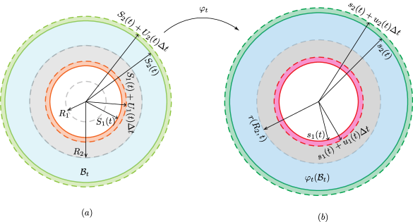
Figure 4: Cross sections of the reference and current configurations of an accreting-ablating thick hollow cylinder. (a) The material manifold $(\mathcal{B}_{t},\mathbf{G})$ at time $t$ has inner radial coordinate $S_{1}(t)$ and outer radial coordinate $S_{2}(t)$. Accretion is occurring on the outer surface and ablation on the inner surface. At time $t+\Delta t$, the inner radial coordinate is $S_{1}(t)+U_{1}(t)\Delta t$ and the outer radial coordinate is $S_{2}(t)+U_{2}(t)\Delta t$. (b) The deformed bar at time $t$ has inner radius $s_{1}(t)$ and outer radius $s_{2}(t)$. At time $t+\Delta t$, the inner radius is $s_{1}(t)+u_{1}(t)\Delta t$ and the outer radius is $s_{2}(t)+u_{2}(t)\Delta t$.

3.1 Kinematics

Let us consider a hollow circular cylindrical bar with initial length $L$, inner radius $R_{1}$ and outer radius $R_{2}>R_{1}$. We assume a homogeneous isotropic and incompressible material with an energy function $W=W(I_{1},I_{2})$, and use the cylindrical coordinates $(R,\Theta,Z)$ in the reference configuration, and cylindrical coordinates $(r,\theta,z)$ in the current configuration. The metric of the current configuration has the following representation

$$\mathbf{g}=\begin{bmatrix}1&0&0\\ 0&r^{2}&0\\ 0&0&1\end{bmatrix}\,.$$ (3.1)

Accretion is assumed to occur on the outer cylindrical boundary in the current configuration. The outer radius of the deformed body is denoted by $s_{2}(t)$ (Fig. 4). Ablation is assumed to occur on the inner cylindrical boundary of the current configuration that has the radius $s_{1}(t)$. Let us assign a time of attachment $\accentset{+}{\tau}(R)$ and a time of detachment ${\accentset{-}{\tau}}(R)$ to each layer with the radial coordinate $R>R_{1}$ in the reference configuration. Notice that for $R_{1}\leq R\leq R_{2}$, $\accentset{+}{\tau}(R)=0$. Hence, $\accentset{+}{\tau}(R)$ is invertible for $R\geq R_{2}$, while ${\accentset{-}{\tau}}(R)$ is invertible for $R\geq R_{1}$. We assume that $\accentset{-}{\tau}$ and $\accentset{+}{\tau}$ are diffeomorphisms with non-vanishing derivatives. Their inverses are denoted by $S_{1}=\accentset{-}{\tau}^{-1}$, and $S_{2}=\accentset{+}{\tau}^{-1}$, so that

$$s_{1}(t)=r(S_{1}(t),t)\,,\qquad s_{2}(t)=r(S_{2}(t),t)\,.$$ (3.2)

We also assume that accretion and ablation take place continuously in the time interval $t\in(0,T]$. It is assumed that the accreting-ablating body has non-vanishing volume at all times, i.e., $S_{1}(t)<S_{2}(t)$, $\forall~{}t\in(0,T]$. Let us consider a time-dependent finite extension of the bar such that it is slow enough for the inertial effects to be negligible and assume the following deformation mapping

$$r=r(R,t)\,,\quad\theta=\Theta\,,\quad z=\lambda^{2}(t)Z\,,$$ (3.3)

where $\lambda^{2}(t)$ is the axial stretch and is an unknown function to be determined. The deformation gradient reads

$$\mathbf{F}=\mathbf{F}(R,t)=\begin{bmatrix}r_{,R}(R,t)&0&0\\ 0&1&0\\ 0&0&\lambda^{2}(t)\end{bmatrix}\,.$$ (3.4)

3.2 The material metric

Let us define the following functions

$$\accentset{-}{r}(R)=r(R,{\accentset{-}{\tau}}(R))\,,\qquad\accentset{+}{r}(R)=r(R,\accentset{+}{\tau}(R))\,,\qquad\accentset{-}{\lambda}(R)=\lambda({\accentset{-}{\tau}}(R))\,,\qquad\accentset{+}{\lambda}(R)=\lambda(\accentset{+}{\tau}(R))\,.$$ (3.5)

We assume that the accreted cylindrical layer at any instant of time $t$ is stress-free. In other words, stress-free cylindrical layers are continuously added to the outer cylindrical boundary of the bar. This implies that the material metric at $R=S_{2}(t)$ is the pull-back of the metric of the (Euclidean) ambient space, i.e.,

$$\mathbf{G}(S_{2}(t))=\varphi_{t}^{*}\mathbf{g}(r(S_{2}(t),t))\,,~{}~{}\text{or}\qquad\mathbf{G}(R)=\varphi_{\accentset{+}{\tau}(R)}^{*}\,\mathbf{g}(r(R,\accentset{+}{\tau}(R)))\,.$$ (3.6)

In components, $G_{AB}(S_{2}(t))=G_{AB}(R)=F^{a}{}_{A}(R,\accentset{+}{\tau}(R))\,F^{b}{}_{B}(R,\accentset{+}{\tau}(R))\,g_{ab}(r(R,\accentset{+}{\tau}(R)))$. For this accretion-ablation problem, the material manifold (the natural configuration of the body) is an evolving Riemannian manifold $(\mathcal{B}_{t},\mathbf{G})$ with

$$\mathcal{B}_{t}=\left\{(R,\Theta,Z):0\leq\Theta<2\pi\,,S_{1}(t)\leq R\leq S_{2}(t)\,,~{}0\leq Z\leq L\right\}\,.$$ (3.7)

The reference configuration is equipped with the following material metric:

$$\mathbf{G}(R)=\begin{cases}\;\begin{bmatrix}1&0&0\\ 0&R^{2}&0\\ 0&0&1\end{bmatrix}\,,&\quad S_{1}(t)\leq R<R_{2}\,,\\ &\\ \begin{bmatrix}[r_{,R}(R,\accentset{+}{\tau}(R))]^{2}&0&0\\ 0&\accentset{+}{r}^{2}(R)&0\\ 0&0&\lambda^{4}(\accentset{+}{\tau}(R))\end{bmatrix}\,,&\quad R_{2}\leq R\leq S_{2}(t)\,.\end{cases}$$ (3.8)

Observe that $t_{\text{ablation}}:=\accentset{-}{\tau}(R_{2})$ is the time when the initial body is completely ablated.

3.3 The incompressibility constraint

The Jacobian is calculated as

$$J(R,t)=\sqrt{\frac{\det\mathbf{g}}{\det\mathbf{G}}}\det\mathbf{F}=\begin{cases}\displaystyle\frac{\lambda^{2}(t)\,r(R,t)\,r_{,R}(R,t)}{R}\,,&S_{1}(t)<R\leq R_{2}\,,\\[10.0pt] \displaystyle\frac{\lambda^{2}(t)\,r(R,t)\,r_{,R}(R,t)}{\accentset{+}{\lambda}^{2}(R)\,\accentset{+}{r}(R)\,r_{,R}(R,\accentset{+}{\tau}(R))}\,,&R_{2}\leq R<S_{2}(t)\,.\end{cases}$$ (3.9)

When $t<t_{\text{ablation}}$, incompressibility in the region $S_{1}(t)\leq R\leq R_{2}$ gives us

$$r(R,t)\,r_{,R}(R,t)=\frac{R}{\lambda^{2}(t)}\,,$$ (3.10)

thus implying that

$$r^{2}(R,t)=s_{1}^{2}(t)+\frac{R^{2}-S_{1}^{2}(t)}{\lambda^{2}(t)}\,.$$ (3.11)

Similarly, for the region $R_{2}\leq R\leq S_{2}(t)$, incompressibility requires that

$$\lambda^{2}(t)\,r(R,t)\,r_{,R}(R,t)=\accentset{+}{\lambda}^{2}(R)\,\accentset{+}{r}(R)\,r_{,R}(R,\accentset{+}{\tau}(R))\,,$$ (3.12)

which can be integrated to obtain

$$r^{2}(R,t)=r^{2}(R_{2},t)+\frac{2}{\lambda^{2}(t)}\int_{R_{2}}^{R}\accentset{+}{\lambda}^{2}(\xi)\,\accentset{+}{r}(\xi)\,r_{,R}(\xi,\accentset{+}{\tau}(\xi))\text{d}\xi\,,$$ (3.13)

for $t<t_{\text{ablation}}$. Equivalently, one may integrate (3.12) from $R$ to $S_{2}(t)$ to obtain:

$$r^{2}(R,t)=s_{2}^{2}(t)-\frac{2}{\lambda^{2}(t)}\int_{R}^{S_{2}(t)}\accentset{+}{\lambda}^{2}(\xi)\,\accentset{+}{r}(\xi)\,r_{,R}(\xi,\accentset{+}{\tau}(\xi))\text{d}\xi\,,$$ (3.14)

for $R\geq R_{2}$. Note that (3.14) holds for all $t>0$.

3.4 The accretion and ablation velocities

The accretion surfaces in the reference and the current configurations have the following representations:

$$\accentset{+}{\Omega}_{t} =\left\{(S_{1}(t),\Theta,Z):0\leq\Theta<2\pi\,,0\leq Z\leq L\right\}\,,$$ (3.15)

$$\accentset{+}{\omega}_{t} =\left\{(s_{1}(t),\Theta,\lambda^{2}(t)Z):0\leq\Theta<2\pi\,,0\leq Z\leq L\right\}\,.$$

The ablation surfaces in the reference and the current configurations are represented as:

$$\accentset{-}{\Omega}_{t} =\left\{(S_{2}(t),\Theta,Z):0\leq\Theta<2\pi\,,0\leq Z\leq L\right\}\,,$$ (3.16)

$$\accentset{-}{\omega}_{t} =\left\{(s_{2}(t),\Theta,\lambda^{2}(t)Z):0\leq\Theta<2\pi\,,0\leq Z\leq L\right\}\,.$$

Thus

$$\dot{s_{1}}(t)=r_{,R}(S_{1}(t),t)~{}U_{1}(t)+V(S_{1}(t),t)\,,$$ (3.17)

$$\dot{s_{2}}(t)=r_{,R}(S_{2}(t),t)~{}U_{2}(t)+V(S_{2}(t),t)\,,$$

where $U_{1}(t)=\dot{S_{1}}(t)>0$, and $U_{2}(t)=\dot{S_{2}}(t)>0$, i.e., both accretion and ablation surfaces are moving radially outward. Here, $V=\displaystyle\frac{\partial r}{\partial t}$ is the radial component of the material velocity on the accretion/ablation surface. We denote the ablation and accretion velocities by $u_{1}(t)$ and $u_{2}(t)$, respectively, which are defined as

$$u_{1}(t)=r_{,R}(S_{1}(t),t)\,U_{1}(t)\,,\qquad u_{2}(t)=r_{,R}(S_{2}(t),t)\,U_{2}(t)\,.$$ (3.18)

The choices $U_{1}(t)=u_{1}(t)$, and $U_{2}(t)=u_{2}(t)$ impose the following constraints on $r(R,t)$:

$$r_{,R}(S_{1}(t),t) =1\,,\quad\text{or}\qquad r_{,R}(R,\accentset{+}{\tau}(R))=1\,,$$ (3.19)

$$r_{,R}(S_{2}(t),t) =1\,,\quad\text{or}\qquad r_{,R}(R,{\accentset{-}{\tau}}(R))=1\,.$$

In particular, the choice (3.19)₁ makes the material metric $\mathbf{G}(R,t)$ and the Jacobian $J(R,t)$ continuous at $R=R_{2}$. Now, (3.19)₁ and (3.13) imply that for $t<t_{\text{ablation}}$

$$r^{2}(R,t)=r^{2}(R_{2},t)+\frac{2}{\lambda^{2}(t)}\int_{R_{2}}^{R}\accentset{+}{\lambda}^{2}(\xi)\,\accentset{+}{r}(\xi)\,\text{d}\xi\,.$$ (3.20)

Since $r(R,t)$ is continuous at $R=R_{2}$, (3.11) and (3.20) imply that

$$r^{2}(R,t)=s_{1}^{2}(t)+\frac{R_{2}^{2}-S_{1}^{2}(t)}{\lambda^{2}(t)}+\frac{2}{\lambda^{2}(t)}\int_{R_{2}}^{R}\accentset{+}{\lambda}^{2}(\xi)\,\accentset{+}{r}(\xi)\,\text{d}\xi\,,$$ (3.21)

for $R_{2}\leq R\leq S_{2}(t)$ with $t<t_{\text{ablation}}$. Substituting $R=S_{2}(t)$ in (3.21), one obtains

$$s_{1}^{2}(t)=s_{2}^{2}(t)-\frac{R_{2}^{2}-S_{1}^{2}(t)}{\lambda^{2}(t)}-\frac{2}{\lambda^{2}(t)}\int_{R_{2}}^{S_{2}(t)}\accentset{+}{\lambda}^{2}(\xi)\,\accentset{+}{r}(\xi)\,\text{d}\xi\,.$$ (3.22)

Now, one may substitute (3.22) into (3.11) and combine with (3.14) to write the kinematics in terms of $\accentset{+}{r}$ and $\accentset{+}{\lambda}$. As $s_{2}(t)=r(S_{2}(t),t)=\accentset{+}{r}(S_{2}(t))$, when $t<t_{\text{ablation}}$:

$$r^{2}(R,t)=\begin{dcases}\accentset{+}{r}^{2}(S_{2}(t))-\frac{R_{2}^{2}-R^{2}}{\lambda^{2}(t)}-\frac{2}{\lambda^{2}(t)}\int_{R_{2}}^{S_{2}(t)}\accentset{+}{\lambda}^{2}(\xi)\,\accentset{+}{r}(\xi)\,\text{d}\xi\,,&R\leq R_{2}\,,\\ \accentset{+}{r}^{2}(S_{2}(t))-\frac{2}{\lambda^{2}(t)}\int_{R}^{S_{2}(t)}\accentset{+}{\lambda}^{2}(\xi)\,\accentset{+}{r}(\xi)\,\text{d}\xi\,,&R\geq R_{2}\,.\end{dcases}$$ (3.23)

For $t\geq t_{\text{ablation}}$:

$$r^{2}(R,t)=\accentset{+}{r}^{2}(S_{2}(t))-\frac{2}{\lambda^{2}(t)}\int_{R}^{S_{2}(t)}\accentset{+}{\lambda}^{2}(\xi)\,\accentset{+}{r}(\xi)\,\text{d}\xi\,.$$ (3.24)

In a force-control problem, the functions $r(R,t)$ and $\lambda(t)$ are not known. However, it can be inferred from (3.23)-(3.24) that the knowledge of $\accentset{+}{r}(R)$ and $\lambda(t)$ is sufficient to calculate $r(R,t)$. Since $\accentset{+}{\tau}(R)$ is assumed to be given, $\accentset{+}{\lambda}(R)=\lambda(\accentset{+}{\tau}(R))$ is not an independent function. Thus, $\accentset{+}{r}(R)$ and $\lambda(t)$ are the only independent functions. Since $\lambda(t)$ is given in a displacement-control problem, $\accentset{+}{r}(R)$ is the only independent unknown function in displacement-control problems.

3.5 Stress calculation

In this section, we compute the stresses for both $t<t_{\text{ablation}}$ and $t>t_{\text{ablation}}$. The stresses are calculated separately for the initial and the accreted parts of the body. The radial equilibrium equation reads $\frac{\partial\sigma^{rr}}{\partial r}+\frac{1}{r}\sigma^{rr}-r\sigma^{\theta\theta}=0$. In terms of reference coordinates, $\frac{1}{r_{,R}}\frac{\partial\sigma^{rr}}{\partial R}+\frac{\sigma^{rr}}{r}-r\sigma^{\theta\theta}=0$. Thus, we have

$$\sigma^{rr}_{,R}(R,t)=\left[r^{2}(R,t)\sigma^{\theta\theta}(R,t)-\sigma^{rr}(R,t)\right]\frac{r_{,R}(R,t)}{r(R,t)}\,.$$ (3.25)

Recall that $\mathbf{b}^{\sharp}$ has components $b^{ab}=F^{a}{}_{A}\,F^{b}{}_{B}\,G^{AB}$ and $\mathbf{c}^{\sharp}$ has components $c^{ab}=g^{am}g^{bn}c_{mn}$, where $c_{ab}=F^{-A}{}_{a}\,F^{-B}{}_{b}\,G_{AB}$. For $S_{1}(t)\leq R\leq R_{2}$, and $t<t_{\text{ablation}}$:

$$\mathbf{b}^{\sharp}(R,t)=\begin{bmatrix}r_{,R}^{2}(R,t)&0&0\\ 0&\displaystyle\frac{1}{R^{2}}&0\\ 0&0&\lambda^{4}(t)\\ \end{bmatrix}\,,\qquad\mathbf{c}^{\sharp}(R,t)=\begin{bmatrix}\displaystyle\frac{1}{r_{,R}^{2}(R,t)}&0&0\\ 0&\displaystyle\frac{R^{2}}{r^{4}(R,t)}&0\\ 0&0&\displaystyle\frac{1}{\lambda^{4}(t)}\\ \end{bmatrix}\,.$$ (3.26)

The principal invariants of $\mathbf{b}$ read

$$I_{1}(R,t) =r_{,R}^{2}(R,t)+\frac{r^{2}(R,t)}{R^{2}}+\lambda^{4}(t)\,,$$ (3.27)

$$I_{2}(R,t) =r_{,R}^{2}(R,t)\,\lambda^{4}(t)+\frac{r_{,R}^{2}(R,t)\,r^{2}(R,t)}{R^{2}}+\frac{r^{2}(R,t)\,\lambda^{4}(t)}{R^{2}}\,.$$

The Cauchy stress has the following non-zero components

$$\sigma^{rr}(R,t) =-p(R,t)+\alpha(R,t)\,r_{,R}^{2}(R,t)-\frac{\beta(R,t)}{r_{,R}^{2}(R,t)}\,,$$ (3.28)

$$\sigma^{\theta\theta}(R,t) =-\frac{p(R,t)}{r^{2}(R,t)}+\frac{\alpha(R,t)}{R^{2}}-\frac{\beta(R,t)\,R^{2}}{r^{4}(R,t)}\,,$$

$$\sigma^{zz}(R,t) =-p(R,t)+\alpha(R,t)\,\lambda^{4}(t)-\,\frac{\beta(R,t)}{\lambda^{4}(t)}\,,$$

where $\alpha=2\frac{\partial W}{\partial I_{1}}$ and $\beta=2\frac{\partial W}{\partial I_{2}}$. Using the incompressibility constraint (3.10) each of the components of $\bm{\sigma}(R,t)$ can be expressed solely in terms of the kinematic quanities $r(R,t)$ and $\lambda(t)$, i.e., one can eliminate $r_{,R}(R,t)$ in (3.28)₁ to obtain

$$\sigma^{rr}(R,t)=-p(R,t)+\frac{R^{2}\alpha(R,t)}{r^{2}(R,t)\lambda^{4}(t)}-\frac{\beta(R,t)r^{2}(R,t)\lambda^{4}(t)}{R^{2}}\,.$$ (3.29)

Substituting (3.29) and (3.28)₂ in (3.25), one obtains

$$\sigma^{rr}_{,R}(R,t)=\frac{r^{4}(R,t)\lambda^{4}(t)-R^{4}}{R\,r^{4}(R,t)\lambda^{2}(t)}\left[\frac{\alpha(R,t)}{\lambda^{4}(t)}+\beta(R,t)\right]\,.$$ (3.30)

Since $\sigma^{rr}(S_{1}(t),t)=0$, it is implied that

$$\sigma^{rr}(R,t)=\int_{S_{1}(t)}^{R}\frac{r^{4}(\xi,t)\lambda^{4}(t)-\xi^{4}}{\xi\,r^{4}(\xi,t)\lambda^{2}(t)}\left[\frac{\alpha(\xi,t)}{\lambda^{4}(t)}+\beta(\xi,t)\right]d\xi\,,$$ (3.31)

for $S_{1}(t)\leq R\leq R_{2}$ and $t<t_{\text{ablation}}$. Thus, (3.29) gives the following expression for pressure

$$p(R,t)=\frac{R^{2}\alpha(R,t)}{r^{2}(R,t)\lambda^{4}(t)}-\frac{\beta(R,t)r^{2}(R,t)\lambda^{4}(t)}{R^{2}}-\int_{S_{1}(t)}^{R}\frac{r^{4}(\xi,t)\lambda^{4}(t)-\xi^{4}}{\xi\,r^{4}(\xi,t)\lambda^{2}(t)}\left[\frac{\alpha(\xi,t)}{\lambda^{4}(t)}+\beta(\xi,t)\right]d\xi\,.$$ (3.33)

Substituting (3.33) into (3.28)_2-3, one obtains

$$\hat{\sigma}^{\theta\theta}(R,t)= \frac{r^{4}(R,t)\lambda^{4}(t)-R^{4}}{R^{2}\,r^{2}(R,t)}\left[\frac{\alpha(R,t)}{\lambda^{4}(t)}+\beta(R,t)\right]+\int_{S_{1}(t)}^{R}\frac{r^{4}(\xi,t)\lambda^{4}(t)-\xi^{4}}{\xi\,r^{4}(\xi,t)\lambda^{2}(t)}\left[\frac{\alpha(\xi,t)}{\lambda^{4}(t)}+\beta(\xi,t)\right]d\xi\,,$$ (3.34)

$$\sigma^{zz}(R,t)= \alpha(R,t)\left[\lambda^{4}(t)-\frac{R^{2}}{r^{2}(R,t)\lambda^{4}(t)}\right]+\beta(R,t)\left[\frac{r^{2}(R,t)\lambda^{4}(t)}{R^{2}}-\frac{1}{\lambda^{4}(t)}\right]$$

$$+\int_{S_{1}(t)}^{R}\frac{r^{4}(\xi,t)\lambda^{4}(t)-\xi^{4}}{\xi\,r^{4}(\xi,t)\lambda^{2}(t)}\left[\frac{\alpha(\xi,t)}{\lambda^{4}(t)}+\beta(\xi,t)\right]d\xi\,.$$

For $\big{\{}R_{2}\leq R\leq S_{2}(t),\,t<t_{\text{ablation}}\big{\}}$, or $\big{\{}t\geq t_{\text{ablation}},\,S_{1}(t)\leq R\leq S_{2}(t)\big{\}}$:

$$\mathbf{b}^{\sharp}(R,t)=\begin{bmatrix}\displaystyle\left[\frac{r_{,R}(R,t)}{r_{,R}(R,\accentset{+}{\tau}(R))}\right]^{2}&0&0\\ 0&\displaystyle\frac{1}{\accentset{+}{r}^{2}(R)}&0\\ 0&0&\displaystyle\frac{\lambda^{4}(t)}{\accentset{+}{\lambda}^{4}(R)}\\ \end{bmatrix}\,,\quad\mathbf{c}^{\sharp}(R,t)=\begin{bmatrix}\displaystyle\left[\frac{r_{,R}(R,\accentset{+}{\tau}(R))}{r_{,R}(R,t)}\right]^{2}&0&0\\ 0&\displaystyle\frac{\accentset{+}{r}^{2}(R)}{r^{4}(R,t)}&0\\ 0&0&\displaystyle\frac{\accentset{+}{\lambda}^{4}(R)}{\lambda^{4}(t)}\\ \end{bmatrix}\,.$$ (3.35)

The principal invariants of $\mathbf{b}$ read

$$I_{1}(R,t) =r_{,R}^{2}(R,t)+\frac{r^{2}(R,t)}{\accentset{+}{r}^{2}(R)}+\frac{\lambda^{4}(t)}{\accentset{+}{\lambda}^{4}(R)}\;,$$ (3.36)

$$I_{2}(R,t) =\frac{r_{,R}^{2}(R,t)\,r^{2}(R,t)}{\accentset{+}{r}^{2}(R)}+\frac{r^{2}(R,t)\,\lambda^{4}(t)}{\accentset{+}{r}^{2}(R)\accentset{+}{\lambda}^{4}(R)}+\frac{r_{,R}^{2}(R,t)\lambda^{4}(t)}{\accentset{+}{\lambda}^{4}(R)}\,.$$

The non-zero components of the Cauchy stress are

$$\sigma^{rr}(R,t) =-p(R,t)+\alpha(R,t)r_{,R}^{2}(R,t)-\frac{\beta(R,t)}{r_{,R}^{2}(R,t)}\,,$$ (3.37)

$$\sigma^{\theta\theta}(R,t) =-\frac{p(R,t)}{r^{2}(R,t)}+\frac{\alpha(R,t)}{\accentset{+}{r}^{2}(R)}-\frac{\beta(R,t)\,\accentset{+}{r}^{2}(R)}{r^{4}(R,t)}\,,$$

$$\sigma^{zz}(R,t) =-p(R,t)+\frac{\alpha(R,t)\,\lambda^{4}(t)}{\accentset{+}{\lambda}^{4}(R)}-\frac{\beta(R,t)\,\accentset{+}{\lambda}^{4}(R)}{\lambda^{4}(t)}\,.$$

Using the constraints (3.12) and (3.19), each of the components of $\bm{\sigma}(R,t)$ can be expressed solely in terms of the kinematic quanities $r(R,t)$ and $\lambda(t)$, i.e., one can eliminate $r_{,R}(R,t)$ in (3.37)₁ to obtain

$$\sigma^{rr}(R,t)=-p(R,t)+\frac{\alpha(R,t)\,\accentset{+}{r}^{2}(R)\accentset{+}{\lambda}^{4}(R)}{r^{2}(R,t)\lambda^{4}(t)}-\frac{\beta(R,t)r^{2}(R,t)\,\lambda^{4}(t)}{\accentset{+}{r}^{2}(R)\,\accentset{+}{\lambda}^{4}(R)}\,.$$ (3.38)

Substituting (3.37)_1-2 in (3.25), one obtains

$$\sigma^{rr}_{,R}(R,t)=\frac{\accentset{+}{\lambda}^{2}(R)\left[r^{4}(R,t)\lambda^{4}(t)-\accentset{+}{r}^{4}(R)\accentset{+}{\lambda}^{4}(R)\right]}{r^{4}(R,t)\lambda^{2}(t)\,\accentset{+}{r}(R)}\left[\frac{\alpha(R,t)}{\lambda^{4}(t)}+\frac{\beta(R,t)}{\accentset{+}{\lambda}^{4}(R)}\right].$$ (3.39)

Since $\sigma^{rr}(S_{2}(t),t)=0$, it is implied that

$$\sigma^{rr}(R,t)=-\int_{R}^{S_{2}(t)}\frac{\accentset{+}{\lambda}^{2}(\xi)\left[r^{4}(\xi,t)\lambda^{4}(t)-\accentset{+}{r}^{4}(\xi)\accentset{+}{\lambda}^{4}(\xi)\right]}{r^{4}(\xi,t)\lambda^{2}(t)\,\accentset{+}{r}(\xi)}\left[\frac{\alpha(\xi,t)}{\lambda^{4}(t)}+\frac{\beta(\xi,t)}{\accentset{+}{\lambda}^{4}(\xi)}\right]d\xi\,,$$ (3.40)

whenever $\big{\{}R_{2}\leq R\leq S_{2}(t),\,t<t_{\text{ablation}}\big{\}}$, or $\big{\{}t\geq t_{\text{ablation}},\,S_{1}(t)\leq R\leq S_{2}(t)\big{\}}$. Thus, (3.38) gives the following expression for the pressure field

$$p(R,t) =\frac{\alpha(R,t)\accentset{+}{r}^{2}(R)\accentset{+}{\lambda}^{4}(R)}{r^{2}(R,t)\lambda^{4}(t)}-\frac{\beta(R,t)r^{2}(R,t)\lambda^{4}(t)}{\accentset{+}{r}^{2}(R)\accentset{+}{\lambda}^{4}(R)}$$ (3.41)

$$\quad+\int_{R}^{S_{2}(t)}\frac{\accentset{+}{\lambda}^{2}(\xi)\left[r^{4}(\xi,t)\lambda^{4}(t)-\accentset{+}{r}^{4}(\xi)\accentset{+}{\lambda}^{4}(\xi)\right]}{r^{4}(\xi,t)\lambda^{2}(t)\,\accentset{+}{r}(\xi)}\left[\frac{\alpha(\xi,t)}{\lambda^{4}(t)}+\frac{\beta(\xi,t)}{\accentset{+}{\lambda}^{4}(\xi)}\right]d\xi\,.$$

Substituting (3.41) into (3.37)_2-3, one obtains

$$\hat{\sigma}^{\theta\theta}(R,t)= \frac{r^{4}(R,t)\lambda^{4}(t)-\accentset{+}{r}^{4}(R)\accentset{+}{\lambda}^{4}(R)}{r^{2}(R,t)\accentset{+}{r}^{2}(R)}\left[\frac{\alpha(R,t)}{\lambda^{4}(t)}+\frac{\beta(R,t)}{\accentset{+}{\lambda}^{4}(R)}\right]$$ (3.42)

$$-\int_{R}^{S_{2}(t)}\frac{\accentset{+}{\lambda}^{2}(\xi)\left[r^{4}(\xi,t)\lambda^{4}(t)-\accentset{+}{r}^{4}(\xi)\accentset{+}{\lambda}^{4}(\xi)\right]}{r^{4}(\xi,t)\lambda^{2}(t)\accentset{+}{r}(\xi)}\left[\frac{\alpha(\xi,t)}{\lambda^{4}(t)}+\frac{\beta(\xi,t)}{\accentset{+}{\lambda}^{4}(\xi)}\right]d\xi\,,$$

$$\sigma^{zz}(R,t)= \alpha(R,t)\left[\frac{\lambda^{4}(t)}{\accentset{+}{\lambda}^{4}(R)}-\frac{\accentset{+}{\lambda}^{4}(R)\accentset{+}{r}^{2}(R)}{\lambda^{4}(t)r^{2}(R,t)}\right]+\beta(R,t)\left[\frac{\lambda^{4}(t)r^{2}(R,t)}{\accentset{+}{\lambda}^{4}(R)\accentset{+}{r}^{2}(R)}-\frac{\accentset{+}{\lambda}^{4}(R)}{\lambda^{4}(t)}\right]$$

$$-\int_{R}^{S_{2}(t)}\frac{\accentset{+}{\lambda}^{2}(\xi)\left[r^{4}(\xi,t)\lambda^{4}(t)-\accentset{+}{r}^{4}(\xi)\accentset{+}{\lambda}^{4}(\xi)\right]}{r^{4}(\xi,t)\lambda^{2}(t)\accentset{+}{r}(\xi)}\left[\frac{\alpha(\xi,t)}{\lambda^{4}(t)}+\frac{\beta(\xi,t)}{\accentset{+}{\lambda}^{4}(\xi)}\right]d\xi\,,$$

for $\big{\{}R_{2}\leq R\leq S_{2}(t),\,t<t_{\text{ablation}}\big{\}}$, and $\big{\{}t\geq t_{\text{ablation}},\,S_{1}(t)\leq R\leq S_{2}(t)\big{\}}$. Note that $\sigma^{\theta\theta}(S_{2}(t),t)=0$, and $\sigma^{zz}(S_{2}(t),t)=0$, i.e., $\bm{\sigma}(S_{2}(t),t)=\mathbf{0}$. Since $\sigma^{rr}(R,t)$ has to be continuous in $R$ at $R_{2}$ at any time $t<t_{\text{ablation}}$, we must have

$$\int_{S_{1}(t)}^{R_{2}}\frac{r^{4}(\xi,t)\lambda^{4}(t)-\xi^{4}}{\xi\,r^{4}(\xi,t)\lambda^{2}(t)}\left[\frac{\alpha(\xi,t)}{\lambda^{4}(t)}+\beta(\xi,t)\right]d\xi$$ (3.43)

$$\qquad+\int_{R_{2}}^{S_{2}(t)}\frac{\accentset{+}{\lambda}^{2}(\xi)\left[r^{4}(\xi,t)\lambda^{4}(t)-\accentset{+}{r}^{4}(\xi)\accentset{+}{\lambda}^{4}(\xi)\right]}{r^{4}(\xi,t)\lambda^{2}(t)\accentset{+}{r}(\xi)}\left[\frac{\alpha(\xi,t)}{\lambda^{4}(t)}+\frac{\beta(\xi,t)}{\accentset{+}{\lambda}^{4}(\xi)}\right]d\xi=0\,,$$

for all $0<t<t_{\text{ablation}}$.

Remark 3.1.

Using (3.40), one obtains

$$\sigma^{rr}(R_{2},t)=-\int_{R_{2}}^{S_{2}(t)}\frac{\accentset{+}{\lambda}^{2}(\xi)\left[r^{4}(\xi,t)\lambda^{4}(t)-\accentset{+}{r}^{4}(\xi)\accentset{+}{\lambda}^{4}(\xi)\right]}{r^{4}(\xi,t)\lambda^{2}(t)\accentset{+}{r}(\xi)}\left[\frac{\alpha(\xi,t)}{\lambda^{4}(t)}+\frac{\beta(\xi,t)}{\accentset{+}{\lambda}^{4}(\xi)}\right]d\xi\,,$$ (3.45)

which can be substituted into (3.32) to give

$$\sigma^{rr}(R,t)= -\int_{R}^{R_{2}}\frac{r^{4}(\xi,t)\lambda^{4}(t)-\xi^{4}}{\xi\,r^{4}(\xi,t)\lambda^{2}(t)}\left[\frac{\alpha(\xi,t)}{\lambda^{4}(t)}+\beta(\xi,t)\right]d\xi$$ (3.46)

$$-\int_{R_{2}}^{S_{2}(t)}\frac{\accentset{+}{\lambda}^{2}(\xi)\left[r^{4}(\xi,t)\lambda^{4}(t)-\accentset{+}{r}^{4}(\xi)\accentset{+}{\lambda}^{4}(\xi)\right]}{r^{4}(\xi,t)\lambda^{2}(t)\accentset{+}{r}(\xi)}\left[\frac{\alpha(\xi,t)}{\lambda^{4}(t)}+\frac{\beta(\xi,t)}{\accentset{+}{\lambda}^{4}(\xi)}\right]d\xi\,,$$

where $S_{1}(t)\leq R\leq R_{2}$, and $t<t_{\text{ablation}}$. Thus, (3.29) gives the following expression for the pressure field

$$p(R,t) =\frac{R^{2}\alpha(R,t)}{r^{2}(R,t)\lambda^{4}(t)}-\frac{\beta(R,t)r^{2}(R,t)\lambda^{4}(t)}{R^{2}}+\int_{R}^{R_{2}}\frac{r^{4}(\xi,t)\lambda^{4}(t)-\xi^{4}}{\xi\,r^{4}(\xi,t)\lambda^{2}(t)}\left[\frac{\alpha(\xi,t)}{\lambda^{4}(t)}+\beta(\xi,t)\right]d\xi$$ (3.47)

$$\quad+\int_{R_{2}}^{S_{2}(t)}\frac{\accentset{+}{\lambda}^{2}(\xi)\left[r^{4}(\xi,t)\lambda^{4}(t)-\accentset{+}{r}^{4}(\xi)\accentset{+}{\lambda}^{4}(\xi)\right]}{r^{4}(\xi,t)\lambda^{2}(t)\accentset{+}{r}(\xi)}\left[\frac{\alpha(\xi,t)}{\lambda^{4}(t)}+\frac{\beta(\xi,t)}{\accentset{+}{\lambda}^{4}(\xi)}\right]d\xi\,,$$

where $S_{1}(t)\leq R\leq R_{2}$. Substituting (3.47) into (3.28)_2-3 one obtains

$$\hat{\sigma}^{\theta\theta}(R,t) =\frac{r^{4}(R,t)\lambda^{4}(t)-R^{4}}{R^{2}\,r^{2}(R,t)}\left[\frac{\alpha(R,t)}{\lambda^{4}(t)}+\beta(R,t)\right]-\int_{R}^{R_{2}}\frac{r^{4}(\xi,t)\lambda^{4}(t)-\xi^{4}}{\xi\,r^{4}(\xi,t)\lambda^{2}(t)}\left[\frac{\alpha(\xi,t)}{\lambda^{4}(t)}+\beta(\xi,t)\right]d\xi$$ (3.48)

$$\quad-\int_{R_{2}}^{S_{2}(t)}\frac{\accentset{+}{\lambda}^{2}(\xi)\left[r^{4}(\xi,t)\lambda^{4}(t)-\accentset{+}{r}^{4}(\xi)\accentset{+}{\lambda}^{4}(\xi)\right]}{r^{4}(\xi,t)\lambda^{2}(t)\accentset{+}{r}(\xi)}\left[\frac{\alpha(\xi,t)}{\lambda^{4}(t)}+\frac{\beta(\xi,t)}{\accentset{+}{\lambda}^{4}(\xi)}\right]d\xi,$$

$$\sigma^{zz}(R,t) =\alpha(R,t)\left[\lambda^{4}(t)-\frac{R^{2}}{r^{2}(R,t)\lambda^{4}(t)}\right]+\beta(R,t)\left[\frac{r^{2}(R,t)\lambda^{4}(t)}{R^{2}}-\frac{1}{\lambda^{4}(t)}\right]$$

$$\quad-\int_{R}^{R_{2}}\frac{r^{4}(\xi,t)\lambda^{4}(t)-\xi^{4}}{\xi\,r^{4}(\xi,t)\lambda^{2}(t)}\left[\frac{\alpha(\xi,t)}{\lambda^{4}(t)}+\beta(\xi,t)\right]d\xi$$

$$\quad-\int_{R_{2}}^{S_{2}(t)}\frac{\accentset{+}{\lambda}^{2}(\xi)\left[r^{4}(\xi,t)\lambda^{4}(t)-\accentset{+}{r}^{4}(\xi)\accentset{+}{\lambda}^{4}(\xi)\right]}{r^{4}(\xi,t)\lambda^{2}(t)\accentset{+}{r}(\xi)}\left[\frac{\alpha(\xi,t)}{\lambda^{4}(t)}+\frac{\beta(\xi,t)}{\accentset{+}{\lambda}^{4}(\xi)}\right]d\xi\,,$$

for $S_{1}(t)\leq R\leq R_{2}$. On the ablation boundary

$$\hat{\sigma}^{\theta\theta}(S_{1}(t),t) =\begin{cases}\displaystyle\left[\frac{s_{1}^{2}(t)\lambda^{4}(t)}{S_{1}^{2}(t)}-\frac{S_{1}^{2}(t)}{s_{1}^{2}(t)}\right]\left[\frac{\alpha(S_{1}(t),t)}{\lambda^{4}(t)}+\beta(S_{1}(t),t)\right]\,,&t<t_{\text{ablation}}\,,\\[10.0pt] \displaystyle\left[\frac{s_{1}^{2}(t)\lambda^{4}(t)}{\accentset{+}{r}^{2}(S_{1}(t))}-\frac{\accentset{+}{r}^{2}(S_{1}(t))\accentset{+}{\lambda}^{4}(S_{1}(t))}{s_{1}^{2}(t)}\right]\left[\frac{\alpha(S_{1}(t),t)}{\lambda^{4}(t)}+\frac{\beta(S_{1}(t),t)}{\accentset{+}{\lambda}^{4}(S_{1}(t))}\right]\,,&t\geq t_{\text{ablation}}\,,\\ \end{cases}$$ (3.49)

$$\sigma^{zz}(S_{1}(t),t) =\begin{cases}\displaystyle\left[\frac{s_{1}^{2}(t)\lambda^{4}(t)}{S_{1}^{2}(t)}-\frac{1}{\lambda^{4}(t)}\right]\left[\frac{\alpha(S_{1}(t),t)S_{1}^{2}(t)}{s_{1}^{2}(t)}+\beta(S_{1}(t),t)\right]\,,&t<t_{\text{ablation}}\,,\\[10.0pt] \displaystyle\alpha(S_{1}(t),t)\left[\frac{\lambda^{4}(t)}{\accentset{+}{\lambda}^{4}(S_{1}(t))}-\frac{\accentset{+}{\lambda}^{4}(S_{1}(t))\accentset{+}{r}^{2}(S_{1}(t))}{\lambda^{4}(t)s_{1}^{2}(t)}\right]&\\ \qquad\qquad+\beta(S_{1}(t),t)\left[\frac{\lambda^{4}(t)s_{1}^{2}(t)}{\accentset{+}{\lambda}^{4}(S_{1}(t))\accentset{+}{r}^{2}(S_{1}(t))}-\frac{\accentset{+}{\lambda}^{4}(S_{1}(t))}{\lambda^{4}(t)}\right]\,,&t\geq t_{\text{ablation}}\,.\\ \end{cases}$$

Notice that $\sigma^{\theta\theta}$ and $\sigma^{zz}$ do not vanish on the ablation boundary.

Remark 3.2.

In [Yavari et al., 2023] it was shown that the finite extension of an accreting circular cylindrical bar made of an arbitrary incompressible isotropic solid is a universal deformation even in the presence of radially-symmetric accretion. We have observed here that this result holds even when there is simultaneous radially-symmetric accretion and ablation on the outer and inner boundaries, respectively.

The applied axial force.

The axial force at the two ends of the bar is given by

$$F(t)=2\pi\int_{S_{1}(t)}^{S_{2}(t)}P^{zZ}(R,t)R\,\text{d}R\,,$$ (3.50)

where $P^{zZ}(R,t)=\displaystyle\frac{\sigma^{zz}(R,t)}{\lambda^{2}(t)}$ is the $zZ$-component of first Piola-Kirchhoff stress. For $S_{1}(t)\leq R\leq R_{2}$ and $t<t_{\text{ablation}}$:

$$P^{zZ}(R,t) =\alpha(R,t)\left[\lambda^{2}(t)-\frac{R^{2}}{r^{2}(R,t)\lambda^{6}(t)}\right]+\beta(R,t)\left[\frac{r^{2}(R,t)\lambda^{2}(t)}{R^{2}}-\frac{1}{\lambda^{6}(t)}\right]$$ (3.51)

$$\quad-\int_{R}^{R_{2}}\frac{r^{4}(\xi,t)\lambda^{4}(t)-\xi^{4}}{\xi\,r^{4}(\xi,t)\lambda^{4}(t)}\left[\frac{\alpha(\xi,t)}{\lambda^{4}(t)}+\beta(\xi,t)\right]d\xi$$

$$\quad-\int_{R_{2}}^{S_{2}(t)}\frac{\accentset{+}{\lambda}^{2}(\xi)\left[r^{4}(\xi,t)\lambda^{4}(t)-\accentset{+}{r}^{4}(\xi)\accentset{+}{\lambda}^{4}(\xi)\right]}{r^{4}(\xi,t)\lambda^{4}(t)\accentset{+}{r}(\xi)}\left[\frac{\alpha(\xi,t)}{\lambda^{4}(t)}+\frac{\beta(\xi,t)}{\accentset{+}{\lambda}^{4}(\xi)}\right]d\xi\,.$$

For $\big{\{}R_{2}\leq R\leq S_{2}(t),t<t_{\text{ablation}}\big{\}}$ and $\big{\{}t\geq t_{\text{ablation}},S_{1}(t)\leq R\leq S_{2}(t)\big{\}}$:

$$P^{zZ}(R,t) =\alpha(R,t)\left[\frac{\lambda^{2}(t)}{\accentset{+}{\lambda}^{4}(R)}-\frac{\accentset{+}{\lambda}^{4}(R)\,\accentset{+}{r}^{2}(R)}{\lambda^{6}(t)\,r^{2}(R,t)}\right]+\beta(R,t)\left[\frac{\lambda^{2}(t)\,r^{2}(R,t)}{\accentset{+}{\lambda}^{4}(R)\,\accentset{+}{r}^{2}(R)}-\frac{\accentset{+}{\lambda}^{4}(R)}{\lambda^{6}(t)}\right]$$ (3.52)

$$\quad-\int_{R}^{S_{2}(t)}\frac{\accentset{+}{\lambda}^{2}(\xi)\left[r^{4}(\xi,t)\,\lambda^{4}(t)-\accentset{+}{r}^{4}(\xi)\,\accentset{+}{\lambda}^{4}(\xi)\right]}{r^{4}(\xi,t)\,\lambda^{4}(t)\,\accentset{+}{r}(\xi)}\left[\frac{\alpha(\xi,t)}{\lambda^{4}(t)}+\frac{\beta(\xi,t)}{\accentset{+}{\lambda}^{4}(\xi)}\right]d\xi\,\,.$$

Remark 3.3.

Observe that (3.53) and (3.44) can be combined to define the following function

$$\Upsilon(t):=\begin{cases}\displaystyle\int_{S_{1}(t)}^{R_{2}}\frac{r^{4}(\xi,t)\lambda^{4}(t)-\xi^{4}}{\xi\,r^{4}(\xi,t)\lambda^{2}(t)}\left[\frac{\alpha(\xi,t)}{\lambda^{4}(t)}+\beta(\xi,t)\right]d\xi&\\ \quad\quad\displaystyle+\int_{R_{2}}^{S_{2}(t)}\frac{\accentset{+}{\lambda}^{2}(\xi)\left[r^{4}(\xi,t)\lambda^{4}(t)-\accentset{+}{r}^{4}(\xi)\accentset{+}{\lambda}^{4}(\xi)\right]}{r^{4}(\xi,t)\lambda^{2}(t)\accentset{+}{r}(\xi)}\left[\frac{\alpha(\xi,t)}{\lambda^{4}(t)}+\frac{\beta(\xi,t)}{\accentset{+}{\lambda}^{4}(\xi)}\right]d\xi\,,&t\leq t_{\text{ablation}}\,,\\[20.0pt] \displaystyle\int_{S_{1}(t)}^{S_{2}(t)}\frac{\accentset{+}{\lambda}^{2}(\xi)\left[r^{4}(\xi,t)\lambda^{4}(t)-\accentset{+}{r}^{4}(\xi)\accentset{+}{\lambda}^{4}(\xi)\right]}{r^{4}(\xi,t)\lambda^{2}(t)\,\accentset{+}{r}(\xi)}\left[\frac{\alpha(\xi,t)}{\lambda^{4}(t)}+\frac{\beta(\xi,t)}{\accentset{+}{\lambda}^{4}(\xi)}\right]d\xi\,,&t\geq t_{\text{ablation}}\,.\end{cases}$$ (3.53)

In a displacement-control problem, where $\lambda(t)$ is given, $\Upsilon(\accentset{+}{\tau}(R))=0$ is to be solved with $\accentset{+}{r}(R_{2})=R_{2}$ to find the unknown function $\accentset{+}{r}(R)$ for $R>R_{2}$.

3.6 The accretion-ablation initial-boundary-value problem for a neo-Hookean solid

Let $T\leq t_{\text{ablation}}$. Consider a homogeneous neo-Hookean material for which $\alpha(R,t)={\mu}(R)=\mu_{0}>0$ and $\beta(R,t)=0$. In order to simplify the calculations, assume that the spatial accretion/ablation velocities are constant, i.e., $u_{1}(t)=\accentset{-}{\upsilon}>0$ and $u_{2}(t)=\accentset{+}{\upsilon}>0$. The signs of $\accentset{+}{\upsilon}$ and $\accentset{-}{\upsilon}$ indicate that both accretion and ablation interfaces are moving radially outward. Thus,

$$S_{1}(t) =R_{1}+\accentset{-}{\upsilon}t\,,\quad\text{or}\qquad{\accentset{-}{\tau}}(R)=\frac{R-R_{1}}{\accentset{-}{\upsilon}}\,,$$ (3.54)

$$S_{2}(t) =R_{2}+\accentset{+}{\upsilon}t\,,\quad\text{or}\qquad\accentset{+}{\tau}(R)=\frac{R-R_{2}}{\accentset{+}{\upsilon}}\,.$$

The nonzero physical components of the Cauchy stress for this problem are listed as follows:

$$\sigma^{rr}(R,t) =\begin{dcases}\frac{\mu_{0}}{\lambda^{2}(t)}\int_{S_{1}(t)}^{R}\frac{\text{d}\xi}{\xi\,}-\frac{\mu_{0}}{\lambda^{6}(t)}\int_{S_{1}(t)}^{R}\frac{\xi^{3}\text{d}\xi}{r^{4}(\xi,t)}\,,&R<R_{2}\,,\\ -\frac{\mu_{0}}{\lambda^{2}(t)}\int_{R}^{S_{2}(t)}\frac{\accentset{+}{\lambda}^{2}(\xi)\text{d}\xi}{\accentset{+}{r}(\xi)}+\frac{\mu_{0}}{\lambda^{6}(t)}\int_{R}^{S_{2}(t)}\frac{\accentset{+}{r}^{3}(\xi)\accentset{+}{\lambda}^{6}(\xi)\text{d}\xi}{r^{4}(\xi,t)}\,,&R\geq R_{2}\,,\end{dcases}$$ (3.56)

$$\hat{\sigma}^{\theta\theta}(R,t) =\begin{dcases}\mu_{0}\left[\frac{r^{2}(R,t)}{R^{2}}-\frac{R^{2}}{\lambda^{4}(t)\,r^{2}(R,t)}\right]+\sigma^{rr}(R,t)\,,&R<R_{2}\,,\\ \mu_{0}\left[\frac{r^{2}(R,t)}{\accentset{+}{r}^{2}(R)}-\frac{\accentset{+}{\lambda}^{4}(R)\accentset{+}{r}^{2}(R)}{\lambda^{4}(t)r^{2}(R,t)}\right]+\sigma^{rr}(R,t)\,,&R\geq R_{2}\,,\end{dcases}$$

$$\sigma^{zz}(R,t) =\begin{dcases}\mu_{0}\left[\lambda^{4}(t)-\frac{R^{2}}{\lambda^{4}(t)r^{2}(R,t)}\right]+\sigma^{rr}(R,t)\,,&R<R_{2}\,,\\ \mu_{0}\left[\frac{\lambda^{4}(t)}{\accentset{+}{\lambda}^{4}(R)}-\frac{\accentset{+}{\lambda}^{4}(R)\accentset{+}{r}^{2}(R)}{\lambda^{4}(t)r^{2}(R,t)}\right]+\sigma^{rr}(R,t)\,,&R\geq R_{2}\,.\end{dcases}$$

Traction continuity equation (3.53) simplifies to read

$$\lambda^{4}(t)\left[\int_{S_{1}(t)}^{R_{2}}\frac{\text{d}\xi}{\xi}+\int_{R_{2}}^{S_{2}(t)}\frac{\accentset{+}{\lambda}^{2}(\xi)\text{d}\xi}{\accentset{+}{r}(\xi)}\right]=\int_{S_{1}(t)}^{R_{2}}\frac{\xi^{3}\text{d}\xi}{r^{4}(\xi,t)}+\int_{R_{2}}^{S_{2}(t)}\frac{\accentset{+}{r}^{3}(\xi)\accentset{+}{\lambda}^{6}(\xi)\text{d}\xi}{r^{4}(\xi,t)}\,.$$ (3.57)

Now, one can differentiate (3.57) with respect to $t$ and use (3.11) and (3.21) to deduce that (the detailed calculations are given in Appendix A)

$$\accentset{+}{r}(R)=\frac{R_{2}+\int_{R_{2}}^{R}\accentset{+}{\lambda}(\xi)\text{d}\xi}{\accentset{+}{\lambda}(R)}\,,$$ (3.58)

and

$$r(R,t)=\begin{cases}\displaystyle\frac{R}{\lambda(t)}\,,&S_{1}(t)\leq R\leq R_{2}\,,\\[10.0pt] \displaystyle\frac{\accentset{+}{\lambda}(R)\accentset{+}{r}(R)}{\lambda(t)}\,,&R_{2}\leq R\leq S_{2}(t)\,,\end{cases}$$ (3.59)

which when substituted into (3.56) implies that $\sigma^{rr}(R,t)=\sigma^{\theta\theta}(R,t)=0$. Morever,

$$P^{zZ}(R,t)=\begin{cases}\displaystyle\mu_{0}\left[\lambda^{2}(t)-\frac{1}{\lambda^{4}(t)}\right]\,,&S_{1}(t)\leq R\leq R_{2}\,,\\[10.0pt] \displaystyle\mu_{0}\left[\frac{\lambda^{2}(t)}{\accentset{+}{\lambda}^{4}(R)}-\frac{\accentset{+}{\lambda}^{2}(R)}{\lambda^{4}(t)}\right]\,,&R_{2}\leq R\leq S_{2}(t)\,,\end{cases}$$ (3.60)

using which the axial force can be expressed as

$$\frac{F(t)}{2\pi\mu_{0}}=\frac{R_{2}^{2}-S_{1}^{2}(t)}{2}\left[\lambda^{2}(t)-\frac{1}{\lambda^{4}(t)}\right]+\lambda^{2}(t)\int_{R_{2}}^{S_{2}(t)}\frac{R\,\text{d}R}{\accentset{+}{\lambda}^{4}(R)}-\frac{1}{\lambda^{4}(t)}\int_{R_{2}}^{S_{2}(t)}R\accentset{+}{\lambda}^{2}(R)\text{d}R\,.$$ (3.61)

In a force-control problem $F(t)$ is given (with $F(0)=0$), and $S_{1}(t)$, $S_{2}(t)$ are both known. All one needs to find is the unknown function $\lambda(t)$ that satisfies (3.61).

Example 3.4.

Consider a displacement-control problem with $R_{2}=2R_{1}$, $\accentset{-}{\upsilon}=2\frac{R_{1}}{T}$, $\accentset{+}{\upsilon}=3\frac{R_{1}}{T}$, and $\lambda(t)=1+a\left(\frac{t}{T}\right)^{n}$, where $n\geq 0$, and $a\in\mathbb{R}$. Then $t_{\text{ablation}}=\frac{T}{2}$ and $S_{2}(t_{\text{ablation}})=3.5R_{1}$. We solve this problem for $a\in\big{\{}\pm 1\big{\}}$ and $n\in\big{\{}\frac{1}{2},1,2\big{\}}$ assuming the numerical values $R_{1}=1$ and $T=1$. At any given $t<t_{\text{ablation}}$, $\sigma^{zz}(R,t)$ is constant in the initial body ($R\leq R_{2}$), as we have assumed the material to be homogeneous and the deformation to be uniform (Figs. 5 and 6). As foreseen, $\sigma^{zz}\geq 0$ for $\lambda\geq 1$ (Fig. 5) and $\sigma^{zz}\leq 0$ for $\lambda\leq 1$ (Fig. 6). Further, $\sigma^{zz}$ is nonzero on the ablation boundary (Fig. 7). Note that $\dot{\lambda}(t)$ taken in this example blows up near $t=0$ for $n<1$ and $a>0$. This is why when the bar is subjected to the elongation $\lambda(t)=1+\sqrt{\frac{t}{T}}$ , we first observe a reduction in the outer diameter $\accentset{+}{r}(R)$, or equivalently $s_{2}(t)$, see Fig. 5. Later, as the rate of elongation reduces, this effect is overshadowed by accretion and $\accentset{+}{r}(R)$ increases monotonically.

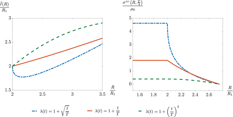
Figure 5: Solution to the displacement-control problem described in Example 3.4 for $a=1$. For $\lambda(t)=1+\left(\frac{t}{T}\right)^{n}$ (an increasing function) the variation of the axial stress $\sigma^{zz}(R,t)$ with $R$ at $t=\frac{T}{4}$ for the cases $n\in\left\{\frac{1}{2},1,2\right\}$ is shown.

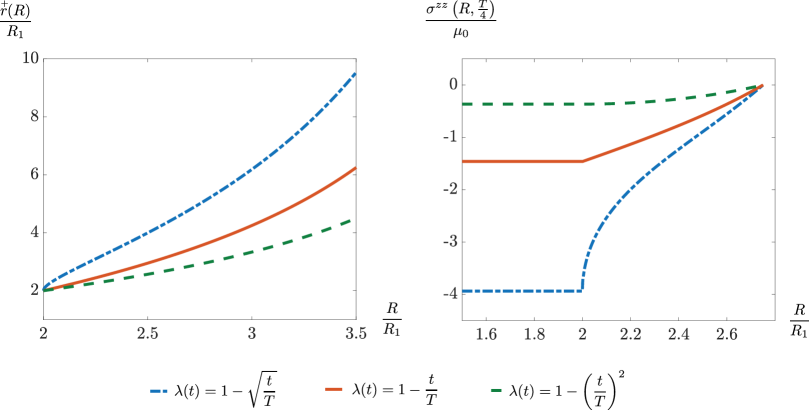
Figure 6: Solution to the displacement-control problem described in Example 3.4 for $a=-1$. For $\lambda(t)=1-\left(\frac{t}{T}\right)^{n}$ (a decreasing function) the variation of the axial stress $\sigma^{zz}(R,t)$ with $R$ at $t=\frac{T}{4}$ for the cases $n\in\left\{\frac{1}{2},1,2\right\}$ is shown.

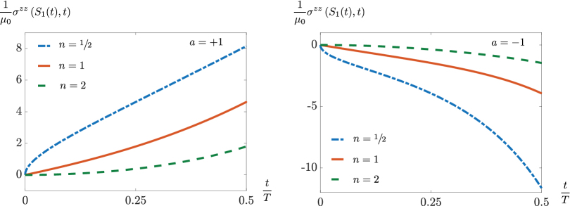
Figure 7: The axial stress on the ablation boundary for the displacement-control problem described in Example 3.4. The variation of $\sigma^{zz}(S_{1}(t),t)$ with $t(<t_{\text{ablation}})$ for $\lambda(t)=1+a\left(\frac{t}{T}\right)^{n}$, where $a\in\big{\{}\pm 1\big{\}}$ and $n\in\left\{\frac{1}{2},1,2\right\}$ is shown.

Example 3.5.

Consider a force-control problem with $R_{2}=2R_{1}$, $\accentset{-}{\upsilon}=\frac{R_{1}}{T}$, $\accentset{+}{\upsilon}=2\frac{R_{1}}{T}$. Then $t_{\text{ablation}}=T$ and $S_{2}(T)=4R_{1}$. To find solutions of the form (3.59), first define $h(t):=\int_{R_{2}}^{S_{2}(t)}\frac{R\,\text{d}R}{\accentset{+}{\lambda}^{4}(R)}$, and $k(t):=\int_{R_{2}}^{S_{2}(t)}R\accentset{+}{\lambda}^{2}(R)\text{d}R$, so that $\dot{h}(t)=\frac{\accentset{+}{\upsilon}S_{2}(t)}{\lambda^{4}(t)}$ and $\dot{k}(t)=\accentset{+}{\upsilon}S_{2}(t)\lambda^{2}(t)$. Differentiating (3.61) with respect to $t$, one obtains

$$\Bigg{[}2\lambda(t)\left[\frac{R_{2}^{2}-S_{1}^{2}(t)}{2}+h(t)\right]+\frac{4}{\lambda^{5}(t)}\left[\frac{R_{2}^{2}-S_{1}^{2}(t)}{2}+k(t)\right]\Bigg{]}\dot{\lambda}(t)+\accentset{-}{\upsilon}S_{1}(t)\left[\frac{1}{\lambda^{4}(t)}-\lambda^{2}(t)\right]=\frac{\dot{F}(t)}{2\pi\mu_{0}}\,.$$ (3.62)

Thus, we need to solve the following system of nonlinear ODEs:

$$\begin{cases}\displaystyle\dot{\lambda}(t)=\frac{f(t)+\accentset{-}{\upsilon}S_{1}(t)\left[\lambda^{2}(t)-\frac{1}{\lambda^{4}(t)}\right]}{2\lambda(t)\left[\frac{R_{2}^{2}-S_{1}^{2}(t)}{2}+h(t)\right]+\frac{4}{\lambda^{5}(t)}\left[\frac{R_{2}^{2}-S_{1}^{2}(t)}{2}+k(t)\right]}\,,\\ \displaystyle\dot{h}(t)=\frac{\accentset{+}{\upsilon}S_{2}(t)}{\lambda^{4}(t)}\,,\\ \displaystyle\dot{k}(t)=\accentset{+}{\upsilon}S_{2}(t)\lambda^{2}(t)\,,\\ \displaystyle\lambda(0)=1\,,~{}h(0)=0\,,~{}k(0)=0\,,\end{cases}$$ (3.63)

where $f(t):=\frac{\dot{F}(t)}{2\pi\mu_{0}}$. Assume the numerical values $R_{1}=1$ and $T=1$. The time-dependent force $F(t)$ is taken as a polynomial function of $t$ in Fig. 8, and an error function of $t$ in Fig. 9, and a sinusoidal function of $t$ in Fig. 10. The sign of $\sigma^{zz}$ is the same as that of $F$ for monotonic loads (Fig. 8). In Fig. 9, as $F(t)$ increases from $0$ until the asymptotic value $\mu_{0}\pi R_{1}^{2}$ is reached, $\dot{\lambda}(t)$ (and hence the axial strain rate) decreases until an asymptotic limit is reached. In Fig. 10 we look at three different time-dependent loads with $F(0)=F(T)=0$, but all of them have different stretches at $t=T$ because their loading histories are different. Similarly, $F(t)=\mu_{0}\pi R_{1}^{2}\sin(\frac{\pi t}{T})$ and $F(t)=\mu_{0}\pi R_{1}^{2}\sin^{2}(\frac{\pi t}{T})$ have the same load at $t=\frac{T}{2}$, but different radial variation of $\sigma^{zz}$ at that instant because of their different loading histories.

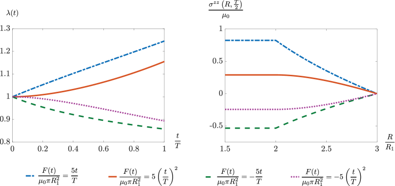
Figure 8: Solution to the force-control problem described in Example 3.5 with $\displaystyle F(t)=\pm 5\mu_{0}\pi R_{1}^{2}\left(\frac{t}{T}\right)^{n}$, where $n\in\{1,2\}$. The function $\lambda(t)$ reported here is the solution to the integral equation (3.61). The variation of the axial stress $\sigma^{zz}$ with $R$ at $t=\frac{T}{2}$ is shown.

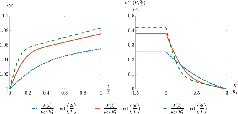
Figure 9: Solution to the force-control problem described in Example 3.5 with $\displaystyle F(t)=\mu_{0}\pi R_{1}^{2}\,\mathrm{erf}\left(\frac{At}{T}\right)$, where $A\in\{2,5,8\}$. The function $\lambda(t)$ reported here is the solution to the integral equation (3.61). The variation of the axial stress $\sigma^{zz}$ with $R$ at $t=\frac{T}{2}$ is shown.

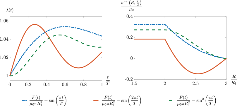
Figure 10: Solution to the force-control problem described in Example 3.5. The function $\lambda(t)$ reported here is the solution to the integral equation (3.61) with $F(t)=\mu_{0}\pi R_{1}^{2}\sin^{m}\left(\frac{\omega t}{T}\right)$, where $m\in\{1,2\}$ and $\omega\in\{\pi,2\pi\}$. Further, the variation of the axial stress $\sigma^{zz}$ with $R$ at $t=\frac{T}{2}$ is shown.

3.7 Residual stress

We assume that the body is unloaded after the accretion and ablation processes end. Let $T<t_{\text{ablation}}$. For $t>T$, $\lambda(t)=1$, and $F(t)=0$. The material metric of the resulting body has the following representation

$$\mathbf{G}=\begin{cases}\;\begin{bmatrix}1&0&0\\ 0&R^{2}&0\\ 0&0&1\end{bmatrix}\,,&\quad S_{1}(T)\leq R<R_{2}\,,\\ \begin{bmatrix}1&0&0\\ 0&\accentset{+}{r}^{2}(R)&0\\ 0&0&\accentset{+}{\lambda}^{4}(R)\end{bmatrix}\,,&\quad R_{2}\leq R\leq S_{2}(T)\,,\end{cases}$$ (3.64)

wherein the case $R<R_{2}$ is present only if $T<\accentset{-}{\tau}(R_{2})$. Let $\tilde{\varphi}:\mathcal{B}_{T}\rightarrow\mathcal{S}$ map the material manifold to the residually-stressed configuration. Let us consider the map $\tilde{\varphi}(R,\Theta,Z)=(\tilde{r},\tilde{\theta},\tilde{z})$ with $\tilde{r}=\tilde{r}(R)$, $\tilde{\theta}=\Theta$ and $\tilde{z}=\tilde{\lambda}^{2}Z$. Incompressibilty constraint can be expressed as

$$\begin{dcases}\frac{\tilde{\lambda}^{2}\tilde{r}(R)\tilde{r}^{\prime}(R)}{R}=1\,,&R\leq R_{2}\,,\\ \frac{\tilde{\lambda}^{2}\tilde{r}(R)\tilde{r}^{\prime}(R)}{\accentset{+}{\lambda}^{2}(R)\,\accentset{+}{r}(R)}=1\,,&R_{2}\leq R\,,\end{dcases}$$ (3.65)

which implies that

$$\tilde{r}^{2}(R)=\begin{cases}\displaystyle\tilde{r}^{2}(S_{1}(T))+\frac{R^{2}-S_{1}^{2}(T)}{\tilde{\lambda}^{2}}\,,&R\leq R_{2}\,,\\[10.0pt] \displaystyle\tilde{r}^{2}(S_{2}(T))-\frac{2}{\tilde{\lambda}^{2}}\int_{R}^{S_{2}(T)}\accentset{+}{\lambda}^{2}(\xi)\accentset{+}{r}(\xi)\text{d}\xi\,,&R_{2}\leq R\,.\end{cases}$$ (3.66)

The continuity of $\tilde{r}(R)$ at $R_{2}$ requires that

$$\tilde{r}^{2}(S_{2}(T))-\tilde{r}^{2}(S_{1}(T))=\frac{1}{\tilde{\lambda}^{2}}\left[R_{2}^{2}-S_{1}^{2}(T)+2\int_{R_{2}}^{S_{2}(T)}\accentset{+}{\lambda}^{2}(\xi)\accentset{+}{r}(\xi)\text{d}\xi\right]\,.$$ (3.67)

Observe that the knowledge of either $\tilde{r}(S_{1}(T))$ or $\tilde{r}(S_{2}(T))$ is sufficient to calculate $\tilde{r}(R)$. Let us take $\tilde{r}(S_{1}(T))$ as the only independent variable (other than $\tilde{\lambda}$), in terms of which

$$\tilde{r}^{2}(R)=\begin{cases}\displaystyle\tilde{r}^{2}(S_{1}(T))+\frac{R^{2}-S_{1}^{2}(T)}{\tilde{\lambda}^{2}}\,,&R\leq R_{2}\,,\\[10.0pt] \displaystyle\tilde{r}^{2}(S_{1}(T))+\frac{1}{\tilde{\lambda}^{2}}\left[R_{2}^{2}-S_{1}^{2}(T)+2\int_{R_{2}}^{R}\accentset{+}{\lambda}^{2}(\xi)\accentset{+}{r}(\xi)\text{d}\xi\right]\,,&R_{2}\leq R\,.\end{cases}$$ (3.68)

The deformation gradient reads

$$\tilde{\mathbf{F}}(R)=\begin{bmatrix}\tilde{r}^{\prime}(R)&0&0\\ 0&1&0\\ 0&0&\tilde{\lambda}^{2}\end{bmatrix}\,.$$ (3.69)

For $R\leq R_{2}$:

$$\mathbf{b}^{\sharp}(R)=\begin{bmatrix}[\tilde{r}^{\prime}(R)]^{2}&0&0\\ 0&\displaystyle\frac{1}{R^{2}}&0\\ 0&0&\tilde{\lambda}^{4}\\ \end{bmatrix}\,,\qquad\mathbf{c}^{\sharp}(R)=\begin{bmatrix}\displaystyle\frac{1}{[\tilde{r}^{\prime}(R)]^{2}}&0&0\\ 0&\displaystyle\frac{R^{2}}{\tilde{r}^{4}(R)}&0\\ 0&0&\displaystyle\frac{1}{\tilde{\lambda}^{4}}\\ \end{bmatrix}\,.$$ (3.70)

The principal invariants of $\mathbf{b}$ read

$$I_{1}(R)=[\tilde{r}^{\prime}(R)]^{2}+\frac{\tilde{r}^{2}(R)}{R^{2}}+\tilde{\lambda}^{4}\,,\qquad I_{2}(R)=[\tilde{r}^{\prime}(R)]^{2}\,\tilde{\lambda}^{4}+\frac{[\tilde{r}^{\prime}(R)]^{2}\,\tilde{r}^{2}(R)}{R^{2}}+\frac{\tilde{r}^{2}(R)\,\tilde{\lambda}^{4}}{R^{2}}\,.$$ (3.71)

Using (3.65)₁, the nonzero physical components of the residual Cauchy stress can be expressed as

$$\tilde{\sigma}^{rr}(R) =-p(R)+\frac{\alpha(R)\,R^{2}}{\tilde{\lambda}^{4}\tilde{r}^{2}(R)}-\frac{\beta(R)\tilde{\lambda}^{4}\tilde{r}^{2}(R)}{R^{2}}\,,$$ (3.72)

$$\hat{\tilde{\sigma}}^{\theta\theta}(R) =-p(R)+\frac{\alpha(R)\tilde{r}^{2}(R)}{R^{2}}-\frac{\beta(R)\,R^{2}}{\tilde{r}^{2}(R)}\,,$$

$$\tilde{\sigma}^{zz}(R) =-p(R)+\alpha(R)\,\tilde{\lambda}^{4}-\,\frac{\beta(R)}{\tilde{\lambda}^{4}}\,.$$

For $R<R_{2}$, the radial equilibrium equation and the traction boundary condition $\tilde{\sigma}^{rr}(S_{1}(T))=0$ imply that

$$\tilde{\sigma}^{rr}(R)= \int_{S_{1}(T)}^{R}\left[\frac{\alpha(\xi)}{\tilde{\lambda}^{4}}+\beta(\xi)\right]\left[\frac{\tilde{\lambda}^{2}}{\xi}-\frac{\xi^{3}}{\tilde{\lambda}^{2}\,\tilde{r}^{4}(\xi)}\right]d\xi\,,$$ (3.73)

$$\hat{\tilde{\sigma}}^{\theta\theta}(R)= \left[\frac{\alpha(R)}{\tilde{\lambda}^{4}}+\beta(R)\right]\left[\frac{\tilde{\lambda}^{4}\tilde{r}^{2}(R)}{R^{2}}-\frac{R^{2}}{\tilde{r}^{2}(R)}\right]+\tilde{\sigma}^{rr}(R)\,,$$

$$\tilde{\sigma}^{zz}(R)= \alpha(R)\left[\tilde{\lambda}^{4}-\frac{R^{2}}{\tilde{\lambda}^{4}\tilde{r}^{2}(R)}\right]+\beta(R)\left[\frac{\tilde{\lambda}^{4}\tilde{r}^{2}(R)}{R^{2}}-\frac{1}{\tilde{\lambda}^{4}}\right]+\tilde{\sigma}^{rr}(R)\,.$$

Now for $R\geq R_{2}$:

$$\mathbf{b}^{\sharp}(R)=\begin{bmatrix}\displaystyle[\tilde{r}^{\prime}(R)]^{2}&0&0\\ 0&\displaystyle\frac{1}{\accentset{+}{r}^{2}(R)}&0\\ 0&0&\displaystyle\frac{\tilde{\lambda}^{4}}{\accentset{+}{\lambda}^{4}(R)}\\ \end{bmatrix}\,,\qquad\mathbf{c}^{\sharp}(R)=\begin{bmatrix}\displaystyle\frac{1}{[\tilde{r}^{\prime}(R)]^{2}}&0&0\\ 0&\displaystyle\frac{\accentset{+}{r}^{2}(R)}{\tilde{r}^{4}(R)}&0\\ 0&0&\displaystyle\frac{\accentset{+}{\lambda}^{4}(R)}{\tilde{\lambda}^{4}}\\ \end{bmatrix}\,.$$ (3.74)

The principal invariants of $\mathbf{b}$ read

$$I_{1}(R)=[\tilde{r}^{\prime}(R)]^{2}+\frac{\tilde{r}^{2}(R)}{\accentset{+}{r}^{2}(R)}+\frac{\tilde{\lambda}^{4}}{\accentset{+}{\lambda}^{4}(R)}\,,\qquad I_{2}(R)=\frac{[\tilde{r}^{\prime}(R)]^{2}\,\tilde{r}^{2}(R)}{\accentset{+}{r}^{2}(R)}+\frac{\tilde{\lambda}^{4}\tilde{r}^{2}(R)}{\accentset{+}{r}^{2}(R)\accentset{+}{\lambda}^{4}(R)}+\frac{\tilde{\lambda}^{4}[\tilde{r}^{\prime}(R)]^{2}}{\accentset{+}{\lambda}^{4}(R)}\,.$$ (3.75)

Using (3.65)₂, the nonzero physical components of the residual Cauchy stress can be expressed as

$$\tilde{\sigma}^{rr}(R) =-p(R)+\alpha(R,t)\tilde{r}_{,R}^{2}(R)-\frac{\beta(R)}{\tilde{r}_{,R}^{2}(R)}\,,$$ (3.76)

$$\hat{\tilde{\sigma}}^{\theta\theta}(R) =-p(R)+\frac{\alpha(R)\tilde{r}^{2}(R)}{\accentset{+}{r}^{2}(R)}-\frac{\beta(R)\,\accentset{+}{r}^{2}(R)}{\tilde{r}^{2}(R)}\,,$$

$$\tilde{\sigma}^{zz}(R) =-p(R)+\frac{\alpha(R)\,\tilde{\lambda}^{4}}{\accentset{+}{\lambda}^{4}(R)}-\frac{\beta(R)\,\accentset{+}{\lambda}^{4}(R)}{\tilde{\lambda}^{4}}\,.$$

For $R\geq R_{2}$, the radial equilibrium equation and the traction boundary condition $\tilde{\sigma}^{rr}(S_{2}(T))=0$ give us

$$\tilde{\sigma}^{rr}(R)= -\int_{R}^{S_{2}(T)}\accentset{+}{\lambda}^{2}(\xi)\left[\frac{\alpha(\xi)}{\tilde{\lambda}^{4}}+\frac{\beta(\xi)}{\accentset{+}{\lambda}^{4}(\xi)}\right]\left[\frac{\tilde{\lambda}^{2}}{\accentset{+}{r}(\xi)}-\frac{\accentset{+}{r}^{3}(\xi)\accentset{+}{\lambda}^{4}(\xi)}{\tilde{\lambda}^{2}\,\tilde{r}^{4}(\xi)}\right]d\xi\,,$$ (3.77)

$$\hat{\tilde{\sigma}}^{\theta\theta}(R)= \left[\frac{\alpha(R)}{\tilde{\lambda}^{4}}+\frac{\beta(R)}{\accentset{+}{\lambda}^{4}(R)}\right]\left[\frac{\tilde{\lambda}^{4}\tilde{r}^{2}(R)}{\accentset{+}{r}^{2}(R)}-\frac{\accentset{+}{r}^{2}(R)\accentset{+}{\lambda}^{4}(R)}{\tilde{r}^{2}(R)}\right]+\tilde{\sigma}^{rr}(R),$$

$$\tilde{\sigma}^{zz}(R)= \alpha(R)\left[\frac{\tilde{\lambda}^{4}}{\accentset{+}{\lambda}^{4}(R)}-\frac{\accentset{+}{\lambda}^{4}(R)\accentset{+}{r}^{2}(R)}{\tilde{\lambda}^{4}\tilde{r}^{2}(R)}\right]+\beta(R)\left[\frac{\tilde{\lambda}^{4}\tilde{r}^{2}(R)}{\accentset{+}{\lambda}^{4}(R)\accentset{+}{r}^{2}(R)}-\frac{\accentset{+}{\lambda}^{4}(R)}{\tilde{\lambda}^{4}}\right]+\tilde{\sigma}^{rr}(R).$$

The continuity of $\tilde{\sigma}^{rr}(R)$ at $R_{2}$ requires that

$$\tilde{\Upsilon}:=\int_{S_{1}(T)}^{R_{2}}\left[\frac{\alpha(\xi)}{\tilde{\lambda}^{4}}+\beta(\xi)\right]\left[\frac{\tilde{\lambda}^{2}}{\xi}-\frac{\xi^{3}}{\tilde{\lambda}^{2}\,\tilde{r}^{4}(\xi)}\right]d\xi+\int_{R_{2}}^{S_{2}(T)}\accentset{+}{\lambda}^{2}(\xi)\left[\frac{\alpha(\xi)}{\tilde{\lambda}^{4}}+\frac{\beta(\xi)}{\accentset{+}{\lambda}^{4}(\xi)}\right]\left[\frac{\tilde{\lambda}^{2}}{\accentset{+}{r}(\xi)}-\frac{\accentset{+}{r}^{3}(\xi)\accentset{+}{\lambda}^{4}(\xi)}{\tilde{\lambda}^{2}\,\tilde{r}^{4}(\xi)}\right]d\xi=0\,.$$ (3.79)

Absence of an axial force in the residually-stressed state implies that

$$\int_{S_{1}(T)}^{S_{2}(T)}2\pi R\,\tilde{P}^{zZ}(R)\text{d}R=0\,,$$ (3.80)

where $\tilde{P}^{zZ}(R)=\displaystyle\frac{\tilde{\sigma}^{zz}(R)}{\tilde{\lambda}^{2}}$ is the $zZ$- component of the residual Piola-Kirchhoff stress, calculated as

$$\tilde{P}^{zZ}(R)=\begin{cases}\alpha(R)\left[\tilde{\lambda}^{2}-\frac{R^{2}}{\tilde{\lambda}^{6}\tilde{r}^{2}(R)}\right]+\beta(R)\left[\frac{\tilde{\lambda}^{2}\tilde{r}^{2}(R)}{R^{2}}-\frac{1}{\tilde{\lambda}^{6}}\right]+\frac{\tilde{\sigma}^{rr}(R)}{\tilde{\lambda}^{2}}\,,&R\leq R_{2}\,,\\[10.0pt] \alpha(R)\left[\frac{\tilde{\lambda}^{2}}{\accentset{+}{\lambda}^{4}(R)}-\frac{\accentset{+}{\lambda}^{4}(R)\accentset{+}{r}^{2}(R)}{\tilde{\lambda}^{6}\tilde{r}^{2}(R)}\right]+\beta(R)\left[\frac{\tilde{\lambda}^{2}\tilde{r}^{2}(R)}{\accentset{+}{\lambda}^{4}(R)\accentset{+}{r}^{2}(R)}-\frac{\accentset{+}{\lambda}^{4}(R)}{\tilde{\lambda}^{6}}\right]+\frac{\tilde{\sigma}^{rr}(R)}{\tilde{\lambda}^{2}}\,,&R_{2}\leq R\,.\end{cases}$$ (3.81)

Residual stress in the case of a neo-Hookean solid.

Consider a homogeneous neo-Hookean material for which $\alpha(R)={\mu}(R)=\mu_{0}>0$ and $\beta(R)=0$ as in the previous section. The nonzero components of the residual Cauchy stress are written as

$$\tilde{\sigma}^{rr}(R) =\begin{dcases}\frac{\mu_{0}}{\tilde{\lambda}^{2}}\int_{S_{1}(T)}^{R}\frac{\text{d}\xi}{\xi}-\frac{\mu_{0}}{\tilde{\lambda}^{6}}\int_{S_{1}(T)}^{R}\frac{\xi^{3}\text{d}\xi}{\tilde{r}^{4}(\xi)}\,,&R<R_{2}\,,\\ -\frac{\mu_{0}}{\tilde{\lambda}^{2}}\int_{R}^{S_{2}(T)}\frac{\accentset{+}{\lambda}^{2}(\xi)d\xi}{\accentset{+}{r}(\xi)}+\frac{\mu_{0}}{\tilde{\lambda}^{6}}\int_{R}^{S_{2}(T)}\frac{\accentset{+}{r}^{3}(\xi)\accentset{+}{\lambda}^{6}(\xi)d\xi}{\tilde{r}^{4}(\xi)}\,,&R\geq R_{2}\,,\end{dcases}$$ (3.82)

$$\hat{\tilde{\sigma}}^{\theta\theta}(R) =\begin{dcases}\mu_{0}\left[\frac{\tilde{r}^{2}(R)}{R^{2}}-\frac{R^{2}}{\tilde{\lambda}^{4}\,\tilde{r}^{2}(R)}\right]+\tilde{\sigma}^{rr}(R)\,,&R<R_{2}\,,\\ \mu_{0}\left[\frac{\tilde{r}^{2}(R)}{\accentset{+}{r}^{2}(R)}-\frac{\accentset{+}{\lambda}^{4}(R)\accentset{+}{r}^{2}(R)}{\tilde{\lambda}^{4}\tilde{r}^{2}(R)}\right]+\tilde{\sigma}^{rr}(R)\,,&R\geq R_{2}\,,\end{dcases}$$

$$\tilde{\sigma}^{zz}(R) =\begin{dcases}\mu_{0}\left[\tilde{\lambda}^{4}-\frac{R^{2}}{\tilde{\lambda}^{4}\tilde{r}^{2}(R)}\right]+\tilde{\sigma}^{rr}(R)\,,&R<R_{2}\,,\\ \mu_{0}\left[\frac{\tilde{\lambda}^{4}}{\accentset{+}{\lambda}^{4}(R)}-\frac{\accentset{+}{\lambda}^{4}(R)\accentset{+}{r}^{2}(R)}{\tilde{\lambda}^{4}\tilde{r}^{2}(R)}\right]+\tilde{\sigma}^{rr}(R)\,,&R\geq R_{2}\,.\end{dcases}$$

Continuity of $\tilde{\sigma}^{rr}$, i.e., (3.79) simplifies to read

$$\tilde{\lambda}^{4}\left[\log\left({\frac{R_{2}}{S_{1}(T)}}\right)+\int_{R_{2}}^{S_{2}(T)}\frac{\accentset{+}{\lambda}^{2}(\xi)d\xi}{\accentset{+}{r}(\xi)}\right]-\left[\int_{S_{1}(T)}^{R_{2}}\frac{\xi^{3}d\xi}{\tilde{r}^{4}(\xi)}+\int_{R_{2}}^{S_{2}(T)}\frac{\accentset{+}{r}^{3}(\xi)\accentset{+}{\lambda}^{6}(\xi)d\xi}{\tilde{r}^{4}(\xi)}\right]=0\,.$$ (3.83)

Further,

$$\tilde{P}^{zZ}(R)=\begin{cases}\mu_{0}\left[\tilde{\lambda}^{2}-\frac{R^{2}}{\tilde{\lambda}^{6}\tilde{r}^{2}(R)}\right]+\frac{\tilde{\sigma}^{rr}(R)}{\tilde{\lambda}^{2}}\,,&R\leq R_{2}\,,\\[10.0pt] \mu_{0}\left[\frac{\tilde{\lambda}^{2}}{\accentset{+}{\lambda}^{4}(R)}-\frac{\accentset{+}{\lambda}^{4}(R)\accentset{+}{r}^{2}(R)}{\tilde{\lambda}^{6}\tilde{r}^{2}(R)}\right]+\frac{\tilde{\sigma}^{rr}(R)}{\tilde{\lambda}^{2}}\,,&R_{2}\leq R\,,\end{cases}$$ (3.84)

so that the zero axial force condition (3.80) implies that

$$\mu_{0}\int_{S_{1}(T)}^{R_{2}}\left[\tilde{\lambda}^{2}-\frac{R^{2}}{\tilde{\lambda}^{6}\tilde{r}^{2}(R)}\right]R\,\text{d}R+\mu_{0}\int_{R_{2}}^{S_{2}(T)}\left[\frac{\tilde{\lambda}^{2}}{\accentset{+}{\lambda}^{4}(R)}-\frac{\accentset{+}{\lambda}^{4}(R)\accentset{+}{r}^{2}(R)}{\tilde{\lambda}^{6}\tilde{r}^{2}(R)}\right]R\,\text{d}R+\frac{1}{\tilde{\lambda}^{2}}\int_{S_{1}(T)}^{S_{2}(T)}R\,\tilde{\sigma}^{rr}(R)\,\text{d}R=0\,.$$ (3.85)

Note that

$$\int_{S_{1}(T)}^{S_{2}(T)}R\,\tilde{\sigma}^{rr}(R)\,\text{d}R =\frac{\mu_{0}}{\tilde{\lambda}^{2}}\int_{S_{1}(T)}^{R_{2}}\left[\int_{S_{1}(T)}^{R}\frac{\text{d}\xi}{\xi}\right]R\,\text{d}R-\frac{\mu_{0}}{\tilde{\lambda}^{6}}\int_{S_{1}(T)}^{R_{2}}\left[\int_{S_{1}(T)}^{R}\frac{\xi^{3}\text{d}\xi}{\tilde{r}^{4}(\xi)}\right]R\,\text{d}R$$ (3.86)

$$\quad-\frac{\mu_{0}}{\tilde{\lambda}^{2}}\int_{R_{2}}^{S_{2}(T)}\left[\int_{R}^{S_{2}(T)}\frac{\accentset{+}{\lambda}^{2}(\xi)d\xi}{\accentset{+}{r}(\xi)}\right]R\,\text{d}R$$

$$\quad+\frac{\mu_{0}}{\tilde{\lambda}^{6}}\int_{R_{2}}^{S_{2}(T)}\left[\int_{R}^{S_{2}(T)}\frac{\accentset{+}{r}^{3}(\xi)\accentset{+}{\lambda}^{6}(\xi)d\xi}{\tilde{r}^{4}(\xi)}\right]R\,\text{d}R\,,$$

or equivalently,

$$\int_{S_{1}(T)}^{S_{2}(T)}R\,\tilde{\sigma}^{rr}(R)\,\text{d}R =\frac{\mu_{0}}{2\tilde{\lambda}^{2}}\left[R_{2}^{2}\log\left(\frac{R_{2}}{S_{2}(T)}\right)-\frac{R_{2}^{2}-S_{1}^{2}(T)}{2}\right]-\frac{\mu_{0}}{2\tilde{\lambda}^{6}}\int_{S_{1}(T)}^{R}\frac{\left[R_{2}^{2}-\xi^{2}\right]\xi^{3}\text{d}\xi}{\tilde{r}^{4}(\xi)}$$ (3.87)

$$\quad-\frac{\mu_{0}}{2\tilde{\lambda}^{2}}\int_{R_{2}}^{S_{2}(T)}\frac{\left[\xi^{2}-R_{2}^{2}\right]\accentset{+}{\lambda}^{2}(\xi)\,d\xi}{\accentset{+}{r}(\xi)}+\frac{\mu_{0}}{2\tilde{\lambda}^{6}}\int_{R_{2}}^{S_{2}(T)}\frac{\left[\xi^{2}-R_{2}^{2}\right]\accentset{+}{r}^{3}(\xi)\accentset{+}{\lambda}^{6}(\xi)d\xi}{\tilde{r}^{4}(\xi)}\,.$$

This in view of (3.83) implies that

$$\int_{S_{1}(T)}^{S_{2}(T)}R\,\tilde{\sigma}^{rr}(R)\,\text{d}R= -\frac{\mu_{0}[R_{2}^{2}-S_{1}^{2}(T)]}{4\tilde{\lambda}^{2}}+\frac{\mu_{0}}{2\tilde{\lambda}^{6}}\int_{S_{1}(T)}^{R}\frac{\xi^{5}\text{d}\xi}{\tilde{r}^{4}(\xi)}$$ (3.88)

$$-\frac{\mu_{0}}{2\tilde{\lambda}^{2}}\int_{R_{2}}^{S_{2}(T)}\frac{\xi^{2}\accentset{+}{\lambda}^{2}(\xi)\,d\xi}{\accentset{+}{r}(\xi)}+\frac{\mu_{0}}{2\tilde{\lambda}^{6}}\int_{R_{2}}^{S_{2}(T)}\frac{\xi^{2}\accentset{+}{r}^{3}(\xi)\accentset{+}{\lambda}^{6}(\xi)d\xi}{\tilde{r}^{4}(\xi)}\,.$$

Thus, (3.85) can be rewritten as

$$\tilde{\lambda}^{2}\left[\frac{R_{2}^{2}-S_{1}^{2}(T)}{2}+\int_{R_{2}}^{S_{2}(T)}\frac{R\,\text{d}R}{\accentset{+}{\lambda}^{4}(R)}\right]-\frac{1}{\tilde{\lambda}^{6}}\left[\int_{S_{1}(T)}^{R_{2}}\frac{R^{3}\,\text{d}R}{\tilde{r}^{2}(R)}+\int_{R_{2}}^{S_{2}(T)}\frac{R\,\accentset{+}{\lambda}^{4}(R)\accentset{+}{r}^{2}(R)\,\text{d}R}{\tilde{r}^{2}(R)}\right]$$ (3.89)

$$-\frac{1}{2\tilde{\lambda}^{4}}\left[\frac{R_{2}^{2}-S_{1}^{2}(T)}{2}+\int_{R_{2}}^{S_{2}(T)}\frac{\xi^{2}\accentset{+}{\lambda}^{2}(\xi)\,d\xi}{\accentset{+}{r}(\xi)}\right]+\frac{1}{2\tilde{\lambda}^{8}}\left[\int_{S_{1}(T)}^{R_{2}}\frac{\xi^{5}d\xi}{\,\tilde{r}^{4}(\xi)}+\int_{R_{2}}^{S_{2}(T)}\frac{\xi^{2}\accentset{+}{r}^{3}(\xi)\accentset{+}{\lambda}^{6}(\xi)\,d\xi}{\tilde{r}^{4}(\xi)}\right]=0\,.$$

Determining the residual stretch and stress requires calculating the unknowns $\tilde{r}(S_{1}(T))$ and $\tilde{\lambda}$ that satisfy (3.83) and (3.89).

Remark 3.6.

The functions $\accentset{+}{\lambda}(R)$ and $\accentset{+}{r}(R)$ are known from the deformation history of the bar prior to the removal of external loads, and hence, are treated as given quantities while solving for the residually-stressed state. Observe that

$$\tilde{r}(R)=\begin{cases}\displaystyle\frac{R}{\tilde{\lambda}}\,,&R\leq R_{2}\,,\\[10.0pt] \displaystyle\frac{\accentset{+}{\lambda}(R)\accentset{+}{r}(R)}{\tilde{\lambda}}\,,&R_{2}\leq R\,,\end{cases}$$ (3.90)

is a solution that satisfies (3.65), (3.83) and (3.89). The residual Cauchy stress components $\tilde{\sigma}^{rr}$ and $\hat{\tilde{\sigma}}^{\theta\theta}$ vanish for this solution. Moreover,

$$\tilde{P}^{zZ}(R)=\begin{cases}\displaystyle\mu_{0}\left[\tilde{\lambda}^{2}-\frac{1}{\tilde{\lambda}^{4}}\right]\,,&R\leq R_{2}\,,\\[10.0pt] \displaystyle\mu_{0}\left[\frac{\tilde{\lambda}^{2}}{\accentset{+}{\lambda}^{4}(R)}-\frac{\accentset{+}{\lambda}^{2}(R)}{\tilde{\lambda}^{4}}\right]\,,&R_{2}\leq R\,,\end{cases}$$ (3.91)

so that the zero axial force condition (3.80) requires that

$$\int_{S_{1}(T)}^{R_{2}}\mu_{0}R\left[\tilde{\lambda}^{2}-\frac{1}{\tilde{\lambda}^{4}}\right]\text{d}R+\int_{R_{2}}^{S_{2}(T)}\mu_{0}R\left[\frac{\tilde{\lambda}^{2}}{\accentset{+}{\lambda}^{4}(R)}-\frac{\accentset{+}{\lambda}^{2}(R)}{\tilde{\lambda}^{4}}\right]\text{d}R=0\,.$$ (3.92)

This implies that

$$\tilde{\lambda}^{6}=\displaystyle\frac{R_{2}^{2}-S_{1}^{2}(T)+2\displaystyle\int_{R_{2}}^{S_{2}(T)}R\,\accentset{+}{\lambda}^{2}(R)\text{d}R}{R_{2}^{2}-S_{1}^{2}(T)+2\displaystyle\int_{R_{2}}^{S_{2}(T)}\frac{R\,\text{d}R}{\accentset{+}{\lambda}^{4}(R)}}\,.$$ (3.93)

Example 3.7.

Consider a displacement-control problem with $R_{2}=2R_{1}\,$, $\accentset{-}{\upsilon}=\frac{R_{1}}{2T}$, $\accentset{+}{\upsilon}=\frac{R_{1}}{T}$, and $\lambda(t)=1+a\left(\frac{t}{T}\right)^{n}$, where $n\geq 0$, and $a\in\mathbb{R}$. Then $t_{\text{ablation}}=2T>T$, $S_{1}(T)=1.5R_{1}$ and $S_{2}(T)=3R_{1}$. First we need to find $\accentset{+}{r}:[R_{2},S_{2}(T)]\rightarrow\mathbb{R}$ as in Example 3.4. With the knowledge of $\accentset{+}{\lambda}$ and $\accentset{+}{r}$ (see Fig. 11), we need to find $\tilde{r}(S_{1}(T))$ and $\tilde{\lambda}$ that satisfy the following nonlinear integral equations

$$\begin{cases}\displaystyle\tilde{\lambda}^{2}\left[\frac{R_{2}^{2}-S_{1}^{2}(T)}{2}+\int_{R_{2}}^{S_{2}(T)}\frac{R\,\text{d}R}{\accentset{+}{\lambda}^{4}(R)}\right]-\frac{1}{\tilde{\lambda}^{6}}\left[\int_{S_{1}(T)}^{R_{2}}\frac{R^{3}\,\text{d}R}{\tilde{r}^{2}(R)}+\int_{R_{2}}^{S_{2}(T)}\frac{R\,\accentset{+}{\lambda}^{4}(R)\accentset{+}{r}^{2}(R)\,\text{d}R}{\tilde{r}^{2}(R)}\right]\\[8.0pt] \displaystyle\qquad-\frac{1}{2\tilde{\lambda}^{4}}\left[\frac{R_{2}^{2}-S_{1}^{2}(T)}{2}+\int_{R_{2}}^{S_{2}(T)}\frac{\xi^{2}\accentset{+}{\lambda}^{2}(\xi)\,d\xi}{\accentset{+}{r}(\xi)}\right]+\frac{1}{2\tilde{\lambda}^{8}}\left[\int_{S_{1}(T)}^{R_{2}}\frac{\xi^{5}d\xi}{\,\tilde{r}^{4}(\xi)}+\int_{R_{2}}^{S_{2}(T)}\frac{\xi^{2}\accentset{+}{r}^{3}(\xi)\accentset{+}{\lambda}^{6}(\xi)\,d\xi}{\tilde{r}^{4}(\xi)}\right]=0\,,\\[20.0pt] \displaystyle\tilde{\lambda}^{4}\left[\log\left({\frac{R_{2}}{S_{1}(T)}}\right)+\int_{R_{2}}^{S_{2}(T)}\frac{\accentset{+}{\lambda}^{2}(\xi)d\xi}{\accentset{+}{r}(\xi)}\right]-\left[\int_{S_{1}(T)}^{R_{2}}\frac{\xi^{3}d\xi}{\tilde{r}^{4}(\xi)}+\int_{R_{2}}^{S_{2}(T)}\frac{\accentset{+}{r}^{3}(\xi)\accentset{+}{\lambda}^{6}(\xi)d\xi}{\tilde{r}^{4}(\xi)}\right]=0\,,\end{cases}$$ (3.94)

where

$$\tilde{r}^{2}(R)=\begin{cases}\displaystyle\tilde{r}^{2}(S_{1}(T))+\frac{R^{2}-S_{1}^{2}(T)}{\tilde{\lambda}^{2}}\,,&R\leq R_{2}\,,\\[10.0pt] \displaystyle\tilde{r}^{2}(S_{1}(T))+\frac{1}{\tilde{\lambda}^{2}}\left[R_{2}^{2}-S_{1}^{2}(T)+2\int_{R_{2}}^{R}\accentset{+}{\lambda}^{2}(\xi)\accentset{+}{r}(\xi)\text{d}\xi\right]\,,&R_{2}\leq R\,.\end{cases}$$ (3.95)

We solve this system numerically in Matlab for $a\in\big{\{}\pm\frac{1}{2}\big{\}}$ and $n\in\big{\{}\frac{1}{2},1,2\big{\}}$ (with the numerical values $R_{1}=1$ and $T=1$). Since the numerical values of $\tilde{\sigma}^{rr}(R)$ and $\tilde{\sigma}^{\theta\theta}(R)$ are negligible, they are not reported here. The values of $\tilde{\lambda}^{2}$ (see Table 1) and $\tilde{\sigma}^{zz}$ (see Fig. 12) obtained numerically agree with those described in Remark 3.6. From Fig. 12, we observe that even if a bar is subjected only to elongation, the residual axial stresses in the initial portion of the final body are compressive due to stress redistribution after the bar is set free. Similarly, tensile residual axial stress is observed in the initial portion of a bar shortened during accretion-ablation.

	$n=\frac{1}{2}$	$n=1$	$n=2$
$a=\frac{1}{2}$	$1.4733$	$1.3547$	$1.2349$
$a=-\frac{1}{2}$	$0.4727$	$0.5514$	$0.6477$

Table 1: Residual stretch $\tilde{\lambda}^{2}$ in the body when it is set free after the displacement-control loading described in Example 3.7.

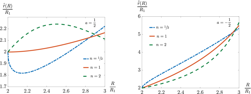
Figure 11: Solution of the displacement-control problem described in Example 3.7 during the loading process.

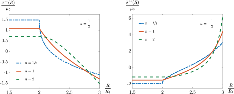
Figure 12: Residual stress $\tilde{\sigma}^{zz}(R)$ in the body (Example 3.7) after the removal of the external forces for the displacement-control loading $\lambda(t)=1+a\left(\frac{t}{T}\right)^{n}$, where $a\in\left\{\pm\frac{1}{2}\right\}$ and $n\in\left\{\frac{1}{2},1,2\right\}$.

Example 3.8.

Consider a force-control problem with $R_{2}=2R_{1}$, $\accentset{-}{\upsilon}=\frac{R_{1}}{2T}$, and $\accentset{+}{\upsilon}=\frac{R_{1}}{T}$. Then $t_{\text{ablation}}=2T>T$, $S_{1}(T)=1.5R_{1}$, and $S_{2}(T)=3R_{1}$. First we find the functions $\lambda(t)$ and $\accentset{+}{r}(R)$ as in Example 3.5, which are then used to solve (3.94) and (3.95) for $\tilde{r}(S_{1}(T))$ and $\tilde{\lambda}$. Assume the numerical values $R_{1}=1$ and $T=1$. We report $\tilde{\sigma}^{zz}$ as a function of $R$ in the residually-stressed configuration taking $F(t)$ as polynomial (Fig. 13), error (Fig. 14), and sinusoidal (Fig. 15) functions of time $t$. The residual stretches $\tilde{\lambda}^{2}$ for the same choices of $F(t)$ are given in Table 2. In Fig. 13 we compare the axial residual stress for loads varying monotonically as linear and quadratic functions of time. A monotonically increasing tensile $F(t)$ induces a compressive $\tilde{\sigma}^{zz}$ in the initial portion of the body, although $\tilde{\lambda}^{2}>1$. Similarly, a monotonically increasing compressive $F(t)$ leaves a tensile $\tilde{\sigma}^{zz}$ in the initial portion of the final body along with a residual contraction $\tilde{\lambda}^{2}<1$. In Fig. 14, $\tilde{\sigma}^{zz}$ is observed to be almost the same towards the outermost accreted layers for all the three loading paths. This is probably because the load when those outermost layers were accreted was very close to the asympotic limit of $F(t)$ in all the three cases. As a result, all those layers experience the same state of stress during loading as well as when they are set free. In Fig. 15, we look at the residual stress print left after different sinusoidal loading cycles and observe that $\tilde{\sigma}^{zz}$ remains zero on the outer boundary even after the bar is unloaded.

$\displaystyle\frac{F(t)}{\mu_{0}\pi R_{1}^{2}}$		$\tilde{\lambda}^{2}$
$\text{erf}\left(\frac{At}{T}\right)$	$A=2$	$1.0603$
	$A=5$	$1.0835$
	$A=8$	$1.0910$
$a\left(\frac{t}{T}\right)^{n}$	$a=5$, $n=1$	$1.2158$
	$a=5$, $n=2$	$1.1166$
	$a=-5$, $n=1$	$0.8479$
	$a=-5$, $n=2$	$0.9051$
$\sin^{m}\left(\frac{\omega t}{T}\right)$	$m=1$, $\omega=\pi$	$1.0617$
	$m=1$, $\omega=2\pi$	$1.0219$
	$m=2$, $\omega=\pi$	$1.0468$

Table 2: Residual stretch $\tilde{\lambda}^{2}$ in the body when it is set free after the force-control loading described in Example 3.8.

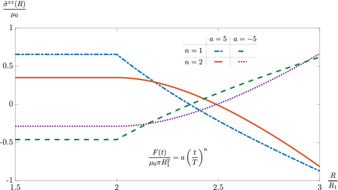
Figure 13: Residual stress $\tilde{\sigma}^{zz}(R)$ in the body (Example 3.8) when it is set free after the loading $F(t)=\pm 5\mu_{0}\pi R_{1}^{2}\left(\frac{t}{T}\right)^{n}$, where $n\in\{1,2\}$.

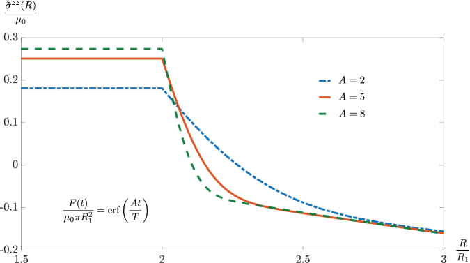
Figure 14: Residual stress $\tilde{\sigma}^{zz}(R)$ in the body (Example 3.8) when it is set free after the loading $F(t)=\mu_{0}\pi R_{1}^{2}\,\mathsf{erf}\left(\frac{At}{T}\right)$, where $A\in\{2,5,8\}$.

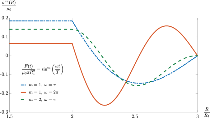
Figure 15: Residual stress $\tilde{\sigma}^{zz}(R)$ in the final body (Example 3.8). During the accretion-ablation process this body was under a sinusoidal axial force.

3.8 Response of a $3$D-printed bar under axial loads

Let us assume that $T_{1}$ and $T_{2}$ are such that $0<T<T_{1}<T_{2}$, and consider a $3$D-printed thick hollow cylinder in the time interval $[0,T_{2}]$. Accretion/ablation occurs during the interval $[0,T]$ under some time-dependent axial load, after which the body is in an unloaded state until $t=T_{1}$, and service loads are applied during $[T_{1},T_{2}]$. The motion map has the following representation

$$\varphi_{t}(R,\Theta,Z)=\begin{cases}\big{(}\,r(R,t),\Theta,\lambda^{2}(t)Z\,\big{)}\,,\quad&t\leq T\,,\\ \big{(}\,\tilde{r}(R),\Theta,\tilde{\lambda}^{2}Z\,\big{)}\,,\quad&T<t<T_{1}\,,\\ \big{(}\,r_{s}(R,t),\Theta,\lambda_{s}^{2}(t)\tilde{\lambda}^{2}Z\,\big{)}\,,\quad&T_{1}\leq t\leq T_{2}\,,\end{cases}$$ (3.96)

where $S_{1}(t)\leq R\leq S_{2}(t)$, and $\lambda_{s}^{2}(t)$ is the axial stretch due to the service load. The functions $\lambda$, $\lambda_{s}$ are assumed to satisfy the following conditions: $\lambda(0)=1$, $\lambda_{s}(T_{1})=1$. Further, notice that

$$S_{1}(t)=\begin{cases}R_{1}+\accentset{-}{\upsilon}t\,,\quad&t\leq T\,,\\ S_{1}(T)\,,\quad&t>T\end{cases}\;,\qquad S_{2}(t)=\begin{cases}R_{2}+\accentset{+}{\upsilon}t\,,\quad&t\leq T\,,\\ S_{2}(T)\,,\quad&t>T\,,\end{cases}$$ (3.97)

so that they are invertible only in $[0,T]$, with their inverses being $\accentset{-}{\tau}$ and $\accentset{+}{\tau}$, respectively. Axial force and the Cauchy stress are written as

$$F(t)=\begin{cases}\mu_{0}\pi R_{1}^{2}\;f_{l}(t)\,,\quad&t\leq T\,,\\ 0\,,\quad&T<t<T_{1}\,,\\ \mu_{0}\pi R_{1}^{2}\;f_{s}(t)\,,\quad&T_{1}\leq t\leq T_{2}\,,\end{cases}\qquad\bm{\sigma}(R,t)=\begin{cases}\bm{\sigma}_{l}(R,t)\,,\quad&t\leq T\,,\\ \tilde{\bm{\sigma}}(R)\,,\quad&T<t<T_{1}\,,\\ \bm{\sigma}_{s}(R,t)\,,\quad&T_{1}\leq t\leq T_{2}\,,\end{cases}$$ (3.98)

where the functions $f_{l}$, $f_{s}$ are the dimensionless axial forces during the acrretion-ablation process and service loading, respectively, and are assumed to satisfy the following conditions: $f_{l}(0)=0$, $f_{s}(T_{1})=0$. The $zz$-component of the Cauchy stress during service loading is written as

$$\sigma_{s}^{zz}(R,t)=\begin{cases}\displaystyle\lambda_{s}^{4}(t)\tilde{\lambda}^{4}-\frac{1}{\lambda_{s}^{2}(t)\tilde{\lambda}^{2}}\,,\quad&S_{1}(T)\leq R\leq R_{2}\,,\\[12.0pt] \displaystyle\frac{\lambda_{s}^{4}(t)\tilde{\lambda}^{4}}{\accentset{+}{\lambda}^{4}(R)}-\frac{\accentset{+}{\lambda}^{2}(R)}{\lambda_{s}^{2}(t)\tilde{\lambda}^{2}}\,,\quad&R_{2}\leq R\leq S_{2}(T)\,,\end{cases}$$ (3.99)

which implies that

$$\frac{F(t)}{2\pi\mu_{0}}=\frac{R_{2}^{2}-S_{1}^{2}(T)}{2}\left[\lambda_{s}^{2}(t)\tilde{\lambda}^{2}-\frac{1}{\lambda_{s}^{4}(t)\tilde{\lambda}^{4}}\right]+\lambda_{s}^{2}(t)\tilde{\lambda}^{2}\int_{R_{2}}^{S_{2}(T)}\frac{R\,\text{d}R}{\accentset{+}{\lambda}^{4}(R)}-\frac{1}{\lambda_{s}^{4}(t)\tilde{\lambda}^{4}}\int_{R_{2}}^{S_{2}(T)}R\accentset{+}{\lambda}^{2}(R)\text{d}R\,,$$ (3.100)

where $T_{1}\leq t\leq T_{2}$. This can be rearranged as

$$\frac{F(t)}{2\pi\mu_{0}}=\lambda_{s}^{2}(t)\tilde{\lambda}^{2}\left[\frac{R_{2}^{2}-S_{1}^{2}(T)}{2}+\int_{R_{2}}^{S_{2}(T)}\frac{R\,\text{d}R}{\accentset{+}{\lambda}^{4}(R)}\right]-\frac{1}{\lambda_{s}^{4}(t)\tilde{\lambda}^{4}}\left[\frac{R_{2}^{2}-S_{1}^{2}(T)}{2}+\int_{R_{2}}^{S_{2}(T)}R\accentset{+}{\lambda}^{2}(R)\text{d}R\right]\,,$$ (3.101)

with

$$\tilde{\lambda}^{6}=\frac{R_{2}^{2}-S_{1}^{2}(T)+2\int_{R_{2}}^{S_{2}(T)}R\accentset{+}{\lambda}^{2}(R)\text{d}R}{R_{2}^{2}-S_{1}^{2}(T)+2\int_{R_{2}}^{S_{2}(T)}\frac{R}{\accentset{+}{\lambda}^{4}(R)}\text{d}R}\,.$$ (3.102)

This implies the following force-stretch relationship

$$f_{s}(t)=a\left[\lambda_{s}^{2}(t)-\frac{1}{\lambda_{s}^{4}(t)}\right]\,,$$ (3.103)

where

$$a=\frac{1}{R_{1}^{2}}\left[R_{2}^{2}-S_{1}^{2}(T)+2\int_{R_{2}}^{S_{2}(T)}R\accentset{+}{\lambda}^{2}(R)\text{d}R\right]^{\frac{1}{3}}\left[R_{2}^{2}-S_{1}^{2}(T)+2\int_{R_{2}}^{S_{2}(T)}\frac{R}{\accentset{+}{\lambda}^{4}(R)}\text{d}R\right]^{\frac{2}{3}}\,.$$ (3.104)

A stress-free elastic body with the same size as the $3$D-printed body.

First observe that in the absence of accretion/ablation (i.e., $\accentset{+}{\upsilon}=\accentset{-}{\upsilon}=0$) Eq. (3.100) simplifies to read

$$\frac{F(t)}{2\pi\mu_{0}}=\frac{R_{2}^{2}-R_{1}^{2}}{2}\left[\lambda^{2}(t)-\frac{1}{\lambda^{4}(t)}\right]\,.$$ (3.105)

In this problem, we replace $R_{1}$ by $\tilde{r}(S_{1}(T))$, $R_{2}$ by $\tilde{r}(S_{2}(T))$, and $L$ by $\tilde{\lambda}^{2}L$. Consider a stress-free thick cylinder of inner radius $\tilde{r}(S_{1}(T))=\frac{S_{1}(T)}{\tilde{\lambda}}$, outer radius $\tilde{r}(S_{2}(T))=\frac{\lambda(T)s_{2}(T)}{\tilde{\lambda}}$, initial length $\tilde{\lambda}^{2}L$ and subject it to the same service load during the time interval $[T_{1},T_{2}]$. For this new problem, let the motion be denoted as

$$\accentset{\circ}{\varphi}_{t}(R,\Theta,Z)=\big{(}\,\accentset{\circ}{r}_{s}(R,t),\Theta,\accentset{\circ}{\lambda}_{s}^{2}(t)Z\,\big{)}\,,$$ (3.106)

where $\frac{S_{1}(T)}{\tilde{\lambda}}\leq R\leq\frac{\lambda(T)\,s_{2}(T)}{\tilde{\lambda}}$, and $0\leq Z\leq\tilde{\lambda}^{2}L$. Let the axial force be $F_{s}(t)=\mu_{0}\pi R_{1}^{2}\;f_{s}(t)$, and denote the Cauchy stress by $\accentset{\circ}{\bm{\sigma}}_{s}$. For $\tilde{r}(S_{1}(T))\leq\tilde{R}\leq\tilde{r}(S_{2}(T))$,

$$\accentset{\circ}{\sigma}_{s}^{zz}(\tilde{R},t)=\mu_{0}\left[\accentset{\circ}{\lambda}_{s}^{4}(t)-\frac{1}{\accentset{\circ}{\lambda}_{s}^{2}(t)}\right]\,,$$ (3.107)

which implies that the axial force can be expressed as

$$\frac{F_{s}(t)}{2\pi\mu_{0}}=\frac{\lambda^{2}(T)s_{2}^{2}(T)-S_{1}^{2}(T)}{2\tilde{\lambda}^{2}}\left[\accentset{\circ}{\lambda}_{s}^{2}(t)-\frac{1}{\accentset{\circ}{\lambda}_{s}^{4}(t)}\right]\,.$$ (3.108)

Thus, we have the following force-stretch relationship

$$f_{s}(t)=\accentset{\circ}{a}\left[\accentset{\circ}{\lambda}_{s}^{2}(t)-\frac{1}{\accentset{\circ}{\lambda}_{s}^{4}(t)}\right]\,,$$ (3.109)

where

$$\accentset{\circ}{a}=\frac{\left[\lambda^{2}(T)s_{2}^{2}(T)-S_{1}^{2}(T)\right]\left[R_{2}^{2}-S_{1}^{2}(T)+2\int_{R_{2}}^{S_{2}(T)}R\accentset{+}{\lambda}^{2}(R)\text{d}R\right]^{\frac{1}{3}}}{R_{1}^{2}\left[R_{2}^{2}-S_{1}^{2}(T)+2\int_{R_{2}}^{S_{2}(T)}\frac{R}{\accentset{+}{\lambda}^{4}(R)}\,\text{d}R\right]^{\frac{1}{3}}}\,.$$ (3.110)

Note that if $a>\accentset{\circ}{a}$, then the $3$D-printed body is stiffer in comparison to a stress-free body of the same dimensions, and vice-versa.

Example 3.9.

Consider $R_{2}=2R_{1}$, $\accentset{-}{\upsilon}=\frac{R_{1}}{2T}$, $\accentset{+}{\upsilon}=\frac{R_{1}}{T}$, $T_{1}=2T$, and $T_{2}=3T$. Then, $t_{\text{ablation}}=2T>T$, $S_{1}(T)=1.5R_{1}$, and $S_{2}(T)=3R_{1}$, where we assume the numerical values $R_{1}=1$, and $T=1$ as in Example 3.8. The values of $a$ and $\accentset{\circ}{a}$ for several loads (same as those from Example 3.8) are given in Table 3. The force-stretch relationship during the service loading is shown in Fig. 16 for two particular cases. It is observed that the $3$D-printed body is less stiff than a stress-free body of the same size and made of the same material provided that it was subjected to monotonic tensile loading during the accretion-ablation time interval. Similarly, a body which was under monotonic compressive loading during accretion-ablation time interval is stiffer (in tension) than a stress-free body of the same size and made of the same material.

$f_{l}(t)$		$a$	$\accentset{\circ}{a}$
$\text{erf}\left(\frac{At}{T}\right)$	$A=2$	$6.3782$	$6.5900$
	$A=5$	$6.2486$	$6.5388$
	$A=8$	$6.2076$	$6.5233$
$a\left(\frac{t}{T}\right)^{n}$	$a=5$, $n=1$	$5.7295$	$6.2902$
	$a=5$, $n=2$	$6.1431$	$6.4657$
	$a=-5$, $n=1$	$8.0862$	$7.3032$
	$a=-5$, $n=2$	$7.5304$	$7.0902$
$\sin^{m}\left(\frac{t}{T}\right)$	$m=1$, $\omega=\pi$	$6.3695$	$6.5918$
	$m=1$, $\omega=2\pi$	$6.6185$	$6.7104$
	$m=2$, $\omega=\pi$	$6.4570$	$6.6276$

Table 3: The coefficients of the force-stretch relations (see equations (3.103) and (3.109)) for a $3$D-printed bar (see (3.104)) and a stress-free bar of the same size and made of the same material (see (3.110)).

Figure 16: Force-stretch relationship for service loading (Example 3.9). In the case of $f_{l}(t)=\frac{5t}{T}$ the $3$D-printed body is less stiff as compared to its corresponding body without any residual stress. When $f_{l}(t)=-\frac{5t}{T}$, the $3$D-printed body is stiffer than its corresponding stress-free body of the same size.

Example 3.10.

Let $R_{2}=2R_{1}$, $\accentset{-}{\upsilon}=\frac{R_{1}}{2T}$, $\accentset{+}{\upsilon}=\frac{R_{1}}{T}$, $T_{1}=2T$, and $T_{2}=3T$ as in Example 3.9. When the service load is constant, the Cauchy stress is a function of the radial coordinate alone. We consider the time-dependent loads $f_{l}(t)=\pm\frac{5t}{T}$ during the accretion-ablation process, and the constant service loads $f_{s}(t)=\pm 10$. The solid-blue curves in Fig. 17 represent the following sets

$$\left\{\left(\tilde{r}(R),\frac{\sigma_{s}^{zz}(R)}{\mu_{0}}\right):S_{1}(T)\leq R\leq S_{2}(T)\right\}\,,$$ (3.111)

which show the radial variation of $\sigma_{s}^{zz}$ resulting from a constant axial force applied to the $3$D-printed body. When a stress-free body of the same size as the $3$D-printed one is subjected to the same service load, it develops a constant $\accentset{\circ}{\sigma}_{s}^{zz}$ across the cross-section (this is shown by the dashed-red curves in Fig. 17).

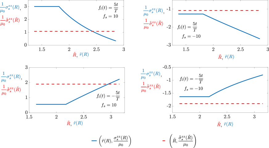
Figure 17: The $zz$-component of the Cauchy stress generated by a constant service load (Example 3.10). The solid-blue curves show the radial variation of the $zz$-component of the Cauchy stress in the $3$D-printed body. The dashed-red curves represent the same for a stress-free body of the same size and made of the same material as the $3$D-printed one.

The $3$D-printed body manufactured under the tensile load $f_{l}(t)=\frac{5t}{T}$ has tensile residual stress in its inner layers and compressive residual stress in the outer layers. As a result, when a tensile service load is applied, it always develops tensile stress in its inner layers while the stress in the outer layers can be compressive for very small service loads. For larger loads that causes tensile $\sigma_{s}^{zz}$ throughout the cross-section, $\sigma_{s}^{zz}$ is greater than $\accentset{\circ}{\sigma}_{s}^{zz}$ in the inner layers, while it is the opposite for the outer layers. If this body manufactured under the tensile load is subjected to compression, $\sigma_{s}^{zz}$ can still be tensile in the inner layers for small enough loads. It is possible to have slightly larger compressive service load so that the inner layers have compressive stress, but lesser than that of a stress-free body of same size subjected to the same load, while the outer layers follow the opposite trend. However, if the compressive service load is large enough, the stresses in the $3$D-printed body are more compressive than those of the stress-free body throughout the cross-section.

The residual stress in the $3$D-printed body manufactured under the compressive load $f_{l}(t)=-\frac{5t}{T}$ is compressive in its inner layers and tensile in the outer layers. If tensile service loads are large enough, $\sigma_{s}^{zz}$ in the $3$D-printed body is always tensile (with the inner layers being less stressed than the outer ones) but less stressed than the stress-free body of the same size subjected to the same service load. Similarly, if compressive service loads are large enough, $\sigma_{s}^{zz}$ in the $3$D-printed body is always compressive (with the inner layers being more stressed than the outer ones) but less stressed than the stress-free body of the same size subjected to the same service load.

4 Conclusions

In this paper we presented a geometric formulation of the nonlinear mechanics of accreting-ablating bodies. This theory models the large deformations of bodies that undergo simultaneous accretion and ablation on their boundaries. This is a generalization of the accretion theory that was formulated in [Sozio and Yavari, 2019]. In this formulation the natural (stress-free) configuration of the body is a time-dependent Riemannian manifold. Formulating the accretion-ablation boundary-value problem requires the construction of the material metric for the accreted portion of the body. For ablation we simply need a map to track the points on the boundary being ablated at any given time. However, we do not need to track the particles after they have left the body. The material metric is an unknown field a priori and is determined after solving the accretion-ablation initial-boundary-value problem. This theory is not restricted to isotropic materials; the initial body can be made of any anisotropic material. The accreting particles can be anisotropic as well. Also, the material points joining the body can be stressed at their time of attachment.

In the second part of the paper we considered an incompressible thick hollow cylinder undergoing accretion on its outer boundary and ablation on its inner boundary while it is being loaded axially. For the sake of simplicity, we assumed a homogeneous and isotropic material both in the initial body and accreting particles. Also, to simplify kinematics we assumed that the initial body is made of an incompressible solid. It is also assumed that the material that is added to the body during the accretion process is incompressible as well. We derived the governing equations for two cases: i) when $t<t_{\text{ablation}}$ a portion of the initial body is still present, and ii) the initial body has been completely ablated. Assuming constant accretion and ablation velocities we solved the problem for case i). We considered two different loading scenarios: displacement-control and force-control loadings. In the case of displacement-control loading we obtained a semi-analytical solution for the problem. Further, we calculated the residual stresses after the completion of the accretion-ablation processes and the removal of external forces. Given a time-dependent axial stretch during loading, we provided analytical expressions for both the residual stretch and axial residual stress.

A future extension of this work would be to study problems where the accretion and ablation velocities are dictated by mass transport and heat transfer. Studying large elastic deformations in accretion-ablation problems coupled with phase changes will be the subject of a future communication.

Appendix A The relation between $r(R,t)$ and $\lambda(t)$ for an accreting-ablating incompressible thick hollow cylinder under finite extension

The traction continuity equation (3.57) can be rearranged as follows:

$$\int_{S_{1}(t)}^{R_{2}}\left[\frac{1}{R}-\frac{R^{3}}{r^{4}(R,t)\lambda^{4}(t)}\right]\text{d}R+\int_{R_{2}}^{S_{2}(t)}\frac{\accentset{+}{\lambda}^{2}(R)}{\accentset{+}{r}(R)}\left[1-\frac{\accentset{+}{r}^{4}(R)\accentset{+}{\lambda}^{4}(R)}{r^{4}(R,t)\lambda^{4}(t)}\right]\text{d}R=0\,.$$ (A.1)

For the sake of convenience, let us denote

$$A(t):= \int_{S_{1}(t)}^{R_{2}}\left[\frac{1}{R}-\frac{R^{3}}{r^{4}(R,t)\lambda^{4}(t)}\right]\text{d}R\,,\qquad B(t):=\int_{R_{2}}^{S_{2}(t)}\frac{\accentset{+}{\lambda}^{2}(R)}{\accentset{+}{r}(R)}\left[1-\frac{\accentset{+}{r}^{4}(R)\accentset{+}{\lambda}^{4}(R)}{r^{4}(R,t)\lambda^{4}(t)}\right]\text{d}R=0\,.$$ (A.2)

Observe that (3.11) and (3.21) can be combined to write

$$r^{2}(R,t)\lambda^{2}(t)=\begin{dcases}s_{1}^{2}(t)\lambda^{2}(t)-S_{1}^{2}(t)+R^{2}\,,&R\leq R_{2}\,,\\ s_{1}^{2}(t)\lambda^{2}(t)-S_{1}^{2}(t)+R_{2}^{2}+2\int_{R_{2}}^{R}\accentset{+}{\lambda}^{2}(\zeta)\,\accentset{+}{r}(\zeta)\,\text{d}\zeta\,,&R\geq R_{2}\,.\end{dcases}$$ (A.3)

Let us define the following two functions

$$\chi(t):=s_{1}^{2}(t)\lambda^{2}(t)-S_{1}^{2}(t)\,,\qquad\psi(R):=\begin{dcases}R^{2}\,,&R\leq R_{2}\,,\\ R_{2}^{2}+2\int_{R_{2}}^{R}\accentset{+}{\lambda}^{2}(\zeta)\,\accentset{+}{r}(\zeta)\,\text{d}\zeta\,,&R\geq R_{2}\,,\end{dcases}$$ (A.4)

so that $r^{2}(R,t)\lambda^{2}(t)=\chi(t)+\psi(R)$. Further,

$$\psi^{\prime}(R)=\begin{dcases}2R\,,&R\leq R_{2}\,,\\ 2\accentset{+}{\lambda}^{2}(R)\,\accentset{+}{r}(R)\,,&R\geq R_{2}\,.\end{dcases}$$ (A.5)

Now, one can write

$$\dot{A}(t) =\int_{S_{1}(t)}^{R_{2}}\frac{\partial}{\partial t}\left[\frac{1}{R}-\frac{R^{3}}{r^{4}(R,t)\lambda^{4}(t)}\right]\text{d}R-\left[\frac{1}{S_{1}(t)}-\frac{S_{1}^{3}(t)}{r^{4}(S_{1}(t),t)\lambda^{4}(t)}\right]\dot{S_{1}}(t)$$ (A.6)

$$=-\int_{S_{1}(t)}^{R_{2}}\frac{\partial}{\partial t}\left[\frac{R^{3}}{[\chi(t)+\psi(R)]^{2}}\right]\text{d}R-\accentset{-}{\upsilon}\left[\frac{1}{S_{1}(t)}-\frac{S_{1}^{3}(t)}{s_{1}^{4}(t)\lambda^{4}(t)}\right]$$

$$=\int_{S_{1}(t)}^{R_{2}}\frac{2\dot{\chi}(t)R^{3}}{[\chi(t)+\psi(R)]^{3}}\text{d}R-\accentset{-}{\upsilon}\left[\frac{1}{S_{1}(t)}-\frac{S_{1}^{3}(t)}{s_{1}^{4}(t)\lambda^{4}(t)}\right]$$

$$=\frac{\dot{\chi}(t)}{4}\int_{S_{1}(t)}^{R_{2}}\frac{[\psi^{\prime}(R)]^{3}\text{d}R}{[\chi(t)+\psi(R)]^{3}}-\accentset{-}{\upsilon}\left[\frac{1}{S_{1}(t)}-\frac{S_{1}^{3}(t)}{s_{1}^{4}(t)\lambda^{4}(t)}\right]\,,$$

and

$$\dot{B}(t) =-\int_{R_{2}}^{S_{2}(t)}\frac{\partial}{\partial t}\left[\frac{\accentset{+}{r}^{3}(R)\accentset{+}{\lambda}^{6}(R)}{r^{4}(R,t)\lambda^{4}(t)}\right]\text{d}R+\frac{\accentset{+}{\lambda}^{2}(S_{2}(t))}{\accentset{+}{r}(S_{2}(t))}\left[1-\frac{\accentset{+}{r}^{4}(S_{2}(t))\accentset{+}{\lambda}^{4}(S_{2}(t))}{r^{4}(S_{2}(t),t)\lambda^{4}(t)}\right]\dot{S_{2}}(t)$$ (A.7)

$$=-\int_{R_{2}}^{S_{2}(t)}\frac{\partial}{\partial t}\left[\frac{\accentset{+}{r}^{3}(R)\accentset{+}{\lambda}^{6}(R)}{[\chi(t)+\psi(R)]^{2}}\right]\text{d}R$$

$$=\int_{R_{2}}^{S_{2}(t)}\frac{2\dot{\chi}(t)\,\accentset{+}{r}^{3}(R)\accentset{+}{\lambda}^{6}(R)}{[\chi(t)+\psi(R)]^{3}}\text{d}R$$

$$=\frac{\dot{\chi}(t)}{4}\int_{R_{2}}^{S_{2}(t)}\frac{[\psi^{\prime}(R)]^{3}\text{d}R}{[\chi(t)+\psi(R)]^{3}}\,.$$

Differentiating (A.1) with respect to time and using (A.6) and (A.7) one obtains

$$\frac{\dot{\chi}(t)}{4}\int_{S_{1}(t)}^{S_{2}(t)}\frac{[\psi^{\prime}(R)]^{3}\text{d}R}{[\chi(t)+\psi(R)]^{3}}=\accentset{-}{\upsilon}\left[\frac{1}{S_{1}(t)}-\frac{S_{1}^{3}(t)}{s_{1}^{4}(t)\lambda^{4}(t)}\right]\,.$$ (A.8)

Note that

$$\frac{1}{S_{1}(t)}-\frac{S_{1}^{3}(t)}{s_{1}^{4}(t)\lambda^{4}(t)}=\frac{\chi(t)\,\left[\,\chi(t)+2S_{1}^{2}(t)\,\right]\,}{S_{1}(t)\,\left[\,\chi(t)+S_{1}^{2}(t)\,\right]^{2}}\,,$$ (A.9)

and hence

$$\frac{\dot{\chi}(t)}{4}\int_{S_{1}(t)}^{S_{2}(t)}\frac{[\psi^{\prime}(R)]^{3}\text{d}R}{[\chi(t)+\psi(R)]^{3}}=\frac{\accentset{-}{\upsilon}\,\chi(t)\,\left[\,\chi(t)+2S_{1}^{2}(t)\,\right]\,}{S_{1}(t)\,\left[\,\chi(t)+S_{1}^{2}(t)\,\right]^{2}}\,.$$ (A.10)

Let us define

$$\gamma(t):=-\int_{0}^{t}\frac{4\accentset{-}{\upsilon}\,\left[\,\chi(\tau)+2S_{1}^{2}(\tau)\,\right]\text{d}\tau}{S_{1}(\tau)\,\left[\,\chi(\tau)+S_{1}^{2}(\tau)\,\right]^{2}\,\int_{S_{1}(\tau)}^{S_{2}(\tau)}\frac{[\psi^{\prime}(R)]^{3}}{[\chi(\tau)+\psi(R)]^{3}}\text{d}R}\,.$$ (A.11)

Thus, we have

$$\dot{\chi}(t)+\dot{\gamma}(t)\chi(t)=0\,,\quad\text{or}\qquad\frac{\text{d}}{\text{d}t}\left[e^{\gamma(t)}\chi(t)\right]=0\,.$$ (A.12)

Integrating this ODE one obtains

$$e^{\gamma(t)}\chi(t)=e^{\gamma(0)}\chi(0)\,.$$ (A.13)

Now since $\gamma(0)=0$, and $\chi(0)=0$ (as $s_{1}(0)=S_{1}(0)=R_{1}$ and $\lambda(0)=1$), we conclude that $\chi(t)=0$, i.e. $s_{1}^{2}(t)\lambda^{2}(t)=S_{1}^{2}(t)$ for all $t<t_{\text{ablation}}$. Thus,

$$r^{2}(R,t)\lambda^{2}(t)=\begin{dcases}R^{2}\,,&R\leq R_{2}\,,\\ R_{2}^{2}+2\int_{R_{2}}^{R}\accentset{+}{\lambda}^{2}(\zeta)\,\accentset{+}{r}(\zeta)\,\text{d}\zeta\,,&R\geq R_{2}\,,\end{dcases}$$ (A.14)

is independent of time. Further, substituting $t=\accentset{+}{\tau}(R)$ one obtains

$$\accentset{+}{r}^{2}(R)\accentset{+}{\lambda}^{2}(R)=R_{2}^{2}+2\int_{R_{2}}^{R}\accentset{+}{\lambda}^{2}(\zeta)\,\accentset{+}{r}(\zeta)\,\text{d}\zeta\,,$$ (A.15)

which when differentiated with respect to $R$ gives

$$\frac{\text{d}}{\text{d}R}\left[\accentset{+}{r}(R)\accentset{+}{\lambda}(R)\right]=\accentset{+}{\lambda}(R)\,.$$ (A.16)

Integrating this along with $\accentset{+}{r}(R_{2})=R_{2}$, we finally obtain

$$\accentset{+}{r}(R)=\frac{R_{2}+\int_{R_{2}}^{R}\accentset{+}{\lambda}(\xi)\text{d}\xi}{\accentset{+}{\lambda}(R)}\,,$$ (A.17)

and hence

$$r(R,t)=\begin{cases}\displaystyle\frac{R}{\lambda(t)}\,,&S_{1}(t)\leq R\leq R_{2}\,,\\[10.0pt] \displaystyle\frac{\accentset{+}{\lambda}(R)\,\accentset{+}{r}(R)}{\lambda(t)}\,,&R_{2}\leq R\leq S_{2}(t)\,.\end{cases}$$ (A.18)

References

- Abi-Akl and Cohen [2020] R. Abi-Akl and T. Cohen. Surface growth on a deformable spherical substrate. Mechanics Research Communications, 103:103457, 2020.
- Abi-Akl et al. [2019] R. Abi-Akl, R. Abeyaratne, and T. Cohen. Kinetics of surface growth with coupled diffusion and the emergence of a universal growth path. Proceedings of the Royal Society A, 475(2221):20180465, 2019.
- Amar and Goriely [2005] M. B. Amar and A. Goriely. Growth and instability in elastic tissues. Journal of the Mechanics and Physics of Solids, 53(10):2284–2319, 2005.
- Arutyunyan et al. [1990] N. K. Arutyunyan, V. Naumov, and Y. N. Radaev. A mathematical model of a dynamically accreted deformable body. part 1: Kinematics and measure of deformation of the growing body. Izv. Akad. Nauk SSSR. Mekh. Tverd. Tela, (6):85–96, 1990.
- Bergel and Papadopoulos [2021] G. L. Bergel and P. Papadopoulos. A finite element method for modeling surface growth and resorption of deformable solids. Computational Mechanics, 68:759–774, 2021.
- Brown and Goodman [1963] C. Brown and L. Goodman. Gravitational stresses in accreted bodies. In Proceedings of the Royal Society of London A: Mathematical, Physical and Engineering Sciences, volume 276, pages 571–576. The Royal Society, 1963.
- Doyle and Ericksen [1956] T. C. Doyle and J. L. Ericksen. Nonlinear elasticity. Advances in Applied Mechanics, 4:53–115, 1956.
- Drozdov [1998a] A. D. Drozdov. Continuous accretion of a composite cylinder. Acta Mechanica, 128(1), 1998a.
- Drozdov [1998b] A. D. Drozdov. Viscoelastic Structures: Mechanics of Growth and Aging. Academic Press, 1998b.
- Eckart [1948] C. Eckart. The thermodynamics of irreversible processes. IV. The theory of elasticity and anelasticity. Physical Review, 73(4):373–382, 1948.
- Efrati et al. [2009] E. Efrati, E. Sharon, and R. Kupferman. Elastic theory of unconstrained non-Euclidean plates. Journal of the Mechanics and Physics of Solids, 57(4):762–775, 2009.
- Epstein and Maugin [2000] M. Epstein and G. A. Maugin. Thermomechanics of volumetric growth in uniform bodies. International Journal of Plasticity, 16(7-8):951–978, 2000.
- Ericksen [1954] J. L. Ericksen. Deformations possible in every isotropic, incompressible, perfectly elastic body. Zeitschrift für Angewandte Mathematik und Physik, 5(6):466–489, 1954.
- Golgoon and Yavari [2018] A. Golgoon and A. Yavari. Line and point defects in nonlinear anisotropic solids. Zeitschrift für angewandte Mathematik und Physik, 69(3):81, 2018.
- Goodbrake et al. [2021] C. Goodbrake, A. Goriely, and A. Yavari. The mathematical foundations of anelasticity: Existence of smooth global intermediate configurations. Proceedings of the Royal Society A, 477(2245):20200462, 2021.
- Goriely [2017] A. Goriely. The Mathematics and Mechanics of Biological Growth. Springer Verlag, New York, 2017.
- Goriely et al. [2010] A. Goriely, D. E. Moulton, and R. Vandiver. Elastic cavitation, tube hollowing, and differential growth in plants and biological tissues. Europhysics Letters, 91(1):18001, 2010.
- Hodge and Papadopoulos [2010] N. Hodge and P. Papadopoulos. A continuum theory of surface growth. Proceedings of the Royal Society of London A, 466(2123):3135–3152, 2010.
- Kadish et al. [2005] J. Kadish, J. Barber, and P. Washabaugh. Stresses in rotating spheres grown by accretion. International Journal of Solids and Structures, 42(20):5322–5334, 2005.
- Kondo [1949] K. Kondo. A proposal of a new theory concerning the yielding of materials based on Riemannian geometry. The Journal of the Japan Society of Aeronautical Engineering, 2(8):29–31, 1949.
- Kondo [1950] K. Kondo. On the dislocation, the group of holonomy and the theory of yielding. Journal of the Society of Applied Mechanics of Japan, 3(17):107–110, 1950.
- Lychev [2011] S. Lychev. Universal deformations of growing solids. Mechanics of Solids, 46(6):863–876, 2011.
- Lychev and Manzhirov [2013a] S. Lychev and A. Manzhirov. The mathematical theory of growing bodies. finite deformations. Journal of Applied Mathematics and Mechanics, 77(4):421–432, 2013a.
- Lychev and Manzhirov [2013b] S. Lychev and A. Manzhirov. Reference configurations of growing bodies. Mechanics of Solids, 48(5):553–560, 2013b.
- Lychev et al. [2021] S. Lychev, K. Koifman, and N. Djuzhev. Incompatible deformations in additively fabricated solids: Discrete and continuous approaches. Symmetry, 13(12):2331, 2021.
- Manzhirov [1995] A. Manzhirov. The general non-inertial initial-boundaryvalue problem for a viscoelastic ageing solid with piecewise-continuous accretion. Journal of Applied Mathematics and Mechanics, 59(5):805–816, 1995.
- Manzhirov [2014] A. V. Manzhirov. Mechanics of growing solids: New track in mechanical engineering. In ASME 2014 International Mechanical Engineering Congress and Exposition, pages V009T12A039–V009T12A039. American Society of Mechanical Engineers, 2014.
- Marsden and Hughes [1983] J. Marsden and T. Hughes. Mathematical Foundations of Elasticity. Dover, 1983.
- Metlov [1985] V. Metlov. On the accretion of inhomogeneous viscoelastic bodies under finite deformations. Journal of Applied Mathematics and Mechanics, 49(4):490–498, 1985.
- Moulton and Goriely [2011] D. E. Moulton and A. Goriely. Anticavitation and differential growth in elastic shells. Journal of Elasticity, 102(2):117–132, 2011.
- Naghibzadeh et al. [2022] S. K. Naghibzadeh, N. Walkington, and K. Dayal. Accretion and ablation in deformable solids with an eulerian description: examples using the method of characteristics. Mathematics and Mechanics of Solids, 27(6):989–1010, 2022.
- Naumov [1994] V. E. Naumov. Mechanics of growing deformable solids: a review. Journal of Engineering Mechanics, 120(2):207–220, 1994.
- Ogden [1984] R. W. Ogden. Non-Linear Elastic Deformations. Dover, 1984.
- Ong and O’Reilly [2004] J. J. Ong and O. M. O’Reilly. On the equations of motion for rigid bodies with surface growth. International Journal of Engineering Science, 42(19):2159–2174, 2004.
- Ozakin and Yavari [2010] A. Ozakin and A. Yavari. A geometric theory of thermal stresses. Journal of Mathematical Physics, 51:032902, 2010.
- Papadopoulos and Hodge [2010] P. Papadopoulos and N. Hodge. On surface growth of actin networks. International Journal of Engineering Science, 48(11):1498–1506, 2010.
- Pence and Tsai [2005] T. J. Pence and H. Tsai. Swelling-induced microchannel formation in nonlinear elasticity. IMA Journal of Applied Mathematics, 70(1):173–189, 2005.
- Pence and Tsai [2006] T. J. Pence and H. Tsai. Swelling-induced cavitation of elastic spheres. Mathematics and Mechanics of Solids, 11(5):527–551, 2006.
- Pence and Tsai [2007] T. J. Pence and H. Tsai. Bulk cavitation and the possibility of localized interface deformation due to surface layer swelling. Journal of Elasticity, 87(2-3):161–185, 2007.
- Poincaré [1905] H. Poincaré. Science and Hypothesis. Science Press, 1905.
- Sadik and Yavari [2017a] S. Sadik and A. Yavari. On the origins of the idea of the multiplicative decomposition of the deformation gradient. Mathematics and Mechanics of Solids, 22(4):771–772, 2017a.
- Sadik and Yavari [2017b] S. Sadik and A. Yavari. Geometric nonlinear thermoelasticity and the time evolution of thermal stresses. Mathematics and Mechanics of Solids, 22(7):1546–1587, 2017b.
- Sadik et al. [2016] S. Sadik, A. Angoshtari, A. Goriely, and A. Yavari. A geometric theory of nonlinear morphoelastic shells. Journal of Nonlinear Science, 26(4):929–978, 2016.
- Simo and Marsden [1984] J. Simo and J. Marsden. Stress tensors, Riemannian metrics and the alternative descriptions in elasticity. In Trends and Applications of Pure Mathematics to Mechanics, pages 369–383. Springer, 1984.
- Skalak et al. [1982] R. Skalak, G. Dasgupta, M. Moss, E. Otten, P. Dullemeijer, and H. Vilmann. Analytical description of growth. Journal of Theoretical Biology, 94(3):555–577, 1982.
- Skalak et al. [1997] R. Skalak, D. Farrow, and A. Hoger. Kinematics of surface growth. Journal of Mathematical Biology, 35(8):869–907, 1997.
- Southwell [1941] R. Southwell. Introduction to the Theory of Elasticity for Engineers and Physicists. Oxford University Press, 1941.
- Sozio and Yavari [2017] F. Sozio and A. Yavari. Nonlinear mechanics of surface growth for cylindrical and spherical elastic bodies. Journal of the Mechanics and Physics of Solids, 98:12–48, 2017.
- Sozio and Yavari [2019] F. Sozio and A. Yavari. Nonlinear mechanics of accretion. Journal of Nonlinear Science, 29(4):1813–1863, 2019.
- Sozio and Yavari [2020] F. Sozio and A. Yavari. Riemannian and Euclidean material structures in anelasticity. Mathematics and Mechanics of Solids, 25(6):1267–1293, 2020.
- Sozio et al. [2020] F. Sozio, M. Faghih Shojaei, S. Sadik, and A. Yavari. Nonlinear mechanics of thermoelastic accretion. Zeitschrift für angewandte Mathematik und Physik, 71:1–24, 2020.
- Stojanovic et al. [1964] R. Stojanovic, S. Djuric, and L. Vujosevic. On finite thermal deformations. Archiwum Mechaniki Stosowanej, 16:103–108, 1964.
- Tomassetti et al. [2016] G. Tomassetti, T. Cohen, and R. Abeyaratne. Steady accretion of an elastic body on a hard spherical surface and the notion of a four-dimensional reference space. Journal of the Mechanics and Physics of Solids, 96:333–352, 2016.
- Truskinovsky and Zurlo [2019] L. Truskinovsky and G. Zurlo. Nonlinear elasticity of incompatible surface growth. Physical Review E, 99(5):053001, 2019.
- Yavari [2010] A. Yavari. A geometric theory of growth mechanics. Journal of Nonlinear Science, 20(6):781–830, 2010.
- Yavari and Goriely [2012a] A. Yavari and A. Goriely. Riemann-Cartan geometry of nonlinear dislocation mechanics. Archive for Rational Mechanics and Analysis, 205(1):59–118, 2012a.
- Yavari and Goriely [2012b] A. Yavari and A. Goriely. Weyl geometry and the nonlinear mechanics of distributed point defects. Proceedings of the Royal Society A, 468(2148):3902–3922, 2012b.
- Yavari and Goriely [2012c] A. Yavari and A. Goriely. Riemann–Cartan geometry of nonlinear disclination mechanics. Mathematics and Mechanics of Solids, 18(1):91–102, 2012c.
- Yavari and Goriely [2014] A. Yavari and A. Goriely. The geometry of discombinations and its applications to semi-inverse problems in anelasticity. Proceedings of the Royal Society A, 470(2169):20140403, 2014.
- Yavari and Pradhan [2022] A. Yavari and S. P. Pradhan. Accretion mechanics of nonlinear elastic circular cylindrical bars under finite torsion. Journal of Elasticity, pages 1–32, 2022.
- Yavari and Sozio [2023] A. Yavari and F. Sozio. On the direct and reverse multiplicative decompositions of deformation gradient in nonlinear anisotropic anelasticity. Journal of the Mechanics and Physics of Solids, 170:105101, 2023.
- Yavari et al. [2023] A. Yavari, Y. Safa, and A. Soleiman Fallah. Finite extension of accreting nonlinear elastic solid circular cylinders. Continuum Mechanics and Thermodynamics, pages 1–17, 2023.
- Zurlo and Truskinovsky [2017] G. Zurlo and L. Truskinovsky. Printing non-Euclidean solids. Physical Review Letters, 119(4):048001, 2017.
- Zurlo and Truskinovsky [2018] G. Zurlo and L. Truskinovsky. Inelastic surface growth. Mechanics Research Communications, 93:174–179, 2018.