Astrophysical calibration of the oscillator strengths of YJ-band absorption lines in classical Cepheids

Abstract

Newly-developed spectrographs with increased resolving powers, particularly those covering the near-IR range, allow the characterization of more and more absorption lines in stellar spectra. This includes the identification and confirmation of absorption lines and the calibration of oscillator strengths. In this study, we provide empirical values of ${\log gf}$ based on abundances of classical Cepheids obtained with optical spectra in Luck (2018), in order to establish the consistency between optical and infrared abundance results. Using time-series spectra of classical Cepheids obtained with WINERED spectrograph (0.97–1.35 $\mu$m, R $\sim$ 28000), we demonstrate that we can determine the stellar parameters of the observed Cepheids, including effective temperature (${T_{\mathrm{eff}}}$), surface gravity (${\log g}$), microturbulence ($\xi$), and metallicity (${\rm{[{M}/H]}}$). With the newly calibrated relations of line-depth ratios (LDRs), we can achieve accuracy and precision comparable to optical studies (Luck, 2018), with uncertainties of $\sim$ 90 K and 0.108 dex for ${T_{\mathrm{eff}}}$, and ${\log g}$, respectively. Finally, we created a new atlas of absorption lines, featuring precise abundance measurements of various elements found in the atmosphere of Cepheids (including neutron-capture elements), with ${\log gf}$ values that have been astrophysically calibrated.

1 Introduction

Infrared spectroscopic observations provide valuable means for studying astronomical targets that are heavily obscured by interstellar extinction, which is a significant advantage over optical observations. The availability of mid-to-high resolution infrared spectra has led to the detection of both strong and weak absorption lines, The NIR regime, in particular, the YJ bands, is a relatively understudied region that has the potential to yield significant new insights into the chemical evolution of the Galaxy.

Despite the importance of basic spectral information, such as line positions and strengths in understanding the overall spectral scenario, the atomic information relevant to each spectral feature has not been widely covered in the literature (Ryde et al., 2019). The calibration of these parameters is crucial for further procedures, such as estimating abundances. The oscillator strength (${\log gf}$) is a dimensionless quantity that measures the strength of a transition (absorption and emission). In the NIR regime, accurately estimated ${\log gf}$ values are often lacking (see, e.g., Andreasen et al., 2016), and proper line identification is also frequently absent.

It is important to note that the definitive atomic parameters that are currently missing in the infrared bands must ultimately be obtained through laboratory astrophysics. However, in order to ensure consistency between optical and infrared chemical abundance results, we aim to obtain the empirical (or astrophysical) ${\log gf}$ values based on the optical abundance results for Cepheids presented in Luck (2018). Such empirical calibrations also help to reduce the internal errors caused by the choice of the atmosphere model and, ultimately, improve our abundance measurements. The sample of Luck (2018) constitutes the largest collection of Cepheids that have been homogeneously analyzed for different elements in the optical range, making it an ideal data set for this purpose.

Cepheid variables are not only valuable for distance estimates, but their spectra also exhibit a considerable number of absorption lines, making them useful tracers of chemical abundances in their host galaxies, particularly in the case of the Galaxy. In particular, Cepheids have been proven to be useful for studying the metallicity gradient of the Galactic disk e.g., (Genovali et al., 2014; Luck, 2018). A key parameter in the spectroscopic analysis is the effective temperature, ${T_{\mathrm{eff}}}$. Once this intrinsic parameter is derived, the subsequent (but not less important) parameters, i.e., surface gravity (${\log g}$), microturbulent velocity ($\xi$), and metallicity (${\rm{[Fe/H]}}$) may be estimated with spectra. Besides the identification and calibration of absorption lines in Cepheids, we aim to exploit the capabilities of the unique high-resolution spectra with WINERED (Ikeda et al., 2022), by employing the empirical LDR method (Gray & Johanson, 1991). We follow the prescription made in the NIR by Matsunaga et al. (2021) but extend it for the first time in the ${T_{\mathrm{eff}}}$ and ${\log g}$ parameter space to cover the range of classical Cepheids.

This paper is organized as follows. In Section 2, we provide detailed information about the analyzed targets and the WINERED spectrograph, as well as the procedure employed to prepare the spectra for measurements. In Section 3, we discuss the capabilities of our data to provide precise and accurate stellar parameters (${T_{\mathrm{eff}}}$ and ${\log g}$, primarily) based on our extension of the LDR method. Section 4 presents our method to identify and confirm the lines we will use for abundance determination, as well as the derivation of microturbulence ($\xi$) and the calibration of the oscillator strengths (${\log gf}$). Based on the results in Section 4, we measured the abundances of Cepheids as we present in Section 5. We later discuss the scope and limitations of our results in Section 6.

2 Data

2.1 Observations and targets

We analyze multi-epoch spectra of eleven Cepheids in the solar neighborhood obtained with the WINERED spectrograph in its WIDE mode, which has a resolving power of R $\sim$ 28000. The observations were conducted from 2013 to 2016 at the 1.3 m Araki Telescope located at the Koyama Observatory of Kyoto Sangyo University in Japan. As given in Tables LABEL:tab:obs_log_calibrators and LABEL:tab:obs_log_val, our sample is divided into two groups, calibrators, and validators. The former consists of eight widely studied Cepheids for which there is a wealth of data sets available (photometric and spectroscopic). The latter consists of three Cepheids whose information in the literature is incomplete or scarce. For each target, we obtained multi-epoch spectra, with better phase coverage for the calibrators.

2.2 Pipeline reduction

During the observations, the nodding technique was employed to subtract the background radiation from the sky and the ambient facility. Two types of nodding patterns were used, “ABBA” and “OSO” (object-sky-object). We decided the nodding pattern for each observation to avoid latent signals after exposure of bright targets. Calibration data include flat fielding images and ThAr lamp spectra for wavelength calibration. The raw data were reduced by the WARP pipeline, created and developed by Hamano, S. . Every science target has more than a single exposure, and for different echelle orders, a combined 1D, air wavelength calibrated spectrum was obtained. The pipeline also outputs information about the signal-to-noise ratio (S/N) for each target at three different regions of each echelle order. A WINERED spectrum in the WIDE mode is divided into 20 echelle orders, of which we use the 11 orders covering 9760–10890 Å and 11800–13190 Å which are not heavily affected by telluric contamination.

Table 1: Observation Log (Calibrators)

Target	RA	DEC	Date and Time (UT)	JD	Phase	Exposures	Nodding
$\delta$ Cep	22:29:10.27	$+$58:24:54.7	2013-12-02 11:12	2456628.967	0.119	$188^{s}\times 3$	ABB
			2013-12-05 10:24	2456631.934	0.672	$188^{s}\times 2$	AB
			2013-12-25 10:07	2456651.922	0.396	$138^{s}\times 4$	OSO
			2015-08-06 13:09	2457241.048	0.178	$20^{s}\times 2$	OSO
			2015-08-08 13:49	2457243.076	0.556	$20^{s}\times 4$	ABBA
			2015-08-15 18:34	2457250.274	0.897	$30^{s}\times 2$	AB
			2015-10-23 12:51	2457319.036	0.711	$30^{s}\times 4$	OSO
$\eta$ Aql	19:52:28.37	$+$01:00:20.4	2014-09-16 13:00	2456917.042	0.743	$188^{s}\times 2$	AB
			2014-09-17 10:23	2456917.933	0.867	$18^{s}\times 4$	ABBA
			2015-08-06 12:33	2457241.023	0.887	$30^{s}\times 4$	ABBA
			2015-08-08 13:59	2457243.083	0.174	$30^{s}\times 4$	ABBA
			2016-03-21 19:58	2457469.332	0.700	$100^{s}\times 2$	OSO
			2016-03-26 19:46	2457474.324	0.395	$30^{s}\times 6$	OSO
			2016-05-14 18:36	2457523.275	0.216	$50^{s}\times 2$	OSO
FF Aql	18:58:14.75	$+$17:21:39.3	2015-08-06 14:48	2457241.117	0.594	$120^{s}\times 4$	OSO
			2015-08-07 15:23	2457242.141	0.823	$60^{s}\times 2$	OSO
			2016-03-17 19:13	2457465.301	0.737	$150^{s}\times 4$	OSO
			2016-03-21 18:41	2457469.279	0.627	$300^{s}\times 2$	OSO
			2016-04-19 17:49	2457498.243	0.105	$300^{s}\times 2$	AB
RT Aur	06:28:34.09	$+$30:29:34.9	2014-01-23 16:20	2456681.181	0.920	$228^{s}\times 4$	ABBA
			2015-10-28 18:53	2457324.287	0.422	$150^{s}\times 4$	ABBA
			2016-02-16 14:41	2457435.112	0.149	$300^{s}\times 2$	OSO
			2016-02-28 12:20	2457447.014	0.341	$300^{s}\times 2$	OSO
			2016-03-07 12:47	2457455.033	0.492	$150^{s}\times 2$	OSO
			2016-03-15 11:12	2457462.967	0.620	$300^{s}\times 4$	OSO
			2016-03-17 11:03	2457464.961	0.155	$200^{s}\times 4$	ABBA
			2016-03-21 13:13	2457469.051	0.252	$200^{s}\times 4$	OSO
			2016-03-23 12:05	2457471.004	0.776	$300^{s}\times 2$	AB
SU Cas	02:51:58.75	$+$68:53:18.6	2013-12-25 10:07	2456651.922	0.054	$588^{s}\times 4$	ABBA
			2015-08-15 18:50	2457250.285	0.014	$120^{s}\times 2$	AB
			2016-03-12 09:36	2457459.900	0.546	$300^{s}\times 2$	OSO
			2016-03-15 10:40	2457462.945	0.108	$300^{s}\times 2$	OSO
			2016-03-17 11:24	2457464.975	0.150	$300^{s}\times 4$	ABBA
SZ Tau	04:37:14.78	$+$18:32:34.9	2014-01-24 13:00	2456682.042	0.870	$288^{s}\times 4$	ABBA
			2016-02-18 12:12	2457437.009	0.639	$300^{s}\times 4$	ABBA
			2016-03-17 09:57	2457464.915	0.502	$300^{s}\times 2$	AB
			2016-03-21 09:59	2457468.916	0.772	$300^{s}\times 2$	OSO
			2016-03-25 11:00	2457472.959	0.056	$300^{s}\times 4$	ABBA
X Cyg	20:43:24.19	$+$35:35:16.1	2014-08-30 13:16	2456900.053	0.606	$188^{s}\times 4$	ABBA
			2014-09-15 13:03	2456916.044	0.582	$108^{s}\times 4$	ABBA
			2014-09-18 11:12	2456918.967	0.760	$108^{s}\times 2$	AB
			2014-10-15 11:13	2456945.968	0.408	$138^{s}\times 2$	AB
			2015-07-25 13:35	2457229.066	0.685	$300^{s}\times 4$	ABBA
			2015-10-26 10:49	2457321.951	0.353	$300^{s}\times 2$	OSO
			2016-03-17 19:58	2457465.332	0.103	$200^{s}\times 4$	OSO
			2016-05-04 19:06	2457513.296	0.030	$300^{s}\times 4$	ABBA
			2016-05-18 17:16	2457527.220	0.880	$300^{s}\times 5$	OSO
$\zeta$ Gem	07:04:06.5	$+$20:34:13.1	2013-02-22 11:38	2456345.985	0.534	$188^{s}\times 7$	OSO
			2013-02-23 14:35	2456347.108	0.645	$108^{s}\times 8$	OSO
			2013-02-27 12:01	2456351.001	0.028	$108^{s}\times 9$	OSO
			2013-03-03 14:38	2456355.110	0.433	$88^{s}\times 9$	OSO
			2013-11-29 15:08	2456626.131	0.133	$108^{s}\times 4$	ABBA
			2016-02-17 13:35	2457436.066	0.923	$100^{s}\times 4$	OSO
			2016-03-07 12:37	2457455.026	0.791	$60^{s}\times 2$	OSO
			2016-03-23 11:13	2457470.968	0.362	$180^{s}\times 4$	OSO
			2016-05-01 10:16	2457509.928	0.200	$30^{s}\times 4$	OSO
			2017-12-05 08:12	2458092.842	0.626	$30^{s}\times 2$	OSO

Table 2: Observation Log (Validators)

Target	RA	DEC	Date and Time (UT)	JD	Phase	Exposures	Nodding
DL Cas	00:29:58.59	$+$60:12:43.1	2015-07-31 17:36	2457235.234	0.743	$300^{s}\times 4$	ABBA
			2015-08-07 14:49	2457242.118	0.604	$600^{s}\times 2$	OSO
			2015-10-23 13:07	2457319.047	0.219	$300^{s}\times 4$	OSO
S Sge	19:56:01.26	$+$16:38:05.2	2015-10-26 10:29	2457321.937	0.940	$300^{s}\times 2$	OSO
			2016-03-21 19:01	2457469.293	0.520	$300^{s}\times 2$	OSO
			2016-03-26 19:36	2457474.317	0.119	$300^{s}\times 2$	AB
T Vul	20:51:28.24	$+$28:15:01.8	2015-08-08 15:47	2457243.158	0.138	$200^{s}\times 4$	ABBA
			2016-05-14 18:48	2457523.284	0.293	$150^{s}\times 2$	OSO

2.3 Telluric correction and continuum normalization

The analysis of infrared spectra is subject to telluric contamination, caused by the Earth’s atmosphere. The telluric lines vary depending on factors such as the observatory location, weather conditions, and air mass. In order to accurately identify and study stellar features, it is necessary to remove telluric contamination from the observed spectra. In this study, the method developed in Sameshima et al. (2018) was employed to correct for the telluric contamination in the telluric standard stars observed in conjunction with the science targets. This correction was applied to every target and every order, with the exception of orders 53 and 54, corresponding to the spectral range covering $\lambda:[10280-10680]$ where the telluric absorption in our atmosphere can be neglected. The resulting spectra were then normalized by means of the IRAF continuum task to account for any offset from unity.

3 Stellar Parameters

3.1 Phased parameters from literature data

For the calibrators, we derived ${T_{\mathrm{eff}}}$, ${\log g}$, and $\xi$ at each phase from the interpolated Fourier curves based on the catalog of Luck (2018), which provides the measurement of these parameters with good phase sampling. We adopted the interpolated values for further analysis and calibrations. On the other hand, a different approach was applied to the validators by employing the Line-Depth Ratio (LDR) method.

3.2 Construction of LDR relations

The LDR method is widely used for determining the effective temperature (${T_{\mathrm{eff}}}$) in spectroscopic analysis. Previous studies were primarily conducted on optical spectra (Gray & Brown, 2001; Kovtyukh, 2000, 2007, and references therein), while more recent works have been involved with infrared spectra (Fukue et al., 2015; Taniguchi et al., 2018; Jian et al., 2019). However, all of these previous studies were limited to certain temperature ranges which do not include warmer Cepheids (${T_{\mathrm{eff}}}>6000$ K). Furthermore, LDRs used in the previous works tend to exhibit dependency not only on ${T_{\mathrm{eff}}}$ but also on ${\log g}$ and metallicity (Jian et al., 2019, 2020). In order to bypass such complexities, Taniguchi et al. (2021) proposed to use only Fe i lines to estimate ${T_{\mathrm{eff}}}$, followed by the work of Matsunaga et al. (2021), introducing the usage of neutral-ionized pairs to give the LDR relations with ${\log g}$, setting the guideline of this study.

In this work, the LDR method is employed following the prescription stated in Matsunaga et al. (2021) by using Fe i, Fe ii, Ca i, and Ca ii within 9760–10860 Å and 11800–13190 Å corresponding to the WINERED echelle orders in the $Y$ band (52nd–57th) and the $J$ band (43rd–47th). From Matsunaga et al. (2021), we adopted the list of 97 lines for the four species (76 Fe i, 5 Fe ii, 11 Ca i and 5 Ca ii), but we searched for new line pairs that show good LDR relations. According to our preliminary test on our sample of Cepheids, the LDR relations presented in Matsunaga et al. (2021) do not work well in hotter targets (${T_{\mathrm{eff}}}>6000$ K) as some lines are too shallow at high temperatures. It is worth mentioning that other elements were found in the spectra such as Si and Ti displaying both neutral and ionized lines but the number of ionized lines is very limited.

In order to measure the depth of each of the 97 lines from Matsunaga et al. (2021), a Gaussian fit was performed on the section of five pixels around the line center ($\lambda_{c}$). The wavelength of the line minimum ($\lambda_{0}$) was then determined, and assuming that the continuum normalization was properly done, the depth was calculated as the “distance” from the continuum level (the unity) to the flux at $\lambda_{0}$. We rejected measurements if the continuum level was not well normalized and the estimated depth was a negative number, or if the position of $\lambda_{0}$ was too far from $\lambda_{c}$. This procedure was carried out using the $ir\_ldr$ python package developed by Jian, M. . The error in each depth measurement is linked to the signal-to-noise ratio (S/N) for the target (obj) and the telluric standard (tell), and the two errors were added in quadrature:

$$e=\sqrt{e^{2}_{obj}+e^{2}_{tell}}=\sqrt{\Bigg{(}\frac{1}{(S/N)_{obj}}\Bigg{)}^{2}+\Bigg{(}\frac{1}{(S/N)_{tell}}\Bigg{)}^{2}}$$ (1)

This equation was used for all the WINERED echelle orders except for the orders 53 and 54, for which no telluric correction was performed, as they cover the wavelength ranges corresponding to an atmospheric window free of telluric absorption. For those two orders, the error is simply $e=e_{obj}$. We created a new list of line pairs that are effective in the Cepheids regime 5500 K $<$ ${T_{\mathrm{eff}}}$ $<$ 6500 K, following the algorithm of pair selection in Matsunaga et al. (2021, Section 3.3).

Table 3: LDR relations

ID	Line 1	Line 2	Form ID	Form (ext)	$\alpha$	$\beta$	$\gamma$	$\sigma_{y}$	$\sigma_{p}$
(1)	FeI 10155.162	FeI 10353.804	T4	21.655	$-5.781$	—	0.0506	109	39
(2)	FeI 10167.468	FeI 10347.965	T4	21.630	$-5.812$	—	0.0587	126	39
(3)	FeI 10195.105	FeI 10216.313	T3	2.4913	$-5.657\times 10^{-4}$	—	0.0659	117	46
(4)	FeI 10218.408	FeI 10227.994	T2	74.224	$-19.296$	—	0.2475	159	43
(5)	FeI 10340.885	FeI 10532.234	T2	18.883	$-4.816$	—	0.0407	105	50
(6)	FeI 10395.794	FeI 9861.7337	T2	18.502	$-4.697$	—	0.0401	106	45
(7)	FeI 10423.743	FeI 10863.518	T2	22.176	$-5.767$	—	0.0472	102	37
(8)	FeI 10577.139	FeI 10849.465	T2	27.377	$-7.163$	—	0.0729	126	34
(9)	FeI 10616.721	FeI 9868.1857	T2	21.268	$-5.594$	—	0.0583	130	32
(10)	FeI 10783.050	FeI 9889.0351	T2	17.597	$-4.530$	—	0.0465	128	44
(11)	FeI 10818.274	FeI 9811.5041	T4	16.784	$-4.478$	—	0.0391	108	42
(12)	FeI 12556.996	FeI 12648.741	T2	21.438	$-5.559$	—	0.0624	139	31
(13)	FeI 9868.1857	FeII 9997.5980	TG4	26.300	$-7.183$	$0.2368$	0.0506	0.21	74
(14)	FeI 10347.965	FeII 10173.515	TG3	1.9293	$-4.147\times 10^{-4}$	$0.2456$	0.0698	0.28	57
(15)	FeI 10353.804	FeII 10366.167	TG4	37.969	$-10.217$	$0.2699$	0.0750	0.28	60
(16)	FeI 10611.686	FeII 10501.500	TG3	2.0781	$-4.782\times 10^{-4}$	$0.2261$	0.0489	0.22	88
(17)	FeI 10818.274	FeII 10862.652	TG3	3.7638	$-7.925\times 10^{-4}$	$0.2587$	0.0639	0.25	61
(18)	CaI 10838.970	CaII 9854.7588	TG2	19.853	$-5.306$	$0.2080$	0.0666	0.32	66
(19)	CaI 10343.819	CaII 9890.6280	TG2	44.573	$-11.798$	$0.3498$	0.1147	0.33	75
(20)	CaI 10846.792	CaII 9931.3741	TG2	7.5153	$-2.013$	$0.0829$	0.0369	0.45	65
(21)	CaI 12105.841	CaII 11838.997	TG2	5.2987	$-1.427$	$0.0657$	0.0300	0.46	69
(22)	CaI 13033.554	CaII 11949.744	TG2	11.193	$-2.990$	$0.1109$	0.0328	0.30	71

To begin with the construction of our LDR relations, we use Fe i–Fe i pairs for estimating ${T_{\mathrm{eff}}}$, by pairing lines of low and high excitation potential (having a $\Delta\mathrm{EP}\geq 1$ eV) gives higher sensitivity to ${T_{\mathrm{eff}}}$ and their ratio can provide good diagnostics on temperature, reaching the utmost precision of $\sim$ 10 K (Gray & Johanson, 1991). Thus, the LDR of each pair is defined as $r=d_{\mathrm{low}}/d_{\mathrm{high}}$, i.e., the ratio of the depth of the line with a lower excitation potential ($d_{\mathrm{low}}$) to the depth of the line with a higher excitation potential ($d_{\mathrm{high}}$). We consider the four forms of the relation between $r$ and ${T_{\mathrm{eff}}}$ as described in Matsunaga et al. (2021, Section 3.4.1). We have 57 spectra of the calibrators in total, but the quality of the spectra shrank our sample to 51 (listed in table  LABEL:tab:obs_log), as well as the validation of measured depths may reduce the number of useful depths and according to the number of ratios. We rejected the line pairs for which only 30 or fewer validated measurements of $r$ were available and those for which the LDR relations had dispersion larger than 200 K. In addition, the range of ${T_{\mathrm{eff}}}$ covered by the points used for the fitting must be larger than 1000 K. This last condition is considered in order to make each LDR relation useful for a wide range of targets. For each line pair, one of the four forms (T1)–(T4) was selected to give the most negligible dispersion.

Surface gravity (${\log g}$) is also key in deriving subsequent stellar parameters, and analogously to ${T_{\mathrm{eff}}}$ there are multiple ways to estimate it. Its calculation is, however, not trivial. Some approaches rely on numerical models that are computationally expensive, and others depend on how stellar masses and radii can be estimated with photometry and interferometry. In order to estimate ${\log g}$, we consider pairs of neutral and ionized lines, i.e., Fe i–Fe ii and Ca i–Ca ii pairs taken from the line list of Matsunaga et al. (2021). Their LDRs are defined as

$r=d_{\mbox{{Fe\,{{i}}}}}/d_{\mbox{{Fe\,{{ii}}}}}$ or $r=d_{\mbox{{Ca\,{{i}}}}}/d_{\mbox{{Ca\,{{ii}}}}}$.

We selected the set of the LDR relations, among those which were not rejected, in order to include each line only in one line pair. We finally obtained 12 Fe i–Fe i, 5 Fe i–Fe ii, and 5 Ca i–Ca ii relations (Table 3).

3.3 Application of LDR relations

Using the relations we obtained in Section  3.2, we can determine ${T_{\mathrm{eff}}}$ and ${\log g}$ as follows:
(1) First, the LDR for each of the Fe i–Fe i pairs can be converted to an estimate of effective temperature, $T_{i}$. We also estimate its error, $e_{i}$, considering the error in the LDR and the scatter of the LDR relation ($\sigma_{p}$ in Table 3). Then, we calculate the weighted average and its standard error by

$$T_{\mathrm{LDR}} = \sum_{i=1}^{N_{\mathrm{pair}}}w_{i}T_{\mathrm{LDR},i}\Big{/}\sum_{i=1}^{N_{\mathrm{pair}}}w_{i}$$ (2)

$$e_{T} = \sqrt{\frac{\sum_{i=1}^{N_{\mathrm{pair}}}w_{i}(T_{\mathrm{LDR},i}-T_{\mathrm{LDR}})^{2}}{(N_{\mathrm{pair}}-1)\sum_{i=1}^{N_{\mathrm{pair}}}w_{i}}}$$ (3)

where $w_{i}$ is a weight given by $1/e_{i}^{2}$.
(2) We then estimate the LDR-based surface gravity by using the ${T_{\mathrm{LDR}}}$ obtained above. Based on each LDR relation of a Fe i–Fe ii pair or a Ca i–Ca ii pair, we obtain an estimate of surface gravity, ${\log g}_{i}$, and its error. Then, we calculate the weighted mean (${\log g_{\mathrm{LDR}}}$) and the error according to the formulae similar to Equations (2) and (3).

Figure 1 summarizes the results for ${T_{\mathrm{LDR}}}$ and ${\log g_{\mathrm{LDR}}}$ we obtained for the calibrators together with the results for the validators. The derived ${T_{\mathrm{eff}}}$ and ${\log g}$ for each phase are listed in the supplementary material. The deviations of ${T_{\mathrm{LDR}}}$ and ${\log g_{\mathrm{LDR}}}$ from those expected from the literature time-series data show the standard deviations $\sim 90$ K and $\sim 0.2$ dex. Larger errors are found at higher temperatures for ${T_{\mathrm{LDR}}}$ or at both higher and lower temperatures for ${\log g_{\mathrm{LDR}}}$. Absorption lines of neutral atoms tend to get weak at higher temperatures, while lines of ions tend to get weak at lower temperatures within the range of interest. This trend is observed in the number of the line pairs in the bottom panels and explains the larger deviations and errors seen in the middle panels. The standard deviation of ${T_{\mathrm{LDR}}}$, $\sim$ 90$\,K$, is larger than 42 K found by Matsunaga et al. (2021) for stars with $4800\leq{T_{\mathrm{eff}}}\leq 6200$ K and $1.35\leq{\log g}\leq 4.5$, while the standard deviation of ${\log g_{\mathrm{LDR}}}\sim 0.2$ dex, is similar to 0.17 dex obtained in the aforementioned work. The larger standard deviation of ${T_{\mathrm{LDR}}}$ can be ascribed to the fact that our sample includes significantly more stars with higher temperatures. The errors depend also on $S/N$. We will discuss this point in Section 6.

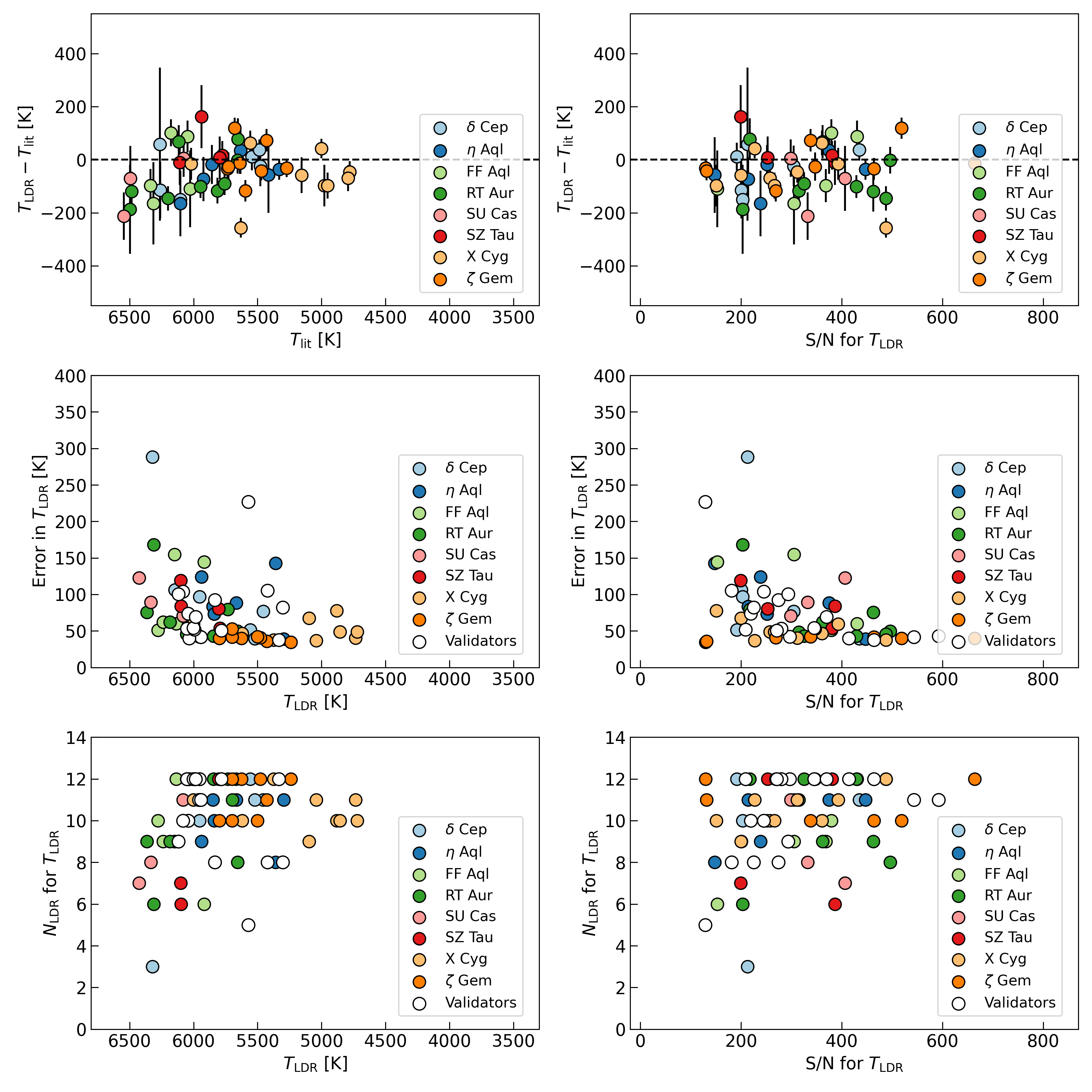
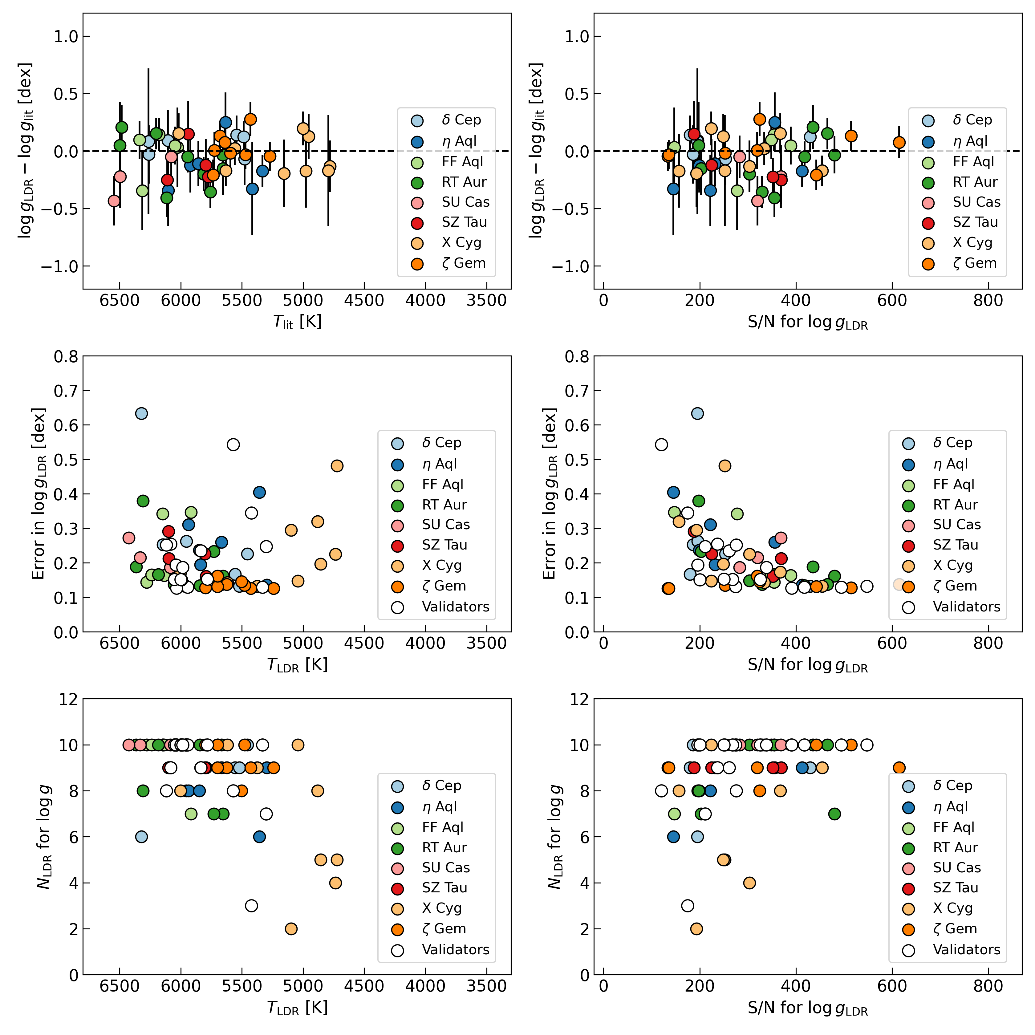
Figure 1: Performance of our LDR method for ${T_{\mathrm{eff}}}$ and ${\log g}$

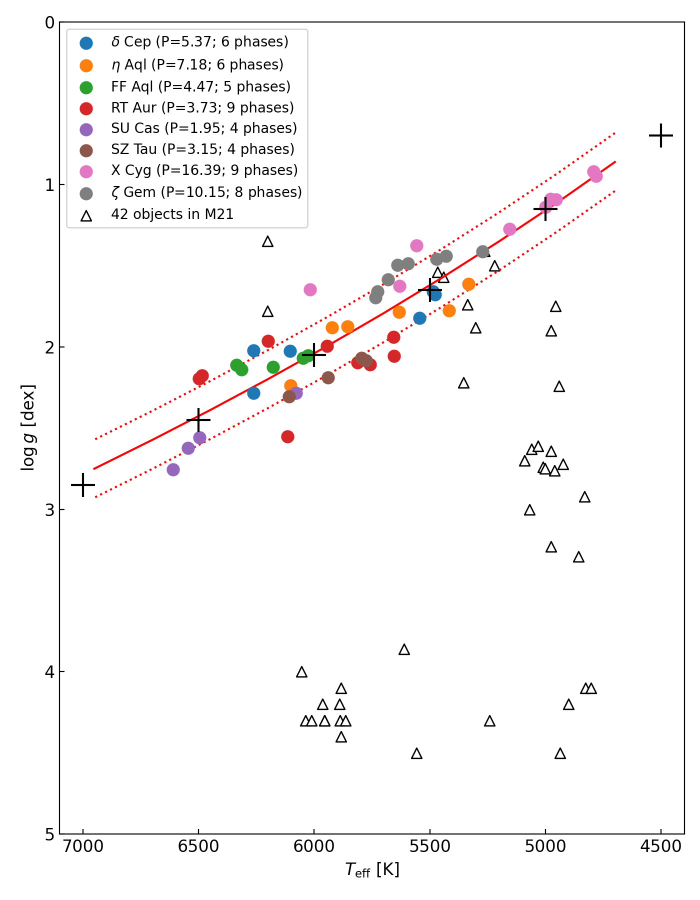
Figure 2: Distribution of the (${T_{\mathrm{eff}}},{\log g}$) of the Calibrator Cepheids given in the literature (Luck & Andrievsky, 2004; Luck et al., 2008; Andrievsky et al., 2005; Kovtyukh et al., 2005) plotted altogether with the sample of 42 FGK stars (M21) from Matsunaga et al. (2021)

3.4 Dependency of ${\log g}$ on ${T_{\mathrm{eff}}}$ and P

Looking at the (${T_{\mathrm{eff}}},{\log g}$) obtained with the literature curves, for the calibrators sample, it can be noted that the two parameters are tightly correlated (Figure 2). Such a correlation can be expected given the fact that the mean stellar parameters of Cepheids fall within the Cepheid instability strip, i.e., their mean ${T_{\mathrm{eff}}}$, ${\log g}$, and also the luminosity L should be (anti-) correlated. However, ${T_{\mathrm{eff}}}$ at individual phases are not necessarily within the instability strip. Moreover, the variations of ${T_{\mathrm{eff}}}$ and L do not follow the trend of the instability strip. A Cepheid becomes fainter when it gets cooler, while the instability strip makes fainter Cepheids warmer on average. Nevertheless, Figure 2 shows a tight correlation between ${T_{\mathrm{eff}}}$ and ${\log g}$ at individual phases of the calibrator Cepheids. Fitting the 51 points available for 8 calibrators in total, we obtained the relation,

$${\log g}=11.110\cdot\,\log({T_{\mathrm{eff}}}/5800)+1.877$$ (4)

with a scatter of 0.179 dex.

Furthermore, we found that including the $\log P$ term reduces the scatter. As illustrated in Figure 3, the residual around the ${T_{\mathrm{eff}}}$–${\log g}$ without the $\log P$ relation shows the dependency on the period. With the $\log P$ term included, we obtained the relation,

$${\log g}=6.483\cdot\log({T_{\mathrm{eff}}}/5800)-0.775\cdot\log P+2.475$$ (5)

with the scatter of 0.108 dex. This is smaller than the errors in the ${\log g_{\mathrm{LDR}}}$ presented above. It is hard to estimate ${\log g}$ with such high precision based solely on spectra (Mészáros et al., 2013). Although this relation is subject to systematic errors in Luck (2018), we can robustly obtain ${\log g}$ that would allow the abundance measurements to be consistent with the results in Luck (2018). The derived stellar parameters are found in detail in Appendix A.

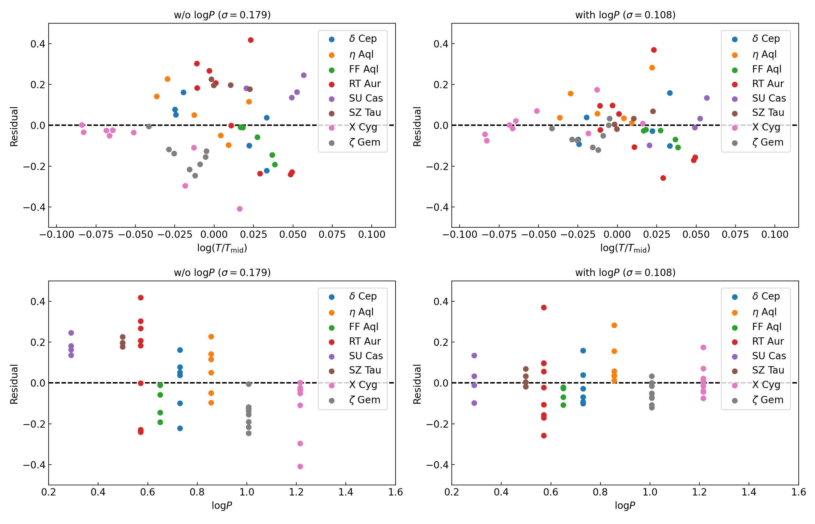
Figure 3: ${T_{\mathrm{eff}}}$–${\log P}$–${\log g}$ trend, displaying the dispersion when the pulsation period $P$ is included (right) or not (left) in the relation. $T_{\mathrm{mid}}=5800$.

Therefore, once ${T_{\mathrm{LDR}}}$ gets estimated, we can use the relation (5) to estimate the surface gravity of classical Cepheids. Let us denote thus-estimated surface gravity as ${\log g_{\mathrm{trend}}}$. For the precision of ${\log g_{\mathrm{trend}}}$, we need to take into account the temperature error. A moderately large error of 100 K in ${T_{\mathrm{LDR}}}$ would lead roughly to the error of 0.12 dex in ${\log g_{\mathrm{trend}}}$ combined with the scatter of the ${T_{\mathrm{eff}}}$–${\log g}$–$\log P$ relation. Using ${\log g_{\mathrm{trend}}}$ is, therefore, more accurate and robust than using ${\log g_{\mathrm{LDR}}}$.

4 Line selection and calibration

4.1 Line Selection

In this section, we discuss the line list to use for the abundance analysis. The first step is to select lines that are useful for measuring the abundances of different elements in the atmosphere of Cepheids. Concerning Fe i, we adopt the list of lines selected from VALD3 (Ryabchikova et al., 2015) and MB99 (Meléndez & Barbuy, 1999) that were compiled by Kondo et al. (2019). We also include other elements, among these lines we have Si i, S i, Ca i, Ca ii, Fe ii, Zn i, Y ii, and Dy ii from VALD and MB99 line lists. Most of the lines were confirmed and validated by examining the time-series high-resolution spectra we had available for this study. Figure 4 illustrates the absorption lines of different elements in our sample, the extended atlas of identified lines can be found in the supplementary online material.

Figure 4: Species found in order 53 (Y band) for three calibrators, SU Cas, $\delta$ Cep, and X Cyg. Lines in gray correspond to those found in Fukue et al. (2021), while those in red correspond to those newly found in this study.

For the species other than , we searched for candidate lines using synthetic spectra with MOOG (Sneden et al., 2012) considering a set of typical stellar parameters for Cepheids (${T_{\mathrm{eff}}}=5900$ K, ${\log g}=2.0$, ${\rm{[Fe/H]}}=0.0$). We employed the stellar atmosphere models from MARCS (Gustafsson et al., 2008) (${\rm{[{M}/H]}}\in[-2.5,0.5]$) spherical geometry for 5 $M_{\odot}$. The solar abundances in MARCS models are those of Grevesse et al. (2007), we converted them to the Asplund et al. (2009) scale. Potential candidates were then filtered according to the following criteria:

• They have to be deep enough ($d>0.03)$

• Blending ratio (the fraction of the EW of contaminating lines, $\beta_{1}$, defined in Kondo et al. (2019)) less than 0.3.

• Having a wide (${T_{\mathrm{eff}}}$, ${\log g}$) range, $\Delta{T_{\mathrm{eff}}}=1000K$, $\Delta{\log g}=1.0$.

The selection of lines resulted in 75 lines from VALD and 64 lines from MB99, and for the species other than Fe i. Including Fe i, the line list contains 105 lines from VALD and 90 lines from MB99.

We consider the line information obtained from VALD and MB99 separately. If the same line appears in both lists, we calibrate its $\log gf$ and measure the abundance using the line twice. In the analyses with each line list, we use each list for all metallic lines the atomic lines, including other species.

4.2 Line-by-line abundance

The abundance inferred from an individual line is estimated by iteratively searching for the set of free parameters, including the abundance of interest, line broadening, wavelength shift, and continuum normalization factor that results from the synthetic spectrum reproducing the observed spectrum with the minimal residual. We employ the OCTOMAN code (Taniguchi et al. in prep.), which performs such optimization based on the MPFIT algorithm by Takeda (1995). This algorithm has been utilized in various applications, including studies conducted with WINERED spectra (Kondo et al., 2019; Fukue et al., 2021).

The utilization of the OCTOMAN tool for estimating abundances may encounter difficulties in certain scenarios. For instance, when blended lines are present but not accurately represented in the synthetic spectra, the fitting process may be compromised, resulting in unreliable estimates of the parameters including the abundance. In such cases, it is appropriate to reject the measurements. For each absorption line, we measured the abundance as a function of microturbulence. We considered a grid with 24 different $\xi$ values ranging from 1.4 to 6.0 km s^-1 with the step of 0.2 km s^-1. Each run of OCTOMAN was performed for a fixed $\xi\in[1.4-6.0]$ for each spectrum.

Due to the effect of line saturation, the abundance obtained in each OCTOMAN run depends on $\xi$. As illustrated in the example in Figure 5, different lines show different trends of abundance against $\xi$. Deep lines show higher dependency on $\xi$ because they are more saturated, while weaker lines show little dependency. When many lines are strong and show the dependency on $\xi$, the averaged abundance itself depends on $\xi$, i.e., the estimates of abundance and $\xi$ show degeneracy. In contrast, if the majority of the lines are weak and depend little on $\xi$, the final estimate of abundance is more-or-less independent of the estimated $\xi$.

In some cases, the OCTOMAN failed to give reasonable abundances for a part of the $\xi$ grid points. The rejection criteria for the OCTOMAN outputs consider the parameters, niter, fwhmv, rv, and cnorm. The OCTOMAN measurements that passed the mentioned criteria are considered good when we have 19 or more grid points of $\xi$ for each line. Also, when we encounter $\xi-{\rm{[{X}/H]}}$ curves displaying a significant upturn by more than 0.05 dex, that means, if we find that the value of ${\rm{[{X}/H]}}$ at the largest grid point of $\xi$ is higher than the ${\rm{[{X}/H]}}$ at the smallest $\xi$ by 0.05 dex or more, that curve will be rejected. Thus, we accept curves having a sufficient number of good measurements showing a flat or decreasing trend over $\xi$. Otherwise, we reject the measurements of a given line entirely if we get less than 20 measurements over the $\xi$ grid.

The accepted curves for Fe i lines are used when we determine $\xi$ in Section  5.1. Also, for other species, examining such trends is useful to see how the microturbulence affects the measured abundance. Moreover, we use a plot like Figure 5 to identify the absorption lines whose measurements for a particular spectrum need to be rejected. We calculate the mean and standard deviation, $\sigma$, at each $\xi$ grid point. The solid black curve in Figure 5 indicates the curve of mean, while the dashed curves indicate the upper and lower limits (the mean $\pm 2\,\sigma$). Because of the different dependency on $\xi$, some curves of good measurements (especially the lines showing strong dependency on $\xi$) may well get outside the range between the upper and lower limits at some $\xi$. However, we reject the absorption lines whose curve in the $\xi$–[X/H] diagram is outside the limits at all the $\xi$ grid points. We make this rejection of the outlying curves once and re-calculate the mean and standard deviation at each $\xi$.

Figure 5: Fe i abundances as a function of microturbulence. The case of $\eta$ Aql.

4.3 Calibrating the oscillator strengths

We calibrate the ${\log gf}$ values of absorption lines present in Cepheids using our spectra of the calibrators. We assume that the stellar parameters including the microturbulence ($\xi$) are known for each phase of spectroscopic observation. For the calibrators, as mentioned above, we obtained the stellar parameters (${T_{\mathrm{eff}}},{\log g},\xi$) at each phase of our observations with the WINERED by interpolating the curve of each parameter given by Luck (2018). For each combination of absorption line and spectrum, we run the OCTOMAN to get the abundance. The deviation $\Delta{\log gf}$ of this abundance from the known abundance (Luck, 2018) includes, together with other errors, the offset in ${\log gf}$.

We find that the $\Delta{\log gf}$ values obtained for deep lines tend to show large systematic offsets. This trend is clearer in the elements with both weak lines and very strong lines like Si i, more than Fe i. Figures 8–8 show all the available $\Delta{\log gf}_{i}$ values for the case of neutral Si. The $\Delta{\log gf}_{i}$ values tend to be positive at depths larger than 0.2 - 0.25. This may be partly attributed to a systematic trend buried in the original ${\log gf}$ values in VALD and MB99. However, such a systematic trend of $\Delta{\log gf}$ exceeding 0.5 dex for all strong lines is unexpected. It is instead understood as the limitation of using fixed microturbulence. As we discuss in more detail in Section 6, the microturbulence is expected to be significantly larger in the upper layers of the stellar atmosphere. Trying to calibrate ${\log gf}$ with underestimated $\xi$ would lead to overestimates as we see here. We thus use the measurements for lines shallower than 0.2 in depth (the separation of the absorption core from the continuum level in each observed spectrum). In addition, among $\Delta{\log gf}$ of the not-too-strong lines, we reject outliers with the $2\,\sigma$ clipping according to the standard deviation.

Without including the measurements of lines whose depths were more than 0.2, we demand having more than 20 good measurements for each line in order to proceed with the calculations of new ${\log gf}$. The accepted measurements made a toll of 97 lines for VALD and 86 lines for MB99. Subsequently, OCTOMAN was run for each of the accepted lines in order to obtain the abundance of each of the elements, let us denote it as ${\rm{[{X}/H]}}$, as a function of $\xi$.

For the accepted $\xi-{\rm{[{X}/H]}}$ curves, we estimate the ${\rm{[{X}/H]}}$ at the $\xi$ given (expected) from the Luck (2018) dataset (Section 3), and thus, we can obtain the necessary shift to match the literature ${\rm{[{X}/H]}}_{lit}$ values. We denominate such an offset given by each spectrum ($\Delta{\log gf}_{i}$), and calculate the mean of it from all the spectra that give accepted measurements for the particular line. In order to calculate the mean we need 20 or more $\Delta{\log gf}_{i}$ values. The final error of the calibrated ${\log gf}$ of this offset is obtained by calculating the standard deviation of the $\Delta{\log gf}_{i}$. This calibration was effective enough for 42 VALD lines and 37 MB99 lines for Fe I, and for 48 VALD lines and 37 MB99 lines for the species different that Fe I. The results of this procedure are given in Table LABEL:tab:calib_Fe1_loggf and Table LABEL:tab:calib_species_loggf given in Appendix B.

Figure 6: The offsets between the original and new ${\log gf}$ values in our calibration for the lines taken from VALD (upper) and MB99 (middle).

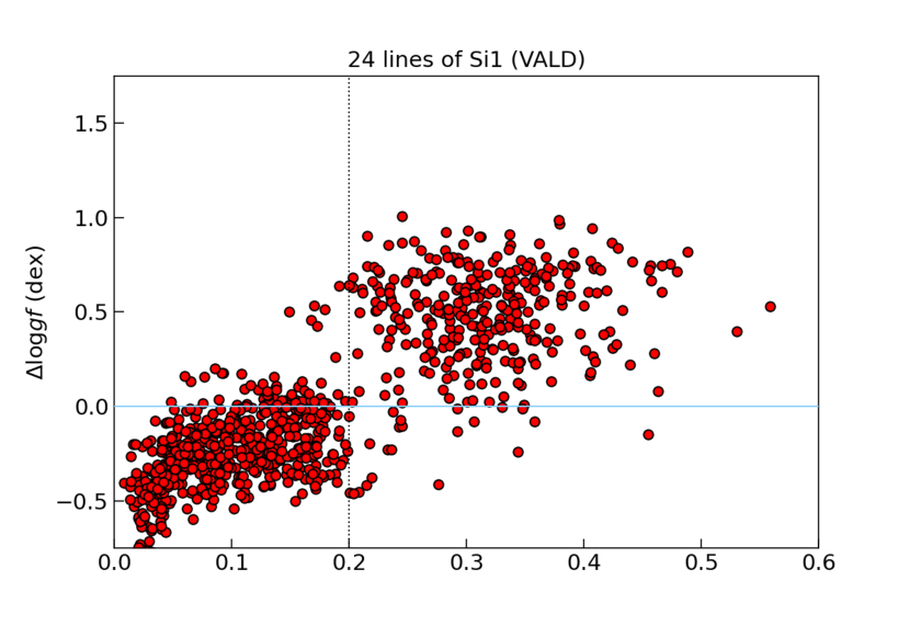
Figure 7: $\Delta{\log gf}_{i}$ for Si i lines from VALD.

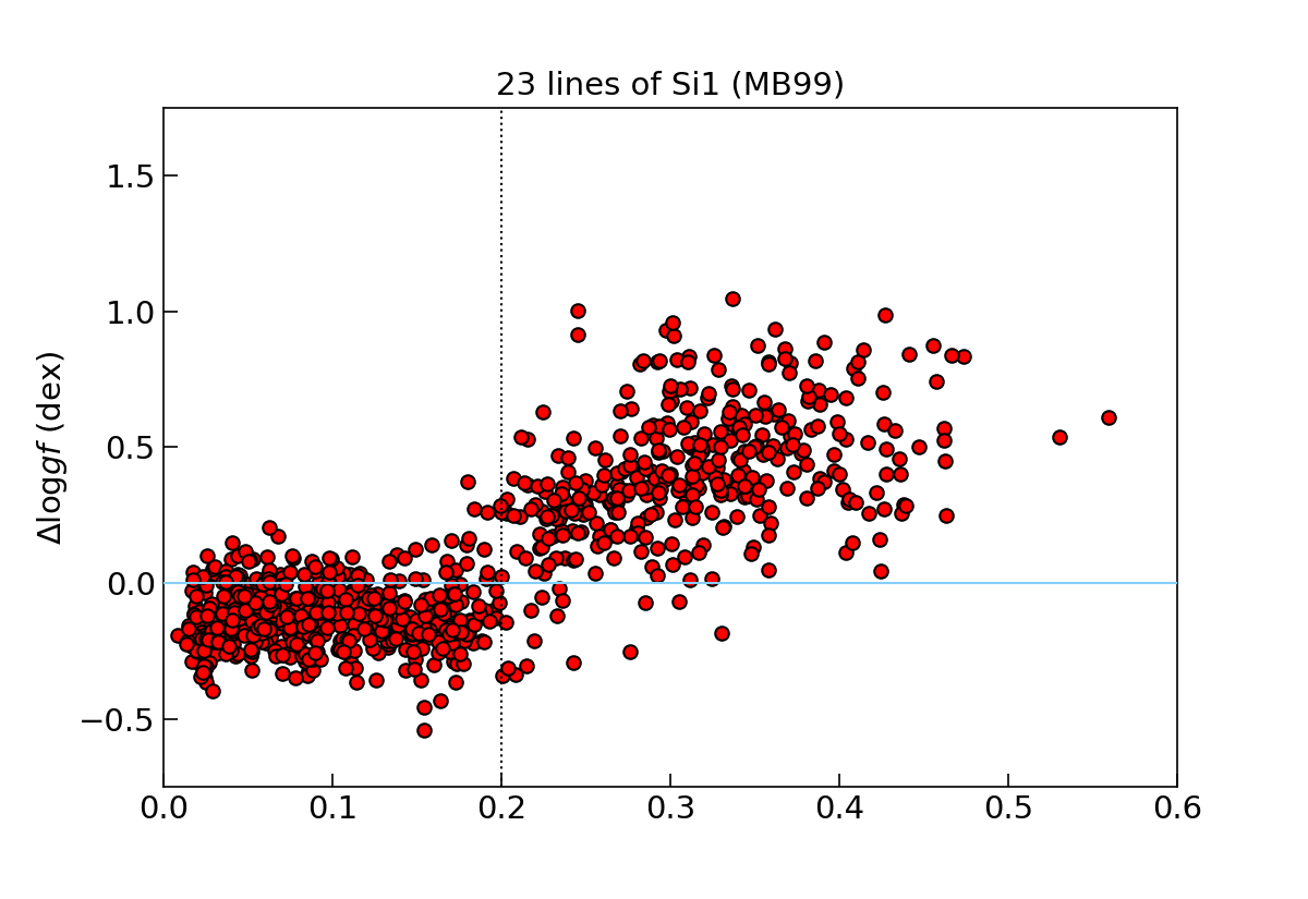
Figure 8: $\Delta{\log gf}_{i}$ for Si i lines from MB99.

5 Abundance Analysis

5.1 Determining microturbulence

In this section, we demonstrate the abundance analysis using the calibrated ${\log gf}$ but without using the stellar parameters estimated with the measurements by Luck (2018). Our analysis starts by estimating ${T_{\mathrm{LDR}}}$ and ${\log g_{\mathrm{trend}}}$ as described in Section  3 and moves on to the determination of $\xi$ before the abundance measurements. The basic idea for determining the microturbulence $\xi$ is to find the condition that makes the abundances from lines of various strengths (non- or less-saturated lines to saturated lines) consistent. Mucciarelli (2011) discussed some methods of determining $\xi$. We measure the abundance from each line as a function of $\xi$. Combining the results for lines with different strengths, we search for $\xi$ with which the abundances show no dependency on line strength. We use the $X$ index:

$$X={\log gf}-EP\cdot\frac{5040}{0.86\,{T_{\mathrm{eff}}}}$$ (6)

as the indicator of line strength (Magain, 1984; Gratton et al., 2006; Kondo et al., 2019). The equivalent width might be a good indicator, but measuring the equivalent width in the observed spectra is not a trivial task as other factors, such as blending, can easily disturb the results. We measure the line depth and use it for rejecting lines deeper than 0.2 in depth, but prefer to use the $X$ indicator here because it is a theoretical value unaffected by observational errors. Then, at each $\xi$, we fit the linear relation,

$${\rm{[Fe/H]}}=aX+b,$$ (7)

to the abundances (${\rm{[Fe/H]}}$) from individual lines as a function of the $X$ index. The slope $a$ changes, usually in a monotonic way, with $\xi$ and we select the $\xi$, one of the $\xi$ grid points with the $0.2\,{\mathrm{km\,s^{-1}}}$ step, that gives the slope closest to zero. Fukue et al. (2021) performed a simulation to find that determining $\xi$ requires at least 20 absorption lines. We use only Fe i lines to estimate $\xi$.

5.2 Abundances with a given microturbulence

Once the microturbulence is obtained, it is relatively simple to derive the abundances making use of an established list of lines (with calibrated ${\log gf}$). For each species, we calculate the weighted mean of ${\rm{[{X}/H]}}_{i}$ from $N$ individual lines that were not rejected, using OCTOMAN to calculate ${\rm{[{X}/H]}}_{i}$ for individual lines and took the weighted mean,

$${\rm{[{X}/H]}}=\left.\sum_{i=1}^{N}\left(w_{i}{\rm{[{X}/H]}}_{i}\right)\right/\sum_{i=1}^{N}w_{i},$$ (8)

where the weights are given by $w_{i}=1/e_{i}^{2}$ and $e_{i}$ is the error in the calibrated ${\log gf}$. We consider the weighted standard deviation,

$$e_{\mathrm{X,1}}=\sqrt{\left.\sum_{i=1}^{N}w_{i}\left({\rm{[{X}/H]}}_{i}-{\rm{[{X}/H]}}\right)^{2}\right/\sum_{i=1}^{N}w_{i}},$$ (9)

as the error of ${\rm{[{X}/H]}}$. Using the standard deviation rather than the standard error (i.e., the standard deviation divided by $\sqrt{N-1}$) is commonly done and recommended by Jofré et al. (2019).

However, Equation (9) would underestimate the uncertainty of the averaged abundance when ${\rm{[{X}/H]}}_{i}$ with a small number of lines get closer, than expected from the statistical errors to each other by coincidence. We consider another indicator of uncertainty,

$$e_{\mathrm{X,2}}=\sqrt{1\left/\sum_{i=1}^{N}w_{i}\right.}~{},$$ (10)

which is given by the error propagation. Then, we take the larger of $e_{\mathrm{X,1}}$ and $e_{\mathrm{X,2}}$ as the error $e_{\mathrm{X}}$ of the derived ${\rm{[{X}/H]}}$. The results of this analysis can be found in Appendix C.

When we have ${\rm{[{X}/H]}}$ estimated with multiple spectra of each Cepheid, we would like to take the mean of phase-by-phase measurements. We calculate the weighted mean using the formula like Equation (8) but with the weights that are determined with the $e_{X}$ of individual phases. The errors are also determined in the same way by taking the larger of the weighted standard deviation (Equation 9) and the propagated error (Equation 10)

5.3 Comparison with the abundances in Luck+18

Using the 46 VALD and 35 MB99 lines with ${\log gf}$ calibrated, we determined the abundances, ${\rm{[{X}/H]}}$, of 9 species. The results are given in Appendix (number). Figures 10 plot ${\rm{[{X}/H]}}$ and the deviations from the literature, Luck (2018), for the calibrators and the validators. For a few species, like Si i (Figure 10), we find very good agreements between our measurements and the literature values ($\sigma\sim 0.07$ dex). Some species, however, show large scatters ($\sigma>0.15$ dex).

Table 4 summarizes how well the abundances we derived agree with the literature values. The mean offsets from the abundance scale of Luck (2018) are not significant for both calibrators and validators. This agreement is expected, at least for the calibrators, because we calibrated ${\log gf}$ based on the abundances of Luck (2018). Yet, the standard deviation is large for some species, in particular, Ca ii and Zn i. The large SDs may be partly attributed to errors in Luck (2018). No significant offsets are found (compared to SD). Looking at Figure 9 for Ca i and Figure 10 for Si i, the abundances of some objects from Luck (2018) seem to show unexpected offsets from other objects; see, e.g., X Cyg for Zn i.

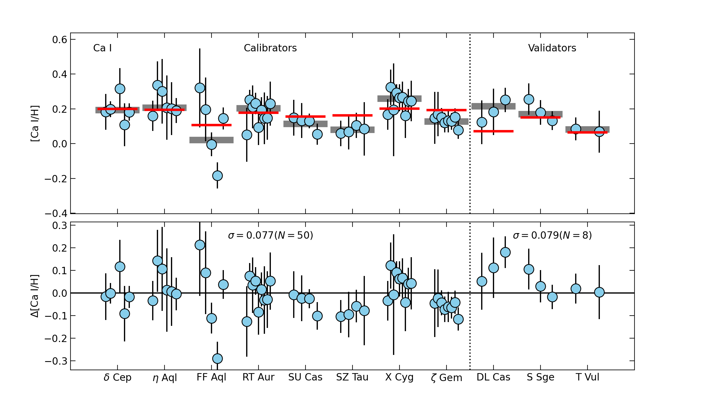
Figure 9: The derived abundances (upper) and the deviations from the literature values (lower) for Ca i.

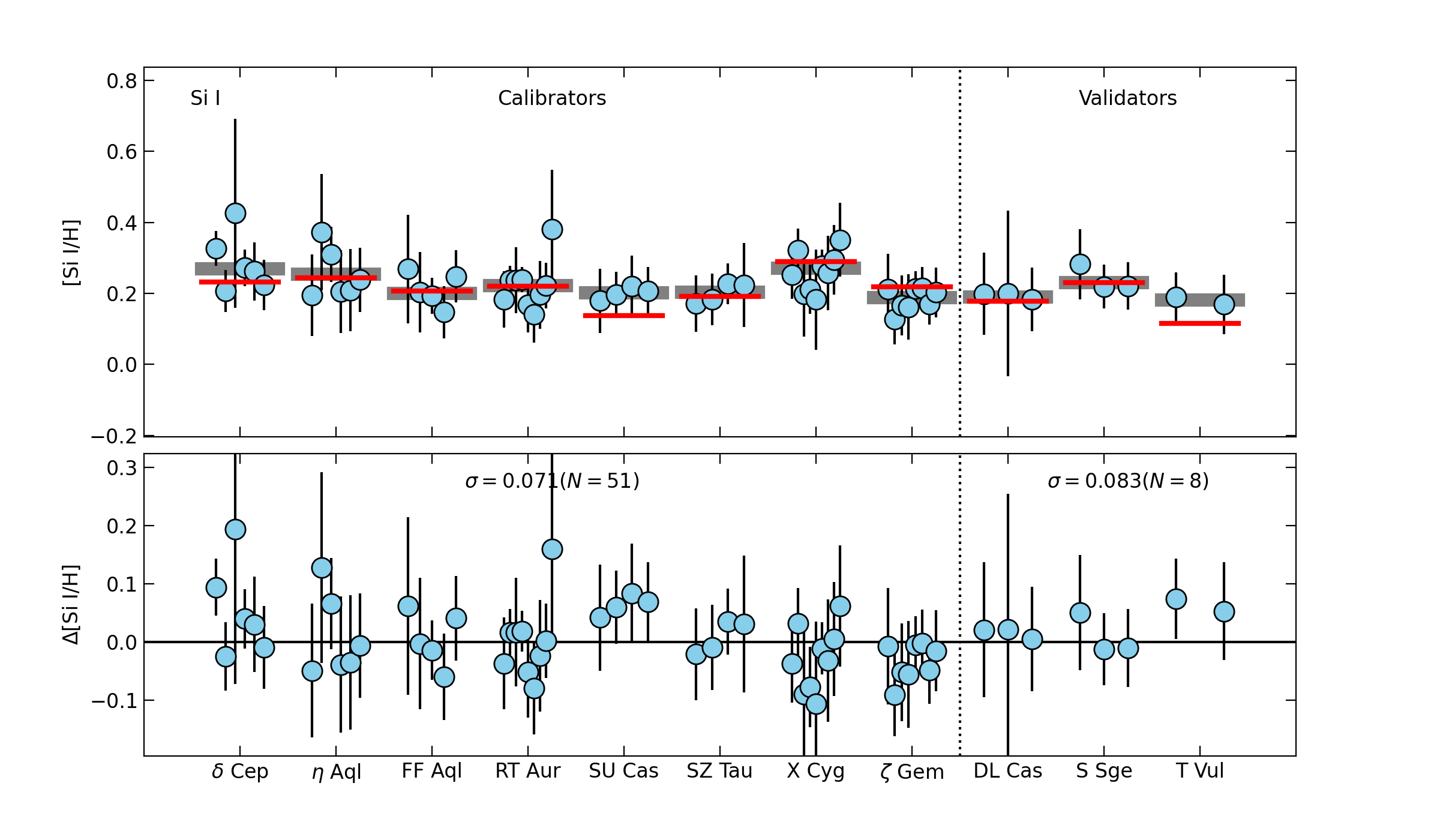
Figure 10: The derived abundances (upper) and the deviations from the literature values (lower) for Si i.

Table 4: Deviations of abundances from Luck (2018) for species other than Fe I

Species	Calibrators			Validators
	Mean	SD	$N$	Mean	SD	$N$
	(dex)	(dex)		(dex)	(dex)
$\mathrm{Si\,I}$	$0.003$	0.071	51	$0.003$	0.083	8
$\mathrm{P\,I}$	$-0.003$	0.064	51	$-0.003$	0.065	8
$\mathrm{S\,I}$	$-0.029$	0.100	51	$-0.029$	0.108	8
$\mathrm{Ca\,I}$	$-0.022$	0.077	50	$-0.022$	0.079	8
$\mathrm{Ca\,II}$	$-0.051$	0.268	32	$-0.051$	0.209	4
$\mathrm{Fe\,II}$	$-0.006$	0.072	51	$-0.006$	0.090	8
$\mathrm{Zn\,I}$	$-0.080$	0.179	37	$-0.080$	0.129	4
$\mathrm{Y\,II}$	$-0.003$	0.114	48	$-0.003$	0.090	8
$\mathrm{Dy\,II}$	$-0.078$	0.176	14	$-0.078$	0.176	4

6 Concluding remarks

We have successfully established a list of elements in neutral and ionized state of nine species (including Fe) that are useful for measuring the abundances of classical Cepheids. We calibrated the ${\log gf}$ of these lines by comparing our measurements with the abundances of eight calibrators in Luck (2018), and thus-calibrated ${\log gf}$ gives the abundances of the validators consistent with those in Luck (2018). The precision for a few species is as high as the abundance analysis with optical spectra. A few points are worth further consideration.

(1) The method described in this work for obtaining effective temperatures using the LDR relations leads to high precision ($\leq$ 100 K) except for some cases with high ${T_{\mathrm{eff}}}$ ($\geq$ 6000 K) and/or low S/N ($\leq$ 150). This gives a rough guide to future observers; YJ - band spectra with S/N $\sim$ 100 or higher would allow precise abundance measurements, while warmer Cepheids would require higher S/N.

(2) The impact of microturbulence on the strength of each line is known to be affected by the line strength. In the determination of ${\log gf}$ of a given species, a question arises as to whether it is appropriate to use $\xi$ obtained solely with Fe i lines. We have observed so that the utilization of stronger lines, such as those of Silicon or Strontium, may also impact the resulting $\xi$, providing evidence that $\xi$ changes along the atmosphere of Cepheids at different $\tau$. This phenomenon was initially reported by Takeda & Sadakane (1997) in an HB star, and later on in RR Lyrae by Takeda et al. (2006); Kolenberg et al. (2010); Fossati et al. (2014). This suggests that $\xi$ increases with height in the atmosphere of RR Lyrae stars, as reported in Fossati et al. (2014). Additionally, it is recommended that a specific $\xi$ be applied to lines with specific strength to avoid erroneous abundance estimates. Considering the depth-dependent $\xi$ could make it possible to include such strong lines, but we have no set of atmosphere models with depth-dependent $\xi$ for Cepheids in which the turbulent velocity field may well be different from static stars. Therefore, in this paper, we rejected lines stronger than 0.2 and focused on weaker lines and we suggest to avoid such strong lines in the future abundance analyses.

(3) Phosphorus, an odd-Z ($Z=15$) element, whose isotope belongs to the same group as Nitrogen is believed to have been produced during the C and Ne burning. It is one of the most fundamental life-bearing elements dominated by macromolecules composed mainly of Carbon that are present in every single organism formed by cells. Each contains membranes and inner organelles whose primary component is a molecule denominated Phospholipid (a.k.a. phosphatides) which is a class of lipid whose molecule is formed by a hydrophilic head where the phosphate group is located as well as two hydrophobic tails. Moreover, from Biology, we know that when DNA is synthesized, a molecule called adenosine triphosphate (ATP) brings energy to the whole DNA structure, by keeping it together, as a superglue. Phosphorus, chemically-wise, has been surprisingly skipped for years. An example of this is that prior 2011, with the study of Caffau et al. (2007), P was barely analyzed in stars. A possible cause for this sort of dodging was raised back in the early 1930’s by Struve (1930) who found that no neutral P was available in spectra of stars whose spectral type ranged from F-K. Though, it was acknowledged that Phosphorus ions might be visible in other kinds of stars or other regimes (Maas et al., 2020; Naghma et al., 2018), such as P ii, P ii, P iii, P iv observable in UV spectra. A handful of studies have been done on stars after the study of Caffau et al. (2007) which first suggested using the high-excitation P i lines in multiplet at 1051-1068 nm. Different authors have focused their attention on various other targets of interest: such as Hubrig et al. (2009) obtained P i abundance of HB stars in globular clusters. Meléndez et al. (2009) investigated the P i abundances of a handful of solar twins. Sbordone et al. (2009) suggested that Sulphur could have been produced by proton capture on P, leading to a debate on how possible it is to create the amount of S found there as a product of P when P was never measured on stars in that globular cluster. The work on stars in our galaxy was first reported with the P abundance on 22 MS (main sequence) stars Caffau et al. (2005), stars in the galactic disk Caffau et al. (2011), and dwarf stars (Caffau et al., 2016). Discussions on biological and geological implications can be found, e.g., in Hinkel et al. (2020). We detected more lines of P i present in our NIR spectra observed with WINERED whose abundances were also measured. None of the aforementioned studies have included Cepheids. Our study on the P abundance is probably the first to be performed on stars as hot and variable as Cepheids. We confirmed ten P i lines in our spectra of which 9 had their ${\log gf}$ values calibrated.

(4) From the works of Luck (2018) on hundreds of Cepheids, which itself included our sample of Calibrators and Validators, the abundances of a handful of elements were provided. Our estimates of chemical abundances are in agreement with the abundance gradient found by Luck (2018) and prove that we can use spectra in the $YJ$ bands to take the study of the Galactic Chemistry to the next level by including the interstellar-hidden Cepheids that can be observed in the infrared only.

Appendix A Stellar Parameters

Here, we provide the derived stellar parameters (${T_{\mathrm{eff}}}$ and ${\log g}$) for each of the targets at each of their obtained phases.

Table 5: Stellar Parameters derived for the calibrators sample.

ID	Phase	${T_{\mathrm{LDR}}}$	$e_{{T_{\mathrm{LDR}}}}$	$N_{{T_{\mathrm{LDR}}}}$	${\log g_{\mathrm{LDR}}}$	$e_{\log g_{\mathrm{LDR}}}$	$N_{{\log g_{\mathrm{LDR}}}}$	${\log g_{\mathrm{trend}}}$	$e_{{\log g_{\mathrm{trend}}}}$
$\delta$ Cep	0.119	6158.858	109.492	9	1.995	0.129	10	2.079	0.119
	0.178	5974.720	95.670	10	2.177	0.163	8	1.993	0.117
	0.556	5564.740	52.993	12	1.974	0.118	9	1.793	0.111
	0.672	5460.668	78.134	11	1.611	0.140	10	1.740	0.115
	0.711	5530.576	41.254	11	1.812	0.104	9	1.776	0.110
	0.897	6305.770	292.722	3	2.310	0.194	6	2.145	0.170
$\eta$ Aql	0.174	5851.384	86.724	11	1.755	0.145	8	1.836	0.116
	0.216	5846.917	75.231	10	1.757	0.106	9	1.834	0.114
	0.395	5674.762	90.609	11	2.070	0.161	9	1.750	0.117
	0.700	5304.119	41.614	11	1.475	0.107	9	1.560	0.110
	0.743	5357.368	145.628	8	1.439	0.235	6	1.588	0.132
	0.887	5886.794	134.170	9	1.774	0.147	8	1.853	0.126
FF Aql	0.105	6257.612	66.101	9	2.225	0.102	10	2.185	0.112
	0.594	5918.142	148.542	6	2.067	0.172	7	2.028	0.129
	0.627	6156.364	62.646	12	2.143	0.105	10	2.139	0.112
	0.737	6299.516	54.178	10	2.294	0.097	10	2.204	0.111
	0.823	6155.288	154.563	9	1.774	0.112	10	2.138	0.129
RT Aur	0.149	6303.853	168.488	6	2.207	0.151	8	2.267	0.132
	0.155	6382.660	81.993	9	2.385	0.109	10	2.302	0.114
	0.252	6069.138	47.748	12	2.136	0.098	10	2.160	0.110
	0.341	5851.989	44.895	12	1.940	0.097	10	2.057	0.110
	0.422	5711.910	50.499	11	1.917	0.102	10	1.989	0.111
	0.492	5680.734	45.042	12	1.760	0.100	10	1.974	0.110
	0.620	5667.429	50.531	8	1.927	0.123	7	1.967	0.111
	0.776	5737.308	81.643	12	1.913	0.159	7	2.001	0.115
	0.920	6206.251	67.663	9	2.166	0.103	10	2.223	0.112
SU Cas	0.108	6341.471	98.568	8	2.193	0.114	10	2.502	0.117
	0.150	6420.494	123.257	7	2.305	0.121	10	2.537	0.121
	0.546	6103.989	75.763	11	2.261	0.112	10	2.394	0.114
SZ Tau	0.502	5813.069	82.707	12	1.953	0.143	9	2.095	0.115
	0.639	5799.423	56.040	12	1.860	0.112	9	2.089	0.111
	0.772	6114.620	128.669	7	2.334	0.142	9	2.238	0.123
	0.870	6099.724	87.401	6	2.034	0.111	9	2.231	0.115
X Cyg	0.030	6006.767	61.034	11	1.794	0.114	8	1.632	0.112
	0.103	5628.700	48.255	10	1.404	0.098	10	1.449	0.111
	0.353	5058.509	39.302	11	1.385	0.117	10	1.149	0.110
	0.408	4912.173	61.398	9	0.992	0.268	8	1.066	0.114
	0.582	4716.821	51.199	10	0.739	0.466	5	0.952	0.112
	0.408	4912.173	61.398	9	0.992	0.268	8	1.066	0.114

ID	Phase	${T_{\mathrm{LDR}}}$	$e_{{T_{\mathrm{LDR}}}}$	$N_{{T_{\mathrm{LDR}}}}$	${\log g_{\mathrm{LDR}}}$	$e_{\log g_{\mathrm{LDR}}}$	$N_{{\log g_{\mathrm{LDR}}}}$	${\log g_{\mathrm{trend}}}$	$e_{{\log g_{\mathrm{trend}}}}$
X Cyg	0.582	4716.821	51.199	10	0.739	0.466	5	0.952	0.112
	0.606	4726.672	42.517	11	0.759	0.208	4	0.958	0.111
	0.685	4852.158	51.921	10	1.191	0.159	5	1.031	0.112
	0.760	5101.901	70.059	9	1.080	0.233	2	1.173	0.115
	0.880	5383.506	39.783	12	1.467	0.106	9	1.324	0.110
$\zeta$ Gem	0.028	5803.001	41.689	10	1.696	0.094	10	1.696	0.110
	0.133	5636.552	41.616	12	1.579	0.102	9	1.614	0.110
	0.200	5488.495	42.429	12	1.483	0.099	10	1.540	0.110
	0.534	5246.328	36.864	12	1.365	0.100	9	1.412	0.110
	0.626	5509.257	44.747	10	1.740	0.113	8	1.550	0.110
	0.645	5442.997	38.323	11	1.433	0.101	9	1.516	0.110
	0.791	5706.932	54.991	12	1.671	0.110	9	1.649	0.111
	0.923	5711.450	43.379	10	1.508	0.095	10	1.652	0.110

Table 6: Stellar Parameters derived for the validators sample.

ID	Phase	${T_{\mathrm{LDR}}}$	$e_{{T_{\mathrm{LDR}}}}$	$N_{{T_{\mathrm{LDR}}}}$	${\log g_{\mathrm{LDR}}}$	$e_{\log g_{\mathrm{LDR}}}$	$N_{{\log g_{\mathrm{LDR}}}}$	${\log g_{\mathrm{trend}}}$	$e_{{\log g_{\mathrm{trend}}}}$
DL Cas	0.219	5855.625	94.278	8	1.924	0.124	9	1.802	0.117
	0.604	5310.473	83.805	8	1.550	0.158	7	1.527	0.117
	0.743	5422.091	107.744	8	1.662	0.229	3	1.585	0.122
S Sge	0.119	5996.566	71.749	12	1.968	0.115	10	1.853	0.113
	0.520	5342.743	39.696	12	1.426	0.098	10	1.528	0.110
	0.940	6097.361	107.231	10	1.823	0.134	9	1.900	0.119
T Vul	0.138	6131.199	102.707	9	2.104	0.135	8	2.130	0.118
	0.293	5798.716	52.616	12	1.798	0.104	10	1.973	0.111

Appendix B Calibrated log gf for Fe I and species lines

Here, we include the results of our method for calculating the oscillator strengths (${\log gf}$ values) by following the procedure stated in Section 4.3.

Table 7: Calibration of $\log gf$ of Fe i lines

$\lambda_{\mathrm{air}}$	EP	$\log gf_{\mathrm{VALD}}$ (dex)		$\log gf_{\mathrm{MB99}}$ (dex)
(Å)	(eV)	old	new (SD, $N$)	old	new (SD, $N$)
9800.3075	5.0856	$-0.453$	$-0.715$ (0.139, 21)	—	—
9811.5041	5.0117	$-1.362$	$-1.487$ (0.098, 33)	—	—
9861.7337	5.0638	$-0.142$	$-0.623$ (0.084, 39)	—	—
9868.1857	5.0856	$-0.979$	$-0.885$ (0.075, 39)	—	—
9944.2065	5.0117	$-1.338$	$-1.476$ (0.126, 22)	—	—
9980.4629	5.0331	$-1.379$	$-1.546$ (0.093, 43)	—	—
10041.472	5.0117	$-1.772$	$-1.856$ (0.175, 20)	$-1.840$	$-1.868$ (0.169, 26)
10065.045	4.8349	$-0.289$	$-0.600$ (0.129, 31)	$-0.570$	$-0.597$ (0.132, 29)
10114.020	2.7600	—	—	$-3.760$	$-3.711$ (0.147, 23)
10145.561	4.7955	$-0.177$	$-0.349$ (0.109, 47)	$-0.410$	$-0.382$ (0.105, 48)
10155.162	2.1759	$-4.226$	$-4.611$ (0.162, 26)	$-4.360$	$-4.518$ (0.091, 38)
10167.468	2.1979	$-4.117$	$-4.350$ (0.103, 41)	$-4.260$	$-4.380$ (0.104, 39)
10195.105	2.7275	$-3.580$	$-3.765$ (0.109, 43)	$-3.630$	$-3.781$ (0.109, 46)
10216.313	4.7331	$-0.063$	$-0.226$ (0.126, 49)	$-0.290$	$-0.232$ (0.137, 50)
10218.408	3.0713	$-2.760$	$-3.014$ (0.101, 48)	$-2.930$	$-3.044$ (0.093, 49)
10227.994	6.1189	$-0.354$	$-0.299$ (0.093, 38)	—	—
10265.217	2.2227	$-4.537$	$-4.750$ (0.096, 23)	—	—
10340.885	2.1979	$-3.577$	$-3.789$ (0.096, 48)	$-3.650$	$-3.814$ (0.086, 49)
10347.965	5.3933	$-0.551$	$-0.839$ (0.058, 48)	$-0.820$	$-0.894$ (0.051, 50)
10353.804	5.3933	$-0.819$	$-1.098$ (0.071, 48)	$-1.090$	$-1.108$ (0.070, 50)
10395.794	2.1759	$-3.393$	$-3.455$ (0.076, 28)	$-3.420$	$-3.570$ (0.118, 36)
10469.652	3.8835	$-1.184$	$-1.736$ (0.098, 39)	$-1.370$	$-1.758$ (0.104, 37)
10532.234	3.9286	$-1.480$	$-1.918$ (0.076, 51)	$-1.760$	$-1.960$ (0.066, 50)
10535.709	6.2057	$-0.108$	$-0.219$ (0.075, 50)	—	—
10577.139	3.3014	$-3.136$	$-3.452$ (0.123, 40)	$-3.280$	$-3.519$ (0.137, 41)
10611.686	6.1692	$0.021$	$-0.090$ (0.066, 51)	$-0.090$	$-0.110$ (0.065, 51)
10616.721	3.2671	$-3.127$	$-3.536$ (0.093, 22)	$-3.340$	$-3.537$ (0.110, 45)
10674.070	6.1692	$-0.466$	$-0.586$ (0.196, 22)	—	—
10725.185	3.6398	$-2.763$	$-2.937$ (0.123, 23)	$-2.980$	$-2.948$ (0.125, 22)
10753.004	3.9597	$-1.845$	$-2.217$ (0.097, 26)	$-2.140$	$-2.214$ (0.094, 27)
10818.274	3.9597	$-1.948$	$-2.292$ (0.086, 47)	$-2.230$	$-2.325$ (0.095, 41)
10849.460	5.5400	—	—	$-0.730$	$-0.828$ (0.083, 44)
10863.518	4.7331	$-0.895$	$-1.032$ (0.093, 36)	$-1.060$	$-1.135$ (0.075, 49)
12053.082	4.5585	$-1.543$	$-1.767$ (0.136, 44)	$-1.750$	$-1.803$ (0.128, 44)
12119.494	4.5931	$-1.635$	$-1.977$ (0.180, 20)	—	—
12190.098	3.6352	$-2.330$	$-2.748$ (0.131, 38)	$-2.750$	$-2.823$ (0.124, 41)
12283.298	6.1692	$-0.537$	$-0.651$ (0.180, 20)	$-0.610$	$-0.584$ (0.144, 22)
12342.916	4.6382	$-1.463$	$-1.703$ (0.122, 42)	$-1.680$	$-1.690$ (0.135, 33)
12556.996	2.2786	$-3.626$	$-4.110$ (0.128, 37)	$-4.070$	$-4.147$ (0.144, 32)
12638.703	4.5585	$-0.783$	$-1.153$ (0.165, 35)	$-1.000$	$-1.164$ (0.161, 34)
12648.741	4.6070	$-1.140$	$-1.325$ (0.153, 33)	$-1.320$	$-1.364$ (0.158, 35)
12789.470	5.0100	—	—	$-1.920$	$-1.704$ (0.148, 23)
12807.152	3.6398	$-2.452$	$-2.710$ (0.166, 20)	$-2.760$	$-2.728$ (0.122, 26)
12879.766	2.2786	$-3.458$	$-3.686$ (0.115, 31)	$-3.610$	$-3.714$ (0.103, 33)
13006.684	2.9904	$-3.744$	$-3.493$ (0.142, 20)	—	—

Table 7: Calibration of $\log gf$ of Fe i lines—continued.

Table 8: Calibration of $\log gf$ of lines other than $\mathrm{Fe\,I}$

	$\lambda_{\mathrm{air}}$	EP	$\log gf_{\mathrm{VALD}}$ (dex)		$\log gf_{\mathrm{MB99}}$ (dex)
	(Å)	(eV)	old	new (SD, $N$)	old	new (SD, $N$)
Si i	10068.329	6.099	$-1.318$	$-1.566$ (0.071, 37)	$-1.400$	$-1.564$ (0.070, 39)
Si i	10288.944	4.920	$-1.511$	$-1.851$ (0.078, 51)	$-1.710$	$-1.885$ (0.074, 50)
Si i	10301.410	6.100	—	—	$-1.830$	$-1.946$ (0.121, 31)
Si i	10313.197	6.399	$-0.886$	$-1.460$ (0.125, 31)	—	—
Si i	10407.037	6.616	$-0.597$	$-0.937$ (0.072, 48)	$-0.770$	$-0.891$ (0.074, 48)
Si i	10414.913	6.619	$-1.137$	$-1.579$ (0.113, 45)	$-1.380$	$-1.563$ (0.095, 46)
Si i	10582.160	6.223	$-1.169$	$-1.218$ (0.088, 21)	—	—
Si i	10784.562	5.964	$-0.839$	$-0.838$ (0.088, 45)	$-0.720$	$-0.886$ (0.076, 45)
Si i	10796.106	6.181	$-1.266$	$-1.628$ (0.104, 40)	$-1.490$	$-1.561$ (0.123, 39)
Si i	10882.809	5.984	$-0.815$	$-0.812$ (0.085, 39)	$-0.620$	$-0.789$ (0.077, 41)
Si i	12110.659	6.616	$-0.136$	$-0.411$ (0.147, 23)	—	—
Si i	12175.733	6.619	$-0.855$	$-1.061$ (0.106, 33)	$-0.970$	$-1.052$ (0.116, 39)
Si i	12178.339	6.269	$-1.100$	$-1.161$ (0.122, 45)	$-1.140$	$-1.179$ (0.124, 45)
Si i	12390.154	5.082	$-1.767$	$-1.977$ (0.098, 47)	$-1.930$	$-2.006$ (0.096, 48)
Si i	12395.832	4.954	$-1.644$	$-1.871$ (0.084, 47)	$-1.820$	$-1.874$ (0.085, 48)
Si i	12583.924	6.616	$-0.462$	$-0.736$ (0.145, 37)	$-0.620$	$-0.751$ (0.124, 36)
P i	9796.8280	6.985	$0.270$	$0.338$ (0.104, 38)	—	—
P i	9903.6710	7.176	$-0.300$	$-0.322$ (0.142, 24)	—	—
P i	10084.277	7.213	$0.140$	$0.202$ (0.129, 30)	$-0.070$	$0.141$ (0.140, 36)
P i	10204.700	7.210	—	—	$-0.590$	$-0.543$ (0.115, 24)
P i	10511.588	6.936	$-0.130$	$-0.192$ (0.116, 42)	$-0.220$	$-0.195$ (0.110, 42)
P i	10529.524	6.954	$0.240$	$0.432$ (0.055, 46)	$0.140$	$0.360$ (0.067, 46)
P i	10581.577	6.985	$0.450$	$0.660$ (0.132, 44)	$0.360$	$0.678$ (0.121, 45)
P i	10596.903	6.936	$-0.210$	$-0.005$ (0.075, 49)	$-0.280$	$-0.074$ (0.096, 49)
P i	10813.141	6.985	$-0.410$	$-0.395$ (0.128, 33)	$-0.440$	$-0.409$ (0.153, 36)
S i	10635.970	8.580	—	—	$0.380$	$0.478$ (0.116, 49)
S i	10821.180	0.000	$-8.607$	$-8.762$ (0.074, 32)	$-8.550$	$-8.743$ (0.101, 39)
Ca i	10343.819	2.932	$-0.300$	$-0.446$ (0.106, 50)	$-0.400$	$-0.439$ (0.105, 49)
Ca i	10516.140	4.740	—	—	$-0.520$	$-0.765$ (0.160, 33)
Ca i	10791.450	4.740	—	—	$-0.680$	$-0.740$ (0.132, 21)
Ca i	10838.970	4.878	$0.238$	$-0.141$ (0.113, 44)	$0.030$	$-0.140$ (0.106, 43)
Ca i	10846.790	4.740	—	—	$-0.640$	$-0.565$ (0.086, 39)
Ca i	11955.955	4.131	$-0.849$	$-1.065$ (0.180, 22)	$-0.910$	$-1.060$ (0.183, 21)
Ca i	12105.840	4.550	—	—	$-0.540$	$-0.726$ (0.168, 24)
Ca i	13033.554	4.441	$-0.064$	$-0.415$ (0.159, 32)	$-0.310$	$-0.379$ (0.164, 34)
Ca i	13134.942	4.451	$0.085$	$-0.181$ (0.198, 22)	$-0.140$	$-0.185$ (0.198, 22)
Ca ii	9854.7590	7.505	$-0.205$	$-0.277$ (0.134, 32)	—	—
Fe ii	9956.3220	5.484	$-2.985$	$-3.017$ (0.130, 35)	—	—
Fe ii	9997.5980	5.484	$-1.867$	$-1.721$ (0.164, 40)	—	—
Fe ii	10173.515	5.511	$-2.736$	$-2.805$ (0.103, 43)	—	—
Fe ii	10189.060	6.729	$-2.141$	$-2.225$ (0.127, 32)	—	—
Fe ii	10245.556	6.730	$-2.057$	$-1.865$ (0.198, 28)	—	—
Fe ii	10332.928	6.729	$-1.968$	$-1.965$ (0.100, 37)	—	—
Fe ii	10366.167	6.724	$-1.825$	$-1.860$ (0.114, 47)	—	—
Fe ii	10490.945	5.549	$-2.985$	$-2.915$ (0.101, 42)	—	—
Fe ii	10501.503	5.548	$-2.086$	$-1.975$ (0.086, 50)	—	—
Fe ii	10525.149	5.553	$-2.958$	$-2.938$ (0.092, 46)	—	—
Fe ii	10862.652	5.589	$-2.199$	$-2.327$ (0.107, 26)	—	—
Fe ii	10871.626	5.589	$-3.098$	$-2.974$ (0.111, 24)	—	—
Zn i	13053.600	6.655	$0.340$	$0.329$ (0.176, 35)	$0.130$	$0.320$ (0.163, 32)
Y ii	10105.520	1.721	$-1.890$	$-1.672$ (0.126, 34)	$-1.890$	$-1.627$ (0.130, 35)
Y ii	10186.460	1.839	—	—	$-1.970$	$-2.215$ (0.148, 25)
Y ii	10245.220	1.738	$-1.820$	$-2.167$ (0.191, 36)	$-1.910$	$-2.246$ (0.230, 25)
Y ii	10329.700	1.748	$-1.760$	$-1.877$ (0.121, 24)	$-1.710$	$-1.885$ (0.125, 34)
Y ii	10605.150	1.738	$-1.960$	$-1.844$ (0.118, 43)	$-1.890$	$-1.844$ (0.119, 41)
Dy ii	10523.390	1.946	$-0.450$	$-0.357$ (0.176, 21)	—	—

Table 8: Calibration of $\log gf$ of lines other than $\mathrm{Fe\,I}$—continued.

Appendix C Derived abundances for the calibrators and validators sample.

Table 9: Derived microturbulence and Fe i abundance

Cepheid	Date (Phase)	$T_{\mathrm{LDR}}$	$\log g_{\mathrm{rel}}$	$\xi$	[Fe/H] (SD, $N$)
		(K)	(dex)	(km s-1)	(dex)
Calibrators
$\delta$ Cep	20131202 (0.119)	6159	2.08	2.40	$0.10$ (0.14, 52)
	20131205 (0.672)	5461	1.74	3.40	$0.04$ (0.14, 53)
	20150806 (0.178)	5975	1.99	3.00	$0.14$ (0.17, 35)
	20150808 (0.556)	5565	1.79	3.40	$0.04$ (0.13, 59)
	20150815 (0.897)	6306	2.14	3.60	$0.01$ (0.17, 35)
	20151023 (0.711)	5531	1.78	3.60	$0.02$ (0.13, 61)
$\eta$ Aql	20140916 (0.743)	5357	1.59	4.20	$0.03$ (0.15, 47)
	20150806 (0.887)	5887	1.85	3.00	$0.14$ (0.17, 35)
	20150808 (0.174)	5851	1.84	2.80	$0.15$ (0.15, 51)
	20160321 (0.700)	5304	1.56	4.20	$-0.04$ (0.15, 42)
	20160326 (0.395)	5675	1.75	3.00	$0.06$ (0.16, 52)
	20160514 (0.216)	5847	1.83	2.40	$0.17$ (0.15, 44)
FF Aql	20150806 (0.594)	5918	2.03	3.00	$0.02$ (0.16, 37)
	20150807 (0.823)	6155	2.14	3.40	$-0.08$ (0.15, 43)
	20160317 (0.737)	6300	2.20	3.40	$-0.02$ (0.14, 52)
	20160321 (0.627)	6156	2.14	5.20	$-0.13$ (0.15, 46)
	20160419 (0.105)	6258	2.18	3.20	$0.08$ (0.13, 57)
RT Aur	20140123 (0.920)	6206	2.22	3.20	$-0.05$ (0.13, 57)
	20151028 (0.422)	5712	1.99	2.20	$0.07$ (0.13, 62)
	20160216 (0.149)	6304	2.27	2.20	$0.13$ (0.16, 38)
	20160228 (0.341)	5852	2.06	1.80	$0.10$ (0.12, 66)
	20160307 (0.492)	5681	1.97	2.40	$0.10$ (0.13, 61)
	20160315 (0.620)	5667	1.97	3.00	$0.02$ (0.12, 65)
	20160317 (0.155)	6383	2.30	2.80	$0.12$ (0.14, 54)
	20160321 (0.252)	6069	2.16	2.40	$0.07$ (0.13, 61)
	20160323 (0.776)	5737	2.00	3.60	$-0.01$ (0.12, 65)
SU Cas	20150815 (0.014)	nan	nan	1.80	$0.04$ (0.17, 34)
	20160312 (0.546)	6104	2.39	2.20	$-0.07$ (0.13, 57)
	20160315 (0.108)	6341	2.50	1.80	$0.01$ (0.15, 44)
	20160317 (0.150)	6420	2.54	2.20	$-0.04$ (0.14, 49)
SZ Tau	20140124 (0.870)	6100	2.23	3.40	$-0.07$ (0.15, 46)
	20160218 (0.639)	5799	2.09	3.00	$-0.06$ (0.13, 57)
	20160317 (0.502)	5813	2.10	2.40	$-0.02$ (0.13, 62)
	20160321 (0.772)	6115	2.24	2.40	$-0.05$ (0.16, 48)
X Cyg	20140830 (0.606)	4727	0.96	4.00	$0.07$ (0.14, 49)
	20140915 (0.582)	4717	0.95	3.60	$0.11$ (0.14, 54)
	20140918 (0.760)	5102	1.17	5.80	$0.02$ (0.18, 58)
	20141015 (0.408)	4912	1.07	3.80	$0.08$ (0.13, 60)
	20150725 (0.685)	4852	1.03	4.60	$0.12$ (0.15, 46)
	20151026 (0.353)	5059	1.15	2.40	$0.07$ (0.14, 49)
	20160317 (0.103)	5629	1.45	3.20	$0.04$ (0.13, 62)
	20160504 (0.030)	6007	1.63	3.40	$0.10$ (0.13, 57)
	20160518 (0.880)	5384	1.32	3.60	$0.26$ (0.13, 59)
$\zeta$ Gem	20130222 (0.534)	5246	1.41	2.80	$0.01$ (0.12, 65)
	20130223 (0.645)	5443	1.52	4.60	$-0.06$ (0.13, 56)
	20130227 (0.028)	5803	1.70	3.20	$-0.13$ (0.14, 55)
	20131129 (0.133)	5637	1.61	3.60	$-0.04$ (0.12, 69)
	20160217 (0.923)	5711	1.65	2.60	$0.00$ (0.15, 47)
	20160307 (0.791)	5707	1.65	3.40	$0.03$ (0.14, 53)
	20160501 (0.200)	5488	1.54	3.60	$0.04$ (0.13, 58)
	20171204 (0.626)	5509	1.55	4.60	$-0.02$ (0.15, 44)
DL Cas	20150731 (0.743)	5422	1.59	3.20	$-0.10$ (0.15, 43)
	20150807 (0.604)	5310	1.53	3.80	$-0.12$ (0.14, 58)
	20151023 (0.219)	5856	1.80	3.20	$-0.00$ (0.12, 65)
S Sge	20151026 (0.940)	6097	1.90	3.00	$0.03$ (0.16, 40)
	20160321 (0.520)	5343	1.53	3.40	$-0.03$ (0.13, 59)
	20160326 (0.119)	5997	1.85	3.60	$0.03$ (0.14, 52)
T Vul	20150808 (0.138)	6131	2.13	2.80	$-0.01$ (0.15, 47)
	20160514 (0.293)	5799	1.97	2.20	$-0.04$ (0.14, 52)

Table 9: Derived microturbulence and Fe i abundance—continued.

Table 10: Abundances other than $\mathrm{Fe\,I}$ (Part 1)

Cepheid	Date	$\mathrm{Si\,I}$	$\mathrm{P\,I}$	$\mathrm{S\,I}$
$\delta$ Cep	20131202	$0.33$ (0.08, 19)	$0.11$ (0.05, 10)	$0.32$ (0.05, 3)
	20131205	$0.21$ (0.04, 22)	$-0.01$ (0.05, 9)	$0.20$ (0.06, 3)
	20150806	$0.29$ (0.12, 12)	$0.10$ (0.04, 9)	$0.25$ (0.12, 1)
	20150808	$0.24$ (0.05, 16)	$0.00$ (0.05, 11)	$0.27$ (0.08, 3)
	20150815	$0.25$ (0.10, 21)	$-0.01$ (0.04, 12)	$-0.00$ (0.27, 3)
	20151023	$0.19$ (0.04, 24)	$-0.03$ (0.03, 12)	$0.15$ (0.05, 3)
$\eta$ Aql	20140916	$0.18$ (0.18, 13)	$0.08$ (0.20, 9)	$0.52$ (0.18, 2)
	20150806	$0.33$ (0.13, 19)	$0.19$ (0.16, 11)	$0.14$ (0.11, 2)
	20150808	$0.30$ (0.11, 26)	$0.12$ (0.11, 14)	$0.35$ (0.10, 3)
	20160321	$0.12$ (0.08, 22)	$0.02$ (0.12, 11)	$0.27$ (0.17, 3)
	20160326	$0.28$ (0.08, 26)	$0.07$ (0.07, 12)	$0.34$ (0.12, 3)
	20160514	$0.32$ (0.06, 22)	$0.15$ (0.08, 10)	$0.39$ (0.05, 3)
FF Aql	20150806	$0.13$ (0.11, 15)	$0.05$ (0.10, 9)	$0.29$ (0.12, 1)
	20150807	$0.19$ (0.12, 22)	$0.06$ (0.07, 8)	$0.36$ (0.12, 1)
	20160317	$0.21$ (0.07, 25)	$0.06$ (0.03, 11)	$0.16$ (0.23, 2)
	20160321	$0.10$ (0.09, 23)	$-0.01$ (0.08, 13)	$0.17$ (0.08, 3)
	20160419	$0.24$ (0.07, 25)	$0.05$ (0.06, 13)	$0.29$ (0.05, 3)
RT Aur	20140123	$0.19$ (0.07, 21)	$0.03$ (0.04, 12)	$0.36$ (0.12, 1)
	20151028	$0.27$ (0.06, 26)	$0.08$ (0.04, 12)	$0.31$ (0.06, 3)
	20160216	$0.30$ (0.11, 27)	$0.09$ (0.05, 14)	$0.44$ (0.12, 1)
	20160228	$0.31$ (0.06, 25)	$0.07$ (0.07, 15)	$0.29$ (0.05, 3)
	20160307	$0.21$ (0.07, 25)	$0.05$ (0.06, 12)	$0.22$ (0.05, 3)
	20160315	$0.20$ (0.07, 22)	$0.03$ (0.05, 11)	$0.25$ (0.09, 3)
	20160317	$0.27$ (0.07, 21)	$0.07$ (0.06, 12)	$0.36$ (0.11, 2)
	20160321	$0.27$ (0.06, 27)	$0.03$ (0.08, 15)	$0.22$ (0.12, 1)
	20160323	$0.20$ (0.07, 18)	$0.02$ (0.06, 9)	$0.26$ (0.05, 3)
SU Cas	20150815	$0.27$ (0.10, 16)	$0.09$ (0.13, 12)	$0.45$ (0.12, 1)
	20160312	$0.20$ (0.09, 26)	$0.04$ (0.05, 14)	$0.21$ (0.08, 2)
	20160315	$0.21$ (0.05, 21)	$0.04$ (0.09, 11)	$0.36$ (0.12, 1)
	20160317	$0.18$ (0.06, 21)	$0.04$ (0.04, 14)	$0.26$ (0.12, 1)
SZ Tau	20140124	$0.10$ (0.09, 20)	$-0.04$ (0.06, 12)	$0.20$ (0.06, 2)
	20160218	$0.16$ (0.06, 23)	$0.00$ (0.05, 14)	$0.17$ (0.08, 2)
	20160317	$0.21$ (0.04, 24)	$0.03$ (0.05, 15)	$0.17$ (0.08, 2)
	20160321	$0.18$ (0.13, 21)	$0.02$ (0.08, 12)	$0.34$ (0.12, 1)
X Cyg	20140830	$0.17$ (0.16, 13)	$-0.09$ (0.11, 3)	$0.29$ (0.35, 3)
	20140915	$0.21$ (0.17, 14)	$-0.18$ (0.29, 4)	$0.35$ (0.24, 3)
	20140918	$0.21$ (0.20, 17)	$-0.13$ (0.38, 4)	$0.15$ (0.08, 3)
	20141015	$0.10$ (0.11, 15)	$0.05$ (0.13, 6)	$0.39$ (0.16, 3)
	20150725	$0.25$ (0.18, 8)	$-0.10$ (0.31, 5)	$0.25$ (0.27, 3)
	20151026	$0.26$ (0.07, 14)	$0.17$ (0.09, 12)	$0.34$ (0.07, 2)
	20160317	$0.28$ (0.10, 20)	$0.06$ (0.05, 11)	$0.19$ (0.09, 3)
	20160504	$0.29$ (0.13, 26)	$0.03$ (0.12, 14)	$0.37$ (0.10, 3)
	20160518	$0.32$ (0.12, 22)	$-0.06$ (0.12, 8)	$-0.05$ (0.12, 1)
$\zeta$ Gem	20130222	$0.20$ (0.09, 22)	$-0.06$ (0.10, 11)	$0.12$ (0.12, 1)
	20130223	$0.10$ (0.09, 21)	$-0.19$ (0.10, 10)	$0.18$ (0.20, 3)
	20130227	$0.12$ (0.05, 25)	$-0.03$ (0.06, 11)	$0.15$ (0.09, 2)
	20131129	$0.13$ (0.04, 26)	$-0.08$ (0.04, 15)	$0.15$ (0.06, 3)
	20160217	$0.24$ (0.06, 23)	$0.02$ (0.04, 13)	$0.28$ (0.06, 3)
	20160307	$0.21$ (0.03, 22)	$-0.05$ (0.03, 11)	$0.14$ (0.12, 1)
	20160501	$0.17$ (0.05, 28)	$-0.01$ (0.06, 15)	$0.18$ (0.11, 3)
	20171204	$0.14$ (0.06, 21)	$-0.09$ (0.03, 6)	$0.16$ (0.11, 3)
DL Cas	20150731	$0.23$ (0.11, 16)	$-0.09$ (0.18, 6)	$0.41$ (0.20, 2)
	20150807	$0.21$ (0.24, 19)	$0.09$ (0.16, 7)	$0.16$ (0.06, 3)
	20151023	$0.19$ (0.08, 24)	$-0.08$ (0.11, 9)	$0.39$ (0.05, 3)
S Sge	20151026	$0.25$ (0.08, 21)	$0.07$ (0.04, 10)	$0.42$ (0.12, 1)
	20160321	$0.24$ (0.06, 18)	$0.03$ (0.04, 11)	$0.21$ (0.05, 3)
	20160326	$0.24$ (0.07, 23)	$0.00$ (0.04, 14)	$0.23$ (0.05, 3)
T Vul	20150808	$0.23$ (0.07, 19)	$-0.03$ (0.07, 13)	$0.17$ (0.12, 1)
	20160514	$0.18$ (0.09, 25)	$0.02$ (0.07, 13)	$0.24$ (0.05, 3)

Table 10: Abundances other than $\mathrm{Fe\,I}$ (Part 1 —continued)

Table 11: Abundances other than $\mathrm{Fe\,I}$ (Part 2)

Cepheid	Date	$\mathrm{Ca\,I}$	$\mathrm{P\,I}$	$\mathrm{Fe\,II}$
$\delta$ Cep	20131202	$0.15$ (0.10, 8)	$0.60$ (0.13, 1)	$0.12$ (0.10, 9)
	20131205	$0.21$ (0.05, 7)	$0.32$ (0.13, 1)	$0.03$ (0.08, 6)
	20150806	—	$0.70$ (0.13, 1)	$0.12$ (0.18, 8)
	20150808	$0.22$ (0.08, 5)	—	$0.01$ (0.06, 3)
	20150815	$0.09$ (0.08, 4)	$0.61$ (0.13, 1)	$0.08$ (0.11, 8)
	20151023	$0.20$ (0.07, 12)	$0.25$ (0.13, 1)	$0.02$ (0.06, 9)
$\eta$ Aql	20140916	$0.26$ (0.24, 7)	$0.45$ (0.13, 1)	$0.15$ (0.29, 7)
	20150806	$0.33$ (0.11, 4)	—	$0.10$ (0.14, 10)
	20150808	$0.27$ (0.16, 7)	$0.49$ (0.13, 1)	$0.07$ (0.09, 10)
	20160321	$0.18$ (0.14, 7)	—	$-0.05$ (0.09, 7)
	20160326	$0.25$ (0.10, 6)	$0.38$ (0.13, 1)	$-0.01$ (0.25, 8)
	20160514	$0.18$ (0.11, 2)	$0.77$ (0.13, 1)	$0.11$ (0.16, 9)
FF Aql	20150806	$0.21$ (0.38, 3)	$0.69$ (0.13, 1)	$0.07$ (0.19, 6)
	20150807	$0.31$ (0.20, 6)	$0.38$ (0.13, 1)	$0.06$ (0.10, 11)
	20160317	$0.12$ (0.04, 6)	—	$0.06$ (0.10, 12)
	20160321	$0.05$ (0.17, 8)	—	$-0.04$ (0.11, 11)
	20160419	$0.18$ (0.06, 9)	—	$0.03$ (0.09, 11)
RT Aur	20140123	$0.08$ (0.12, 11)	$0.52$ (0.13, 1)	$0.07$ (0.08, 11)
	20151028	$0.26$ (0.09, 7)	$0.52$ (0.13, 1)	$0.10$ (0.06, 10)
	20160216	$0.42$ (0.13, 8)	$0.66$ (0.13, 1)	$0.16$ (0.09, 10)
	20160228	$0.22$ (0.04, 11)	$0.47$ (0.13, 1)	$0.05$ (0.07, 11)
	20160307	$0.15$ (0.13, 7)	—	$0.07$ (0.09, 11)
	20160315	$0.19$ (0.08, 8)	—	$0.01$ (0.06, 9)
	20160317	$0.29$ (0.12, 12)	$0.37$ (0.13, 1)	$0.05$ (0.05, 11)
	20160321	$0.21$ (0.07, 11)	—	$-0.03$ (0.09, 11)
	20160323	$0.28$ (0.12, 7)	$0.41$ (0.13, 1)	$0.08$ (0.06, 10)
SU Cas	20150815	$0.30$ (0.05, 5)	$0.68$ (0.13, 1)	$0.18$ (0.23, 8)
	20160312	$0.12$ (0.07, 13)	$0.47$ (0.13, 1)	$0.00$ (0.09, 10)
	20160315	$0.15$ (0.06, 7)	$0.81$ (0.13, 1)	$0.15$ (0.11, 10)
	20160317	$0.08$ (0.12, 10)	$0.54$ (0.13, 1)	$0.03$ (0.04, 11)
SZ Tau	20140124	$-0.11$ (0.09, 7)	$0.33$ (0.13, 1)	$-0.00$ (0.08, 10)
	20160218	$0.08$ (0.07, 10)	$0.34$ (0.13, 1)	$-0.01$ (0.08, 10)
	20160317	$0.12$ (0.04, 10)	$0.46$ (0.13, 1)	$0.07$ (0.07, 7)
	20160321	$0.14$ (0.17, 9)	$0.49$ (0.13, 1)	$0.05$ (0.09, 9)
X Cyg	20140830	$0.21$ (0.06, 8)	—	$0.15$ (0.45, 3)
	20140915	$0.32$ (0.19, 9)	$0.50$ (0.13, 1)	$0.01$ (0.28, 5)
	20140918	$0.20$ (0.26, 4)	—	$-0.07$ (0.18, 5)
	20141015	$0.35$ (0.10, 8)	—	$0.02$ (0.18, 5)
	20150725	$0.13$ (0.22, 7)	—	$-0.13$ (0.23, 3)
	20151026	$0.29$ (0.07, 7)	$0.78$ (0.13, 1)	$0.22$ (0.15, 9)
	20160317	$0.24$ (0.08, 3)	$0.45$ (0.13, 1)	$0.09$ (0.10, 8)
	20160504	$0.25$ (0.07, 6)	$0.35$ (0.13, 1)	$0.12$ (0.07, 11)
	20160518	$0.29$ (0.10, 6)	$0.08$ (0.13, 1)	$-0.05$ (0.13, 8)
$\zeta$ Gem	20130222	$0.14$ (0.09, 9)	—	$-0.08$ (0.07, 5)
	20130223	$0.10$ (0.12, 9)	—	$-0.21$ (0.07, 7)
	20130227	$0.12$ (0.09, 8)	$0.44$ (0.13, 1)	$-0.07$ (0.05, 7)
	20131129	$0.10$ (0.04, 9)	$0.16$ (0.13, 1)	$-0.08$ (0.07, 11)
	20160217	$0.13$ (0.04, 8)	$0.61$ (0.13, 1)	$0.03$ (0.06, 10)
	20160307	$0.15$ (0.05, 6)	$0.36$ (0.13, 1)	$-0.06$ (0.06, 9)
	20160501	$0.15$ (0.06, 10)	$0.17$ (0.13, 1)	$-0.07$ (0.07, 10)
	20171204	$0.17$ (0.05, 5)	$0.09$ (0.13, 1)	$-0.19$ (0.16, 7)
DL Cas	20150731	$0.14$ (0.12, 4)	—	$0.02$ (0.09, 6)
	20150807	$0.19$ (0.14, 4)	—	$0.03$ (0.22, 6)
	20151023	$0.22$ (0.07, 5)	$0.20$ (0.13, 1)	$-0.01$ (0.10, 6)
S Sge	20151026	$0.21$ (0.05, 4)	$0.65$ (0.13, 1)	$0.11$ (0.08, 9)
	20160321	$0.20$ (0.07, 7)	$0.25$ (0.13, 1)	$0.07$ (0.09, 6)
	20160326	$0.14$ (0.05, 4)	$0.26$ (0.13, 1)	$0.06$ (0.04, 9)
T Vul	20150808	$0.12$ (0.07, 5)	—	$-0.03$ (0.08, 8)
	20160514	$0.08$ (0.12, 8)	$0.28$ (0.13, 1)	$-0.02$ (0.13, 9)

Table 11: Abundances other than $\mathrm{Fe\,I}$ (Part 2 —continued)

Table 12: Abundances other than $\mathrm{Fe\,I}$ (Part 3)

Cepheid	Date	$\mathrm{Zn\,I}$	$\mathrm{Y\,II}$	$\mathrm{Dy\,II}$
$\delta$ Cep	20131202	—	$0.34$ (0.12, 4)	—
	20131205	$0.20$ (0.12, 2)	$0.20$ (0.10, 7)	—
	20150806	—	$0.42$ (0.07, 8)	—
	20150808	—	$0.33$ (0.07, 7)	—
	20150815	—	$0.36$ (0.07, 3)	$0.02$ (0.18, 1)
	20151023	$0.01$ (0.12, 2)	$0.27$ (0.07, 5)	$0.02$ (0.18, 1)
$\eta$ Aql	20140916	$-0.30$ (0.12, 2)	$0.37$ (0.10, 4)	—
	20150806	—	$0.23$ (0.09, 2)	—
	20150808	—	$0.34$ (0.08, 6)	$-0.13$ (0.18, 1)
	20160321	$0.40$ (0.12, 2)	$0.33$ (0.20, 7)	$-0.35$ (0.18, 1)
	20160326	$0.42$ (0.12, 2)	$0.35$ (0.07, 4)	—
	20160514	$-0.04$ (0.12, 2)	$0.40$ (0.09, 5)	—
FF Aql	20150806	—	$0.16$ (0.20, 7)	—
	20150807	—	$0.09$ (0.09, 4)	$0.10$ (0.18, 1)
	20160317	—	$0.20$ (0.15, 6)	—
	20160321	—	$0.15$ (0.05, 9)	—
	20160419	—	$0.35$ (0.12, 7)	$0.01$ (0.18, 1)
RT Aur	20140123	$0.10$ (0.12, 2)	$0.32$ (0.07, 6)	—
	20151028	$0.14$ (0.12, 2)	$0.33$ (0.08, 6)	$0.23$ (0.18, 1)
	20160216	$0.25$ (0.12, 2)	$0.41$ (0.12, 4)	—
	20160228	$0.07$ (0.12, 2)	$0.29$ (0.08, 6)	—
	20160307	$0.11$ (0.12, 2)	$0.31$ (0.06, 7)	—
	20160315	$0.08$ (0.12, 2)	$0.22$ (0.05, 6)	$-0.06$ (0.18, 1)
	20160317	$0.32$ (0.12, 2)	$0.33$ (0.07, 5)	$0.12$ (0.18, 1)
	20160321	$0.18$ (0.12, 2)	$0.31$ (0.05, 7)	$0.13$ (0.18, 1)
	20160323	$-0.08$ (0.12, 2)	$0.21$ (0.17, 6)	—
SU Cas	20150815	—	$0.47$ (0.07, 4)	—
	20160312	$-0.05$ (0.12, 2)	$0.23$ (0.10, 5)	—
	20160315	$-0.14$ (0.20, 2)	$0.28$ (0.08, 2)	—
	20160317	$-0.10$ (0.18, 1)	$0.25$ (0.08, 2)	—
SZ Tau	20140124	$-0.19$ (0.12, 2)	$0.21$ (0.11, 3)	—
	20160218	$-0.01$ (0.12, 2)	$0.13$ (0.08, 6)	—
	20160317	$0.05$ (0.12, 2)	$0.28$ (0.07, 5)	—
	20160321	$0.07$ (0.18, 1)	$0.30$ (0.11, 5)	$0.42$ (0.18, 1)
X Cyg	20140830	$0.08$ (0.12, 2)	$0.31$ (0.16, 8)	—
	20140915	$-0.10$ (0.16, 1)	$0.37$ (0.12, 6)	—
	20140918	$-0.51$ (0.18, 1)	$0.56$ (0.14, 4)	—
	20141015	$0.13$ (0.12, 2)	$0.55$ (0.13, 8)	—
	20150725	$0.04$ (0.12, 2)	$0.19$ (0.06, 4)	$-0.21$ (0.18, 1)
	20151026	$0.07$ (0.12, 2)	$0.49$ (0.10, 7)	$0.24$ (0.18, 1)
	20160317	$0.09$ (0.12, 2)	$0.36$ (0.06, 4)	$-0.01$ (0.18, 1)
	20160504	$0.20$ (0.16, 1)	$0.32$ (0.06, 6)	—
	20160518	—	$0.50$ (0.08, 3)	—
$\zeta$ Gem	20130222	$-0.11$ (0.18, 1)	$0.25$ (0.10, 5)	—
	20130223	$-0.02$ (0.12, 2)	$0.08$ (0.06, 4)	$-0.14$ (0.18, 1)
	20130227	$-0.02$ (0.12, 2)	$0.13$ (0.08, 6)	—
	20131129	$0.10$ (0.12, 2)	$0.20$ (0.06, 5)	$-0.01$ (0.18, 1)
	20160217	$0.06$ (0.12, 2)	$0.31$ (0.06, 5)	$0.13$ (0.18, 1)
	20160307	$0.03$ (0.12, 2)	$0.28$ (0.10, 2)	$-0.05$ (0.18, 1)
	20160501	$0.21$ (0.12, 2)	$0.26$ (0.07, 6)	$0.08$ (0.18, 1)
	20171204	—	$0.21$ (0.14, 7)	$0.09$ (0.18, 1)
DL Cas	20150731	—	$0.07$ (0.40, 4)	—
	20150807	—	$0.28$ (0.17, 3)	—
	20151023	$0.10$ (0.12, 2)	$0.35$ (0.15, 2)	—
S Sge	20151026	—	$0.29$ (0.09, 2)	$-0.03$ (0.18, 1)
	20160321	$-0.01$ (0.12, 2)	$0.34$ (0.09, 6)	$-0.04$ (0.18, 1)
	20160326	$0.18$ (0.12, 2)	$0.31$ (0.08, 4)	—
T Vul	20150808	—	$0.27$ (0.07, 5)	$-0.14$ (0.18, 1)
	20160514	$-0.08$ (0.18, 1)	$0.11$ (0.07, 5)	$0.04$ (0.18, 1)

Table 12: Abundances other than $\mathrm{Fe\,I}$ (Part 3 —continued)

References

- Andreasen et al. (2016) Andreasen, D. T., Sousa, S. G., Delgado Mena, E., et al. 2016, A&A, 585, A143, doi: 10.1051/0004-6361/201527308
- Andrievsky et al. (2005) Andrievsky, S. M., Luck, R. E., & Kovtyukh, V. V. 2005, AJ, 130, 1880, doi: 10.1086/444541
- Asplund et al. (2009) Asplund, M., Grevesse, N., Sauval, A. J., & Scott, P. 2009, ARA&A, 47, 481, doi: 10.1146/annurev.astro.46.060407.145222
- Caffau et al. (2016) Caffau, E., Andrievsky, S., Korotin, S., et al. 2016, A&A, 585, A16, doi: 10.1051/0004-6361/201527272
- Caffau et al. (2005) Caffau, E., Bonifacio, P., Faraggiana, R., et al. 2005, A&A, 441, 533, doi: 10.1051/0004-6361:20052905
- Caffau et al. (2011) Caffau, E., Bonifacio, P., Faraggiana, R., & Steffen, M. 2011, A&A, 532, A98, doi: 10.1051/0004-6361/201117313
- Caffau et al. (2007) Caffau, E., Steffen, M., Sbordone, L., Ludwig, H. G., & Bonifacio, P. 2007, A&A, 473, L9, doi: 10.1051/0004-6361:20078370
- Fossati et al. (2014) Fossati, L., Kolenberg, K., Shulyak, D. V., et al. 2014, MNRAS, 445, 4094, doi: 10.1093/mnras/stu2044
- Fukue et al. (2015) Fukue, K., Matsunaga, N., Yamamoto, R., et al. 2015, ApJ, 812, 64, doi: 10.1088/0004-637X/812/1/64
- Fukue et al. (2021) Fukue, K., Matsunaga, N., Kondo, S., et al. 2021, ApJ, 913, 62, doi: 10.3847/1538-4357/abf0b1
- Genovali et al. (2014) Genovali, K., Lemasle, B., Bono, G., et al. 2014, A&A, 566, A37, doi: 10.1051/0004-6361/201323198
- Gratton et al. (2006) Gratton, R., Bragaglia, A., Carretta, E., & Tosi, M. 2006, ApJ, 642, 462, doi: 10.1086/500729
- Gray & Johanson (1991) Gray, D., & Johanson, H. 1991, JRASC, 85, 183
- Gray & Brown (2001) Gray, D. F., & Brown, K. 2001, PASP, 113, 723, doi: 10.1086/320811
- Grevesse et al. (2007) Grevesse, N., Asplund, M., & Sauval, A. J. 2007, Space Sci. Rev., 130, 105, doi: 10.1007/s11214-007-9173-7
- Gustafsson et al. (2008) Gustafsson, B., Edvardsson, B., Eriksson, K., et al. 2008, A&A, 486, 951, doi: 10.1051/0004-6361:200809724
- Hinkel et al. (2020) Hinkel, N. R., Hartnett, H. E., & Young, P. A. 2020, ApJ, 900, L38, doi: 10.3847/2041-8213/abb3cb
- Hubrig et al. (2009) Hubrig, S., Castelli, F., de Silva, G., et al. 2009, A&A, 499, 865, doi: 10.1051/0004-6361/200911721
- Ikeda et al. (2022) Ikeda, Y., Kondo, S., Otsubo, S., et al. 2022, PASP, 134, 015004, doi: 10.1088/1538-3873/ac1c5f
- Jian et al. (2019) Jian, M., Matsunaga, N., & Fukue, K. 2019, MNRAS, 485, 1310, doi: 10.1093/mnras/stz237
- Jian et al. (2020) Jian, M., Taniguchi, D., Matsunaga, N., et al. 2020, MNRAS, 494, 1724, doi: 10.1093/mnras/staa834
- Jofré et al. (2019) Jofré, P., Heiter, U., & Soubiran, C. 2019, ARA&A, 57, 571, doi: 10.1146/annurev-astro-091918-104509
- Kolenberg et al. (2010) Kolenberg, K., Fossati, L., Shulyak, D., et al. 2010, A&A, 519, A64, doi: 10.1051/0004-6361/201014471
- Kondo et al. (2019) Kondo, S., Fukue, K., Matsunaga, N., et al. 2019, ApJ, 875, 129, doi: 10.3847/1538-4357/ab0ec4
- Kovtyukh (2000) Kovtyukh, V. V. 2000, A&A, 358, 587
- Kovtyukh (2007) —. 2007, MNRAS, 378, 617, doi: 10.1111/j.1365-2966.2007.11804.x
- Kovtyukh et al. (2005) Kovtyukh, V. V., Andrievsky, S. M., Belik, S. I., & Luck, R. E. 2005, AJ, 129, 433, doi: 10.1086/426339
- Luck (2018) Luck, R. E. 2018, AJ, 156, 171, doi: 10.3847/1538-3881/aadcac
- Luck & Andrievsky (2004) Luck, R. E., & Andrievsky, S. M. 2004, AJ, 128, 343, doi: 10.1086/420991
- Luck et al. (2008) Luck, R. E., Andrievsky, S. M., Fokin, A., & Kovtyukh, V. V. 2008, AJ, 136, 98, doi: 10.1088/0004-6256/136/1/98
- Maas et al. (2020) Maas, Z., Cescutti, G., Janowiecki, S., & Pilachowski, C. 2020, in American Astronomical Society Meeting Abstracts, Vol. 235, American Astronomical Society Meeting Abstracts #235, 110.17
- Magain (1984) Magain, P. 1984, A&A, 134, 189
- Matsunaga et al. (2021) Matsunaga, N., Jian, M., Taniguchi, D., & Elgueta, S. S. 2021, MNRAS, 506, 1031, doi: 10.1093/mnras/stab1770
- Meléndez et al. (2009) Meléndez, J., Asplund, M., Gustafsson, B., & Yong, D. 2009, ApJ, 704, L66, doi: 10.1088/0004-637X/704/1/L66
- Meléndez & Barbuy (1999) Meléndez, J., & Barbuy, B. 1999, ApJS, 124, 527, doi: 10.1086/313261
- Mészáros et al. (2013) Mészáros, S., Holtzman, J., García Pérez, A. E., et al. 2013, AJ, 146, 133, doi: 10.1088/0004-6256/146/5/133
- Mucciarelli (2011) Mucciarelli, A. 2011, A&A, 528, A44, doi: 10.1051/0004-6361/201015814
- Naghma et al. (2018) Naghma, R., Nahar, S. N., & Pradhan, A. K. 2018, MNRAS, 479, L60, doi: 10.1093/mnrasl/sly095
- Ryabchikova et al. (2015) Ryabchikova, T., Piskunov, N., Kurucz, R. L., et al. 2015, Phys. Scr, 90, 054005, doi: 10.1088/0031-8949/90/5/054005
- Ryde et al. (2019) Ryde, N., Hartman, H., Oliva, E., et al. 2019, A&A, 631, L3, doi: 10.1051/0004-6361/201936594
- Sameshima et al. (2018) Sameshima, H., Matsunaga, N., Kobayashi, N., et al. 2018, PASP, 130, 074502, doi: 10.1088/1538-3873/aac1b4
- Sbordone et al. (2009) Sbordone, L., Limongi, M., Chieffi, A., et al. 2009, A&A, 503, 121, doi: 10.1051/0004-6361/200811513
- Sneden et al. (2012) Sneden, C., Bean, J., Ivans, I., Lucatello, S., & Sobeck, J. 2012, MOOG: LTE line analysis and spectrum synthesis. http://ascl.net/1202.009
- Struve (1930) Struve, O. 1930, ApJ, 71, 150, doi: 10.1086/143238
- Takeda (1995) Takeda, Y. 1995, PASJ, 47, 287
- Takeda et al. (2006) Takeda, Y., Honda, S., Aoki, W., et al. 2006, PASJ, 58, 389, doi: 10.1093/pasj/58.2.389
- Takeda & Sadakane (1997) Takeda, Y., & Sadakane, K. 1997, PASJ, 49, 571, doi: 10.1093/pasj/49.5.571
- Taniguchi et al. (2018) Taniguchi, D., Matsunaga, N., Kobayashi, N., et al. 2018, MNRAS, 473, 4993, doi: 10.1093/mnras/stx2691
- Taniguchi et al. (2021) Taniguchi, D., Matsunaga, N., Jian, M., et al. 2021, MNRAS, 502, 4210, doi: 10.1093/mnras/staa3855