Maximal $k$-Edge-Connected Subgraphs in Almost-Linear Time
for Small $k$

Abstract

We give the first almost-linear time algorithm for computing the maximal $k$-edge-connected subgraphs of an undirected unweighted graph for any constant $k$. More specifically, given an $n$-vertex $m$-edge graph $G=(V,E)$ and a number $k=\log^{o(1)}n$, we can deterministically compute in $O(m+n^{1+o(1)})$ time the unique vertex partition $\{V_{1},\dots,V_{z}\}$ such that, for every $i$, $V_{i}$ induces a $k$-edge-connected subgraph while every superset $V^{\prime}_{i}\supset V_{i}$ does not. Previous algorithms with linear time work only when $k\leq 2$ [Tarjan SICOMP’72], otherwise they all require $\Omega(m+n\sqrt{n})$ time even when $k=3$ [Chechik et al. SODA’17; Forster et al. SODA’20].

Our algorithm also extends to the decremental graph setting; we can deterministically maintain the maximal $k$-edge-connected subgraphs of a graph undergoing edge deletions in $m^{1+o(1)}$ total update time. Our key idea is a reduction to the dynamic algorithm supporting pairwise $k$-edge-connectivity queries [Jin and Sun FOCS’20].

1 Introduction

We study the problem of efficiently computing the maximal $k$-edge-connected subgraphs. Given an undirected unweighted graph $G=(V,E)$ with $n$ vertices and $m$ edges, we say that $G$ is $k$-edge-connected if one needs to delete at least $k$ edges to disconnect $G$. The maximal $k$-edge-connected subgraphs of $G$ is a unique vertex partition $\{V_{1},\dots,V_{z}\}$ of $V$ such that, for every $i$, the induced subgraph $G[V_{i}]$ is $k$-edge-connected and there is no strict superset $V^{\prime}_{i}\supset V_{i}$ where $G[V^{\prime}_{i}]$ is $k$-edge-connected.

This fundamental graph problem has been intensively studied. Since the 70’s, Tarjan [Tar72] showed an optimal $O(m)$-time algorithm when $k=2$. For larger $k$, the folklore recursive mincut algorithm takes $\tilde{O}(mn)$ time and there have been significant efforts from the database community in devising faster heuristics [YZH05, ZLY⁺12, AIY13, SHB⁺16, YQL⁺16] but they all require $\Omega(mn)$ time in the worst case. Eventually in 2017, Chechik et al. [CHI⁺17] broke the $O(mn)$ bound to $\tilde{O}(m\sqrt{n}k^{O(k)})$ using a novel approach based on local cut algorithms. Forster et al. [FNS⁺20] then improved the local cut algorithm and gave a faster Monte Carlo randomized algorithm with $\tilde{O}(mk+n^{3/2}k^{3})$ running time. Very recently, Geogiadis et al. [GIKP22] showed a deterministic algorithm with $\tilde{O}(m+n^{3/2}k^{8})$ time and also how to sparsify a graph to $O(nk\log n)$ edges while preserving maximal $k$-edge-connected subgraphs in $O(m)$ time. Thus, the factor $m$ in the running time of all algorithms can be improved to $O(nk\log n)$ while paying an $O(m)$ additive term. The $O(mn)$ bound has also been improved even in more general settings such as directed graphs and/or vertex connectivity [HRG00, CHI⁺17, FNS⁺20] as well as weighted undirected graphs [NS23]. Nonetheless, in the simplest setting of undirected unweighted graphs where $m=O(n)$ and $k=O(1)$, the $\Omega(n\sqrt{n})$ bound remains the state of the art since 2017.

Let us discuss the closely related problem called $k$-edge-connected components. The goal of this problem is to compute the unique vertex partition $\{\hat{V}{}_{1},\dots,\hat{V}{}_{z^{\prime}}\}$ of $V$ such that, each vertex pair $(s,t)$ is in the same part $\hat{V}{}_{i}$ iff the $(s,t)$-minimum cut in $G$ (not in $G[\hat{V}_{i}]$) is at least $k$. The partition of the maximal $k$-edge-connected subgraphs is always a refinement of the $k$-edge-connected components and the refinement can be strict. See Figure 1 for example. Very recently, the Gomory-Hu tree algorithm by Abboud et al. [AKL⁺22] implies that $k$-edge-connected components can be computed in $m^{1+o(1)}$ time in undirected unweighted graphs. This algorithm, however, does not solve nor imply anything to our problem. See Appendix A for a more detailed discussion.

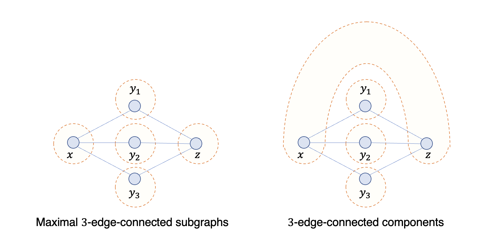
Figure 1: A graph $G$ where its maximal $3$-edge-connected subgraphs are different from its $3$-edge-connected components.

It is an intriguing question whether one can also obtain an almost-linear time algorithm for maximal $k$-edge-connected subgraphs, or there is a separation between these two closely related problems.

Our results.

In this paper, we show the first almost-linear time algorithm when $k=\log^{o(1)}n$, answering the above question affirmatively at least for small $k$.

Theorem 1.1.

There is a deterministic algorithm that, given an undirected unweighted graph $G$ with $n$ vertices and $m$ edges, computes the maximal $k$-edge-connected subgraphs of $G$ in $O(m+n^{1+o(1)})$ time for any $k=\log^{o(1)}n$.

Our techniques naturally extend to the decremental graph setting.

Theorem 1.2.

There is a deterministic algorithm that, given an undirected unweighted graph $G$ with $n$ vertices and $m$ edges undergoing a sequence of edge deletions, maintains the maximal $k$-edge-connected subgraphs of $G$ in $m^{1+o(1)}$ total update time for any $k=\log^{o(1)}n$.

Dynamic algorithms for maximal $k$-edge-connected subgraphs were recently studied in [GIKP22]. For comparison, their algorithm can handle both edge insertions and deletions but require $O(n\sqrt{n}\log n)$ worst-case update time, which is significantly slower than our $m^{o(1)}$ amortized update time. When $k=3$, they also gave an algorithm that handles edge insertions only using $\tilde{O}(n^{2})$ total update time.

Previous Approaches and Our Techniques.

Our approach diverges significantly from the local-cut-based approach in [CHI⁺17, FNS⁺20]. In these previous approaches, they call the local cut subroutine $\Omega(n)$ times and each call takes $\Omega(\sqrt{n})$ time. Hence, their running time is at least $\Omega(n\sqrt{n})$ and this seems inherent without significant modification. Recently, [GIKP22] took a different approach. Their $\tilde{O}(m+n^{3/2}k^{8})$-time algorithm efficiently implements the folklore recursive mincut algorithm by feeding $O(nk)$ updates to the dynamic minimum cut algorithm by Thorup [Tho07]. However, since Thorup’s algorithm has $\Omega(\sqrt{n})$ update time, the final running time of [GIKP22] is at least $\Omega(n\sqrt{n})$ as well.

Our algorithm is similar to [GIKP22] in spirit but is much more efficient. We instead apply the dynamic $k$-edge connectivity algorithms by Jin and Sun [JS22] that takes only $n^{o(1)}$ update time when $k=\log^{o(1)}n$. Our reduction is more complicated than the reduction in [GIKP22] to dynamic minimum cut because the data structure by [JS22] only supports pairwise $k$-edge connectivity queries, not a global minimum cut. Nonetheless, we show that $\tilde{O}(nk)$ updates and queries to this “weaker” data structure also suffice.

Our approach is quite generic. Our algorithm is carefully designed without the need to check if the graph for which the recursive call is made is $k$-edge-connected. This allows us to extend our algorithm to the dynamic case.

Organization.

We give preliminaries in Section 2. Then, we prove Theorem 1.1 and Theorem 1.2 in Section 3 and Section 4, respectively.

2 Preliminaries

Let $G=(V,E)$ be an unweighted undirected graph. Let $n=\left\lvert V\right\rvert$ and $m=\left\lvert E\right\rvert$, and assume $m=\mathrm{poly}(n)$ and $k=\log^{o(1)}n$. For any $S,T\subseteq V$, let $E(S,T)=\{(u,v)\in E\mid u\in S,v\in T\}$. For every vertex $u$, the degree of $u$ is $\deg(u)=\left\lvert\{(u,v)\mid(u,v)\in E\}\right\rvert$. For every subset of vertices $S\subseteq V$, the volume of $S$ is $\mathrm{vol}(S)=\sum_{u\in S}\deg(u)$. Denote $G[S]$ as the induced graph of $G$ on a subset of vertices $S\subseteq V$.

Two vertices $s$ and $t$ are $k$-edge-connected in $G$ if one needs to delete at least $k$ edges to disconnect $s$ and $t$ in $G$. A vertex set $S$ is $k$-edge-connected if every pair of vertices in $S$ is $k$-edge-connected. We use the convention that $S$ is $k$-edge-connected when $|S|=1$. We say that a graph $G=(V,E)$ is $k$-edge-connected if $V$ is $k$-edge-connected. A $k$-edge-connected component is an inclusion-maximal vertex set $S$ such that $S$ is $k$-edge-connected. A whole vertex set can always be partitioned into $k$-edge-connected components. We use $kECC(u)$ to denote the unique $k$-edge-connected component containing $u$. Note that a $k$-edge-connected component may not induce a connected graph when $k>2$. A vertex set $S$ is a $k$-cut if $|E(S,V\setminus S)|<k$. Note, however, we also count the whole vertex set $V$ as a trivial $k$-cut.

We will crucially exploit the following dynamic algorithm in our paper.

Theorem 2.1 (Dynamic pairwise $k$-edge connectivity [JS22]).

There is a deterministic algorithm that maintains a graph $G$ with $n$ vertices undergoing edge insertions and deletions using $n^{o(1)}$ update time and, given any vertex pair $(s,t)$, reports whether $s$ and $t$ are $k$-edge-connected in the current graph $G$ in $n^{o(1)}$ time where $k=\log^{o(1)}n$.

For the maximal $k$-edge-connected subgraph problem, we can assume that the graph is sparse using the forest decomposition.

Definition 2.2 (Forest decomposition [NI08]).

A $t$-forest decomposition of a graph $G$ is a collection of forests $F_{1},\ldots,F_{t}$, such that $F_{i}$ is a spanning forest of $G\setminus\bigcup_{j=1}^{i-1}F_{j}$, for every $1\leq i\leq t$.

Theorem 2.3 (Lemma 8.3 of [GIKP22]).

Any $O(k\log n)$-forest decomposition of a graph has the same maximal $k$-edge-connected subgraphs as the original graph. Moreover, there is an algorithm for constructing such a $O(k\log n)$-forest decomposition in $O(m)$ time.

3 The Static Algorithm

In this section, we prove our main result, Theorem 1.1. The key idea is the following reduction:

Lemma 3.1.

Suppose there is a deterministic decremental algorithm supporting pairwise $k$-edge-connectivity that has $t_{p}\cdot m$ total preprocessing and update time on an initial graph with $n$ vertices and $m$ edges and query time $t_{q}$.

Then, there is a deterministic algorithm for computing the maximal $k$-edge-connected subgraphs in $O(m+(t_{p}+t_{q})\cdot kn\log^{2}n)$ time.

By plugging in theorem 2.1, we get theorem 1.1. The rest of this section is for proving Lemma 3.1. Throughout this section, we let $t_{q}$ denote the query time of the decremental pairwise $k$-edge connectivity data structure that Lemma 3.1 assumes.

Recall again that, for any vertex $u$, $u$’s $k$-edge-connected component, $kECC(u)$, might not induce a connected graph. The first tool for proving Lemma 3.1 is a “local” algorithm for finding a connected component of $G[kECC(u)]$.

Lemma 3.2.

Given a graph $G$ and a vertex $u$, there is a deterministic algorithm for finding the connected component $U$ containing $u$ of $G[kECC(u)]$ in $O(t_{q}\cdot\mathrm{vol}(U))$ time.

Proof.

We run BFS from $u$ to explore every vertex in the connected component $U$ containing $u$ of $kECC(u)$. During the BFS process, we only visit the vertices in $kECC(u)$ by checking if the newly found vertex is $k$-edge-connected to $u$. Since each edge incident to $U$ is visited at most twice, the total running time is $O(t_{q}\cdot\mathrm{vol}(U))$. ∎

Below, we describe the algorithm for Lemma 3.1 in Algorithm 1 and then give the analysis.

Input: An undirected connected graph $G=(V,E)$, and a list of vertices $L$ (initially $L=V$). Note that the parameters are passed by value.

Output: The maximal $k$-edge-connected subgraphs of $G$.

1

2$S\leftarrow\varnothing$.

3 while $\left\lvert L\right\rvert>1$ do

4       Choose an arbitrary pair $(u,v)\in L$.

5       if $u$ and $v$ are $k$-edge-connected in $G$ then

6             $L\leftarrow L\setminus\{v\}$.

7            

8      else

9             Simultaneously compute the $u$’s connected component of $G[kECC(u)]$ and the $v$’s connected component of $G[kECC(v)]$, until the one with the smaller volume (denoted by $U$) is found.

10             $S\leftarrow S\cup\textsc{Main}(G[U],U)$.

11             $G\leftarrow G\setminus U$.

12             $L\leftarrow(L\setminus U)\cup\{w\notin U\mid(x,w)\in E(U,V(G)\setminus U)\}$.

13       end if

14      

15 end while

16$S\leftarrow S\cup\{V(G)\}$.

17 return $S$.

Algorithm 1 $\textsc{Main}(G,L)$: compute the maximal $k$-edge-connected subgraphs

Correctness.

We start with the following structural lemma.

Lemma 3.3 (Lemma 5.6 of [CHI⁺17]).

Let $T$ be a $k$-cut in $G[C]$ for some vertex set $C$. Then, either

• $T$ is a $k$-cut in $G$ as well, or

• $T$ contains an endpoint of $E(C,V(G)\setminus C)$.

Next, the crucial observation of our algorithm is captured by the following invariant.

Lemma 3.4.

At any step of Algorithm 1, every $k$-cut $T$ in $G$ is such that $T\cap L\neq\emptyset$.

Proof.

The base case is trivial because $L\leftarrow V$ initially. Next, we prove the inductive step. $L$ can change in Line 1 or Line 1.

In the first case, the algorithm finds that $u$ and $v$ are $k$-edge-connected and removes $v$ from $L$. For any $k$-cut $T$ where $v\in T$, an important observation is that $kECC(v)\subseteq T$ as well. But $kECC(u)=kECC(v)$ and so $u\in T$ too. So the invariant still holds even after removing $v$ from $L$.

In the second case, the algorithm removes $U$ from $G$. Let us denote $G^{\prime}=G\setminus U$. Since the algorithm adds the endpoints of cut edges crossing $U$ to $L$, it suffices to consider a $k$-cut $T$ in $G^{\prime}$ that is disjoint from the endpoints of the cut edges of $U$. By Lemma 3.3, $T$ was a $k$-cut in $G$. Since the changes in $L$ occur only at $U$ and neighbors of $U$, while $T$ is disjoint from both $U$ and all neighbors of $U$, we have $T\cap L\neq\emptyset$ by the induction hypothesis. ∎

Corollary 3.5.

When $|L|=1$, then $G$ is $k$-edge-connected.

Proof.

Otherwise, there is a partition $(A,B)$ of $V$ where $|E(A,B)|<k$. So both $A$ and $B$ are $k$-cuts in $G$. By Lemma 3.4, $A\cap L\neq\emptyset$ and $B\cap L\neq\emptyset$ which contradicts that $|L|=1$. ∎

We are ready to conclude the correctness of Algorithm 1. At a high level, the algorithm finds the set $U$ and “cuts along” $U$ at Lines 1. Then, on one hand, recurse on $U$ at Line 1 and, on the other hand, continue on $V(G)\setminus U$. We say that the cut edges $E(U,V(G)\setminus U)$ are “deleted”.

Now, since $U$ is the connected component of $G[kECC(u)]$ for some vertex $u$. We have that, for every edge $(x,y)\in E(U,V(G)\setminus U)$, the pair $x$ and $y$ are not $k$-edge-connected in $G$. In particular, $x$ and $y$ are not $k$-edge-connected in $G[V^{\prime}]$ for every $V^{\prime}\subseteq V$.

Thus, the algorithm never deletes edges inside any maximal $k$-edge-connected subgraph $V_{i}$. Since the algorithm stops only when the remaining graph is $k$-edge-connected, the algorithm indeed returns the maximal $k$-edge-connected subgraphs of the whole graph.

Running Time.

Consider the time spent on each recursive call. Let $G^{\prime}$ be the graph for which the recursive call is made and $m^{\prime}=\mathrm{vol}(G^{\prime})$. Every vertex is inserted to $L$ initially or as an endpoint of some removed edge, so the total number of vertices added to $L$ is $O(m^{\prime})$. In each iteration, either we remove a vertex from $L$, or remove a subgraph from $G$. Hence we check pairwise $k$-edge-connectivity $O(m^{\prime})$ times, so the running time of checking pairwise $k$-edge-connectivity is $O(t_{q}\cdot m^{\prime})$. For the time of finding connected components of $k$-edge-connected components, since we spend $O(t_{q}\cdot\mathrm{vol}(U))$ time to find some $U$ and remove $U$ from $G$, the total cost is $O(t_{q}\cdot m^{\prime})$. Plus, initializing the dynamic pairwise $k$-edge connectivity algorithm on $G^{\prime}$ takes $O(t_{p}\cdot m^{\prime})$ time. Thus the total running time of each recursive call is $O((t_{p}+t_{q})\cdot m^{\prime})$.

For the recursion depth, since each $U$ found has the smaller volume of the two, $\mathrm{vol}(U)\leq m^{\prime}/2$. Hence the recursion depth is $O(\log m_{0})$, where $n_{0}$ and $m_{0}$ are the numbers of vertices and edges of the initial graph. Thus the total running time of Algorithm 1 is $O((t_{p}+t_{q})\cdot m_{0}\log n_{0})$.

By applying theorem 2.3 to the initial graph $G$ and invoking Algorithm 1 on the resulting graph, the number of edges in the resulting graph is $O(kn_{0}\log n_{0})$, so the running time is improved to $O(m_{0}+(t_{p}+t_{q})\cdot kn_{0}\log^{2}n_{0})$. This completes the proof of Lemma 3.1.

4 The Decremental Algorithm

Our static algorithm can be naturally extended to a decremental dynamic algorithm. To prove Theorem 1.2, we prove the following reduction. By combining Lemma 4.1 and Theorem 2.1, we are done.

Lemma 4.1.

Suppose there is a deterministic decremental algorithm supporting pairwise $k$-edge-connectivity that has $t_{p}\cdot m$ total preprocessing and update time on an initial graph with $n$ vertices and $m$ edges and query time $t_{q}$.

Then there is a deterministic decremental dynamic algorithm for maintaining the maximal $k$-edge-connected subgraphs on an undirected graph of $n$ vertices and $m$ edges with $O((t_{p}+t_{q})\cdot m\log n)$ total preprocessing and update time, and $O(1)$ query time.

The algorithm for Lemma 4.1 as is follows. First, we preprocess the initial graph $G_{0}$ using Algorithm 1 and obtain the maximal $k$-edge-connected subgraphs $\{V_{1},\dots,V_{z}\}$ of $G_{0}$.

Next, given an edge $e$ to be deleted, if $e$ is in a maximal $k$-edge-connected subgraph $V_{i}$ of $G$, then we invoke $\textsc{Update}(G[V_{i}],e)$ and update the set of the maximal $k$-edge-connected subgraphs of $G$; otherwise we ignore $e$. The subroutine $\textsc{Update}(H,e)$ is described in Algorithm 2.

Input: A $k$-edge-connected subgraph $H$ and an edge $e=(x,y)\in H$ to be deleted.

Output: The $k$-edge-connected subgraphs of $H$ after deletion.

1 $H\leftarrow H\setminus\{(x,y)\}$.

2 return $\textsc{Main}(H,\{x,y\})$.

3

Algorithm 2 Update(H, e)

Correctness.

Let $H=(V^{\prime},E^{\prime})$ be the maximal $k$-edge-connected subgraph containing edge $(x,y)$ before deletion. It suffices to prove that Lemma 3.4 holds when we invoke Algorithm 1. Suppose there is a $k$-cut $C$ in $H\setminus\{(x,y)\}$ such that $C\cap\{x,y\}=\emptyset$, then $C$ is also a $k$-cut in $H$, a contradiction. Hence the correctness follows from the correctness of Algorithm 1.

Running Time.

In the case that $H\setminus\{(x,y)\}$ is still $k$-edge-connected, the running time is $t_{q}$. We charge this time $t_{q}$ to the deleted edge $(x,y)$.

Otherwise, consider the time spend on each recursive call of Main. Assume that the total volume of the subgraphs removed and passed to another recursive call in a recursive call is $\nu$. The total number of vertices added to $L$ is $O(\nu)$. In each iteration, we either remove a vertex from $L$ or remove a subgraph. Hence we check pairwise $k$-edge-connectivity $O(\nu)$ times, so the running time of checking pairwise $k$-edge-connectivity is $O(t_{q}\cdot\nu)$. Since we spend $O(t_{q}\cdot\mathrm{vol}(U))$ time to find $U$, the total cost is $O(t_{q}\cdot\nu)$. Plus, it takes $O((t_{p}+t_{q})\cdot m^{\prime})$ time to initialize the dynamic pairwise $k$-edge connectivity algorithm and check pairwise $k$-edge-connectivity on a graph $H^{\prime}$ with $m^{\prime}$ edges for the first time we invoke Main on $H^{\prime}$. Also, removing all edges from $H^{\prime}$ takes $t_{p}\cdot m^{\prime}$ time. We charge $O(t_{p}+t_{q})$ to each of the removed edges in each recursive call.

The recursion depth is $O(\log m_{0})$ by Lemma 3.1, where $n_{0}$ and $m_{0}$ are the numbers of vertices and edges of the initial graph. Hence each edge will be charged $O(\log m_{0})$ times, so the total preprocessing and update time is $O((t_{p}+t_{q})\cdot m_{0}\log n_{0})$.

Appendix A Relationship with $k$-Edge-Connected Components

The reason why a subroutine for computing $k$-edge-connected components is not useful for computing maximal $k$-edge-connected subgraphs is as follows. Given a graph $G=(V,E)$, we can artificially create a supergraph $G^{\prime}=(V^{\prime}\supseteq V,E^{\prime}\supseteq E)$ where the whole set $V$ is $k$-edge-connected, but the maximal $k$-edge-connected subgraphs of $G^{\prime}$ will reveal the maximal $k$-edge-connected subgraphs of $G$. So given a subroutine for computing the $k$-edge-connected components of $G^{\prime}$, we know nothing about the maximal $k$-edge-connected subgraphs of $G$. The construction of $G^{\prime}$ is as follows.

First, we set $G^{\prime}\leftarrow G$. Assume $V=\{1,2,\ldots,n\}$. For every $1\leq i<n$, add $k$ parallel dummy length-$2$ paths $(i,d_{i,1},i+1),\ldots,(i,d_{i,k},i+1)$. Thus $i$ and $i+1$ are $k$-edge-connected, so $V$ is $k$-edge-connected at the end. When we compute the maximal $k$-edge-connected subgraphs of $G^{\prime}$, we know that we will first remove all dummy vertices $d_{i,j}$ because they all have degree $2$ (assuming that $k>2$). We will obtain $G$ and so we will obtain the maximal $k$-edge-connected subgraphs of $G$ from this process.

References

- [AIY13] Takuya Akiba, Yoichi Iwata, and Yuichi Yoshida. Linear-time enumeration of maximal k-edge-connected subgraphs in large networks by random contraction. In Proceedings of the 22nd ACM international conference on Information & Knowledge Management, pages 909–918, 2013.
- [AKL+22] Amir Abboud, Robert Krauthgamer, Jason Li, Debmalya Panigrahi, Thatchaphol Saranurak, and Ohad Trabelsi. Breaking the cubic barrier for all-pairs max-flow: Gomory-hu tree in nearly quadratic time. In 2022 IEEE 63rd Annual Symposium on Foundations of Computer Science (FOCS), pages 884–895. IEEE, 2022.
- [CHI+17] Shiri Chechik, Thomas Dueholm Hansen, Giuseppe F Italiano, Veronika Loitzenbauer, and Nikos Parotsidis. Faster algorithms for computing maximal 2-connected subgraphs in sparse directed graphs. In Proceedings of the Twenty-Eighth Annual ACM-SIAM Symposium on Discrete Algorithms, pages 1900–1918. SIAM, 2017.
- [FNS+20] Sebastian Forster, Danupon Nanongkai, Thatchaphol Saranurak, Liu Yang, and Sorrachai Yingchareonthawornchai. Computing and testing small connectivity in near-linear time and queries via fast local cut algorithms. In Proceedings of the Fourteenth Annual ACM-SIAM Symposium on Discrete Algorithms, pages 2046–2065. SIAM, 2020.
- [GIKP22] Loukas Georgiadis, Giuseppe F Italiano, Evangelos Kosinas, and Debasish Pattanayak. On maximal 3-edge-connected subgraphs of undirected graphs. arXiv preprint arXiv:2211.06521, 2022.
- [HRG00] Monika R Henzinger, Satish Rao, and Harold N Gabow. Computing vertex connectivity: new bounds from old techniques. Journal of Algorithms, 34(2):222–250, 2000.
- [JS22] Wenyu Jin and Xiaorui Sun. Fully dynamic st edge connectivity in subpolynomial time. In 2021 IEEE 62nd Annual Symposium on Foundations of Computer Science (FOCS), pages 861–872. IEEE, 2022.
- [Kar00] David R Karger. Minimum cuts in near-linear time. Journal of the ACM (JACM), 47(1):46–76, 2000.
- [NI08] Hiroshi Nagamochi and Toshihide Ibaraki. Algorithmic Aspects of Graph Connectivity. Encyclopedia of Mathematics and its Applications. Cambridge University Press, 2008.
- [NS23] Chaitanya Nalam and Thatchaphol Saranurak. Maximal k-edge-connected subgraphs in weighted graphs via local random contraction. In Proceedings of the 2023 Annual ACM-SIAM Symposium on Discrete Algorithms (SODA), pages 183–211. SIAM, 2023.
- [SHB+16] Heli Sun, Jianbin Huang, Yang Bai, Zhongmeng Zhao, Xiaolin Jia, Fang He, and Yang Li. Efficient k-edge connected component detection through an early merging and splitting strategy. Knowledge-Based Systems, 111:63–72, 2016.
- [Tar72] Robert Tarjan. Depth-first search and linear graph algorithms. SIAM journal on computing, 1(2):146–160, 1972.
- [Tho07] Mikkel Thorup. Fully-dynamic min-cut. Combinatorica, 27(1):91–127, 2007.
- [YQL+16] Long Yuan, Lu Qin, Xuemin Lin, Lijun Chang, and Wenjie Zhang. I/o efficient ecc graph decomposition via graph reduction. Proceedings of the VLDB Endowment, 2016.
- [YZH05] Xifeng Yan, X Jasmine Zhou, and Jiawei Han. Mining closed relational graphs with connectivity constraints. In Proceedings of the eleventh ACM SIGKDD international conference on Knowledge discovery in data mining, pages 324–333, 2005.
- [ZLY+12] Rui Zhou, Chengfei Liu, Jeffrey Xu Yu, Weifa Liang, Baichen Chen, and Jianxin Li. Finding maximal k-edge-connected subgraphs from a large graph. In Proceedings of the 15th international conference on extending database technology, pages 480–491, 2012.