Large-scale Bayesian Structure Learning for Gaussian Graphical Models using Marginal Pseudo-likelihood

Abstract

Bayesian methods for learning Gaussian graphical models offer a robust framework that addresses model uncertainty and incorporates prior knowledge. Despite their theoretical strengths, the applicability of Bayesian methods is often constrained by computational needs, especially in modern contexts involving thousands of variables. To overcome this issue, we introduce two novel Markov chain Monte Carlo (MCMC) search algorithms that have a significantly lower computational cost than leading Bayesian approaches. Our proposed MCMC-based search algorithms use the marginal pseudo-likelihood approach to bypass the complexities of computing intractable normalizing constants and iterative precision matrix sampling. These algorithms can deliver reliable results in mere minutes on standard computers, even for large-scale problems with one thousand variables. Furthermore, our proposed method is capable of addressing model uncertainty by efficiently exploring the full posterior graph space. Our simulation study indicates that the proposed algorithms, particularly for large-scale sparse graphs, outperform the leading Bayesian approaches in terms of computational efficiency and precision. The implementation supporting the new approach is available through the R package BDgraph.

Keywords: Markov random field; Model selection; Link prediction; Network reconstruction; Bayes factor.

1 Introduction

In statistical modeling, graphical models (Lauritzen, 1996; Koller and Friedman, 2009) stand out as a principal tool for assessing conditional dependencies among variables. Conditional dependence denotes the relationship between two or more variables with the effect of other variables removed. These conditional dependencies are elegantly portrayed using graphs, where nodes represent random variables (Lauritzen, 1996). Within the context of undirected graphs, the absence of an edge between two nodes implies conditional independence between the variables they represent (Rue and Held, 2005). Estimating that underlying graph structure is called structure learning.

In this article, we consider Bayesian structure learning approaches for estimating Gaussian graphical models (GGMs), in contrast with frequentist techniques like the lasso-based neighborhood selection that commonly optimize the likelihood function (Friedman et al., 2008; Peng et al., 2009; Meinshausen and Bühlmann, 2006). The strength of Bayesian approaches lies in handling model uncertainty through posterior distributions and accommodating prior knowledge. Yet, with increasing dimensions, Bayesian methods often lag in computational speed and scalability relative to frequentist alternatives.

The primary objective of Bayesian structure learning methods is to determine the underlying graph structure given the data (Vogels et al., 2023). Bayesian paradigms can achieve this by computing the posterior distribution of the graph conditional on the data. For the case of GGMs, this requires the calculation of a complex integral, a task that becomes increasingly challenging, or even impractical, for larger-scale graphs. Thus, most Bayesian methods (Mohammadi et al., 2023; van den Boom et al., 2022; Peterson et al., 2015; Niu et al., 2023) compute the joint posterior distribution of the graph and precision matrix.

A comprehensive exploration of this joint posterior distribution is feasible only for very small graphs (with 10 nodes or less). This limitation arises because the possible number of graphical models escalates at a super-exponential rate with the number of nodes. Therefore, most Bayesian methods deploy sampling algorithms over the joint space of graphs and precision matrices, primarily using Markov chain Monte Carlo (MCMC) sampling. Green (1995) proposed the so-called reversible jump MCMC, which is based on a discrete-time Markov chain. Dobra et al. (2011) implemented the reversible jump MCMC sampling of Green (1995) for GGMs. The derivation of joint posterior distribution requires the prior distribution of the precision matrix given the graph. Most Bayesian methods for Gaussian likelihood, use a $G$-Wishart distribution (Roverato, 2002; Letac and Massam, 2007) as a natural conjugate prior for the precision matrix. A computationally expensive step within the search algorithm is to determine the ratio of prior normalizing constants for the $G$-Wishart distribution (Mohammadi et al., 2023). Advancements in reducing calculation time have been suggested by Wang and Li (2012), Cheng and Lenkoski (2012), and Mohammadi et al. (2023). Moreover, Lenkoski (2013), Hinne et al. (2014), and van den Boom et al. (2022) proposed computationally efficient algorithms to sample from the $G$-Wishart distribution. Further efficiency was achieved by Mohammadi and Wit (2015), who proposed a search algorithm known as the birth-death MCMC algorithm, which is based on a continuous-time Markov chain, to explore the graph space more efficiently. As an alternative to methods reliant on the $G$-Wishart prior, Wang (2015) introduced a block Gibbs algorithm using a spike-and-slab prior distribution. This approach allows for updating the entire columns of the precision matrix at once, leading to faster convergence of the MCMC algorithm.

The computational challenge of the existing MCMC-based search algorithms is that they evaluate the joint posterior distribution of the graph and precision matrix rather than the posterior distribution of the graph alone. During each MCMC iteration, these algorithms encounter two computational issues: (i) the difficult-to-compute normalizing constants that require approximation, and (ii) the update of the precision matrix. Existing MCMC-based methods are therefore computationally expensive from 100 variables upward for the reversible jump and birth-death MCMC algorithms, and from 250 variables upward for the spike-and-slab approach introduced by Wang (2015). These computational costs restrict the applicability of Bayesian methods in modern applications that involve thousands of variables.

The main contribution of this article is to introduce a novel MCMC-based methodology for GGMs. Instead of focusing on the joint posterior distribution of the graph and precision matrix, we work with the posterior distribution of the graph. In this way, we bypass the challenges associated with constant normalization and repeated precision matrix sampling. In our approach, rather than using the Gaussian likelihood function that requires the precision matrix to be positive definite, we replace it with pseudo-likelihood that is a product of conditional likelihood functions (Besag, 1975). We introduce two MCMC-based search algorithms that leverage the marginal pseudo-likelihood (MPL) approach for enhanced computational efficiency. The MPL approach has been adapted in graphical models (Ji and Seymour, 1996; Ravikumar et al., 2010; Niu et al., 2023). Previous studies, such as those by Pensar et al. (2017) as well as Dobra and Mohammadi (2018) have applied MPL to undirected graphical models with discrete variables. The similar MPL approaches were implemented by Consonni and Rocca (2012) and Carvalho and Scott (2009) in GGMs but limited to decomposable graphs. Leppä-Aho et al. (2017) used this approach for non-decomposable graphs by implementing a score based hill-climbing algorithm. This approach is constrained to the maximum a posterior probability approach, by estimating the posterior mode and not the full posterior.

To demonstrate the computational efficiency and graph recovery precision of our proposed MCMC-based search algorithms, we point to Figure 1. This figure shows the area under the ROC curve (AUC) of several methods as a function of computation time for a cluster graph structure with $1000$ nodes and $10000$ samples. This visualization is part of our extensive simulation study in Section 4. An evident takeaway is the much faster convergence behavior of our proposed MCMC-based algorithms (BD-MPL and RJ-MPL) than the leading Bayesian methods, such as the SS method (Wang, 2015) and the BD method (Mohammadi and Wit, 2015; Mohammadi et al., 2023). The plot indicates that the BD-MPL algorithm quickly reaches impressive AUC values (exceeding 0.98) in roughly two minutes (126 seconds). In contrast, the SS algorithm requires an entire day to reach a decent AUC, and even fails to meet a comparable AUC level even after five days. The BD algorithm struggles with such large-scale graphs and remains near an AUC of roughly $0.5$ after four days.

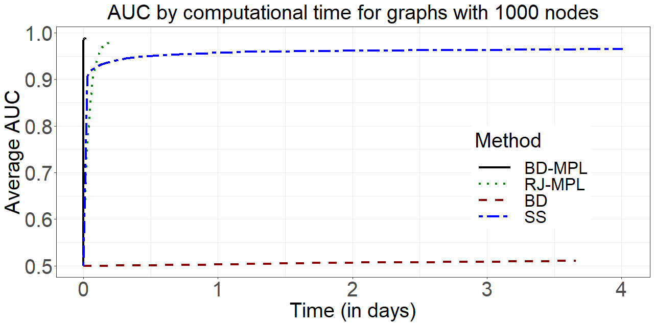
Figure 1: AUC as a function of computational time for the cluster graph with $1000$ nodes and $10000$ observations. The BD-MPL and RJ-MPL refer to our proposed MCMC-based search algorithms (Algorithms 1 and 2, respectively). The SS stands for a leading Bayesian method presented by Wang (2015), while BD represents the birth-death MCMC search algorithm developed by Mohammadi and Wit (2015) and Mohammadi et al. (2023). The plot shows the average AUC value over 10 replications. This plot is part of the simulation study in Section 4.

The article is organized as follows. Section 2 delves into the fundamental concepts of Bayesian structure learning for GGMs. Section 3 details the marginal pseudo-likelihood approach along with the two proposed MCMC-based search algorithms. In Section 4, we assess the efficacy of these new algorithms, in comparison to current leading Bayesian methods. We conclude with reflections and potential avenues for future exploration. Our implementation is included in the R package BDgraph at http://cran.r-project.org/packages=BDgraph.

2 Bayesian Structure Learning for GGMs

We denote an undirected graph by $G=(V,E)$, where $V$ contains $p$ nodes corresponding to the $p$ coordinates and the set of edges is denoted by $E\subset\{(i,j)|1\leq i<j\leq p\}$. In this notation, the edge $(i,j)$ denotes the link between nodes $i$ and $j$. Here, each node represents a distinct random variable. All nodes together form a $p$-dimensional random vector. We have a data matrix $\boldsymbol{X}=(\boldsymbol{X}^{(1)},\ldots,\boldsymbol{X}^{(n)})^{T}$ of dimensions $n\times p$. The independent samples/rows, $\boldsymbol{X}^{(k)}$ for $k\in\{1,\ldots,n\}$, correspond to $p$-dimensional random vectors. In Gaussian graphical models, each $\boldsymbol{X}^{(k)}$ is distributed according to a multivariate Gaussian distribution $\mathcal{N}_{p}(\boldsymbol{0},\boldsymbol{\Sigma})$ with $\boldsymbol{\Sigma}$ being the covariance matrix. The corresponding precision matrix is denoted by $\boldsymbol{K}=\boldsymbol{\Sigma}^{-1}$ with elements $K_{ij}$. Notes $i$ and $j$ are conditionally independent if and only if $K_{ij}=0$ (Lauritzen, 1996).

In Bayesian structure learning, the ultimate aim is to estimate the posterior probability of the graph $G$ conditional on the data $\boldsymbol{X}$:

$$P(G|\boldsymbol{X})\propto P(\boldsymbol{X}|G)P(G),$$ (1)

where $P(G)$ is the prior of a graph $G$ and $P(\boldsymbol{X}|G)$ is the marginal likelihood of $G$.

For the prior distribution of the graph, one can assign constant probabilities denoted by $\beta_{ij}\in(0,1)$, for including each edge $e=(i,j)$ in $G$. If all $\beta_{ij}$ values are set equal to $\beta\in(0,1)$, it leads to the following prior distribution

$$P(G)\propto\beta^{|E|}(1-\beta)^{|\bar{E}|},$$ (2)

where $\bar{E}$ denotes to the set of edges that are not in $G$. For sparser graphs, a lower value of $\beta$ is recommended. When $\beta=0.5$, the prior becomes non-informative and uniformly distributed over the graph space. We should mention that our Bayesian framework is not limited to this prior and can accommodate any prior distribution on $G$. For other choices of priors for graph $G$, we refer to Dobra et al. (2011); Jones et al. (2005); Mohammadi and Wit (2015); Scutari (2013).

For the marginal likelihood of $G$, we have

$$P(\boldsymbol{X}|G)=\int_{\boldsymbol{K}}P(\boldsymbol{X}|G,\boldsymbol{K})P(\boldsymbol{K}|G)d\boldsymbol{K},$$ (3)

where $P(\boldsymbol{K}|G)$ denotes the prior for $\boldsymbol{K}$ given $G$ and $P(\boldsymbol{X}|G,\boldsymbol{K})$ is the likelihood function.

A popular and well known choice for the prior distribution of the precision matrix $\boldsymbol{K}$ is the $G$-Wishart distribution (Roverato, 2002; Letac and Massam, 2007) and it is the conjugate prior for $P(\boldsymbol{K}|G)$. The $G$-Wishart density is

$$P(\boldsymbol{K}|G)=\frac{1}{I_{G}(b,\boldsymbol{D})}|\boldsymbol{K}|^{\frac{b-2}{2}}\exp\{\frac{-1}{2}\mbox{tr}(\boldsymbol{K}\boldsymbol{D})\}\mathbf{1}_{P_{G}}(\boldsymbol{K}),$$

where $|\boldsymbol{K}|$ denotes the determinant of $\boldsymbol{K}$, $tr(\boldsymbol{A})$ is the trace of a square matrix $\boldsymbol{A}$, $P_{G}$ is the set of positive definite matrices $\boldsymbol{K}$ with $K_{ij}=0$ if $(i,j)\notin E$, and $\mathbf{1}_{P_{G}}(\boldsymbol{K})$ is an indicator function that equals 1 if $\boldsymbol{K}\in P_{G}$ and 0 otherwise. The symmetric positive definite matrix $\boldsymbol{D}$ and the scalar $b>2$ are the scale and the shape parameters of the $G$-Wishart distribution, respectively. Here, $I_{G}(b,\boldsymbol{D})$ is the normalizing constant, which is given by

$$I_{G}(b,\boldsymbol{D})=\int_{\boldsymbol{K}\in P_{G}}|\boldsymbol{K}|^{\frac{b-2}{2}}\exp\{\frac{-1}{2}\mbox{tr}(\boldsymbol{K}\boldsymbol{D})\}d\boldsymbol{K}.$$

Using the $G$-Wishart prior, Equation (3) becomes

$$P(\boldsymbol{X}|G)=(2\pi)^{-\frac{np}{2}}\frac{I_{G}(b+n,\boldsymbol{D}+\boldsymbol{U})}{I_{G}(b,\boldsymbol{D})},$$

where $\boldsymbol{U}=\boldsymbol{X}^{T}\boldsymbol{X}$. This ratio of normalizing constants is hard to calculate (Atay-Kayis and Massam, 2005; Mohammadi et al., 2023; Uhler et al., 2018). Therefore most Bayesian structure learning methods approximate it by utilizing MCMC sample algorithms over the joint space of graphs and precision matrices.

The joint posterior distribution of the graph $G$ and the precision matrix $\boldsymbol{K}$ is given by

$$\begin{split}P(G,\boldsymbol{K}|\boldsymbol{X})&\propto P(\boldsymbol{X}|\boldsymbol{K},G)P(\boldsymbol{K}|G)P(G)\\ &\propto P(G)\frac{1}{I_{G}(b,\boldsymbol{D})}|\boldsymbol{K}|^{\frac{b+n-2}{2}}\exp\{\frac{-1}{2}\mbox{tr}(\boldsymbol{K}(\boldsymbol{D}+\boldsymbol{U}))\}.\end{split}$$ (4)

Computing the above joint posterior distribution becomes computationally infeasible for $p>10$ due to the exponential growth of the number of potential graphs. To estimate $P(G,\boldsymbol{K}|\boldsymbol{X})$, most Bayesian structure learning methods therefore use MCMC-based search algorithms. A well-known sampling algorithm for GGMs is the reversible jump MCMC algorithm (Green, 1995) based on a discrete-time Markov chain, which was used for Gaussian graphical models by Dobra et al. (2011); Lenkoski and Dobra (2011); Cheng and Lenkoski (2012); Lenkoski (2013); Hinne et al. (2014). During each MCMC iteration $s\in\{1,\ldots,S\}$, the state of the Markov chain is denoted by $(G^{(s)},\boldsymbol{K}^{(s)})$ and the chain jumps to state $(G^{(s+1)},\boldsymbol{K}^{(s+1)})$. For a sufficiently large number of iterations, $S$, the distribution of the sample pairs $\{(G^{(1)},\boldsymbol{K}^{(1)}),\ldots,(G^{(S)},\boldsymbol{K}^{(S)})\}$ approximates the posterior distribution $P(G,\boldsymbol{K}|\boldsymbol{X})$. The reversible jump MCMC algorithm explores the graph space by adding or removing one edge per iteration. In each iteration a new graph $G^{\prime}$ is proposed by adding or removing an edge from the current graph $G$. A transition to the proposed graph $G^{\prime}$ is subsequently accepted with a probability given by

$$\alpha(G,G^{\prime})=\min\left\{\frac{P(G^{\prime},\boldsymbol{K}^{\prime}|\boldsymbol{X})}{P(G,\boldsymbol{K}|\boldsymbol{X})},1\right\}.$$

This requires computing the ratio of posterior probabilities which can be considered as the conditional Bayes factor for two adjacent graphs. The primary computational challenge for many search algorithms is determining this ratio. To compute this ratio, the following computationally expensive ratio of normalizing constants needs to be determined

$$\frac{I_{G^{(s+1)}}(b,\boldsymbol{D})}{I_{G^{(s)}}(b,\boldsymbol{D})}.$$ (5)

Given the new graph $G^{(s+1)}$, a new precision matrix $\boldsymbol{K}^{(s+1)}$ needs to be derived by sampling from the $G^{(s+1)}$-Wishart distribution. This step is also computationally expensive. Following the introduction of the reversible jump MCMC for Bayesain structure learning, numerous enhancements have been suggested to minimize its high computational demand. Approximations for the ratio of normalizing constants (5) were presented by Wang (2012), Cheng and Lenkoski (2012), and Mohammadi et al. (2023). Lenkoski (2013) proposed an effective sampling technique designed to reduce the time needed to sample from the $G$-Wishart distribution. Hinne et al. (2014) leveraged techniques rooted in conditional Bayes factors to cut down on computational time. More recently, van den Boom et al. (2022) introduced the $G$-Wishart weighted proposal method to improve MCMC mixing and reduce computational cost.

The reversible jump algorithms often suffer from low acceptance rates, requiring more MCMC iterations to converge. To overcome this issue, Mohammadi and Wit (2015) proposed an alternative MCMC-based search algorithm rooted in a continuous-time Markov chain process. This search algorithm explores the graph space by jumping to neighboring graphs. Each jump removes or adds an edge. The jumps are birth-death events that are modeled as independent Poisson processes. Consequently, the time between successive events follows an exponential distribution. In every state $(G^{(s)},\boldsymbol{K}^{(s)})$, the chain spends a waiting time in that state before it jumps to a new state $(G^{(s+1)},\boldsymbol{K}^{(s+1)})$. Once a substantial number of jumps have been made, the samples $(G^{(s)},\boldsymbol{K}^{(s)})$, weighted by their respective waiting times, serve as an approximation to the posterior distribution $P(G,\boldsymbol{K}|\boldsymbol{X})$.

Despite the above improvements, reversible jump and birth-death search algorithms demand significant computational time. This is largely due to the necessity to sample a precision matrix from the G-Wishart distribution at each iteration and the fact that the graph changes by at most one edge during each iteration. To address these challenges, Wang (2015) proposed a block Gibbs sampler by considering the spike-and-slab prior. This prior facilitates the development of an MCMC algorithm capable of updating entire columns of $\boldsymbol{K}$ in each iteration. Despite these improvements, these algorithms still face computational challenges with large-scale graphs. This is primarily due to the continual need to sample from the precision matrix in every iteration, as pointed out by Vogels et al. (2023) as well as in our simulation study in Section 4.

3 Bayesian Structure Learning with Marginal Pseudo-Likelihood

We introduce two novel MCMC-based search algorithms by using the marginal pseudo-likelihood (MPL) approach. This is explored in conjunction with birth-death and reversible jump MCMC algorithms. In Section 3.1, we illustrate how the MPL approach facilitates the derivation of Bayes factors for MCMC search algorithms. The birth-death and reversible jump MCMC-based search algorithms are detailed in Sections 3.2 and 3.3, respectively.

Recall that we aim to reduce computational cost by computing $P(G|\boldsymbol{X})$ from Equation (1) instead of $P(G,\boldsymbol{K}|\boldsymbol{X})$ from Equation (4). In other words, we aim to sample over the graph space instead of the joint space of graphs and precision matrices. Direct computation of the posterior probability $P(G|\boldsymbol{X})$ for all potential graphs $G$ is feasible just for graphs with less than 10 nodes. This is due to the enormous size of the graph space. We therefore use MCMC-based search algorithms.

3.1 Marginal Pseudo-Likelihood

Bayesian structure learning for GGMs requires to design computationally efficient search algorithms, as we show in Sections 3.2 and 3.3. These type of search algorithms need to compute the Bayes factors of two neighboring graphs

$$\frac{P(G^{\prime}|\boldsymbol{X})}{P(G|\boldsymbol{X})}=\frac{P(G^{\prime})P(\boldsymbol{X}|G^{\prime})}{P(G)P(\boldsymbol{X}|G)},$$ (6)

where graphs $G=(V,E)$ and $G^{\prime}$ differ by a single edge $e=(i,j)$, that is $G^{\prime}=(V,E\cup e)$ or $G^{\prime}=(V,E\backslash e)$. To compute $P(G|\boldsymbol{X})$, we need to calculate the marginal likelihood $P(\boldsymbol{X}|G)$ in Equation (3), which does not have a closed form expression. Thus, we calculate $P(\boldsymbol{X}|G)$ by utilizing the MPL approach

$$P(\boldsymbol{X}|G)\approx\prod_{h=1}^{p}P(\boldsymbol{X}_{h}|\boldsymbol{X}_{nb(h)},G),$$ (7)

where $nb(h)$ refers to the neighbors of node $h$ and $\boldsymbol{X}_{nb(h)}$ is the sub-matrix obtained by selecting the columns in $\boldsymbol{X}$ corresponding to the nodes/variables that are in $nb(h)$. We then have

$$\begin{split}\frac{P(\boldsymbol{X}|G^{\prime})}{P(\boldsymbol{X}|G)}&\approx\frac{\prod_{h=1}^{p}P(\boldsymbol{X}_{h}|\boldsymbol{X}_{nb(h)},G^{\prime})}{\prod_{h=1}^{p}P(\boldsymbol{X}_{h}|\boldsymbol{X}_{nb(h)},G)}\\ &=\frac{P(\boldsymbol{X}_{i}|\boldsymbol{X}_{nb(i)},G^{\prime})P(\boldsymbol{X}_{j}|\boldsymbol{X}_{nb(j)},G^{\prime})}{P(\boldsymbol{X}_{i}|\boldsymbol{X}_{nb(i)},G)P(\boldsymbol{X}_{j}|\boldsymbol{X}_{nb(j)},G)}.\end{split}$$ (8)

For the last step, we use the fact that the graphs $G$ and $G^{\prime}$ are the same except that one edge $e=(i,j)$ is added or removed while moving from $G$ to $G^{\prime}$. As a result, the probabilities of all nodes except $X_{i}$ and $X_{j}$ are the same and can be removed from the fraction.

The fractional pseudo-likelihoods in Equation (8) can be expressed in a closed-form by considering a non-informative fractional prior on $\boldsymbol{K}$ as $W_{p}(p,\boldsymbol{U}/n)$, where $W_{p}(a,\boldsymbol{A})$ represents a Wishart distribution with an expected value of $a\boldsymbol{A}^{-1}$. In this case, the local fractional pseudo-likelihood for the node $h$ can be represented as

$$P(\boldsymbol{X}_{h}|\boldsymbol{X}_{nb(h)},G)=\pi^{-\frac{n-1}{2}}\frac{\Gamma\left(\frac{n+p_{h}}{2}\right)}{\Gamma\left(\frac{p_{h}+1}{2}\right)}n^{-\frac{2p_{h}+1}{2}}\left(\frac{|\boldsymbol{U}_{nb(h)\cup{h}}|}{|\boldsymbol{U}_{nb(h)}|}\right)^{-\frac{n-1}{2}},$$ (9)

where $p_{h}$ is the size of the set $nb(h)$, $\boldsymbol{U}=\boldsymbol{X}^{T}\boldsymbol{X}$, $\boldsymbol{U}_{\boldsymbol{A}}$ denotes the sub-matrix of $\boldsymbol{U}$ corresponding to the variables in set $\boldsymbol{A}$, and matrices $\boldsymbol{U}_{nb(h)}$ and $\boldsymbol{U}_{nb(h)\cup{h}}$ should be positive definite for every $h$, which is the case if $n\geq max\{p_{h}+1|h=1,\ldots,p\}$. For more details see Consonni and Rocca (2012) and Leppä-Aho et al. (2017).

Using the outcome from Equation (9) to determine the probabilities in Equation (8)’s right-hand side allows us to compute the Bayes factor in Equation (6). This computation involves only four fractional marginal likelihoods. From an optimization perspective, this equation emerges as a favorable choice for MCMC-based search algorithms. In subsequent sections, we introduce two search algorithms leveraging this computational approach.

3.2 Birth-Death MCMC Algorithm

Our objective is to conserve computational effort by deriving $P(G|\boldsymbol{X})$ from Equation (1), rather than $P(G,\boldsymbol{K}|\boldsymbol{X})$ from Equation (4). In other words, we derive our search algorithms over the graph space instead of the joint space of graphs and precision matrices. Given the vastness of the graph space, a full exploration of the posterior probability $P(G|\boldsymbol{X})$ is impractical for the graphs with more than 10 nodes. Hence, we turn to MCMC-based search algorithm. As introduced by Mohammadi and Wit (2015), the birth-death MCMC sampling aims to explore the joint space of graphs and precision matrices to approximate $P(G,\boldsymbol{K}|\boldsymbol{X})$. Since we use the MPL approximation, our birth-death MCMC search algorithm (BD-MPL) samples only over the graph space, $P(G|\boldsymbol{X})$.

The birth-death algorithm is based on a continuous-time Markov process (Preston, 1975) and was applied to Gaussian graphical models by Mohammadi and Wit (2015). During each iteration, $s$, with $s\in\{1,\ldots,S\}$, the state of the Markov chain is a certain graph $G^{(s)}$ and it jumps to a new state $G^{(s+1)}$ by adding or removing one edge. These events of adding or removing one edge are called birth and death processes and are modeled as independent Poisson processes. Each edge is added or removed independently of other edges as a Poisson process with rate $R_{e}(G)$. If the birth of edge $e=(i,j)$ occurs, the process jumps to $G^{+e}=(V,E\cup e)$. If the death of edge $e$ occurs, the process jumps to $G^{-e}=(V,E\backslash e)$. Since the birth and death processes are modeled as independent Poisson processes, the time between two consecutive events is exponentially distributed with mean

$$W(G)=\frac{1}{\sum R_{e}(G)},$$ (10)

where $W(G)$ is called the waiting time and the associated birth/death probabilities are

$$P(\text{birth/death of edge }e)=R_{e}(G)W(G),\text{ for all }e\in\{(i,j)|1\leq i<j\leq p\}.$$ (11)

The birth-death MCMC search algorithm converges to the target posterior distribution $P(G|\boldsymbol{X})$ in Equation (1) by considering the following (birth/death) rates

$$R_{e}(G)=min\left\{\frac{P(G^{\prime}|\boldsymbol{X})}{P(G|\boldsymbol{X})},1\right\}\text{ for each }e\in\{(i,j)|1\leq i<j\leq p\},$$ (12)

where $G^{\prime}$ is either $G^{+e}$ or $G^{-e}$. See Dobra and Mohammadi (2018, Theorem 5.1) for more details. This birth-death algorithm, which searches over the graph space only, is denoted by BD-MPL and Algorithm 1 represents the pseudo-code for this algorithm.

Input: Data $\boldsymbol{X}$ and an initial graph $G=(V,E)$.

Calculate in parallel the marginal pseudo-likelihood for each node;

Calculate in parallel the birth and death rates for each edge by Equation (12);

for $S$ iterations do

       for  the rates that need to be reevaluated do

             Calculate in parallel the birth and death rates by Equation (12);

            

      Calculate the waiting time by Equation (10);

       Update the graph by the birth/death probabilities in Equation (11);

       Update the marginal pseudo-likelihood of the two nodes associated to the flipped edge.

Output: Samples from the posterior distribution (1).

Algorithm 1 BD-MPL search algorithm

Algorithm 1 offers a distinctive computational advantage, particularly when determining birth and death rates. This process is ideally suited for parallel execution. Its efficiency is enhanced using strategic caching techniques. By retaining the marginal pseudo-likelihood of the current graph node, computations for marginal pseudo-likelihoods are only necessary for the two nodes associated with the flipped edge. Importantly, the majority of the rates does not change between successive iterations. Retaining rates from one iteration to the next means only a fraction of these rates requires reevaluation. For a graph with $p$ nodes, just $2p-3$ of the possible $p(p-1)/2$ rates require reassessment. For example, for a graph with $p=100$ nodes, the BD-MPL algorithms needs to calculate just $197$ rates per iteration, a significant reduction from the $4950$ rates requiring updates in the birth-death MCMC algorithm. We have implemented Algorithm 1 in C++ and ported to R, incorporating the mentioned computational optimizations. This implementation is available in the R package BDgraph (Mohammadi et al., 2022), in the bdgraph.mpl() function.

The output of Algorithm 1 consists of a set of $S$ sampled graphs $\{G^{(1)},\ldots,G^{(S)}\}$ along with a set of $S$ corresponding waiting times $\{W^{(1)},\ldots,W^{(S)}\}$. The output is the sample of the full posterior graph space which allows us to assess the model uncertainty by using model averaging. Based on the Rao-Blackwellized estimator given by Cappé et al. (2003), the estimated posterior probability of each graph is proportional to the expectation of the waiting time of that graph (Mohammadi and Wit, 2015). Consequently, the posterior probability of an edge $e=(i,j)$ can be estimated by

$$P_{e}=\hat{P}(e|\boldsymbol{X})=\frac{\sum_{s=1}^{S}\mathbf{1}(e\in G^{(s)})W^{(s)}}{\sum_{s=1}^{S}W^{(s)}},$$ (13)

where $\mathbf{1}(e\in G^{(s)})$ is the indicator function that equals 1, if $e\in G^{(s)}$, and 0 otherwise. $\hat{P}(e|\boldsymbol{X})$ is also called the edge inclusion probability.

3.3 Reversible Jump MCMC Algorithm

To sample from $P(G|\boldsymbol{X})$ as shown in Equation (1), we utilize a reversible jump MCMC search algorithm based on the Metropolis Hastings (MH) framework, as introduced by Green (1995). In each iteration, the algorithm proposes a new graph $G^{\prime}$ by either adding or deleting an edge from the existing graph $G$. The proposed graph $G^{\prime}$ is accepted with the acceptance probability defined as

$$\alpha(G,G^{\prime})=min\left\{\frac{P(G^{\prime}|\boldsymbol{X})q(G^{\prime}|G)}{P(G|\boldsymbol{X})q(G|G^{\prime})},1\right\},$$ (14)

where $q(G^{\prime}|G)$ is the probability that given the current graph $G$, the graph $G^{\prime}$ is proposed by adding or deleting one edge from $G$. Adopting a uniform distribution as the proposal distribution over the neighboring state, we have $q(G|G^{\prime})=q(G^{\prime}|G)=1/nb_{max}$, where $nb_{max}=p(p-1)/2$ that is the maximum number of neighboring graphs that diverge from graph $G$ by a single edge. With this consideration, $\alpha(G,G^{\prime})$ aligns with $R_{e}(G)$ as expressed in Equation (12). It highlights the similarity between the reversible jump MCMC algorithm and the birth-death MCMC, for more details see Cappé et al. (2003).

One limitation of using a uniform proposal is that the probability of removing an edge equals $|E|/nb_{max}$ which usually tends to be low. Addressing this, Dobra et al. (2011) introduced a two-step approach. First an edge is added or removed with a probability $0.5$. Second, an edge is randomly selected from the relevant subset. Following this idea, the proposal distribution can be described as

$$q(G|G^{\prime})=\left\{\begin{matrix}\frac{1}{2|E|},&\text{ for all }e\in E,\\ \frac{1}{2|\bar{E}|},&\text{ for all }e\in\bar{E},\\ \frac{1}{nb_{max}}&\text{ when }|E|\text{ or }|\bar{E}|\text{ is }0,\end{matrix}\right.$$

where $e=(i,j)$ refers to the edge under consideration for inclusion or exclusion from graph $G$. Taking a step forward, van den Boom et al. (2022) introduced an optimized proposal technique for graphs. This method derives insights from the target distribution, leveraging the principles of locally balanced proposals as discussed by Zanella (2020). Further details can be explored in van den Boom et al. (2022, Section 2.3).

Our reversible jump MCMC search algorithm is abbreviated to RJ-MPL and the pseudo-code for this algorithm is described in Algorithm 2. Similar to Algorithm 1, we implement this algorithm in C++ and ported to R which is available in the R package BDgraph (Mohammadi et al., 2022), in the bdgraph.mpl() function.

Input: Data $\boldsymbol{X}$ and an initial graph $G=(V,E)$.

Calculate in parallel the marginal pseudo-likelihood for each node;

for $S$ iterations do

       Draw a proposal graph by selecting an edge to flip;

       Calculate the acceptance probability by Equation (14) and update the graph;

       Update the marginal pseudo-likelihood for the pair of nodes related to the flipped edge.

Output: Samples from the posterior distribution (1).

Algorithm 2 RJ-MPL search algorithm

4 Simulation Study

In this simulation study, we evaluate the graph recovery precision and computational efficiency of our proposed algorithms: the birth-death and reversible jump MCMC search algorithms enhanced with MPL estimation. These are respectively referred to as BD-MPL (outlined in Algorithm 1) and RJ-MPL (outlined in Algorithm 2). For a comprehensive understanding, we compare the results with two leading Bayesian approaches. The first is a method established by Wang (2015), which employs a block Gibbs sampler based on the spike-and-slab prior (SS). The second is the birth-death MCMC algorithm (BD) introduced by Mohammadi and Wit (2015) and Mohammadi et al. (2023). The specifics of the simulation parameters are laid out in Section 4.1, performance metrics are discussed in Section 4.2, and the findings are presented in Section 4.3.

4.1 Simulation Settings

We consider three graph types:

• Random: Graphs in which each edge is randomly generated from an independent Bernoulli distribution with probability 0.2.

• Cluster: Graphs in which the number of clusters is max$(2,[p/20])$. Each cluster has the same structure as the random graph.

• Scale-free: Graphs generated with the B-A algorithm provided by Albert and Barabási (2002).

We set out three graph types with various scenarios based on the number of nodes $p\in\{10,50,100,500,1000\}$ and the sample size $n\in\{p,2p,10p\}$. Table 1 reports the expected number of edges for all the graph types with different value of $p$. These figures highlight the sparsity level of the simulated graphs.

$p$	10	50	100	500	1000
Random	20%	20%	20%	20%	20%
Cluster	8.9%	8%	3.3%	0.8%	0.4%
Scale-free	20%	4%	2%	0.4%	0.2%

Table 1: Expected number of edges as a percentage of the number of pairwise combinations of the simulated graph types and $p$.

For each simulated graph $G$, the precision matrix $\boldsymbol{K}$ was derived from the $G$-Wishart distribution $W_{G}(3,\boldsymbol{I}_{p})$. For the cases $p\in\{10,50,100\}$, we sampled 50 graphs with their corresponding precision matrices; whereas for $p\in\{500,1000\}$, we procured 10 of such pairs. Following this, for each paired $G$ and $\boldsymbol{K}$, we sampled $n$ data points from the $p$-dimensional Gaussian distribution $\mathcal{N}_{p}(\boldsymbol{0},\boldsymbol{\Sigma})$ with mean zero and covariance matrix $\boldsymbol{\Sigma}=\boldsymbol{K}^{-1}$. This data generation is done by using the bdgraph.sim() function from the R package BDgraph (Mohammadi et al., 2022).

To make computing times comparable, all algorithms have been implemented in C++ and ported to R and use the same routines as much as possible. For the prior distribution of graph $G$, in Equation (2), we consider $\beta=0.2$. Following Wang (2015), for the hyper parameters of the SS method, we set $\epsilon=0.02,\upsilon=2$, and $\lambda=2$. For each MCMC run, we initialized the Markov chain with an empty graph with $p$ nodes. The number of iterations depended on $p$ and graph type, varying between 5000 and 200 million. All methods have been implemented using the BDgraph R package (Mohammadi et al., 2022) and the ssgraph R package (Mohammadi, 2022).

4.2 Performance Metrics

The methods will be evaluated in terms of accuracy and computational time. We start our explanation with accuracy. Recall that the MCMC methods do not produce a single graph estimation $G$ but a collection of sampled graphs $\{G^{(1)},\ldots,G^{(S)}\}$ with $S$ being the number of MCMC iterations. Based on Bayesian model averaging approach and using the graph collection $\{G^{(1)},\ldots,G^{(S)}\}$, we calculate three accuracy metrics: the AUC (Hanley and Mcneil, 1982), the average edge inclusion probability for all edges in the underlying graph, and the average edge inclusion probability for all the non-edges.

The AUC metric assesses the ranking quality of edge inclusion probabilities. Yet, it does not consider the calibration accuracy of the posterior probabilities of the edges, represented by $P_{e}$ in Equation (13). For example, the $P_{e}$ value of an edge (non-edge) should be close to 1 (0). This is why we will also calculate the average $P_{e}$ for the edges in $G$ resulting in

$$Pr^{+}=\frac{1}{|E|}\sum_{e\in E}P_{e},$$ (15)

and the average $P_{e}$ for the non-edges in $G$, resulting in

$$Pr^{-}=\frac{1}{|\bar{E}|}\sum_{e\in\bar{E}}P_{e}.$$ (16)

The metric $Pr^{+}$ ranges from 0 (worst) to 1 (best) while $Pr^{-}$ ranges from 0 (best) to 1 (worst).

Apart from accuracy, we evaluate the computational efficiency of the methods by measuring the computational time using the following procedure: run the algorithms for an appropriate number of MCMC iterations (between $5000$ and $200$ million depending on the method and number of nodes $p$), verify whether the AUC has stabilized based on visual inspection and determine the minimum computational time for which the AUC differs no more than $0.01$ from the AUC value in the last iteration.

4.3 Results

We evaluate the discriminative power of the methods with the AUC metric, the magnitude of the edge inclusion probabilities with metrics $Pr^{+}$ and $Pr^{-}$ and the efficiency of the methods in terms of computational time until AUC stabilization.

Table 2 reports the AUC values. It indicates that, for problems with a moderate number of variables ($50\leq p\leq 100$), the AUC values are comparable. When both the number of variables and observations are low ($p=10$ in combination with $n=10$ or $n=20$), the MPL-based methods achieve a slightly lower AUC value. When the number of variables is high, for example, $p=500$ or $p=1000$, the AUC value is considerably lower for the BD method than for the other methods.

The levels of the edge inclusion probabilities are evaluated by means of $Pr^{+}$ and $Pr^{-}$. Table 3 reports the $Pr^{+}$ values. When the number of variables is moderate ($p=50$ or $p=100$), the BD algorithm has the best $Pr^{+}$ value. For all three graph types, a high number of variables ($p=500$ or $p=1000$) improves the $Pr^{+}$ value of the MPL-based algorithms considerably. It is surprising that the SS method performs poorly, with its $Pr^{+}$ value considerably worse in all situations. It shows that the SS method struggles to detect the true edges in the underlying graphs, even though it demonstrates a relatively high AUC.

We also evaluate the $Pr^{-}$ metric, whose values are reported in Table 4. For a moderate or high number of variables ($p\geq 50$), the $Pr^{-}$ values of the SS method are worse than those of the other methods, while the MPL-based algorithms have the best $Pr^{-}$ values.

The computational time until AUC stabilization is shown in Table 5. Across almost all instances the MPL methods outperform the BD and SS methods. This superior computational efficiency is particularly evident for sparse instances, i.e. the cluster and scale-free graphs. On high-dimensional ($p\geq 500$) denser instances (random graph) the computation time of all methods blows up. This has several reasons. For the BD and SS algorithms, this is due to the sampling of the precision matrix at every iteration, which becomes increasingly expensive for higher dimensions. The MPL-based algorithms do not have this disadvantage, but (like the BD algorithm) can only jump one edge per iteration, which becomes increasingly troublesome for large-scale dense graphs. For $p=1000$ for example, the amount of edges in the random graph is $99900$, each of which needs to be added in a separate iteration. Lastly, the MPL-based algorithms need to calculate at every iteration the determinant of the matrices $\boldsymbol{U}_{nb(h)\cup{h}}$ and $\boldsymbol{U}_{nb(h)}$ (see Equation 9). For large-scale instances on dense random graphs these matrices can become as large as $200\times 200$, slowing down the time per iteration. The BD-MPL algorithm, in particular, suffers from this issue, needing to compute these determinants $2p-3$ times during each iteration.

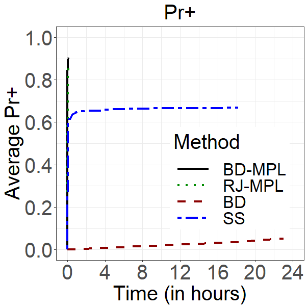
Figure 2: AUC (top-left), $Pr^{+}$ (top-right) (see Equation 15) and $Pr^{-}$ (bottom) (see Equation 16) as functions of the computational time for the cluster graph with $p=500$ and $n=5000$. The BD-MPL and RJ-MPL refers to our proposed algorithms (Algorithms 1 and 2, respectively). The SS stands for the algorithm presented by Wang (2015), while BD represents the birth-death MCMC algorithm developed by Mohammadi et al. (2023). The plot show the average over 10 replications. Note that the BD-MPL and RJ-MPL algorithm are barely visible in the $Pr-$ plot due their low running time and low $Pr-$ values.

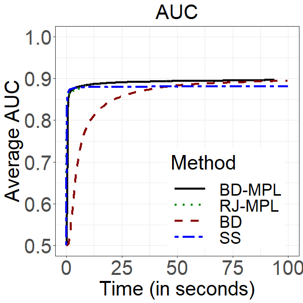
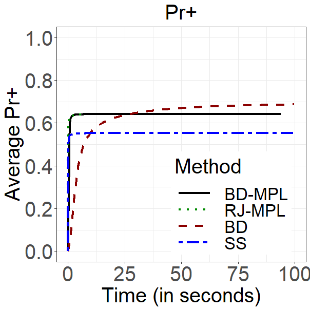
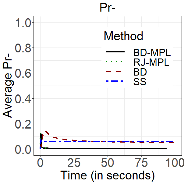
Figure 3: Average AUC (top-left), $Pr^{+}$ (top-right) (see Equation 15) and $Pr^{-}$ (bottom) (see Equation 16) as functions of the computational time for the random graph with $p=50$ and $n=500$. The BD-MPL and RJ-MPL refers to our proposed algorithms (Algorithms 1 and 2, respectively). The SS stands for the algorithm presented by Wang (2015), while BD represents the birth-death MCMC algorithm developed by Mohammadi et al. (2023). The plots show the average over 50 replications.

To highlight the distinctions in outcomes, we report three specific scenarios. Figure 1 shows the AUC as a function of the computational time for the cluster graph with a substantial number of variables and observations: $p=1000$ and $n=10000$. Both our MPL-based methods’ AUCs converge within hours, the BD-MPL method even in 2 minutes. Meanwhile, the SS algorithm takes an entire day to meet a similar AUC. The AUC of the BD algorithm remains at 0.5, even after 5 days. From Figure 2 we can draw a similar conclusion. It provides visualizations of AUC, $Pr^{+}$, and $Pr^{-}$ as a function of the computational time for the cluster graph with $p=500$ and $n=5000$. The MPL-based methods’ AUCs converge most rapidly, and their resulting $Pr^{+}$ and $Pr^{-}$ values prove to be superior. Lastly, Figure 3 presents the outcomes for the random graph when dealing with a more modest graph size, namely dimensions set at $p=50$ and $n=500$. The visualizations highlight the MPL-based algorithms’ AUC converging swiftly, though not by a striking margin compared to other algorithms. Additionally, the performance indicators $Pr^{+}$ and $Pr^{-}$ for the SS method are not on par with the other methods.

To summarize, our simulation study indicates that for large-scale graphs, specifically when $p\in\{500,1000\}$, our proposed MPL-based algorithms have outstanding computational performance compared with the alternative algorithms. Moreover, their discriminative and calibration power remains on par with other models. A notable exception are scenarios on the dense random graph, where the BD-MPL method consumes a significant amount of computational time. In practice, however, large-scale graphs with such density ($20\%$) are uncommon.

Graph	$p$	$n$	RJ-MPL	BD-MPL	BD	SS
Random	10	10	0.62	0.61	0.70	0.70
		20	0.73	0.73	0.76	0.76
		100	0.86	0.86	0.88	0.87
	50	50	0.71	0.72	0.73	0.72
		100	0.77	0.78	0.79	0.78
		500	0.88	0.90	0.91	0.88
	100	100	0.69	0.72	0.73	0.73
		200	0.75	0.78	0.79	0.78
		1000	0.86	0.89	0.90	0.88
	500	5000	0.84	0.77	0.50*	0.81
	1000	10000	0.78	0.50*	0.50*	0.79
Cluster	10	10	0.66	0.66	0.72	0.73
		20	0.76	0.78	0.79	0.79
		100	0.92	0.92	0.93	0.92
	50	50	0.82	0.83	0.85	0.84
		100	0.87	0.88	0.89	0.88
		500	0.94	0.94	0.95	0.93
	100	100	0.85	0.87	0.88	0.87
		200	0.89	0.91	0.92	0.89
		1000	0.94	0.95	0.95	0.93
	500	5000	0.98	0.98	0.77*	0.96
	1000	10000	0.98	0.99	0.52*	0.97
Scale-free	10	10	0.65	0.65	0.71	0.72
		20	0.75	0.75	0.77	0.77
		100	0.88	0.89	0.90	0.89
	50	50	0.80	0.80	0.84	0.84
		100	0.85	0.86	0.88	0.89
		500	0.93	0.94	0.95	0.94
	100	100	0.83	0.85	0.88	0.89
		200	0.87	0.89	0.91	0.91
		1000	0.93	0.95	0.95	0.95

Table 2: AUC scores per algorithm for different instances. The AUC reaches its best score at $1$ and its worst at $0$. The BD-MPL and RJ-MPL refer to our proposed algorithms (Algorithms 1 and 2, respectively). The SS stands for the algorithm presented by Wang (2015), while BD represents the birth-death MCMC algorithm developed by Mohammadi et al. (2023). The AUC values are the average over 50 replications for $p\in\{10,50,100\}$ and 10 replications for $p\in\{500,1000\}$. The best methods are boldfaced. Entries with a * indicate that the AUC had not stabilized after 5 days.

Graph	$p$	$n$	RJ-MPL	BD-MPL	BD	SS
Random	10	10	0.42	0.46	0.31	0.23
		20	0.39	0.39	0.40	0.32
		100	0.62	0.62	0.61	0.48
	50	50	0.28	0.28	0.36	0.31
		100	0.38	0.38	0.46	0.39
		500	0.64	0.64	0.70	0.55
	100	100	0.26	0.26	0.37	0.33
		200	0.37	0.37	0.47	0.42
		1000	0.62	0.63	0.71	0.58
	500	5000	0.57	0.47	0.02*	0.58
	1000	10000	0.46	0.16*	0.00*	0.53
Cluster	10	10	0.48	0.50	0.35	0.26
		20	0.47	0.47	0.44	0.37
		100	0.68	0.68	0.67	0.53
	50	50	0.47	0.47	0.50	0.44
		100	0.58	0.58	0.61	0.51
		500	0.77	0.78	0.79	0.59
	100	100	0.53	0.53	0.57	0.51
		200	0.63	0.64	0.67	0.56
		1000	0.80	0.81	0.83	0.60
	500	5000	0.86	0.90	0.29*	0.67
	1000	10000	0.79	0.92	0.02*	0.69
Scale-free	10	10	0.49	0.52	0.34	0.26
		20	0.39	0.39	0.40	0.33
		100	0.66	0.66	0.66	0.50
	50	50	0.45	0.46	0.50	0.43
		100	0.57	0.58	0.60	0.49
		500	0.79	0.79	0.81	0.56
	100	100	0.53	0.54	0.59	0.51
		200	0.65	0.66	0.69	0.55
		1000	0.82	0.83	0.85	0.58

Table 3: $Pr^{+}$ scores per algorithm for different instances. The $Pr^{+}$ (see Equation 15) reaches its best score at $1$ and its worst at $0$. The BD-MPL and RJ-MPL refers to our proposed algorithms (Algorithms 1 and 2, respectively). The SS stands for the algorithm presented by Wang (2015), while BD represents the birth-death MCMC algorithm developed by Mohammadi et al. (2023). The $Pr^{+}$ values are the average over 50 replications for $p\in\{10,50,100\}$ and 10 replications for $p\in\{500,1000\}$. The best methods are boldfaced. Entries with a * indicate that the AUC had not stabilized after 5 days.

Graph	$p$	$n$	RJ-MPL	BD-MPL	BD	SS
Random	10	10	0.29	0.33	0.15	0.12
		20	0.09	0.09	0.12	0.10
		100	0.03	0.03	0.06	0.05
	50	50	0.03	0.03	0.11	0.11
		100	0.02	0.02	0.09	0.09
		500	0.01	0.01	0.05	0.06
	100	100	0.02	0.02	0.11	0.11
		200	0.01	0.01	0.08	0.10
		1000	0.01	0.00	0.04	0.06
	500	5000	0.02	0.12	0.02*	0.18
	1000	10000	0.02	0.16*	0.00*	0.19
Cluster	10	10	0.31	0.33	0.14	0.11
		20	0.08	0.08	0.10	0.09
		100	0.03	0.03	0.04	0.04
	50	50	0.02	0.02	0.07	0.07
		100	0.01	0.01	0.05	0.05
		500	0.00	0.00	0.02	0.03
	100	100	0.01	0.01	0.05	0.06
		200	0.01	0.01	0.03	0.05
		1000	0.00	0.00	0.02	0.03
	500	5000	0.00	0.00	0.01*	0.03
	1000	10000	0.00	0.00	0.00*	0.03
Scale-free	10	10	0.33	0.37	0.16	0.13
		20	0.08	0.08	0.12	0.10
		100	0.02	0.02	0.06	0.06
	50	50	0.03	0.03	0.07	0.07
		100	0.02	0.02	0.05	0.05
		500	0.01	0.01	0.02	0.03
	100	100	0.01	0.01	0.05	0.06
		200	0.01	0.01	0.03	0.04
		1000	0.00	0.00	0.02	0.03

Table 4: $Pr^{-}$ scores per algorithm for different instances. The $Pr^{-}$ (see Equation 16) reaches its best score at $0$ and its worst at $1$. The BD-MPL and RJ-MPL refers to our proposed algorithms (Algorithms 1 and 2, respectively). The SS stands for the algorithm presented by Wang (2015), while BD represents the birth-death MCMC algorithm developed by Mohammadi et al. (2023). The $Pr^{-}$ values are the average over 50 replications for $p\in\{10,50,100\}$ and 10 replications for $p\in\{500,1000\}$. The best methods are boldfaced. Entries with a * indicate that the AUC had not stabilized after 5 days.

Graph	$p$	$n$	RJ-MPL	BD-MPL	BD	SS
Random	10	10	0.03	0.11	0.58	0.22
		20	0.01	0.05	0.49	0.20
		100	0.03	0.01	0.14	0.19
	50	50	3.17	4.59	234.25	0.98
		100	2.78	7.45	163.34	1.02
		500	1.88	13.65	117.79	1.50
	100	100	6.27	14.97	5608.53	7.17
		200	5.85	24.03	5715.78	9.37
		1000	4.57	39.97	3810.87	12.55
	500	5000	415.93	13919.92	$>$ 5 days	26823.10
	1000	10000	228873.8	$>$ 5 days	$>$ 5 days	292573.20
Cluster	10	10	0.02	0.09	0.55	0.17
		20	0.01	0.05	0.44	0.05
		100	0.01	0.01	0.22	0.07
	50	50	2.68	4.76	214.11	1.11
		100	1.81	3.00	157.55	1.10
		500	0.65	3.24	43.55	2.51
	100	100	3.33	5.88	3578.04	6.44
		200	2.66	6.82	2180.34	6.81
		1000	0.71	5.62	424.29	41.87
	500	5000	119.09	27.05	$>$ 5 days	9456.11
	1000	10000	12917.69	131.04	$>$ 5 days	84294.99
Scale-free	10	10	0.06	0.14	1.01	0.30
		20	0.02	0.06	0.27	0.10
		100	0.02	0.02	0.13	0.07
	50	50	2.47	3.35	128.92	1.39
		100	1.81	4.46	86.14	2.64
		500	1.15	4.37	63.50	4.22
	100	100	5.60	12.06	2583.78	8.84
		200	2.97	27.16	2481.84	9.93
		1000	1.22	21.37	636.93	70.66

Table 5: Time in seconds until AUC stabilization. We verify whether the AUC has stabilized by determining the minimum computational time for which the AUC differs no more than $0.01$ from the AUC value in the last iteration. The BD-MPL and RJ-MPL refers to our proposed algorithms (Algorithms 1 and 2, respectively). The SS stands for the algorithm presented by Wang (2015), while BD represents the birth-death MCMC algorithm developed by Mohammadi et al. (2023). The values shown are the average over 50 replications for $p\in\{10,50,100\}$ and 10 replications for $p\in\{500,1000\}$. The best methods are boldfaced.

5 Conclusion

We introduced two novel MCMC-based search algorithms that integrate the birth-death MCMC and reversible jump algorithms with marginal pseudo likelihood approach. These algorithms estimate the posterior distribution of the graph based on the data. It allows the exploration of the graph space instead of the joint space of graphs and precision matrices, leading to more efficient computational algorithms.

The proposed MCMC-based search algorithms behave as follows. For relatively smaller graph sizes ($p\in\{10,50,100\}$ nodes), the proposed algorithms have a similar or slightly worse AUC than state-of-the-art Bayesian structure learning methods (BD and SS). For large-scale graphs, such as $p\in\{500,1000\}$, the proposed algorithms can solve problems with high accuracy within minutes. For the cluster graph with settings $p=500$ and the number of samples $n=5000$, the MPL-based methods provide an excellent AUC within two minutes while the SS and BD methods needed 2.6 hours and more than five days, respectively. For the cluster graph with $p=1000$ and $n=10000$, the BD-MPL method had an excellent AUC within two minutes, the RJ-MPL method within 3.6 hours, the SS method within one day and the BD method after more than five days.

There are some promising lines of future research that could improve the performance of the proposed methods even further. First, the computational complexity of the BD-MPL method can be reduced substantially by leveraging parallel processing, particularly for calculating the birth and death rates. We should emphasize that even though Algorithm 1 is designed for parallel operations and is incorporated within the BDgraph package, we chose not to employ its parallel capabilities. This decision was made to preserve the reproducibility of our simulation study and to align our methods with those of other algorithms. Another potential direction is to evaluate alternative priors for the precision matrix. In Section 3.1, we employ a non-informative prior to obtain a closed form expression for the local fractional pseudo-likelihoods in Equation (7). As suggested by Leppä-Aho et al. (2017) and Consonni and Rocca (2012), we use a non-informative improper prior. Additionally, it may be worthwhile to investigate if a suitable burn-in period, alternative prior for the graph, or multiple jumps within a single iteration could help decrease computational time.

Software

The BD-MPL and RJ-MPL methods have been implemented in the R package BDgraph in the function bdgraph.mpl(), which is freely available from the Comprehensive R Archive Network (CRAN) at http://cran.r-project.org/packages=BDgraph.

References

- Albert and Barabási (2002) Albert, R. and A.-L. Barabási (2002). Statistical mechanics of complex networks. Reviews of Modern Physics 74(1), 47.
- Atay-Kayis and Massam (2005) Atay-Kayis, A. and H. Massam (2005). A Monte Carlo method for computing the marginal likelihood in nondecomposable Gaussian graphical models. Biometrika 92(2), 317–335.
- Besag (1975) Besag, J. (1975). Statistical analysis of non-lattice data. Journal of the Royal Statistical Society Series D: The Statistician 24(3), 179–195.
- Cappé et al. (2003) Cappé, O., C. Robert, and T. Rydén (2003). Reversible jump, birth-and-death and more general continuous time Markov chain Monte Carlo samplers. Journal of the Royal Statistical Society: Series B (Statistical Methodology) 65(3), 679–700.
- Carvalho and Scott (2009) Carvalho, C. M. and J. G. Scott (2009). Objective Bayesian model selection in Gaussian graphical models. Biometrika 96(3), 497–512.
- Cheng and Lenkoski (2012) Cheng, Y. and A. Lenkoski (2012). Hierarchical Gaussian graphical models: Beyond reversible jump. Electronic Journal of Statistics 6, 2309–2331.
- Consonni and Rocca (2012) Consonni, G. and L. L. Rocca (2012). Objective Bayes factors for Gaussian directed acyclic graphical models. Scandinavian Journal of Statistics 39(4), 743–756.
- Dobra et al. (2011) Dobra, A., A. Lenkoski, and A. Rodriguez (2011). Bayesian inference for general Gaussian graphical models with application to multivariate lattice data. Journal of the American Statistical Association 106(496), 1418–1433.
- Dobra and Mohammadi (2018) Dobra, A. and R. Mohammadi (2018). Loglinear model selection and human mobility. The Annals of Applied Statistics 12(2), 815–845.
- Friedman et al. (2008) Friedman, J., T. Hastie, and R. Tibshirani (2008). Sparse inverse covariance estimation with the graphical Lasso. Biostatistics 9(3), 432–441.
- Green (1995) Green, P. (1995). Reversible jump Markov chain Monte Carlo computation and Bayesian model determination. Biometrika 82(4), 711–732.
- Hanley and Mcneil (1982) Hanley, J. and B. Mcneil (1982). The meaning and use of the area under a receiver operating characteristic (roc) curve. Radiology 143(1), 29–36.
- Hinne et al. (2014) Hinne, M., A. Lenkoski, T. Heskes, and M. van Gerven (2014). Efficient sampling of Gaussian graphical models using conditional Bayes factors. Stat 3(1), 326–336.
- Ji and Seymour (1996) Ji, C. and L. Seymour (1996). A consistent model selection procedure for Markov random fields based on penalized pseudolikelihood. The Annals of Applied Probability 6(2), 423–443.
- Jones et al. (2005) Jones, B., C. Carvalho, A. Dobra, C. Hans, C. Carter, and M. West (2005). Experiments in stochastic computation for high-dimensional graphical models. Statistical Science 20(4), 388–400.
- Koller and Friedman (2009) Koller, D. and N. Friedman (2009). Probabilistic graphical models: principles and techniques. MIT press.
- Lauritzen (1996) Lauritzen, S. L. (1996). Graphical models, Volume 17. Oxford: Oxford University Press.
- Lenkoski (2013) Lenkoski, A. (2013). A direct sampler for G-Wishart variates. Stat 2(1), 119–128.
- Lenkoski and Dobra (2011) Lenkoski, A. and A. Dobra (2011). Computational aspects related to inference in Gaussian graphical models with the G-Wishart prior. Journal of Computational and Graphical Statistics 20, 140–157.
- Leppä-Aho et al. (2017) Leppä-Aho, J., J. , T. Roos, and J. Corander (2017). Learning Gaussian graphical models with fractional marginal pseudo-likelihood. International Journal of Approximate Reasoning 83, 21–42.
- Letac and Massam (2007) Letac, G. and H. Massam (2007). Wishart distributions for decomposable graphs. The Annals of Statistics 35(3), 1278–1323.
- Meinshausen and Bühlmann (2006) Meinshausen, N. and P. Bühlmann (2006). High-dimensional graphs and variable selection with the Lasso. The Annals of Statistics 34(3), 1436–1462.
- Mohammadi and Wit (2015) Mohammadi, A. and E. Wit (2015). Bayesian structure learning in sparse Gaussian graphical models. Bayesian Analysis 10(1), 109–138.
- Mohammadi (2022) Mohammadi, R. (2022). ssgraph: Bayesian graph structure learning using spike-and-slab priors. R package version 1.15.
- Mohammadi et al. (2023) Mohammadi, R., H. Massam, and G. Letac (2023). Accelerating Bayesian structure learning in sparse Gaussian graphical models. Journal of the American Statistical Association 118(542), 1345–1358.
- Mohammadi et al. (2022) Mohammadi, R., E. Wit, and A. Dobra (2022). BDgraph: Bayesian structure learning in Graphical models using birth-death MCMC. R package version 2.72.
- Niu et al. (2023) Niu, Y., Y. Ni, D. Pati, and B. K. Mallick (2023). Covariate-assisted Bayesian graph learning for heterogeneous data. Journal of the American Statistical Association (just-accepted), 1–25.
- Peng et al. (2009) Peng, J., P. Wang, N. Zhou, and J. Zhu (2009). Partial correlation estimation by joint sparse regression models. Journal of the American Statistical Association 104(486), 735–746.
- Pensar et al. (2017) Pensar, J., H. Nyman, J. Niiranen, and J. Corander (2017). Marginal pseudo-likelihood learning of discrete Markov network structures. Bayesian Analysis 12(4), 1195–1215.
- Peterson et al. (2015) Peterson, C., F. C. Stingo, and M. Vannucci (2015). Bayesian inference of multiple Gaussian graphical models. Journal of the American Statistical Association 110(509), 159–174.
- Preston (1975) Preston, C. (1975). Spatial birth-and-death processes. Bull. Inst. Inst. Stat. 46(2), 371–391.
- Ravikumar et al. (2010) Ravikumar, P., M. J. Wainwright, and J. D. Lafferty (2010). High-dimensional Ising model selection using 1-regularized logistic regression. The Annals of Statistics, 1287–1319.
- Roverato (2002) Roverato, A. (2002). Hyper inverse Wishart distribution for non-decomposable graphs and its application to Bayesian inference for Gaussian graphical models. Scandinavian Journal of Statistics 29(3), 391–411.
- Rue and Held (2005) Rue, H. and L. Held (2005). Gaussian Markov Random Fields: Theory and Applications. London: Chapman and Hall-CRC Press.
- Scutari (2013) Scutari, M. (2013). On the prior and posterior distributions used in graphical modelling. Bayesian Analysis 8(3), 505–532.
- Uhler et al. (2018) Uhler, C., A. Lenkoski, and D. Richards (2018). Exact formulas for the normalizing constants of Wishart distributions for graphical models. The Annals of Statistics 46(1), 90–118.
- van den Boom et al. (2022) van den Boom, W., A. Beskos, and M. De Iorio (2022). The G-Wishart weighted proposal algorithm: Efficient posterior computation for Gaussian graphical models. Journal of Computational and Graphical Statistics 31(4), 1215–1224.
- Vogels et al. (2023) Vogels, L., R. Mohammadi, M. Schoonhoven, and Ş. İ. Birbil (2023). Bayesian structure learning in undirected Gaussian graphical models: Literature review with empirical comparison. arXiv preprint arXiv:2307.02603.
- Wang (2012) Wang, H. (2012). The Bayesian graphical Lasso and efficient posterior computation. Bayesian Analysis 7, 771–790.
- Wang (2015) Wang, H. (2015). Scaling it up: Stochastic search structure learning in graphical models. Bayesian Analysis 10, 351–377.
- Wang and Li (2012) Wang, H. and S. Li (2012). Efficient Gaussian graphical model determination under G-Wishart prior distributions. Electronic Journal of Statistics 6, 168–198.
- Zanella (2020) Zanella, G. (2020). Informed proposals for local MCMC in discrete spaces. Journal of the American Statistical Association 115(530), 852–865.