Accelerating Inexact HyperGradient Descent for Bilevel Optimization

Abstract

We present a method for solving general nonconvex-strongly-convex bilevel optimization problems. Our method—the Restarted Accelerated HyperGradient Descent (RAHGD) method—finds an $\epsilon$-first-order stationary point of the objective with $\tilde{\mathcal{O}}(\kappa^{3.25}\epsilon^{-1.75})$ oracle complexity, where $\kappa$ is the condition number of the lower-level objective and $\epsilon$ is the desired accuracy. We also propose a perturbed variant of RAHGD for finding an $\big{(}\epsilon,\mathcal{O}(\kappa^{2.5}\sqrt{\epsilon}\,)\big{)}$-second-order stationary point within the same order of oracle complexity. Our results achieve the best-known theoretical guarantees for finding stationary points in bilevel optimization and also improve upon the existing upper complexity bound for finding second-order stationary points in nonconvex-strongly-concave minimax optimization problems, setting a new state-of-the-art benchmark. Empirical studies are conducted to validate the theoretical results in this paper.

1 Introduction

Bilevel optimization is emerging as a key unifying problem formulation in machine learning, encompassing a variety of applications including meta-learning, model-free reinforcement learning and hyperparameter optimization [16, 46]. Our work focuses on a version of the general problem that is particularly relevant to machine learning—the nonconvex-strongly-convex bilevel optimization problem:

$$\min_{x\in{\mathbb{R}}^{d_{x}}}~{}\Phi(x)\triangleq f(x,y^{*}(x)),$$ (1a)

$${\rm s.t}~{}~{}~{}~{}~{}y^{*}(x)=\operatorname*{arg\,min}_{y\in{\mathbb{R}}^{d_{y}}}~{}g(x,y),$$ (1b)

where the upper-level function $f(x,y)$ is smooth and possibly nonconvex, and the lower-level function $g(x,y)$ is smooth and strongly convex with respect to $y$ for any given $x$. Bilevel optimization is more expressive but harder to solve than classical single-level optimization since the objective $\Phi(x)$ in (1a) involves the argument input $y^{*}(x)$ which is the solution of the lower-level problem (1b). In contradistinction to classical optimization, bilevel optimization problem (1) involves solving an optimization problem where the minimization variable is taken as the minimizer of a lower-level optimization problem.

Most existing work on nonconvex-strongly-convex bilevel optimization [17, 25, 26] focuses on finding approximate first-order stationary points (FOSP) of the objective. Recently, Huang et al. [23] extended the scope of work in this area, proposing the (perturbed) approximate implicit differentiation (AID) algorithm which can find an $\big{(}\epsilon,{\mathcal{O}}(\kappa^{2.5}\sqrt{\epsilon}\,)\big{)}$-second-order stationary points (SOSP) within a $\tilde{\mathcal{O}}(\kappa^{4}\epsilon^{-2})$ oracle complexity, where $\kappa\geq 1$ is the condition number of any $f(x,\cdot)$ and $\epsilon>0$ is the desired accuracy. Given this result, a key further challenge is to study whether the $\epsilon^{-2}$-dependency in the upper complexity bound can be improved under additional Lipschitz assumptions on high-order derivatives [23].

Given this context, a natural question to ask is: Can we design an algorithm that improves upon known algorithmic complexities for finding approximate first-order and second-order stationary points in nonconvex-strongly-convex bilevel optimization?

1.1 Contributions

We resolve this question by designing a particular form of acceleration of hypergradient descent and thereby improving the oracle complexity. Our contributions are four-fold:

1. We propose a method that we refer to as Restarted Accelerated Hypergradient Descent (RAHGD) that applies Nesterov’s accelerated gradient descent (AGD) to approximate the solution $y^{*}(x)$ of the inner problem (1b) and combines it with the conjugate gradient (CG) method to construct an inexact hypergradient of the objective. The algorithm makes use of proper restarting and acceleration to optimize the objective $\Phi(\cdot)$ based on the obtained inexact hypergradient. We show that RAHGD can find an $\epsilon$-FOSP of the objective within ${\mathcal{O}}(\kappa^{3.25}\epsilon^{-1.75})$ first-order oracle queries [Section 3].

2. For the task of finding approximate second-order stationary points, we add a perturbation step to RAHGD and introduce the Perturbed Restarted Accelerated HyperGradient Descent (PRAHGD) algorithm. We show that PRAHGD can efficiently escape saddle points and find an $\big{(}\epsilon,{\mathcal{O}}(\kappa^{2.5}\sqrt{\epsilon}\,)\big{)}$-second-order stationary point of the objective $\Phi$ within $\tilde{\mathcal{O}}\big{(}\kappa^{3.25}\epsilon^{-1.75}\big{)}$ oracle queries. This improves over the best known complexity in bilevel optimization due to Huang et al. [23] by a factor of $\tilde{\mathcal{O}}(\kappa^{0.75}\epsilon^{-0.25})$ [Section 4].

3. We apply the theoretical framework of PRAHGD to the problem of minimax optimization. Specially, we propose a PRAHGD variant crafted for nonconvex-strongly-concave minimax optimization. We refer to the resulting algorithm as Perturbed Restarted Accelerate Gradient Descent Ascent (PRAGDA). We show that PRAGDA provably finds an ${\mathcal{O}}\big{(}\epsilon,{\mathcal{O}}(\kappa^{1.5}\sqrt{\epsilon}\,)\big{)}$-SOSP with a first-order oracle query complexity of $\tilde{\mathcal{O}}(\kappa^{1.75}\epsilon^{-1.75})$. This improves upon the best known first-order (including gradient/Hessian-vector/Jacobian-vector-product) oracle query complexity bound of $\tilde{\mathcal{O}}(\kappa^{1.5}\epsilon^{-2}+\kappa^{2}\epsilon^{-1.5})$ due to Luo et al. [38] [Section 5].

4. We conduct a variety of empirical studies of bilevel optimization. Specifically, we evaluate the effectiveness of our proposed algorithms (RAHGD / PRAHGD / PRAGDA) by applying them to three different tasks: a synthetic minimax problem, data hypercleaning for the MNIST dataset, and hyperparameter optimization for logistic regression. Our studies demonstrate that our algorithms outperform several established baseline algorithms, such as BA, AID-BiO, ITD-BiO, PAID-BiO and iMCN, with inevitably faster empirical convergence. The results provide empirical evidence in support of the effectiveness of our proposed algorithmic framework for bilevel and minimax optimization [Appendix E].

1.2 Overview of Our Algorithm Design and Main Techniques

We overview the algorithm design in this subsection. Inspired by the success of the accelerated gradient descent method for nonconvex optimization [see, e.g., 28, 33], we propose a novel method called the restarted accelerated hypergradient descent (RAHGD) algorithm. The gradient of $\Phi(x)$, which we called the hypergradient, can be computed via the following equation [17, 25]:

$$\nabla\Phi(x)=\nabla_{x}f(x,y^{*}(x))-\nabla^{2}_{xy}g(x,y^{*}(x))\big{(}\nabla^{2}_{yy}g(x,y^{*}(x))\big{)}^{-1}\nabla_{y}f(x,y^{*}(x)).$$ (2)

Unfortunately, directly applying first-order algorithms by iterating with the exact hypergradient $\nabla\Phi(x)$ is costly or intractable for large-scale problems, given the need to obtain $y^{*}(x)$ and particularly given the need to invert the matrix $\nabla^{2}_{yy}g(x,y^{*}(x))$.

For given $x=x_{k}\in{\mathbb{R}}^{d_{x}}$, we aim to construct an estimate of $\nabla\Phi(x_{k})$ with reasonable computational cost and sufficient accuracy. The strong convexity of $g(x_{k},\cdot)$ motivates us to apply AGD for finding $y_{k}\approx y^{*}(x_{k})$ and hence used as a replacement of arguments estimating $\nabla\Phi(x_{k})$. To avoid direct computation of the term $\big{(}\nabla^{2}_{yy}g(x_{k},y_{k})\big{)}^{-1}\nabla_{y}f(x_{k},y_{k})$, we observe that it is the solution of the following quadratic problem:

$$\min_{v\in{\mathbb{R}}^{d_{y}}}~{}\frac{1}{2}v^{\top}\nabla^{2}_{yy}g(x_{k},y_{k})v-v^{\top}\nabla_{y}f(x_{k},y_{k})$$ (3)

Accordingly, we can fastly estimate $v_{k}\approx\big{(}\nabla^{2}_{yy}g(x_{k},y_{k})\big{)}^{-1}\nabla_{y}f(x_{k},y_{k})$ and solve (3) using a conjugate gradient subroutine. Based on $y_{k}$ and $v_{k}$, we obtain the expression for an inexact hypergradient:

$$\hat{\nabla}\Phi(x_{k})=\nabla_{x}f(x_{k},y_{k})-\nabla^{2}_{xy}g(x_{k},y_{k})v_{k}$$ (4)

which can serve as a surrogate of the true hypergradient $\nabla\Phi(x_{k})$ in our first-order algorithmic design.

We formally present RAHGD in Algorithm 3. The main issue to address for RAHGD is the computational cost for achieving sufficient accuracy of $\hat{\nabla}\Phi(x_{k})$. Interestingly, our theoretical analysis shows that all of the additional cost arises from the computations of $y_{k}$ and $v_{k}$, and it can thus be bounded sharply. As a result, our algorithm can find approximate first-order stationary points with reduced oracle complexities than existing methods [17, 25]. We also introduce the perturbed RAHGD (PRAHGD) in Algorithm 3 for escaping saddle points. Extending the analysis of RAHGD, we show that PRAHGD can find approximate second-order stationary points more efficiently than existing arts [23].

1.3 Related Work

The subject of bilevel optimization problem has a long history with early work tracing back to the 1970s [5]. Recent algorithmic advances in this field have driven successful applications in areas such as meta-learning [3, 16, 24], reinforcement learning [30, 46, 21] and hyperparameter optimization [13, 44, 20].

There have also been theoretical advances in bilevel optimization in recent years. Ghadimi and Wang [17] presented a convergence rate for the AID approach when $f(x,y)$ is convex, analyzing the complexity of an accelerated algorithm that uses gradient descent to approximate $y^{*}(x_{k})$ in the inner loop and uses AGD in the outer loop. Further improvements in dependence on the condition number and analysis of the convergence were achieved via the iterative differentiation (ITD) approach by Ji et al. [25, 26], who analyzed the complexity of AID and ITD and also provided a complexicity analysis for a randomized version. Hong et al. [21] proposed the TTSA algorithm—a provable single-loop algorithm that updates two variables in an alternating manner—and presented applications to the problem of reinforcement learning under randomized scenarios. For stochastic bilevel problems, various methods have been proposed, such as BSA by Ghadimi and Wang [17], TTSA by Hong et al. [21], stocBiO by Ji et al. [25], and ALSET by Chen et al. [9]. More recent research on this front has focused on variance reduction and momentum techniques, resulting in cutting-edge stochastic first-order oracle complexities.

While much of the literature on bilevel optimization has focused on finding first-order stationary points, the problem of finding second-order stationary points has been largely unadressed. Huang et al. [23] recently proposed a perturbed algorithm for finding approximate second-order stationary points. The algorithm adopts gradient descent (GD) to approximately solve the lower-level minimization problem and conjugate gradient (CG) to solve for Hessian-vector product with GD used in the outer loop. For the problem of classical optimization, second-order methods such as those proposed in Nesterov and Polyak [40], Curtis et al. [11] have been used to obtain $\epsilon$-accurate SOSPs in single-level optimization with a complexity of ${\mathcal{O}}(\epsilon^{-1.5})$; however, they require expensive operations such as inverting Hessian matrices. A significant body of recent literature has been focusing on first-order methods for obtaining an approximate $\big{(}\epsilon,\mathcal{O}(\kappa^{2.5}\sqrt{\epsilon}\,)\big{)}$-SOSP, with the best-known query complexity of $\tilde{{\mathcal{O}}}(\epsilon^{-1.75})$ of gradient and Hessian-vector products [1, 7, 6, 27, 28, 33].

An important special case of the bilevel optimization problem (1)—the problem of minimax optimization, where $g=-f$ in Eq. (1b)—has been extensively studied in the literature (with $g=-f$ set in Eq. (1b)). Minimax optimization has been the focus of attention in the machine learning community recently due to its applications to training GANs [18, 2], to adversarial learning [19, 45] and to optimal transport [34, 22]. On the theoretically font, Nouiehed et al. [42], Jin et al. [29] studied the complexity of Multistep Gradient Descent Ascent (GDmax), and Lin et al. [35], Lu et al. [36] provided the first convergence analysis for the single-loop gradient descent ascent (GDA) algorithm. More recently, Luo et al. [37] applied the stochastic variance reduction technique to the nonconvex-strongly-concave case, achieving the first optimal complexity upper bound when $\kappa$ is treated as an $O(1)$-constant. Zhang et al. [48] proposed a stabilized smoothed GDA algorithm that achieves a better complexity for the nonconvex-concave problem. Fiez et al. [14] provided asymptotic results showing that GDA converges to a local minimax point almost surely. Nevertheless, to the best of our knowledge, all the previous works targeted finding approximate stationary points of $\Phi(x)$, and the theory for finding the local minimax points is absent in the literature. It was not until very recently that Luo et al. [38], Chen et al. [10] independently proposed (inexact) cubic-regularized Newton methods for solving this problem; these are second-order algorithms that provably converge to a local minimax point. These algorithms are limited, however, to minimax optimization and they cannot be used to solve the more general bilevel optimization problems.

Organization.

The rest of this work is organized as follows. Section 2 delineates the assumptions and specific algorithmic subroutines. Section 3 formally presents the RAHGD algorithm along with its complexity bound for finding approximation first-order stationary points. Section 4 proposes the PRAHGD, the perturbed version of RAHGD, along with its complexity bound for finding approximate second-order stationary points. Section 5 presents the application for minimax optimization. Section 6 concludes the paper and discusses future directions. Presentations of technical analysis and empirical studies are deferred to the supplementary materials.

Notation.

We let $\left\|\cdot\right\|_{2}$ be the spectral norm of matrices and the Euclidean norm of vectors. Given a real symmetric matrix $A$, we let $\lambda_{\max}(A)$ ($\lambda_{\min}(A)$) denote its largest (smallest) eigenvalue. We use the notation ${\mathbb{B}}(r)$ to present the closed Euclidean ball with radius $r$ centered at the origin. We denote $Gc(f,\epsilon)$, $JV(f,\epsilon)$ and $HV(f,\epsilon)$ as the oracle complexities of gradients, Jacobian-vector products and Hessian-vector products, respectively. Finally, we adopt the notation $\mathcal{O}(\cdot)$ to hide only absolute constants which do not depend on any problem parameters, and also $\tilde{\mathcal{O}}(\cdot)$ for constants that include a polylogarithmic factor.

Table 1: Comparison of complexities for nonconvex bilevel optimization algorithms of finding approximate FOSPs.

Algorithm	$Gc(f,\epsilon)$	$Gc(g,\epsilon)$	$JV(g,\epsilon)$	$HV(g,\epsilon)$
BA [17]	${\mathcal{O}}(\kappa^{4}\epsilon^{-2})$	${\mathcal{O}}(\kappa^{5}\epsilon^{-2.5})$	${\mathcal{O}}(\kappa^{4}\epsilon^{-2})$	$\tilde{\mathcal{O}}(\kappa^{4.5}\epsilon^{-2})$
AID-BiO [25]	${\mathcal{O}}(\kappa^{3}\epsilon^{-2})$	${\mathcal{O}}(\kappa^{4}\epsilon^{-2})$	${\mathcal{O}}(\kappa^{3}\epsilon^{-2})$	${\mathcal{O}}(\kappa^{3.5}\epsilon^{-2})$
ITD-BiO [25]	${\mathcal{O}}(\kappa^{3}\epsilon^{-2})$	$\tilde{\mathcal{O}}(\kappa^{4}\epsilon^{-2})$	$\tilde{\mathcal{O}}(\kappa^{4}\epsilon^{-2})$	$\tilde{\mathcal{O}}(\kappa^{4}\epsilon^{-2})$
RAHGD (this work)	$\tilde{\mathcal{O}}(\kappa^{2.75}\epsilon^{-1.75})$	$\tilde{\mathcal{O}}(\kappa^{3.25}\epsilon^{-1.75})$	$\tilde{\mathcal{O}}(\kappa^{2.75}\epsilon^{-1.75})$	$\tilde{\mathcal{O}}(\kappa^{3.25}\epsilon^{-1.75})$

Table 2: Comparison of complexities for nonconvex bilevel optimization algorithms of finding approximate SOSPs.

Algorithm	$Gc(f,\epsilon)$	$Gc(g,\epsilon)$	$JV(g,\epsilon)$	$HV(g,\epsilon)$
Perturbed AID [23]	$\tilde{\mathcal{O}}(\kappa^{3}\epsilon^{-2})$	$\tilde{\mathcal{O}}(\kappa^{4}\epsilon^{-2})$	$\tilde{\mathcal{O}}(\kappa^{3}\epsilon^{-2})$	$\tilde{\mathcal{O}}(\kappa^{3.5}\epsilon^{-2})$
PRAHGD (this work)	$\tilde{\mathcal{O}}(\kappa^{2.75}\epsilon^{-1.75})$	$\tilde{\mathcal{O}}(\kappa^{3.25}\epsilon^{-1.75})$	$\tilde{\mathcal{O}}(\kappa^{2.75}\epsilon^{-1.75})$	$\tilde{\mathcal{O}}(\kappa^{3.25}\epsilon^{-1.75})$

• — Notation $\tilde{\mathcal{O}}$ omits a polylogarithmic factor in relevant parameters. $\kappa$: condition number of the lower-level objective.

• — $Gc(f,\epsilon)$ and $Gc(g,\epsilon)$: number of gradient evaluations w.r.t. $f$ and $g$.

• — $JV(g,\epsilon)$: number of Jacobian-vector products $\nabla_{xy}^{2}g(x,y)v$.

• — $HV(g,\epsilon)$: number of Hessian-vector products $\nabla_{yy}^{2}g(x,y)v$.

2 Preliminaries

In this section, we first proceed to establish convergence of the algorithmic subroutines related to our algorithm—accelerated gradient descent and the conjugate gradient method. Then, we present the notations and assumptions necessary for our problem setting. We proceed to establish convergence of these two algorithmic subroutines in the following paragraphs.

Algorithm 1 ${\rm AGD}(h,z_{0},T,\alpha,\beta)$

1:  Input: objective $h(\cdot)$; initialization $z_{0}$; iteration number $T\geq 1$; step-size $\alpha>0$; momentum param. $\beta\in(0,1)$

2:  $\tilde{z}_{0}\leftarrow z_{0}$

3:  for $t=0,\dots,T-1$ do

4:   $z_{t+1}\leftarrow{\tilde{z}}_{t}-\alpha\nabla h(\tilde{z}_{t})$

5:   ${\tilde{z}}_{t+1}\leftarrow z_{t+1}+\beta(z_{t+1}-z_{t})$

6:  end for

7:  Output: $z_{T}$

Subroutine 1: Accelerated Gradient Descent.

Our first component is Nesterov’s accelerated gradient descent (AGD), which is an acceleration of the first-order method in smooth convex optimization. We describe the details of AGD for minimizing a given smooth and strongly convex function in Algorithm 1, which exhibits the following optimal convergence rate [39]:

Lemma 2.1 ([39]).

Running Algorithm 1 on an $\ell_{h}$-smooth and $\mu_{h}$-strongly convex objective function $h(\cdot)$ with $\alpha=1/\ell_{h}$ and $\beta=(\sqrt{\kappa_{h}}-1)/(\sqrt{\kappa_{h}}+1)$ produces an output $z_{T}$ satisfying

$$\|z_{T}-z^{*}\|_{2}^{2}\leq(1+\kappa_{h})\left(1-\frac{1}{\sqrt{\kappa_{h}}}\right)^{T}\|z_{0}-z^{*}\|_{2}^{2},$$

where $z^{*}=\operatorname*{arg\,min}_{z}h(z)$ and $\kappa_{h}=\ell_{h}/\mu_{h}$ denotes the condition number of the objective $h$.

Algorithm 2 ${\rm CG}(A,b,T,q_{0})$

1:  Input: quadratic objective (as in Eq. (5)); initialization $q_{0}$; iteration number $T\geq 1$

2:  $r_{0}\leftarrow Aq_{0}-b$ , $p_{0}\leftarrow-r_{0}$

3:  for $t=0,\dots,T-1$ do

4:   $\alpha_{t}\leftarrow\dfrac{r_{t}^{T}r_{t}}{p_{t}^{T}Ap_{t}}$

5:   $q_{t+1}\leftarrow q_{t}+\alpha_{t}p_{t}$

6:   $r_{t+1}\leftarrow r_{t}+\alpha_{t}Ap_{t}$

7:   $\beta_{t+1}\leftarrow\dfrac{r_{t+1}^{T}r_{t+1}}{r_{t}^{T}r_{t}}$

8:   $p_{t+1}\leftarrow-r_{t+1}+\beta_{t+1}p_{t}$

9:  end for

10:  Output: $q_{T}$

Subroutine 2: Conjugate Gradient Method.

The (linear) conjugate gradient (CG) method was proposed by Hestenes and Stiefel in the 1950s as an iterative method for solving linear systems with positive definite coefficient matrices. It serves as an alternative to Gaussian elimination that is well-suited for solving large problems. CG can be formulated as the minimization of the quadratic objective function

$$\frac{1}{2}q^{\top}Aq-q^{\top}b,$$ (5)

where $A\in{\mathbb{R}}^{d\times d}$ is a positive definite matrix and $b\in{\mathbb{R}}^{d}$ is a fixed vector. We summarize the setup of CG for minimizing function (5) in Algorithm 2, and record the following convergence property [41]:

Lemma 2.2 ([41]).

Running Algorithm 2 for minimizing quadratic function (5) produces $q_{T}$ satisfying

$$\|q_{T}-q^{*}\|_{2}\leq 2\sqrt{\kappa_{A}}\left(\dfrac{\sqrt{\kappa_{A}}-1}{\sqrt{\kappa_{A}}+1}\right)^{T}\|q_{0}-q^{*}\|_{2},$$

where $q^{*}=A^{-1}b$ denotes the unique minimizer of Eq. (5), and $\kappa_{A}=\lambda_{\max}(A)/\lambda_{\min}(A)$ denotes the condition number of (positive definite) matrix $A$.

In the rest of this section we impose the following assumptions on the upper-level function $f$ and the lower-level function $g$. We then turn to the details of our theoretical analysis:

Assumption 2.3.

The upper-level function $f(x,y)$ and lower-level function $g(x,y)$ satisfy the following conditions:

1. Function $g(x,y)$ is three times differentiable and $\mu$-strongly convex with respect to $y$ for any fixed $x$;

2. Function $f(x,y)$ is twice differentiable and $M$-Lipschitz continuous with respect to $x$ and $y$;

3. Gradient $\nabla f(x,y)$ and $\nabla g(x,y)$ are $\ell$-Lipschitz continuous with respect to $x$ and $y$;

4. Jacobian $\nabla_{xy}^{2}f(x,y)$, $\nabla_{xy}^{2}g(x,y)$ and Hessians $\nabla_{xx}^{2}f(x,y)$, $\nabla_{yy}^{2}f(x,y)$, $\nabla_{yy}^{2}g(x,y)$ are $\rho$-Lipschitz continuous with respect to $x$ and $y$;

5. Third-order derivatives $\nabla_{xyx}^{3}g(x,y),\nabla_{yxy}^{3}g(x,y)$ and $\nabla_{yyy}^{3}g(x,y)$ are $\nu$-Lipschitz continuous with respect to $x$ and $y$.

These assumptions are standard for the bilevel optimization problem we are studying. We also introduce an appropriate notion of condition number for the lower-level function $g(x,y)$.

Definition 2.4.

Under Assumption 2.3, we refer to $\kappa\triangleq\ell/\mu$ the condition number of the lower-level objective $g(x,y)$.

Leveraging such a notion, we can show that the solution to the lower-level optimization problem $y^{*}(x)=\operatorname*{arg\,min}_{y\in{\mathbb{R}}^{d_{y}}}~{}g(x,y)$ is $\kappa$-Lipschitz continuous in $x$ under Assumption 2.3, as indicated in the following lemma:

Lemma 2.5.

Suppose Assumption 2.3 holds, then $y^{*}(x)$ is $\kappa$-Lipschitz continuous, that is, we have $\left\|y^{*}(x)-y^{*}(x^{\prime})\right\|_{2}\leq\kappa\left\|x-x^{\prime}\right\|_{2}$ for any $x,x^{\prime}\in{\mathbb{R}}^{d_{x}}$.

We also can show that $\Phi(x)$ admits Lipschitz continuous gradients and Lipschitz continuous Hessians, as shown in the following lemmas:

Lemma 2.6.

Suppose Assumption 2.3 holds, then $\Phi(x)$ is $\tilde{L}$-gradient Lipschitz continuous, that is, we have $\|\nabla\Phi(x)-\nabla\Phi(x^{\prime})\|\leq\tilde{L}\|x-x^{\prime}\|$ for any $x,x^{\prime}\in{\mathbb{R}}^{d_{x}}$, where $\tilde{L}={\mathcal{O}}(\kappa^{3})$.

Lemma 2.7.

Suppose Assumption 2.3 holds, then $\Phi(x)$ is $\tilde{\rho}$-Hessian Lipschitz continuous, that is, $\|\nabla^{2}\Phi(x)-\nabla^{2}\Phi(x^{\prime})\|\leq\tilde{\rho}\|x-x^{\prime}\|$ for any $x,x^{\prime}\in{\mathbb{R}}^{d_{x}}$, where $\tilde{\rho}={\mathcal{O}}(\kappa^{5})$.

The detailed form of $\tilde{L}$ and $\tilde{\rho}$ can be found in Appendix A. We give the formal definition of an $\epsilon$-first-order stationary point as well as an $(\epsilon,\tau)$-second-order stationary point, as follows:

Definition 2.8 (Approximate First-Order Stationary Point).

Under Assumption 2.3, we call $x$ an $\epsilon$-first-order stationary point of $\Phi(x)$ if $\left\|\nabla\Phi(x)\right\|_{2}\leq\epsilon$.

Definition 2.9 (Approximate Second-Order Stationary Point).

Under Assumption 2.3, we call $x$ an $(\epsilon,\tau)$-second-order stationary point of $\Phi(x)$ if $\left\|\nabla\Phi(x)\right\|_{2}\leq\epsilon$ and $\lambda_{\min}(\nabla^{2}\Phi(x))\geq-\tau$.

We remark that these concepts are commonly used in the nonconvex optimization literature [40]. The approximate second-order stationary point is sometimes referred to as an “approximate local minimizer.”

With all these preliminaries at hand, we are ready to proceed with the (perturbed) restarted accelerated hypergradient descent method.

Algorithm 3 (Perturbed) Restarted Accelerated HyperGradient Descent, (P)RAHGD

1:  Input: initial vector $x_{0,0}$; step-size $\eta>0$; momentum parameter $\theta\in(0,1)$; parameters $\alpha>0,\beta\in(0,1)$; parameter $\{T_{t,k}\}$ of AGD; parameter $\{T_{t,k}^{\prime}\}$ of CG; iteration threshold $K\geq 1$; parameter $B$ for triggering restarting; perturbation radius $r>0$; option $\mbox{{Perturbation}}\in\{0,1\}$

2:  $k\leftarrow 0,\ t\leftarrow 0,\ x_{0,-1}\leftarrow x_{0,0},\ y_{0,-1}\leftarrow{\rm AGD}\left(g(x_{1,-1},\,\cdot\,),0,T_{0,-1},\alpha,\beta\right),\ v_{0,-1}\leftarrow y_{0,-1}$

3:  while $k<K$

4:   $w_{t,k}\leftarrow x_{t,k}+(1-\theta)(x_{t,k}-x_{t,k-1})$

5:   $y_{t,k}\leftarrow{\rm AGD}(g(w_{t,k},\,\cdot\,),y_{t,k-1},T_{t,k},\alpha,\beta)$

6:   $v_{t,k}\leftarrow{\rm CG}(\nabla^{2}_{yy}g(w_{t,k},y_{t,k}),\nabla_{y}f(w_{t,k},y_{t,k})$, $T^{\prime}_{t,k},{v_{t,k-1}})$

7:   $u_{t,k}\leftarrow\nabla_{x}f(w_{t,k},y_{t,k})-\nabla^{2}_{xy}g(w_{t,k},y_{t,k})v_{t,k}$

8:   $x_{t,k+1}\leftarrow w_{t,k}-\eta u_{t,k}$

9:   $k\leftarrow k+1$

10:   if $k\sum_{i=0}^{k-1}\|x_{t,i+1}-x_{t,i}\|^{2}>B^{2}$

11:    $v_{t+1,-1}\leftarrow v_{t,k}$

12:    $x_{t+1,0}\leftarrow\left\{\begin{array}[]{ll}x_{t,k},&\text{if~{}~{} {Perturbation}$\,=0$}\\ x_{t,k}+\xi~{}~{}\text{with}~{}~{}\xi\sim\text{Unif}({\mathbb{B}}(r)),&\text{if~{}~{} {Perturbation}$\,=1$}\end{array}\right.$

13:    $x_{t+1,-1}\leftarrow x_{t+1,0}$

14:    $k\leftarrow 0$, $t\leftarrow t+1$

15:    $y_{t,-1}\leftarrow{\rm AGD}(g(x_{t,-1},\,\cdot\,),0,T_{t,-1},\alpha,\beta)$

16:   end if

17:  end while

18:  $K_{0}\leftarrow\operatorname*{arg\,min}_{\lfloor\frac{K}{2}\rfloor\leq k\leq K-1}\left\|x_{t,k+1}-x_{t,k}\right\|_{2}$

19:  Output: $\hat{w}\leftarrow\frac{1}{K_{0}+1}\sum_{k=0}^{K_{0}}w_{t,k}$

3 Restarted Accelerated HyperGradient Descent Algorithm

In this section, we present our restarted accelerated hypergradient descent (RAHGD) algorithm and provide corresponding query complexity upper bound results. We present the details of RAHGD in Algorithm 3, which has a nested loop structure. The outer loop, indexed by $k$, uses the accelerated gradient descent method to find the solver of (1a). The AGD step in Line 5 is used to find the inexact solver of (1b). The CG step is added to compute the Hessian-vector product, as shown in (2). We note that the iteration numbers of the AGD and CG steps play an important role in the convergence analysis of Algorithm 3; moreover, at the end of this section we will show that the total iteration number of AGD and CG can be bounded sharply. Finally, note that there is a restarting step in Line 12 where the option Perturbation is taken as $\,=0$.

We let subscript $t$ index the times of restarting. We note that the subscript $t$ of epoch number is added in Algorithm 3 purely for the sake of an easier convergence analysis. The incurred storage of iterations across all epochs can be avoided when implementing Algorithm 3 in practice.

In accelerated nonconvex optimization, a straightforward application of AGD cannot ensure consistent decrements of the objective function. Inspired by the work of Li and Lin [33], we add a restarting step in Line 12—we define $\mathcal{K}$ to be the iteration number when the “if condition” triggers, and hence the iterates from $k=0$ to $k={\mathcal{K}}$ constructs one single epoch, where ${\mathcal{K}}=\min_{k}\left\{k\geq 1:\,k\sum_{t=0}^{k-1}\|x_{t+1}-x_{t}\|_{2}^{2}>B^{2}\right\}$. Then we can have the objective function consistently decrease with respect to each epoch when we run Algorithm 3. We provide the convergence results for RAHGD in the rest of this section.

Denote $v_{k}^{*}=\big{(}\nabla^{2}_{yy}g(w_{k},y_{k})\big{)}^{-1}\nabla_{y}f(w_{k},y_{k})$. Due to the bilevel optimization problem we are considering the following conditions on the inexact gradient. Recall that the overall objective function $\Phi(x)$ is $\tilde{L}$-gradient Lipschitz continuous, and both the upper-level function $f(x,y)$ and the lower-level function $g(x,y)$ are $\ell$-gradient Lipschitz continuous:

Condition 3.1.

Let $w_{-1}=x_{-1}$. Then for some $\sigma>0$, we assume that the estimators $y_{k}\in{\mathbb{R}}^{d_{y}}$ and $v_{k}\in{\mathbb{R}}^{d_{y}}$ satisfy the conditions

$$\|y_{k}-y^{*}(w_{k})\|_{2}\leq\frac{\sigma}{2\tilde{L}},\qquad\text{for each $k=-1,0,1,2,\dots$}$$ (6)

and

$$\|v_{k}-v_{k}^{*}\|\leq\frac{\sigma}{2\ell},\qquad\text{for each $k=0,1,2,\dots$}$$ (7)

Remark 3.2.

We will show at the end of this section that Condition 3.1 is guaranteed to hold after running AGD and CG for a sufficient number of iterates.

Under Condition 3.1, the bias of $\hat{\nabla}\Phi(x_{k})$ defined in equation (4) can be bounded as shown in the following lemma:

Lemma 3.3 (Inexact gradients).

Suppose Assumption 2.3 and Condition 3.1 hold, then we have $\|\nabla\Phi(w_{k})-\hat{\nabla}\Phi(w_{k})\|_{2}\leq\sigma$.

In the following theorem we show that the iteration complexity in the outer loop is bounded.

Theorem 3.4 (RAHGD finding $\epsilon$-FOSP).

Suppose that Assumptions 2.3 and Condition 3.1 hold. Let

$$\eta=\frac{1}{4\tilde{L}},\quad B=\sqrt{\frac{\epsilon}{\tilde{\rho}}},\quad\theta=4(\tilde{\rho}\epsilon\eta^{2})^{1/4},\quad K=\frac{1}{\theta},\quad\alpha=\frac{1}{\ell},\quad\beta=\frac{\sqrt{\kappa}-1}{\sqrt{\kappa}+1},\quad\sigma=\epsilon^{2}.$$

and assume that $\epsilon\leq\frac{\tilde{L}^{2}}{\tilde{\rho}}$. Denote $\Delta=\Phi(x_{\rm{int}})-\min_{x}~{}\Phi(x)$. Then RAHGD in Algorithm 3 terminates within ${\mathcal{O}}(\Delta\tilde{L}^{0.5}\tilde{\rho}^{0.25}\epsilon^{-1.75})$ iterates, outputting $\hat{w}$ satisfying $\left\|\nabla\Phi(\hat{w})\right\|_{2}\leq 83\epsilon$.

Theorem 3.4 says that Algorithm 3 can find an $\epsilon$-first-order stationary point with ${\mathcal{O}}(\kappa^{2.75}\epsilon^{-1.75})$ iterations in the outer loop. The following result indicates that Condition 3.1 holds if we run AGD and CG for a sufficient number of iterations. In addition, the total number of iterations in one epoch is at most ${\mathcal{O}}(\kappa^{0.5}{\mathcal{K}}\log(1/\epsilon))$:

Proposition 3.5.

Suppose Assumption 2.3 holds. In the $t$-th epoch, we set the inner loop iteration number $T_{t,k}$ and the CG iteration number $T_{t,k}^{\prime}$. We run Algorithm 3 with the parameter chosen in Theorem 3.4. Then all $y_{t,k}$ and $v_{t,k}$ satisfy Condition 3.1. For each $t$, we also have the following bounds for the inner loops $\sum_{k=-1}^{{\mathcal{K}}-1}T_{t,k}\leq{\mathcal{O}}(\kappa^{0.5}{\mathcal{K}}\log(1/\epsilon))$ and $\sum_{k=0}^{{\mathcal{K}}-1}T_{t,k}^{\prime}\leq{\mathcal{O}}(\kappa^{0.5}{\mathcal{K}}\log(1/\epsilon)).$

The detailed forms of $T_{t,k}$ and $T_{t,k}^{\prime}$ can be found in Appendix B. Combined with Theorem 3.4, we finally obtain the total number of oracle calls as follows:

Corollary 3.6 (Oracle complexity of RAHGD finding $\epsilon$-FOSP).

Under Assumption 2.3, we run RAHGD in Algorithm 3 with the parameters set as in Theorem 3.4 and Proposition 3.5. The output $\hat{w}$ is then an $\epsilon$-first-order stationary point of $\Phi(x)$. Additionally, the oracle complexities satisfy $Gc(f,\epsilon)=\tilde{\mathcal{O}}(\kappa^{2.75}\epsilon^{-1.75})$, $Gc(g,\epsilon)=\tilde{\mathcal{O}}(\kappa^{3.25}\epsilon^{-1.75})$, $JV(g,\epsilon)=\tilde{\mathcal{O}}(\kappa^{2.75}\epsilon^{-1.75})$ and $HV(g,\epsilon)=\tilde{\mathcal{O}}(\kappa^{3.25}\epsilon^{-1.75})$.

The algorithm can be adapted to solving the single-level nonconvex minimization problem where $\kappa$ reduces to 1, and the given complexity matches the state-of-the-art [7, 1, 6, 28, 33]. The best known lower bound in this setting is $O(\epsilon^{-1.714})$ [8]. Closing this $O(\epsilon^{-0.036})$-gap remains open even in nonconvex minimization settings.

4 Perturbed Restarted Accelerated HyperGradient Descent Algorithm

In this section, we introduce perturbation to our RAHGD algorithm. In many nonconvex problems encountered in practice in machine learning, most first-order stationary points presented are saddle points [12, 32, 27]. Recall that finding second-order stationary points require not only zero gradient, but also a positive semidefinite Hessian, a condition that certifies that we escape all saddle points successfully. Earlier work of Jin et al. [28], Li and Lin [33] shows that one can obtain an approximate second-order stationary point by intermittently perturbing the algorithm using random noise. We present the details of our perturbed restarted accelerated hypergradient descent (PRAHGD) in Algorithm 3. Compared with RAHGD, a noise-perturbation step is added in Algorithm 3 [Line 12, option Perturbation$\,=1$].

We proceed with the complexity analysis for PRAHGD, where we show that PRAHGD in Algorithm 3 outputs an $(\epsilon,\sqrt{\tilde{\rho}\epsilon}\,)$-second-order stationary point within $\tilde{\mathcal{O}}(\kappa^{3.25}\epsilon^{-1.75})$ oracle queries:

Theorem 4.1 (PRAHGD finding $(\epsilon,O(\sqrt{\epsilon}))$-SOSP).

Suppose that Assumption 2.3 and Condition 3.1 hold. We assume that $\epsilon\leq\frac{\tilde{L}^{2}}{\tilde{\rho}}$. Let

$$\chi={\mathcal{O}}\left(\log\frac{d_{x}}{\zeta\epsilon}\right),\quad\eta=\frac{1}{4\tilde{L}},\quad K=\frac{2\chi}{\theta},\quad B=\frac{1}{288\chi^{2}}\sqrt{\frac{\epsilon}{\tilde{\rho}}},\quad\theta=\frac{1}{2}(\tilde{\rho}\epsilon\eta^{2})^{1/4},\quad$$

$$\sigma=\min\left\{\dfrac{\tilde{\rho}B\zeta r\theta}{2\sqrt{d_{x}}},\epsilon^{2}\right\},\quad\alpha=\frac{1}{\ell},\quad\beta=\frac{\sqrt{\kappa}-1}{\sqrt{\kappa}+1},\quad r=\min\left\{\frac{\tilde{L}B^{2}}{4C},\frac{B+B^{2}}{\sqrt{2}},\frac{\theta B}{20K},\sqrt{\frac{\theta B^{2}}{2K}}\right\},$$

for some positive constant $C$. Denote $\Delta=\Phi(x_{\rm{int}})-\min_{x\in{\mathbb{R}}^{d_{x}}}\Phi(x)$. Then PRAHGD in Algorithm 3 terminates in at most ${\mathcal{O}}\big{(}\Delta\tilde{L}^{0.5}\tilde{\rho}^{0.25}\chi^{6}\cdot\epsilon^{-1.75}\big{)}$ iterations and the output satisfies $\left\|\nabla\Phi(\hat{w})\right\|_{2}\leq\epsilon$ and $\lambda_{\min}(\nabla^{2}\Phi(\hat{w}))\geq-1.011\sqrt{\tilde{\rho}\epsilon}$ with probability at least $1-\zeta$.

Theorem 4.1 says that PRAHGD in Algorithm 3 can find an $(\epsilon,\sqrt{\tilde{\rho}\epsilon}\,)$-second-order stationary point within $\tilde{{\mathcal{O}}}(\kappa^{2.75}\epsilon^{-1.75})$ iterations in the outer loop. The following proposition shows that Condition 3.1 holds in this setting. In addition, the total number of iterations in one epoch is at most ${\mathcal{O}}(\kappa^{0.5}\,{\mathcal{K}}\log(1/\epsilon))$:

Proposition 4.2.

Suppose Assumption 2.3 holds. In the $t$-th epoch, we set the inner loop iteration number $T_{t,k}$ and the CG iteration number $T_{t,k}^{\prime}$. We run Algorithm 3 with the parameters chosen in Theorem 4.1. Then all $y_{t,k}$ and $v_{t,k}$ satisfy the Condition 3.1. For each $t$, we also have the inner loops $\sum_{k=-1}^{{\mathcal{K}}-1}T_{t,k}\leq{\mathcal{O}}\left(\kappa^{0.5}{\mathcal{K}}\log(1/\epsilon)\right)$ and $\sum_{k=0}^{{\mathcal{K}}-1}T_{t,k}^{\prime}\leq{\mathcal{O}}\left(\kappa^{0.5}{\mathcal{K}}\log(1/\epsilon)\right)$ holds.

The detailed form of $T_{t,k}$ and $T_{t,k}^{\prime}$ can be found in Appendix C. Combining this result with Theorem 4.1, we finally obtain the total number of gradient oracle calls as follows:

Corollary 4.3 (Oracle complexity of PRAHGD finding $(\epsilon,O(\sqrt{\epsilon}))$-SOSP).

Under Assumption 2.3, we run PRAHGD in Algorithm 3 with all parameters set as in Theorem 4.1. The output $\hat{w}$ is then an $\big{(}\epsilon,\sqrt{\tilde{\rho}\epsilon}\,\big{)}$-second-order stationary point of $\Phi(x)$. Additionally, the oracle complexities satisfy that $Gc(f,\epsilon)=\tilde{\mathcal{O}}(\kappa^{2.75}\epsilon^{-1.75})$, $Gc(g,\epsilon)=\tilde{\mathcal{O}}(\kappa^{3.25}\epsilon^{-1.75})$, $JV(g,\epsilon)=\tilde{\mathcal{O}}(\kappa^{2.75}\epsilon^{-1.75})$ and $HV(g,\epsilon)=\tilde{\mathcal{O}}(\kappa^{3.25}\epsilon^{-1.75})$.

We remark that the listed query complexities are identical to the corresponding ones in Corollary 3.6 of Section 3, up to a polylogarithmic factor, indicating that the perturbed version imposes nearly no additional cost while allowing the avoidance of saddle points.

Algorithm 4 PRAGDA

1:  Input: initial vector $x_{0,0}$; step-size $\eta>0$; momentum param. $\theta\in(0,1)$; params. $\alpha>0,\beta\in(0,1),\{T_{t,k}\}$ of AGD; iteration threshold $K\geq 1$; param. $B$ for triggering restarting; perturbation radius $r>0$

2:  $k\leftarrow 0,\ t\leftarrow 0,\ x_{0,-1}\leftarrow x_{0,0}$

3:  $y_{0,-1}\leftarrow{\rm AGD}(-\bar{f}(x_{0,-1},\,\cdot\,),0,T_{0,-1},\alpha,\beta)$

4:  while $k<K$

5:   $w_{t,k}\leftarrow x_{t,k}+(1-\theta)(x_{t,k}-x_{t,k-1})$

6:   $y_{t,k}\leftarrow{\rm AGD}(-\bar{f}(w_{t,k},\,\cdot\,),y_{t,k-1},T_{t,k},\alpha,\beta)$

7:   $x_{t,k+1}\leftarrow w_{t,k}-\eta\nabla_{x}\bar{f}(w_{t,k},y_{t,k})$

8:   $k\leftarrow k+1$

9:   if $k\sum_{i=0}^{k-1}\|x_{t,i+1}-x_{t,i}\|^{2}>B^{2}$

10:    $x_{t+1,0}\leftarrow x_{t,k}+\xi,\ \xi\sim\text{Unif}({\mathbb{B}}(r))$

11:    $x_{t+1,-1}\leftarrow x_{t+1,0}$

12:    $k\leftarrow 0,\ t\leftarrow t+1$

13:    $y_{t,-1}\leftarrow{\rm AGD}(-\bar{f}(x_{t,-1},\,\cdot\,),0,T_{t,-1},\alpha,\beta)$

14:   end if

15:  end while

16:  $K_{0}\leftarrow\operatorname*{arg\,min}_{\lfloor\frac{K}{2}\rfloor\leq k\leq K-1}\left\|x_{t,k+1}-x_{t,k}\right\|_{2}$

17:  Output: $\hat{w}\leftarrow\frac{1}{K_{0}+1}\sum_{k=0}^{K_{0}}w_{t,k}$

5 Improved Convergence for Accelerating Minimax Optimization

This section applies the ideas of PRAHGD to find approximate second-order stationary points in minimax optimization problem of the form

$$\min_{x\in{\mathbb{R}}^{d_{x}}}~{}\left\{\bar{\Phi}(x)\triangleq\max_{y\in{\mathbb{R}}^{d_{y}}}\bar{f}(x,y)\right\},$$ (8)

where $\bar{f}(x,y)$ is strongly concave in $y$ but possibly nonconvex in $x$. Problems of form (8) can be regarded as a special case of a bilevel optimization problem by taking $f(x,y)=\bar{f}(x,y)$ and $g(x,y)=-\bar{f}(x,y)$. Danskin’s theorem yields $\nabla\bar{\Phi}(x)=\nabla_{x}\bar{f}(x,y^{*}(x))$, in this case, which is in fact consistent with hypergradient of form (2) with the optimality condition for the lower-level problem invoked, that is, $\nabla_{y}f(x,y^{*}(x))=0$. This implies that when applying PRAHGD to the minimax optimization problem (8), no CG subroutine is called and no Jacobian-vector or Hessian-vector product operation is invoked.

We first show in Lemma 5.1 that the minimax problem enjoys tighter Lipschitz continuouity parameters than the general bilevel problem:

Lemma 5.1.

Suppose that $\bar{f}(x,y)$ is $\ell$-smooth, $\rho$-Hessian Lipschitz continuous with respect to $x$ and $y$ and $\mu$-strongly concave in $y$ but possibly nonconvex in $x$. Then the objective $\bar{\Phi}(x)$ is $(\kappa+1)\ell$-smooth and admits $(4\sqrt{2}\kappa^{3}\rho)$-Lipschitz continuous Hessians.

We formally introduce the perturbed restarted accelerated gradient descent ascent (PRAGDA) as in Algorithm 4. Utilizing the PRAHGD complexity result as in Theorems 4.1 and 4.2 together with Lemma 5.1, we can take $\tilde{L}=(\kappa+1)\ell$ and $\tilde{\rho}=4\sqrt{2}\kappa^{3}\rho$ to conclude an improved oracle complexity upper bounds for finding second-order stationary points for this particular problem, indicated by the following result:

Theorem 5.2 (Oracle complexity of PRAGDA finding $(\epsilon,O(\sqrt{\epsilon}))$-SOSP).

Under the settings of Lemma 5.1, Algorithm 4 outputs an $\big{(}\epsilon,{\mathcal{O}}(\kappa^{1.5}\sqrt{\epsilon}\,)\big{)}$-second-order stationary point of $\bar{\Phi}(x)$ in equation (8) within $\tilde{\mathcal{O}}(\kappa^{1.75}\epsilon^{-1.75})$ gradient oracle calls.

Prior to this work, the state-of-the-art algorithm was attained by the inexact minimax cubic Newton (iMCN) method [38], which under comparable settings outputs an $\big{(}\epsilon,{\mathcal{O}}(\kappa^{1.5}\sqrt{\epsilon}\,)\big{)}$-approximate SOSP within oracle quries of $\tilde{\mathcal{O}}(\kappa^{2}\epsilon^{-1.5})$ gradients, $\tilde{\mathcal{O}}(\kappa^{1.5}\epsilon^{-2})$ Hessian-vector products and $\tilde{\mathcal{O}}(\kappa\epsilon^{-2})$ Jecobian-vector products. We compare the query complexity upper bound of PRAGDA with iMCN in detail. As can be observed, the total oracle complexity of PRAGDA is no worse than that of iMCN since $\tilde{\mathcal{O}}(\kappa^{1.75}\epsilon^{-1.75})\leq\tilde{\mathcal{O}}(\kappa^{2}\epsilon^{-1.5}+\kappa^{1.5}\epsilon^{-2})$, a simple application of AM-GM inequality. Moreover, PRAGDA only requires gradient oracle calls while iMCN additionally requires Hessian-vector and Jacobian-vector oracle calls. To summarize, PRAGDA enjoys an oracle complexity that is no inferior than that of iMCN, whereas in both of the regimes $\kappa\gg\epsilon^{-1}$ and $\kappa\ll\epsilon^{-1}$ PRAGDA’s complexity is strictly superior.

6 Discussion

We have presented the Restarted Accelerated HyperGradient Descent (RAHGD) method for solving nonconvex-strongly-convex bilevel optimization problems. Our accelerated method is able to find an $\epsilon$-first-order stationary point of the objective within $\tilde{\mathcal{O}}(\kappa^{3.25}\epsilon^{-1.75})$ oracle complexity, where $\kappa$ is the condition number of the lower-level objective and $\epsilon$ is the desired accuracy. Furthermore, we have proposed a perturbed variant of RAHGD for finding an $\big{(}\epsilon,{\mathcal{O}}(\kappa^{2.5}\sqrt{\epsilon}\,)\big{)}$-second-order stationary point within the same order of oracle complexity up to a polylogarithmic factor. As a byproduct, our algorithm variant PRAGDA improves upon the existing upper complexity bound for finding second-order stationary points in nonconvex-strongly-concave minimax optimization problems. Important directions for future research include extending our results to the nonconvex-convex setting and stochastic setting in bilevel optimization and also minimax optimization as its special case.

Appendix A Basic Lemmas

In this section, we provide some basic lemmas.

Lemma A.1.

Suppose Assumption 2.3 holds, then $y^{*}(x)$ is $\kappa$-Lipschitz continuous, that is,

$$\left\|y^{*}(x)-y^{*}(x^{\prime})\right\|_{2}\leq\kappa\left\|x-x^{\prime}\right\|_{2}$$

for any $x,x^{\prime}\in{\mathbb{R}}^{d_{x}}$.

Proof.

Recall that

$$y^{*}(x)=\arg\min_{y\in\mathbb{R}^{d_{y}}}g(x,y).$$

The optimality condition leads to $\nabla_{y}g(x,y^{*}(x))=0$ for each $x\in{\mathbb{R}}^{d_{x}}$. By taking a further derivative with respect to $x$ on both sides and applying the chain rule [43], we obtain

$$\nabla_{yx}^{2}g(x,y^{*}(x))+\nabla_{yy}^{2}g(x,y^{*}(x))\frac{\partial y^{*}(x)}{\partial x}=0.$$

The smoothness and strong convexity of $g$ in $y$ immediately indicate

$$\frac{\partial y^{*}(x)}{\partial x}=-(\nabla_{yy}^{2}g(x,y^{*}(x)))^{-1}\nabla_{yx}^{2}g(x,y^{*}(x))\ .$$

Thus we have

$$\left\|\frac{\partial y^{*}(x)}{\partial x}\right\|_{2} =\left\|(\nabla_{yy}^{2}g(x,y^{*}(x)))^{-1}\nabla_{yx}^{2}g(x,y^{*}(x))\right\|_{2}\leq\frac{\ell}{\mu}=\kappa\ ,$$

where the inequality is based on the fact that $g(x,y)$ is $\ell$-smooth with respect to $x$ and $y$ and $\mu$-strongly convex with respect to y for any $x$.

Therefore, we proved that $y^{*}(x)$ is $\kappa$-Lipschitz continuous. ∎

We also can show that $\Phi(x)$ admits Lipschitz continuous gradients and Lipschitz continuous Hessians, as shown in the following lemmas:

Lemma A.2.

Suppose Assumption 2.3 holds, then $\Phi(x)$ is $\tilde{L}$-gradient Lipschitz continuous, that is,

$$\|\nabla\Phi(x)-\nabla\Phi(x^{\prime})\|\leq\tilde{L}\|x-x^{\prime}\|$$

for any $x,x^{\prime}\in{\mathbb{R}}^{d_{x}}$, where

$$\tilde{L}=\ell+\frac{2\ell^{2}+\rho M}{\mu}+\frac{\ell^{3}+2\rho\ell M}{\mu^{2}}+\frac{\rho\ell^{2}M}{\mu^{3}}\ .$$

Proof.

Recall that

$$\nabla\Phi(x)=\nabla_{x}f(x,y^{*}(x))-\nabla^{2}_{xy}g(x,y^{*}(x))\big{(}\nabla^{2}_{yy}g(x,y^{*}(x))\big{)}^{-1}\nabla_{y}f(x,y^{*}(x))\ .$$

We denote ${\mathcal{H}}_{1}(x)=\nabla_{x}f(x,y^{*}(x))$, ${\mathcal{H}}_{2}(x)=\nabla^{2}_{xy}g(x,y^{*}(x))$, ${\mathcal{H}}_{3}(x)=\big{(}\nabla^{2}_{yy}g(x,y^{*}(x))\big{)}^{-1}$ and ${\mathcal{H}}_{4}(x)=\nabla_{y}f(x,y^{*}(x))$, then

$$\nabla\Phi(x)={\mathcal{H}}_{1}(x)-{\mathcal{H}}_{2}(x){\mathcal{H}}_{3}(x){\mathcal{H}}_{4}(x)\ .$$

We first consider ${\mathcal{H}}_{1}(x),\ {\mathcal{H}}_{2}(x)$ and ${\mathcal{H}}_{4}(x)$. For any $x,\ x^{\prime}\in\mathbb{R}^{d_{x}}$, we have

$$\|{\mathcal{H}}_{1}(x)-{\mathcal{H}}_{1}(x^{\prime})\| \leq\ell(\|x-x^{\prime}\|+\|y^{*}(x)-y^{*}(x^{\prime})\|)$$

$$\leq\ell(1+\kappa)\|x-x^{\prime}\|\ ,$$

where we use triangle inequality in the first inequality and Lemma A.2 in the second one.

We also have

$$\|{\mathcal{H}}_{2}(x)-{\mathcal{H}}_{2}(x^{\prime})\| \leq\rho(\|x-x^{\prime}\|+\|y^{*}(x)-y^{*}(x^{\prime})\|)$$

$$\leq\rho(1+\kappa)\|x-x^{\prime}\|$$

and

$$\|{\mathcal{H}}_{4}(x)-{\mathcal{H}}_{4}(x^{\prime})\| \leq\ell(\|x-x^{\prime}\|+\|y^{*}(x)-y^{*}(x^{\prime})\|)$$

$$\leq\ell(1+\kappa)\|x-x^{\prime}\|.$$

We then consider ${\mathcal{H}}_{3}(x)$. For any $x,\ x^{\prime}\in\mathbb{R}^{d_{x}}$, we have

$$\quad\|{\mathcal{H}}_{3}(x)-{\mathcal{H}}_{3}(x^{\prime})\|$$

$$=\left\|\big{(}\nabla^{2}_{yy}g(x,y^{*}(x))\big{)}^{-1}-\big{(}\nabla^{2}_{yy}g(x^{\prime},y^{*}(x^{\prime}))\big{)}^{-1}\right\|$$

$$\leq\left\|\big{(}\nabla^{2}_{yy}g(x,y^{*}(x))\big{)}^{-1}\right\|\left\|\nabla^{2}_{yy}g(x^{\prime},y^{*}(x^{\prime}))-\nabla^{2}_{yy}g(x,y^{*}(x))\right\|\left\|\big{(}\nabla^{2}_{yy}g(x^{\prime},y^{*}(x^{\prime}))\big{)}^{-1}\right\|$$

$$\leq\frac{1}{\mu^{2}}\rho(\|x-x^{\prime}\|+\|y^{*}(x)-y^{*}(x^{\prime})\|)$$

$$\leq\frac{\rho(1+\kappa)}{\mu^{2}}\|x-x^{\prime}\|\ .$$

We also have

$$\|{\mathcal{H}}_{2}(x)\|\leq\ell,\quad\|{\mathcal{H}}_{3}(x)\|\leq\frac{1}{\mu}\quad\text{and}\quad\|{\mathcal{H}}_{4}(x)\|\leq M.$$

for any $x\in\mathbb{R}^{d_{x}}$. Then for any $x,\ x^{\prime}\in\mathbb{R}^{d_{x}}$ we have

$$\quad\|\nabla\Phi(x)-\nabla\Phi(x^{\prime})\|$$

$$\leq\|{\mathcal{H}}_{1}(x)-{\mathcal{H}}_{1}(x^{\prime})\|+\|{\mathcal{H}}_{2}(x){\mathcal{H}}_{3}(x){\mathcal{H}}_{4}(x)-{\mathcal{H}}_{2}(x^{\prime}){\mathcal{H}}_{3}(x^{\prime}){\mathcal{H}}_{4}(x^{\prime})\|$$

$$\leq\ell(1+\kappa)\|x-x^{\prime}\|+\|{\mathcal{H}}_{2}(x){\mathcal{H}}_{3}(x){\mathcal{H}}_{4}(x)-{\mathcal{H}}_{2}(x){\mathcal{H}}_{3}(x){\mathcal{H}}_{4}(x^{\prime})\|$$

$$\quad+\|{\mathcal{H}}_{2}(x){\mathcal{H}}_{3}(x){\mathcal{H}}_{4}(x^{\prime})-{\mathcal{H}}_{2}(x){\mathcal{H}}_{3}(x^{\prime}){\mathcal{H}}_{4}(x^{\prime})\|$$

$$\quad+\|{\mathcal{H}}_{2}(x){\mathcal{H}}_{3}(x^{\prime}){\mathcal{H}}_{4}(x^{\prime})-{\mathcal{H}}_{2}(x^{\prime}){\mathcal{H}}_{3}(x^{\prime}){\mathcal{H}}_{4}(x^{\prime})\|$$

$$\leq\ell(1+\kappa)\|x-x^{\prime}\|+\|{\mathcal{H}}_{2}(x)\|\|{\mathcal{H}}_{3}(x)\|\|{\mathcal{H}}_{4}(x)-{\mathcal{H}}_{4}(x^{\prime})\|$$

$$\quad+\|{\mathcal{H}}_{2}(x)\|\|{\mathcal{H}}_{4}(x^{\prime})\|\|{\mathcal{H}}_{3}(x)-{\mathcal{H}}_{3}(x^{\prime})\|$$

$$\quad+\|{\mathcal{H}}_{3}(x^{\prime})\|\|{\mathcal{H}}_{4}(x^{\prime})\|\|{\mathcal{H}}_{2}(x)-{\mathcal{H}}_{2}(x^{\prime})\|$$

$$\leq\ell(1+\kappa)\|x-x^{\prime}\|+\frac{\ell^{2}}{\mu}(1+\kappa)\|x-x^{\prime}\|+\frac{\ell\rho M}{\mu^{2}}(1+\kappa)\|x-x^{\prime}\|+\frac{M\rho}{\mu}(1+\kappa)\|x-x^{\prime}\|$$

$$=\left(\ell+\frac{2\ell^{2}+\rho M}{\mu}+\frac{\ell^{3}+2\rho\ell M}{\mu^{2}}+\frac{\rho\ell^{2}M}{\mu^{3}}\right)\|x-x^{\prime}\|\ .$$

∎

Lemma A.3.

[23, Lemma 3.4]. Suppose Assumption 2.3 holds, then $\Phi(x)$ is $\tilde{\rho}$-Hessian Lipschitz continuous, that is, $\|\nabla^{2}\Phi(x)-\nabla^{2}\Phi(x^{\prime})\|\leq\tilde{\rho}\|x-x^{\prime}\|$ for any $x,x^{\prime}\in\mathbb{R}^{d_{x}}$, where

$$\tilde{\rho} =\left[\left(\rho+\frac{2\ell\rho+M\nu}{\mu}+\frac{2M\ell\nu+\rho\ell^{2}}{\mu^{2}}+\frac{M\ell^{2}\nu}{\mu^{3}}\right)\left(1+\frac{\ell}{\mu}\right)\right.$$

$$\left.\quad+\left(\frac{2\ell\rho}{\mu}+\frac{4M\rho^{2}+2\ell^{2}\rho}{\mu^{2}}+\frac{2M\ell\rho^{2}}{\mu^{3}}\right)\left(1+\frac{\ell}{\mu}\right)^{2}+\left(\frac{M\rho^{2}}{\mu^{2}}+\frac{\rho\ell}{\mu}\right)\left(1+\frac{\ell}{\mu}\right)^{3}\right]\ .$$

Lemma A.4 (Inexact gradients).

Suppose Assumption 2.3 and Condition 3.1 hold, then we have

$$\|\nabla\Phi(w_{k})-\hat{\nabla}\Phi(w_{k})\|_{2}\leq\sigma\ .$$

Proof.

Recall that

$$\nabla\Phi(x)=\nabla_{x}f(x,y^{*}(x))-\nabla^{2}_{xy}g(x,y^{*}(x))\big{(}\nabla^{2}_{yy}g(x,y^{*}(x))\big{)}^{-1}\nabla_{y}f(x,y^{*}(x))$$

and

$$\hat{\nabla}\Phi(x_{k})=\nabla_{x}f(x_{k},y_{k})-\nabla^{2}_{xy}g(x_{k},y_{k})v_{k}\ .$$

We define

$$\bar{\nabla}\Phi(x_{k})=\nabla_{x}f(x_{k},y_{k})-\nabla^{2}_{xy}g(x_{k},y_{k})\big{(}\nabla^{2}_{yy}g(x_{k},y_{k})\big{)}^{-1}\nabla_{y}f(x_{k},y_{k})\ ,$$

then we have

$$||\nabla\Phi(w_{k})-\hat{\nabla}\Phi(w_{k})||_{2} =||\nabla\Phi(w_{k})-\bar{\nabla}\Phi(w_{k})+\bar{\nabla}\Phi(w_{k})-\hat{\nabla}\Phi(w_{k})||_{2}$$

$$\leq||\nabla\Phi(w_{k})-\bar{\nabla}\Phi(w_{k})||_{2}+||\bar{\nabla}\Phi(w_{k})-\hat{\nabla}\Phi(w_{k})||_{2}$$

$$\leq\tilde{L}||y_{k}-y^{*}(w_{k})||_{2}+\ell\left|\left|v_{k}-\big{(}\nabla^{2}_{yy}g(w_{k},y_{k})\big{)}^{-1}\nabla_{y}f(w_{k},y_{k})\right|\right|_{2}$$

$$\leq\sigma\ ,$$

where we use triangle inequality in the first inequality, Lemma 2.6 and Assumption 2.3(c) in the second inequality and Condition 3.1 in the last one. ∎

Lemma A.5.

[38, Lemmas 1 and 3] Assume that $\bar{f}(x,y)$ is $\ell$-smooth, $\rho$-Hessian Lipschitz continuous with respect to $x$ and $y$ and $\mu$-strongly concave in $y$ but possibly nonconvex in $x$, then the objective $\bar{\Phi}(x)$ is $(\kappa+1)\ell$-smooth and $(4\sqrt{2}\kappa^{3}\rho)$-Hessian Lipschitz continuous.

Appendix B Proofs for Section 3

In this section, we provide the proofs for theorems in Section 3. We separate our proof into three parts. We first prove that $\Phi(x)$ decrease at least ${\mathcal{O}}(\epsilon^{3/2})$ in one epoch and thus the total number of epochs is bounded. Then we show that our RAHGD in Algorithm 3 can output an $\epsilon$-FOSP. Finally, we provide the oracle calls complexity analysis.

B.1 Proof of Theorem 3.4

To prove Theorem 3.4 we primarily consider the algorithmic behavior in a single epoch; the desired result hence follows by a simple recursive argument. We omit the subscript $t$ for notation simplicity. For each epoch except the final one, we have $1\leq{\mathcal{K}}\leq K$,

$${\mathcal{K}}\sum_{i=0}^{{\mathcal{K}}-1}\|x_{i-1}-x_{i}\|_{2}^{2}>B^{2},$$ (9)

$$\|x_{k}-x_{0}\|_{2}^{2}\leq k\sum_{i=0}^{k-1}\|x_{i+1}-x_{i}\|_{2}^{2}\leq B^{2}, \forall k<{\mathcal{K}},$$ (10)

$$\|w_{k}-x_{0}\|_{2}\leq\|x_{k}-x_{0}\|_{2}+\|x_{k}-x_{k-1}\|_{2}\leq 2B, \forall k<{\mathcal{K}},$$ (11)

$$\left\|w_{k}-w_{k-1}\right\|_{2}\leq 2B, \forall k<{\mathcal{K}},$$ (12)

where equation (12) can be proved by induction as follows. For $k=0$, we have

$$\left\|w_{0}-w_{-1}\right\|_{2}=0\leq 2B.$$

For $k=1$, we have

$$\left\|w_{1}-w_{0}\right\|_{2}=\left\|(x_{1}-x_{0})+(1-\theta)(x_{1}-x_{0})\right\|_{2}\leq 2B.$$

For $k\geq 2$, we have

$$\left\|w_{k}-w_{k-1}\right\|_{2} \leq(2-\theta)\left\|x_{k}-x_{k-1}\right\|_{2}+(1-\theta)\left\|x_{k-1}-x_{k-2}\right\|_{2}$$

$$\leq 2\sqrt{2\left\|x_{k}-x_{k-1}\right\|_{2}^{2}+2\left\|x_{k-1}-x_{k-2}\right\|_{2}^{2}}\leq 2B.$$

In the last epoch, the “if condition” does not trigger and the while loop breaks until $k=K$. Hence, we have

$$\|x_{k}-x_{0}\|_{2}^{2}\leq k\sum_{i=0}^{k-1}\|x_{i+1}-x_{i}\|_{2}^{2}\leq B^{2}, \forall k\leq K,$$ (13)

$$\|w_{k}-x_{0}\|_{2}\leq 2B, \forall k\leq K.$$ (14)

In the forthcoming, we first prepare five introductory lemmas, namely Lemmas B.1— B.5, and then prove our main Theorem 3.4. Lemma B.1 portrays how $\Phi(x)$ decreases within an epoch in the case of large gradients. When gradient is small, we utilize quadratic functions to approximate $\Phi(x)$ as shown in Lemma B.2 and Lemma B.3 and then further we introduce Lemma B.4 which illustrates how $\Phi(x)$ decrease in the small gradient case. Combining Lemma B.1 and Lemma B.4 we can introduce Lemma B.5 which shows that the total number of epochs is bounded since $\Phi(x)$ is bounded below. Finally we are ready to prove Theorem 3.4. Figure 1 shows a pictoria description of our proving process.

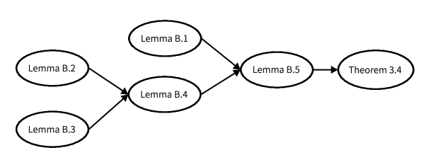
Figure 1: Proof process for Theorem 3.4

We first consider the case when $\|\nabla\Phi(w_{{\mathcal{K}}-1})\|_{2}$ is large in the following lemma.

Lemma B.1.

Suppose that Assumption 2.3 and Condition 3.1 hold. Let $\eta\leq\frac{1}{4\tilde{L}}$ and $0\leq\theta\leq 1$. When the “if condition” triggers and $\|\nabla\Phi(w_{{\mathcal{K}}-1})\|_{2}>\frac{B}{\eta}$, we have

$$\Phi(x_{\mathcal{K}})-\Phi(x_{0})\leq-\frac{B^{2}}{4\eta}+\sigma B+\frac{5\eta\sigma^{2}{\mathcal{K}}}{8}\ .$$

Proof.

Since $\Phi(x)$ has $\tilde{L}$-Lipschitz continuous gradient, we have

$$\Phi(x_{k+1}) \leq\Phi(w_{k})+\langle\nabla\Phi(w_{k}),x_{k+1}-w_{k}\rangle+\frac{\tilde{L}}{2}\|x_{k+1}-w_{k}\|_{2}^{2}$$

$$\leq\Phi(w_{k})-\eta\langle\nabla\Phi(w_{k}),\hat{\nabla}\Phi(w_{k})\rangle+\frac{\eta}{8}\|\hat{\nabla}\Phi(w_{k})\|_{2}^{2}\ ,$$

where we use $\eta\leq\frac{1}{4\tilde{L}}$. We also have

$$\Phi(x_{k})\geq\Phi(w_{k})+\langle\nabla\Phi(w_{k}),x_{k}-w_{k}\rangle-\frac{\tilde{L}}{2}\|x_{k}-w_{k}\|_{2}^{2}\ .$$

Combining above inequalities leads to

$$\quad\Phi(x_{k+1})-\Phi(x_{k})$$

$$\leq-\langle\nabla\Phi(w_{k}),x_{k}-w_{k}\rangle+\frac{\tilde{L}}{2}\|x_{k}-w_{k}\|_{2}^{2}-\eta\langle\nabla\Phi(w_{k}),\hat{\nabla}\Phi(w_{k})\rangle+\frac{\eta}{8}\|\hat{\nabla}\Phi(w_{k})\|_{2}^{2}$$

$$=\frac{1}{\eta}\langle x_{k+1}-w_{k},x_{k}-w_{k}\rangle+\langle\hat{\nabla}\Phi(w_{k})-\nabla\Phi(w_{k}),x_{k}-w_{k}\rangle+\frac{\tilde{L}}{2}\|x_{k}-w_{k}\|_{2}^{2}$$

$$\qquad\qquad-\eta\langle\nabla\Phi(w_{k}),\hat{\nabla}\Phi(w_{k})\rangle+\frac{\eta}{8}\|\hat{\nabla}\Phi(w_{k})\|_{2}^{2}$$

$$=\frac{1}{2\eta}\left(\|x_{k+1}-w_{k}\|_{2}^{2}+\|x_{k}-w_{k}\|_{2}^{2}-\|x_{k+1}-x_{k}\|_{2}^{2}\right)+\langle\hat{\nabla}\Phi(w_{k})-\nabla\Phi(w_{k}),x_{k}-w_{k}\rangle$$

$$\qquad\qquad+\frac{\tilde{L}}{2}\|x_{k}-w_{k}\|_{2}^{2}-\eta\langle\nabla\Phi(w_{k}),\hat{\nabla}\Phi(w_{k})\rangle+\frac{\eta}{8}\|\hat{\nabla}\Phi(w_{k})\|_{2}^{2}$$

$$\overset{({\rm a})}{\leq}\frac{5}{8\eta}\|x_{k}-w_{k}\|_{2}^{2}-\frac{1}{2\eta}\|x_{k+1}-x_{k}\|_{2}^{2}+\langle\hat{\nabla}\Phi(w_{k})-\nabla\Phi(w_{k}),x_{k}-w_{k}\rangle+\frac{5\eta}{8}\|\hat{\nabla}\Phi(w_{k})\|_{2}^{2}$$

$$\qquad\qquad-\eta\langle\nabla\Phi(w_{k}),\hat{\nabla}\Phi(w_{k})\rangle$$

$$\overset{({\rm b})}{\leq}\frac{5}{8\eta}\|x_{k}-x_{k-1}\|_{2}^{2}-\frac{1}{2\eta}\|x_{k+1}-x_{k}\|_{2}^{2}+\|\hat{\nabla}\Phi(w_{k})-\nabla\Phi(w_{k})\|_{2}\cdot\|x_{k}-x_{k-1}\|_{2}$$

$$\qquad\qquad+\frac{5\eta}{8}\|\hat{\nabla}\Phi(w_{k})\|_{2}^{2}-\eta\langle\nabla\Phi(w_{k}),\hat{\nabla}\Phi(w_{k})\rangle$$

$$=\frac{5}{8\eta}\|x_{k}-x_{k-1}\|_{2}^{2}-\frac{1}{2\eta}\|x_{k+1}-x_{k}\|_{2}^{2}+\|\hat{\nabla}\Phi(w_{k})-\nabla\Phi(w_{k})\|_{2}\cdot\|x_{k}-x_{k-1}\|_{2}$$

$$\qquad\qquad+\frac{5\eta}{8}\|\hat{\nabla}\Phi(w_{k})\|_{2}^{2}-\frac{\eta}{2}\left(\left\|\nabla\Phi(w_{k})\right\|_{2}^{2}+\left\|\hat{\nabla}\Phi(w_{k})\right\|_{2}^{2}-\left\|\nabla\Phi(w_{k})-\hat{\nabla}\Phi(w_{k})\right\|_{2}^{2}\right)$$

$$\overset{({\rm c})}{\leq}\frac{5}{8\eta}\|x_{k}-x_{k-1}\|_{2}^{2}-\frac{1}{2\eta}\|x_{k+1}-x_{k}\|_{2}^{2}+\|\hat{\nabla}\Phi(w_{k})-\nabla\Phi(w_{k})\|_{2}\cdot\|x_{k}-x_{k-1}\|_{2}$$

$$\qquad\qquad-\frac{3\eta}{8}\left\|\nabla\Phi(w_{k})\right\|_{2}^{2}+\frac{5\eta}{8}\left\|\nabla\Phi(w_{k})-\hat{\nabla}\Phi(w_{k})\right\|_{2}^{2}$$

$$\overset{({\rm d})}{\leq}\frac{5}{8\eta}\|x_{k}-x_{k-1}\|_{2}^{2}-\frac{1}{2\eta}\|x_{k+1}-x_{k}\|_{2}^{2}-\frac{3\eta}{8}\left\|\nabla\Phi(w_{k})\right\|_{2}^{2}+\sigma\|x_{k}-x_{k-1}\|_{2}+\frac{5\eta}{8}\sigma^{2}\ ,$$

where we use $\tilde{L}\leq\frac{1}{4\eta}$ in $\overset{({\rm a})}{\leq}$, $\left\|x_{k}-w_{k}\right\|_{2}=(1-\theta)\left\|x_{k}-x_{k-1}\right\|_{2}\leq\left\|x_{k}-x_{k-1}\right\|_{2}$ in $\overset{({\rm b})}{\leq}$, triangle inequality in $\overset{({\rm c})}{\leq}$ and Lemma 3.3 in $\overset{({\rm d})}{\leq}$.

Summing over above inequality with $k=0,1,\cdots,{\mathcal{K}}-1$ and using $x_{0}=x_{-1},$ we have

$$\quad\Phi(x_{\mathcal{K}})-\Phi(x_{0})$$ (15)

$$\leq\frac{1}{8\eta}\sum_{k=0}^{{\mathcal{K}}-2}\left\|x_{k+1}-x_{k}\right\|_{2}^{2}-\frac{3\eta}{8}\sum_{k=0}^{{\mathcal{K}}-1}\left\|\nabla\Phi(w_{k})\right\|_{2}^{2}+\sigma\sum_{k=0}^{{\mathcal{K}}-1}\left\|x_{k}-x_{k-1}\right\|_{2}+\frac{5\eta\sigma^{2}{\mathcal{K}}}{8}$$ (16)

$$\overset{({\rm e})}{\leq}\frac{1}{8\eta}\sum_{k=0}^{{\mathcal{K}}-2}\left\|x_{k+1}-x_{k}\right\|_{2}^{2}-\frac{3\eta}{8}\sum_{k=0}^{{\mathcal{K}}-1}\left\|\nabla\Phi(w_{k})\right\|_{2}^{2}+\sigma\sqrt{{\mathcal{K}}-1}\sqrt{\sum_{k=0}^{{\mathcal{K}}-2}\left\|x_{k+1}-x_{k}\right\|_{2}^{2}}+\frac{5\eta\sigma^{2}{\mathcal{K}}}{8}$$ (17)

$$\overset{({\rm f})}{\leq}\frac{B^{2}}{8\eta}-\frac{3\eta}{8}\left\|\nabla\Phi(w_{{\mathcal{K}}-1})\right\|_{2}^{2}+\sigma B+\frac{5\eta\sigma^{2}{\mathcal{K}}}{8}$$ (18)

$$\overset{({\rm g})}{\leq}-\frac{B^{2}}{4\eta}+\sigma B+\frac{5\eta\sigma^{2}{\mathcal{K}}}{8}\ ,$$ (19)

where we use Cauchy-Schwarz inequality in $\overset{({\rm e})}{\leq}$, the “if condition” in $\overset{({\rm f})}{\leq}$ and $\|\nabla\Phi(w_{{\mathcal{K}}-1})\|_{2}>\frac{B}{\eta}$ in $\overset{({\rm g})}{\leq}$. ∎

Now we consider the case when $\left\|\nabla\Phi(w_{{\mathcal{K}}-1})\right\|_{2}$ is small.

If $\left\|\nabla\Phi(w_{{\mathcal{K}}-1})\right\|_{2}\leq\frac{B}{\eta}$, then equation (11) and Lemma 3.3 lead to

$$\left\|x_{\mathcal{K}}-x_{0}\right\|_{2} \leq\left\|w_{{\mathcal{K}}-1}-x_{0}\right\|_{2}+\eta\left\|\nabla\Phi(w_{{\mathcal{K}}-1})\right\|_{2}+\eta\left\|\hat{\nabla}\Phi(w_{{\mathcal{K}}-1})-\nabla\Phi(w_{{\mathcal{K}}-1})\right\|_{2}$$

$$\leq 3B+\eta\sigma.$$

For epoch initialized at $x_{0}$, we denote ${\bf H}=\nabla^{2}\Phi(x_{0})$, and eigen-decompose it as ${\bf H}={\bf U}{\bf\Lambda}{\bf U}^{\top}$ with ${\bf\Lambda}\in{\mathbb{R}}^{d_{x}\times d_{x}}$ being orthogonal and ${\bf U}\in{\mathbb{R}}^{d_{x}\times d_{x}}$ being diagonal. Let $\lambda_{j}$ be the $j$-th eigenvalue of ${\bf H}$. We denote $\tilde{x}={\bf U}^{T}x,\tilde{w}={\bf U}^{T}w$ and $\tilde{\nabla}\Phi(w)={\bf U}^{T}\nabla\Phi(w)$. Let $\tilde{x}^{j}$ and $\tilde{\nabla}^{j}\Phi(w)$ be the $j$-th coordinate of $\tilde{x}$ and $\tilde{\nabla}\Phi(w)$, respectively. Since $\Phi$ admits $\tilde{\rho}$-Lipschitz continuous Hessian, we have

$$\Phi(x_{\mathcal{K}})-\Phi(x_{0}) \leq\langle\nabla\Phi(x_{0}),x_{\mathcal{K}}-x_{0}\rangle+\frac{1}{2}(x_{\mathcal{K}}-x_{0})^{\top}{\bf H}(x_{\mathcal{K}}-x_{0})+\frac{\tilde{\rho}}{6}\left\|x_{\mathcal{K}}-x_{0}\right\|_{2}^{3}$$ (20)

$$=\langle\tilde{\nabla}\Phi(x_{0}),\tilde{x}_{\mathcal{K}}-\tilde{x}_{0}\rangle+\frac{1}{2}(\tilde{x}_{\mathcal{K}}-\tilde{x}_{0})^{\top}{\bf\Lambda}(\tilde{x}_{\mathcal{K}}-\tilde{x}_{0})+\frac{\tilde{\rho}}{6}\left\|x_{\mathcal{K}}-x_{0}\right\|_{2}^{3}$$

$$\leq\phi(\tilde{x}_{\mathcal{K}})-\phi(\tilde{x}_{0})+\frac{\tilde{\rho}}{6}(3B+\eta\sigma)^{3},$$

where we denote

$$\phi(x)=\langle\tilde{\nabla}\Phi(x_{0}),x-\tilde{x}_{0}\rangle+\frac{1}{2}(x-\tilde{x}_{0})^{\top}{\bf\Lambda}(x-\tilde{x}_{0}),$$

and

$$\phi_{j}(x)=\langle\tilde{\nabla}^{j}\Phi(x_{0}),x-\tilde{x}_{0}^{j}\rangle+\frac{1}{2}\lambda_{j}(x-\tilde{x}_{0}^{j})^{2}.$$

Let

$$\tilde{\delta}_{k}^{j}=({\bf U}^{\top}\hat{\nabla}\Phi(w_{k}))^{j}-\nabla\phi_{j}(\tilde{w}_{k}^{j})\quad\text{and}\quad\tilde{\delta}_{k}={\bf U}^{\top}\hat{\nabla}\Phi(w_{k})-\nabla\phi(\tilde{w}_{k})\ ,$$

then the iteration of the algorithm means

$$\tilde{w}_{k}^{j}=\tilde{x}_{k}^{j}+(1-\theta)(\tilde{x}_{k}^{j}-\tilde{x}_{k-1}^{j}),$$ (21)

and

$$\tilde{x}_{k+1}^{j}=\tilde{w}_{k}^{j}-\eta({\bf U}^{\top}\hat{\nabla}\Phi(w_{k}))^{j}=\tilde{w}_{k}^{j}-\eta\nabla\phi_{j}(\tilde{w}_{k}^{j})-\eta\tilde{\delta}_{k}^{j}.$$ (22)

For any $k<{\mathcal{K}}$, we can bound $\|\tilde{\delta}_{k}\|_{2}$ as follows

$$\|\tilde{\delta}_{k}\| =\left\|{\bf U}^{\top}\hat{\nabla}\Phi(w_{k})-\tilde{\nabla}\Phi(w_{k})+\tilde{\nabla}\Phi(w_{k})-\nabla\phi(\tilde{w}_{k})\right\|_{2}$$

$$\leq\left\|\tilde{\nabla}\Phi(w_{k})-\tilde{\nabla}\Phi(x_{0})-{\bf\Lambda}(\tilde{w}_{k}-\tilde{x}_{0})\right\|_{2}+\left\|{\bf U}^{\top}\hat{\nabla}\Phi(w_{k})-\tilde{\nabla}\Phi(w_{k})\right\|_{2}$$

$$=\left\|\nabla\Phi(w_{k})-\nabla\Phi(x_{0})-{\bf H}(w_{k}-x_{0})\right\|_{2}+\left\|\hat{\nabla}\Phi(w_{k})-\nabla\Phi(w_{k})\right\|_{2}$$

$$\leq\left\|\int_{0}^{1}\langle\nabla^{2}\Phi(x_{0}+t(w_{k}-x_{0}))-{\bf H},w_{k}-x_{0}\rangle\,{\rm d}t\right\|_{2}+\sigma$$

$$\leq\frac{\tilde{\rho}}{2}\left\|w_{k}-x_{0}\right\|_{2}^{2}+\sigma$$

$$\leq 2\tilde{\rho}B^{2}+\sigma,$$

where the first inequality uses triangle inequality, the second one is based on Lemma 3.3, the third one is based on the Lipschitz continuity of Hessian, and the last one uses equation (11).
Notice that quadratic function $\phi(x)$ equals to the sum of $d_{x}$ scalar functions $\phi_{j}(x^{j})$. Then we decompose $\phi(x)$ into $\sum_{j\in S_{1}}\phi_{j}(x^{j})$ and $\sum_{j\in S_{2}}\phi_{j}(x^{j})$, where

$$S_{1}=\left\{j:\lambda_{j}\geq-\frac{\theta}{\eta}\right\}\qquad\text{and}\qquad S_{2}=\left\{j:\lambda_{j}<-\frac{\theta}{\eta}\right\}\ .$$

We first consider the term $\sum_{j\in S_{1}}\phi_{j}(x^{j})$ in the following lemma.

Lemma B.2.

Suppose that Assumption 2.3 and Condition 3.1 hold. Let $\eta\leq\frac{1}{4\tilde{L}}$ and $0\leq\theta\leq 1$. When the “if condition” triggers and $\|\nabla\Phi(w_{{\mathcal{K}}-1})\|_{2}\leq\frac{B}{\eta}$, then we have

$$\sum_{j\in S_{1}}\phi_{j}(\tilde{x}^{j}_{\mathcal{K}})-\sum_{j\in S_{1}}\phi_{j}(\tilde{x}_{0}^{j})\leq-\sum_{j\in S_{1}}\frac{3\theta}{8\eta}\sum_{k=0}^{{\mathcal{K}}-1}|\tilde{x}_{k+1}^{j}-\tilde{x}_{k}^{j}|^{2}+\frac{2\eta{\mathcal{K}}}{\theta}(2\tilde{\rho}B^{2}+\sigma)^{2}\ .$$ (23)

Proof.

Since $\phi_{j}(x)$ is quadratic, we have

$$\quad\phi_{j}(\tilde{x}_{k+1}^{j})$$

$$=\phi_{j}(\tilde{x}_{k}^{j})+\langle\nabla\phi_{j}(\tilde{x}_{k}^{j}),\tilde{x}_{k+1}^{j}-\tilde{x}_{k}^{j}\rangle+\frac{\lambda_{j}}{2}|\tilde{x}_{k+1}^{j}-\tilde{x}_{k}^{j}|^{2}$$

$$\overset{({\rm a})}{=}\phi_{j}(\tilde{x}_{k}^{j})-\frac{1}{\eta}\langle\tilde{x}_{k+1}^{j}-\tilde{w}_{k}^{j}+\eta\tilde{\delta}_{k}^{j},\tilde{x}_{k+1}^{j}-\tilde{x}_{k}^{j}\rangle+\langle\nabla\phi_{j}(\tilde{x}_{k}^{j})-\nabla\phi_{j}(\tilde{w}_{k}^{j}),\tilde{x}_{k+1}^{j}-\tilde{x}_{k}^{j}\rangle$$

$$\qquad\qquad+\frac{\lambda_{j}}{2}|\tilde{x}_{k+1}^{j}-\tilde{x}_{k}^{j}|^{2}$$

$$=\phi_{j}(\tilde{x}_{k}^{j})-\frac{1}{\eta}\langle\tilde{x}_{k+1}^{j}-\tilde{w}_{k}^{j},\tilde{x}_{k+1}^{j}-\tilde{x}_{k}^{j}\rangle-\langle\tilde{\delta}_{k}^{j},\tilde{x}_{k+1}^{j}-\tilde{x}_{k}^{j}\rangle+\lambda_{j}\langle\tilde{x}_{k}^{j}-\tilde{w}_{k}^{j},\tilde{x}_{k+1}^{j}-\tilde{x}_{k}^{j}\rangle$$

$$\qquad\qquad+\frac{\lambda_{j}}{2}|\tilde{x}_{k+1}^{j}-\tilde{x}_{k}^{j}|^{2}$$

$$=\phi_{j}(\tilde{x}_{k}^{j})+\frac{1}{2\eta}\left(|\tilde{x}_{k}^{j}-\tilde{w}_{k}^{j}|^{2}-|\tilde{x}_{k+1}^{j}-\tilde{w}_{k}^{j}|^{2}-|\tilde{x}_{k+1}^{j}-\tilde{x}_{k}^{j}|^{2}\right)-\langle\tilde{\delta}_{k}^{j},\tilde{x}_{k+1}^{j}-\tilde{x}_{k}^{j}\rangle$$

$$\qquad\qquad+\frac{\lambda_{j}}{2}\left(|\tilde{x}_{k+1}^{j}-\tilde{w}_{k}^{j}|^{2}-|\tilde{x}_{k}^{j}-\tilde{w}_{k}^{j}|^{2}\right)$$

$$\leq\phi_{j}(\tilde{x}_{k}^{j})+\frac{1}{2\eta}\left(|\tilde{x}_{k}^{j}-\tilde{w}_{k}^{j}|^{2}-|\tilde{x}_{k+1}^{j}-\tilde{w}_{k}^{j}|^{2}-|\tilde{x}_{k+1}^{j}-\tilde{x}_{k}^{j}|^{2}\right)+\frac{1}{2\alpha}|\tilde{\delta}_{k}^{j}|^{2}+\frac{\alpha}{2}|\tilde{x}_{k+1}^{j}-\tilde{x}_{k}^{j}|^{2}$$

$$\qquad\qquad+\frac{\lambda_{j}}{2}\left(|\tilde{x}_{k+1}^{j}-\tilde{w}_{k}^{j}|^{2}-|\tilde{x}_{k}^{j}-\tilde{w}_{k}^{j}|^{2}\right),$$

where we use equation (21) in $\overset{({\rm a})}{=}$.

Using the fact $\tilde{L}\geq\lambda_{j}\geq-\frac{\theta}{\eta}$ for $j\in S_{1}$ and

$$\left(-\frac{1}{2\eta}+\frac{\lambda_{j}}{2}\right)|\tilde{x}_{k+1}^{j}-\tilde{w}_{k}^{j}|^{2}\leq\left(-2\tilde{L}+\frac{\tilde{L}}{2}\right)|\tilde{x}_{k+1}^{j}-\tilde{w}_{k}^{j}|^{2}\leq 0,$$

we have

$$\quad\phi_{j}(\tilde{x}_{k+1}^{j})$$

$$\leq\phi_{j}(\tilde{x}_{k}^{j})+\frac{1}{2\eta}\left(|\tilde{x}_{k}^{j}-\tilde{w}_{k}^{j}|^{2}-|\tilde{x}_{k+1}^{j}-\tilde{x}_{k}^{j}|^{2}\right)+\frac{1}{2\alpha}|\tilde{\delta}_{k}^{j}|^{2}+\frac{\alpha}{2}|\tilde{x}_{k+1}^{j}-\tilde{x}_{k}^{j}|^{2}+\frac{\theta}{2\eta}|\tilde{x}_{k}^{j}-\tilde{w}_{k}^{j}|^{2}$$

$$\overset{({\rm b})}{=}\phi_{j}(\tilde{x}_{k}^{j})+\frac{(1-\theta)^{2}(1+\theta)}{2\eta}|\tilde{x}_{k}^{j}-\tilde{x}_{k-1}^{j}|^{2}-\left(\frac{1}{2\eta}-\frac{\alpha}{2}\right)|\tilde{x}_{k+1}^{j}-\tilde{x}_{k}^{j}|^{2}+\frac{1}{2\alpha}|\tilde{\delta}_{k}^{j}|^{2}$$

$$=\phi_{j}(\tilde{x}_{k}^{j})+\frac{(1-\theta)^{2}(1+\theta)}{2\eta}\left(|\tilde{x}_{k}^{j}-\tilde{x}_{k-1}^{j}|^{2}-|\tilde{x}_{k+1}^{j}-\tilde{x}_{k}^{j}|^{2}\right)$$

$$\qquad\qquad-\left(\frac{1}{2\eta}-\frac{\alpha}{2}-\frac{(1-\theta)^{2}(1+\theta)}{2\eta}\right)|\tilde{x}_{k+1}^{j}-\tilde{x}_{k}^{j}|^{2}+\frac{1}{2\alpha}|\tilde{\delta}_{k}^{j}|^{2}$$

$$\overset{({\rm c})}{\leq}\phi_{j}(\tilde{x}_{k}^{j})+\frac{(1-\theta)^{2}(1+\theta)}{2\eta}\left(|\tilde{x}_{k}^{j}-\tilde{x}_{k-1}^{j}|^{2}-|\tilde{x}_{k+1}^{j}-\tilde{x}_{k}^{j}|^{2}\right)-\frac{3\theta}{8\eta}|\tilde{x}_{k+1}^{j}-\tilde{x}_{k}^{j}|^{2}+\frac{2\eta}{\theta}|\tilde{\delta}_{k}^{j}|^{2}$$

for each $j\in S_{1}$, where we use equation (22) in $\overset{({\rm b})}{=}$ and let $\alpha=\frac{\theta}{4\eta}$ in $\overset{({\rm c})}{\leq}$ which leads to

$$\frac{1}{2\eta}-\frac{\alpha}{2}-\frac{(1-\theta)^{2}(1+\theta)}{2\eta}=\frac{1}{2\eta}-\frac{\theta}{8\eta}-\frac{(1-\theta)^{2}(1+\theta)}{2\eta}=\frac{3\theta}{8\eta}+\frac{\theta^{2}-\theta^{3}}{2\eta}\geq\frac{3\theta}{8\eta}.$$

Summing over above result with $k=0,1,\cdots,{\mathcal{K}}-1$ for $j\in S_{1}$ and using $x_{0}=x_{-1}$, we have

$$\quad\sum_{j\in S_{1}}\phi_{j}(\tilde{x}_{{\mathcal{K}}}^{j})$$

$$\leq\sum_{j\in S_{1}}\phi_{j}(\tilde{x}_{0}^{j})-\sum_{j\in S_{1}}\frac{3\theta}{8\eta}\sum_{k=0}^{{\mathcal{K}}-1}|\tilde{x}_{k+1}^{j}-\tilde{x}_{k}^{j}|^{2}+\frac{2\eta}{\theta}\sum_{k=0}^{{\mathcal{K}}-1}\left\|\tilde{\delta}_{k}\right\|_{2}^{2}-\frac{(1-\theta)^{2}(1+\theta)}{2\eta}|\tilde{x}_{\mathcal{K}}^{j}-\tilde{x}_{{\mathcal{K}}-1}^{j}|^{2}$$

$$\leq\sum_{j\in S_{1}}\phi_{j}(\tilde{x}_{0}^{j})-\sum_{j\in S_{1}}\frac{3\theta}{8\eta}\sum_{k=0}^{{\mathcal{K}}-1}|\tilde{x}_{k+1}^{j}-\tilde{x}_{k}^{j}|+\frac{2\eta{\mathcal{K}}}{\theta}(2\tilde{\rho}B^{2}+\sigma)^{2}.$$

This completes the proof. ∎

Next, we consider the term $\sum_{j\in S_{2}}\phi_{j}(x^{j})$.

Lemma B.3.

Suppose that Assumption 2.3 and Condition 3.1 hold. Let $\eta\leq\frac{1}{4\tilde{L}}$ and $0\leq\theta\leq 1$. When the “if condition” triggers and $\|\nabla\Phi(w_{{\mathcal{K}}-1})\|_{2}\leq\frac{B}{\eta}$, then we have

$$\sum_{j\in S_{2}}\phi_{j}(\tilde{x}^{j}_{\mathcal{K}})-\sum_{j\in S_{2}}\phi_{j}(\tilde{x}_{0}^{j})\leq-\sum_{j\in S_{2}}\frac{\theta}{2\eta}\sum_{k=0}^{{\mathcal{K}}-1}|\tilde{x}_{k+1}^{j}-\tilde{x}_{k}^{j}|^{2}+\frac{\eta{\mathcal{K}}}{2\theta}(2\tilde{\rho}B^{2}+\sigma)^{2}+\frac{\eta{\mathcal{K}}}{2\theta}\sigma^{2}\ .$$ (24)

Proof.

We denote $\nu_{j}=\tilde{x}_{0}^{j}-\frac{1}{\lambda_{j}}\tilde{\nabla}^{j}\Phi(x_{0})$, then $\phi_{j}(x)$ can be rewritten as

$$\phi_{j}(x) =\frac{\lambda_{j}}{2}\left(x-\tilde{x}_{0}^{j}+\frac{1}{\lambda_{j}}\tilde{\nabla}^{j}\Phi(x_{0})\right)^{2}-\frac{1}{2\lambda_{j}}|\tilde{\nabla}^{j}\Phi(x_{0})|^{2}=\frac{\lambda_{j}}{2}(x-\nu_{j})^{2}-\frac{1}{2\lambda_{j}}|\tilde{\nabla}^{j}\Phi(x_{0})|^{2}\ .$$

For each $j\in S_{2}=\{j:\lambda_{j}<-\frac{\theta}{\eta}\}$, we have

$$\phi_{j}(\tilde{x}_{k+1}^{j})-\phi_{j}(\tilde{x}_{k}^{j}) =\frac{\lambda_{j}}{2}|\tilde{x}_{k+1}^{j}-\nu_{j}|^{2}-\frac{\lambda_{j}}{2}|\tilde{x}_{k}^{j}-\nu_{j}|^{2}$$ (25)

$$=\frac{\lambda_{j}}{2}|\tilde{x}_{k+1}^{j}-\tilde{x}_{k}^{j}|^{2}+\lambda_{j}\langle\tilde{x}_{k+1}^{j}-\tilde{x}_{k}^{j},\tilde{x}_{k}^{j}-\nu_{j}\rangle$$

$$\leq-\frac{\theta}{2\eta}|\tilde{x}_{k+1}^{j}-\tilde{x}_{k}^{j}|^{2}+\lambda_{j}\langle\tilde{x}_{k+1}^{j}-\tilde{x}_{k}^{j},\tilde{x}_{k}^{j}-\nu_{j}\rangle\ .$$

So we only need to bound the second part. From equation (21) and equation (22), we have

$$\tilde{x}_{k+1}^{j}-\tilde{x}_{k}^{j} =\tilde{w}_{k}^{j}-\tilde{x}_{k}^{j}-\eta\nabla\phi_{j}(\tilde{w}_{k}^{j})-\eta\tilde{\delta}_{k}^{j}$$

$$=(1-\theta)(\tilde{x}_{k}^{j}-\tilde{x}_{k-1}^{j})-\eta\lambda_{j}(\tilde{w}_{k}^{j}-\nu_{j})-\eta\tilde{\delta}_{k}^{j}$$

$$=(1-\theta)(\tilde{x}_{k}^{j}-\tilde{x}_{k-1}^{j})-\eta\lambda_{j}(\tilde{x}_{k}^{j}-\nu_{j}+(1-\theta)(\tilde{x}_{k}^{j}-\tilde{x}_{k-1}^{j}))-\eta\tilde{\delta}_{k}^{j}\ .$$

So for each $j\in S_{2}$, we have

$$\small\begin{split}&\quad\langle\tilde{x}_{k+1}^{j}-\tilde{x}_{k}^{j},\tilde{x}_{k}^{j}-\nu_{j}\rangle\\ &=(1-\theta)\langle\tilde{x}_{k}^{j}-\tilde{x}_{k-1}^{j},\tilde{x}_{k}^{j}-\nu_{j}\rangle-\eta\lambda_{j}|\tilde{x}_{k}^{j}-\nu_{j}|^{2}-\eta\lambda_{j}(1-\theta)\langle\tilde{x}_{k}^{j}-\tilde{x}_{k-1}^{j},\tilde{x}_{k}^{j}-\nu_{j}\rangle-\eta\langle\tilde{\delta}_{k}^{j},\tilde{x}_{k}^{j}-\nu_{j}\rangle\\ &\geq(1-\theta)\langle\tilde{x}_{k}^{j}-\tilde{x}_{k-1}^{j},\tilde{x}_{k}^{j}-\nu_{j}\rangle-\eta\lambda_{j}|\tilde{x}_{k}^{j}-\nu_{j}|^{2}\\ &\qquad+\frac{\eta\lambda_{j}(1-\theta)}{2}(|\tilde{x}_{k}^{j}-\tilde{x}_{k-1}^{j}|^{2}+|\tilde{x}_{k}^{j}-\nu_{j}|^{2})+\frac{\eta}{2\lambda_{j}(1+\theta)}|\tilde{\delta}_{k}^{j}|^{2}+\frac{\eta\lambda_{j}(1+\theta)}{2}|\tilde{x}_{k}^{j}-\nu_{j}|^{2}\\ &=(1-\theta)\langle\tilde{x}_{k}^{j}-\tilde{x}_{k-1}^{j},\tilde{x}_{k}^{j}-\nu_{j}\rangle+\frac{\eta\lambda_{j}(1-\theta)}{2}|\tilde{x}_{k}^{j}-\tilde{x}_{k-1}^{j}|^{2}+\frac{\eta}{2\lambda_{j}(1+\theta)}|\tilde{\delta}_{k}^{j}|^{2}\\ &=(1-\theta)\langle\tilde{x}_{k}^{j}-\tilde{x}_{k-1}^{j},\tilde{x}_{k-1}^{j}-\nu_{j}\rangle+(1-\theta)|\tilde{x}_{k}^{j}-\tilde{x}_{k-1}^{j}|^{2}+\frac{\eta\lambda_{j}(1-\theta)}{2}|\tilde{x}_{k}^{j}-\tilde{x}_{k-1}^{j}|^{2}+\frac{\eta}{2\lambda_{j}(1+\theta)}|\tilde{\delta}_{k}^{j}|^{2}\\ &\geq(1-\theta)\langle\tilde{x}_{k}^{j}-\tilde{x}_{k-1}^{j},\tilde{x}_{k-1}^{j}-\nu_{j}\rangle+\frac{\eta}{2\lambda_{j}}|\tilde{\delta}_{k}^{j}|^{2}\ ,\end{split}$$

where we use the fact that $\lambda_{j}<0$ when $j\in S_{2}$ in the first inequality and the fact

$$\left(1+\frac{\eta\lambda_{j}}{2}\right)(1-\theta)\geq\left(1-\frac{\eta\tilde{L}}{2}\right)(1-\theta)\geq 0$$

indicates the second inequality. Then we have

$$\small\begin{split}&~{}~{}~{}~{}\langle\tilde{x}_{k+1}^{j}-\tilde{x}_{k}^{j},\tilde{x}_{k}^{j}-\nu_{j}\rangle\\ &\geq(1-\theta)^{k}\langle\tilde{x}_{1}^{j}-\tilde{x}_{0}^{j},\tilde{x}_{0}^{j}-\nu_{j}\rangle+\frac{\eta}{2\lambda_{j}}\sum_{i=1}^{k}(1-\theta)^{k-i}|\tilde{\delta}_{i}^{j}|^{2}\\ &\overset{({\rm a})}{=}-\frac{\eta}{2\lambda_{j}}(1-\theta)^{k}\langle\nabla^{j}\Phi(x_{0}),\hat{\nabla}^{j}\Phi(x_{0})\rangle+\frac{\eta}{2\lambda_{j}}\sum_{i=1}^{k}(1-\theta)^{k-i}|\tilde{\delta}_{i}^{j}|^{2}\\ &=-\frac{\eta}{2\lambda_{j}}(1-\theta)^{k}\left(|\nabla^{j}\Phi(x_{0})|^{2}+|\hat{\nabla}^{j}\Phi(x_{0})|^{2}-|\nabla^{j}\Phi(x_{0})-\hat{\nabla}^{j}\Phi(x_{0})|^{2}\right)+\frac{\eta}{2\lambda_{j}}\sum_{i=1}^{k}(1-\theta)^{k-i}|\tilde{\delta}_{i}^{j}|^{2}\\ &\overset{({\rm b})}{\geq}\frac{\eta}{2\lambda_{j}}(1-\theta)^{k}\left(|\nabla^{j}\Phi(x_{0})-\hat{\nabla}^{j}\Phi(x_{0})|^{2}\right)+\frac{\eta}{2\lambda_{j}}\sum_{i=1}^{k}(1-\theta)^{k-i}|\tilde{\delta}_{i}^{j}|^{2},\end{split}$$

where we use

$$\tilde{x}_{1}^{j}-\tilde{x}_{0}^{j}=\tilde{x}_{1}^{j}-\tilde{w}_{0}^{j}=-\eta\left({\bf U}^{\top}\hat{\nabla}\Phi(x_{0})\right)^{j}\quad\text{and}\quad\tilde{x}_{0}^{j}-\nu_{j}=-\frac{1}{\lambda_{j}}\tilde{\nabla}^{j}\Phi(x_{0})$$

in $\overset{(\rm{a})}{=}$ and $\lambda_{j}<0$ in $\overset{({\rm b})}{\geq}$. Plugging above inequality into equation (25) and using $\lambda_{j}<0$, we have

$$\small\begin{split}\phi_{j}(\tilde{x}_{k+1}^{j})-\phi_{j}(\tilde{x}_{k}^{j})&\leq-\frac{\theta}{2\eta}|\tilde{x}_{k+1}^{j}-\tilde{x}_{k}^{j}|^{2}+\frac{\eta}{2}(1-\theta)^{k}\left(|\nabla^{j}\Phi(x_{0})-\hat{\nabla}^{j}\Phi(x_{0})|^{2}\right)+\frac{\eta}{2}\sum_{i=1}^{k}(1-\theta)^{k-i}|\tilde{\delta}_{i}^{j}|^{2}.\end{split}$$

Summing over above result with $k=0,1,\dots,{\mathcal{K}}-1$ for $j\in S_{2}$, we have

$$\quad\sum_{j\in S_{2}}\phi_{j}(\tilde{x}^{j}_{\mathcal{K}})-\sum_{j\in S_{2}}\phi_{j}(\tilde{x}_{0}^{j})$$

$$\leq-\sum_{j\in S_{2}}\frac{\theta}{2\eta}\sum_{k=0}^{{\mathcal{K}}-1}|\tilde{x}_{k+1}^{j}-\tilde{x}_{k}^{j}|^{2}+\frac{\eta}{2}\left\|\nabla\Phi(x_{0})-\hat{\nabla}\Phi(x_{0})\right\|_{2}^{2}\sum_{k=0}^{{\mathcal{K}}-1}(1-\theta)^{k}+\frac{\eta}{2}\sum_{k=0}^{{\mathcal{K}}-1}\sum_{i=1}^{k}(1-\theta)^{k-i}\|\tilde{\delta}_{i}\|_{2}^{2}$$

$$\leq-\sum_{j\in S_{2}}\frac{\theta}{2\eta}\sum_{k=0}^{{\mathcal{K}}-1}|\tilde{x}_{k+1}^{j}-\tilde{x}_{k}^{j}|^{2}+\frac{\eta}{2}\sigma^{2}\sum_{k=0}^{{\mathcal{K}}-1}(1-\theta)^{k}+\frac{\eta}{2}\sum_{k=0}^{{\mathcal{K}}-1}\sum_{i=1}^{k}(1-\theta)^{k-i}\|\tilde{\delta}_{i}\|_{2}^{2}$$

$$\leq-\sum_{j\in S_{2}}\frac{\theta}{2\eta}\sum_{k=0}^{{\mathcal{K}}-1}|\tilde{x}_{k+1}^{j}-\tilde{x}_{k}^{j}|^{2}+\frac{\eta{\mathcal{K}}}{2\theta}\sigma^{2}+\frac{\eta{\mathcal{K}}}{2\theta}(2\tilde{\rho}B+\sigma)^{2},$$

which completes the proof. ∎

Putting Lemmas B.2 and  B.3 together we can lower bound the decrement of $\Phi(x)$ in a single epoch.

Lemma B.4.

Suppose that Assumption 2.3 and Condition 3.1 hold. Let $\eta\leq\frac{1}{4\tilde{L}}$ and $0\leq\theta\leq 1$. When the “if condition” triggers and $\|\nabla\Phi(w_{{\mathcal{K}}-1})\|_{2}\leq\frac{B}{\eta}$, we have

$$\Phi(x_{\mathcal{K}})-\Phi(x_{0})\leq-\frac{\epsilon^{3/2}}{\sqrt{\tilde{\rho}}}\ .$$

Proof.

Summing over equation (23) and equation (24), we have

$$\phi(\tilde{x}_{\mathcal{K}})-\phi(\tilde{x}_{0}) =\sum_{j\in S_{1}\cup S_{2}}\phi_{j}(\tilde{x}_{\mathcal{K}}^{j})-\phi_{j}(\tilde{x}_{0}^{j})$$ (26)

$$\leq\frac{3\theta}{8\eta}\sum_{k=0}^{{\mathcal{K}}-1}\left\|\tilde{x}_{k+1}-\tilde{x}_{k}\right\|_{2}^{2}+\frac{5\eta{\mathcal{K}}}{2\theta}(2\tilde{\rho}B^{2}+\sigma)^{2}+\frac{\eta{\mathcal{K}}}{2\theta}\sigma^{2}$$

$$\leq-\frac{3\theta B^{2}}{8\eta{\mathcal{K}}}+\frac{5\eta{\mathcal{K}}}{2\theta}(2\tilde{\rho}B^{2}+\sigma)^{2}+\frac{\eta{\mathcal{K}}}{2\theta}\sigma^{2},$$

where we use equation (9) in the last inequality. Plugging into equation (20) and using ${\mathcal{K}}\leq K$, we have

$$\Phi(x_{\mathcal{K}})-\Phi(x_{0}) \leq-\frac{3\theta B^{2}}{8\eta{\mathcal{K}}}+\frac{5\eta{\mathcal{K}}}{2\theta}(2\tilde{\rho}B^{2}+\sigma)^{2}+\frac{\tilde{\rho}}{6}(3B+\eta\sigma)^{3}+\frac{\eta{\mathcal{K}}}{2\theta}\sigma^{2}$$ (27)

$$\leq-\frac{3\theta B^{2}}{8\eta K}+\frac{5\eta K}{2\theta}(2\tilde{\rho}B^{2}+\sigma)^{2}+\frac{\tilde{\rho}}{6}(3B+\eta\sigma)^{3}+\frac{\eta{\mathcal{K}}}{2\theta}\sigma^{2}$$

$$\leq-\frac{\epsilon^{3/2}}{\sqrt{\tilde{\rho}}}\ .$$

This completes the proof. ∎

Now we can provide an upper bound on the total number of epochs, as shown in the following lemma.

Lemma B.5.

Consider the setting of Theorem 3.4, and we run RAHGD in Algorithm 3. Then the algorithm terminates in at most $\Delta\sqrt{\tilde{\rho}}\epsilon^{-3/2}$ epochs.

Proof of Lemma B.5.

From Lemma B.1 and  B.4, we have

$$\Phi(x_{\mathcal{K}})-\Phi(x_{0})\leq-\min\left\{\frac{\epsilon^{3/2}}{\sqrt{\tilde{\rho}}},\frac{\epsilon\tilde{L}}{\tilde{\rho}}\right\}\ .$$ (28)

Notice that in Algorithm 3, we set $x_{0}$ to be the last iterate $x_{{\mathcal{K}}}$ in the previous epoch. Suppose the total number of epochs $N>\Delta\sqrt{\tilde{\rho}}\epsilon^{-3/2}$, then summing over all epochs we have

$$\min_{x\in{\mathbb{R}}^{d_{x}}}\Phi(x)-\Phi(x_{\rm{int}})\leq-N\min\left\{\frac{\epsilon^{3/2}}{\sqrt{\tilde{\rho}}},\frac{\epsilon\tilde{L}}{\tilde{\rho}}\right\}<-\Delta,$$ (29)

leading to contradiction. Therefore the algorithm terminates in at most $\Delta\sqrt{\tilde{\rho}}\epsilon^{-3/2}$ epochs. ∎

We are now prepared to finish the proof of Theorem 3.4.

Proof of Theorem 3.4.

Lemma B.5 says that RAHGD will terminate in at most $\Delta\sqrt{\tilde{\rho}}\epsilon^{-3/2}$ epochs. Since each epoch needs at most $K=\frac{1}{2}\big{(}\tilde{L}^{2}/(\tilde{\rho}\epsilon)\big{)}^{1/4}$ iterations, the total iterations must be less than $\Delta\tilde{L}^{1/2}\tilde{\rho}^{1/4}\epsilon^{-7/4}$. Recall that we have $\tilde{L}={\mathcal{O}}(\kappa^{3})$ and $\tilde{\rho}={\mathcal{O}}(\kappa^{5})$, thus the total iterations is at most ${\mathcal{O}}(\kappa^{11/4}\epsilon^{-7/4})$.
Now we consider the last epoch. Denote $\tilde{w}={\bf U}^{\top}\hat{w}=\frac{1}{K_{0}+1}\sum_{k=0}^{K_{0}}{\bf U}^{\top}w_{k}=\frac{1}{K_{0}+1}\sum_{k=0}^{K_{0}}\tilde{w}_{k}$. Since $\phi$ is quadratic, we have

$$\left\|\phi(\tilde{w})\right\|_{2} =\left\|\frac{1}{K_{0}+1}\sum_{k=0}^{K_{0}}\nabla\phi(\tilde{w}_{k})\right\|_{2}$$

$$\overset{({\rm a})}{=}\frac{1}{\eta(K_{0}+1)}\left\|\sum_{k=0}^{K_{0}}\left(\tilde{x}_{k+1}-\tilde{w}_{k}+\eta\tilde{\delta}_{k}\right)\right\|_{2}$$

$$=\frac{1}{\eta(K_{0}+1)}\left\|\sum_{k=0}^{K_{0}}\left(\tilde{x}_{k+1}-\tilde{x}_{k}-(1-\theta)(\tilde{x}_{k}-\tilde{x}_{k-1})+\eta\tilde{\delta}_{k}\right)\right\|_{2}$$

$$\overset{({\rm b})}{=}\frac{1}{\eta(K_{0}+1)}\left\|\tilde{x}_{K_{0}+1}-\tilde{x}_{0}-(1-\theta)(\tilde{x}_{K_{0}}-\tilde{x}_{0}+\eta\sum_{k=0}^{K_{0}}\tilde{\delta}_{k}\right\|_{2}$$

$$=\frac{1}{\eta(K_{0}+1)}\left\|\tilde{x}_{K_{0}+1}-\tilde{x}_{K_{0}}+\theta(\tilde{x}_{K_{0}}-\tilde{x}_{0})+\eta\sum_{k=0}^{K_{0}}\tilde{\delta}_{k}\right\|_{2}$$

$$\leq\frac{1}{\eta(K_{0}+1)}\left(\left\|\tilde{x}_{K_{0}+1}-\tilde{x}_{K_{0}}\right\|_{2}+\theta\left\|\tilde{x}_{K_{0}}-\tilde{x}_{0}\right\|_{2}+\eta\sum_{k=0}^{K_{0}}\left\|\tilde{\delta}_{k}\right\|_{2}\right)$$

$$\overset{({\rm c})}{\leq}\frac{2}{\eta K}\left\|\tilde{x}_{K_{0}+1}-\tilde{x}_{K_{0}}\right\|_{2}+\frac{2\theta B}{\eta K}+2\tilde{\rho}B^{2}+\sigma,$$

where we use equation (22) in $\overset{({\rm a})}{=}$, $x_{-1}=x_{0}$ in $\overset{({\rm b})}{=}$; $K_{0}+1\geq\frac{K}{2}$, equation (13) and equation (14) in $\overset{({\rm c})}{\leq}$.

From $K_{0}=\operatorname*{arg\,min}_{\lfloor\frac{K}{2}\rfloor\leq k\leq K-1}~{}\left\|x_{k+1}-x_{k}\right\|_{2}$, we have

$$\left\|x_{K_{0}+1}-x_{K_{0}}\right\|_{2}^{2} \leq\frac{1}{K-\left\lfloor K/2\right\rfloor}\sum_{k=\left\lfloor K/2\right\rfloor}^{K-1}\left\|x_{k+1}-x_{k}\right\|_{2}^{2}\leq\frac{1}{K-\left\lfloor K/2\right\rfloor}\sum_{k=0}^{K-1}\left\|x_{k+1}-x_{k}\right\|_{2}^{2}$$

$$\overset{({\rm d})}{\leq}\frac{1}{K-\left\lfloor K/2\right\rfloor}\frac{B^{2}}{K}\leq\frac{2B^{2}}{K^{2}},$$

where we use equation (13) in $\overset{({\rm d})}{\leq}$. On the other hand, we also have

$$\left\|\nabla\Phi(\hat{w})\right\|_{2}=\left\|\tilde{\nabla}\Phi(\hat{w})\right\|_{2} \leq\left\|\nabla\phi(\tilde{w})\right\|_{2}+\left\|\tilde{\nabla}\Phi(\hat{w})-\nabla\phi(\tilde{w})\right\|_{2}$$

$$=\left\|\nabla\phi(\tilde{w})\right\|_{2}\left\|\tilde{\nabla}\Phi(\hat{w})-\tilde{\nabla}\Phi(x_{0})-{\bf\Lambda}(\tilde{w}-\tilde{x}_{0})\right\|_{2}$$

$$=\left\|\nabla\phi(\tilde{w})\right\|_{2}+\left\|\nabla\Phi(\hat{w})-\nabla\Phi(x_{0})-{\bf H}(\hat{w}-x_{0})\right\|_{2}$$

$$\leq\left\|\nabla\phi(\tilde{w})\right\|_{2}+\frac{\tilde{\rho}}{2}\left\|\hat{w}-x_{0}\right\|_{2}^{2}\overset{({\rm e})}{\leq}\left\|\nabla\phi(\tilde{w})\right\|_{2}+2\tilde{\rho}B^{2}\ ,$$

where we use $\left\|\hat{w}-x_{0}\right\|_{2}\leq\frac{1}{K_{0}+1}\sum_{k=0}^{K_{0}}\left\|w_{k}-x_{0}\right\|_{2}\leq 2B$ from equation (14) in $\overset{({\rm e})}{\leq}$. So we have

$$\left\|\nabla\Phi(\hat{w})\right\|_{2}\leq\frac{2\sqrt{2}B}{\eta K^{2}}+\frac{2\theta B}{\eta K}+4\tilde{\rho}B^{2}+\sigma\leq 83\epsilon.$$

This completes our proof of Theorem 3.4. ∎

B.2 Proof of Proposition 3.5

Proof.

We first consider the iterations of CG in Algorithm 3 in one epoch. We set $T_{t,k}^{\prime}$ as

$$T_{t,k}^{\prime}=\left\{\begin{array}[]{ll}\left\lceil\frac{\sqrt{\kappa}+1}{2}\log\left(\frac{4\ell\sqrt{\kappa}}{\sigma}\left(\left\|v_{0,-1}\right\|_{2}+\frac{M}{\mu}\right)\right)\right\rceil,&k=0,\\[8.5359pt] \left\lceil\frac{\sqrt{\kappa}+1}{2}\log\left(\frac{4\ell\sqrt{\kappa}}{\sigma}\left(\frac{\sigma}{2\ell}+\frac{2M}{\mu}\right)\right)\right\rceil,&k\geq 1.\end{array}\right.$$ (30)

We denote

$$v^{*}(x,y)=\big{(}\nabla^{2}_{yy}g(x,y)\big{)}^{-1}\nabla_{y}f(x,y),$$

then

$$\left\|v^{*}(x,y)\right\|_{2}\leq\frac{M}{\mu},\quad\forall x\in{\mathbb{R}}^{d_{x}},y\in{\mathbb{R}}^{d_{y}}.$$

We use induction to show that

$$\left\|v_{t,k}-v^{*}_{t,k}\right\|_{2}\leq\frac{\sigma}{2\ell}$$

holds for any $k\geq 0$. For $k=0$, Lemma 2.2 straightforwardly implies that

$$\left\|v_{t,0}-v_{t,0}^{*}\right\|_{2}\leq\frac{\left\|v_{0,-1}-v_{t,0}^{*}\right\|_{2}}{\left\|v_{0,-1}\right\|_{2}+M/\mu}\cdot\frac{\sigma}{2\ell}\leq\frac{\sigma}{2\ell}.$$

Suppose it holds that $\left\|v_{t,k}-v^{*}_{t,k}\right\|_{2}\leq\frac{\sigma}{2\ell}$ for any $k=k^{\prime}-1$, then we have

$$\left\|v_{t,k^{\prime}}-v_{t,k^{\prime}}^{*}\right\|_{2} \leq 2\sqrt{\kappa}\left(1-\frac{2}{1+\sqrt{\kappa}}\right)^{T_{t,k^{\prime}}^{\prime}}\left\|v_{t,k^{\prime}-1}-v_{t,k^{\prime}}^{*}\right\|_{2}$$

$$\leq 2\sqrt{\kappa}\left(1-\frac{2}{1+\sqrt{\kappa}}\right)^{T_{t,k^{\prime}}^{\prime}}\left(\left\|v_{t,k^{\prime}-1}-v_{t,k^{\prime}-1}^{*}\right\|_{2}+\left\|v_{t,k^{\prime}-1}^{*}-v_{t,k^{\prime}}^{*}\right\|_{2}\right)$$

$$\leq 2\sqrt{\kappa}\left(1-\frac{2}{1+\sqrt{\kappa}}\right)^{T_{t,k^{\prime}}^{\prime}}\left(\frac{\sigma}{2\ell}+\frac{2M}{\mu}\right)\leq\frac{\sigma}{2\ell},$$

where the first inequality is based on Lemma 2.2, the second one uses triangle inequality, the third one uses the definition of $T_{k}^{\prime}$. Therefore, equation (7) in Condition 3.1 can hold.

The total iteration number of CG in Algorithm 3 in one epoch satisfies

$$\small\begin{split}&\quad\sum_{k=0}^{{\mathcal{K}}-1}T_{k}^{\prime}\\ &\leq{\mathcal{K}}+\frac{\sqrt{\kappa}+1}{2}\left(\frac{2T_{0}^{\prime}}{\sqrt{\kappa}+1}+\sum_{k=1}^{{\mathcal{K}}-1}\log\left(\frac{4\ell\sqrt{\kappa}}{\sigma}\left(\frac{\sigma}{2\ell}+\frac{2M}{\mu}\right)\right)\right)\\ &={\mathcal{K}}+\frac{\sqrt{\kappa}+1}{2}\left(\frac{2T_{0}^{\prime}}{\sqrt{\kappa}+1}+\left({\mathcal{K}}-1\right)\log\left(\frac{4\ell\sqrt{\kappa}}{\sigma}\left(\frac{\sigma}{2\ell}+\frac{2M}{\mu}\right)\right)\right)\\ &={\mathcal{K}}+\frac{\sqrt{\kappa}+1}{2}{\mathcal{K}}\left(\frac{1}{{\mathcal{K}}}\log\left(\frac{4\ell\sqrt{\kappa}}{\sigma}\left(\left\|v_{0,-1}\right\|_{2}+\frac{M}{\mu}\right)\right)+\left(1-\frac{1}{{\mathcal{K}}}\right)\log\left(\frac{4\ell\sqrt{\kappa}}{\sigma}\left(\frac{\sigma}{2\ell}+\frac{2M}{\mu}\right)\right)\right)\ .\end{split}$$

Now we consider the iterations of AGD in Algorithm 3.We first show the following lemma.

Lemma B.6.

Consider the setting of Theorem 3.4, and we run Algorithm 3, then we have

$$\left\|y^{*}(w_{t,-1})\right\|_{2}\leq\hat{C}$$

for any $t>0$, where $\hat{C}=\left\|y^{*}(x_{0,0})\right\|_{2}+(2B+\eta\sigma+\eta C)\kappa\Delta\sqrt{\tilde{\rho}}\epsilon^{-3/2}.$

Then consider the iteratons of AGD in Algorithm 3. We choose $T_{t,k}$ as

$$T_{t,k}=\left\{\begin{array}[]{ll}\left\lceil 2\sqrt{\kappa}\log\left(\frac{2\tilde{L}\sqrt{\kappa+1}}{\sigma}\hat{C}\right)\right\rceil,&k=-1.\\[8.5359pt] \left\lceil 2\sqrt{\kappa}\log\left(\frac{2\tilde{L}\sqrt{\kappa+1}}{\sigma}\left(\frac{\sigma}{2\tilde{L}}+2\kappa B\right)\right)\right\rceil,&k\geq 0.\end{array}\right.$$ (31)

We will use induction to show that Lemma B.6 as well as  equation (6) in Condition 3.1 will hold. For $t=0$, Lemma B.6 hold trivially. Then we use induction with respect to $k$ to prove that

$$\left\|y_{t,k}-y^{*}(w_{t,k})\right\|_{2}\leq\frac{\sigma}{2\tilde{L}}$$

holds for any $k\geq-1$. For $k=-1$, Lemma 2.1 directly implies

$$\left\|y_{t,-1}-y^{*}(w_{t,-1})\right\|_{2}\leq\frac{\left\|y^{*}(w_{t,-1)}\right\|_{2}}{\hat{C}}\cdot\frac{\sigma}{2\tilde{L}}\leq\frac{\sigma}{2\tilde{L}},$$

where the second inequality is based on Lemma B.6. Suppose it holds that

$$\left\|y_{t,k-1}-y^{*}(w_{t,k-1})\right\|_{2}\leq\frac{\sigma}{2\tilde{L}}$$

for any $k\leq k^{\prime}-1$, then we have

$$\quad\left\|y_{t,k^{\prime}}-y^{*}(w_{t,k^{\prime}})\right\|_{2}$$

$$\leq\sqrt{1+\kappa}\left(1-\frac{1}{\sqrt{\kappa}}\right)^{T_{t,k^{\prime}}/2}\left\|y_{t,k^{\prime}-1}-y^{*}(w_{t,k^{\prime}})\right\|_{2}$$

$$\leq\sqrt{1+\kappa}\left(1-\frac{1}{\sqrt{\kappa}}\right)^{T_{t,k^{\prime}}/2}(\left\|y_{t,k^{\prime}-1}-y^{*}(w_{t,k^{\prime}-1})\right\|_{2}+\left\|y^{*}(w_{t,k^{\prime}-1})-y^{*}(w_{t,k^{\prime}})\right\|_{2})$$

$$\leq\sqrt{1+\kappa}\left(1-\frac{1}{\sqrt{\kappa}}\right)^{T_{t,k^{\prime}}/2}\left(\frac{\sigma}{2\tilde{L}}+\kappa\left\|w_{t,k^{\prime}-1}-w_{t,k^{\prime}}\right\|_{2}\right)$$

$$\leq\sqrt{1+\kappa}\left(1-\frac{1}{\sqrt{\kappa}}\right)^{T_{t,k^{\prime}}/2}\left(\frac{\sigma}{2\tilde{L}}+2\kappa B\right)$$

$$\leq\frac{\sigma}{2\tilde{L}}\ ,$$

where the first inequality is based on Lemma 2.1, the second one uses triangle inequality, the third one is based on induction hypothesis and Lemma 2.5, the fourth one uses equation (12), and the last step use the definition of $T_{t,k}$. Therefore, equation (6) in Condition 3.1 can hold.

Suppose Lemma B.6 and  equation (6) in Condition 3.1 hold for any $t\leq t^{\prime}-1$, then we have shown that when we choose $T_{t,k}^{\prime}$ as defined in  equation (30), then  equation (7) in Condition 3.1 can hold. Thus, from Lemma 3.3 we obtain that:

$$\|\nabla\Phi(w_{t,k})-\hat{\nabla}\Phi(w_{t,k})\|_{2}\leq\sigma\ .$$ (32)

We claim that for any $t$, we can find some constant $C$ to satisfy:

$$\left\|\Phi(w_{t,{\mathcal{K}}-1})\right\|_{2}\leq C\ .$$ (33)

Otherwise,  equation (18) in Lemma B.1 shows that $\Phi(w_{t,{\mathcal{K}}})$ can go to $-\infty$ and contradict with the assumption $\min_{x\in\mathbf{R}^{d_{x}}}\Phi(x)>-\infty$.

For any epoch $t\leq t^{\prime}-1$, we have

$$\quad\left\|x_{t,{\mathcal{K}}}-x_{t,0}\right\|_{2}$$ (34)

$$=\left\|x_{t,{\mathcal{K}}}-x_{t,{\mathcal{K}}-1}+x_{t,{\mathcal{K}}-1}-x_{t,0}\right\|_{2}$$

$$=\left\|(1-\theta)(x_{t,{\mathcal{K}}-1}-x_{t,{\mathcal{K}}-2})-\eta\hat{\nabla}\Phi(w_{t,{\mathcal{K}}-1})+x_{t,{\mathcal{K}}-1}-x_{t,0}\right\|_{2}$$

$$\leq\left\|x_{t,{\mathcal{K}}-1}-x_{t,{\mathcal{K}}-2}\right\|_{2}+\left\|x_{t,{\mathcal{K}}-1}-x_{t,0}\right\|_{2}+\eta\left\|\hat{\nabla}\Phi(w_{t,{\mathcal{K}}-1)}\right\|_{2}$$

$$\leq 2B+\eta\left\|\hat{\nabla}\Phi(w_{t,{\mathcal{K}}-1})-\nabla\Phi(w_{t,{\mathcal{K}}-1})+\nabla\Phi(w_{t,{\mathcal{K}}-1})\right\|_{2}$$

$$\leq 2B+\eta\left\|\hat{\nabla}\Phi(w_{t,{\mathcal{K}}-1})-\nabla\Phi(w_{t,{\mathcal{K}}-1})\right\|_{2}+\eta\left\|\nabla\Phi(w_{t,{\mathcal{K}}-1})\right\|_{2}$$

$$\leq 2B+\eta\sigma+\eta\left\|\nabla\Phi(w_{t,{\mathcal{K}}-1})\right\|_{2}$$

$$\leq 2B+\eta(\sigma+C)$$

for some constant $C$. Here we use triangle inequality in the first inequality;  equation (10) in the second one; triangle inequality again in the third one;  equation (32) in the fourth one and  equation (33) in the last one.

Then for $t^{\prime}$-th epoch, we have

$$\left\|y^{*}(w_{t^{\prime},-1})-y^{*}(x_{0,0})\right\|_{2} \leq\kappa\left\|w_{t^{\prime},-1}-x_{0,0}\right\|_{2}$$

$$=\kappa\left\|x_{t^{\prime},0}-x_{0,0}\right\|_{2}$$

$$=\kappa\left\|x_{t^{\prime}-1,{\mathcal{K}}}-x_{0,0}\right\|_{2}$$

$$\leq\kappa(\left\|x_{t^{\prime}-1,0}-x_{0,0}\right\|_{2}+\left\|x_{t^{\prime}-1,{\mathcal{K}}}-x_{t^{\prime}-1,0}\right\|_{2})$$

$$\leq\kappa(\left\|x_{t^{\prime}-1,0}-x_{1,0}\right\|_{2}+(2B+\eta\sigma+\eta C))$$

$$\leq(2B+\eta\sigma+\eta C)\kappa t\ ,$$

where the first inequality is based on the Lipschitz continuous of $y^{*}(x)$ shown in Lemma 2.5; the second one uses triangle inequality; the third one is based on equation (34), and the last one uses induction. Then we have

$$\left\|y^{*}(w_{t^{\prime},-1})\right\|_{2} \leq\left\|y^{*}(x_{0,0})\right\|_{2}+B\kappa t^{\prime}$$

$$\leq\left\|y^{*}(x_{0,0})\right\|_{2}+\frac{(2B+\eta\sigma+\eta C)\kappa\Delta\sqrt{\tilde{\rho}}}{\epsilon^{3/2}},$$

where we use Lemma B.5 in the last inequality.

Similarly with the case $t=0$, we use induction with respect to $k$ again, we have that equation (6) in Condition 3.1 hold.

This also finishes the proof for Lemma B.6.

The total gradient calls from AGD in Algorithm 3 in one epoch satisfies

$$\sum_{k=-1}^{{\mathcal{K}}-1}T_{t,k} \leq 2\sqrt{\kappa}\left(\frac{T_{-1}}{2\sqrt{\kappa}}+\sum_{k=0}^{{\mathcal{K}}-1}\log\left(\sqrt{\kappa+1}+\frac{4\tilde{L}\kappa\sqrt{\kappa+1}B}{\sigma}\right)\right)+{\mathcal{K}}+1$$

$$=2\sqrt{\kappa}\left(\frac{T_{-1}}{2\sqrt{\kappa}}+{\mathcal{K}}\log\left(\sqrt{\kappa+1}+\frac{4\tilde{L}\kappa\sqrt{\kappa+1}B}{\sigma}\right)\right)+{\mathcal{K}}+1$$

$$=2\sqrt{\kappa}{\mathcal{K}}\left(\frac{1}{{\mathcal{K}}}\log\left(\frac{2\tilde{L}\sqrt{\kappa+1}}{\sigma}\hat{C}\right)+\log\left(\sqrt{\kappa+1}+\frac{4\tilde{L}\kappa\sqrt{\kappa+1}B}{\sigma}\right)\right)+{\mathcal{K}}+1.$$

This completes our proof of Proposition 3.5. ∎

B.3 Proof of Corollary 3.6

Proof.

Theorem 3.4 says that RAHGD can output an $\epsilon$-FOSP within at most ${\mathcal{O}}\left(\Delta\tilde{L}^{1/2}\tilde{\rho}^{1/4}\epsilon^{-7/4}\right)$ iterations in the outer loop. Then we have

$$Gc(f,\epsilon)={\mathcal{O}}\left(\dfrac{\Delta\tilde{L}^{1/2}\tilde{\rho}^{1/4}}{\epsilon^{7/4}}\right)\qquad\text{and}\qquad JV(g,\epsilon)={\mathcal{O}}\left(\dfrac{\Delta\tilde{L}^{1/2}\tilde{\rho}^{1/4}}{\epsilon^{7/4}}\right)\ .$$

Recall that $\tilde{L}={\mathcal{O}}(\kappa^{3})$ and $\tilde{\rho}={\mathcal{O}}(\kappa^{5})$, we have

$$Gc(f,\epsilon)={\mathcal{O}}\left(\kappa^{11/4}\epsilon^{-7/4}\right)\qquad\text{and}\qquad JV(g,\epsilon)={\mathcal{O}}\left(\kappa^{11/4}\epsilon^{-7/4}\right)\ .$$

Gradients of $g(x,\cdot)$ and Hessian-vector products are occurred in AGD and CG respectively. Proposition 3.5 shows that we only require ${\mathcal{O}}\left(\sqrt{\kappa}{\mathcal{K}}\log(\frac{1}{\epsilon})\right)$ iterates of AGD and CG in one epoch to have Condition 3.1 hold. From Lemma B.5 we know that RAHGD will terminate in at most $\Delta\sqrt{\tilde{\rho}}\epsilon^{-3/2}$ epochs. Recall that ${\mathcal{K}}\leq K=\frac{1}{2}\big{(}\tilde{L}^{2}/(\tilde{\rho}\epsilon)\big{)}^{1/4}$, we have

$$Gc(g,\epsilon)={\mathcal{O}}\left(\dfrac{\Delta\tilde{L}^{1/2}\tilde{\rho}^{1/4}\kappa^{1/2}\log(1/\epsilon)}{\epsilon^{7/4}}\right)\qquad\text{and}\qquad HV(g,\epsilon)={\mathcal{O}}\left(\dfrac{\Delta\tilde{L}^{1/2}\tilde{\rho}^{1/4}\kappa^{1/2}\log(1/\epsilon)}{\epsilon^{7/4}}\right)\ .$$

Hiding polylogarithmic factor and pluging $\tilde{L}={\mathcal{O}}(\kappa^{3})$ and $\tilde{\rho}={\mathcal{O}}(\kappa^{5})$ into it, we have

$$Gc(g,\epsilon)=\tilde{\mathcal{O}}\left(\kappa^{13/4}\epsilon^{-7/4}\right)\qquad\text{and}\qquad HV(g,\epsilon)=\tilde{\mathcal{O}}\left(\kappa^{13/4}\epsilon^{-7/4}\right)\ .$$

∎

Appendix C Proofs for Section 4

In this section, we provide the proofs for theorems in Section 4. We first show that the number of epochs can be bounded. Then we prove that PRAHGD can output an $(\epsilon,\sqrt{\tilde{\rho}\epsilon\,})$-SOSP. Finally, we provide the oracle complexity analysis.

C.1 Proof of Theorem 4.1

We will first provide two lemmas. Lemma C.1 shows that the number of epochs is bounded. Lemma C.2 is prepared to show that PRAHGD can escape saddle point with high probability. Finally we provide the proof of theorem 4.1.

Lemma C.1.

Consider the setting of Theorem 4.1, and we run Algorithm 3, then the algorithm will terminate in at most ${\mathcal{O}}\left(\Delta\sqrt{\tilde{\rho}}\chi^{5}\epsilon^{-3/2}\right)$ epochs.

Proof.

From the Lipschitz continuity of gradient, we have

$$\Phi(x_{t+1,0})-\Phi(x_{t,{\mathcal{K}}}) \leq\langle\nabla\Phi(x_{t,{\mathcal{K}}}),x_{t+1,0}-x_{t,{\mathcal{K}}}\rangle+\frac{\tilde{L}}{2}\left\|x_{t+1,0}-x_{t,{\mathcal{K}}}\right\|_{2}^{2}$$

$$=\langle\nabla\Phi(x_{t,{\mathcal{K}}}),\xi_{t}\rangle+\frac{\tilde{L}}{2}\left\|\xi_{t}\right\|_{2}^{2}$$

$$\leq\left\|\nabla\Phi(x_{t,{\mathcal{K}}})\right\|_{2}r+\frac{\tilde{L}r^{2}}{2}\ .$$

If $\left\|\nabla\Phi(w_{{\mathcal{K}}-1})\right\|_{2}>\frac{B}{\eta}$, then Lemma B.1 means when the “if condition” triggers, we have

$$\Phi(x_{\mathcal{K}})-\Phi(x_{0})\leq-\frac{B^{2}}{4\eta}+\sigma B+\frac{5\eta\sigma^{2}K}{8}\ .$$ (35)

We say that $\left\|\nabla\Phi(x_{t,{\mathcal{K}}})\right\|_{2}$ is bounded. Otherwise, one gradient descent step $z=x_{t,{\mathcal{K}}}-\eta\nabla\Phi(x_{t,{\mathcal{K}}})$ leads to

$$\Phi(z) \leq\Phi(x_{t,{\mathcal{K}}})+\langle\nabla\Phi(x_{t,{\mathcal{K}}}),-\eta\nabla\Phi(x_{t,{\mathcal{K}}})\rangle+\frac{\tilde{L}\eta^{2}}{2}\left\|\nabla\Phi(x_{t,{\mathcal{K}}})\right\|_{2}^{2}$$

$$=\Phi(x_{t,{\mathcal{K}}})-\frac{7\eta}{8}\left\|\nabla\Phi(x_{t,{\mathcal{K}}})\right\|_{2}^{2}\ ,$$

which means $\Phi(z)\sim-\infty$ and contradicts with the assumption $\min_{x\in{\mathbb{R}}^{d_{x}}}\Phi(x)>-\infty$. Let $\left\|\nabla\Phi(x_{t,{\mathcal{K}}})\right\|_{2}\leq C$, then we have

$$\Phi(x_{t+1,0})-\Phi(x_{t,{\mathcal{K}}}) \leq Cr+\frac{\tilde{L}r^{2}}{2}\leq\frac{B^{2}}{8\eta}\ ,$$ (36)

where we use the definition of $r$ in the second inequality. Summing over equation (35) and  equation (36), we obtain

$$\Phi(x_{t+1,0})-\Phi(x_{t,0}) \leq-\frac{B^{2}}{8\eta}+\sigma B+\frac{5\eta\sigma^{2}K}{8}\leq-\frac{B^{2}}{8\eta}=-\frac{\epsilon\tilde{L}}{165888\tilde{\rho}\chi^{4}}$$

for all epochs. On the other hand, if $\left\|\nabla\Phi(w_{{\mathcal{K}}-1})\right\|_{2}\leq\frac{B}{\eta}$, Lemma B.4 means

$$\Phi(x_{\mathcal{K}})-\Phi(x_{0})\leq-\frac{3\theta B^{2}}{8\eta K}+\frac{5\eta K}{2\theta}(2\tilde{\rho}B^{2}+\sigma)^{2}+\frac{\tilde{\rho}}{6}(3B+\eta\sigma)^{3}+\frac{\eta K}{2\theta}\sigma^{2}.$$

We also have

$$\left\|\nabla\Phi(x_{\mathcal{K}})\right\|_{2} \leq\left\|\nabla\Phi(w_{{\mathcal{K}}-1})\right\|_{2}+\left\|\nabla\Phi(x_{\mathcal{K}})-\nabla\Phi(w_{{\mathcal{K}}-1})\right\|_{2}$$

$$\leq\left\|\nabla\Phi(w_{{\mathcal{K}}-1})\right\|_{2}+\tilde{L}\left\|x_{\mathcal{K}}-w_{{\mathcal{K}}-1}\right\|_{2}$$

$$\leq\left\|\nabla\Phi(w_{{\mathcal{K}}-1})\right\|_{2}+\tilde{L}\eta\left(\left\|\nabla\Phi(w_{{\mathcal{K}}-1})\right\|_{2}+\left\|\hat{\nabla}\Phi(w_{{\mathcal{K}}-1})-\nabla\Phi(w_{{\mathcal{K}}-1})\right\|_{2}\right)$$

$$\leq\frac{B}{\eta}+\tilde{L}B+\frac{\sigma}{4}=\frac{5B}{4\eta}+\frac{\sigma}{4}\ .$$

So we obatin

$$\Phi(x_{t+1,0})-\Phi(x_{t,{\mathcal{K}}})\leq\frac{5Br}{4\eta}+\frac{\sigma r}{4}+\frac{\tilde{L}r^{2}}{2}\leq\frac{\theta B^{2}}{8\eta K}+\frac{\sigma B^{2}}{4},$$

and

$$\Phi(x_{t+1,0})-\Phi(x_{t,0}) \leq-\frac{\theta B^{2}}{4\eta K}+\frac{5\eta K}{2\theta}(2\tilde{\rho}B^{2}+\sigma)^{2}+\frac{\tilde{\rho}}{6}(3B+\eta\sigma)^{3}+\frac{\eta K}{2\theta}\sigma^{2}+\frac{\sigma B^{2}}{4}$$

$$\leq-\frac{\epsilon^{1.5}}{663552\sqrt{\tilde{\rho}}\chi^{5}}\ .$$

Hence, the algorithm will terminate in at most ${\mathcal{O}}\left({\Delta\sqrt{\tilde{\rho}}\chi^{5}}{\epsilon^{-3/2}}\right)$ epochs. ∎

Before proving that PRAHGD can output an $(\epsilon,\sqrt{\tilde{\rho}\epsilon}\,)$-SOSP, we first show the following lemma.

Lemma C.2.

Following the setting of Theorem 4.1, we additionally suppose that $\lambda_{\min}({\bf H})<-\sqrt{\epsilon\tilde{\rho}}$, where ${\bf H}=\nabla^{2}\Phi(x)$ for given $x\in{\mathbb{R}}^{d_{x}}$. We suppose points $x^{\prime}_{0},x_{0}^{\prime\prime}\in{\mathbb{R}}^{d_{x}}$ satisfy $\left\|x^{\prime}_{0}-x\right\|_{2}\leq r$, $\left\|x^{\prime\prime}_{0}-x\right\|_{2}\leq r$ and $x_{0}^{\prime}-x_{0}^{\prime\prime}=r_{0}e_{1}$, where $e_{1}$ is the minimum eigen-direction of ${\bf H}$ and $r_{0}=\frac{\zeta r}{\sqrt{d_{x}}}$. Running PRAHGD in Algorithm 3 with initialization $x_{0,0}=x_{0}^{\prime}$ and $x_{0,0}=x_{0}^{\prime\prime}$, respectively, then at least one of these two initial points leads to its iterations trigger the “if condition”.

Proof.

Recall that the update rule of PRAHGD can be written as:

$$x_{k+1}=(2-\theta)x_{k}-(1-\theta)x_{k-1}-\eta\hat{\nabla}\Phi((2-\theta)x_{k}-(1-\theta)x_{k-1}).$$

We denote $z_{k}=x_{k}^{\prime}-x_{k}^{\prime\prime}$, then

$$z_{k+1} =(2-\theta)z_{k}-(1-\theta)z_{k-1}-\eta(\hat{\nabla}\Phi(w_{k}^{\prime})-\hat{\nabla}\Phi(w_{k}^{\prime\prime})))$$

$$=(2-\theta)({\bf I}-\eta{\bf H}-\eta{\bf\Omega}_{k})z_{k}-(1-\theta)({\bf I}-\eta{\bf H}-\eta{\bf\Omega}_{k})z_{k-1}-\eta(\varsigma_{k}-\varsigma_{k}^{\prime}),$$

where

$$\small\begin{split}{\bf\Omega}_{k}=\int_{0}^{1}(\nabla^{2}\Phi(tw_{k}+(1-t)w_{k}^{\prime})-K)\,{\rm d}t,~{}~{}\varsigma_{k}^{\prime}=\nabla\Phi(w_{k}^{\prime})-\hat{\nabla}\Phi(w_{k}^{\prime})~{}~{}\text{and}~{}~{}\varsigma_{k}^{\prime\prime}=\nabla\Phi(w_{k}^{\prime\prime})-\hat{\nabla}\Phi(w_{k}^{\prime\prime}).\end{split}$$

In the last step, we use

$$\nabla\Phi(w_{k}^{\prime})-\nabla\Phi(w_{k}^{\prime\prime})=({\bf H}+{\bf\Omega}_{k})(w_{k}^{\prime}-w_{k}^{\prime\prime})=({\bf H}+{\bf\Omega}_{k})((2-\theta)z_{k}-(1-\theta)z_{t-1})\ .$$

We thus get the update of $z_{k}$ in matrix form as follows

$$\begin{pmatrix}z_{k+1}\\ z_{k}\end{pmatrix} =\begin{pmatrix}(2-\theta)({\bf I}-\eta{\bf H})&-(1-\theta)({\bf I}-\eta{\bf H})\\ {\bf I}&0\end{pmatrix}\begin{pmatrix}w_{k}\\ w_{k-1}\end{pmatrix}$$

$$\qquad+\eta\begin{pmatrix}(2-\theta){\bf\Omega}_{k}z_{k}-(1-\theta){\bf\Omega}_{k}z_{k-1}+\varsigma_{k}^{\prime}-\varsigma_{k}^{\prime\prime}\\ 0\end{pmatrix}$$

$$={\bf A}\begin{pmatrix}z_{k}\\ z_{k-1}\end{pmatrix}-\eta\begin{pmatrix}\omega_{k}\\ 0\end{pmatrix}={\bf A}^{k+1}\begin{pmatrix}z_{0}\\ z_{-1}\end{pmatrix}-\eta\sum_{i=0}^{k}{\bf A}^{k-i}\begin{pmatrix}\omega_{i}\\ 0\end{pmatrix}\ ,$$

where $\omega_{k}=(2-\theta){\bf\Omega}_{k}z_{k}-(1-\theta){\bf\Omega}_{k}z_{k-1}+\varsigma_{k}^{\prime}-\varsigma_{k}^{\prime\prime}$. Then we have

$$z_{k}=\begin{pmatrix}{\bf I}&0\end{pmatrix}{\bf A}^{k}\begin{pmatrix}z_{0}\\ z_{0}\end{pmatrix}-\eta\begin{pmatrix}{\bf I}&0\end{pmatrix}\sum_{i=0}^{k-1}{\bf A}^{k-i-1}\begin{pmatrix}\omega_{i}\\ 0\end{pmatrix}\ .$$

Assume that none of the iteration on $(x_{0}^{\prime},x_{1}^{\prime},\dots,x_{K}^{\prime})$ and $(x_{0}^{\prime\prime},x_{1}^{\prime\prime},\dots,x_{K}^{\prime\prime})$ trigger the “if condition”, then we have

$$\left\|x_{k}^{\prime}-x_{0}^{\prime}\right\|_{2}\leq B,\ \left\|w_{k}^{\prime}-x_{0}^{\prime}\right\|_{2}\leq 2B,\ \forall k\leq K,$$ (37)

$$\left\|x_{k}^{\prime\prime}-x_{0}^{\prime\prime}\right\|_{2}\leq B,\ \left\|w_{k}^{\prime\prime}-x_{0}^{\prime\prime}\right\|_{2}\leq 2B,\ \forall k\leq K.$$

Then we achieve

$$\left\|{\bf\Omega}_{k}\right\|_{2} \leq\tilde{\rho}\max\left(\left\|w_{k}^{\prime}-x\right\|_{2},\left\|w_{k}^{\prime\prime}-x\right\|_{2}\right)$$

$$\leq\tilde{\rho}\max\left(\left\|w_{k}^{\prime}-x_{0}^{\prime}\right\|_{2},\left\|w_{k}^{\prime\prime}-x_{0}^{\prime\prime}\right\|_{2}\right)+\tilde{\rho}r\leq 3\tilde{\rho}B$$

and

$$\left\|\omega_{k}\right\|_{2} \leq 6\tilde{\rho}B\left(\left\|z_{k}\right\|_{2}+\left\|z_{k-1}\right\|_{2}\right)+\left\|\varsigma_{k}^{\prime}-\varsigma_{k}^{\prime\prime}\right\|_{2}$$

$$\leq 6\tilde{\rho}B\left(\left\|z_{k}\right\|_{2}+\left\|z_{k-1}\right\|_{2}\right)+2\sigma,$$

where we use Lemma 3.3 in the last step. We can show the following inequality for all $k\leq K$ by induction:

$$\left\|\eta\begin{pmatrix}{\bf I}&0\end{pmatrix}\sum_{i=0}^{k-1}{\bf A}^{k-1-i}\begin{pmatrix}\omega_{i}\\ 0\end{pmatrix}\right\|_{2}\leq\frac{1}{2}\left\|\begin{pmatrix}{\bf I}&0\end{pmatrix}{\bf A}^{k}\begin{pmatrix}z_{0}\\ z_{0}\end{pmatrix}\right\|_{2}\ .$$

It is easy to check the base case holds for $k=0$. Assume the inequality holds for all steps equal to or less than $k$. Then we have

$$\left\|z_{k}\right\|_{2}\leq\frac{3}{2}\left\|\begin{pmatrix}{\bf I}&0\end{pmatrix}{\bf A}^{k}\begin{pmatrix}z_{0}\\ z_{0}\end{pmatrix}\right\|_{2}\qquad\text{and}\qquad\left\|\omega_{k}\right\|_{2}\leq 18\tilde{\rho}B\left\|\begin{pmatrix}{\bf I}&0\end{pmatrix}{\bf A}^{k}\begin{pmatrix}z_{0}\\ z_{0}\end{pmatrix}\right\|_{2}+2\sigma,$$

where we use the monotonicity of $\left\|\begin{pmatrix}{\bf I}&0\end{pmatrix}{\bf A}^{k}\begin{pmatrix}z_{0}\\ z_{0}\end{pmatrix}\right\|_{2}$ in $k$ (Lemma 38 in  [28]) in the last inequality.

We define

$$\begin{pmatrix}a_{k}&-b_{k}\end{pmatrix}=\begin{pmatrix}1&0\end{pmatrix}{\bf A}_{\min}^{k}\quad\text{and}\quad{\bf A}_{\min}=\begin{pmatrix}(2-\theta)(1-\eta\lambda_{\min})&-(1-\theta)(1-\eta\lambda_{\min})\\ 1&0\end{pmatrix},$$

then

$$\quad\left\|\eta\begin{pmatrix}{\bf I}&0\end{pmatrix}\sum_{i=0}^{k}{\bf A}^{k-i}\begin{pmatrix}\omega_{i}\\ 0\end{pmatrix}\right\|_{2}$$

$$\leq\eta\sum_{i=0}^{k}\left\|\begin{pmatrix}{\bf I}&0\end{pmatrix}\sum_{i=0}^{k}{\bf A}^{k-i}\begin{pmatrix}{\bf I}\\ 0\end{pmatrix}\right\|_{2}\left\|\omega_{i}\right\|_{2}$$

$$\leq\eta\sum_{i=0}^{k}\left\|\begin{pmatrix}{\bf I}&0\end{pmatrix}\sum_{i=0}^{k}{\bf A}^{k-i}\begin{pmatrix}{\bf I}\\ 0\end{pmatrix}\right\|_{2}\left(18\tilde{\rho}B\left\|\begin{pmatrix}{\bf I}&0\end{pmatrix}{\bf A}^{i}\begin{pmatrix}z_{0}\\ z_{0}\end{pmatrix}\right\|_{2}+2\sigma\right)$$

$$\overset{({\rm a})}{=}\eta\sum_{i=0}^{k}|a_{k-i}|\ (\ 18\tilde{\rho}Br_{0}|a_{i}-b_{i}|+2\sigma)$$

$$\overset{({\rm b})}{\leq}\eta\sum_{i=0}^{k}|a_{k-i}|\ (\ 20\tilde{\rho}Br_{0}|a_{i}-b_{i}|)$$

$$\overset{({\rm c})}{\leq}20\tilde{\rho}B\eta\sum_{i=0}^{k}\left(\frac{2}{\theta}+k+1\right)|a_{k+1}-b_{k+1}|r_{0}$$

$$\leq 20\tilde{\rho}B\eta K\left(\frac{2}{\theta}+K\right)\left\|\begin{pmatrix}{\bf I}&0\end{pmatrix}{\bf A}^{k+1}\begin{pmatrix}z_{0}\\ z_{0}\end{pmatrix}\right\|_{2}\ ,$$

where the step $\overset{({\rm a})}{=}$ uses the fact that $z_{0}=r_{0}e_{1}$ is along the minimum eigenvector direction of ${\bf H}$; the step $\overset{b}{\leq}$ is based on the fact that $\sigma\leq\tilde{\rho}Br_{0}|a_{i}-b_{i}|$; the step $\overset{c}{\leq}$ uses Lemma 36 in [28]. From Lemma 38 in [28], we have

$$|a_{i}-b_{i}|\geq\frac{\theta}{2}\left(1+\frac{\theta}{2}\right)^{i}\geq\frac{\theta}{2},$$

and thus $\tilde{\rho}Br_{0}|a_{i}-b_{i}|\geq\dfrac{\tilde{\rho}B\zeta r\theta}{2\sqrt{d_{x}}}\geq\sigma$. From the parameter settings, we have

$$20\tilde{\rho}B\eta K\left(\frac{2}{\theta}+K\right)\leq\frac{1}{2}.$$

Therefore, we complete the induction, which yields

$$\left\|z_{K}\right\|_{2} \geq\left\|\begin{pmatrix}{\bf I}&0\end{pmatrix}{\bf A}^{K}\begin{pmatrix}z_{0}\\ z_{0}\end{pmatrix}\right\|_{2}-\left\|\eta\begin{pmatrix}{\bf I}&0\end{pmatrix}\sum_{i=0}^{K-1}{\bf A}^{K-i-1}\begin{pmatrix}\omega_{i}\\ 0\end{pmatrix}\right\|_{2}$$

$$\geq\frac{1}{2}\left\|\begin{pmatrix}{\bf I}&0\end{pmatrix}{\bf A}^{K}\begin{pmatrix}z_{0}\\ z_{0}\end{pmatrix}\right\|_{2}=\frac{r_{0}}{2}|a_{K}-b_{K}|$$

$$\geq\frac{\theta r_{0}}{4}\left(1+\frac{\theta}{2}\right)^{K}\geq 5B,$$

where we use Lemma 38 in [28] and $\eta\lambda_{\min}\leq-\theta^{2}$ in the third inequality and the last step comes from $K=\frac{2}{\theta}\log(\frac{20B}{\theta r_{0}})$. However, from equation (37) we can obtain:

$$\left\|z_{K}\right\|_{2} \leq\left\|x_{K}^{\prime}-x_{0}^{\prime}\right\|_{2}+\left\|x_{K}^{\prime\prime}-x_{0}^{\prime\prime}\right\|_{2}+\left\|x_{0}^{\prime}-x_{0}^{\prime\prime}\right\|_{2}\leq 2B+2r\leq 4B,$$

which leads to contradiction. Thus we conclude that at least one of the iteration triggers the “if condition” and we finish the proof. ∎

Having established the necessary groundwork, we are now prepared to present the proof of Theorem 4.1.

Proof.

From Lemma C.1, we know that Algorithm 3 will terminate in at most ${\mathcal{O}}\left({\Delta\sqrt{\tilde{\rho}}\chi^{5}}{\epsilon^{-3/2}}\right)$ epochs. Since each epoch needs at most $K={\mathcal{O}}\left(\chi\big{(}{\tilde{L}}^{2}/(\epsilon\tilde{\rho})\big{)}^{1/4}\right)$ gradient evaluations, the total number of gradient evaluations must be less than ${\mathcal{O}}\left({\Delta\tilde{L}^{1/2}\tilde{\rho}^{1/4}\chi^{6}}{\epsilon^{-1.75}}\right)$.
Now we consider the last epoch. Following a similar methodology employed in the proof of Theorem 3.4, we also have

$$\left\|\nabla\Phi(\hat{w})\right\|_{2}\leq\frac{2\sqrt{2}B}{\eta K^{2}}+\frac{2\theta B}{\eta K}+4\tilde{\rho}B^{2}+\sigma\leq\frac{\epsilon}{\chi^{3}}+\epsilon^{2}\leq\epsilon\ .$$

If $\lambda_{\min}(\nabla^{2}\Phi(x_{t,{\mathcal{K}}}))\geq-\sqrt{\epsilon\tilde{\rho}}$, then from the perturbation theory of eigenvalues of Bhatia [4], we have

$$|\lambda_{j}(\nabla^{2}\Phi(\hat{w}_{t+1}))-\lambda_{j}(\nabla^{2}\Phi(x_{t,{\mathcal{K}}}))| \leq\left\|\nabla^{2}\Phi(\hat{w}_{t+1})-\nabla^{2}\Phi(x_{t,{\mathcal{K}}})\right\|_{2}$$

$$\leq\tilde{\rho}\left\|\hat{w}_{t+1}-x_{t,{\mathcal{K}}}\right\|_{2}$$

$$\leq\tilde{\rho}\left\|\hat{w}_{t+1}-x_{t+1,0}\right\|_{2}+\tilde{\rho}r$$

$$\leq 3\tilde{\rho}B$$

for any $j$, where we use $\left\|\hat{w}_{t+1}-x_{t+1,0}\right\|_{2}\leq\frac{1}{K_{0}+1}\sum_{k=0}^{K_{0}}\left\|w_{t+1,k}-x_{t+1,0}\right\|_{2}\leq 2B$ in the last inequality. Then we have

$$\lambda_{j}(\nabla^{2}\Phi(\hat{w}_{t+1})) \geq\lambda_{j}(\nabla^{2}\Phi(x_{t,{\mathcal{K}}}))-|\lambda_{j}(\nabla^{2}\Phi(\hat{w}_{t+1}))-\lambda_{j}(\nabla^{2}\Phi(x_{t,{\mathcal{K}}}))|$$

$$\geq-\sqrt{\epsilon\tilde{\rho}}-3\tilde{\rho}B\geq-1.011\sqrt{\epsilon\tilde{\rho}}.$$

Now we consider $\lambda_{\min}(\nabla^{2}\Phi(x_{t,{\mathcal{K}}}))<-\sqrt{\epsilon\tilde{\rho}}$. Define the stuck region in ${\mathbb{B}}(r)$ centered at $x_{t,{\mathcal{K}}}$ to be the set of points starting from which the “if condition” does not trigger in $K$ iterations, that is, the algorithm terminates and outputs a saddle point. From Lemma C.2, we know that the length along the minimum eigen-direction of $\nabla^{2}\Phi(x_{t,{\mathcal{K}}})$ is less than $r_{0}$. Therefore, the probability of the starting point $x_{t+1,0}=x_{t,{\mathcal{K}}}+\xi_{t}$ located in the stuck region is less than

$$\frac{r_{0}V_{d-1}(r)}{V_{d}(r)}\leq\frac{r_{0}\sqrt{d}}{r}\leq\zeta,$$

where we let $r_{0}=\frac{\zeta r}{\sqrt{d}}$. Thus, the output $\hat{w}$ satisfies $\lambda_{\min}(\nabla^{2}\Phi(\hat{w})\geq-1.011\sqrt{\epsilon\tilde{\rho}}$ with probability at least $1-\zeta$. This completes our whole proof of Theorem 4.1. ∎

C.2 Proof of Proposition 4.2

The proof of Proposition 4.2 is similar to that of Proposition 3.5. We provide the proof for Proposition 4.2 as follows.

Proof.

We first consider the iterations of CG in Algorithm 3 in one epoch. We choose $T_{t,k}^{\prime}$ as

$$T_{t,k}^{\prime}=\left\{\begin{array}[]{ll}\left\lceil\frac{\sqrt{\kappa}+1}{2}\log\left(\frac{4\ell\sqrt{\kappa}}{\sigma}\left(\left\|v_{0,-1}\right\|_{2}+\frac{M}{\mu}\right)\right)\right\rceil,&k=0,\\[8.5359pt] \left\lceil\frac{\sqrt{\kappa}+1}{2}\log\left(\frac{4\ell\sqrt{\kappa}}{\sigma}\left(\frac{\sigma}{2\ell}+\frac{2M}{\mu}\right)\right)\right\rceil,&k\geq 1.\end{array}\right.$$ (38)

Following the proof of that in Section B.2 in exact fashions we arrive at that  equation (7) in Condition 3.1 can hold.

The total iterates of CG when running PRAHGD in Algorithm 3 in one epoch satisfies

$$\small\begin{split}&\quad\sum_{k=0}^{{\mathcal{K}}-1}T_{k}^{\prime}\\ &\leq{\mathcal{K}}+\frac{\sqrt{\kappa}+1}{2}\left(\frac{2T_{0}^{\prime}}{\sqrt{\kappa}+1}+\sum_{k=1}^{{\mathcal{K}}-1}\log\left(\frac{4\ell\sqrt{\kappa}}{\sigma}\left(\frac{\sigma}{2\ell}+\frac{2M}{\mu}\right)\right)\right)\\ &={\mathcal{K}}+\frac{\sqrt{\kappa}+1}{2}\left(\frac{2T_{0}^{\prime}}{\sqrt{\kappa}+1}+\left({\mathcal{K}}-1\right)\log\left(\frac{4\ell\sqrt{\kappa}}{\sigma}\left(\frac{\sigma}{2\ell}+\frac{2M}{\mu}\right)\right)\right)\\ &={\mathcal{K}}+\frac{\sqrt{\kappa}+1}{2}{\mathcal{K}}\left(\frac{1}{{\mathcal{K}}}\log\left(\frac{4\ell\sqrt{\kappa}}{\sigma}\left(\left\|v_{0,-1}\right\|_{2}+\frac{M}{\mu}\right)\right)+\left(1-\frac{1}{{\mathcal{K}}}\right)\log\left(\frac{4\ell\sqrt{\kappa}}{\sigma}\left(\frac{\sigma}{2\ell}+\frac{2M}{\mu}\right)\right)\right)\ .\end{split}$$

Now we consider the iterations of AGD PRAHGD in Algorithm 3 in one epoch.

We first show the following lemma.

Lemma C.3.

Consider the setting of Theorem 4.1, and we run PRAHGD in Algorithm 3, then we have

$$\left\|y^{*}(w_{t,-1})\right\|_{2}\leq\tilde{C}$$

for any $t>0$, where $\tilde{C}=\left\|y^{*}(x_{0,0})\right\|_{2}+{(2B+B^{2}+\eta\sigma+\eta C)\kappa\Delta\sqrt{\tilde{\rho}}}{\epsilon^{-3/2}}.$

Then we choose $T_{t,k}$ as

$$T_{t,k}=\left\{\begin{array}[]{ll}\left\lceil 2\sqrt{\kappa}\log\left(\frac{2\tilde{L}\sqrt{\kappa+1}}{\sigma}\tilde{C}\right)\right\rceil,&k=-1\\[8.5359pt] \left\lceil 2\sqrt{\kappa}\log\left(\frac{2\tilde{L}\sqrt{\kappa+1}}{\sigma}\left(\frac{\sigma}{2\tilde{L}}+2\kappa B\right)\right)\right\rceil,&k\geq 0\end{array}\right.$$ (39)

We will use induction to show that Lemma C.3 as well as  equation (6) in Condition 3.1 will hold.

For $t=0$, Lemma C.3 hold trivially. Then we use induction with respect to $k$ to prove that

$$\left\|y_{t,k}-y^{*}(w_{t,k})\right\|_{2}\leq\frac{\sigma}{2\tilde{L}}$$

holds for any $k\geq-1$. For $k=-1$, Lemma 2.1 directly implies

$$\left\|y_{t,-1}-y^{*}(w_{t,-1})\right\|_{2}\leq\frac{\left\|y^{*}(w_{t,-1)}\right\|_{2}}{\tilde{C}}\cdot\frac{\sigma}{2\tilde{L}}\leq\frac{\sigma}{2\tilde{L}},$$

where the second inequality is based on Lemma C.3. Suppose it holds that $\left\|y_{t,k-1}-y^{*}(w_{t,k-1})\right\|_{2}\leq\frac{\sigma}{2\tilde{L}}$ for any $k\leq k^{\prime}-1$, then we have

$$\quad\left\|y_{t,k^{\prime}}-y^{*}(w_{t,k^{\prime}})\right\|_{2}$$

$$\leq\sqrt{1+\kappa}\left(1-\frac{1}{\sqrt{\kappa}}\right)^{T_{t,k^{\prime}}/2}\left\|y_{t,k^{\prime}-1}-y^{*}(w_{t,k^{\prime}})\right\|_{2}$$

$$\leq\sqrt{1+\kappa}\left(1-\frac{1}{\sqrt{\kappa}}\right)^{T_{t,k^{\prime}}/2}(\left\|y_{t,k^{\prime}-1}-y^{*}(w_{t,k^{\prime}-1})\right\|_{2}+\left\|y^{*}(w_{t,k^{\prime}-1})-y^{*}(w_{t,k^{\prime}})\right\|_{2})$$

$$\leq\sqrt{1+\kappa}\left(1-\frac{1}{\sqrt{\kappa}}\right)^{T_{t,k^{\prime}}/2}\left(\frac{\sigma}{2\tilde{L}}+\kappa\left\|w_{t,k^{\prime}-1}-w_{t,k^{\prime}}\right\|_{2}\right)$$

$$\leq\sqrt{1+\kappa}\left(1-\frac{1}{\sqrt{\kappa}}\right)^{T_{t,k^{\prime}}/2}\left(\frac{\sigma}{2\tilde{L}}+2\kappa B\right)$$

$$\leq\frac{\sigma}{2\tilde{L}}\ ,$$

where the first inequality is based on Lemma 2.1, the second one uses triangle inequality, the third one is based on induction hypothesis and Lemma 2.5, the fourth one uses equation (12), and the last step use the definition of $T_{t,k}$. Therefore, equation (6) in Condition 3.1 can hold.

Suppose Lemma C.3 and  equation (6) in Condition 3.1 hold for any $t\leq t^{\prime}-1$, then we have shown that when we choose $T_{t,k}^{\prime}$ as defined in  equation (38), then  equation (7) in Condition 3.1 can hold. Thus, from Lemma 3.3 we obtain that:

$$\|\nabla\Phi(w_{t,k})-\hat{\nabla}\Phi(w_{t,k})\|_{2}\leq\sigma\ .$$ (40)

For any epoch $t\leq t^{\prime}-1$, we have

$$\quad\left\|x_{t,{\mathcal{K}}}-x_{t,0}\right\|_{2}$$ (41)

$$=\left\|x_{t,{\mathcal{K}}}-x_{t,{\mathcal{K}}-1}+x_{t,{\mathcal{K}}-1}-x_{t,0}\right\|_{2}$$

$$=\left\|(1-\theta)(x_{t,{\mathcal{K}}-1}-x_{t,{\mathcal{K}}-2})-\eta\hat{\nabla}\Phi(w_{t,{\mathcal{K}}-1})+x_{t,{\mathcal{K}}-1}-x_{t,0}\right\|_{2}$$

$$\leq\left\|x_{t,{\mathcal{K}}-1}-x_{t,{\mathcal{K}}-2}\right\|_{2}+\left\|x_{t,{\mathcal{K}}-1}-x_{t,0}\right\|_{2}+\eta\left\|\hat{\nabla}\Phi(w_{t,{\mathcal{K}}-1)}\right\|_{2}$$

$$\leq 2B+\eta\left\|\hat{\nabla}\Phi(w_{t,{\mathcal{K}}-1})-\nabla\Phi(w_{t,{\mathcal{K}}-1})+\nabla\Phi(w_{t,{\mathcal{K}}-1})\right\|_{2}$$

$$\leq 2B+\eta\left\|\hat{\nabla}\Phi(w_{t,{\mathcal{K}}-1})-\nabla\Phi(w_{t,{\mathcal{K}}-1})\right\|_{2}+\eta\left\|\nabla\Phi(w_{t,{\mathcal{K}}-1})\right\|_{2}$$

$$\leq 2B+\eta\sigma+\eta\left\|\nabla\Phi(w_{t,{\mathcal{K}}-1})\right\|_{2}$$

$$\leq 2B+\eta(\sigma+C)$$

for some constant $C$. Here we use triangle inequality in the first inequality;  equation (10) in the second one; triangle inequality again in the third one;  equation (40) in the fourth one and  equation (33) in the last one.

Then for $t^{\prime}$-th epoch, we have

$$\quad\left\|y^{*}(w_{t^{\prime},-1})-y^{*}(x_{0,0})\right\|_{2}$$

$$\leq\kappa\left\|w_{t^{\prime},-1}-x_{0,0}\right\|_{2}$$

$$=\kappa\left\|x_{t^{\prime},0}-x_{0,0}\right\|_{2}$$

$$=\kappa\left\|x_{t^{\prime}-1,{\mathcal{K}}}-x_{0,0}\right\|_{2}$$

$$\leq\kappa(\left\|x_{t^{\prime}-1,0}-x_{0,0}\right\|_{2}+\left\|x_{t^{\prime}-1,{\mathcal{K}}}-x_{t^{\prime}-1,0}\right\|_{2}+r)$$

$$\leq\kappa(\left\|x_{t^{\prime}-1,0}-x_{1,0}\right\|_{2}+(2B+B^{2}+\eta\sigma+\eta C))$$

$$\leq(2B+B^{2}+\eta\sigma+\eta C)\kappa t\ ,$$

where the first inequality is based on the Lipschitz continuous of $y^{*}(x)$ shown in Lemma 2.5; the second one uses triangle inequality; the third one is based on equation (41), and the last one uses induction. Then we have

$$\left\|y^{*}(w_{t^{\prime},-1})\right\|_{2}\leq\left\|y^{*}(x_{0,0})\right\|_{2}+B\kappa t^{\prime}\leq\left\|y^{*}(x_{0,0})\right\|_{2}+\frac{(2B+B^{2}+\eta\sigma+\eta C)\kappa\Delta\sqrt{\tilde{\rho}}}{\epsilon^{3/2}},$$

where we use Lemma C.1 in the last inequality.

Similarly with the case $t=0$, we use induction with respect to $k$ again, and then we can prove that equation (6) in Condition 3.1 hold.

This also completes the proof for Lemma C.3.

The total gradient calls from AGD in Algorithm 3 in one epoch satisfies

$$\sum_{k=-1}^{{\mathcal{K}}-1}T_{t,k} \leq 2\sqrt{\kappa}\left(\frac{T_{-1}}{2\sqrt{\kappa}}+\sum_{k=0}^{{\mathcal{K}}-1}\log\left(\sqrt{\kappa+1}+\frac{4\tilde{L}\kappa\sqrt{\kappa+1}B}{\sigma}\right)\right)+{\mathcal{K}}+1$$

$$=2\sqrt{\kappa}\left(\frac{T_{-1}}{2\sqrt{\kappa}}+{\mathcal{K}}\log\left(\sqrt{\kappa+1}+\frac{4\tilde{L}\kappa\sqrt{\kappa+1}B}{\sigma}\right)\right)+{\mathcal{K}}+1$$

$$=2\sqrt{\kappa}{\mathcal{K}}\left(\frac{1}{{\mathcal{K}}}\log\left(\frac{2\tilde{L}\sqrt{\kappa+1}}{\sigma}\tilde{C}\right)+\log\left(\sqrt{\kappa+1}+\frac{4\tilde{L}\kappa\sqrt{\kappa+1}B}{\sigma}\right)\right)+{\mathcal{K}}+1.$$

This finishes our whole proof for Proposition 4.2. ∎

C.3 Proof of Corollary 4.3

Proof.

From Theorem 4.1, we have that PRAHGD in Algorithm 3 can find an $(\epsilon,\sqrt{\tilde{\rho}\epsilon}\,)$ SOSP within at most ${\mathcal{O}}\left({\Delta\tilde{L}^{1/2}\tilde{\rho}^{1/4}\chi^{6}}{\epsilon^{-7/4}}\right)$ iterations in the outer loop. Then we have

$$Gc(f,\epsilon)={\mathcal{O}}\left(\dfrac{\Delta\tilde{L}^{1/2}\tilde{\rho}^{1/4}\chi^{6}}{\epsilon^{7/4}}\right)\qquad\text{and}\qquad JV(g,\epsilon)={\mathcal{O}}\left(\dfrac{\Delta\tilde{L}^{1/2}\tilde{\rho}^{1/4}\chi^{6}}{\epsilon^{7/4}}\right)\ .$$

Omitting polylogarithmic factor and pluging $\tilde{L}={\mathcal{O}}(\kappa^{3})$ and $\tilde{\rho}={\mathcal{O}}(\kappa^{5})$ into it, we have

$$Gc(f,\epsilon)=\tilde{\mathcal{O}}\left(\kappa^{11/4}\epsilon^{-7/4}\right)\qquad\text{and}\qquad JV(g,\epsilon)=\tilde{\mathcal{O}}\left(\kappa^{11/4}\epsilon^{-7/4}\right)\ .$$

Lemma C.1 shows that PRAHGD in Algorithm 3 will terminate in at most ${\mathcal{O}}\left(\frac{\Delta\sqrt{\tilde{\rho}}\chi^{5}}{\epsilon^{3/2}}\right)$ epochs. From Proposition 4.2 we can obtain that for each epoch $t$, we have the inner loops

$$\sum_{k=-1}^{{\mathcal{K}}-1}T_{t,k}\leq{\mathcal{O}}\left(\kappa^{1/2}{\mathcal{K}}\log(1/\epsilon)\right)\qquad\text{and}\qquad\sum_{k=0}^{{\mathcal{K}}-1}T_{t,k}^{\prime}\leq{\mathcal{O}}\left(\kappa^{1/2}{\mathcal{K}}\log(1/\epsilon)\right)$$

hold. Then we have

$$Gc(g,\epsilon)={\mathcal{O}}\left(\dfrac{\Delta\tilde{L}^{1/2}\tilde{\rho}^{1/4}\kappa^{1/2}\chi^{6}\log(1/\epsilon)}{\epsilon^{7/4}}\right)~{}\text{and}~{}HV(g,\epsilon)={\mathcal{O}}\left(\dfrac{\Delta\tilde{L}^{1/2}\tilde{\rho}^{1/4}\kappa^{1/2}\chi^{6}\log(1/\epsilon)}{\epsilon^{7/4}}\right)\ ,$$

where we use ${\mathcal{K}}\leq K={\mathcal{O}}\big{(}\chi\big{(}{\tilde{L}}^{2}/(\epsilon\tilde{\rho})\big{)}^{1/4}\big{)}$. Omit polylogarithmic factor and plug $\tilde{L}={\mathcal{O}}(\kappa^{3})$ and $\tilde{\rho}={\mathcal{O}}(\kappa^{5})$ into it, we have

$$Gc(g,\epsilon)=\tilde{\mathcal{O}}\left(\kappa^{13/4}\epsilon^{-7/4}\right)\qquad\text{and}\qquad HV(g,\epsilon)=\tilde{\mathcal{O}}\left(\kappa^{13/4}\epsilon^{-7/4}\right)\ .$$

∎

This completes our proof of Corollary 4.3.

Appendix D Proofs for Section 5

In this section, we provide the proof of Theorem 5.2.

Proof.

Lemma 5.1 shows that in minimax problem settings, $\tilde{L}=(\kappa+1)\ell$ and $\tilde{\rho}=4\sqrt{2}\kappa^{3}\rho$. Recall that our PRAGDA evolves directly from PRAHGD —- removing the CG step in PRAHGD because we do not need to compute the Hessian-vector products when solving the minmax problem. Therefore, we can straightforwardly apply the theoretical results for PRAHGD.

Applying Theorem 4.1, we have that Algorithm 4 can find an $\big{(}\epsilon,{\mathcal{O}}(\kappa^{1.5}\sqrt{\epsilon}\,)\big{)}$-SOSP.

Now we provide the gradient oracle calls complexities. From Lemma C.1, we know that Algorithm 4 will terminate in at most ${\mathcal{O}}\big{(}\Delta\sqrt{\tilde{\rho}}\chi^{5}\epsilon^{-3/2}\big{)}$ epochs. Proposition 4.2 shows that, for each $t$, the total iteration number of AGD step satisfies:

$$\sum_{k=-1}^{{\mathcal{K}}-1}T_{t,k}\leq{\mathcal{O}}(\kappa^{1/2}{\mathcal{K}}\log(1/\epsilon))\ .$$

Recall that ${\mathcal{K}}\leq K={\mathcal{O}}\left(\chi\big{(}{\tilde{L}}^{2}/(\epsilon\tilde{\rho})\big{)}^{1/4}\right)$, we have that the total gradient oracle calls is at most:

$${\mathcal{O}}\left(\frac{\Delta\tilde{\rho}^{1/4}\tilde{L}^{1/2}\kappa^{1/2}\chi^{6}\log(1/\epsilon)}{\epsilon^{7/4}}\right)\ .$$

Hide polylogarithmic factor and plug $\tilde{L}$ and $\tilde{\rho}$ into it, we have the total gradient oracle calls within at most $\tilde{\mathcal{O}}(\kappa^{7/4}\epsilon^{-7/4})$. ∎

Appendix E Empirical Studies

We conducted a series of experiments to validate the theoretical contributions presented in this paper. Specifically, we evaluated the effectiveness of our proposed algorithms, RAHGD and PRAHGD, by applying them to two different tasks: data hyper-cleaning for the MNIST dataset and hyperparameter optimization of logistic regression for the 20 News Group dataset. Our experiments demonstrate that our algorithms outperform several established baseline algorithms, such as BA, AID-BiO, ITD-BiO, and PAID-BiO, with much faster convergence rates. Additionally, we conducted a synthetic minimax problem experiment, wherein our PRAGDA algorithm exhibits a faster convergence rate when compared to iMCN.

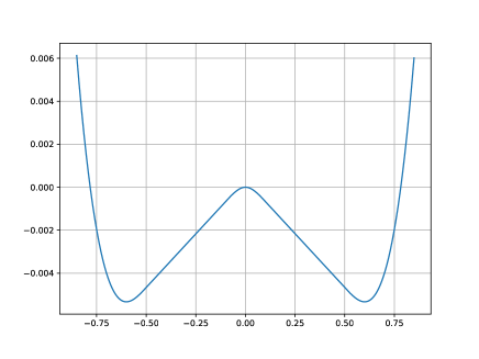
Figure 2: W-shape function designed by Tripuraneni et al. [47]

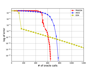
(a) Initial point $(x_{1},y_{1})$

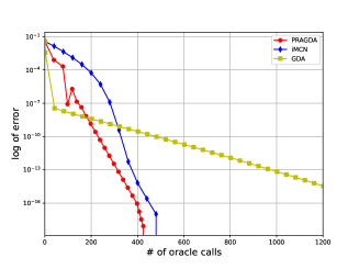
(b) Initial point $(x_{2},y_{2})$

Figure 3: Comparison of various minmax algorithms at different initial points

E.1 Synthetic Minimax Problem

We construct the following nonconvex-strong-concave minimax problem:

$$\min_{x\in\mathbb{R}^{3}}\max_{y\in\mathbb{R}^{2}}~{}f(x,y)=w(x_{3})-10y_{1}^{2}+x_{1}y_{1}-5y_{2}^{2}+x_{2}y_{2},$$

where $x=[x_{1},x_{2},x_{3}]^{T}$ and $y=[y_{1},y_{2}]^{T}$ and

$$w(x)=\left\{\begin{array}[]{ll}\sqrt{\epsilon}(x+(L+1)\sqrt{\epsilon}\,)^{2}-\frac{1}{3}(x+(L+1)\sqrt{\epsilon}\,)^{3}-\frac{1}{3}(3L+1)\epsilon^{3/2},&x\leq-L\sqrt{\epsilon};\\ \epsilon x+\frac{\epsilon^{3/2}}{3},&-L\sqrt{\epsilon}<x\leq-\sqrt{\epsilon};\\ -\sqrt{\epsilon}x^{2}-\frac{x^{3}}{3},&-\sqrt{\epsilon}<x\leq 0;\\ -\sqrt{\epsilon}x^{2}+\frac{x^{3}}{3},&0<x\leq\sqrt{\epsilon};\\ -\epsilon x+\frac{\epsilon^{3/2}}{3},&\sqrt{\epsilon}<x\leq L\sqrt{\epsilon};\\ \sqrt{\epsilon}(x-(L+1)\sqrt{\epsilon}\,)^{2}+\frac{1}{3}(x-(L+1)\sqrt{\epsilon}\,)^{3}-\frac{1}{3}(3L+1)\epsilon^{3/2},&L\sqrt{\epsilon}<x;\end{array}\right.$$

is the W-shape-function [47] and we set $\epsilon=0.01,L=5$ in our experiment. We visualize the $w(\cdot)$ in Figure 2. It is easy to verify that $(x_{0},y_{0})=([0,0,0]^{\top},[0,0]^{\top})$ is a saddle point of $f(x,y)$. We construct our experiment with two different initial points:

$$(x_{1},y_{1})=\left([10^{-3},10^{-3},10^{-16}]^{\top},[0,0]^{\top}\right)\qquad\text{and}\qquad(x_{2},y_{2})=\left([0,0,1]^{\top},[0,0]^{\top}\right).$$

Note that $(x_{1},y_{1})$ is close to $(x_{0},y_{0})$ while $(x_{2},y_{2})$ is far from $(x_{0},y_{0})$. We compare our PRAGDA with iMCN [38] algorithm and classical GDA [35] algorithm. The results are shown in Figure 3. We use a grid search to choose the learning rate of AGD steps and GDA and outer-loop learning rate of PRAGDA from $\{c\times 10^{i}:c\in\{1,5\},i\in\{1,2,3\}\}$ and the momentum parameter from $\{c\times 0.1:c\in\{1,2,3,4,5,6,7,8,9\}\}$.

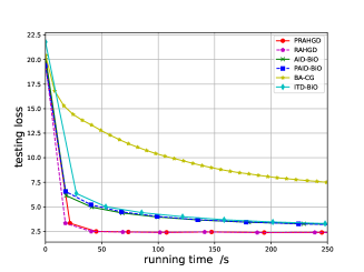
(a) Corruption rate p = 0.2

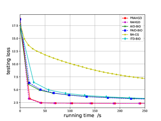
(b) Corruption rate p = 0.4

Figure 4: Comparison of various bilevel algorithms for data hypercleaning at different corruption rate

E.2 Data Hypercleaning

Data hypercleaning [15, 44] is a classic application of bilevel optimization. In practice, we may have a dataset with label noise and we could only offer some time or cost to cleanup a subset of the noise data. To train a model in such a setting, we can treat the cleaned data as the validation set and the rest data as the training set. Then it can be transferred into a bilevel optimization:

$$\min_{\lambda\in\mathbb{R}^{N_{\rm tr}}}f(W^{*}(\lambda),\lambda)\triangleq\frac{1}{|{\mathcal{D}}_{\rm val}|}\sum_{(x_{i},y_{i})\in{\mathcal{D}}_{\rm val}}-\log(y_{i}^{\top}W^{*}(\lambda)x_{i})$$ (42)

$$\textrm{s.t.}\quad W^{*}(\lambda)=\operatorname*{arg\,min}_{W\in\mathbb{R}^{d_{y}\times d_{x}}}\ g(W,\lambda)\triangleq\frac{1}{|{\mathcal{D}}_{\rm tr}|}\sum_{(x_{i},y_{i})\in{\mathcal{D}}_{\rm tr}}-\sigma(\lambda_{i})\log(y_{i}^{\top}Wx_{i})+C_{r}||W||^{2}\ ,$$

where ${\mathcal{D}}_{\rm tr}=\{(x_{i},y_{i})\}$ is the training dataset, ${\mathcal{D}}_{\rm val}=\{(x_{i},y_{i})\}$ is the validation dataset, $W$ is the weight of the classifier, $\lambda_{i}\in\mathbb{R}$, $\sigma$ is the sigmoid function and $C_{r}$ is a regularization parameter. Following Shaban et al. [44] and Ji et al. [25], we choose $C_{r}=0.001$.

We conducted the experiment on MNIST[31]. We have $x\in\mathbb{R}^{785}$, $y\in\mathbb{R}^{10}$ and $W\in\mathbb{R}^{10\times 785}$ in equation (42). Training set contains 20,000 images, some of which have their labels randomly disrupted. We called the ratio of images with disrupted labels as corruption rate $p$. Validation set contains 5,000 images with correct labels. The testing set consists 10,000 images. The results are shown in Figure 4.

For BA algorithm proposed by Ghadimi and Wang [17], we also use conjugate gradient descent method to compute the Hessian vector since they didn’t specify it and we called it BA-CG in Figure 4. For all algorithms, We choose the inner-loop learning rate and outer-loop learning rate from $\{0.001,0.01,0.1,1,10\}$ and the iteration number of CG step from $\{3,6,12,24\}$. For all algorithms except BA, we choose the iteration number of GD or AGD steps from $\{50,100,200,500,1000\}$ and for BA algorithm, as adopted by Ghadimi and Wang [17], we choose the iteration number of GD steps from $\{\lceil c(k+1)^{1/4}\rceil:c\in\{0.5,1,2,4\}\}$ . We observe that both RAHGD and PRAHGD converge faster than other algorithms.

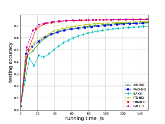
(a) testing accuracy vs. running time

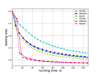
(b) testing lose vs. running time

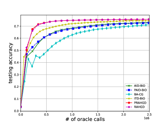
(c) testing accuracy vs. # of oracle calls

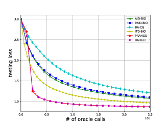
(d) testing lose vs. # of oracle calls

Figure 5: Comparison of various bilevel algorithms on logistic regression on 20 Newsgroup dataset. Figure (a) and (b) show the results of testing accuracy and testing lose vs.running time respectively. Figure (c) and (d) show the results of testing accuracy and testing lose vs. # of oracles calls respectively.

E.3 Hyperparemeter Optimization

Hyperparameter optimization is a classical bilevel problem. The goal of hyperparameter optimization is to find the optimal hyperparameter to minimize the loss on the validation dataset. We compare the performance of our algorithm RAHGD and PRAHGD with the baseline algorithms listed in Table 1 and Table 2 over a logistic regression problem on 20 News group dataset[20]. This dataset consists of 18,846 news items divided into 20 topics, and features include 130,170 tf-idf sparse vectors. We divided the data into three parts: 5,657 for training, 5,657 for validation, and 7,532 for testing. Then the objective function of this problem can be written in the following form.

$$\min_{\lambda\in\mathbb{R}^{p}}~{}\frac{1}{|{\mathcal{D}}_{\rm val}|}\sum_{(x_{i},y_{i})\in{\mathcal{D}}_{\rm val}}L(w^{*}(\lambda);x_{i},y_{i})$$

$$s.t.~{}\ w^{*}(\lambda)=\operatorname*{arg\,min}_{w\in\mathbb{R}^{c\times p}}\ \frac{1}{|{\mathcal{D}}_{\rm tr}|}\sum_{(x_{i},y_{i})\in{\mathcal{D}}_{\rm tr}}L(w;x_{i},y_{i})+\frac{1}{2cp}\sum_{j=1}^{c}\sum_{k=1}^{p}\exp(\lambda_{k})w_{jk}^{2},$$

where ${\mathcal{D}}_{\rm tr}=\{(x_{i},y_{i})\}$ is the training dataset, ${\mathcal{D}}_{\rm val}=\{(x_{i},y_{i})\}$ is the validation dataset, $L$ is the cross-entropy loss function, $c=20$ is the number of topics and $p=130,170$ is the dimension of features. Same as that in section E.2, we use the conjugate gradient descent method to approximate the Hessian vector.

For all algorithms listed in Figure 5, we choose the inner-loop learning rate and out-loop learning rate from $\{0.001,0.01,0.1,1,10,100,1000\}$, the iteration number of GD or AGD step from $\{5,10,30,50\}$, and the iteration number of CG step from $\{5,10,30,50\}$. For BA-CG, we choose the iteration number of GD steps from $\{\lceil c(k+1)^{1/4}\rceil:c\in\{0.5,1,2,4\}\}$ as adopted by Ghadimi and Wang [17]. The results are shown in Figure 5. We observe that our RAHGD and PRAHGD converge faster than other algorithms.

References

- Agarwal et al. [2017] Naman Agarwal, Zeyuan Allen-Zhu, Brian Bullins, Elad Hazan, and Tengyu Ma. Finding approximate local minima faster than gradient descent. In Proceedings of the 49th Annual ACM SIGACT Symposium on Theory of Computing, pages 1195–1199, 2017.
- Arjovsky et al. [2017] Martin Arjovsky, Soumith Chintala, and Léon Bottou. Wasserstein generative adversarial networks. In International Conference on Machine Learning, pages 214–223. PMLR, 2017.
- Bertinetto et al. [2018] Luca Bertinetto, Joao F. Henriques, Philip H.S. Torr, and Andrea Vedaldi. Meta-learning with differentiable closed-form solvers. arXiv preprint arXiv:1805.08136, 2018.
- Bhatia [1997] Rajendra Bhatia. Matrix Analysis, volume 169. Springer, 1997.
- Bracken and McGill [1973] Jerome Bracken and James T. McGill. Mathematical programs with optimization problems in the constraints. Operations Research, 21(1):37–44, 1973.
- Carmon et al. [2017] Yair Carmon, John C. Duchi, Oliver Hinder, and Aaron Sidford. Convex until proven guilty: Dimension-free acceleration of gradient descent on non-convex functions. In International Conference on Machine Learning, pages 654–663. PMLR, 2017.
- Carmon et al. [2018] Yair Carmon, John C. Duchi, Oliver Hinder, and Aaron Sidford. Accelerated methods for nonconvex optimization. SIAM Journal on Optimization, 28(2):1751–1772, 2018.
- Carmon et al. [2020] Yair Carmon, John C. Duchi, Oliver Hinder, and Aaron Sidford. Lower bounds for finding stationary points I. Mathematical Programming, 184(1):71–120, 2020.
- Chen et al. [2021a] Tianyi Chen, Yuejiao Sun, and Wotao Yin. Closing the gap: Tighter analysis of alternating stochastic gradient methods for bilevel problems. Advances in Neural Information Processing Systems, 34:25294–25307, 2021a.
- Chen et al. [2021b] Ziyi Chen, Qunwei Li, and Yi Zhou. Escaping saddle points in nonconvex minimax optimization via cubic-regularized gradient descent-ascent. arXiv preprint arXiv:2110.07098, 2021b.
- Curtis et al. [2017] Frank E. Curtis, Daniel P. Robinson, and Mohammadreza Samadi. A trust region algorithm with a worst-case iteration complexity of for nonconvex optimization. Mathematical Programming, 162:1–32, 2017.
- Dauphin et al. [2014] Yann N. Dauphin, Razvan Pascanu, Caglar Gulcehre, Kyunghyun Cho, Surya Ganguli, and Yoshua Bengio. Identifying and attacking the saddle point problem in high-dimensional non-convex optimization. Advances in Neural Information Processing Systems, 27, 2014.
- Feurer and Hutter [2019] Matthias Feurer and Frank Hutter. Hyperparameter optimization. In Automated Machine Learning, pages 3–33. Springer, Cham, 2019.
- Fiez et al. [2021] Tanner Fiez, Lillian Ratliff, Eric Mazumdar, Evan Faulkner, and Adhyyan Narang. Global convergence to local minmax equilibrium in classes of nonconvex zero-sum games. Advances in Neural Information Processing Systems, 34:29049–29063, 2021.
- Franceschi et al. [2017] Luca Franceschi, Michele Donini, Paolo Frasconi, and Massimiliano Pontil. Forward and reverse gradient-based hyperparameter optimization. In International Conference on Machine Learning, pages 1165–1173. PMLR, 2017.
- Franceschi et al. [2018] Luca Franceschi, Paolo Frasconi, Saverio Salzo, Riccardo Grazzi, and Massimiliano Pontil. Bilevel programming for hyperparameter optimization and meta-learning. In International Conference on Machine Learning, pages 1568–1577. PMLR, 2018.
- Ghadimi and Wang [2018] Saeed Ghadimi and Mengdi Wang. Approximation methods for bilevel programming. arXiv preprint arXiv:1802.02246, 2018.
- Goodfellow et al. [2020] Ian Goodfellow, Jean Pouget-Abadie, Mehdi Mirza, Bing Xu, David Warde-Farley, Sherjil Ozair, Aaron Courville, and Yoshua Bengio. Generative adversarial networks. Communications of the ACM, 63(11):139–144, 2020.
- Goodfellow et al. [2014] Ian J. Goodfellow, Jonathon Shlens, and Christian Szegedy. Explaining and harnessing adversarial examples. arXiv preprint arXiv:1412.6572, 2014.
- Grazzi et al. [2020] Riccardo Grazzi, Luca Franceschi, Massimiliano Pontil, and Saverio Salzo. On the iteration complexity of hypergradient computation. In International Conference on Machine Learning, pages 3748–3758. PMLR, 2020.
- Hong et al. [2020] Mingyi Hong, Hoi-To Wai, Zhaoran Wang, and Zhuoran Yang. A two-timescale framework for bilevel optimization: Complexity analysis and application to actor-critic. arXiv preprint arXiv:2007.05170, 2020.
- Huang et al. [2021] Minhui Huang, Shiqian Ma, and Lifeng Lai. A Riemannian block coordinate descent method for computing the projection robust wasserstein distance. In International Conference on Machine Learning, pages 4446–4455. PMLR, 2021.
- Huang et al. [2022] Minhui Huang, Kaiyi Ji, Shiqian Ma, and Lifeng Lai. Efficiently escaping saddle points in bilevel optimization. arXiv preprint arXiv:2202.03684, 2022.
- Ji et al. [2020] Kaiyi Ji, Jason D. Lee, Yingbin Liang, and H. Vincent Poor. Convergence of meta-learning with task-specific adaptation over partial parameters. Advances in Neural Information Processing Systems, 33:11490–11500, 2020.
- Ji et al. [2021] Kaiyi Ji, Junjie Yang, and Yingbin Liang. Bilevel optimization: Convergence analysis and enhanced design. In International Conference on Machine Learning, pages 4882–4892. PMLR, 2021.
- Ji et al. [2022] Kaiyi Ji, Mingrui Liu, Yingbin Liang, and Lei Ying. Will bilevel optimizers benefit from loops. arXiv preprint arXiv:2205.14224, 2022.
- Jin et al. [2017] Chi Jin, Rong Ge, Praneeth Netrapalli, Sham M. Kakade, and Michael I. Jordan. How to escape saddle points efficiently. In International conference on machine learning, pages 1724–1732. PMLR, 2017.
- Jin et al. [2018] Chi Jin, Praneeth Netrapalli, and Michael I. Jordan. Accelerated gradient descent escapes saddle points faster than gradient descent. In Conference On Learning Theory, pages 1042–1085. PMLR, 2018.
- Jin et al. [2020] Chi Jin, Praneeth Netrapalli, and Michael I. Jordan. What is local optimality in nonconvex-nonconcave minimax optimization? In International Conference on Machine Learning, pages 4880–4889. PMLR, 2020.
- Konda and Tsitsiklis [1999] Vijay Konda and John Tsitsiklis. Actor-critic algorithms. Advances in Neural Information Processing Systems, 12, 1999.
- LeCun et al. [1998] Yann LeCun, Léon Bottou, Yoshua Bengio, and Patrick Haffner. Gradient-based learning applied to document recognition. Proceedings of the IEEE, 86(11):2278–2324, 1998.
- Lee et al. [2019] Jason D. Lee, Ioannis Panageas, Georgios Piliouras, Max Simchowitz, Michael I. Jordan, and Benjamin Recht. First-order methods almost always avoid strict saddle points. Mathematical Programming, 176:311–337, 2019.
- Li and Lin [2022] Huan Li and Zhouchen Lin. Restarted nonconvex accelerated gradient descent: No more polylogarithmic factor in the complexity. In International Conference on Machine Learning, pages 12901–12916. PMLR, 2022.
- Lin et al. [2020a] Tianyi Lin, Chenyou Fan, Nhat Ho, Marco Cuturi, and Michael I. Jordan. Projection robust Wasserstein distance and Riemannian optimization. Advances in Neural Information Processing Systems, 33:9383–9397, 2020a.
- Lin et al. [2020b] Tianyi Lin, Chi Jin, and Michael I. Jordan. On gradient descent ascent for nonconvex-concave minimax problems. In International Conference on Machine Learning, pages 6083–6093. PMLR, 2020b.
- Lu et al. [2020] Songtao Lu, Ioannis Tsaknakis, Mingyi Hong, and Yongxin Chen. Hybrid block successive approximation for one-sided non-convex min-max problems: algorithms and applications. IEEE Transactions on Signal Processing, 68:3676–3691, 2020.
- Luo et al. [2020] Luo Luo, Haishan Ye, Zhichao Huang, and Tong Zhang. Stochastic recursive gradient descent ascent for stochastic nonconvex-strongly-concave minimax problems. Advances in Neural Information Processing Systems, 33:20566–20577, 2020.
- Luo et al. [2022] Luo Luo, Yujun Li, and Cheng Chen. Finding second-order stationary points in nonconvex-strongly-concave minimax optimization. In Advances in Neural Information Processing Systems, 2022.
- Nesterov [2013] Yurii Nesterov. Introductory Lectures on Convex Optimization: A Basic Course, volume 87. Springer Science & Business Media, 2013.
- Nesterov and Polyak [2006] Yurii Nesterov and Boris T. Polyak. Cubic regularization of Newton method and its global performance. Mathematical Programming, 108(1):177–205, 2006.
- Nocedal and Wright [2006] Jorge Nocedal and Stephen J. Wright. Numerical Optimization. Springer, 2nd edition, 2006.
- Nouiehed et al. [2019] Maher Nouiehed, Maziar Sanjabi, Tianjian Huang, Jason D. Lee, and Meisam Razaviyayn. Solving a class of non-convex min-max games using iterative first order methods. Advances in Neural Information Processing Systems, 32, 2019.
- Rudin [1976] Walter Rudin. Principles of Mathematical Analysis. McGraw-Hill, New York, 1976.
- Shaban et al. [2019] Amirreza Shaban, Ching-An Cheng, Nathan Hatch, and Byron Boots. Truncated back-propagation for bilevel optimization. In The 22nd International Conference on Artificial Intelligence and Statistics, pages 1723–1732. PMLR, 2019.
- Sinha et al. [2018] Aman Sinha, Hongseok Namkoong, Riccardo Volpi, and John Duchi. Certifying some distributional robustness with principled adversarial training. In International Conference on Learning Representations, 2018.
- Stadie et al. [2020] Bradly Stadie, Lunjun Zhang, and Jimmy Ba. Learning intrinsic rewards as a bi-level optimization problem. In Conference on Uncertainty in Artificial Intelligence, pages 111–120. PMLR, 2020.
- Tripuraneni et al. [2018] Nilesh Tripuraneni, Mitchell Stern, Chi Jin, Jeffrey Regier, and Michael I. Jordan. Stochastic cubic regularization for fast nonconvex optimization. Advances in Neural Information Processing Systems, 31, 2018.
- Zhang et al. [2020] Jiawei Zhang, Peijun Xiao, Ruoyu Sun, and Zhi-Quan Luo. A single-loop smoothed gradient descent-ascent algorithm for nonconvex-concave min-max problems. Advances in Neural Information Processing Systems, 33:7377–7389, 2020.