Isotope effects in the electronic spectra of ammonia from ab initio semiclassical dynamics

Abstract

Despite its simplicity, the single-trajectory thawed Gaussian approximation has proven useful for calculating vibrationally resolved electronic spectra of molecules with weakly anharmonic potential energy surfaces. Here, we show that the thawed Gaussian approximation can capture surprisingly well even more subtle observables, such as the isotope effects in the absorption spectra, and we demonstrate it on the four isotopologues of ammonia (NH₃, NDH₂, ND₂H, ND₃). The differences in their computed spectra are due to the differences in the semiclassical trajectories followed by the four isotopologues, and the isotope effects—narrowing of the transition band and reduction of the peak spacing—are accurately described by this semiclassical method. In contrast, the adiabatic harmonic model shows a double progression instead of the single progression seen in the experimental spectra. The vertical harmonic model correctly shows only a single progression but fails to describe the anharmonic peak spacing. Analysis of the normal-mode activation upon excitation provides insight into the elusiveness of the symmetric stretching progression in the spectra.

EPFL]Laboratory of Theoretical Physical Chemistry, Institut des Sciences et Ingénierie Chimiques, Ecole Polytechnique Fédérale de Lausanne (EPFL), CH-1015, Lausanne, Switzerland EPFL]Laboratory of Theoretical Physical Chemistry, Institut des Sciences et Ingénierie Chimiques, Ecole Polytechnique Fédérale de Lausanne (EPFL), CH-1015, Lausanne, Switzerland

Vibrationally resolved electronic spectroscopy has made significant contributions to the understanding of the structure and dynamics of molecules. However, extracting information about the potential energy surface (PES) on which the dynamics occur remains challenging due to several factors influencing the experimentally observed spectra. Since the electronic structure is invariant to the isotope substitution, measuring the isotope effects in the spectra not only provides additional information about the shape of the surface and dynamics, but also aids in the assignment of transitions. Computational methods help to interpret experimental results and provide a clearer understanding of the dynamics responsible for the observed spectra.

Within the Born-Oppenheimer approximation,^{1, 2} the isotope effects in the spectra are attributed to the changes in the characteristic frequencies of isotopologues, which depend strongly on the mass of the substituted atom. Depending on the system of interest, the isotope exchange can shift the peak positions to higher or lower energies. In general, the isotope substitution changes the energy of the 0-0 transition, the width of the transition band, and also the spacing, widths, and intensities of peaks. The magnitude of these changes depends on the mass ratio of the substituted species and on the displacement in the vibrational normal modes responsible for the spectra.^{3, 4}

Among the various methods for calculating the isotope effects in the spectra, the simplest approach is based on the global harmonic approximation to the potential.^{5, 6, 7, 8, 9} Harmonic models are computationally cheap and can capture some isotope effects correctly but fail in systems with a large-amplitude nuclear motion.¹⁰ In contrast, the exact quantum dynamics on a grid¹¹ or multiconfigurational time-dependent Hartree (MCTDH) method¹² reproduce all of the isotope effects seen in the experimental spectra, but at the high cost of constructing a global PES.¹³ A compromise is offered by the semiclassical trajectory-based methods, which, in terms of accuracy, lie between the harmonic and exact results.^{14, 15, 16, 17, 18, 19, 20, 21, 22, 23, 24, 25, 26}

The single-trajectory thawed Gaussian approximation (TGA), introduced by Heller,²⁷ is a semiclassical method, which is accurate for short propagation times and which has been used to calculate both absorption and emission spectra of weakly anharmonic molecules with a large number of degrees of freedom.^{28, 15, 16} In weakly anharmonic systems and for short times relevant in electronic spectroscopy, the single Gaussian wavepacket used in the TGA is, sometimes surprisingly, sufficient to sample the dynamically important region of the phase space. Moreover, the classical trajectory associated with the wavefunction provides a simplified, intuitive picture of the dynamics, while the evolving width of the Gaussian wavepacket partially captures the quantum effects. Successful past applications of the TGA prompted us to apply it to the isotope effects. Although the PES used for the propagation is invariant under the isotope substitution, for each isotopologue, the guiding trajectory explores a different region of this common PES. This requires propagating a new trajectory for each isotopologue, but the total computational cost is still considerably lower than the cost of constructing the full surface.

To investigate the isotope effect on the spectrum, a comprehensive understanding of the PES associated with the transition is essential. In the case of ammonia, the first excited-state $\tilde{A}$ is quasi-bound in the Franck-Condon region.^{29, 30} A finite barrier separates the bound region from the conical intersection of the $\tilde{X}$ and $\tilde{A}$ states. This conical intersection couples the two surfaces nonadiabatically and is responsible for an internal conversion, which leads to the broadening of the absorption spectra.^{31, 32, 33} The lifetime in the quasi-bound region depends on the isotopologue and ranges from a few hundred femtoseconds to a few picoseconds, allowing for more than several oscillations to occur before the escape. The ammonia absorption spectra $\tilde{A}^{1}A_{2}^{\prime\prime}\longleftarrow\tilde{X}^{1}A_{1}^{\prime}$ ($S_{1}\longleftarrow S_{0}$) has a long progression that is induced by the activation of the symmetric bending (umbrella motion) and symmetric stretching modes.^{34, 35, 36} Although the experimental spectra of isotopologues (NDH₂, ND₂H, ND₃) have similar patterns as the spectrum of NH₃, the isotope effects are clearly visible.³⁷ As the number of hydrogen atoms substituted by deuterium increases, the energy of the 0-0 transition increases, while the peak spacing and width decreases. In addition, the transition band becomes narrower.

The isotope substitution can also affect the molecular symmetry. Although the ground-state geometry of all four ammonia isotopologues has a pyramidal shape, the NH₃ and ND₃ belong to the C_3v point group, whereas NDH₂ and ND₂H belong to the C_s point group. As the symmetry changes from one isotopologue to another, the dynamics on the excited-state surface changes not only due to the change of reduced masses, but also due to the activation of other normal modes.⁴

To demonstrate various isotope effects on electronic spectra, let us first consider an analytically solvable one-dimensional displaced harmonic oscillator model. In this model, the two PESs involved in the transition are described by harmonic oscillators with the same force constant ($k_{g}=k_{e}=k$), but whose minima are displaced horizontally by $\Delta q$ and vertically by an energy gap $\Delta E$. Assuming that the initial state is the vibrational ground state $|\Psi_{g,0}\rangle$ of the electronic ground state, the Franck-Condon factors, which determine the transition probability between two vibronic states and hence the intensities of the spectral peaks, follow the Poisson distribution

$$|\langle\Psi_{g,0}|\Psi_{e,n}\rangle|^{2}=e^{-S_{ge}}\frac{S_{ge}^{n}}{n!},$$ (1)

where $S_{ge}=\Delta q^{2}\frac{\mu\omega_{g}}{2\hbar}$ is the Huang-Rhys parameter for the ground and excited states, $\omega_{g}=(k_{g}/\mu)^{1/2}$, and $\mu$ is the reduced mass of the oscillator. Analytical expressions for Franck-Condon factors for squeezed and displaced harmonic oscillators (in which $k_{e}\neq k_{g}$) can be found, e.g., in Ref. 38. The spectra computed in these model systems with the time-independent approach are compared with the results obtained with the TGA, which is exact in quadratic potentials, in Fig. 1. In spite of the simplicity of the models, the spectra exhibit all of the above-mentioned isotope effects—namely the changes in the 0-0 transition, peak spacing, width of the transition band—except for the effect on the peak widths, which is zero in the time-independent approach and arbitrary in the TGA (due to the choice of the damping of the wavepacket time autocorrelation function). Note that the 0-0 transition is only affected in the distorted model, where the vibrational frequencies of the ground and excited states differ.

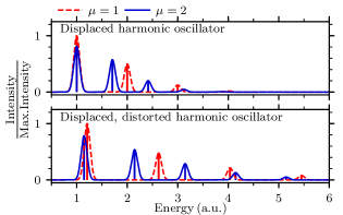
Figure 1: Isotope effects in the electronic spectra of one-dimensional harmonic oscillators. The finite-width peaks were obtained with the TGA, whereas the vertical lines indicate the spectra obtained with the time-independent approach,^{39, 40} in which the Franck-Condon factors were calculated with Eq. (1) (in the top panel) or Eq. (3.26) from Ref. 38 (in the bottom panel). The spectra were scaled according to the maximum intensity of the system with $\mu=1$. The details of this calculation can be found in the Supporting Information.

Polyatomic molecules with at least two vibrational degrees of freedom pose an additional challenge due to the multidimensional nature of their potential energy surfaces. Within the harmonic approximation, the excited-state potential energy surface $V(q)$ of a molecule is approximated by a quadratic expansion about the reference geometry $q_{\text{ref}}$:

$$V_{\text{HA}}(q)=V|_{q_{\text{ref}}}+V^{\prime}|_{q_{\text{ref}}}^{T}\cdot x_{r}+x_{r}^{T}\cdot V^{\prime\prime}|_{q_{\text{ref}}}\cdot x_{r}/2,$$ (2)

where $x_{r}:=q-q_{\text{ref}}$, $V^{\prime}|_{q_{\text{ref}}}=\text{grad}_{q}V|_{q_{\text{ref}}}$ is the gradient vector, and $V^{\prime\prime}|_{q_{\text{ref}}}=\text{Hess}_{q}V|_{q_{\text{ref}}}$ is the Hessian matrix at the reference geometry. The PES of the excited state is generally not only displaced and distorted but also rotated with respect to the surface of the initial state. This rotation is called the Duschinsky effect and is characterized by the Duschinsky matrix $J$ that relates the normal-mode coordinates of the two states.⁴¹ The general form of the potential in Eq. (2) allows for a free choice of $q_{\text{ref}}$, but two choices are the most natural. The adiabatic harmonic model is constructed about the equilibrium geometry of the excited-state surface, whereas the vertical harmonic model expands the excited-state surface about the Franck-Condon geometry, i.e., the equilibrium geometry of the ground-state surface.^{6, 42} Various exact and efficient algorithms are able to treat global harmonic models of large systems, and the thawed Gaussian approximation is one of them. The harmonic models are easy to construct, as they only require a single Hessian calculation in the ground and excited states once the geometries have been optimized. The subsequent evaluation of the autocorrelation functions and spectra requires much less computational effort. The drawback of the harmonic models is the complete neglect of anharmonicity, which may lead to erroneous results for systems with a large amplitude nuclear motion.

Going beyond the harmonic approximation requires the inclusion of anharmonicity effects, and Heller’s²⁷ thawed Gaussian approximation does it at least partially by employing the local harmonic approximation

$$V_{\text{LHA}}(q;q_{t})= V|_{q_{t}}+V^{\prime}|_{q_{t}}^{T}\cdot x_{t}$$

$$+x_{t}^{T}\cdot V^{\prime\prime}|_{q_{t}}\cdot x_{t}/2$$ (3)

of the potential about the current center $q_{t}$ of the wavepacket ($x_{t}:=q-q_{t}$). The TGA allows the exploration of anharmonic parts of the potential without the need to construct a full PES a priori. Within the time-dependent approach to spectroscopy,^{43, 39} the nuclear wavepacket is propagated by solving the time-dependent Schrödinger equation

$$i\hbar|\dot{\Psi}_{t}\rangle=\hat{H}|\Psi_{t}\rangle,$$ (4)

where $|\Psi_{t}\rangle$ is the nuclear wavepacket, $\hat{H}:=\hat{p}^{T}\cdot m^{-1}\cdot\hat{p}/2+V(\hat{q})$ is the vibrational Hamiltonian, and  $m=\text{diag}(m_{1},...,m_{D})$ is the diagonal mass-matrix. The thawed Gaussian approximation assumes that the nuclear wavepacket is a $D$-dimensional Gaussian,^{44, 45} which, in Hagedorn’s parametrization,^{46, 47} is written as

$$\psi(q,t)=N_{t}\exp\Big{[}\frac{i}{\hbar}\Big{(} \frac{1}{2}x_{t}^{T}\cdot P_{t}\cdot Q_{t}^{-1}\cdot x_{t}$$

$$+p_{t}^{T}\cdot x_{t}+S_{t}\Big{)}\Big{]},$$ (5)

where $N_{t}=(\pi\hbar)^{-D/4}(\text{det}Q_{t})^{-1/2}$ is the normalization constant, $x_{t}:=q-q_{t}$ is the shifted position, $q_{t}$ and $p_{t}$ are the position and momentum of the wavepacket’s center, $S_{t}$ is the classical action, and $P_{t}$, $Q_{t}$ are complex $D\times D$ matrices, which satisfy the relations

$$Q_{t}^{T}\cdot P_{t}-P_{t}\cdot Q_{t} =0,$$ (6)

$$Q_{t}^{\dagger}\cdot P_{t}-P_{t}^{\dagger}\cdot Q_{t} =2iI_{D},$$ (7)

in which $I_{D}$ is the $D\times D$ identity matrix. Approximating $V$ with $V_{\text{LHA}}$ in the Schrödinger Eq. (4) yields the nonlinear Schrödinger equation

$$i\hbar|\dot{\Psi}_{t}\rangle=[\hat{p}^{T}\cdot m^{-1}\cdot\hat{p}/2+V(\hat{q};q_{t})]|\Psi_{t}\rangle.$$

This equation is solved exactly by the Gaussian ansatz if the Gaussian’s parameters satisfy the first-order differential equations

$$\dot{q}_{t} =m^{-1}\cdot p_{t},$$ (8)

$$\dot{p}_{t} =-\text{grad}_{q}V|_{q^{t}},$$ (9)

$$\dot{Q}_{t} =m^{-1}\cdot P_{t},$$ (10)

$$\dot{P}_{t} =-\text{Hess}_{q}V|_{q^{t}}\cdot Q_{t},$$ (11)

$$\dot{S}_{t} =L_{t},$$ (12)

where $L_{t}$ denotes the Lagrangian

$$L_{t} =\dot{q}_{t}^{T}\cdot m\cdot\dot{q}_{t}/2-V(q_{t})$$

$$=p_{t}^{T}\cdot m^{-1}\cdot p_{t}/2-V(q_{t}).$$ (13)

Equations (8) and (9) imply that the center of the wavepacket follows exactly the classical trajectory of the original potential, while the width of the Gaussian is propagated with the effective potential $V_{\text{LHA}}(q_{t})$ [see Eqs. (10) and (11)].

Being a single-trajectory method, the TGA can be easily combined with an on-the-fly evaluation of the electronic structure. Most often, electronic structure calculations for a molecule with $N$ atoms are performed in $3N$ Cartesian coordinates. However, natural coordinates for the propagation of the thawed Gaussian wavepacket and for the construction of global harmonic models are the $3N-6$ mass-scaled vibrational normal-mode coordinates $q_{j}$. We perform the propagation in the excited-state vibrational normal-mode coordinates, since these coordinates provide the most natural description of the dynamics following the electronic excitation. The transformation from the Cartesian to normal-mode coordinates requires the removal of translational and rotational degrees of freedom. Although the vibrations and rotations are not fully separable, we reduce the coupling by translating and rotating the nuclei of the molecule into the Eckart frame. Here, we closely follow the procedure described in more detail in Ref. 43.

Let us denote the full molecular configuration as $\xi:=(\mathbf{r}_{1},\dots,\mathbf{r}_{N})$, where $\mathbf{r}_{a}$ are the Cartesian coordinates of atom $a$. We introduce a reference molecular configuration $\xi_{\text{ref}}:=(\mathbf{r}_{\text{ref},1},\dots,\mathbf{r}_{\text{ref},N})$. In all our calculations $\xi_{\text{ref}}$ is the equilibrium geometry on the PES of the excited state $\tilde{A}$ of ammonia. First, the translational degrees of freedom are removed by shifting coordinates of each atom to the center-of-mass frame:

$$\mathbf{r}_{a}^{\prime}:=\mathbf{r}_{a}-\mathbf{r}_{\text{com}},$$ (14)

where $\mathbf{r}_{\text{com}}=(\sum_{a=1}^{N}m_{a}\mathbf{r}_{a})/(\sum_{a=1}^{N}m_{a})$ and $m_{a}$ is the mass of the nucleus of atom $a$. The translated molecular configuration is $\xi^{\prime}:=(\mathbf{r}^{\prime}_{1},\dots,\mathbf{r}^{\prime}_{N})$. In the following, we assume that the center of mass of the reference configuration $\xi_{\text{ref}}$ is at the origin, i.e., $\mathbf{r}_{\text{ref,com}}=0$.

In the second step, we minimize the rovibrational coupling by rotating the configuration $\xi^{\prime}$ into the Eckart frame. This is equivalent to minimizing the squared mass-scaled distance⁴⁸

$$||\xi_{\text{ref}}-\xi_{\text{rot}}||^{2}:=\sum_{a=1}^{N}m_{a}|\mathbf{r}_{\text{ref,a}}-\mathbf{r}_{\text{rot,a}}|^{2},$$ (15)

between the rotated configuration $\xi_{\text{rot}}$ and the reference configuration $\xi_{\text{ref}}$. Here $\mathbf{r}_{\text{rot,a}}:=R\cdot\mathbf{r}^{\prime}_{a}$. The required $3\times 3$ rotation matrix $R$ can be found, e.g., by the Kabsch algorithm.⁴⁹ The transformation to and from normal-mode coordinates is based on the orthogonal matrix $O_{\text{ref}}$ that diagonalizes the mass-scaled Cartesian Hessian matrix at $\xi_{\text{ref}}$ on the excited-state surface $V$:

$$O_{\text{ref}}^{T}\cdot m^{-1/2}\cdot\text{Hess}_{\xi}V|_{\xi_{\text{ref}}}\cdot m^{-1/2}\cdot O_{\text{ref}}=\Omega^{2},$$ (16)

where $m$ and $\Omega$ are $3N\times 3N$ diagonal matrices, containing, respectively the values of the atomic masses and normal-mode frequencies (still including the zero frequencies). After projecting out the zero-frequency modes associated with rotations and translations, the overall transformation from the Cartesian coordinates $\xi$ to the mass-scaled vibrational normal-mode coordinates $q$ is

$$q=L_{\text{ref}}^{T}\cdot m^{\frac{1}{2}}\cdot(R_{\xi}\cdot\xi^{\prime}-\xi_{\text{ref}}),$$ (17)

where $L_{\text{ref}}$ is the leading $3N\times(3N-6)$ submatrix of $O_{\text{ref}}$, and $R_{\xi}=I_{N}\otimes R$ is a $3N\times 3N$ block-diagonal matrix, whose $N$ $3\times 3$ blocks are identical and equal to the rotation matrix $R$. Similarly, we can obtain the potential gradient and Hessian in vibrational normal-mode coordinates:

$$\text{grad}_{q}V =L_{\text{ref}}^{T}\cdot m^{-\frac{1}{2}}\cdot R_{\xi}\cdot\text{grad}_{\xi},$$ (18)

$$\text{Hess}_{q}V =L_{\text{ref}}^{T}\cdot m^{-\frac{1}{2}}\cdot R_{\xi}\cdot\text{Hess}_{\xi}\cdot R_{\xi}^{T}\cdot m^{-\frac{1}{2}}\cdot L_{\text{ref}}.$$ (19)

Equation (17) can be rearranged to transform the normal-mode coordinates back to the Cartesian coordinates as

$$\xi_{\text{rot}}=m^{\text{-}\frac{1}{2}}\cdot L_{\text{ref}}\cdot q+\xi_{\text{ref}}.$$ (20)

The above framework allows combining ab initio calculations in Cartesian coordinates with the propagation of the thawed Gaussian wavepacket in normal-mode coordinates. Equations (17)–(19) are also used for the construction of global harmonic models.

In what follows, all ab initio calculations of ammonia were performed using the complete active-space second-order perturbation theory CASPT2(8/8) method with Dunnings correlation-consistent basis set aug-cc-pVTZ; a level shift of 0.2 a.u. was applied to avoid the intruder-state problem. ^{50, 51} All of the calculations were performed with Molpro2019 package.⁵² The Gaussian wavepacket was propagated with a time step of 8 a.u. for 1000 steps (1 a.u. $\approx$ 0.024 fs resulting in a total time of 8000 a.u. $\approx 193.5$ fs) using the second-order symplectic integrator.⁵³ To remove the systematic errors of the ab initio vertical excitation energies, all computed spectra in Fig. 2 were shifted independently to obtain the best fit to the experiment. In addition, the spectra were broadened by a Lorentzian with half-width-at-half-maximum of 170, 137, 95, and 110 cm^-1 for NH₃, NDH₂, ND₂H, and ND₃, respectively. Neither the overall shift nor the broadening affect the subsequent analysis of peak spacing, peak intensities, and width of the spectral envelope, which are independent of the shift and broadening. Additional details can be found in the Supporting Information.

The initial Gaussian wavepacket was the ground vibrational eigenstate of the harmonic fit to the PES of the ground electronic state ($\tilde{X}^{1}A_{1}^{\prime}$) at one of the two degenerate minima. The initial position $q_{0}$ in normal-mode coordinates was obtained from Eq. (17), where $\xi^{\prime}$ is replaced with the Cartesian coordinates $\xi_{\text{init}}$ corresponding to the equilibrium geometry of the ground state. The initial momentum $p_{0}$ of the wavepacket was zero. The initial $Q_{0}$ and $P_{0}$ matrices, which control the width of the Gaussian wavepacket, were

$$P_{0}=i\hbar\Gamma^{\frac{1}{2}}\quad\text{and}\quad Q_{0}=\hbar\Gamma^{-\frac{1}{2}},$$ (21)

where $\Gamma:=\text{Hess}_{q}V^{(g)}|_{q_{0}}$ is the Hessian in normal-mode coordinates calculated at the equilibrium geometry of the ground state.

The experimental spectra of ammonia isotopologues, shown in the top left-hand panel of Fig. 2, clearly exhibit the isotope effects on the 0-0 transition energy, on the width of the transition band, and on the peak spacing, width, and intensity. First, the shift in the 0-0 transition towards higher energies can be directly compared with the adiabatic excitation energy from ab initio calculations in Table 1, indicating that quantum chemical calculations correctly reproduce the trend. Second, the bands associated to the $\tilde{A}^{1}A_{2}^{\prime\prime}\longleftarrow\tilde{X}^{1}A_{1}^{\prime}$ transition become narrower. Third, the decrease in the peak spacing for highly substituted species is in line with the fact that the spacing between the vibrational energy levels decreases with increasing reduced mass. Lastly, the nonradiative processes, such as tunnelling and internal conversion,³³ may cause the increase in the peak widths. Indeed, highly deuterated isotopologues have spectra with narrower peaks because they have a longer lifetime in the quasi-bound region, which is due to the weaker tunneling for heavier isotopes.

	NDH2	ND2H	ND3
Experiment	171	347	532
Adiabatic excitation energy	128	260	399

Table 1: Isotope effect on the 0-0 transition of ammonia evaluated as the difference $\Delta E_{00}(\text{ND}_{j}\text{H}_{i})-\Delta E_{00}(\text{NH}_{3})$. The adiabatic excitation energy includes the zero-point vibrational energy. All values shown are in cm^-1.

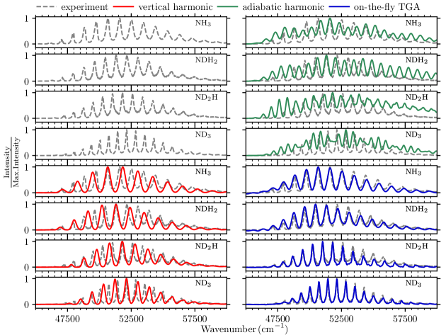
Figure 2: Simulated electronic absorption spectra of ammonia isotopologues (NH₃, NDH₂, ND₂H, and ND₃) are compared to the experimental spectra³⁷ recorded in the gas phase at 298 K.

The adiabatic harmonic model is constructed around the excited-state equilibrium geometry, and the same Cartesian Hessian is used to construct the PES for all isotopologues. The calculated spectra in the top right-hand panel of Fig. 2 show a double progression. In addition, for all isotopologues the spectral envelope extends to higher energies, reflecting the poor description of the short-time dynamics of the system. Overall, this confirms that the adiabatic harmonic model is a bad approximation of the strongly anharmonic PES of the ammonia molecule, where the differences between ground- and excited-state equilibrium geometries are significant. In the following, we do not discuss the isotope effect on the 0-0 transition, since the shift applied to compensate for the overall errors of the electronic structure calculations (see Supporting Information) is of the same order as the expected isotope effect. Instead, we focus on the isotope effects that are independent of this shift.

As observed in Ref. 16, the vertical harmonic model in the case of NH₃ yields a single progression and recovers the overall shape of the experimental spectrum. The results for other isotopologues further confirm this observation. Moreover, the computed envelopes of the spectra of all isotopologues agree rather well with the envelopes of the experimental spectra. This is because the vertical harmonic model approximates the PES well in the Franck-Condon region, which determines the spectral envelope. The widths of spectral envelopes are predicted rather accurately (see Table 2). The model also describes qualitatively the trend of decreasing peak spacing. However, as the model fails to capture anharmonicity, the peak spacing is not reproduced quantitatively.

	NH3	NDH2	ND2H	ND3
Exp.	5554	5030	4700	4638
TGA	5426	5342	4792	4558
vertical harmonic	5466	5202	4808	4490
adiabatic harmonic	7044	7224	5540	5748

Table 2: Width of the spectral envelope in cm^-1. The width of the spectral envelope was estimated as twice the square root of the weighted variance of the peak positions, where the weight of a peak position is given by its intensity (see the Supporting Information for details).

Within the thawed Gaussian approximation, the classical trajectory guiding the center of the wavepacket follows the exact and fully anharmonic ab initio PES, whereas the width of the wavepacket feels anharmonicity only approximately through the effective, locally harmonic potential. This on-the-fly approach improves over both global harmonic models and recovers well the isotope effects on the peak spacing and width of the spectral envelope. The intensities of the peaks are reproduced very well near the 0-0 transition, whereas the differences are more pronounced at higher energies for all isotopologues. The isotope effect on the peak spacing in Fig. 3 shows a remarkable agreement with the experiment with slight differences only near the 0-0 transition. In contrast, both harmonic models deviate substantially from the linear dependency of the shift on the peak frequency. The better performance of the on-the-fly TGA suggests that the fully anharmonic classical trajectory employed in the TGA describes better the true periodicity of the oscillations in the quasi-bound region of the $\tilde{A}$ state. Although a new calculation must be performed for each isotopologue, the results clearly indicate that this pays off.

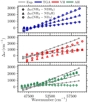
Figure 3: Isotope effects on the peak spacing in the $\tilde{A}^{1}A_{2}^{\prime\prime}\longleftarrow\tilde{X}^{1}A_{1}^{\prime}$ band computed with the on-the-fly thawed Gaussian approximation (TGA), adiabatic harmonic (AH) model, and vertical harmonic (VH) model are compared with the experimental values. $\Delta\omega$ is the difference between the wavenumbers of corresponding peaks in the spectra of two isotopologues.

One of the strengths of semiclassical methods is the ease with which they reveal the molecular dynamics that generate these spectra. The thawed Gaussian approximation makes this interpretation even simpler because it relies on only one trajectory. Having performed all the calculations in the excited-state normal-mode coordinates (depicted in Fig. 4), we also know the time evolution of each of these modes. In ammonia, the majority of the excited-state normal modes are similar to the more commonly used ground-state normal modes. In the case of NH₃ and ND₃, where the excited-state equilibrium geometry belongs to the D_3h point group, there are two pairs of degenerate normal modes—a degenerate pair of asymmetric stretching modes and a degenerate pair of scissoring modes. The other two modes—symmetric stretching and symmetric bending (umbrella motion)— are nondegenerate. In the case of partially deuterated isotopologues (NDH₂ and ND₂H), where the symmetry of the excited-state equilibrium geometry belongs to the C_2v point group, all six normal modes are nondegenerate.

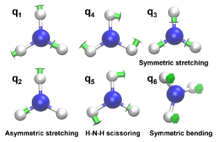
Figure 4: Vibrational normal modes of the excited electronic state of ammonia. In NH₃ and ND₃ the two asymmetric stretching modes ($q_{1}$ and $q_{2}$) are degenerate, and the two scissoring modes ($q_{4}$ and $q_{5}$) are degenerate. In partially deuterated isotopologues all normal modes are nondegenerate.

In the following, we only discuss the normal-mode evolution for the TGA, which was the only one among the considered methods that reproduced the experimental spectra accurately. Figure 5 shows the evolution of all vibrational normal modes during the propagation. As NH₃ and ND₃ possess the same symmetry (D_3h), the same normal modes—symmetric stretching ($q_{3}$) and symmetric bending ($q_{6}$)—are activated. The symmetric stretching evolves with approximately twice the frequency of the symmetric bending mode not only in the NH₃ and ND₃, but also in the partially deuterated isotopologues, suggesting that the two modes are strongly coupled. Although the symmetric stretching is always excited in all isotopologues, it appears to be absent in the spectra, which has been further confirmed by jet-cooled experiments^{54, 55} with NH₃ and ND₃. The single progression in the spectra can be explained partially by the simple fact that the bending mode is excited considerably more than other modes and partially by invoking the missing mode effect (MIME).^{2, 56, 57} In the MIME, the two displaced modes collude at a time $t_{M}$ (with frequency $\omega_{M}=2\pi/t_{M}$), which here happens to correspond to the progression of the symmetric bending mode. As there are more modes activated in partially deuterated isotopologues, Table 3 shows a comparison between the observed experimental frequency and the calculated MIME frequency, which indicates that in all cases the MIME is present and its frequency corresponds to the symmetric bending mode. The additionally excited vibrational normal modes in partially deuterated isotopologues are one of the asymmetric stretching modes ($q_{1}$ or $q_{2}$ in Fig. 5) and one scissoring normal mode ($q_{4}$ or $q_{5}$ in Fig. 5). Interestingly, one of the asymmetric stretching modes also evolves with approximately twice the frequency of the bending mode, whereas the scissoring modes are incommensurate with the rest of modes.

	NH3	NDH2	ND2H	ND3
$\Delta\bar{\mu}$	935	868	781	704
MIME frequency	928	841	796	727

Table 3: Average peak spacing in the experimental spectra compared to the MIME wavenumber calculated as $\bar{\omega}=\sum_{j}\omega_{j}^{2}\delta q_{j}^{2}/(\sum_{j}\omega_{j}\delta q_{j}^{2}N_{j})$, where $N_{j}=[\omega_{j}/\bar{\omega}]$ is the nearest integer to the indicated ratio, $\omega_{j}$ is the wavenumber of the mode, and $\delta q_{j}$ is the displacement in the mass-scaled normal-mode coordinates [see also Eq. (19.2) in Ref. 2].

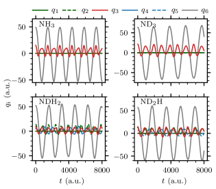
Figure 5: Evolution of the six excited-state normal modes in the four isotopologues of ammonia following electronic excitation at $t=0$. The normal mode coordinates $q_{1}$, $q_{2}$ correspond to the two asymmetric stretching modes, $q_{3}$ to the symmetric stretch, $q_{4}$, $q_{5}$ to the two scissoring modes, and $q_{6}$ to the symmetric bending (i.e., the umbrella vibration) about the minimum of the excited-state PES (see also Fig. 4).

To conclude, we have shown that even the rather simple on-the-fly ab initio thawed Gaussian approximation can capture the key isotope effects in the spectra of ammonia isotopologues. In contrast, the popular global harmonic models can reproduce some of the isotope effects, but inconsistently. The vertical harmonic model, where the PES is computed in the Franck-Condon region, correctly describes the change in the width of the spectral envelope but misses the isotope effect on the peak spacing. The adiabatic harmonic model shows two progressions instead of the single progression observed in experimental spectra. Inspection of the time evolution of excited-state normal modes shows that the single progression in the spectra can be explained by the larger excitation of the symmetric bending mode than of the other modes and by the missing mode effect.^{2, 56} We also show that due to the change of symmetry, in partially deuterated isotopologues additional modes are activated, even though the symmetric bending mode still dominates the dynamics and spectra.

The authors acknowledge the financial support from the European Research Council (ERC) under the European Union’s Horizon 2020 research and innovation program (grant agreement No. 683069 – MOLEQULE) and from the EPFL.

Details of 1D harmonic model calculations, optimized geometries, harmonic frequencies, frequency shifts applied to computed spectra, normal mode evolution for global harmonic models, comparison between on-the-fly TGA and global harmonic model autocorrelation functions, and equation for the calculation of autocorrelation function in Hagedorn’s parametrization.

References

- Born and Oppenheimer 1927 Born, M.; Oppenheimer, R. Zur quantentheorie der molekeln. Ann. d. Phys. 1927, 389, 457–484
- Heller 2018 Heller, E. J. The semiclassical way to dynamics and spectroscopy; Princeton University Press: Princeton, NJ, 2018
- Wilson et al. 1980 Wilson, E.; Decius, J.; Cross, P. Molecular Vibrations: The Theory of Infrared and Raman Vibrational Spectra; Dover Publications, 1980
- Harris and Bertolucci 1989 Harris, D. C.; Bertolucci, M. D. Symmetry and Spectroscopy; Oxford University Press: New York, NY, 1989
- Hazra and Nooijen 2005 Hazra, A.; Nooijen, M. Comparison of various franck-condon and vibronic coupling approaches for simulating electronic spectra: The case of the lowest photoelectron band of ethylene. Phys. Chem. Chem. Phys. 2005, 7, 1759–1771
- Avila Ferrer and Santoro 2012 Avila Ferrer, F. J.; Santoro, F. Comparison of vertical and adiabatic harmonic approaches for the calculation of the vibrational structure of electronic spectra. Phys. Chem. Chem. Phys. 2012, 14, 13549–13563
- Biczysko et al. 2009 Biczysko, M.; Bloino, J.; Barone, V. First Principle Simulation of Vibrationally Resolved Electronic Transition of Phenyl Radical. Chem. Phys. Lett. 2009, 471, 143–147
- Baiardi et al. 2013 Baiardi, A.; Bloino, J.; Barone, V. General Time Dependent Approach to Vibronic Spectroscopy Including Franck-Condon, Herzberg-Teller, and Duschinsky Effects. J. Chem. Theory Comput. 2013, 9, 4097–4115
- Cerezo et al. 2013 Cerezo, J.; Zuniga, J.; Requena, A.; Ávila Ferrer, F. J.; Santoro, F. Harmonic Models in Cartesian and Internal Coordinates to Simulate the Absorption Spectra of Carotenoids at Finite Temperatures. J. Chem. Theory Comput. 2013, 9, 4947–4958
- Begušić et al. 2022 Begušić, T.; Tapavicza, E.; Vaníček, J. Applicability of the Thawed Gaussian Wavepacket Dynamics to the Calculation of Vibronic Spectra of Molecules with Double-Well Potential Energy Surfaces. J. Chem. Theory Comput. 2022, 18, 3065–3074
- Kosloff 1988 Kosloff, R. Time-dependent quantum-mechanical methods for molecular dynamics. J. Phys. Chem. 1988, 92, 2087–2100
- Beck et al. 2000 Beck, M.; Jäckle, A.; Worth, G.; Meyer, H.-D. The multiconfiguration time-dependent Hartree (MCTDH) method: a highly efficient algorithm for propagating wavepackets. Phys. Rep. 2000, 324, 1–105
- Marquardt and Quack 2011 Marquardt, R.; Quack, M. In Handbook of High‐resolution Spectroscopy; Quack, M., Merkt, F., Eds.; John Wiley & Sons, Inc., 2011; pp 511–549
- Tatchen and Pollak 2009 Tatchen, J.; Pollak, E. Semiclassical on-the-fly computation of the absorption spectrum of formaldehyde. J. Chem. Phys. 2009, 130, 041103
- Wehrle et al. 2014 Wehrle, M.; Šulc, M.; Vaníček, J. On-the-fly Ab Initio Semiclassical Dynamics: Identifying Degrees of Freedom Essential for Emission Spectra of Oligothiophenes. J. Chem. Phys. 2014, 140, 244114
- Wehrle et al. 2015 Wehrle, M.; Oberli, S.; Vaníček, J. On-the-fly ab initio semiclassical dynamics of floppy molecules: Absorption and photoelectron spectra of ammonia. J. Phys. Chem. A 2015, 119, 5685
- Gabas et al. 2017 Gabas, F.; Conte, R.; Ceotto, M. On-the-fly Ab Initio Semiclassical Calculation of Glycine Vibrational Spectrum. J. Chem. Theory Comput. 2017, 13, 2378
- Gabas et al. 2018 Gabas, F.; Di Liberto, G.; Conte, R.; Ceotto, M. Protonated glycine supramolecular systems: the need for quantum dynamics. Chem. Sci. 2018, 9, 7894–7901
- Gabas et al. 2019 Gabas, F.; Di Liberto, G.; Ceotto, M. Vibrational investigation of nucleobases by means of divide and conquer semiclassical dynamics. J. Chem. Phys. 2019, 150, 224107
- Bonfanti et al. 2018 Bonfanti, M.; Petersen, J.; Eisenbrandt, P.; Burghardt, I.; Pollak, E. Computation of the S1 S0 vibronic absorption spectrum of formaldehyde by variational Gaussian wavepacket and semiclassical IVR methods. J. Chem. Theory Comput. 2018, 14, 5310–4323
- Patoz et al. 2018 Patoz, A.; Begušić, T.; Vaníček, J. On-the-Fly Ab Initio Semiclassical Evaluation of Absorption Spectra of Polyatomic Molecules beyond the Condon Approximation. J. Phys. Chem. Lett. 2018, 9, 2367–2372
- Begušić et al. 2018 Begušić, T.; Patoz, A.; Šulc, M.; Vaníček, J. On-the-fly ab initio three thawed Gaussians approximation: a semiclassical approach to Herzberg-Teller spectra. Chem. Phys. 2018, 515, 152–163
- Begušić and Vaníček 2020 Begušić, T.; Vaníček, J. On-the-fly ab initio semiclassical evaluation of vibronic spectra at finite temperature. J. Chem. Phys. 2020, 153, 024105
- Golubev et al. 2020 Golubev, N. V.; Begušić, T.; Vaníček, J. On-the-Fly ab initio Semiclassical Evaluation of Electronic Coherences in Polyatomic Molecules Reveals a Simple Mechanism of Decoherence . Phys. Rev. Lett. 2020, 125, 083001
- Prlj et al. 2020 Prlj, A.; Begušić, T.; Zhang, Z. T.; Fish, G. C.; Wehrle, M.; Zimmermann, T.; Choi, S.; Roulet, J.; Moser, J.-E.; Vaníček, J. Semiclassical Approach to Photophysics Beyond Kasha’s Rule and Vibronic Spectroscopy Beyond the Condon Approximation. The Case of Azulene. J. Chem. Theory Comput. 2020, 16, 2617–2626
- Botti et al. 2021 Botti, G.; Ceotto, M.; Conte, R. On-the-fly adiabatically switched semiclassical initial value representation molecular dynamics for vibrational spectroscopy of biomolecules. J. Chem. Phys. 2021, 155, 234102
- Heller 1975 Heller, E. J. Time-dependent approach to semiclassical dynamics. J. Chem. Phys. 1975, 62, 1544–1555
- Grossmann 2006 Grossmann, F. A Semiclassical Hybrid Approach to Many Particle Quantum Dynamics. J. Chem. Phys. 2006, 125, 014111
- Li and Vidal 1994 Li, X.; Vidal, C. R. Predissociation supported high‐resolution vacuum ultraviolet absorption spectroscopy of excited electronic states of NH3. J. Chem. Phys. 1994, 101, 5523–5528
- Chung and Ziegler 1988 Chung, Y. C.; Ziegler, L. D. Rotational hyper‐Raman excitation profiles: Further evidence of J‐dependent subpicosecond dynamics of NH3. J. Chem. Phys. 1988, 89, 4692–4699
- Seideman 1995 Seideman, T. The predissociation dynamics of ammonia: A theoretical study. J. Chem. Phys. 1995, 103, 10556–10565
- Lai et al. 2008 Lai, W.; Lin, S. Y.; Xie, D.; Guo, H. Full-dimensional quantum dynamics of -state photodissociation of ammonia: Absorption spectra. J. Chem. Phys. 2008, 129, 154311
- Ma et al. 2014 Ma, J.; Xie, C.; Zhu, X.; Yarkony, D. R.; Xie, D.; Guo, H. Full-Dimensional Quantum Dynamics of Vibrationally Mediated Photodissociation of NH3 and ND3 on Coupled Ab Initio Potential Energy Surfaces: Absorption Spectra and NH2(A1)/NH2(B1) Branching Ratio. J. Phys. Chem. A 2014, 118, 11926–11934
- Chen et al. 1999 Chen, F.; Judge, D.; Wu, C.; Caldwell, J. Low and room temperature photoabsorption cross sections of NH3 in the UV region. Planet. Space Sci. 1999, 47, 261–266
- Burton et al. 1993 Burton, G. R.; Chan, W. F.; Cooper, G.; Brion, C. E.; Kumar, A.; Meath, W. J. The dipole oscillator strength distribution and predicted dipole properties for ammonia. Can. J. Chem. 1993, 71, 341–351
- Tang et al. 1990 Tang, S. L.; Imre, D. G.; Tannor, D. Ammonia: Dynamical modeling of the absorption spectrum. J. Chem. Phys. 1990, 92, 5919–5934
- Cheng et al. 2006 Cheng, B.; Lu, H.; Chen, H.; Bahou, M.; Lee, Y.; Mebel, A. M.; Lee, L. C.; Liang, M.; Yung, Y. L. Absorption Cross Sections of NH 3 , NH 2 D, NHD 2 , and ND 3 in the Spectral Range 140–220 nm and Implications for Planetary Isotopic Fractionation . Astrophys. Jour. 2006, 647, 1535–1542
- Iachello and Ibrahim 1998 Iachello, F.; Ibrahim, M. Analytic and Algebraic Evaluation of Franck-Condon Overlap Integrals. J. Phys. Chem. A 1998, 102, 9427–9432
- Tannor 2007 Tannor, D. J. Introduction to Quantum Mechanics: A Time-Dependent Perspective; University Science Books: Sausalito, 2007
- Heller 1981 Heller, E. J. The semiclassical way to molecular spectroscopy. Acc. Chem. Res. 1981, 14, 368–375
- Duschinsky 1937 Duschinsky, F. On the Interpretation of Eletronic Spectra of Polyatomic Molecules. Acta Physicochim. U.R.S.S. 1937, 7, 551–566
- Sattasathuchana et al. 2020 Sattasathuchana, T.; Siegel, J. S.; Baldridge, K. K. Generalized Analytic Approach for Determination of Multidimensional Franck–Condon Factors: Simulated Photoelectron Spectra of Polynuclear Aromatic Hydrocarbons. J. Chem. Theory Comput. 2020, 16, 4521–4532
- Vaníček and Begušić 2021 Vaníček, J.; Begušić, T. In Molecular Spectroscopy and Quantum Dynamics; Marquardt, R., Quack, M., Eds.; Elsevier, 2021; pp 199–229
- Lubich 2008 Lubich, C. From Quantum to Classical Molecular Dynamics: Reduced Models and Numerical Analysis, 12th ed.; European Mathematical Society: Zürich, 2008
- Lasser and Lubich 2020 Lasser, C.; Lubich, C. Computing quantum dynamics in the semiclassical regime. Acta Numerica 2020, 29, 229–401
- Hagedorn 1980 Hagedorn, G. A. Semiclassical quantum mechanics. I. The limit for coherent states. Commun. Math. Phys. 1980, 71, 77–93
- Hagedorn 1998 Hagedorn, G. A. Raising and Lowering Operators for Semiclassical Wave Packets. Ann. Phys. (NY) 1998, 269, 77–104
- Kudin and Dymarsky 2005 Kudin, K. N.; Dymarsky, A. Y. Eckart axis conditions and the minimization of the root-mean-square deviation: Two closely related problems. J. Chem. Phys. 2005, 122, 224105
- Kabsch 1978 Kabsch, W. A discussion of the solution for the best rotation to relate two sets of vectors. Acta Cryst. A 1978, 34, 827–828
- Celani and Werner 2003 Celani, P.; Werner, H.-J. Analytical energy gradients for internally contracted second-order multireference perturbation theory. J. Chem. Phys. 2003, 119, 5044–5057
- Roos and Andersson 1995 Roos, B. O.; Andersson, K. Multiconfigurational perturbation theory with level shift — the Cr2 potential revisited. Chem. Phys. Lett. 1995, 245, 215–223
- Werner et al. 2019 Werner, H.-J.; Knowles, P. J.; Knizia, G.; Manby, F. R.; Schütz, M.; Celani, P.; Korona, T.; Lindh, R.; Mitrushenkov, A.; Rauhut, G. et al. MOLPRO, version 2019.2, a package of ab initio programs. 2019; see http://www.molpro.net
- Vaníček 2023 Vaníček, J. Family of Gaussian wavepacket dynamics methods from the perspective of a nonlinear Schrödinger equation. 2023,
- Vaida et al. 1987 Vaida, V.; McCarthy, M. I.; Engelking, P. C.; Rosmus, P.; Werner, H.-J.; Botschwina, P. The ultraviolet absorption spectrum of the transition of jet‐cooled ammonia. J. Chem. Phys. 1987, 86, 6669–6676
- Syage et al. 1992 Syage, J. A.; Cohen, R. B.; Steadman, J. Spectroscopy and dynamics of jet‐cooled hydrazines and ammonia. I. Single‐photon absorption and ionization spectra. J. Chem. Phys. 1992, 97, 6072–6084
- Tutt et al. 1982 Tutt, L.; Tannor, D.; Heller, E. J.; Zink, J. I. The MIME effect: absence of normal modes corresponding to vibronic spacings. Inorg. Chem. 1982, 21, 3858–3859
- Tutt et al. 1987 Tutt, L. W.; Zink, J. I.; Heller, E. J. Simplifying the MIME: A Formula Relating Normal Mode Distortions and Frequencies to the MIME Frequency. Inorg. Chem. 1987, 26, 2158–2160