An Integrated FPGA Accelerator for
Deep Learning-based 2D/3D Path Planning

Abstract

Path planning is a crucial component for realizing the autonomy of mobile robots. However, due to limited computational resources on mobile robots, it remains challenging to deploy state-of-the-art methods and achieve real-time performance. To address this, we propose P3Net (PointNet-based Path Planning Networks), a lightweight deep-learning-based method for 2D/3D path planning, and design an IP core (P3NetCore) targeting FPGA SoCs (Xilinx ZCU104). P3Net improves the algorithm and model architecture of the recently-proposed MPNet. P3Net employs an encoder with a PointNet backbone and a lightweight planning network in order to extract robust point cloud features and sample path points from a promising region. P3NetCore is comprised of the fully-pipelined point cloud encoder, batched bidirectional path planner, and parallel collision checker, to cover most part of the algorithm. On the 2D (3D) datasets, P3Net with the IP core runs 24.54–149.57x and 6.19–115.25x (10.03–59.47x and 3.38–28.76x) faster than ARM Cortex CPU and Nvidia Jetson while only consuming 0.255W (0.809W), and is up to 1049.42x (133.84x) power-efficient than the workstation. P3Net improves the success rate by up to 28.2% and plans a near-optimal path, leading to a significantly better tradeoff between computation and solution quality than MPNet and the state-of-the-art sampling-based methods.

Keywords Path planning  $\cdot$ Neural path planning  $\cdot$ Point cloud processing  $\cdot$ PointNet  $\cdot$ Deep learning  $\cdot$ FPGA

1 Introduction

Path planning aims to find a feasible path from a start to a goal position while avoiding obstacles. It is a fundamental component for mobile robots to autonomously navigate and accomplish a variety of tasks, e.g., farm monitoring [1], aerial package delivery [2], mine exploration [3], and rescue in a collapsed building [4]. Such robotic applications are often deployed on resource-limited edge devices due to severe constraints on the cost and payload. In addition, real-time performance is of crucial importance, since robots may have to plan and update a path on-the-fly in dynamic environments, and delays in path planning would affect the stability of the upstream applications. To cope with the strict performance requirements, FPGA SoCs are increasingly used in robotic applications such as visual odometry [5] and SLAM [6]. FPGA SoC integrates an embedded CPU with a reconfigurable fabric, which allows to develop a custom accelerator tailored for a specific algorithm. Taking these into account, an FPGA-based efficient path planning implementation becomes an attractive solution, which would greatly broaden the application range, since mobile robots can now perform expensive planning tasks on its own without connectivity to remote servers.

Figure 1: Results on the P3Net2D dataset. While MPNet (blue) fails to plan feasible paths in the first two cases, the proposed P3Net (red) plans successfully in all these cases, while reducing the parameters by 32.32x.

Figure 2: Results on the P3Net3D dataset. P3Net (red) produces feasible paths in these cases with 5.43x less parameters than MPNet.

In path planning, the sampling-based methods including Rapidly-exploring Random Tree (RRT) [7] and RRT* [8] are the most prominent, owing to their simplicity and theoretical guarantees. Instead of working on a discretized grid environment like graph-based methods (e.g., A* [9]), these methods explore the environment by incrementally building a tree that represents a set of valid robot motions. While this alleviates the curse of dimensionality to some extent, the computational and memory cost for finding a near-optimal solution is still high, since a sufficient number of tree nodes should be placed to fill the entire free space. A number of RRT variants, e.g., Informed-RRT* [10] and BIT* [11], have been proposed to improve the sampling efficiency and convergence speed. While they offer better tradeoffs between computational effort and solution quality, they rely on carefully designed heuristics, which imply the prior knowledge of the environment and may not be effective in certain scenarios. Due to their increased algorithmic complexity, it even takes up to tens of seconds to complete a task on an embedded CPU. On top of that, their inherently sequential nature would require intricate strategies to map onto a parallel computing platform.

Motivated by the tremendous success of deep learning, the research effort is devoted to developing learning-based methods; the basic idea is to automatically acquire a policy for planning near-optimal paths from a large collection of paths generated by the existing methods. MPNet [12] is a such recently-proposed method. It employs two separate MLP networks for encoding and planning; the former embeds a point cloud representing obstacles into a latent feature space, while the latter predicts a next robot position to incrementally expand a path. Unlike sampling-based methods, MPNet does not involve operations on complex data structures (e.g., KNN search on a K-d tree), and DNN inference is more amenable to parallel processing. This greatly eases the design of a custom processor and makes MPNet a promising candidate for the low-cost FPGA implementation. Its performance is however limited due to the following reasons; the encoder does not take into account the unstructured and unordered nature of point clouds, which degrades the quality of extracted features and eventually results in a lower success rate. Furthermore, the planning network has a lower parameter efficiency, and MPNet has a limited parallelism as it processes only one candidate path at a time until a feasible solution is found.

This paper addresses the above limitations of MPNet and proposes a new learning-based method for 2D/3D path planning, named P3Net (PointNet-based Path Planning Networks), along with its custom IP core for FPGAs (P3NetCore). While the existing methods often assume the availability of abundant computing resources (e.g., GPUs), which is not the case in practice, P3Net is designed to work on resource-limited edge devices and still deliver satisfactory performance. Besides, to our knowledge, P3NetCore is one of the first FPGA-based accelerators for fully learning-based path planning. The main contributions of this paper are summarized as follows:

1. To extract robust features and improve parameter efficiency, we utilize a PointNet [13]-based encoder architecture, which is specifically designed for point cloud processing, together with a lightweight planning network. PointNet is widely adopted as a backbone for point cloud tasks including classification [14] and segmentation [15].

2. We make two algorithmic modifications to MPNet; we introduce a batch planning strategy to process multiple candidate paths in parallel, which offers a new parallelism and improves the success rates without increasing the computation time. We then add a refinement phase at the end to iteratively optimize the path.

3. We design a custom IP core for P3Net, which integrates a fully-pipelined point cloud encoder, a bidirectional neural planner, and a parallelized collision checker. P3Net is developed using High-Level Synthesis (HLS) and implemented on a Xilinx ZCU104 Evaluation Kit.

4. Experimental results validate the effectiveness of the proposed algorithmic optimizations and new models. FPGA-accelerated P3Net achieves significantly better tradeoff between computation time and success rate than MPNet and the state-of-the-art sampling-based methods. It runs up to two orders of magnitude faster than the embedded CPU (ARM Cortex) or integrated CPU-GPU systems (Nvidia Jetson). P3Net quickly converges to near-optimal solutions in most cases, and is up to three orders of magnitude more power-efficient than the workstation.

The rest of the paper is structured as follows: Section 2 provides a brief overview of the related works, while Section 3 covers the preliminaries. The proposed P3Net is explained in Section 4, and Section 5 elaborates on the design and implementation of P3NetCore. Experimental results are presented in Section 6, and Section 7 concludes the paper.

2 Related Works

2.1 Sampling and Learning-based Path Planning

The sampling-based methods, e.g., RRT [7] and its provably asymptotically-optimal version, RRT* [8], are prevalent in robotic path planning; they explore the environment by incrementally growing an exploration tree. Considering that the free space should be densely filled with tree nodes to find a high-quality solution, the computational complexity is at worst exponential with respect to the space dimension and may be intractable in some difficult cases such as the environments with narrow passages. The later methods introduce various heuristics to improve search efficiency; Informed-RRT* [10] uses an ellipsoidal heuristic, while BIT* [11] and its variants [16, 17] apply graph-search techniques. Despite the steady improvement, they still rely on sophisticated heuristics; deep learning-based methods have been extensively studied to automatically learn effective policies for planning high-quality paths.

Several studies have investigated the hybrid approach, where deep learning techniques are incorporated into the classical planners. Ichter et al. [18, 19] and Wang et al. [20] extend RRT by generating informed samples from a learned latent space. Neural A* [21] is a differentiable version of A*, while WPN [22] uses LSTM to generate path waypoints and then A* to connect them. Aside from the hybrid approach, an end-to-end approach aims to directly learn the behavior of classical planners via supervised learning; Inoue et al. [23] and Bency et al. [24] train LSTM networks on the RRT* and A*-generated paths, respectively. CNN [25], PointNet [26, 27], and Transformer [28, 29, 30] are also employed to construct end-to-end models.

MPNet and our P3Net follow the end-to-end supervised approach, and perform path planning on a continuous domain by directly regressing coordinates of the path points. P3Net is unique in that it puts more emphasis on the computational and resource efficiency and builds upon a lightweight MLP network, making it suitable for deployment on the low-end edge devices. Besides, the environment is represented by a space-efficient sparse point cloud as in [31, 26, 27], unlike the grid map which introduces quantization errors and leads to a large memory consumption, as it contains redundant grid cells for the free space and its size increases exponentially with respect to space dimensionality.

2.2 Hardware Acceleration of Path Planning

Several works have explored the FPGA and ASIC acceleration of the conventional graph and sampling-based methods, e.g., A* [32, 33, 34, 35] and RRT [36, 37, 38, 39]. Kosuge et al. [33] develops an accelerator for A* graph construction and search on the Xilinx ZCU102. Since A* operates on grid environments and is subject to the curse of dimensionality, it is challenging to handle higher dimensional cases or larger maps. For RRT-family algorithms, Malik et al. [36] proposes a parallelized architecture for RRT, which first partitions the workspace into grids and distributes them across multiple RRT processes. This approach involves redundant computations as some RRT processes may explore irrelevant regions for a given problem. Xiao et al. [37, 38] proposes an FPGA accelerator for RRT* that runs tree expansion and rewiring steps in a pipelined manner. Chung et al. [39] devises a dual-tree RRT with parallel and greedy tree expansion for ASIC implementation.

Some studies leverage GPU [40] or distributed computing techniques [41, 42] to speed up RRT, while it degrades power efficiency and not suitable for battery-powered edge devices. In [40], collision checks between obstacles and a robot arm are parallelized on GPU; Devaurs et al. [41] employs a large-scale distributed memory architecture and a message passing interface. RRT-family algorithms repeat tree expansion and rewiring steps alternately; they are inherently sequential and difficult to accelerate without a sophisticated technique (e.g., space subdivision, parallel tree expansion). In contrast, our proposed P3Net offers more parallelism and is hardware-friendly, as it mainly consists of DNN inferences, and does not operate on complex data structures (e.g., sorting, KNN on K-d trees, graph search).

Only a few works [43, 44, 45] have considered the hardware acceleration of neural planners. Huang et al. [44] presents an accelerator for a sampling-based method with a CNN model, which produces a probability map given an image of the environment for sampling the next robot position. In [45], an RTL design of a Graph Neural Network-based path explorer rapidly evaluates priority scores for edges in a random geometric graph, and edges with high priority are selected to form a path. This paper extends our previous work [43]; instead of only accelerating the DNN inference in MPNet, we implement the whole bidirectional planning algorithm on FPGA. In addition, we derive a new path planning method, P3Net, to achieve both higher success rate and speedup. This paper is one of the first to realize a real-time fully learning-based path planner on a resource-limited FPGA device.

3 Preliminaries: MPNet

In this section, we briefly describe the MPNet [12] algorithm (Alg. 1), which serves as a basis of our proposal.

3.1 Notations and Overview of MPNet

Let us consider a robot moving around in a 2D/3D environment $\mathcal{X}\subset\mathbb{R}^{D}$ ($D=2,3$). For simplicity, the robot is modeled as a point-mass, and its state (configuration) is a position $\mathbf{c}\in\mathbb{R}^{D}$. Note that MPNet is a general framework and can be applied to a wide range of problem settings. Given a pair of start and goal points $\mathbf{c}_{\mathrm{start}},\mathbf{c}_{\mathrm{goal}}\in\mathbb{R}^{D}$, MPNet tries to find a collision-free path $\tau=\left\{\mathbf{c}_{0},\mathbf{c}_{1},\ldots,\mathbf{c}_{T}\right\}$ ($\mathbf{c}_{0},\mathbf{c}_{T}=\mathbf{c}_{\mathrm{start}},\mathbf{c}_{\mathrm{goal}}$) if exists. As illustrated in Fig. 3 (left), MPNet assumes that obstacle information is represented as a point cloud $\mathcal{P}=\left\{\mathbf{p}_{0},\ldots,\mathbf{p}_{N-1}\right\}\in\mathbb{R}^{N\times 3}$ containing $N$ points uniformly sampled from the obstacle region. The notation $\tau\xleftarrow{+}\mathbf{c}$ is a shorthand for $\tau\leftarrow\tau\cup\left\{\mathbf{c}\right\}$.

Importantly, MPNet uses two DNN models for encoding and planning, namely ENet and PNet (Fig. 3 (right)); ENet compresses the obstacle information $\mathcal{P}$ into a feature embedding $\bm{\phi}(\mathcal{P})\in\mathbb{R}^{M}$. PNet is responsible for sampling the next position $\mathbf{c}_{t+1}$ which is one step closer to the goal, from the current and goal positions $\mathbf{c}_{t},\mathbf{c}_{\mathrm{goal}}$ as well as the obstacle feature $\bm{\phi}(\mathcal{P})$. Fig. 4 outlines the algorithm. MPNet consists of two main steps, referred to as (1) initial coarse planning and (2) replanning, plus (3) a final smoothing step, which are described in the following sections.

3.2 MPNet Algorithm

MPNet first extracts a feature $\bm{\phi}(\mathcal{P})$ (Alg. 1, line 3) and proceeds to the initial coarse planning step (line 5) to roughly plan a path $\tau$ between start and goal points $\mathbf{c}_{\mathrm{start}},\mathbf{c}_{\mathrm{goal}}$. The bidirectional planning with PNet, referred to as $\mathrm{NeuralPlanner}$ (lines 15-26), plays a central role in this step, which is described as follows.

Given a pair of start-goal points $\mathbf{c}_{s},\mathbf{c}_{g}$, $\mathrm{NeuralPlanner}$ plans two paths $\tau^{\mathrm{a}},\tau^{\mathrm{b}}$ in forward and reverse directions alternately (lines 19, 22). The forward path $\tau^{\mathrm{a}}=\left\{\mathbf{c}_{s},\ldots,\mathbf{c}_{\mathrm{end}}^{\mathrm{a}}\right\}$ is incrementally expanded from start to goal by repeating the PNet inference (lines 20-21). From the current path endpoint $\mathbf{c}_{\mathrm{end}}^{\mathrm{a}}$ and goal $\mathbf{c}_{g}$, PNet computes a new waypoint $\mathbf{c}_{\mathrm{new}}^{\mathrm{a}}$, which becomes a new endpoint of $\tau^{\mathrm{a}}$ and used as input in the next inference. Similarly, the backward path $\tau^{\mathrm{b}}=\left\{\mathbf{c}_{g},\ldots,\mathbf{c}_{\mathrm{end}}^{\mathrm{b}}\right\}$ is expanded from goal to start. In this case, PNet computes a next position $\mathbf{c}_{\mathrm{new}}^{\mathrm{b}}$ from an input $\left[\bm{\phi}(\mathcal{P}),\mathbf{c}_{\mathrm{end}}^{\mathrm{b}},\mathbf{c}_{s}\right]$ to get closer to the start position $\mathbf{c}_{s}$ (lines 23-24). Note that the newly added edge $(\mathbf{c}_{\mathrm{end}}^{\mathrm{a}},\mathbf{c}_{\mathrm{new}}^{\mathrm{a}})$ (or $(\mathbf{c}_{\mathrm{end}}^{\mathrm{b}},\mathbf{c}_{\mathrm{new}}^{\mathrm{b}})$) may be in collision; such edge is removed in the later replanning step. After updating $\tau^{\mathrm{a}}$ or $\tau^{\mathrm{b}}$, $\mathrm{NeuralPlanner}$ attempts to connect them and create a path $\tau=\left\{\mathbf{c}_{0},\mathbf{c}_{1},\ldots,\mathbf{c}_{T}\right\}$ between $\mathbf{c}_{0},\mathbf{c}_{T}=\mathbf{c}_{s},\mathbf{c}_{g}$, if there is no obstacle between path endpoints $\mathbf{c}_{\mathrm{end}}^{\mathrm{a}},\mathbf{c}_{\mathrm{end}}^{\mathrm{b}}$ (line 25). The above process, i.e., path expansion and collision checking, is repeated until a feasible path is obtained or the maximum number of iterations $I$ is reached. The algorithm fails if $\tau^{\mathrm{a}},\tau^{\mathrm{b}}$ cannot be connected after $I$ iterations (line 26).

The tentative path $\tau$ connecting $\mathbf{c}_{\mathrm{start}},\mathbf{c}_{\mathrm{goal}}$ is obtained from $\mathrm{NeuralPlanner}$ (line 5); if $\tau$ passes the collision check, then MPNet performs smoothing and returns it as a final solution (lines 7-8). In the smoothing process (Fig. 4 (right)), the planner greedily prunes redundant waypoints from $\tau$ to obtain a shorter and smoother path; given three waypoints $\mathbf{c}_{i},\mathbf{c}_{j},\mathbf{c}_{k}$ ($i<j<k$), the intermediate one $\mathbf{c}_{j}$ is dropped if $\mathbf{c}_{i}$ and $\mathbf{c}_{k}$ can be directly connected by a straight line. This involves a collision checking on the new edge $(\mathbf{c}_{i},\mathbf{c}_{k})$.

As already mentioned, the initial solution $\tau$ may contain edges that collide with obstacles (Fig. 4 (left, red lines)); if this is the case, the planner moves on to the replanning process (lines 11, 27-36). For every edge $\mathbf{c}_{i},\mathbf{c}_{i+1}\in\tau$ that is in collision, MPNet tries to plan an alternative sub-path $\tau_{i,i+1}=\{\mathbf{c}_{i},\mathbf{c}_{i}^{(1)},\mathbf{c}_{i}^{(2)},\ldots,\mathbf{c}_{i+1}\}$ between $\mathbf{c}_{i},\mathbf{c}_{i+1}$ to avoid obstacles (Fig. 4 (center), line 33). $\mathrm{NeuralPlanner}$ is again called with $\mathbf{c}_{i},\mathbf{c}_{i+1}$ as input start-goal points. The replanning fails if $\mathrm{NeuralPlanner}$ cannot plan a detour. The new intermediate waypoints $\mathbf{c}_{i}^{(1)},\mathbf{c}_{i}^{(2)},\ldots$ are then inserted to the path (line 35). If the resultant path is collision-free, MPNet returns it as a solution after smoothing (lines 12-13); otherwise, it runs the replanning again. In this way, MPNet gradually removes the non-collision-free edges from the solution. Replanning is repeated for $I_{\mathrm{Replan}}$ times at maximum, and MPNet fails if a feasible solution is not obtained (line 14).

One notable feature of MPNet is that, PNet exhibits a stochastic behavior as it utilizes dropout in the inference phase, unlike the typical case where the dropout is only enabled during training. PNet inference $\left[\bm{\phi}(\mathcal{P}),\mathbf{c}_{t},\mathbf{c}_{\mathrm{goal}}\right]\mapsto\mathbf{c}_{t+1}$ is hence viewed as sampling the next position $\mathbf{c}_{t+1}$ from a learned distribution $p(\bm{\phi}(\mathcal{P}),\mathbf{c}_{t})$ parameterized by a planning environment $\bm{\phi}(\mathcal{P})$ and a current position $\mathbf{c}_{t}$, which represents a promising region around an optimal path from $\mathbf{c}_{t}$ to $\mathbf{c}_{\mathrm{goal}}$. Such dropout sampling (Monte Carlo dropout) was first proposed in [46] as an efficient way to estimate the uncertainty in Bayesian Neural Networks (BNNs). As both $\mathrm{NeuralPlanner}$ and $\mathrm{Replan}$ rely on PNet, they are also non-deterministic and produce different results on the same input. As a result, MPNet generates different candidate paths in the replanning phase, leading to an increased chance of avoiding obstacles and higher success rate.

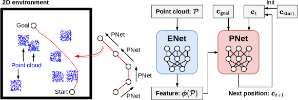
Figure 3: Overview of the MPNet algorithm. MPNet takes as input start-goal positions $\mathbf{c}_{\mathrm{start}},\mathbf{c}_{\mathrm{goal}}$ as well as a point cloud $\mathcal{P}$ representing obstacles in the environment (blue points). MPNet employs two DNNs, ENet and PNet, for feature extraction and planning. ENet extracts a feature $\bm{\phi}(\mathcal{P})$ from the point cloud, while PNet computes waypoints one at a time and incrementally builds a path from $\mathbf{c}_{\mathrm{start}}$ to $\mathbf{c}_{\mathrm{goal}}$. Given $\bm{\phi}(\mathcal{P})$, $\mathbf{c}_{\mathrm{goal}}$, and a current position $\mathbf{c}_{t}$ (path endpoint), PNet computes the next position $\mathbf{c}_{t+1}$ to make a step forward to the goal.

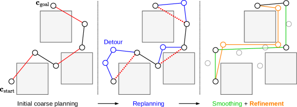
Figure 4: Processing flow of the MPNet path planning. MPNet mainly consists of three steps. initial coarse planning step (left): MPNet roughly plans a path connecting start-goal points, which may not be collision-free (red edges). Replanning step (center): MPNet removes the edges colliding with obstacles from the initial path and replaces them with alternative edges (detours, blue) to obtain a collision-free path. Smoothing step (right): The redundant waypoints (semi-transparent points) are pruned to obtain a smooth and straight path (green edges). Our proposed method, P3Net, performs an additional Refinement step (right) to gradually improve the solution (orange edges).

Algorithm 1 MPNet for 2D and 3D path planning

1:Start $\mathbf{c}_{\mathrm{start}}$, goal $\mathbf{c}_{\mathrm{goal}}$, obstacle point cloud $\mathcal{P}$

2:Path $\tau=\left\{\mathbf{c}_{0},\mathbf{c}_{1},\ldots,\mathbf{c}_{T}\right\}$ ($\mathbf{c}_{0},\mathbf{c}_{T}=\mathbf{c}_{\mathrm{start}},\mathbf{c}_{\mathrm{goal}}$)

3:$\bm{\phi}(\mathcal{P})\leftarrow\mathrm{ENet}(\mathcal{P})$ $\triangleright$ Point cloud feature extraction

4:$\triangleright$ Initial coarse planning

5:$\tau\leftarrow\mathrm{NeuralPlanner}(\mathbf{c}_{\mathrm{start}},\mathbf{c}_{\mathrm{goal}},\bm{\phi}(\mathcal{P}))$

6:if $\tau=\varnothing$ : return $\varnothing$ $\triangleright$ Failure

7:$\tau\leftarrow\mathrm{Smoothing}(\tau)$

8:if $\tau$ is collision-free : return $\tau$ $\triangleright$ Success

9:$\triangleright$ Replanning

10:for $i=0,\ldots,I_{\mathrm{Replan}}-1$ do

11:     $\tau\leftarrow\mathrm{Replan}(\tau,\bm{\phi}(\mathcal{P}))$

12:     $\tau\leftarrow\mathrm{Smoothing}(\tau)$

13:     if $\tau\neq\varnothing$ and $\tau$ is collision-free : return $\tau$ $\triangleright$ Success

14:return $\varnothing$ $\triangleright$ Failure

15:function $\mathrm{NeuralPlanner}$($\mathbf{c}_{s},\mathbf{c}_{g},\bm{\phi}(\mathcal{P})$)

16:     $\tau^{\mathrm{a}}\leftarrow\left\{\mathbf{c}_{s}\right\},\ \tau^{\mathrm{b}}\leftarrow\left\{\mathbf{c}_{g}\right\}$ $\triangleright$ Forward-backward paths

17:     $\mathbf{c}_{\mathrm{end}}^{\mathrm{a}}\leftarrow\mathbf{c}_{s},\ \mathbf{c}_{\mathrm{end}}^{\mathrm{b}}\leftarrow\mathbf{c}_{g},\ r=0$ $\triangleright$ Path endpoints

18:     for $i=0,\ldots,I-1$ do

19:         if $r=0$ : $\triangleright$ Forward direction (start to goal)

20:              $\mathbf{c}_{\mathrm{new}}^{\mathrm{a}}\leftarrow\mathrm{PNet}(\bm{\phi}(\mathcal{P}),\mathbf{c}_{\mathrm{end}}^{\mathrm{a}},\mathbf{c}_{g})$

21:              $\tau^{\mathrm{a}}\xleftarrow{+}\left\{\mathbf{c}_{\mathrm{new}}^{\mathrm{a}}\right\},\ \mathbf{c}_{\mathrm{end}}^{\mathrm{a}}\leftarrow\mathbf{c}_{\mathrm{new}}^{\mathrm{a}},\ r=1$

22:         else if $r=1$ : $\triangleright$ Reverse direction (goal to start)

23:              $\mathbf{c}_{\mathrm{new}}^{\mathrm{b}}\leftarrow\mathrm{PNet}(\bm{\phi}(\mathcal{P}),\mathbf{c}_{\mathrm{end}}^{\mathrm{b}},\mathbf{c}_{s})$

24:              $\tau^{\mathrm{b}}\xleftarrow{+}\left\{\mathbf{c}_{\mathrm{new}}^{\mathrm{b}}\right\},\ \mathbf{c}_{\mathrm{end}}^{\mathrm{b}}\leftarrow\mathbf{c}_{\mathrm{new}}^{\mathrm{b}},\ r=0$          

25:         if $\tau^{\mathrm{a}}$ and $\tau^{\mathrm{b}}$ are connectable : return $\tau=\left\{\tau^{\mathrm{a}},\tau^{\mathrm{b}}\right\}$      

26:     return $\varnothing$ $\triangleright$ Failure

27:function $\mathrm{Replan}$($\tau=\left\{\mathbf{c}_{0},\ldots,\mathbf{c}_{T}\right\},\bm{\phi}(\mathcal{P})$)

28:     $\tau_{\mathrm{new}}\leftarrow\varnothing$

29:     for $i=0,\ldots,T-1$ do

30:         if $\mathbf{c}_{i}$ and $\mathbf{c}_{i+1}$ are connectable :

31:              $\tau_{\mathrm{new}}\xleftarrow{+}\left\{\mathbf{c}_{i},\mathbf{c}_{i+1}\right\}$

32:         else$\triangleright$ Plan a detour $\tau_{i,i+1}=\{\mathbf{c}_{i},\mathbf{c}_{i}^{(1)},\mathbf{c}_{i}^{(2)},\ldots,\mathbf{c}_{i+1}\}$

33:              $\tau_{i,i+1}\leftarrow\mathrm{NeuralPlanner}(\mathbf{c}_{i},\mathbf{c}_{i+1},\bm{\phi}(\mathcal{P}))$

34:              if $\tau_{i,i+1}=\varnothing$ : return $\varnothing$ $\triangleright$ Failure

35:              $\tau_{\mathrm{new}}\xleftarrow{+}\tau_{i,i+1}$          

36:         return $\tau_{\mathrm{new}}$ $\triangleright$ Success      

4 Method: P3Net

In this section, we propose a new path planning algorithm, P3Net (Algs. 2-3), by making improvements to the algorithm and model architecture of MPNet.

4.1 Algorithmic Improvements

P3Net introduces two ideas, (1) batch planning and (2) refinement step, into the MPNet algorithm. As depicted in Figs. 4–5, P3Net (1) estimates multiple paths at the same time to increase the parallelism, and (2) iteratively refines the obtained path to improve its quality.

4.1.1 Batch Planning

According to the $\mathrm{NeuralPlanner}$ algorithm in MPNet (Alg. 1, lines 15-26), forward-backward paths $\tau_{a},\tau_{b}$ are incrementally expanded from start-goal points $\mathbf{c}_{s},\mathbf{c}_{g}$ until their endpoints $\mathbf{c}_{\mathrm{end}}^{\mathrm{a}},\mathbf{c}_{\mathrm{end}}^{\mathrm{b}}$ are connectable. In this process, PNet computes a single next position $\mathbf{c}_{\mathrm{new}}^{\mathrm{a}}$ ($\mathbf{c}_{\mathrm{new}}^{\mathrm{b}}$) from a current endpoint $\mathbf{c}_{\mathrm{end}}^{\mathrm{a}}$ ($\mathbf{c}_{\mathrm{end}}^{\mathrm{b}}$) and the destination $\mathbf{c}_{g}$ ($\mathbf{c}_{s}$) (lines 20, 23). Due to the input batch size of one, PNet cannot fully utilize the parallel computing capability of CPU/GPUs, and also suffers from the kernel launch overheads and frequent data transfers. To amortize this overhead, two PNet inferences (lines 20, 23) can be merged into one with a batch size of two, i.e., two next positions $\left[\mathbf{c}_{s},\mathbf{c}_{g}\right]$ are computed at once from concatenated inputs $\left[\mathbf{c}_{\mathrm{end}}^{\mathrm{a}},\mathbf{c}_{\mathrm{end}}^{\mathrm{b}}\right],\left[\mathbf{c}_{g},\mathbf{c}_{s}\right]$.

As shown in Fig. 5, our $\mathrm{NeuralPlannerEx}$ algorithm (Alg. 3, lines 1-26) takes this idea further by creating a total of $B$ pairs of forward-backward paths (i.e., $\tau_{\mathcal{B}}^{\mathrm{a}}=\left[\tau_{0}^{\mathrm{a}},\ldots,\tau_{B-1}^{\mathrm{a}}\right]$, $\tau_{\mathcal{B}}^{\mathrm{b}}=\left[\tau_{0}^{\mathrm{b}},\ldots,\tau_{B-1}^{\mathrm{b}}\right]$). It serves as a drop-in replacement for $\mathrm{NeuralPlanner}$. It keeps track of the forward-backward path pairs $(\tau_{\mathcal{B}}^{\mathrm{a}},\tau_{\mathcal{B}}^{\mathrm{b}})$, which are initialized with start-goal points (lines 7-8), as well as path lengths $\ell_{\mathcal{B}}$ (initialized with all ones, line 9), path endpoints $\mathbf{C}_{\mathcal{B}}$, and corresponding destination points $\mathbf{C}_{\mathcal{B}}^{\mathrm{goal}}$ (lines 3-5).

In each iteration $i$, PNet takes $(\bm{\phi}(\mathcal{P}),\mathbf{C}_{\mathcal{B}},\mathbf{C}_{\mathcal{B}}^{\mathrm{goal}})$ as input and computes the next waypoints $\mathbf{C}_{\mathcal{B}}^{\mathrm{next}}=[\mathbf{c}_{0}^{\mathrm{a},i+1},\mathbf{c}_{0}^{\mathrm{b},i+1},\ldots,\mathbf{c}_{B-1}^{\mathrm{a},i+1},\mathbf{c}_{B-1}^{\mathrm{b},i+1}]$ for a batch of paths within one inference step (line 11), resulting in a total batch size of $2B$. Note that $\mathbf{c}_{j}^{\mathrm{a},i+1},\mathbf{c}_{j}^{\mathrm{b},i+1}$ denote $i+1$-th waypoints in $j$-th forward-backward paths ($j\in\left[0,B\right)$). Then, for each sample $j$, the algorithm tries to connect a path pair $\tau_{j}^{\mathrm{a}},\tau_{j}^{\mathrm{b}}$, by checking whether any of the three lines connecting $(\mathbf{c}_{j}^{\mathrm{a},i+1},\mathbf{c}_{j}^{\mathrm{b},i})$, $(\mathbf{c}_{j}^{\mathrm{a},i},\mathbf{c}_{j}^{\mathrm{b},i+1})$, and $(\mathbf{c}_{j}^{\mathrm{a},i+1},\mathbf{c}_{j}^{\mathrm{b},i+1})$ is obstacle-free and hence passable (lines 13-21). If this check passes, $\tau_{j}^{\mathrm{a}}$ and $\tau_{j}^{\mathrm{b}}$ are concatenated and the result $\tau=\left[\mathbf{c}_{s},\mathbf{c}_{s}^{\mathrm{a},1},\ldots,\mathbf{c}_{s}^{\mathrm{b},1},\mathbf{c}_{g}\right]$ is returned to the caller (line 24, blue path in Fig. 5); otherwise, the algorithm updates the current endpoints $\mathbf{C}_{\mathcal{B}}$ with the new ones $\mathbf{C}_{\mathcal{B}}^{\mathrm{next}}$ and proceeds to the next iteration. $\mathbf{C}_{\mathcal{B}}^{\mathrm{next}}$ is also used to update the paths $\tau_{\mathcal{B}}^{\mathrm{a}},\tau_{\mathcal{B}}^{\mathrm{b}}$ accordingly (lines 22-23). It fails if no solution is found after the maximum number of iterations $I$.

$\mathrm{NeuralPlannerEx}$ is more likely to find a solution compared to $\mathrm{NeuralPlanner}$, as it creates $B$ candidate paths for a given task. This allows the replanning process (Alg. 2, lines 11-16), which repetitively calls $\mathrm{NeuralPlannerEx}$, to complete in a less number of trials, leading to higher success rates as confirmed in the evaluation (Sec. 6.3). To further improve success rates, P3Net runs the initial coarse planning for $I_{\mathrm{Init}}\geq 1$ times (Alg. 2, lines 5-8), as opposed to MPNet which immediately fails when a feasible path is not obtained in the first attempt (Alg. 1, lines 5, 6).

4.1.2 Refinement Step

The paths generated by MPNet may not be optimal, since it returns a first found path in an initial coarse planning or a replanning phase. As highlighted in Alg. 2, lines 18-23, the refinement phase is added at the end of P3Net to gradually improve the quality of output paths (Fig. 5). For a fixed number of iterations $I_{\mathrm{Refine}}$, it computes a new collision-free path $\tau_{\mathrm{new}}$ based on the current solution $\tau_{\mathrm{best}}$ (with a cost of $c_{\mathrm{best}}$) using $\mathrm{Refine}$ algorithm (Alg. 3, lines 27-36), and accepts $\tau_{\mathrm{new}}$ as a new solution if it lowers the cost ($c_{\mathrm{new}}<c_{\mathrm{best}}$). Same as the replanning phase, $\mathrm{Refine}$ also relies on $\mathrm{NeuralPlannerEx}$ at its core. It takes the collision-free path $\tau$ as an input and builds a new path $\tau_{\mathrm{new}}$ as follows: for every edge $(\mathbf{c}_{i},\mathbf{c}_{i+1})\in\tau$, it plans a path $\tau_{i,i+1}$ using $\mathrm{NeuralPlannerEx}$ (line 30) and connects $\mathbf{c}_{i},\mathbf{c}_{i+1}$ with $\tau_{i,i+1}$ if it is collision-free (line 33). The evaluation results (Sec. 6.5) confirm that it converges to the optimal solution in most cases. Note that MPNet can be viewed as a special case of P3Net with $B=1$, $I_{\mathrm{Init}}=1$, and $I_{\mathrm{Refine}}=0$.

Algorithm 2 P3Net (changed parts are highlighted in red)

1:Start $\mathbf{c}_{\mathrm{start}}$, goal $\mathbf{c}_{\mathrm{goal}}$, obstacle point cloud $\mathcal{P}$

2:Path $\tau=\left\{\mathbf{c}_{0},\ldots,\mathbf{c}_{T}\right\}$ ($\mathbf{c}_{0},\mathbf{c}_{T}=\mathbf{c}_{\mathrm{start}},\mathbf{c}_{\mathrm{goal}}$)

3:Compute point cloud feature: $\bm{\phi}(\mathcal{P})\leftarrow\mathrm{ENet}(\mathcal{P})$

4:$\triangleright$ Initial coarse planning

5:for $i=0,\ldots,I_{\mathrm{Init}}-1$ do

6:     $\tau\leftarrow\mathrm{NeuralPlannerEx}(\mathbf{c}_{\mathrm{start}},\mathbf{c}_{\mathrm{goal}},\bm{\phi}(\mathcal{P}))$

7:     if $\tau\neq\varnothing$ : break$\triangleright$ Success

8:if $\tau=\varnothing$ : return $\varnothing$ $\triangleright$ Failure

9:$\tau\leftarrow\mathrm{Smoothing}(\tau)$

10:$\triangleright$ Replanning

11:if $\tau$ is not collision-free :

12:     for $i=0,\ldots,I_{\mathrm{Replan}}-1$ do

13:         $\tau\leftarrow\mathrm{Replan}(\tau,\bm{\phi}(\mathcal{P}))$

14:         $\tau\leftarrow\mathrm{Smoothing}(\tau)$

15:         if $\tau\neq\varnothing$ and $\tau$ is collision-free : break$\triangleright$ Success      

16:     if $\tau=\varnothing$ : return $\varnothing$ $\triangleright$ Failure

17:$\triangleright$ Refinement

18:$\tau_{\mathrm{best}}\leftarrow\tau,\ c_{\mathrm{best}}\leftarrow$ Cost($\tau_{\mathrm{best}}$) $\triangleright$ $\tau$ is now collision-free

19:for $i=0,\ldots,I_{\mathrm{Refine}}-1$ do

20:     $\tau_{\mathrm{new}}\leftarrow$ Refine($\tau_{\mathrm{best}},\bm{\phi}(\mathcal{P})$)

21:     $\tau_{\mathrm{new}}\leftarrow$ Smoothing($\tau_{\mathrm{new}}$)

22:     $c_{\mathrm{new}}\leftarrow$ Cost($\tau_{\mathrm{new}}$)

23:     if $c_{\mathrm{new}}<c_{\mathrm{best}}$ : $c_{\mathrm{best}}=c_{\mathrm{new}},\ \tau_{\mathrm{best}}=\tau_{\mathrm{new}}$

24:return $\tau_{\mathrm{best}}$

Algorithm 3 Batch Planning and Refinement Step in P3Net

1:function $\mathrm{NeuralPlannerEx}$($\mathbf{c}_{s},\mathbf{c}_{g},\bm{\phi}(\mathcal{P})$)

2:$\triangleright$ Initialize batch of current and goal positions

3:     $\mathbf{C}_{\mathcal{B}}\leftarrow\left[\mathbf{c}_{0}^{\mathrm{a,0}},\mathbf{c}_{0}^{\mathrm{b,0}},\ldots,\mathbf{c}_{B-1}^{\mathrm{a,0}},\mathbf{c}_{B-1}^{\mathrm{b,0}}\right]\in\mathbb{R}^{2B\times D}$

4:         ($\forall j\ \mathbf{c}_{j}^{\mathrm{a,0}}=\mathbf{c}_{s},\mathbf{c}_{j}^{\mathrm{b,0}}=\mathbf{c}_{g}$)

5:     $\mathbf{C}_{\mathcal{B}}^{\mathrm{goal}}\leftarrow\left[\mathbf{c}_{g},\mathbf{c}_{s},\mathbf{c}_{g},\mathbf{c}_{s},\ldots,\mathbf{c}_{g},\mathbf{c}_{s}\right]\in\mathbb{R}^{2B\times D}$

6:$\triangleright$ Initialize batch of paths and lengths

7:     $\tau_{\mathcal{B}}^{\mathrm{a}}\leftarrow\left[\tau_{0}^{\mathrm{a}},\tau_{1}^{\mathrm{a}},\ldots,\tau_{B-1}^{\mathrm{a}}\right],\ \forall j\ \tau_{j}^{\mathrm{a}}=\left\{\mathbf{c}_{s}\right\}$

8:     $\tau_{\mathcal{B}}^{\mathrm{b}}\leftarrow\left[\tau_{0}^{\mathrm{b}},\tau_{1}^{\mathrm{b}},\ldots,\tau_{B-1}^{\mathrm{b}}\right],\ \forall j\ \tau_{j}^{\mathrm{b}}=\left\{\mathbf{c}_{g}\right\}$

9:     $\ell_{\mathcal{B}}\leftarrow\left[\ell_{0}^{\mathrm{a}},\ell_{0}^{\mathrm{b}},\ldots,\ell_{B-1}^{\mathrm{a}},\ell_{B-1}^{\mathrm{b}}\right],\ \forall j\ \ell_{j}^{\mathrm{x}}=|\tau_{j}^{\mathrm{x}}|=1$

10:     for $i=0,\ldots,I-1$ do

11:         $\mathbf{C}_{\mathcal{B}}^{\mathrm{next}}\leftarrow$ PNet($\bm{\phi}(\mathcal{P}),\mathbf{C}_{\mathcal{B}},\mathbf{C}_{\mathcal{B}}^{\mathrm{goal}}$) $\triangleright$ Next positions

12:         ($\mathbf{C}_{\mathcal{B}}^{\mathrm{next}}=\left[\mathbf{c}_{0}^{\mathrm{a},i+1},\mathbf{c}_{0}^{\mathrm{b},i+1},\ldots,\mathbf{c}_{B-1}^{\mathrm{a},i+1},\mathbf{c}_{B-1}^{\mathrm{b},i+1}\right]$)

13:         for $j=0,\ldots,B-1$ do $\triangleright$ Collision checks

14:              if ($\mathbf{c}_{j}^{\mathrm{a},i+1},\mathbf{c}_{j}^{\mathrm{b},i}$) are connectable :

15:                  $\mathrm{expandA}\leftarrow 1,\ \mathrm{expandB}\leftarrow 0,\ s\leftarrow 1$

16:              else if ($\mathbf{c}_{j}^{\mathrm{a},i},\mathbf{c}_{j}^{\mathrm{b},i+1}$) are connectable :

17:                  $\mathrm{expandA}\leftarrow 0,\ \mathrm{expandB}\leftarrow 1,\ s\leftarrow 1$

18:              else if ($\mathbf{c}_{j}^{\mathrm{a},i+1},\mathbf{c}_{j}^{\mathrm{b},i+1}$) are connectable :

19:                  $\mathrm{expandA}\leftarrow 1,\ \mathrm{expandB}\leftarrow 1,\ s\leftarrow 1$

20:              else

21:                  $\mathrm{expandA}\leftarrow 1,\ \mathrm{expandB}\leftarrow 1,\ s\leftarrow 0$               

22:              if $\mathrm{expandA}$ : $\tau_{j}^{\mathrm{a}}\xleftarrow{+}\{\mathbf{c}_{j}^{\mathrm{a},i+1}\},\ \ell_{j}^{\mathrm{a}}\leftarrow\ell_{j}^{\mathrm{a}}+1$

23:              if $\mathrm{expandB}$ : $\tau_{j}^{\mathrm{b}}\xleftarrow{+}\{\mathbf{c}_{j}^{\mathrm{b},i+1}\},\ \ell_{j}^{\mathrm{b}}\leftarrow\ell_{j}^{\mathrm{b}}+1$

24:              if $s=1$ : return $\tau=\left\{\tau_{j}^{\mathrm{a}},\tau_{j}^{\mathrm{b}}\right\}$ $\triangleright$ Success

25:              $\mathbf{C}_{\mathcal{B}}\leftarrow\mathbf{C}_{\mathcal{B}}^{\mathrm{next}}$               

26:     return $\varnothing$ $\triangleright$ Failure

27:function $\mathrm{Refine}$($\tau=\left\{\mathbf{c}_{0},\ldots,\mathbf{c}_{T}\right\},\bm{\phi}(\mathcal{P})$)

28:     $\tau_{\mathrm{new}}\leftarrow\varnothing$

29:     for $i=0,\ldots,T-1$ do

30:         $\tau_{i,i+1}\leftarrow$ NeuralPlannerEx($\mathbf{c}_{i},\mathbf{c}_{i+1},\bm{\phi}(\mathcal{P})$)

31:$\triangleright$ Compute a new path connecting $\mathbf{c}_{i}$ and $\mathbf{c}_{i+1}$

32:         if $\tau_{i,i+1}\neq\varnothing$ and $\tau_{i,i+1}$ is collision-free :

33:              $\tau_{\mathrm{new}}\xleftarrow{+}\tau_{i,i+1}$ $\triangleright$ Use new path

34:         else

35:              $\tau_{\mathrm{new}}\xleftarrow{+}\left\{\mathbf{c}_{i},\mathbf{c}_{i+1}\right\}$ $\triangleright$ Use current solution               

36:     return $\tau_{\mathrm{new}}$

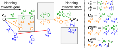
Figure 5: Batch planning in $\mathrm{NeuralPlannerEx}$ algorithm (batch size $B=3$, iteration $i=2$). The algorithm expands three forward paths $\tau_{\mathcal{B}}^{\mathrm{a}}=\left[\tau_{0}^{\mathrm{a}},\tau_{1}^{\mathrm{a}},\tau_{2}^{\mathrm{a}}\right]$ from start $\mathbf{c}_{s}$ towards goal $\mathbf{c}_{g}$ and backward paths $\tau_{\mathcal{B}}^{\mathrm{b}}=\left[\tau_{0}^{\mathrm{b}},\tau_{1}^{\mathrm{b}},\tau_{2}^{\mathrm{b}}\right]$ from $\mathbf{c}_{g}$ towards $\mathbf{c}_{s}$. It computes next waypoints $\mathbf{C}_{\mathcal{B}}^{\mathrm{next}}$ from the current endpoints $\mathbf{C}_{\mathcal{B}}$ using PNet, and then tries to connect forward-backward path pairs for each sample. In the third sample, the endpoint $\mathbf{c}_{2}^{\mathrm{a},1}$ of forward path and a new waypoint $\mathbf{c}_{2}^{\mathrm{b},2}$ of backward path is connectable; it hence concatenates the forward-backward paths ($\tau_{2}^{\mathrm{a}}$, $\tau_{2}^{\mathrm{b}}$) to produce a path from start to goal $\tau=\{\mathbf{c}_{s},\mathbf{c}_{2}^{\mathrm{a},1},\mathbf{c}_{2}^{\mathrm{b},2},\mathbf{c}_{2}^{\mathrm{b},1},\mathbf{c}_{g}\}$.

4.2 Lightweight Encoding and Planning Networks

As depicted in Fig. 3 (right), encoding and planning networks ({E, P}Net) are employed in the MPNet framework to extract features from obstacle point clouds and progressively compute waypoints on the output paths. Instead of {E, P}Net, P3Net uses a lightweight encoder with a PointNet [13] backbone (ENetLite) to extract more robust features, in conjunction with a downsized planning network (PNetLite) for better parameter efficiency and faster inference, which are described in the following subsections.

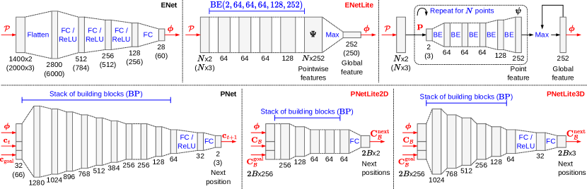
Figure 6: Encoding and planning networks for MPNet and P3Net (top right: sequential feature extraction in Sec. 5.1.1). $\mathrm{BE}$ is a shorthand for a building block consisting of a fully-connected layer, batch normalization, and ReLU activation. $\mathrm{BP}$ is a shorthand for a building block consisting of a fully-connected layer, ReLU activation, and a dropout with a probability of $0.5$.

4.2.1 ENetLite: PointNet-based Encoding Network

As shown in Fig. 6 (top left), MPNet uses a simple encoder architecture (ENet) stacking four FC layers. It directly processes raw point coordinates, and hence costly preprocessing such as normal estimation or clustering is not required. ENet2D takes a point cloud containing 1,400 representative points residing on the obstacles $\mathcal{P}\in\mathbb{R}^{1,400\times 2}$, flattens it into a 2,800D vector, and produces a 28D feature vector $\bm{\phi}(\mathcal{P})\in\mathbb{R}^{28}$ in a single forward pass. Similarly, ENet3D extracts a 60D feature vector $\bm{\phi}(\mathcal{P})$ from a 3D point cloud of size 2,000 with a series of FC layers.

In spite of its simplicity, ENet has the following major drawbacks; (1) the number of input points is fixed to 1,400 or 2,000 regardless of the complexity of planning environments, (2) the number of parameters grows linearly with the number of points, and more importantly, (3) the output feature is affected by the input orderings. This means that ENet produces a different feature if any of the two points are swapped; since the input still represents exactly the same point set, the result should remain unchanged.

P3Net avoids these drawbacks by using PointNet [13] as an encoder backbone, referred to as ENetLite. PointNet is specifically designed for point cloud processing, and Fig. 6 (top center) presents its architecture. It is still a fully-connected network and directly operates on raw point clouds. ENetLite2D first extracts 252D individual features $\left\{\bm{\psi}(\mathbf{p}_{0}),\ldots,\bm{\psi}(\mathbf{p}_{N-1})\right\}$ for each point using a set of blocks represented as $\mathrm{BE}(2,64,64,64,128,252)$. It then computes a 252D global feature $\bm{\phi}(\mathcal{P})=\max\left(\bm{\psi}(\mathbf{p}_{0}),\ldots,\bm{\psi}(\mathbf{p}_{N-1})\right)$ by aggregating these pointwise features via max-pooling. ENetLite3D has the same structure as in the 2D case, except the first and the last building blocks are replaced with $\mathrm{BE}(3,64)$ and $\mathrm{BE}(250)$, respectively, to extract 250D features from 3D point clouds.

Compared to ENet, ENetLite can handle point clouds of any size, and the number of parameters is independent from the input size. ENetLite2D(3D) provides informative features with 9x (28/252) and 4.17x (60/250) more dimensions, while requiring 31.73x (1.60M/0.05M) and 104.47x (5.25M/0.05M) less parameters than ENet2D(3D). PointNet processes each point in a point cloud sequentially and thus avoids random accesses. In addition, as ENetLite involves only pointwise operations and a symmetric pooling function, its output $\bm{\phi}(\mathcal{P})$ is invariant to the permutation of input points, leading to better training efficiency and robustness.

4.2.2 PNetLite: Lightweight Planning Network

The original PNet is formed by a set of building blocks, as shown in Fig. 6 (bottom left). It takes a concatenated input $\left[\bm{\phi}(\mathcal{P}),\mathbf{c}_{t},\mathbf{c}_{\mathrm{goal}}\right]$ consisting of an obstacle feature $\bm{\phi}(\mathcal{P})$ passed from ENet, a current position $\mathbf{c}_{t}$, and a destination $\mathbf{c}_{\mathrm{goal}}$, and computes the next position $\mathbf{c}_{t+1}$ which is one step closer to $\mathbf{c}_{\mathrm{goal}}$. Notably, PNet2D/3D have the same set of hidden layers; the only difference is in the leading and trailing layers. PNet2D uses $\mathrm{BP}(32,1280)$ and $\mathrm{FC}(2)$ to produce 2D coordinates from $28+2\cdot 2=32$D inputs, whereas PNet3D uses $\mathrm{BP}(66,1280)$ and $\mathrm{FC}(3)$ to handle $60+3\cdot 2=66$D inputs and $3$D outputs.

Such design has a problem of low parameter efficiency especially in the 2D case; PNet2D will contain redundant layers which do not contribute to the successful planning and only increase the inference time. The network architecture can be adjusted to the number of state dimensions and the complexity of planning tasks. In addition, as discussed in Sec. 4.2.1, PointNet encoder provides robust (permutation-invariant) features which better represent the planning environment. Assuming that MPNet uses a larger PNet in order to compensate for the lack of robustness and geometric information in ENet-extracted features, it is reasonable to expect that PointNet allows the use of more shallower networks for path planning.

From the above considerations, P3Net employs more compact planning networks with fewer building blocks, PNetLite. PNetLite2D (Fig. 6 (bottom center)) is composed of six building blocks to compute a 2D position from a $252+2\cdot 2=256$D input. As described in Sec. 4.1.1, $\mathrm{NeuralPlannerEx}$ plans $B$ pairs of forward-backward paths and thus the input batch size increases to $2B$; PNetLite computes a batch of next positions $\mathbf{C}_{\mathcal{B}}^{\mathrm{next}}\in\mathbb{R}^{2B\times 2}$ from a matrix $[\bm{\phi}(\mathcal{P}),\mathbf{C}_{\mathcal{B}}^{\mathrm{next}},\mathbf{C}_{\mathcal{B}}^{\mathrm{goal}}]\in\mathbb{R}^{2B\times 256}$. PNetLite3D is obtained by removing a few blocks from PNet3D and replacing the first block with $\mathrm{BP}(256,1024)$ to process $250+3\cdot 2=256$D inputs, as depicted in Fig. 6 (bottom right). PNetLite2D(3D) has 32.58x (3.76M/0.12M) and 2.35x (3.80M/1.62M) less parameters than PNet2D(3D); combining the results from Sec. 4.2.1, {E, P}NetLite together achieves 32.32x (5.43x) parameter reduction in the 2D (3D) case.

5 Implementation

This section details the design and implementation of P3NetCore, a custom IP core for P3Net. It has three submodules, namely, (1) Encoder, (2) NeuralPlanner, and (3) CollisionChecker (Fig. 10), which cover most of the P3Net (Alg. 2) except the evaluation of path costs (lines 18, 22).

5.1 Encoder Module

While the number of parameter is greatly reduced, ENetLite requires a longer inference time than ENet (Table 3 (top)), as it extracts local features for each point, which amounts to $N$ times of forward pass. Encoder module is to accelerate the ENetLite inference (Alg. 2, line 3). To reduce the memory cost from $\mathcal{O}(N)$ to $\mathcal{O}(1)$, it sequentially updates the output feature $\bm{\phi}(\mathcal{P})$. In addition, it applies both coarse and fine-grained optimizations.

5.1.1 Memory-Efficient Sequential Feature Extraction

The typical approach for extracting an ENetLite feature is to first compute individual features $\mathbf{\Psi}=\left\{\bm{\psi}(\mathbf{p}_{0}),\ldots,\bm{\psi}(\mathbf{p}_{N-1})\right\}$ for all points in one shot, creating a matrix of size $(N,252)$ (or $(N,250)$ in the 3D case), and apply max-pooling over $N$ features to produce a 252D (250D) global feature $\bm{\phi}(\mathcal{P})=\max(\mathbf{\Psi})$. In this case, each building block involves a matrix-matrix operation. While it offers a high degree of parallelism and are hardware-amenable, the buffer size for layer outputs is $\mathcal{O}(N)$, which incurs a high utilization of the scarce on-chip memory.

Since the operations for each point is independent except the last max-pooling, instead of following the above approach, the module computes a point feature $\bm{\psi}(\mathbf{p}_{i})$ one-by-one and updates the global feature by taking a maximum $\bm{\phi}(\mathcal{P})\leftarrow\max(\bm{\phi}(\mathcal{P}),\bm{\psi}(\mathbf{p}_{i}))$ (Fig. 6 (top right)). After repeating this process for all $N$ points, the result $\bm{\phi}(\mathcal{P})$ is exactly the same as the previous one, $\max(\mathbf{\Psi})$. In this way, the computation inside each building block turns into a matrix-vector operation. As it only requires an input and output buffer for a single point, the buffer size is reduced from $\mathcal{O}(N)$ to $\mathcal{O}(1)$; Encoder module can now handle point clouds of any size regardless of the limited on-chip memory.

5.1.2 ENetLite Inference

Encoder module consists of three kinds of submodules: $\mathrm{FC}(m,n)$, $\mathrm{BN\text{-}ReLU}(n)$, and $\mathrm{Max}$. $\mathrm{FC}(m,n)$ involves a matrix-vector product $\mathbf{W}^{\top}\mathbf{x}+\mathbf{b}$, and $\mathrm{Max}$ updates the feature by $\max(\bm{\phi}(\mathcal{P}),\bm{\psi})$. $\mathrm{BN\text{-}ReLU}(n)$ couples the batch normalization and ReLU. It is written as $\max(\mathbf{0},(\mathbf{x}-\bm{\mu}_{\mathcal{B}})\cdot\mathbf{s}+\bm{\beta}),\mathbf{s}=\bm{\gamma}/\sqrt{\bm{\sigma}_{\mathcal{B}}^{2}+\varepsilon}\in\mathbb{R}^{n}$ with a little abuse of notations. $\mathrm{FC}(m,n)$ and $\mathrm{BN\text{-}ReLU}(n)$ are parallelized by partially unrolling the loop and partitioning the relevant buffers. Besides, a dataflow optimization is applied for the fully-pipelined execution of these submodules (Fig. 7 (top)). This effectively reduces the latency while requiring a few additional memory resources for inserting pipeline buffers.

5.1.3 Processing Flow of Encoder Module

Fig. 7 (bottom) shows the block diagram of Encoder module. Upon a request from the CPU, it first (1) initializes the output feature $\bm{\phi}(\mathcal{P})$ with zeros. Then, the input $\mathcal{P}$ is processed in fixed-size chunks as follows: the module (2) transfers a chunk from DRAM to a point buffer of size $(N_{C},D)$ ($N_{C}=64,D=2,3$) via burst transfer, and (3) the submodule pipeline consumes points in this buffer one-by-one to update the output. After repeating this process for all $\lceil N/N_{C}\rceil$ chunks, (4) the output $\bm{\phi}(\mathcal{P})$ is written to the on-chip buffer of size $(2B,256)$ for later use in NeuralPlanner module. On-chip buffers for an input chunk, an output $\bm{\phi}$, intermediate outputs, and model parameters are all implemented with BRAM. The lightweight ENetLite model and a sequential update of outputs, which substantially reduce the model parameters and make buffer sizes independent from the number of input points, are essential to place the buffers on BRAM and avoid DRAM accesses during computation.

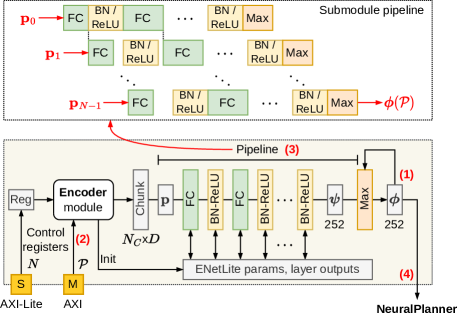
Figure 7: Pipeline of submodules for ENetLite (top) and block diagram of Encoder module (bottom).

5.2 NeuralPlanner Module

As apparent in Algs. 1–2, the bidirectional neural planning ($\mathrm{NeuralPlannerEx}$) is at the core of P3Net and thus has a significant impact on the overall performance. In contrast to the previous work [43], which only offloads the PNet inference (line 11) to the custom IP core, NeuralPlanner module runs the entire $\mathrm{NeuralPlannerEx}$ algorithm (Alg. 3). Considering that it alternates between PNetLite inference and collision checks (lines 13-21), implementing both in one place eliminates the unnecessary CPU-FPGA communication and greatly improves the speed.

5.2.1 PNetLite Inference

For PNetLite inference, the module contains two types of submodules: $\mathrm{FC}(m,n)$ and $\mathrm{Dropout\text{-}ReLU}(p)=\mathrm{ReLU}\to\mathrm{Dropout}(p)$ which fuses ReLU and dropout into a single pipelined loop. $\mathrm{FC}(m,n)$ exploits the fine-grained (data-level) parallelism as described in Sec. 5.1.2. Dropout is the key for the stochastic behavior, and PNet inference is interpreted as a deeply-informed sampling (Sec. 3.2). $\mathrm{Dropout\text{-}ReLU}(p)$ with $p=0.5$ is implemented using a famous Mersenne-Twister (MT) [47]; it first generates 32-bit pseudorandom numbers $\left[r_{bi}\right]\in\mathbb{N}^{2B\times n}$ for a batch input $\mathbf{X}=\left[x_{bi}\right]\in\mathbb{R}^{2B\times n}$, and replaces $x_{bi}$ with zero if $x_{bi}<0$ (ReLU) or $r_{bi}<2^{31}$ (the maximum 32-bit integer multiplied by $p$). Note that in the 3D case, parameters for the first three FC layers are kept on the DRAM due to the limited on-chip memory resources, which necessitates a single sweep (burst transfer) of weight and bias parameters in a forward pass.

5.2.2 Collision Checking

In addition to PNetLite inference, NeuralPlanner module deals with collision checking. It adopts a simple approach based on the discretization [40, 12] to check whether the lines are in collision. The line between $\mathbf{c}^{\mathrm{start}},\mathbf{c}^{\mathrm{end}}$ is divided into segments with a predefined interval $\delta$ (Fig. 8 (right top)), producing equally spaced midpoints $\mathbf{c}_{0},\ldots,\mathbf{c}_{M}$, and then each midpoint $\mathbf{c}_{i}$ is tested. If any midpoint collides with any obstacle, the line is in collision. To simplify the implementation, the module assumes that each obstacle is rectangular and represented as a bounding box with minimum and maximum corner points $\mathbf{c}_{i,\min}^{\mathrm{obs}},\mathbf{c}_{i,\max}^{\mathrm{obs}}$. The module contains eight $\mathrm{Check}$ submodules to test a midpoint $\mathbf{c}_{i}$ with eight obstacles in parallel (Fig. 8 (right bottom)).

5.2.3 Processing Flow of NeuralPlanner Module

As shown in Figs. 8-9, the module interacts with submodules and manages several buffers to perform the bidirectional planning (Alg. 3). To start planning, the module first (1) reads the task configurations such as start-goal points $\mathbf{c}_{s},\mathbf{c}_{g}$ from DRAM, as well as algorithmic parameters (e.g., the number of obstacles $N^{\mathrm{obs}}$, maximum iterations $I$, collision check step $\delta$, etc.) from control registers. It then (2) initializes BRAM buffers (Fig. 9 (top)) for the current endpoints, destinations, next waypoints $\mathbf{C}_{\mathcal{B}},\mathbf{C}_{\mathcal{B}}^{\mathrm{goal}},\mathbf{C}_{\mathcal{B}}^{\mathrm{next}}\in\mathbb{R}^{2B\times D}$ ($D=2,3$) and path lengths $\ell_{\mathcal{B}}\in\mathbb{N}^{2B}$, as well as the result buffers on DRAM (Alg. 3, lines 3-9). These result buffers store the entire forward-backward paths $\tau_{\mathcal{B}}^{\mathrm{a}},\tau_{\mathcal{B}}^{\mathrm{b}}$ along with their lengths and success flags in a format depicted in Fig. 9 (bottom). Its size is bound by the maximum iterations $I$. The on-chip length buffer $\ell_{\mathcal{B}}$ serves as a pointer to the end of path data (Fig. 9, red arrows).

The module proceeds to alternate between PNetLite inference (line 11) and collision checking (lines 13-21); it (3) writes PNetLite inputs $\mathbf{C}_{\mathcal{B}},\mathbf{C}_{\mathcal{B}}^{\mathrm{goal}}$ and computes the next waypoints $\mathbf{C}_{\mathcal{B}}^{\mathrm{next}}$ (Fig. 8 (left bottom)). The buffers for inference are implemented with BRAM or URAM. Using the current and next endpoints ($\mathbf{c}_{j}^{\mathrm{a},i},\mathbf{c}_{j}^{\mathrm{b},i}\in\mathbf{C}_{\mathcal{B}}$, $\mathbf{c}_{j}^{\mathrm{a},i+1},\mathbf{c}_{j}^{\mathrm{b},i+1}\in\mathbf{C}_{\mathcal{B}}^{\mathrm{next}}$), the module (4) attempts to connect each path pair $\tau_{j}^{\mathrm{a}},\tau_{j}^{\mathrm{b}}$ ($j\in\left[1,B\right)$) by the collision checking (Fig. 5). If the path connection succeeds, it transfers the success flag and path length ($\ell_{j}^{\mathrm{a}},\ell_{j}^{\mathrm{b}}\in\ell_{\mathcal{B}}$) to the DRAM result buffer and completes the task. The module appends new waypoints $\mathbf{C}_{\mathcal{B}}^{\mathrm{next}}$ to the DRAM result buffers, increments path lengths $\ell_{\mathcal{B}}$ accordingly, and updates the endpoint buffer $\mathbf{C}_{\mathcal{B}}$ with $\mathbf{C}_{\mathcal{B}}^{\mathrm{next}}$ for the next iteration.

As discussed in Sec. 5.2.2, the collision check of a line segment ($\mathbf{c}^{\mathrm{start}},\mathbf{c}^{\mathrm{end}}$) is cast as checks on the interpolated discrete points $\{\mathbf{c}_{i}\}$. The module reads a chunk of bounding boxes $\{(\mathbf{c}_{i,\min}^{\mathrm{obs}},\mathbf{c}_{i,\max}^{\mathrm{obs}})\}$ into an on-chip obstacle buffer of size $(N_{C}^{\mathrm{obs}},D)$ ($N_{C}^{\mathrm{obs}}=64$), and tests each midpoint $\mathbf{c}_{i}$ with multiple obstacles in parallel using an array of $\mathrm{Check}$ submodules (Fig. 8 (right bottom)).

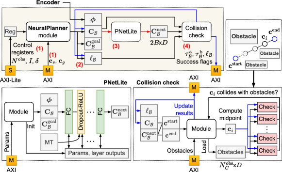
Figure 8: Block diagram of NeuralPlanner module.

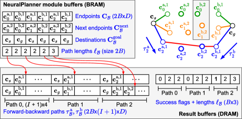
Figure 9: Buffer formats for NeuralPlanner module (batch size $B=3$). NeuralPlanner updates the path endpoints $\mathbf{C}_{\mathcal{B}},\mathbf{C}_{\mathcal{B}}^{\mathrm{next}}$, path lengths $\ell_{\mathcal{B}}$, as well as the DRAM buffers for forward-backward paths $\tau_{\mathcal{B}}^{\mathrm{a}}=\left[\tau_{0}^{\mathrm{a}},\tau_{1}^{\mathrm{a}},\tau_{2}^{\mathrm{a}}\right],\tau_{\mathcal{B}}^{\mathrm{b}}=\left[\tau_{0}^{\mathrm{b}},\tau_{1}^{\mathrm{b}},\tau_{2}^{\mathrm{b}}\right]$ at each iteration. The path lengths stored on-chip are used as pointers to the DRAM path buffers (red arrows). In iteration $i=2$, the third path pair $\tau_{2}^{\mathrm{a}},\tau_{2}^{\mathrm{b}}$ is found to be connectable. The module writes the success flags and path lengths $\ell_{\mathcal{B}}$ to the DRAM buffer and completes the task.

5.3 CollisionChecker Module

Since collision checking is performed throughout P3Net, it is implemented in a dedicated CollisionChecker module for further speedup. It is in charge of testing the path $\tau=\left\{\mathbf{c}_{0},\ldots,\mathbf{c}_{T}\right\}$ by repeating the process described in Sec. 5.2.2 for each edge ($\mathbf{c}_{i},\mathbf{c}_{i+1}$). The path $\tau$ and obstacle bounding boxes $\{(\mathbf{c}_{i,\min}^{\mathrm{obs}},\mathbf{c}_{i,\max}^{\mathrm{obs}})\}$ are stored on the separate DRAM buffers, which are successively transferred to the on-chip buffers of size $(T_{C},D)$ and $(N_{C}^{\mathrm{obs}},D)$ ($T_{C}=64,N_{C}^{\mathrm{obs}}=64$). The module checks the collision between obstacles and interpolated points on the edge $(\mathbf{c}_{i},\mathbf{c}_{i+1})$, and the result (1 if $\tau$ collides with any obstacle) is written to the control register.

5.4 Board-level Implementation of P3NetCore

Fig. 10 shows the board-level implementation for Xilinx Zynq UltraScale+ MPSoC devices. P3NetCore is implemented on the PL (Programmable Logic) part and communicates with the PS (Processing System) part via two AXI interfaces. One is an AXI4-Lite subordinate interface with a 32-bit data bus connected to the High-Performance Master (HPM0) port, which allows PS part to access control registers. The other is an AXI master interface with a 128-bit data bus connected to the High-Performance (HP0) port, through which the IP core transfers algorithm inputs/outputs in bursts (four 32-bit words per clock). We used Xilinx Vitis HLS 2022.1 to develop the IP core, and Vivado 2022.1 for synthesis and place-and-route. Two variants of P3NetCore were created for 2D and 3D planning tasks. The target FPGA SoC is a Xilinx ZCU104 Evaluation Kit (Fig. 11, Table 1). The clock frequency of the board is set to 200MHz.

To preserve the precision of PNetLite outputs (i.e., waypoint coordinates), Encoder and NeuralPlanner modules employ a 32-bit fixed-point with 16.16 format (i.e., a 16-bit integer part and 16-bit fraction part) for layer outputs, and 24-bit fixed-point with 8.16 format for model parameters. Besides, collision checking is performed using the 32-bit floating-point, taking into account that the interval $\delta$ (Sec. 5.2.2) is set sufficiently small to prevent false negatives.

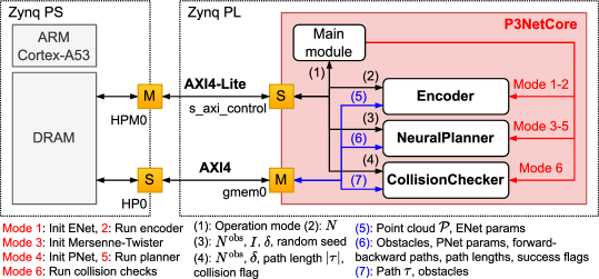
Figure 10: Board-level implementation of P3NetCore.

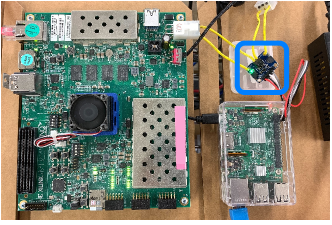
Figure 11: Xilinx ZCU104 Evaluation Kit with Texas Instruments INA219 power monitor (skyblue) and Raspberry Pi 3 Model B (bottom right).

As shown in Fig. 10, P3NetCore has six operation modes, namely, Init{ENet, MT, PNet} and Run{Encoder, Planner, CollisionChecker}. When the IP core is called from the CPU, it first reads an operation mode from the control register and performs the corresponding task. Init{E, P}Net is responsible for transferring the parameters of {E, P}NetLite from DRAM to the dedicated on-chip buffers via an AXI master port. When InitMT is specified, the main module reads a 32-bit random seed from the register and initializes the internal states (624 words) of Mersenne-Twister for dropout layers (Sec. 5.2.1). Run{Encoder, Planner, CollisionChecker} triggers the respective module (Sec. 5.1-5.3). The transferred data is summarized in Fig. 10 (bottom).

6 Evaluation

This section evaluates the proposed P3Net to demonstrate the improvements on success rate, speed, quality of solutions, and power efficiency. For convenience, P3Net accelerated by the proposed IP core is referred to as P3NetFPGA.

6.1 Experimental Setup

MPNet and the famous sampling-based methods, RRT* [8], Informed-RRT* (IRRT*) [10], BIT* [11], and ABIT* [16] were used as a baseline. All methods including P3Net were implemented in Python using NumPy and PyTorch. The implementation of RRT*, Informed-RRT*, and BIT* is based on the open-source code [48]. We implemented an ABIT* planner following the algorithm in the paper [16]. For MPNet, we used the code from the authors [12] as a reference; MPNet path planner and the other necessary codes for training and testing were rewritten from scratch.

The experiments were conducted on a workstation, Nvidia Jetson {Nano, Xavier NX}, and Xilinx ZCU104; their specifications and environments are summarized in Table 1. For ZCU104, we built PyTorch from source with -O3 optimization level and ARM Neon intrinsics enabled (-D__NEON__) to fully take advantage of the multicore architecture.

Following the MPNet paper [12], we trained encoding and planning networks in an end-to-end supervised manner, which is outlined as follows. Given a training sample $(\mathcal{P},\mathbf{c}_{t}^{*},\mathbf{c}^{\mathrm{goal}},\mathbf{c}_{t+1}^{*})$, where $\mathbf{c}_{t}^{*},\mathbf{c}_{t+1}^{*}$ denote a pair of waypoints on a ground-truth path, the encoder first extracts a global feature $\bm{\phi}(\mathcal{P})$, and then the planning network estimates the next waypoint $\mathbf{c}_{t+1}$. The squared Euclidean distance $\|\mathbf{c}_{t+1}-\mathbf{c}_{t+1}^{*}\|^{2}$ is used as a loss function, so that two models jointly learn to mimic the behavior of the planner used for dataset generation. We used an Adam optimizer with a learning rate of $10^{-3}$ and coefficients of $\beta_{1}=0.9,\beta_{2}=0.999$. We set the number of epochs to 200 and 50 when training MPNet and P3Net, and the batch size to 8192 for MPNet (2D), 1024 for MPNet (3D), and 128 for P3Net models, respectively. The number of iterations $I$ in $\mathrm{NeuralPlanner}$($\mathrm{Ex}$) (Algs. 1, 3) is fixed to 50.

RRT* and Informed-RRT* were configured with a maximum step size of 1.0 and a goal bias of $0.05$. BIT* and ABIT* were executed with a batch size of 100 and Euclidean distance heuristic. As done in [16], ABIT* searched the same batch twice with two different inflation factors $\varepsilon_{\mathrm{infl}}=10^{6},1+\frac{10}{q}$, and the truncation factor $\varepsilon_{\mathrm{trunc}}$ was set to $1+\frac{5}{q}$, where $q$ is a total number of nodes.

Table 1: Evaluation Environments

	Workstation	Nvidia Jetson Nano
CPU	Intel Xeon W-2235	ARM Cortex-A57
	@3.8GHz, 12C	@1.43GHz, 4C
GPU	Nvidia GeForce RTX 3090	128-core Nvidia Maxwell
DRAM	64GB (DDR4)	4GB (DDR4)
OS	Ubuntu 20.04.6	Nvidia JetPack 4.6.3
		(based on Ubuntu 18.04)
Python	3.8.2	3.6.15
PyTorch	1.11.0 (w/ CUDA 11.3)	1.10.0 (w/ CUDA 10.2)
	Nvidia Jetson Xavier NX	Xilinx ZCU104 Evaluation Kit
CPU	Nvidia Carmel ARM v8.2	ARM Cortex-A53
	@1.4GHz, 6C	@1.2GHz, 4C
GPU	384-core Nvidia Volta	–
FPGA	–	XCZU7EV-2FFVC1156
DRAM	8GB (DDR4)	2GB (DDR3)
OS	Nvidia JetPack 5.1	Pynq Linux v2.7
	(based on Ubuntu 20.04)	(based on Ubuntu 20.04)
Python	3.8.2	3.8.2
PyTorch	1.14.0a0 (w/ CUDA 11.4)	1.10.2

6.2 Path Planning Datasets

For evaluation, we used a publicly-available dataset for 2D/3D path planning provided by the MPNet authors [12], referred to as MPNet2D/3D. It is split into one training and two testing sets (Seen, Unseen); the former contains 100 workspaces, each of which has a point cloud $\mathcal{P}$ representing obstacles, and 4000 planning tasks with randomly generated start-goal points and their respective ground-truth paths. Seen set contains the same 100 workspaces as the training set, but with each having 200 new planning tasks; Unseen set comes with ten new workspaces not observed during training, each of which has 2000 planning tasks.

Each workspace is a square (or cube) of size 40 containing randomly-placed seven square obstacles of size 5 (or ten cuboid obstacles with a side length of 5 and 10). Note that, trivial tasks in the testing sets are excluded, where start-goal pairs can be connected by straight lines and obstacle avoidance is not required. We only used the first 20/200 tasks for each workspace in Seen/Unseen dataset. As a result, the total number of planning tasks is 945/892 and 740/756 in MPNet2D (Seen/Unseen) and MPNet3D (Seen/Unseen) datasets, respectively. Both MPNet and P3Net models were trained with MPNet2D/3D training sets.

In addition, we generated P3Net2D/3D dataset for testing (Figs. 2-2), which contains 100 workspaces, with 20 planning tasks for each. Compared to MPNet2D/3D, the number of obstacles is doubled to simulate more challenging tasks.

6.3 Planning Success Rate

First, the tradeoff between planning success rate and the average computation time per task is evaluated on the workstation with GPU acceleration.

6.3.1 Comparison of Encoding and Planning Networks

MPNet is executed under three combinations of models, i.e., {E, P}Net (original), ENetLite-PNet (ELite), and {E, P}NetLite (EPLite), with a varying number of replan iterations $I_{\mathrm{Replan}}=\{10,20,50,100\}$. For P3Net, the refinement step is not performed ($I_{\mathrm{Refine}}=0$). The results on MPNet and P3Net test datasets are shown in Fig. 12 (left).

In the 2D case (1st/3rd row), replacing {E, P}Net with {E, P}NetLite yields substantially higher success rate and even faster computation time, while reducing the parameters by 32.32x (Sec. 4.2.2). For $I_{\mathrm{Replan}}=10$, MPNet with ELite setting is 15.58% (69.17/84.75%) and 23.75% (45.15/68.90%) more successful than the original setting on MPNet (Unseen) and P3Net datasets, respectively; PNetLite further improves the success rate by 3.48% (84.75/88.23%) and 4.45% (68.90/73.35%). MPNet (EPLite) is 1.40x (0.067/0.048s) and 1.12x (0.131/0.117s) faster than MPNet (original), indicating that the proposed models help MPNet algorithm to quickly find a solution in a less number of replan attempts. This empirically validates the discussion in Sec. 4.2.1 that the shallower PNet is sufficient since the PointNet encoder produces more robust and informative features. Considering the success rate improvements (19.06/28.20%) in these two datasets, the proposed models offer greater performance advantages in more difficult problem settings.

In the 3D case (Fig. 12 (2nd/4th row, left)), MPNet (EPLite) maintains the same level of performance as MPNet (original), while achieving 5.43x parameter reduction (Sec. 4.2.2). ENetLite improves the success rate by 1.46% (89.82/91.27%) and 3.70% (79.35/83.05%), whereas PNetLite slightly lowers it by 0.40% (91.27/90.87%) and 3.95% (83.05/79.10%) on MPNet (Unseen) and P3Net datasets. This performance loss is compensated by the P3Net planner. Comparing the results from MPNet Seen/Unseen datasets (dashed/solid lines), the difference in the success rate is at most 3.46%, which confirms that our proposed models generalize to workspaces that are not observed during training.

6.3.2 Comparison of P3Net with MPNet

Fig. 12 (left) also highlights the advantage of P3Net ($B=\{1,2,4,8\},I_{\mathrm{Replan}}=\{10,20,50,100\}$). Though MPNet exhibits gradual improvement in success rate with increasing $I_{\mathrm{Replan}}$, P3Net consistently outperforms MPNet and achieves nearly 100% success rate. In the 2D case (1st/3rd row), P3Net ($B,I_{\mathrm{Replan}}=8,100$) is 2.80% (96.30/99.10%) and 9.85% (87.60/97.45%) more likely to find a solution in 2.20x (0.101/0.046s) and 1.55x (0.326/0.210s) shorter time than MPNet (EPLite, $I_{\mathrm{Replan}}=100$) on MPNet (Unseen) and P3Net datasets. While MPNet shows a noticeable drop in success rate (96.30/87.69%) when tested on P3Net dataset, P3Net only shows a 1.65% drop (99.10/97.45%) and maintains the high success rate in a more challenging dataset. In the 3D case (2nd/4th row), it is 2.91% (96.69/99.60%) and 8.00% (91.75/99.75%) better while spending 2.70x (0.081/0.030s) and 1.02x (0.277/0.272s) less time.

Notably, increasing the batch size $B$ improves both success rate and speed, which clearly indicates the effectiveness of the batch planning strategy (Sec. 4.1.1). On P3Net2D dataset (3rd row), P3Net with $B,I_{\mathrm{Replan}}=8,10$ is 5.25% more successful and 1.88x faster than with $B=1$ (79.40/84.65%, 0.128/0.068s). The number of initial planning attempts $I_{\mathrm{Init}}$ also affects the performance; increasing it from 1 to 5 yields a 2.85% better success rate on P3Net2D dataset ($I_{\mathrm{Replan}}=10$). Table 2 compares the success rate of P3NetFPGA and P3Net; despite the use of fixed-point arithmetic and a simple pseudorandom generator, P3NetFPGA attains a similar performance.

6.3.3 Comparison with Sampling-based Methods

Fig. 12 (right) plots the results from sampling-based methods. The number of iterations is set to $\{200,300,400,500\}$ for RRT*/IRRT*, and $\{50,100,200\}$ for BIT*/ABIT*. As expected, sampling-based methods exhibit a higher success rate with increasing iterations; they are more likely to find a solution as they place more random nodes inside a workspace and build a denser tree. P3Net achieves a success rate comparable to ABIT*, and outperforms the other methods. On P3Net2D dataset, P3Net ($B,I_{\mathrm{Replan}}=8,100$) plans a path in an average of 0.214s with 97.60% success rate, which is 1.84/5.69x faster and 0.95/2.20% better than ABIT*/BIT* (200 iterations).

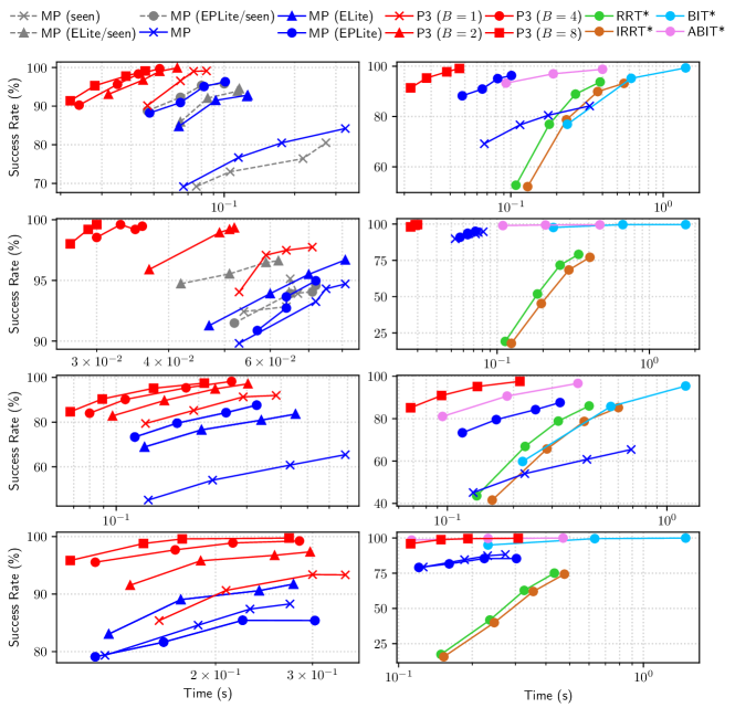
Figure 12: Success rate and computation time tradeoffs (MPNet{2D, 3D}, P3Net{2D, 3D} dataset from top to bottom, measured on the workstation with GPU acceleration). Upper left is better.

Table 2: Success rate of P3NetFPGA and P3Net (w/ and w/o P3NetCore)

MPNet (2D) dataset				MPNet (3D) dataset
$B$	$I_{\mathrm{Replan}}$	% (w/)	% (w/o)	$B$	$I_{\mathrm{Replan}}$	% (w/)	% (w/o)
4	10	91.70	91.26	4	10	97.88	97.88
4	20	95.18	94.84	4	20	99.07	99.47
4	50	98.54	98.54	4	50	99.60	99.60
4	100	99.78	99.66	4	100	99.60	99.60
P3Net (2D) dataset				P3Net (3D) dataset
$B$	$I_{\mathrm{Replan}}$	% (w/)	% (w/o)	$B$	$I_{\mathrm{Replan}}$	% (w/)	% (w/o)
4	10	84.75	84.25	4	10	94.95	95.60
4	20	91.40	91.00	4	20	98.90	98.90
4	50	95.45	95.45	4	50	99.60	99.75
4	100	98.25	97.80	4	100	99.80	100.0

6.4 Computation Time

Fig. 13 visualizes the distribution of computation time measured on the workstation and SoC devices (Table 1). The sampling-based methods were run on the CPU. On Nvidia Jetson, MPNet and P3Net were executed with GPU. WS {CPU, GPU} refers to the workstation with and without GPU acceleration. On the basis of results from Sec. 6.3, hyperparameters of the planners were selected to achieve similar success rates. For a fair comparison, the PS–PL data transfer overhead is included in P3NetFPGA.

As expected, P3NetFPGA is faster than the other planners on ZCU104 and Jetson (green, brown, skyblue) in most cases, and its median computation time is below 0.1s. In the 2D case (Fig. 13 (left)), it even outperforms sampling-based methods on the WS CPU (pink), and is comparable to MPNet/P3Net on the WS GPU (orange). On P3Net2D dataset, P3NetFPGA takes 0.062s in the median to solve a task, which is 2.15x, 1.13x, 6.11x, and 17.52x faster than P3Net (GPU), MPNet (GPU), ABIT*, and BIT* on the workstation. P3Net offers more performance advantages in a more challenging dataset. On the ZCU104 and P3Net/MPNet2D dataset, P3NetFPGA is 15.57x/9.17x faster than MPNet (CPU).

In the 3D case (Fig. 13 (right)), while MPNet on the workstation looks faster than P3NetFPGA, it only solves easy planning tasks which require less replan trials, and the result shows around 10% lower success rate. We observe a significant reduction of the variance in computation time. On the ZCU104 and P3Net dataset (Fig. 13, bottom right), P3Net solves a task in 7.623$\pm$19.987s on average, which is improved to 4.651$\pm$8.909s and 0.145$\pm$0.170s in P3Net (CPU, FPGA). As seen from the results of WS {CPU, GPU}, GPU acceleration of the DNN inference does not contribute to the overall performance improvement; since MPNet/P3Net alternates between collision checks (CPU) and PNet inference (GPU), the frequent CPU–GPU data transfer undermines the performance gain obtained by GPU.

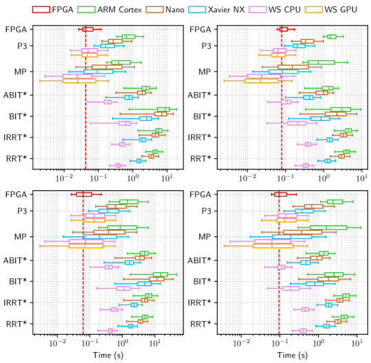
Figure 13: Computation time distribution (top: MPNet, bottom: P3Net dataset, left: 2D, right: 3D dataset). Hyperparameters are as follows. P3Net2D: $(B,I_{\mathrm{Init}},I_{\mathrm{Replan}},I_{\mathrm{Refine}})=(4,5,50,5)$, P3Net3D: $(B,I_{\mathrm{Init}},I_{\mathrm{Replan}},I_{\mathrm{Refine}})=(4,5,20,5)$, MPNet2D/3D: {E, P}NetLite, $I_{\mathrm{Replan}}=100$, ABIT*/BIT* (2D): 100/200 iterations for MPNet/P3Net dataset, ABIT*/BIT* (3D): 50 iterations, IRRT*/RRT* (2D/3D): 500 iterations. The red dashed line is a median time of P3NetFPGA.

6.4.1 Path Planning Speedup

Fig. 14 shows the performance gain of P3NetFPGA over the other planners on the workstation and SoC devices. In the 2D case, P3NetFPGA is the fastest among the methods considered. On P3Net dataset (bottom left), it achieves 24.54–149.57x, 10.74–115.25x, 6.19–47.36x, and 2.34–10.76x speedups over the ZCU104, Jetson Nano, Jetson Xavier NX, and a workstation, respectively. Offloading the entire planning algorithm (collision checks and neural planning in Alg. 3) to the dedicated IP core eliminates unnecessary data transfers and brings more performance benefits than highend CPUs. In this evaluation, we compared the sum of execution times for successful planning tasks to compute average speedup factors. Unlike MPNet, P3Net also performs an extra refinement phase ($I_{\mathrm{Refine}}=5$). This means P3NetFPGA completes more planning tasks in a shorter period of time than MPNet (e.g., 7.85% higher success rate and 2.92x speedup than MPNet (WS GPU)). Additionally, while P3NetFPGA shows a 1.13x speedup over P3Net (WS GPU) in terms of median time (Fig. 13 (bottom left)), the total execution time is reduced by 2.92x (Fig. 14 (bottom left)). This implies P3Net solves challenging tasks much faster than MPNet, which is attributed to the improved algorithm and model architecture. Also in the 3D case, P3NetFPGA outperforms the other planners except a few cases. On P3Net3D dataset (Fig. 14 (bottom right)), it provides 10.03–59.47x, 6.69–28.76x, 3.38–14.62x, and 0.79–3.65x speedups compared to the ZCU104, Jetson Nano, Jetson Xavier NX, and a workstation, respectively.

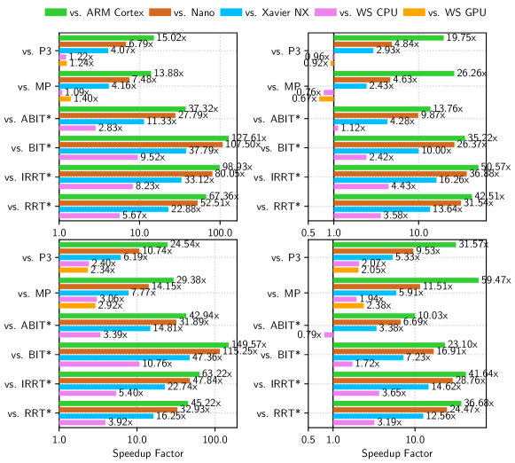
Figure 14: Average speedup factors (top: MPNet, bottom: P3Net, left: 2D, right: 3D dataset). Hyperparameter settings are the same as in Fig. 13.

6.4.2 Computation Time Breakdown

The computation time breakdown of MPNet/P3Net is summarized in Fig. 15. P3NetCore effectively reduces the execution time of all three phases. On P3Net2D dataset (bottom left), the replanning phase (pink) took 3.041s and accounted for 89.24% of the entire execution time in MPNet, which is almost halved to 1.557s (51.37%) in P3Net (CPU), and is brought down to only 0.062s (51.46%) in P3NetFPGA. The saved time can be used to perform the additional refinement step (orange) and improve the quality of solutions.

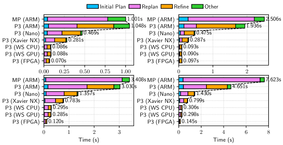
Figure 15: Computation time breakdown of P3NetFPGA in comparison with MPNet and P3Net (top: MPNet, bottom: P3Net, left: 2D, right: 3D dataset). Hyperparameter settings are the same as in Fig. 13.

6.4.3 Speedup of Inference and Collision Checking

Table 3 (top) lists the inference time of {E, P}Net and {E, P}NetLite, measured on the ZCU104 with and without the P3NetCore. The data is the average of 50 runs. As mentioned in Sec. 5.1, ENetLite basically involves $N$ times of forward passes to compute pointwise features, which increases the inference time by 3.78/1.57x than ENet2D/3D ($N=1400,2000$). P3NetCore accelerates the inference by 45.47/45.34x and as a result achieves 12.01/28.88x faster feature extraction than ENet. P3NetCore consistently attains around a 45x speedup on a wide range of $N$, owing to the combination of inter-layer pipelining (Fig. 7 (top)) and parallelization within each layer. The inference time increases proportionally to $N$, which corresponds to the $\mathcal{O}(N)$ complexity of ENetLite, and P3NetCore yields a better performance gain with a larger $N$ (e.g., 45.47/47.13x in $N=1400,4096$, 2D).

PNetLite has a 28.87/2.32x shorter inference time than PNet2D/3D, mainly due to the 32.58/2.35x parameter reduction (Sec. 4.2.2). It does not grow linearly with the batch size $B$, indicating that the batch planning strategy in P3Net effectively improves success rates without incurring a significant additional overhead. With P3NetCore, PNetLite is sped up by 10.15–11.49/16.55–17.44x, resulting in an overall speedup of 280.45–326.25/38.27–40.48x over PNet.

Table 3 (bottom) presents the computation time of collision checking on the ARM Cortex CPU and P3NetCore. We conducted experiments with four random workspaces of size 40 containing different numbers of obstacles $N^{\mathrm{obs}}$, and 50 random start-goal pairs with a fixed distance of $d=5.0,20.0$ for each workspace. The interval $\delta$ is set to 0.01. P3NetCore gives a larger speedup with the increased problem complexity (larger $d$ or $N^{\mathrm{obs}}$). It runs 2D/3D collision checking 10.49–55.19/31.92–221.45x (11.34–60.56/30.82–181.12x) faster in case of $d=5.0$ and $20.0$, respectively. The parallelization with an array of pipelined submodules (Sec. 5.1.3) contributes to the two orders of magnitude performance improvement. The result from P3NetCore does not show a linear increase with $N^{\mathrm{obs}}$, as P3NetCore terminates the checks as soon as any of midpoints between start-goal points is found to be in collision, and such early-exit is more likely to occur in a cluttered workspace with more obstacles. A slight latency jump at $N^{\mathrm{obs}}=128$ is due to the limited buffer size for obstacle positions and the increased data transfer from DRAM.

Table 3: Latency for inference (top) and collision checking (bottom) on Xilinx ZCU104

	2D			3D
Model	$N$	CPU (ms)	IP (ms)	$N$	CPU (ms)	IP (ms)
ENet	1400	43.25	–	2000	146.40	–
ENetLite	1400	163.70	3.60	2000	229.85	5.07
	2048	242.05	5.18	4096	478.06	10.15
	4096	477.47	10.13	8192	950.91	20.11
Model	$B$	CPU (ms)	IP (ms)	$B$	CPU (ms)	IP (ms)
PNet	1	102.77	–	1	103.22	–
	2	107.79	–	2	108.31	–
	4	130.41	–	4	130.68	–
PNetLite	1	3.56	0.315	1	44.48	2.55
	2	4.02	0.350	2	46.85	2.83
	4	4.72	0.465	4	56.63	3.38
	2D			3D
Dist.	$N^{\mathrm{obs}}$	CPU (ms)	IP (ms)	$N^{\mathrm{obs}}$	CPU (ms)	IP (ms)
5.0	16	3.02	0.288	16	3.29	0.290
	32	5.23	0.290	32	5.75	0.291
	64	9.65	0.284	64	10.68	0.291
	128	18.49	0.335	128	20.59	0.340
20.0	16	10.12	0.317	16	11.22	0.364
	32	18.97	0.300	32	21.18	0.380
	64	36.91	0.301	64	41.09	0.386
	128	72.86	0.329	128	80.78	0.446

6.5 Path Cost

This subsection evaluates the quality of solutions returned from P3Net in comparison with the other planners. The relative path cost is used as a quality measure; it is computed by dividing a length of the output path by that of the ground-truth available in the dataset. Fig. 16 shows the results on the MPNet/P3Net datasets ($I_{\mathrm{Refine}}$ is set to 5).

P3Net (skyblue) produces close-to-optimal solutions and an additional refinement step further improves the quality of outputs (red). On P3Net2D dataset, P3Net with/without refinement achieves the median cost of 1.001/1.026, which is comparable to the sampling-based methods (1.038, 1.012, 1.174, and 1.210 in ABIT*, BIT*, IRRT*, and RRT*). If we apply smoothing and remove unnecessary waypoints from the solutions in these sampling-based methods, the median cost reduces to 1.036, 1.011, 0.996, and 1.000, respectively; while IRRT* and RRT* seem to provide better quality solutions, their success rates (85.35/86.00%) are lower than P3Net (95.45%). These results confirm that PNetLite samples waypoints that are in close proximity to the optimal path, and helps the algorithm to quickly find a solution by creating only a few waypoints.

Fig. 17 plots the path costs over time on the three planning tasks taken from P3Net2D dataset. We run P3Net and IRRT* for 100 seconds and recorded the evolution of path costs to verify the effectiveness of the refinement step. P3NetFPGA (red) finds an initial solution within 0.1s and reaches a close-to-optimal solution within 1.0s, unlike IRRT* (skyblue) that still does not converge after 100s. Figs. 2-2 show examples of the output paths obtained from MPNet and P3NetFPGA on the P3Net dataset.

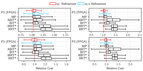
Figure 16: Distribution of the relative path cost (top: MPNet, bottom: P3Net, left: 2D, right: 3D dataset).

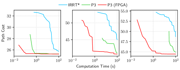
Figure 17: Evolution of the cost on P3Net2D dataset.

6.6 FPGA Resource Consumption

Table 4 summarizes the FPGA resource consumption of P3NetCore ($B=4$). The BRAM consumption is mainly due to the buffers for model parameters and layer outputs. In the 2D case, {E, P}NetLite fits within the BRAM thanks to the parameter reduction and memory-efficient sequential feature extraction (Sec. 5.1.1), which minimizes the memory access latency and brings two orders of magnitude speedup as seen in Table 3 (top left). Since the original {E, P}Net has 32.32x more parameters, they should be stored on the external memory, which would limit the performance gain. While P3NetCore is a package of the three modules with a collision checker and two DNNs, it consumes less than 30% of the onboard DSP, FF, and LUT resources available in both 2D/3D cases. These results demonstrate the resource efficiency of P3NetCore. The batch size $B$ could be set larger (e.g., 8) for further performance (Fig. 12).

Table 4: FPGA resource consumption of P3NetCore ($B=4$)

		BRAM	URAM	DSP	FF	LUT
	Total	312	96	1728	460800	230400
2D	Use	275	–	462	38656	57404
	%	88.14	–	26.74	8.39	24.91
3D	Use	264	42	484	50653	69410
	%	84.62	43.75	28.01	10.99	30.13

6.7 Power Efficiency

Finally, we compare the power consumption of P3NetFPGA with that of P3Net and ABIT*. tegrastats is used to measure the power of Nvidia Jetson. For the workstation, we used s-tui [50] and nvidia-smi to record the power consumption of Intel Xeon W-2235 and Nvidia GeForce RTX 3090. As shown in Fig. 11, we measured the power of the entire ZCU104 board using a Texas Instruments INA219 power monitor (skyblue). We run each planner with P3Net2D/3D datasets for five minutes and averaged the power consumption. To exclude the power consumption of peripherals (e.g., switches and LEDs on the ZCU104), we subtracted the average power consumption in the idle state. Table 5 presents the results.

In the 2D (3D) case, P3NetFPGA consumes 124.51x, 147.80x, and 448.47x (39.64x, 45.60x, and 145.48x) less power than ABIT*, P3Net (CPU), and P3Net (GPU) on the workstation. It also achieves 4.40–5.38/4.58–6.10x (1.36–1.77/1.55–2.07x) power savings over ABIT*/P3Net on Nvidia Jetson. While P3NetFPGA consumes slightly more power than P3Net in the 3D case, this indicates that the power consumption of the P3NetCore itself is at most 0.318W ($0.809-0.491$). Combined with the results from Fig. 14 (bottom), P3NetFPGA offers 65.22–171.71/28.35–65.54x (5.80–17.50/4.53–19.77x) power efficiency than ABIT*/P3Net on ARM Cortex and Nvidia Jetson in the 2D (3D) case. The power efficiency reaches 422.09x, 354.73x, and 1049.42x (44.40x, 43.78x, and 133.84x) when compared with ABIT*, P3Net (CPU), and P3Net (GPU) on the workstation.

Table 5: Comparison of the power consumption (W)

	2D				3D
Machine	ABIT*	P3Net			ABIT*	P3Net
	CPU	CPU	+GPU	+IP	CPU	CPU	+GPU	+IP
ZCU104	0.480	0.461	–	0.255	0.480	0.491	–	0.809
Nano	1.373	–	1.556	–	1.434	–	1.678	–
Xavier	1.123	–	1.168	–	1.097	–	1.250	–
WS	31.75	37.69	114.36*	–	32.07	36.89	117.69*	–

• 114.36W: 29.72 + 84.64 (CPU/GPU); 117.69W: 32.51 + 85.17 (CPU/GPU)

7 Conclusion

In this paper, we have presented a new learning-based path planning method, P3Net. P3Net aims to address the limitations of the recently-proposed MPNet by introducing two algorithmic improvements: it (1) plans multiple paths in parallel for computational efficiency and higher success rate, and (2) iteratively refines the solution. In addition, P3Net (3) employs hardware-amenable lightweight DNNs with 32.32/5.43x less parameters to extract robust features and sample waypoints from a promising region. We designed P3NetCore, a custom IP core incorporating neural path planning and collision checking, to realize a planner on a resource-limited edge device that finds a path in $\sim$0.1s while consuming $\sim$1W. P3NetCore was implemented on the Xilinx ZCU104 board and integrated to P3Net.

Evaluation results successfully demonstrated that P3Net achieves a significantly better tradeoff between computational cost and success rate than MPNet and the state-of-the-art sampling-based methods. In the 2D (3D) case, P3NetFPGA obtained 24.54–149.57x and 6.19–115.25x (10.03–59.47x and 3.38–28.76x) average speedups over ARM Cortex and Nvidia Jetson, respectively, and its performance was even comparable to the workstation. P3NetFPGA was 28.35–1049.42x and 65.22–422.09x (4.53–133.84x and 5.80–44.40x) more power efficient than P3Net and ABIT* on the Nvidia Jetson and workstation, showcasing that FPGA SoC is a promising solution for the efficient path planning. We also confirmed that P3Net converges fast to the close-to-optimal solution in most cases.

P3Net is currently evaluated on the simulated static 2D/3D environments, and the robot is modeled as a point-mass. As a future work, we plan to extend P3Net to more complex settings, e.g., multi-robot problems, dynamic environments, and higher state dimensions. P3NetCore employs a standard fixed-point format for DNN inference; while it already provides satisfactory performance improvements, low-precision formats and model compression techniques (e.g., pruning, low-rank factorization) could be used to further improve the resource efficiency and speed.

References

- [1] Jeonghyeon Pak, Jeongeun Kim, Yonghyun Park, and Hyoung Il Son. Field Evaluation of Path-Planning Algorithms for Autonomous Mobile Robot in Smart Farms. IEEE Access, 10(1):60253–60266, June 2022.
- [2] Hyeonbeom Lee, Hyoin Kim, and H. Jin Kim. Planning and Control for Collision-Free Cooperative Aerial Transportation. IEEE Transactions on Automation Science and Engineering, 15(1):189–201, January 2018.
- [3] Tung Dang, Frank Mascarich, Shehryar Khattak, Christos Papachristos, and Kostas Alexis. Graph-based Path Planning for Autonomous Robotic Exploration in Subterranean Environments. In Proceedings of the IEEE/RSJ International Conference on Intelligent Robots and Systems (IROS), pages 3105–3112, November 2019.
- [4] Francis Colas, Srivatsa Mahesh, François Pomerleau, Ming Liu, and Roland Siegwart. 3D Path Planning and Execution for Search and Rescue Ground Robots. In Proceedings of the IEEE/RSJ International Conference on Intelligent Robots and Systems (IROS), pages 722–727, November 2013.
- [5] Runze Liu, Jianlei Yang, Yiran Chen, and Weisheng Zhao. eSLAM: An Energy-Efficient Accelerator for Real-Time ORB-SLAM on FPGA Platform. In Proceedings of the Annual Design Automation Conference (DAC), pages 1–6, June 2019.
- [6] Pengfei Gu, Ziyang Meng, and Pengkun Zhou. Real-Time Visual Inertial Odometry with a Resource-Efficient Harris Corner Detection Accelerator on FPGA Platform. In Proceedings of the IEEE/RSJ International Conference on Intelligent Robots and Systems (IROS), pages 10542–10548, October 2022.
- [7] Steven M. LaValle. Rapidly-Exploring Random Trees: A New Tool for Path Planning. Technical report, Iowa State University, Technical Report No. 98–11, October 1998.
- [8] Sertac Karaman and Emilio Frazzoli. Sampling-Based Algorithms for Optimal Motion Planning. International Journal of Robotics Research, 30(7):846–894, June 2011.
- [9] Peter E. Hart, Nils J. Nilsson, and Bertram Raphael. A Formal Basis for the Heuristic Determination of Minimum Cost Paths. IEEE Transactions on Systems Science and Cybernetics, 4(2):100–107, July 1968.
- [10] Jonathan D. Gammell, Siddhartha S. Srinivasa, and Timothy D. Barfoot. Informed RRT*: Optimal Sampling-based Path Planning Focused via Direct Sampling of an Admissible Ellipsoidal Heuristic. In Proceedings of the IEEE/RSJ International Conference on Intelligent Robots and Systems (IROS), pages 2997–3004, September 2014.
- [11] Jonathan D. Gammell, Siddhartha S. Srinivasa, and Timothy D. Barfoot. Batch Informed Trees (BIT*): Sampling-based Optimal Planning via the Heuristically Guided Search of Implicit Random Geometric Graphs. In Proceedings of the IEEE International Conference on Robotics and Automation (ICRA), pages 3067–3074, May 2015.
- [12] Ahmed Hussain Qureshi, Yinglong Miao, Anthony Simeonov, and Michael C. Yip. Motion Planning Networks: Bridging the Gap Between Learning-Based and Classical Motion Planners. IEEE Transactions on Robotics, 37(1):48–66, February 2021.
- [13] Charles R. Qi, Hao Su, Kaichun Mo, and Leonidas J. Guibas. PointNet: Deep Learning on Point Sets for 3D Classification and Segmentation. In Proceedings of the IEEE Conference on Computer Vision and Pattern Recognition (CVPR), pages 652–660, July 2017.
- [14] Xu Ma, Can Qin, Haoxuan You, Haoxi Ran, and Yun Fu. Rethinking Network Design and Local Geometry in Point Cloud: A Simple Residual MLP Framework. arXiv preprint arXiv:2202.07123, February 2022.
- [15] Weiyue Wang, Ronald Yu, Qiangui Huang, and Ulrich Neumann. SGPN: Similarity Group Proposal Network for 3D Point Cloud Instance Segmentation. In Proceedings of the IEEE Conference on Computer Vision and Pattern Recognition (CVPR), pages 2569–2678, June 2018.
- [16] Marlin P. Strub and Jonathan D. Gammell. Advanced BIT* (ABIT*): Sampling-Based Planning with Advanced Graph-Search Techniques. In Proceedings of the IEEE International Conference on Robotics and Automation (ICRA), pages 130–136, May 2020.
- [17] Marlin P. Strub and Jonathan D. Gammell. Adaptively Informed Trees (AIT*): Fast Asymptotically Optimal Path Planning through Adaptive Heuristics. In Proceedings of the IEEE International Conference on Robotics and Automation (ICRA), pages 3191–3198, May 2020.
- [18] Brian Ichter, James Harrison, and Marco Pavone. Learning Sampling Distributions for Robot Motion Planning. In Proceedings of the IEEE International Conference on Robotics and Automation (ICRA), pages 7087–7094, May 2018.
- [19] Brian Ichter and Marco Pavone. Robot Motion Planning in Learned Latent Spaces. IEEE Robotics and Automation Letters, 4(3):2407–2414, July 2019.
- [20] Jiankun Wang, Wenzheng Chi, Chenming Li, Chaoqun Wang, and Max Q.-H. Meng. Neural RRT*: Learning-Based Optimal Path Planning. IEEE Transactions on Automation Sciences and Engineering, 17(4):1748–1758, October 2020.
- [21] Ryo Yonetani, Tatsunori Taniai, Mohammadamin Barekatain, Mai Nishimura, and Asako Kanezaki. Path Planning using Neural A* Search. In Proceedings of the International Conference on Machine Learning (ICML), pages 12029–12039, July 2021.
- [22] Alexandru-Iosif Toma, Hussein Ali Jaafar, Hao-Ya Hsueh, Stephen James, Daniel Lenton, Ronald Clark, and Sajad Saeedi. Waypoint Planning Networks. In Proceedings of the IEEE Conference on Robotics and Vision (CRV), pages 87–94, May 2021.
- [23] Masaya Inoue, Takahiro Yamashita, and Takeshi Nishida. Robot Path Planning by LSTM Network Under Changing Environment. In Advances in Computer Communication and Computational Sciences, pages 317–329, August 2018.
- [24] Mayur J. Bency, Ahmed H. Qureshi, and Michael C. Yip. Neural Path Planning: Fixed Time, Near-Optimal Path Generation via Oracle Imitation. In Proceedings of the IEEE/RSJ International Conference on Intelligent Robots and Systems (IROS), pages 3965–3972, November 2019.
- [25] Mark Pfeiffer, Michael Schaeuble, Juan Nieto, Roland Siegwart, and Cesar Cadena. From Perception to Decision: A Data-driven Approach to End-to-end Motion Planning for Autonomous Ground Robots. In Proceedings of the IEEE International Conference on Robotics and Automation (ICRA), pages 1527–1533, June 2017.
- [26] Jinwook Huh, Volkan Isler, and Daniel D. Lee. Cost-to-Go Function Generating Networks for High-Dimensional Motion Planning. In Proceedings of the IEEE International Conference on Robotics and Automation (ICRA), pages 8480–8486, May 2021.
- [27] Adam Fishman, Adithyavairavan Murali, Clemens Eppner, Bryan Peele, Byron Boots, and Dieter Fox. Motion Policy Networks. In Proceedings of the Conference on Robot Learning (CoRL), pages 967–977, November 2022.
- [28] Devendra Singh Chaplot, Deepak Pathak, and Jitendra Malik. Differentiable Spatial Planning using Transformers. In Proceedings of the International Conference on Machine Learning (ICML), pages 1484–1495, July 2021.
- [29] Jacob J. Johnson, Uday S. Kalra, Ankit Bhatia, Linjun Li, Ahmed H. Qureshi, and Michael C. Yip. Motion Planning Transformers: A Motion Planning Framework for Mobile Robots. arXiv preprint arXiv:2106.02791, June 2021.
- [30] Mohit Shridhar, Lucas Manuelli, and Dieter Fox. Perceiver-Actor: A Multi-Task Transformer for Robotic Manipulation. In Proceedings of the Conference on Robot Learning (CoRL), pages 785–799, November 2022.
- [31] Robin Strudel, Ricardo Garcia Pinel, Justin Carpentier, Jean-Paul Laumond, Ivan Laptev, and Cordelia Schmid. Learning Obstacle Representations for Neural Motion Planning. In Proceedings of the Conference on Robot Learning (CoRL), pages 355–364, November 2020.
- [32] Youchang Kim, Dongjoo Shin, Jinsu Lee, Yongsu Lee, and Hoi-Jun Yoo. A 0.55V 1.1mW Artificial-Intelligence Processor with PVT Compensation for Micro Robots. In Proceedings of the IEEE International Solid-State Circuits Conference (ISSCC), pages 258–259, January 2016.
- [33] Atsutake Kosuge and Takashi Oshima. A 1200×1200 8-Edges/Vertex FPGA-Based Motion-Planning Accelerator for Dual-Arm-Robot Manipulation Systems. In Proceedings of the IEEE Symposium on VLSI Circuits, pages 1–2, June 2020.
- [34] Luke R. Everson, Sachin S. Sapatnekar, and Chris H. Kim. A Time-Based Intra-Memory Computing Graph Processor Featuring A* Wavefront Expansion and 2-D Gradient Control. IEEE Journal of Solid-State Circuits, 56(7):2281–2290, July 2021.
- [35] Chengshuo Yu, Yuqi Su, Jaeho Lee, Kevin Chai, and Bongjin Kim. A 32x32 Time-Domain Wavefront Computing Accelerator for Path Planning and Scientific Simulations. In Proceedings of the IEEE Custom Integrated Circuits Conference (CICC), pages 1–2, April 2021.
- [36] Gurshaant Singh Malik, Krishna Gupta, K Madhava Krishna, and Shubhajit Roy Chowdhury. FPGA based Combinatorial Architecture for Parallelizing RRT. In Proceedings of the European Conference on Mobile Robots (ECMR), pages 1–6, September 2015.
- [37] Size Xiao, Adam Postula, and Neil Bergmann. Optimal Random Sampling Based Path Planning on FPGAs. In Proceedings of the IEEE International Conference on Field Programmable Logic and Application (FPL), pages 1–2, September 2016.
- [38] Size Xiao, Neil Bergmann, and Adam Postula. Parallel RRT* Architecture Design for Motion Planning. In Proceedings of the IEEE International Conference on Field Programmable Logic and Applications (FPL), pages 1–4, September 2017.
- [39] Chieh Chung and Chia-Hsiang Yang. A 1.5-J/Task Path-Planning Processor for 2-D/3-D Autonomous Navigation of Microrobots. IEEE Journal of Solid-State Circuits, 56(1):112–122, January 2021.
- [40] Joshua Bialkowski, Sertac Karaman, and Emilio Frazzoli. Massively Parallelizing the RRT and the RRT*. In Proceedings of the IEEE/RSJ Conference on Intelligent Robots and Systems (IROS), pages 3513–3518, September 2011.
- [41] Didier Devaurs, Thierry Siméon, and Juan Cortés. Parallelizing RRT on Large-Scale Distributed-Memory Architectures. IEEE Transactions on Robotics, 29(2):571–579, April 2013.
- [42] Sam Ade Jacobs, Nicholas Stradford, Cesar Rodriguez, Shawna Thomas, and Nancy M. Amato. A Scalable Distributed RRT for Motion Planning. In Proceedings of the IEEE International Conference on Robotics and Automation (ICRA), pages 5088–5095, May 2013.
- [43] Keisuke Sugiura and Hiroki Matsutani. P3Net: PointNet-based Path Planning on FPGA. In Proceedings of the IEEE International Conference on Field-Programmable Technology (FPT), pages 1–9, December 2022.
- [44] Lingyi Huang, Xiao Zang, Yu Gong, Chunhua Deng, Jingang Yi, and Bo Yuan. IMG-SMP: Algorithm and Hardware Co-Design for Real-time Energy-efficient Neural Motion Planning. In Proceedings of the Great Lakes Symposium on VLSI (GLSVLSI), pages 373–377, June 2022.
- [45] Lingyi Huang, Xiao Zang, Yu Gong, and Bo Yuan. Hardware Architecture of Graph Neural Network-enabled Motion Planner (Invited Paper). In Proceedings of the IEEE/ACM International Conference On Computer Aided Design (ICCAD), pages 1–7, October 2022.
- [46] Yarin Gal and Zoubin Ghahramani. Dropout as a Bayesian Approximation: Representing Model Uncertainty in Deep Learning. In Proceedings of the International Conference on Machine Learning (ICML), pages 1050–1059, June 2016.
- [47] Makoto Matsumoto and Takuji Nishimura. Mersenne Twister: A 623-Dimensionally Equidistributed Uniform Pseudo-Random Number Generator. ACM Transactions on Modeling and Computer Simulation, 8(1):3–30, January 1998.
- [48] Huiming Zhou. PathPlanning (GitHub repository). https://github.com/zhm-real/PathPlanning, 2020.
- [49] Jose Luis Blanco and Pranjal Kumar Rai. Nanoflann: A C++ Header-Only Fork of FLANN, A Library for Nearest Neighbor (NN) with KD-trees. https://github.com/jlblancoc/nanoflann, 2014.
- [50] Alex Manuskin. The Stress Terminal UI: s-tui. https://github.com/amanusk/s-tui, 2017.