Sphere2Vec: A General-Purpose Location Representation Learning over a Spherical Surface for Large-Scale Geospatial Predictions

Abstract

Generating learning-friendly representations for points in space is a fundamental and long-standing problem in machine learning. Recently, multi-scale encoding schemes (such as Space2Vec and NeRF) were proposed to directly encode any point in 2D or 3D Euclidean space as a high-dimensional vector, and has been successfully applied to various (geo)spatial prediction and generative tasks. However, all current 2D and 3D location encoders are designed to model point distances in Euclidean space. So when applied to large-scale real-world GPS coordinate datasets (e.g., species or satellite images taken all over the world), which require distance metric learning on the spherical surface, both types of models can fail due to the map projection distortion problem (2D) and the spherical-to-Euclidean distance approximation error (3D). To solve these problems, we propose a multi-scale location encoder called Sphere2Vec which can preserve spherical distances when encoding point coordinates on a spherical surface. We developed a unified view of distance-reserving encoding on spheres based on the Double Fourier Sphere (DFS). We also provide theoretical proof that the Sphere2Vec encoding preserves the spherical surface distance between any two points, while existing encoding schemes such as Space2Vec and NeRF do not. Experiments on 20 synthetic datasets show that Sphere2Vec can outperform all baseline models including the state-of-the-art (SOTA) 2D location encoder (i.e., Space2Vec) and 3D encoder NeRF on all these datasets with up to 30.8% error rate reduction. We then apply Sphere2Vec to three geo-aware image classification tasks - fine-grained species recognition, Flickr image recognition, and remote sensing image classification. Results on 7 real-world datasets show the superiority of Sphere2Vec over multiple 2D and 3D location encoders on all three tasks. Further analysis shows that Sphere2Vec outperforms other location encoder models, especially in the polar regions and data-sparse areas because of its nature for spherical surface distance preservation. Code and data of this work are available at https://gengchenmai.github.io/sphere2vec-website/.

We propose a general-purpose spherical location encoder, Sphere2Vec, which, as far as we know, is the first location encoder which aims at preserving spherical distance.

We provide a theoretical proof about the spherical-distance-kept nature of Sphere2Vec.

We provide theoretical proof to show why the previous 2D location encoders and NeRF-style 3D location encoders cannot model spherical distance correctly.

We first construct 20 synthetic datasets based on the mixture of von Mises-Fisher (MvMF) distributions and show that Sphere2Vec can outperform all baseline models including the state-of-the-art (SOTA) 2D location encoders and NeRF-style 3D location encoders on all these datasets with an up to 30.8% error rate reduction.

Next, we conduct extensive experiments on seven real-world datasets for three geo-aware image classification tasks. Results show that Sphere2Vec outperforms all baseline models on all datasets.

Further analysis shows that Sphere2Vec is able to produce finer-grained and compact spatial distributions, and does significantly better than 2D and 3D Euclidean location encoders in the polar regions and areas with sparse training samples.

1 Introduction

The fact that the Earth is round but not planar should surprise nobody (Chrisman, 2017). However, studying geospatial problems on a flat map with the plane analytical geometry (Boyer, 2012) is still the common practice adopted by most of the geospatial community and well supported by all the softwares and technology of geographic information systems (GIS). Moreover, over the years, certain programmers and researchers have blurred the distinction between a (spherical) geographic coordinate system and a (planar) projected coordinate system (Chrisman, 2017), and directly treated latitude-longitude pairs as 2D Cartesian coordinates for analytical purpose. This distorted pseudo-projection results, so-called Plate Carrée, although remaining meaningless, have been unconsciously used in many scientific work across different disciplines. This blindness to the obvious round Earth and ignorance of the distortion brought by various map projections have led to tremendous negative effects and major mistakes. For example, typical mistakes brought by the Mercator projection are that it leads people to believe that Greenland is in the same size of Africa or Alaska looms larger than Mexico (Sokol, 2021). In fact, Greenland is no bigger than the Democratic Republic of Congo (Morlin-Yron, 2017) and Alaska is smaller than Mexico. A more extreme case about France was documented by Harmel (2009) during the period of the single area payment. After converting from the old national coordinate system (a Lambert conformal conic projection) to the new coordinate system (RGF 93), subsidies to the agriculture sector were reduced by 17 million euros because of the reduced scale error in the map projection.

Figure 1: Applying Sphere2Vec to geo-aware image classification task. Here, we use the fine-grained species recognition and remote sensing (RS) image classification as examples. Given a species image $\mathbf{I}$, it is very difficult to decide whether it is an Arctic fox or a gray fox just based on the appearance information. However, if we know this image is taken from the Arctic area, then we have more confidence to say this is an Arctic fox. Similarly, an overhead remote sensing image of factories and multi-unit residential buildings might look similar. However, they locate in different neighborhoods with different land use types which can be estimated as geographic priors by a location encoder. So the idea of geo-aware image classification is to combine (the red box) the predictions from an image encoder (the orange box) and a location encoder (the blue box). The image encoder (the orange box) can be a pretrained model such as an InceptionV3 network (Mac Aodha et al., 2019) for species recognition or a MoCo-V2+TP (Ayush et al., 2020) for the RS image classification. We can append a separated image classifier $\mathbf{Q}$ at the end of the image encoder $\mathbf{F}()$ and supervised fine-tune the whole image classification model on the corresponding training dataset to obtain the probability distribution of image labels for a given image $\mathbf{I}$, i.e., $P(y|\mathbf{I})$. The location encoder (the blue box) can be Sphere2Vec or any other inductive location encoders (Chu et al., 2019; Mac Aodha et al., 2019; Mai et al., 2020b; Mildenhall et al., 2020). Supervised training of the location encoder $Enc()$ together with a location classifier $\mathbf{T}$ can yield the geographic prior distributions of image labels $P(y|\boldsymbol{\mathbf{x}})$. The predictions from both components are combined (multiplied) to make the final prediction (the red box). The dotted lines indicates that there is no back-propagation through these lines.

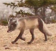
Image

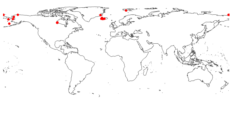
Arctic Fox

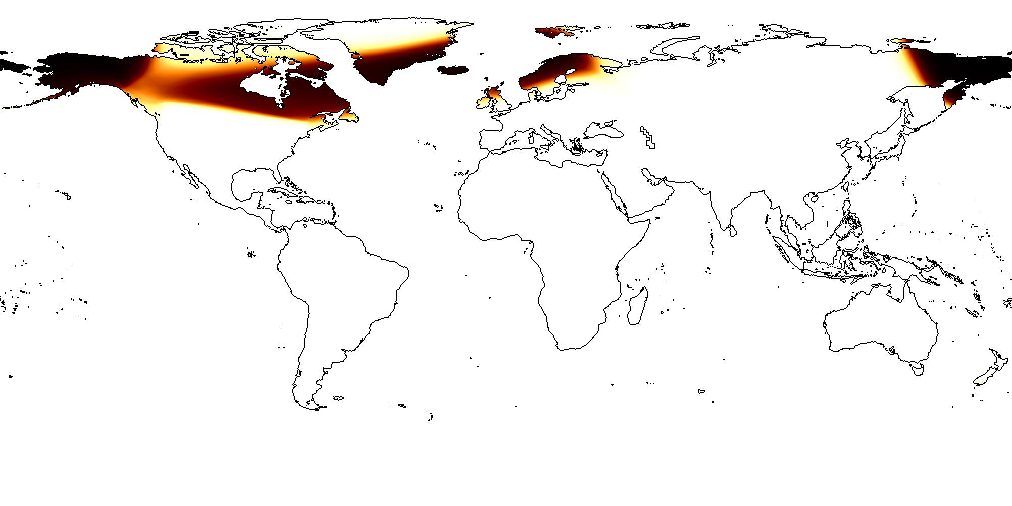
$wrap$

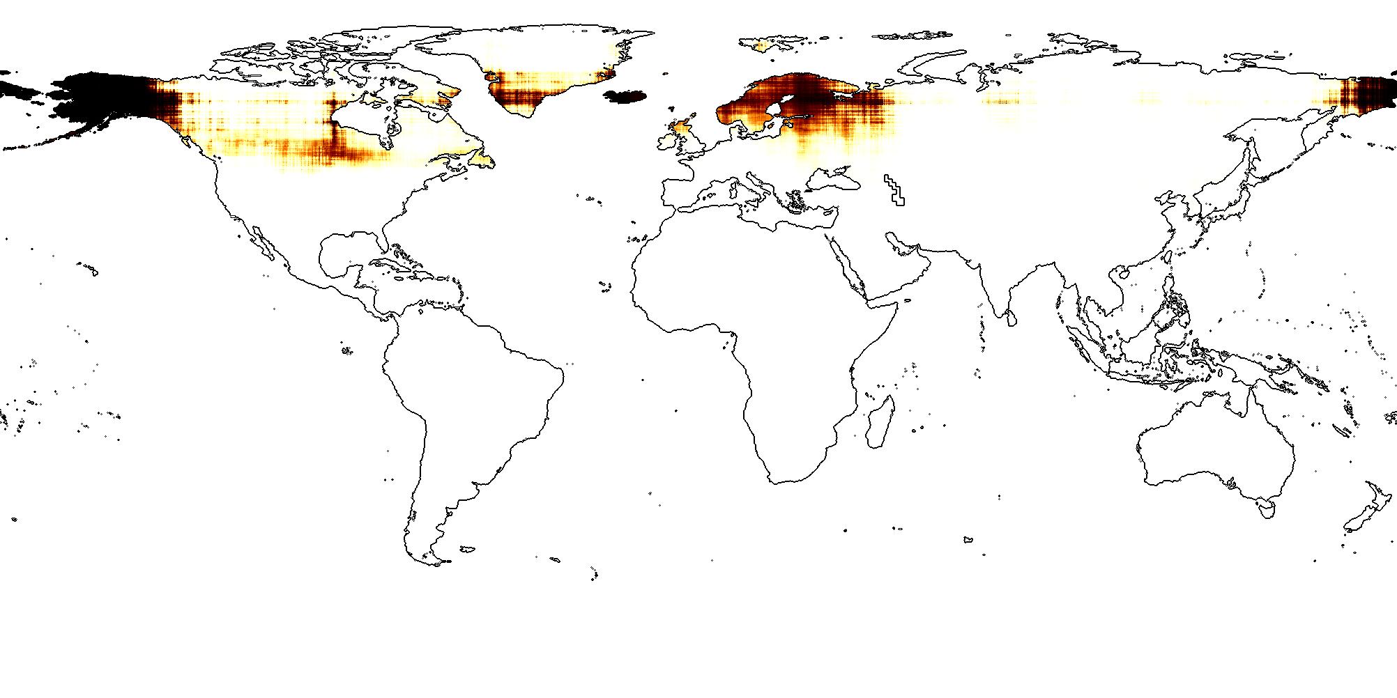
$grid$

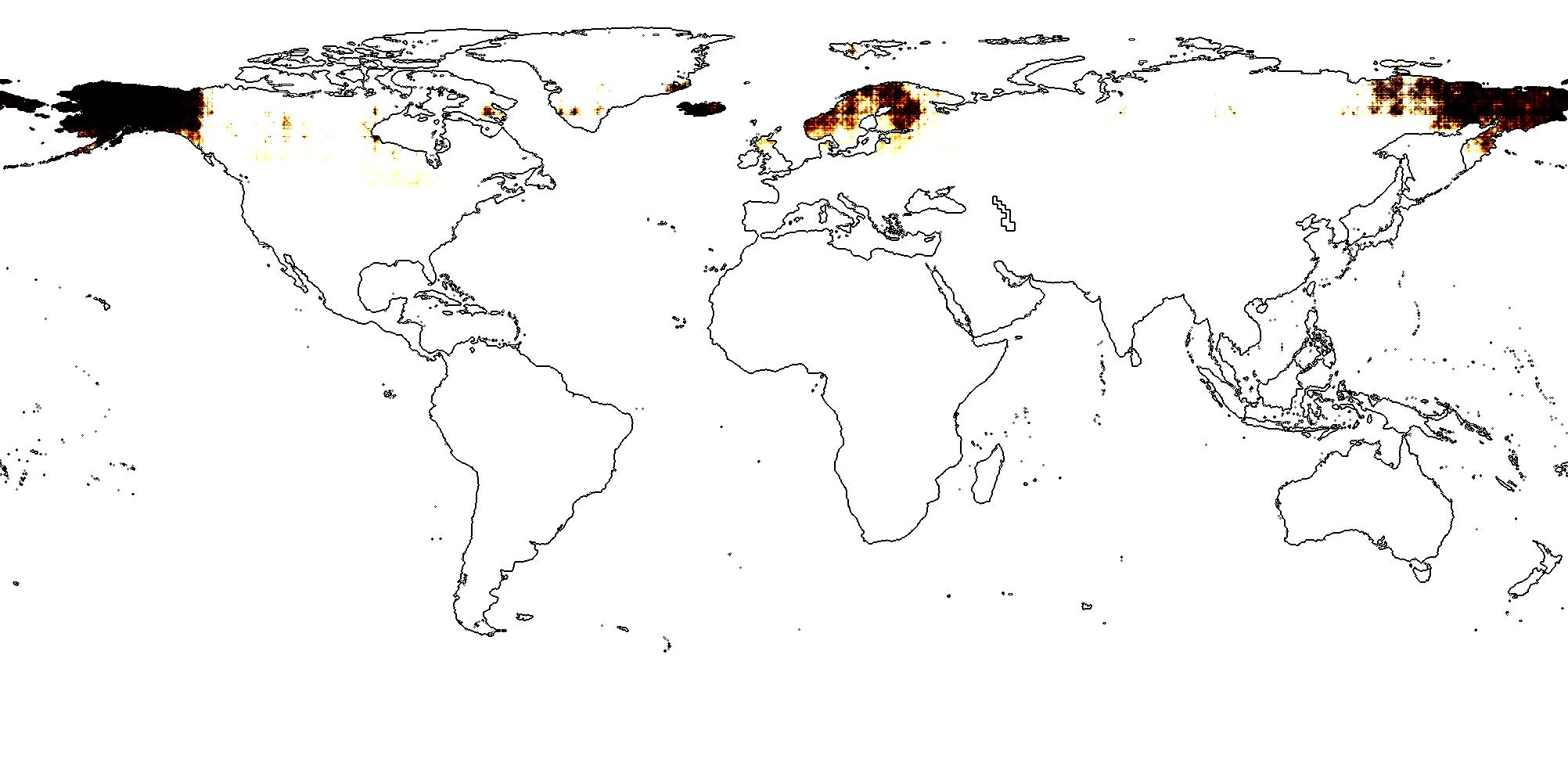
$sphereC+$

Image

Bat-Eared Fox

$wrap$

$grid$

$sphereC+$

Image

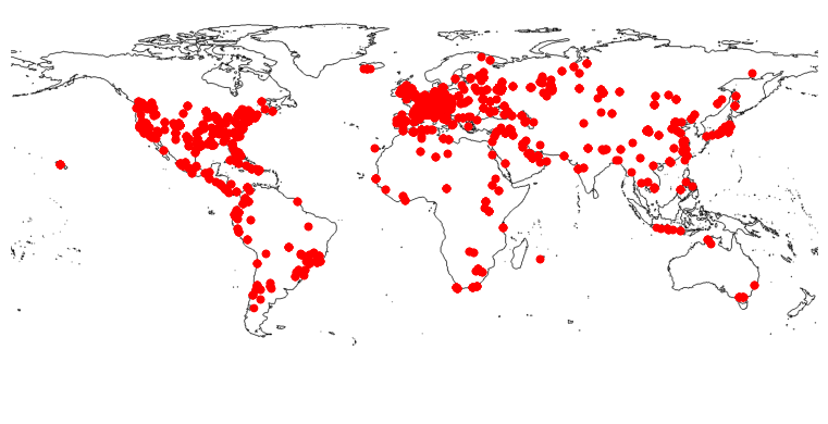
Factory or powerplant

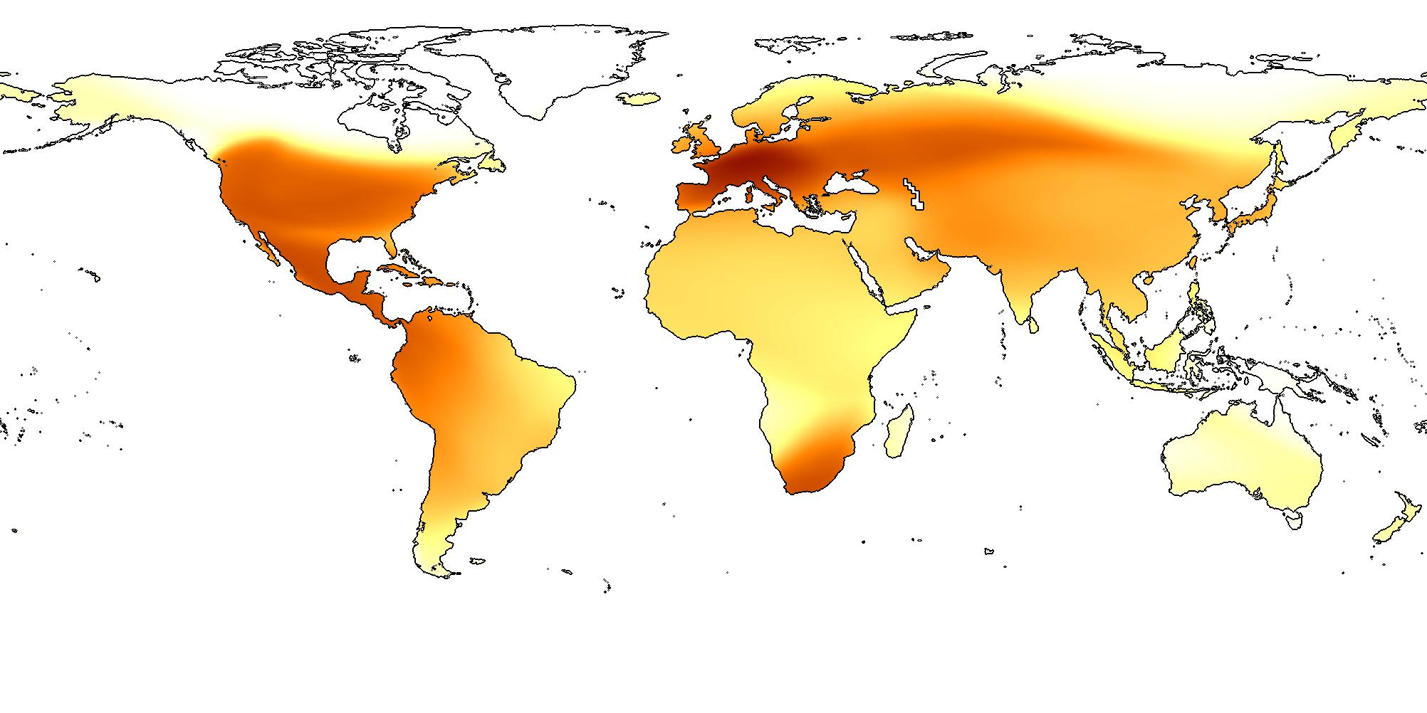
$wrap$

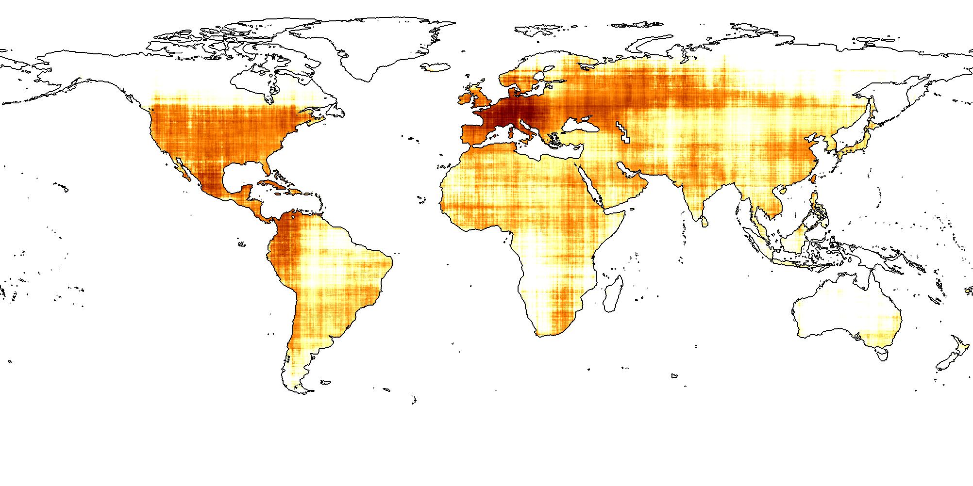
$grid$

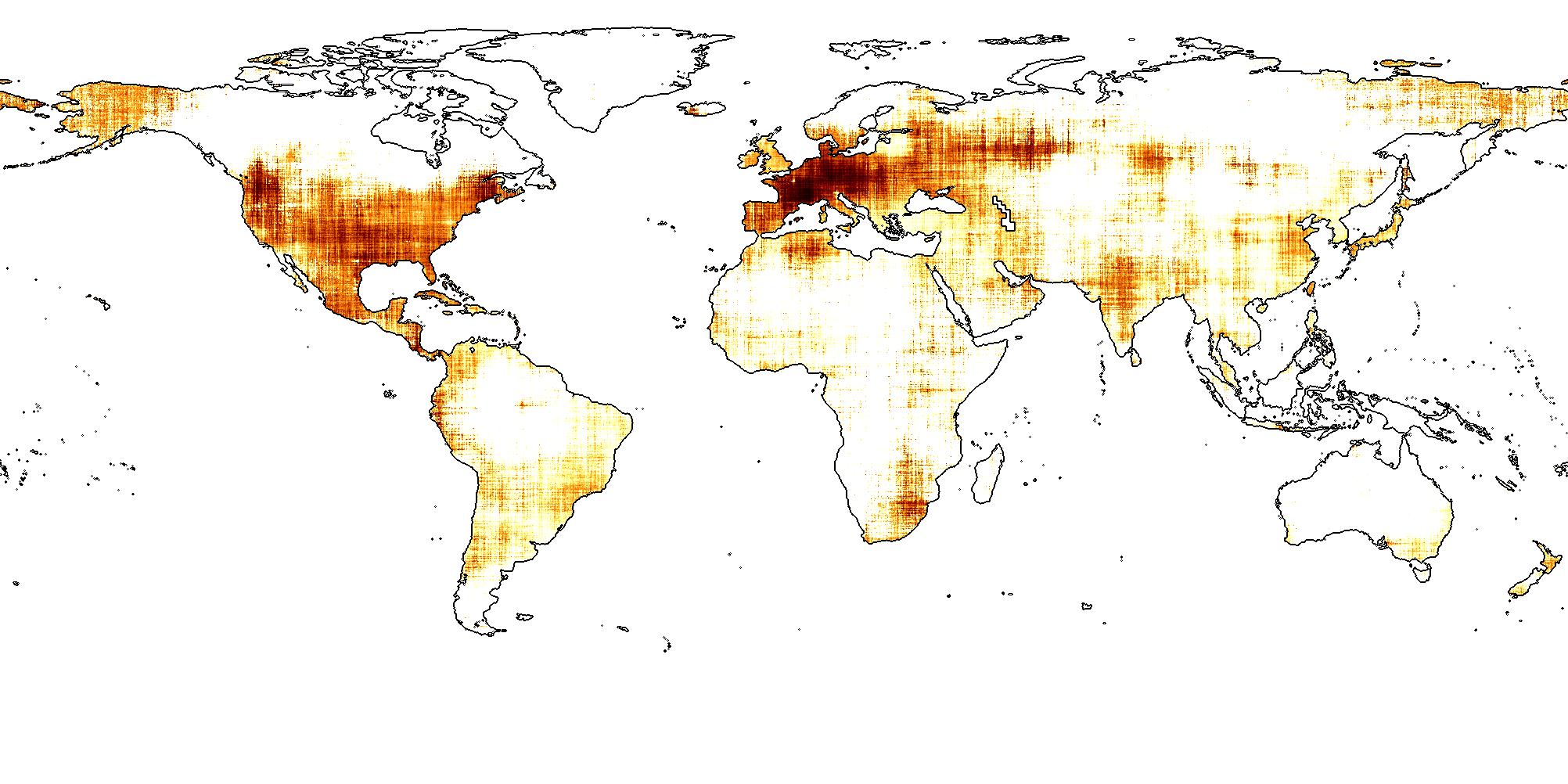
$dfs$

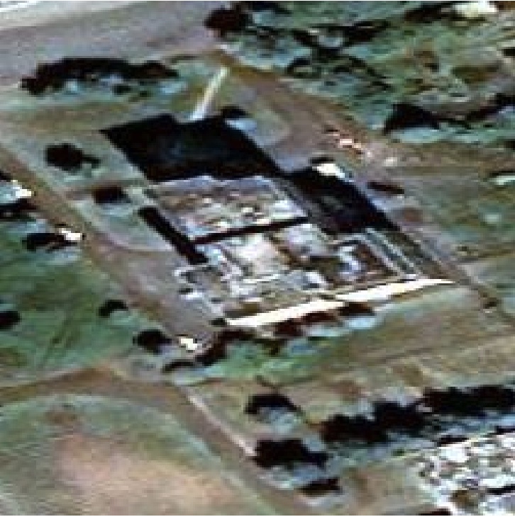
Image

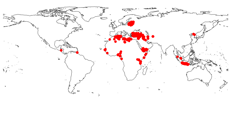
Multi-unit residential

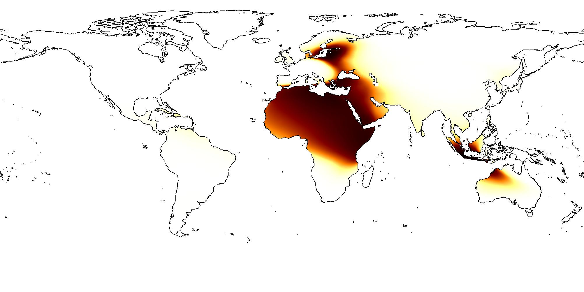
$wrap$

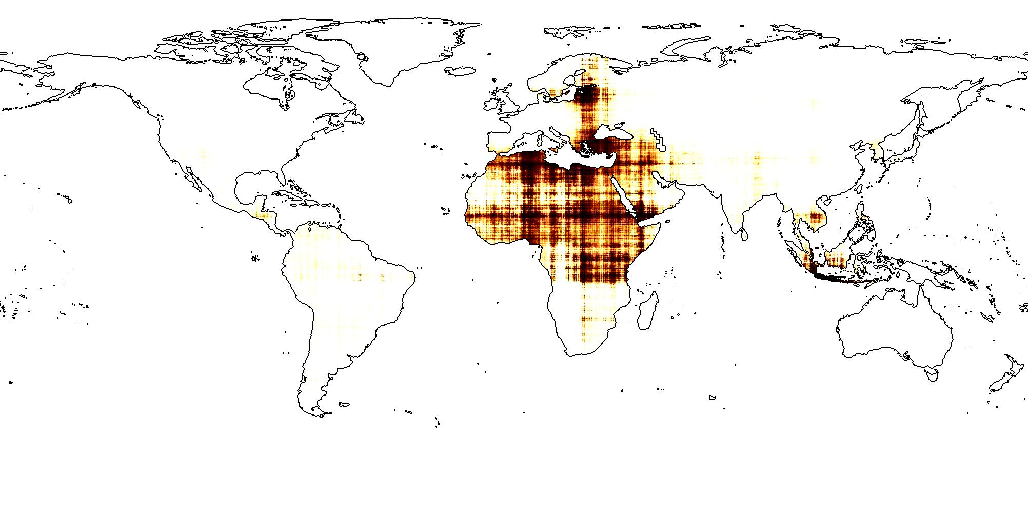
$grid$

$dfs$

Figure 2: Applying location encoders to differentiate two visually similar species ((a)-(j)) or two visually similar land use types ((k)-(t)). Arctic fox and bat-eared fox might look very similar visually as shown in (a) and (f). However, they have different spatial distributions. (b) and (g) show their distinct patterns in species image locations. (c)-(e): The predicted distributions of Arctic fox from different location encoders (without images as input). (h)-(j): The predicted distributions of bat-eared fox. Similarly, it might be hard to differentiate factories/powerplants from multi-unit residential buildings only based on their overhead satellite imgeries as shown in (k) and (p). However, as shown in (l) and (q), they have very different global spatial distributions. (m)-(o) and (r)-(t) show the predicted spatial distributions of factories/powerplants and multi-unit residential buildings from different location encoders. We can see that while $wrap$ (Mac Aodha et al., 2019) produces a over-generalized spatial distribution, $sphereC+$ and $dfs$ (our model) produces more compact and fine-grained distributions on the polar region and in data sparse areas such as Africa (See Figure 2-2). $grid$ (Mai et al., 2020b) is between the two. For more examples, please see Figure 13 and 14.

Subsequently, this practice of ignoring the round Earth has been adopted by many recent geospatial artificial intelligence (GeoAI) (Hu et al., 2019; Janowicz et al., 2020) research on problems such as climate extremes forecasting (Ham et al., 2019), species distribution modeling (Berg et al., 2014), location representation learning (Mai et al., 2020b), and trajectory prediction (Rao et al., 2020). Due to the lack of interpretability of these deep neural network models, this issue has not attracted much attentions by the whole geospatial community.

It is acceptable that the projection errors might be neglectable in small-scale (e.g., neighborhood-level or city-level) geospatial studies. However, they become non-negligible when we conduct research at a country scale or even global scale. Meanwhile, demand on representation and prediction learning at a global scale grows dramatically due to emerging global scale issues, such as the transition path of the latest pandemic (Chinazzi et al., 2020), long lasting issue for malaria (Caminade et al., 2014), under threaten global biodiversity (Di Marco et al., 2019; Ceballos et al., 2020), and numerous ecosystem and social system responses for climate change (Hansen and Cramer, 2015). This trend urgently calls for GeoAI models that can avoid map projection errors and directly perform calculation on a round planet (Chrisman, 2017). To achieve this goal, we need a representation learning model which can directly encode point coordinates on a spherical surface into the embedding space such that the resulting location embeddings preserve the spherical distances (e.g., great circle distance) between two points. With such a representation, existing neural network architectures can operate on spherical-distance-kept location embeddings to enable the ability of calculating on a round planet.

In fact, such location representation learning models are usually termed location encoders which were originally developed to handle 2D or 3D Cartesian coordinates (Chu et al., 2019; Mac Aodha et al., 2019; Mai et al., 2020b; Zhong et al., 2020; Mai et al., 2022b; Mildenhall et al., 2021; Schwarz et al., 2020; Niemeyer and Geiger, 2021; Barron et al., 2021; Marí et al., 2022; Xiangli et al., 2022). Location encoders represent a point in a 2D or 3D Euclidean space (Zhong et al., 2020; Mildenhall et al., 2021; Schwarz et al., 2020; Niemeyer and Geiger, 2021) into a high dimensional embedding such that the representations are more learning-friendly for downstream machine learning models. For example, Space2Vec  (Mai et al., 2020b, a) was developed for POI type classification, geo-aware image classification, and geographic question answering which can accurately model point distributions in a 2D Euclidean space. Recently, several popular location/position encoders widely used in the computer vision domain are also called neural implicit functions (Anokhin et al., 2021a; He et al., 2021; Chen et al., 2021; Niemeyer and Geiger, 2021) which follow the idea of Neural Radiance Fields (NeRF) (Mildenhall et al., 2020) to map a 2D or 3D point coordinates to visual signals via a Fourier input mapping (Tancik et al., 2020; Anokhin et al., 2021a; He et al., 2021), or so-called Fourier position encoding (Mildenhall et al., 2020; Schwarz et al., 2020; Niemeyer and Geiger, 2021), followed by a Multi-Layer Perception (MLP). Until now, those 2D/3D Euclidean location encoders have already shown promising performances on multiple tasks across different domains including geo-aware image classification (Chu et al., 2019; Mac Aodha et al., 2019; Mai et al., 2020b), POI classification (Mai et al., 2020b), trajectory prediction (Xu et al., 2018), geographic question answering (Mai et al., 2020a), 2D image superresolution(Anokhin et al., 2021a; Chen et al., 2021; He et al., 2021), 3D protein structure reconstruction (Zhong et al., 2020), 3D scenes representation for view synthesis (Mildenhall et al., 2020; Barron et al., 2021; Tancik et al., 2022; Marí et al., 2022; Xiangli et al., 2022) and novel image/view generation (Schwarz et al., 2020; Niemeyer and Geiger, 2021). However, similarly to above mentioned France case, when applying the state-of-the-art (SOTA) 2D Euclidean location encoders (Mac Aodha et al., 2019; Mai et al., 2020b) to large-scale real-world GPS coordinate datasets such as remote sensing images taken all over the world which require distance metric learning on the spherical surface, a map projection distortion problem (Williamson and Browning, 1973; Chrisman, 2017) emerges, especially in the polar areas. On the other hand, the NeRF-style 3D Euclidean location encoders (Mildenhall et al., 2020; Schwarz et al., 2020; Niemeyer and Geiger, 2021) are commonly used to model point distances in the 3D Euclidean space, but not capable of accurately modeling the distances on a complex manifold such as spherical surfaces. Directly applying NeRF-style models on these datasets means these models have to approximate the spherical distances with 3D Euclidean distances which leads to a distance metric approximation error. This highlights the necessity of such a spherical location encoder discussed above.

In this work, we propose a multi-scale spherical location encoder, Sphere2Vec, which can directly encode spherical coordinates while avoiding the map projection distortion and spherical-to-Euclidean distance approximation error. The multi-scale encoding method utilizes 2D Discrete Fourier Transform basis ($O(S^{2})$ terms) or a subset ($O(S)$ terms) of it while still being able to correctly measure the spherical distance. Following previous work we use location encoding to learn the geographic prior distribution of different image labels so that given an image and its associated location, we can combine the prediction of the location encoder and that from the state-of-the-art image classification models, e.g., inception V3 (Szegedy et al., 2016), to improve the image classification accuracy. Figure 1 illustrates the whole architecture. We demonstrate the effectiveness of Sphere2Vec on geo-aware image classification tasks including fine-grained species recognition (Chu et al., 2019; Mac Aodha et al., 2019; Mai et al., 2020b), Flickr image recognition (Tang et al., 2015; Mac Aodha et al., 2019), and remote sensing image classification (Christie et al., 2018; Ayush et al., 2020). Figure 2-2 and 2-2 show the predicted species distributions of Arctic fox and bat-eared fox from three different models. Figure 2-2 and 2-2 show the predicted land use distributions of factory or powerplant and multi-unit residential building from three different models. In summary, the contributions of our work are:

1. We propose a spherical location encoder, Sphere2Vec, which, as far as we know, is the first inductive embedding encoding scheme which aims at preserving spherical distance. We also developed a unified view of distant reserving encoding methods on spheres based on Double Fourier Sphere (DFS) (Merilees, 1973; Orszag, 1974).

2. We provide theoretical proof that Sphere2Vec encodings can preserve spherical surface distances between points. As a comparison, we also prove that the 2D location encoders (Gao et al., 2019; Mai et al., 2020b, 2023c) model latitude and longitude differences separately, and NeRF-style 3D location encoders (Mildenhall et al., 2020; Schwarz et al., 2020; Niemeyer and Geiger, 2021) model axis-wise differences between two points in 3D Euclidean space separately – none of them can correctly model spherical distances.

3. We first conduct experiments on 20 synthetic datasets generated based on the mixture of von Mises–Fisher distribution (MvMF). We show that Sphere2Vec is able to outperform all baselines including the state-of-the-art (SOTA) 2D location encoders and NeRF-style 3D location encoders on all 20 synthetic datasets with an up to 30.8% error rate reduction. Results show that 2D location encoders are more powerful than NeRF-style 3D location encoders on all synthetic datasets. And compared with those 2D location encoders, Sphere2Vec is more effective when the dataset has a large data bias toward the polar area.

4. We also conduct extensive experiments on seven real-world datasets for three geo-aware image classification tasks. Results show that due to its spherical distance preserving ability, Sphere2Vec outperforms both the SOTA 2D location encoder models and NeRF-style 3D location encoders.

5. Further analysis shows that compared with 2D location encoders, Sphere2Vec  is able to produce finer-grained and compact spatial distributions, and does significantly better in the polar regions and areas with sparse training samples.

The rest of this paper is structured as follows. In Section 2, we motivate our work by highlighting the importance of the idea of calculating on the round planet. Then, we provide a formal problem formulation of spherical location representation learning in Section 3. Next, we briefly summarize the related work in Section 4. The main contribution - Sphere2Vec - is detailed discussed in Section 5. Then, Section 6 lists all baseline models we consider in this work. The theoretical limitations of 2D location encoder $grid$ as well as NeRF style 3D location encoders are discussed in Section 7. Section 8 presents the experimental results on the synthetic datasets. Then, Section 9 presents our experimental results on 7 real-world datasets for geo-aware image classification. Finally, we conclude this paper in Section 10. Code and data of this work are available at https://gengchenmai.github.io/sphere2vec-website/.

Mercator

Miller

Sinusoidal

Equirectangular

Figure 3: An illustration for map projection distortion: (a)-(d): Tissot indicatrices for four projections. The equal area circles are putted in different locations to show how the map distortion affect its shape.

2 Calculating on a Round Planet

The blindness to the round Earth or the inappropriate usage of map projections can lead to tremendous and unexpected effects especially when we study a global scale problem since map projection distortion is unavoidable when projecting spherical coordinates into 2D space.

There are no map projection can preserve distances at all direction. The so-called equidistant projection can only preserve distance on one direction, e.g., the longitude direction for the equirectangular projection (See Figure 3), while the conformal map projections (See Figure 3) can preserve directions while resulting in a large distance distortion. For a comprehensive overview of map projections and their distortions, see Mulcahy and Clarke (2001).

When we estimate probability distributions at a global scale (e.g., species distributions or land use types over the world) with a neural network architecture, using 2D Euclidean-based GeoAI models with projected spatial data instead of directly modeling these distributions on a spherical surface will lead to unavoidable map projection distortions and suboptimal results. This highlights the importance of calculating on a round planet (Chrisman, 2017) and necessity of a spherical distance-kept location encoder.

3 Problem Formulation

Distributed representation of point-features on the spherical surface can be formulated as follows. Given a set of points $\mathcal{P}=\{\boldsymbol{\mathbf{x}}_{i}\}$ on the surface of a sphere $\mathbb{S}^{2}$, e.g., locations of remote sensing images taken all over the world, where $\boldsymbol{\mathbf{x}}_{i}=(\lambda_{i},\phi_{i})\in\mathbb{S}^{2}$ indicates a point with longitude $\lambda_{i}\in[-\pi,\pi)$ and latitude $\phi_{i}\in[-{\pi}/{2},{\pi}/{2}]$. Define a function $Enc_{\mathcal{P},\theta}(\boldsymbol{\mathbf{x}}):\mathbb{S}^{2}\to\mathbb{R}^{d}$, which is parameterized by $\theta$ and maps any coordinate $\boldsymbol{\mathbf{x}}$ in a spherical surface $\mathbb{S}^{2}$ to a vector representation of $d$ dimension. In the following, we use $Enc(\boldsymbol{\mathbf{x}})$ as an abbreviation for $Enc_{\mathcal{P},\theta}(\boldsymbol{\mathbf{x}})$.

Let $Enc(\boldsymbol{\mathbf{x}})=\mathbf{NN}(PE_{S}(\boldsymbol{\mathbf{x}}))$ where $\mathbf{NN}()$ is a learnable multi-layer perceptron with $h$ hidden layers and $k$ neurons per layer. We want to find a position encoding function $PE_{S}(\boldsymbol{\mathbf{x}})$ which does a one-to-one mapping from each point $\boldsymbol{\mathbf{x}}_{i}=(\lambda_{i},\phi_{i})\in\mathbb{S}^{2}$ to a multi-scale representation with $S$ be the total number of scales.

We expect to find a function $PE_{S}(\boldsymbol{\mathbf{x}})$ such that the resulting multi-scale representation of $\boldsymbol{\mathbf{x}}$ preserves the spherical surface distance while it is more learning-friendly for the downstream neuron network model $\mathbf{NN}()$. More concretely, we’d like to use position encoding functions which satisfy the following requirement:

$$\langle PE_{S}(\boldsymbol{\mathbf{x}}_{1}),PE_{S}(\boldsymbol{\mathbf{x}}_{2})\rangle=f(\Delta D),\forall\boldsymbol{\mathbf{x}}_{1},\boldsymbol{\mathbf{x}}_{2}\in\mathbb{S}^{2},$$ (1)

where $\langle\cdot,\cdot\rangle$ is the cosine similarity function between two embeddings. $\Delta D\in[0,\pi R]$ is the spherical surface distance between $\boldsymbol{\mathbf{x}}_{1},\boldsymbol{\mathbf{x}}_{2}$, $R$ is the radius of this sphere, and $f(x)$ is a strictly monotonically decreasing function for $x\in[0,\pi R]$.

4 Related Work

4.1 Neural Implicit Functions and NeRF

As an increasingly popular family of models in the computer vision domain, neural implicit functions (Anokhin et al., 2021a; He et al., 2021; Chen et al., 2021; Niemeyer and Geiger, 2021) refer to the neural network architectures that directly map a 2D or 3D coordinates into visual signals via a Fourier input mapping/position encoding (Tancik et al., 2020; Anokhin et al., 2021a; He et al., 2021; Mildenhall et al., 2020; Schwarz et al., 2020; Niemeyer and Geiger, 2021), followed by a Multi-Layer Perception (MLP).

A good example is Neural Radiance Fields (NeRF) (Mildenhall et al., 2020), which combines neural implicit functions and volume rendering for novel view synthesis for 3D complex scenes. The idea of NeRF  becomes very popular and many follow-up works have been done to revise the $NeRF$ model in order to achieve more accurate view synthesis. For example, NeRF in the Wild (NeRF-W) (Martin-Brualla et al., 2021) was proposed to learn separate transient phenomena from each static scene to make the model robust to radiometric variation and transient objects. Shadow NeRF (S-NeRF) (Derksen and Izzo, 2021) was proposed to exploit the direction of solar rays to obtain a more realistic view synthesis on multi-view satellite photogrammetry. Similarly, Satellite NeRF (Sat-NeRF) (Marí et al., 2022) combines NeRF with native satellite camera models to achieve robustness to transient phenomena that cannot be explained by the position of the sun to solve the same task. A more noticeable example is GIRAFFE (Niemeyer and Geiger, 2021) which is a NeRF-based deep generative model which achieves a more controllable image synthesis. All these NeRF variations mentioned above use the same NeRF Fourier position encoding. And they all use this position encoding in the same generative task – novel image synthesis. Moreover, although S-NeRF and Sat-NeRF work on geospatial data, i.e., satellite images, they focus on rather small geospatial scales, e.g., city scales, in which map projection distortion can be ignored. In contrast, we investigate the advantages and drawbacks of various location encoders in large-scale (e.g., global-scale) geospatial prediction tasks which are discriminative tasks. We use NeRF position encoding as one of our baselines.

Several works also discussed the possibility to revise NeRF position encoding. The original encoding method takes a single 3D point as input which ignores both the relative footprint of the corresponding image pixel and the length of the interval along the ray which leads to aliasing artifacts when rendering novel camera trajectories (Tancik et al., 2022). To fix this issue, Mip-NeRF (Barron et al., 2021) proposed a new Fourier position encoding called integrated positional encoding (IPE). Instead of encoding one single 3D point, IPE encodes 3D conical frustums approximated by multivariate Gaussian distributions which are sampled along the ray based on the projected pixel footprints. Block-NeRF (Tancik et al., 2022) adopted the IPE idea and showed how to scale NeRF to render city-scale scenes. Similarly, BungeeNeRF (Xiangli et al., 2022) also used the IPE model to develop a progressive NeRF that can do multi-scale rendering for satellite images in different spatial scales. In this work, we focus on encoding a single point on the spherical surface, not a 3D conical frustums. So IPE is not considered as one of the baselines.

Neural implicit functions are also popular for other computer vision tasks such as image superresolution (Anokhin et al., 2021a; Chen et al., 2021; He et al., 2021) and image compression (Dupont et al., ; Strümpler et al., 2022).

4.2 Location Encoder

Location encoders (Chu et al., 2019; Mac Aodha et al., 2019; Mai et al., 2020b; Zhong et al., 2020; Mai et al., 2023c) are neural network architectures which encode points in low-dimensional (2D or 3D) spaces (Zhong et al., 2020)) into high dimensional embeddings. There has been much research on developing inductive learning-based location encoders. Most of them directly apply Multi-Layer Perceptron (MLP) to 2D coordinates to get a high dimensional location embedding for downstream tasks such as pedestrian trajectory prediction (Xu et al., 2018) and geo-aware image classification (Chu et al., 2019). Recently, Mac Adoha et al. (Mac Aodha et al., 2019) apply sinusoid functions to encode the latitude and longitude of each image before feeding into MLPs. All of the above approaches deploy location encoding at a single-scale.

Inspired by the position encoder in Transformer (Vaswani et al., 2017) and Neuroscience research on grid cells (Banino et al., 2018; Cueva and Wei, 2018) of mammals, Mai et al. (2020b) proposed to apply multi-scale sinusoid functions to encode locations in 2D Euclidean space before feeding into MLPs. The multi-scale representations have advantage of capturing spatial feature distributions with different characteristics. Similarly, Zhong et al. (2020) utilized a multi-scale location encoder for the position of proteins’ atoms in 3D Euclidean space for protein structure reconstruction with great success. Location encoders can be incorporated into the state-of-art models for many tasks to make them spatially explicit (Yan et al., 2019a; Janowicz et al., 2020; Mai et al., 2022a, 2023c).

Compared with well-established kernel-based approaches (Schölkopf, 2001; Xu et al., 2018) such as Radius Based Function (RBF) which requires memorizing the training examples as the kernel centers for a robust prediction, inductive-learning-based location encoders (Chu et al., 2019; Mac Aodha et al., 2019; Mai et al., 2020b; Zhong et al., 2020) have many advantages: 1) They are more memory efficient since they do not need to memorize training samples; 2) Unlike RBF, the performance on unseen locations does not depend on the number and distribution of kernels. Moreover, Gao et al. (2019) have shown that grid-like periodic representation of locations can preserve absolute position information, relative distance, and direction information in 2D Euclidean space. Mai et al. (2020b) further show that it benefits the generalizability of down-stream models. For a comprehensive survey of different location encoders, please refer to Mai et al. (2022b).

Despite all these successes in location encoding research, none of them consider location representation learning on a spherical surface which is in fact critical for a global scale geospatial study. Our work aims at filling this gap.

4.3 Machine Learning Models on Spheres

Recently, there has been an increasing amount of work on designing machine learning models for prediction tasks on spherical surfaces. For the omnidirectional image classification task, both Cohen et al. (2018) and Coors et al. (2018) designed different spherical versions of the traditional convolutional neural network (CNN) models in which the CNN filters explicitly consider map projection distortion. In terms of image geolocalization (Izbicki et al., 2019a) and text geolocalization (Izbicki et al., 2019b), a loss function based on the mixture of von Mises-Fisher distributions (MvMF)– a spherical analog of the Gaussian mixture model (GMM)– is used to replace the traditional cross-entropy loss for geolocalization models (Izbicki et al., 2019a, b). All these works are closely related to geometric deep learning (Bronstein et al., 2017). They show the importance to consider the spherical geometry instead of projecting it back to a 2D plane, yet none of them considers representation learning of spherical coordinates in the embedding space.

4.4 Spatially Explicit Artificial Intelligence

There has been much work in improving the performance of current state-of-the-art artificial intelligence and machine learning models by using spatial features or spatial inductive bias – so-called spatially explicit artificial intelligence (Yan et al., 2017; Mai et al., 2019; Yan et al., 2019a, b; Janowicz et al., 2020; Li et al., 2021; Zhu et al., 2021; Janowicz et al., 2022; Liu and Biljecki, 2022; Zhu et al., 2022; Mai et al., 2022a, 2023b; Huang et al., 2023), or SpEx-AI. The spatial inductive bias in these models includes: spatial dependency (Kejriwal and Szekely, 2017; Yan et al., 2019a), spatial heterogeneity (Berg et al., 2014; Chu et al., 2019; Mac Aodha et al., 2019; Mai et al., 2020b; Zhu et al., 2021; Gupta et al., 2021; Xie et al., 2021), map projection (Cohen et al., 2018; Coors et al., 2018; Izbicki et al., 2019a, b), scale effect (Weyand et al., 2016; Mai et al., 2020b), and so on.

4.5 Pseudospectral Methods on Spheres

Multiple studies have been focused on the numerical solutions on spheres, for example, in weather prediction (Orszag, 1972, 1974; Merilees, 1973). The main idea is so-called pseudospectral methods which leverage truncated discrete Fourier transformation on spheres to achieve computation efficiency while avoiding the error caused by map projection distortion. The particular set of basis functions to be used depends on the particular problem. However, they do not aim at learning good representations in machine learning models. In this study, we try to make connections to these approaches and explore how their insights can be realized in a deep learning model.

5 Method

Our main contribution - the design of spherical distance-kept location encoder $Enc(\boldsymbol{\mathbf{x}})$, Sphere2Vec will be presented in Section 5.1. We developed a unified view of distance-reserving encoding on spheres based on Double Fourier Sphere (DFS) (Merilees, 1973; Orszag, 1974). The resulting location embedding $\mathbf{p}[\boldsymbol{\mathbf{x}}]=Enc(\boldsymbol{\mathbf{x}})$ is a general-purpose embedding which can be utilized in different decoder architectures for various tasks. In Section 5.2, we briefly show how to utilize the proposed $Enc(\boldsymbol{\mathbf{x}})$ in the geo-aware image classification task.

5.1 Sphere2Vec

The multi-scale location encoder defined in Section 3 is in the form of $Enc(\boldsymbol{\mathbf{x}})=\mathbf{NN}(PE_{S}(\boldsymbol{\mathbf{x}}))$. $PE_{S}(\boldsymbol{\mathbf{x}})$ is a concatenation of multi-scale spherical spatial features of $S$ levels. In the following, we call $Enc(\boldsymbol{\mathbf{x}})$ location encoder and its component $PE_{S}(\boldsymbol{\mathbf{x}})$ position encoder.

$dfs$

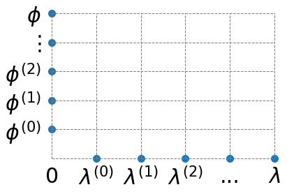
$grid$

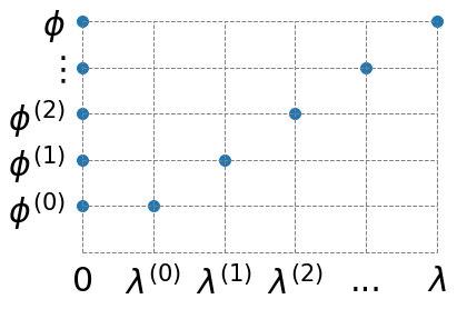
$sphereC$

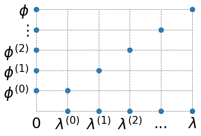
$sphereC+$

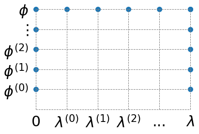
$sphereM$

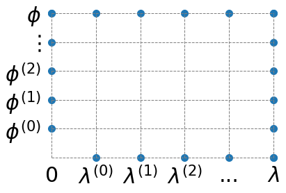
$sphereM+$

Figure 4: Patterns of different encoders, blue points at $(\lambda^{(m)},\phi^{(n)})$ mean interaction terms of trigonometric functions of $\lambda^{(m)}$ and $\phi^{(n)}$ are included in the encoder, $\lambda$ and $\phi$ axis correspond to single terms with no interactions.

$dfs$

Double Fourier Sphere (DFS) (Merilees, 1973; Orszag, 1974) is a simple yet successful pseudospectral method, which is computationally efficient and have been applied to analysis of large scale phenomenons such as weather (Sun et al., 2014) and blackholes (Bartnik and Norton, 2000). Our first intuition is to use the base functions of DFS, which preserve periodicity in both the longitude and latitude directions, to help decompose $\boldsymbol{\mathbf{x}}=(\lambda,\phi)$ into a high dimensional vector:

$$\begin{split}PE^{dfs}_{S}(\boldsymbol{\mathbf{x}})=&\bigcup_{n=0}^{S-1}[\sin\phi^{(n)},\cos\phi^{(n)}]\cup\bigcup_{m=0}^{S-1}[\sin\lambda^{(m)},\cos\lambda^{(m)}]\cup\\ &\bigcup_{n=0}^{S-1}\bigcup_{m=0}^{S-1}[\cos\phi^{(n)}\cos\lambda^{(m)},\cos\phi^{(n)}\sin\lambda^{(m)},\\ &\sin\phi^{(n)}\cos\lambda^{(m)},\sin\phi^{(n)}\sin\lambda^{(m)}],\end{split}$$ (2)

where $\lambda^{(m)}=\frac{\lambda}{r^{(m)}}$, $\phi^{(n)}=\frac{\phi}{r^{(n)}}$. $r^{(m)}$ and $r^{(n)}$ are scaling factors controlled by the current scale $m$ and $n$. Let $r_{min},r_{max}$ be the minimum and maximum scaling factor, and $g=\frac{r_{max}}{r_{min}}$. $r^{(s)}=r_{min}\cdot g^{s/(S-1)}$ where $s$ is either $m$ or $n$. $\cup$ means vector concatenation and $\bigcup_{s=0}^{S-1}$ indicates vector concatenation through different scales. It basically lets all the $S$ scales of $\phi$ terms interact with all the $S$ scales of $\lambda$ terms in the encoder. This would introduce a position encoder with a $O(S^{2})$ dimension output which increases the memory burden in training and hurts generalization. See Figure 4 for an illustration of the used $O(S^{2})$ terms. An encoder might achieve better results by only using a subset of these terms.

In comparison, the state-of-the-art $grid$ (Mai et al., 2020b) encoder defines its position encoder as:

$$PE^{grid}_{S}(\boldsymbol{\mathbf{x}})=\bigcup_{s=0}^{S-1}[\sin\phi^{(s)},\cos\phi^{(s)},\sin\lambda^{(s)},\cos\lambda^{(s)}].$$ (3)

Here, $\lambda^{(s)}$ and $\phi^{(s)}$ have similar definitions as $\lambda^{(m)}$ and $\phi^{(n)}$ in Equation 2. Figure 4 illustrates the used terms of $grid$. We can see that $grid$ employs a subset of terms from $dfs$. However, as we explained earlier, $grid$ performs poorly at a global scale due to its inability to preserve spherical distances.

In the following we explore different subsets of DFS terms while achieving two goals: 1) efficient representation with $O(S)$ dimensions 2) preserving distance measures on a spherical surface.

$sphereC$

Inspired by the fact that any point $(x,y,z)$ in 3D Cartesian coordinate can be expressed by $sin$ and $cos$ basis of spherical coordinates ($\lambda$, $\phi$ plus radius) , we define the basic form of Sphere2Vec, namely $sphereC$ encoder:

$$PE^{sphereC}_{S}(\boldsymbol{\mathbf{x}})=\bigcup_{s=0}^{S-1}[\sin\phi^{(s)},\cos\phi^{(s)}\cos\lambda^{(s)},\cos\phi^{(s)}\sin\lambda^{(s)}].$$ (4)

Figure 4 illustrates the used terms of $sphereC$. To illustrate that $sphereC$ is good at capturing spherical distance, we take a close look at its basic case $S=1$. When $S=1$ and $r_{max}=1$, there is only one scale $s=S-1=0$ and we define $r^{(s)}=r_{min}\cdot g^{s/(S-1)}=r_{max}=1$. The multi-scale encoder degenerates to

$$PE^{sphereC}_{1}(\boldsymbol{\mathbf{x}})=[\sin(\phi),\cos(\phi)\cos(\lambda),\cos(\phi)\sin(\lambda)].$$ (5)

These three terms are included in the multi-scale version ($S>1$) and serve as the main terms at the largest scale and also the lowest frequency (when $s=S-1$). The high frequency terms are added to help the downstream neuron network to learn the point-feature more efficiently (Tancik et al., 2020). Interestingly, $PE^{sphereC}_{1}$ captures the spherical distance in a very explicit way:

Theorem 1.

Let $\boldsymbol{\mathbf{x}}_{1}$, $\boldsymbol{\mathbf{x}}_{2}$ be two points on the same sphere $\mathbb{S}^{2}$ with radius $R$, then

$$\langle PE^{sphereC}_{1}(\boldsymbol{\mathbf{x}}_{1}),PE^{sphereC}_{1}(\boldsymbol{\mathbf{x}}_{2})\rangle=\cos(\frac{\Delta D}{R}),$$ (6)

where $\Delta D$ is the great circle distance between $\boldsymbol{\mathbf{x}}_{1}$ and $\boldsymbol{\mathbf{x}}_{2}$. Under this metric,

$$\|PE^{sphereC}_{1}(\boldsymbol{\mathbf{x}}_{1})-PE^{sphereC}_{1}(\boldsymbol{\mathbf{x}}_{2})\|=2\sin(\frac{\Delta D}{2R}).$$ (7)

Moreover, $\|PE^{sphereC}_{1}(\boldsymbol{\mathbf{x}}_{1})-PE^{sphereC}_{1}(\boldsymbol{\mathbf{x}}_{2})\|\approx\frac{\Delta D}{R}$,when $\Delta D$ is small w.r.t. $R$.

See the proof in Appendix A.1.

Since the central angle $\Delta\delta=\frac{\Delta D}{R}\in[0,\pi]$ and $\cos(x)$ is strictly monotonically decrease for $x\in[0,\pi],$ Theorem 1 shows that $PE^{sphereC}_{1}(\boldsymbol{\mathbf{x}})$ directly satisfies our expectation in Equation 1 where $f(x)=\cos(\frac{x}{R})$.

$sphereM$

Considering the fact that many geographical patterns are more sensitive to either latitude (e.g., temperature, sunshine duration) or longitude (e.g., timezones, geopolitical borderlines), we might want to focus on increasing the resolution of either $\phi$ or $\lambda$ while holding the other relatively at a large scale. Therefore, we introduce a multi-scale position encoder $sphereM$, where interaction terms between $\phi$ and $\lambda$ always have one of them fixed at the top scale:

$$\begin{split}PE^{sphereM}_{S}(\boldsymbol{\mathbf{x}})=&\bigcup_{s=0}^{S-1}[\sin\phi^{(s)},\cos\phi^{(s)}\cos\lambda,\cos\phi\cos\lambda^{(s)},\\ &\cos\phi^{(s)}\sin\lambda,\cos\phi\sin\lambda^{(s)}].\\ \end{split}$$ (8)

This new encoder ensures that the $\phi$ term interact with all the scales of $\lambda$ terms (i.e., $\lambda^{(s)}$ terms) and $\lambda$ term interact with all the scales of $\phi$ terms (i.e., $\phi^{(s)}$ terms). See Figure 4 for the used terms of $sphereM$. Both $PE^{sphereC}_{S}$ and $PE^{sphereM}_{S}$ are multi-scale versions of a spherical distance-kept encoder (See Equation 5) and keep that as the main term in their multi-scale representations.

$sphereC+$ and $sphereM+$

From the above analysis of the two proposed position encoders and the SOTA $grid$ encoders, we know that $grid$ pays more attention to the sum of $\cos$ difference of latitudes and longitudes, while our proposed encoders pay more attention to the spherical distances. In order to capture both information, we consider merging $grid$ with each proposed encoders to get more powerful models that encode geographical information from different angles.

$$PE^{sphereC+}_{S}(\boldsymbol{\mathbf{x}}) =PE^{sphereC}_{S}(\boldsymbol{\mathbf{x}})\cup PE^{grid}_{S}(\boldsymbol{\mathbf{x}}),$$ (9)

$$PE^{sphereM+}_{S}(\boldsymbol{\mathbf{x}}) =PE^{sphereM}_{S}(\boldsymbol{\mathbf{x}})\cup PE^{grid}_{S}(\boldsymbol{\mathbf{x}}).$$ (10)

We hypothesize that encoding these terms in the multi-scale representation would make the training of the encoder easier and the order of output dimension is still $O(S)$. See Figure 4 and 4 for the used terms of $sphereC+$ and $sphereM+$.

In location encoding, the uniqueness of the encoding results (i.e., no two different points on a sphere having the same position encoding) is very important. $PE_{S}(\boldsymbol{\mathbf{x}})$ in the five proposed methods are by design one-to-one mapping.

Theorem 2.

$\forall*\in\{dfs,sphereC,sphereC+,sphereM,$
$sphereM+\}$, $PE^{*}_{S}(\boldsymbol{\mathbf{x}})$ is an injective function.

See the proof in Appendix A.2.

5.2 Applying Sphere2Vec to Geo-Aware Image Classification

Follow the practice of Mac Aodha et al. (2019) and Mai et al. (2020b), we formulate the geo-aware image classification task (Chu et al., 2019; Mac Aodha et al., 2019) as follow: Given an image $\mathbf{I}$ taken from location/point $\boldsymbol{\mathbf{x}}$, we estimate which category $y$ it belongs to. If we assume that $\mathbf{I}$ and $\boldsymbol{\mathbf{x}}$ are independent given $y$ and an even-prior $P(y)$, then we have

$$P(y|\mathbf{I},\boldsymbol{\mathbf{x}})=\dfrac{P(\mathbf{I},\boldsymbol{\mathbf{x}}|y)P(y)}{P(\mathbf{I},\boldsymbol{\mathbf{x}})}=P(\mathbf{I}|y)P(\boldsymbol{\mathbf{x}}|y)\dfrac{P(y)}{P(\mathbf{I},\boldsymbol{\mathbf{x}})}$$ (11)

$$=\dfrac{P(y|\mathbf{I})P(\mathbf{I})}{P(y)}\dfrac{P(y|\boldsymbol{\mathbf{x}})P(\boldsymbol{\mathbf{x}})}{P(y)}\dfrac{P(y)}{P(\mathbf{I},\boldsymbol{\mathbf{x}})}$$ (12)

$$=P(y|\boldsymbol{\mathbf{x}})P(y|\mathbf{I})\dfrac{P(\mathbf{I})P(\boldsymbol{\mathbf{x}})}{P(y)P(\mathbf{I},\boldsymbol{\mathbf{x}})}\;\propto\;P(y|\boldsymbol{\mathbf{x}})P(y|\mathbf{I})$$ (13)

$P(y|\mathbf{I})$ can be obtained by fine-tuning the state-of-the-art image classification model for a specific task, such as a pretrained InceptionV3 network (Mac Aodha et al., 2019) for species recognition, or a pretrained MoCo-V2+TP (Ayush et al., 2020) for RS image classification. To be more specific, we use a pretrained image encoder $\mathbf{F}()$ to extract the embedding for each input image, i.e., $\mathbf{F}(\mathbf{I})$. Then in order to compute $P(y|\mathbf{I})$, we can either 1) fine-tune an image classifier $\mathbf{Q}$ based on these frozen image embeddings, or 2) fine-tune the whole image encoder architecture $\mathbf{Q}(\mathbf{F}(\mathbf{I}))$. Here, $\mathbf{Q}$ is a multilayer perceptron (MLP) followed by a softmax activation function. Both Mac Aodha et al. (2019) and Mai et al. (2020b) adopted the second approach which fine-tunes the whole image classification architecture. We also adopt the second approach to have a fair comparison with all these previous methods. Please refer to Section 9.4.3 for an ablation study on this. The idea is illustrated in the orange box in Figure 1.

In this work, we focus on the second component – estimating the geographic prior distribution of image label $y$ over the spherical surface $P(y|\boldsymbol{\mathbf{x}})$ (the blue box in Figure 1). This probability distribution can be estimated by using a location encoder $Enc()$. We can use either our proposed Sphere2Vec or some existing 2D (Mai et al., 2020b; Mac Aodha et al., 2019; Chu et al., 2019) or 3D (Marí et al., 2022; Martin-Brualla et al., 2021) Euclidean location encoders. More concretely, we have $P(y|\boldsymbol{\mathbf{x}})\;\propto\;\sigma(Enc(\boldsymbol{\mathbf{x}})\mathbf{T}_{:,y})$ where $\sigma()$ is a sigmoid activation function. $\mathbf{T}\in\mathbb{R}^{d\times c}$ is a class embedding matrix (the location classifier in Figure 1) where the $y_{th}$ column $\mathbf{T}_{:,y}\in\mathbb{R}^{d}$ indicates the class embedding for class $y$. $d$ indicates the dimension of location embedding $\mathbf{p}[\boldsymbol{\mathbf{x}}]=Enc(\boldsymbol{\mathbf{x}})$ and $c$ is the total number of image classes.

The major objective is to learn $P(y|\boldsymbol{\mathbf{x}})\;\propto\;\sigma(Enc(\boldsymbol{\mathbf{x}})\mathbf{T}_{:,y})$ such that all observed species occurrences (all image locations $\boldsymbol{\mathbf{x}}$ as well as their associated species class $y$) have maximum probabilities. Mac Aodha et al. (2019) used a loss function which is based on maximum likelihood estimation (MLE). Given a set of training samples - data points and their associated class labels $\mathbb{X}=\{(\boldsymbol{\mathbf{x}},y)\}$, the loss function $\mathcal{L}^{image}(\mathbb{X})$ is defined as:

$$\begin{split}\mathcal{L}^{image}(\mathbb{X})=&\sum_{(\boldsymbol{\mathbf{x}},y)\in\mathbb{X}}\sum_{\boldsymbol{\mathbf{x}}^{-}\in\mathcal{N}(\boldsymbol{\mathbf{x}})}\Big{(}\beta\log(\sigma(Enc(\boldsymbol{\mathbf{x}})\mathbf{T}_{:,y}))\\ &+\sum_{i=1,i\neq y}^{c}\log(1-\sigma(Enc(\boldsymbol{\mathbf{x}})\mathbf{T}_{:,i}))\\ &+\sum_{i=1}^{c}\log(1-\sigma(Enc(\boldsymbol{\mathbf{x}}^{-})\mathbf{T}_{:,i}))\Big{)}\end{split}$$ (14)

Here, $\beta$ is a hyperparameter to increase the weight of positive samples. $\mathcal{N}(\boldsymbol{\mathbf{x}})$ represents the negative sample set of point $\boldsymbol{\mathbf{x}}$ in which $\boldsymbol{\mathbf{x}}^{-}\in\mathcal{N}(\boldsymbol{\mathbf{x}})$ is a negative sample uniformly generated from the spherical surface given each data point $\boldsymbol{\mathbf{x}}$. Equation 14 can be seen as a modified version of the cross-entropy loss used in binary classification. The first term is the positive sample term weighted by $\beta$. The second term is the normal negative term used in cross-entropy loss. The third term is added to consider uniformly sampled locations as negative samples.

Figure 1 illustrates the whole workflow. During training time, the image classification module (the orange box) and location classification module (the blue box) are supervised trained separately. During the inference time, the probabilities $P(y|\mathbf{I})$ and $P(y|\boldsymbol{\mathbf{x}})$ computed from these two modules are multiplied to yield the final prediction.

6 Baselines

In order to understand the advantage of spherical-distance-kept location encoders, we compare different versions of Sphere2Vec with multiple baselines:

• $tile$ divides the study area $A$ (e.g., the earth’s surface) into grids with equal intervals along the latitude and longitude direction. Each grid has an embedding to be used as the encoding for every location $\boldsymbol{\mathbf{x}}$ fall into this grid. This is a common practice adopted by many previous works when dealing with coordinate data (Berg et al., 2014; Adams et al., 2015; Tang et al., 2015).

• $wrap$ is a location encoder model introduced by Mac Aodha et al. (2019). Given a location $\boldsymbol{\mathbf{x}}=(\lambda,\phi)$, it uses a coordinate wrap mechanism to convert each dimension of $\boldsymbol{\mathbf{x}}$ into 2 numbers :

  $$PE^{wrap}_{1}(\boldsymbol{\mathbf{x}})=[\sin(\lambda),\cos(\lambda),\sin(2\phi),\cos(2\phi)].$$ (15)

  Then the results are passed through a multi-layered fully connected neural network $\mathbf{NN}^{wrap}()$ which consists of an initial fully connected layer, followed by a series of $h$ residual blocks, each consisting of two fully connected layers ($k$ hidden neurons) with a dropout layer in between. We adopt the official code of Mac Aodha et al. (2019) for this implementation. We can see that $wrap$ still follows our general definition of location encoders $Enc(\boldsymbol{\mathbf{x}})=\mathbf{NN}(PE_{S}(\boldsymbol{\mathbf{x}}))$ where $S=1$.

• $wrap+ffn$ is similar to $wrap$ except that it replaces $\mathbf{NN}^{wrap}()$ with $\mathbf{NN}^{ffn}()$, a simple learnable multi-layer perceptron with $h$ hidden layers and $k$ neurons per layer as that Sphere2Vec has. $wrap+ffn$ is used to exclude the effect of different $\mathbf{NN}()$ on the performance of location encoders. In the following, all location encoder baselines use $\mathbf{NN}^{ffn}()$ as the learnable neural network component so that we can directly compare the effect of different position encoding $PE^{*}_{S}$ on the model performance.

• $xyz$ first converts $\boldsymbol{\mathbf{x}}_{i}=(\lambda_{i},\phi_{i})\in\mathbb{S}^{2}$ into 3D Cartesian coordinates $(x,y,z)$ centered at the sphere center by following Equation 16 before feeding into a multilayer perceptron $\mathbf{NN}()$. Here, we let $(x,y,z)$ to locate on a unit sphere with radius $R=1$. As we can see, $xyz$ is just a special case of $sphereC$ when $S=1$, i.e., $PE^{sphereC}_{1}$.

  $$\begin{split}PE^{xyz}_{S}(\boldsymbol{\mathbf{x}})&=[z,x,y]=PE^{sphereC}_{1}\\ &=[\sin\phi,\cos\phi\cos\lambda,\cos\phi\sin\lambda]\end{split}$$ (16)

• ${rbf}$ randomly samples $M$ points from the training dataset as RBF anchor points {$\boldsymbol{\mathbf{x}}^{anchor}_{m},m=1...M$}, and use gaussian kernels $\exp{\big{(}-\dfrac{\parallel\boldsymbol{\mathbf{x}}_{i}-\boldsymbol{\mathbf{x}}^{anchor}_{m}\parallel^{2}}{2\sigma^{2}}\big{)}}$ on each anchor points, where $\sigma$ is the kernel size. Each input point $\boldsymbol{\mathbf{x}}_{i}$ is encoded as a $M$-dimension RBF feature vector, i.e., $PE^{rbf}_{M}$, which is fed into $\mathbf{NN}^{ffn}()$ to obtain the location embedding. This is a strong baseline for representing floating number features in machine learning models used by Mai et al. (2020b).

• $rff$, i.e., Random Fourier Features (Rahimi and Recht, 2008; Nguyen et al., 2017), first encodes location $\boldsymbol{\mathbf{x}}$ into a $D$ dimension vector - $PE^{rff}_{D}(\boldsymbol{\mathbf{x}})=\varphi(\boldsymbol{\mathbf{x}})=\frac{\sqrt{2}}{\sqrt{D}}\bigcup_{i=1}^{D}[\cos{(\omega_{i}^{T}\boldsymbol{\mathbf{x}}+b_{i})}]$ where $\omega_{i}\overset{i.i.d}{\sim}\mathcal{N}(\mathbf{0},\delta^{2}I)$ is a direction vector whose each dimension is independently sampled from a normal distribution. $b_{i}$ is uniformly sampled from $[0,2\pi]$. $I$ is an identity matrix. Each component of $\varphi(\boldsymbol{\mathbf{x}})$ first projects $\boldsymbol{\mathbf{x}}$ into a random direction $\omega_{i}$ and makes a shift by $b_{i}$. Then it wraps this line onto the unit cirle in $\mathbb{R}^{2}$ with the cosine function. Rahimi and Recht (2008) show that $\varphi(\boldsymbol{\mathbf{x}})^{T}\varphi(\boldsymbol{\mathbf{x}}^{\prime})$ is an unbiased estimator of the Gaussian kernal $K(\boldsymbol{\mathbf{x}},\boldsymbol{\mathbf{x}}^{\prime})$. $\varphi(\boldsymbol{\mathbf{x}})$ is consist of $D$ different estimates to produce an approximation with a further lower variance. To make $rff$ comparable to other baselines, we feed $\varphi(\boldsymbol{\mathbf{x}})$ into $\mathbf{NN}^{ffn}()$ to produce the final location embedding.

• $grid$ is a multi-scale location encoder on 2D Euclidean space proposed by Mai et al. (2020b). Here, we simply treat $\boldsymbol{\mathbf{x}}=(\lambda,\phi)$ as 2D coordinate. It first use $PE^{grid}_{S}(\boldsymbol{\mathbf{x}})$ shown in Equation 3 to encode location $\boldsymbol{\mathbf{x}}$ into a multi-scale representation and then feed it into $\mathbf{NN}^{ffn}()$ to produce the final location embedding.

• $theory$ is another multi-scale location encoder on 2D Euclidean space proposed by Mai et al. (2020b). It use a position encoder $PE^{theory}_{S}(\boldsymbol{\mathbf{x}})$ shown in Equation 17. Here, $\boldsymbol{\mathbf{x}}^{(s)}=[\lambda^{(s)},\phi^{(s)}]=[\frac{\lambda}{r^{(s)}},\frac{\phi}{r^{(s)}}]$ and $\mathbf{a}_{1}=[1,0]^{T},\mathbf{a}_{2}=[-1/2,\sqrt{3}/2]^{T},\mathbf{a}_{3}=[-1/2,-\sqrt{3}/2]^{T}\in\mathbb{R}^{2}$ are three unit vectors which orient $2\pi/3$ apart from each other. The encoding results are feed into $\mathbf{NN}^{ffn}()$ to produce the final location embedding.

  $$PE^{theory}_{S}(\boldsymbol{\mathbf{x}})=\bigcup_{s=0}^{S-1}\bigcup_{j=1}^{3}[\sin(\langle\boldsymbol{\mathbf{x}}^{(s)},\mathbf{a}_{j}\rangle),\cos(\langle\boldsymbol{\mathbf{x}}^{(s)},\mathbf{a}_{j}\rangle)].$$ (17)

• $NeRF$ indicates a multiscale location encoder adapted from the positional encoder $PE^{NeRF}_{S}(\boldsymbol{\mathbf{x}})$ used by Neural Radiance Fields (NeRF) (Mildenhall et al., 2020) and many NeRF variations such as NeRF-W (Martin-Brualla et al., 2021), S-NeRF (Derksen and Izzo, 2021), Sat-NeRF (Marí et al., 2022), GIRAFFE (Niemeyer and Geiger, 2021), etc., which was proposed for novel view synthesis for 3D scenes. Here, $NeRF$ can be treated as a multiscale version of $xyz$. It first converts $\boldsymbol{\mathbf{x}}=(\lambda,\phi)\in\mathbb{S}^{2}$ into 3D Cartesian coordinates $(x,y,z)$ centered at the unit sphere center. Here, $(x,y,z)$ are normalized to lie in $[-1,1]$, i.e., $R=1$. Different from $xyz$, it uses NeRF-style positional encoder $PE^{NeRF}_{S}(\boldsymbol{\mathbf{x}})$ in Equation 18 to process $(x,y,z)$ into a multiscale representation. To make it comparable with other location encoders, we further feed $PE^{NeRF}_{S}(\boldsymbol{\mathbf{x}})$ into $\mathbf{NN}^{ffn}()$ to get the final location embedding.

  $$\begin{split}&PE^{NeRF}_{S}(\boldsymbol{\mathbf{x}})=\bigcup_{s=0}^{S-1}\bigcup_{p\in\{z,x,y\}}[\sin(2^{s}\pi p),\cos(2^{s}\pi p)],\\ &where\;[z,x,y]=[\sin\phi,\cos\phi\cos\lambda,\cos\phi\sin\lambda].\end{split}$$ (18)

All types of Sphere2Vec as well as all baseline models we compared except $tile$ share the same model set up - $Enc(\boldsymbol{\mathbf{x}})=\mathbf{NN}(PE_{S}(\boldsymbol{\mathbf{x}}))$. The main difference is the position encoder $PE_{S}(\boldsymbol{\mathbf{x}})$ used in different models. $PE_{S}(\boldsymbol{\mathbf{x}})$ used by $grid$, $theory$, $NeRF$, and different types of Sphere2Vec encode the input coordinates in a multi-scale fashion by using different sinusoidal functions with different frequencies. Many previous work call this practice “Fourier input mapping” (Rahaman et al., 2019; Tancik et al., 2020; Basri et al., 2020; Anokhin et al., 2021b). The difference is that $grid$ and $theory$ use the Fourier features from 2D Euclidean space, $NeRF$ uses the predefined Fourier scales to directly encode the points in 3D Euclidean space, while our Sphere2Vec uses all or the subset of Double Fourier Sphere Features to take into account the spherical geometry and the distance distortion it brings.

All models are implemented in PyTorch. We use the original implementation of $wrap$ from Mac Aodha et al. (2019) and the implementation of $grid$ and $theory$ from Mai et al. (2020b). Since the original implementation of NeRF (Mildenhall et al., 2020) is in TensorFlow, we reimplement $NeRF$ in PyTorch Framework by following their codes. We train and evaluate each model on a Ubuntu machine with 2 GeForce GTX Nvidia GPU cores, each of which has 10GB memory.

7 Theoretical Limitations of $grid$ and $NeRF$

7.1 Theoretical Limitations of $grid$

We first provide mathematic proofs to demonstrate why $grid$ is not suitable to model spherical distances.

Theorem 3.

Let $\boldsymbol{\mathbf{x}}_{1}$, $\boldsymbol{\mathbf{x}}_{2}$ be two points on the same sphere $\mathbb{S}^{2}$ with radius $R$, then we have

$$\begin{split}&\langle PE^{grid}_{S}(\boldsymbol{\mathbf{x}}_{1}),PE^{grid}_{S}(\boldsymbol{\mathbf{x}}_{2})\rangle\\ &=\sum_{s=0}^{S-1}\Big{(}\cos(\phi^{(s)}_{1}-\phi^{(s)}_{2})+\cos(\lambda^{(s)}_{1}-\lambda^{(s)}_{2})\Big{)}\\ &=\sum_{s=0}^{S-1}\Big{(}\cos(\frac{\phi_{1}-\phi_{2}}{r^{(s)}})+\cos(\frac{\lambda_{1}-\lambda_{2}}{r^{(s)}})\Big{)},\end{split}$$ (19)

When $S=1$, we have

$$\begin{split}\langle PE^{grid}_{1}(\boldsymbol{\mathbf{x}}_{1}),PE^{grid}_{1}(\boldsymbol{\mathbf{x}}_{2})\rangle=\cos(\phi_{1}-\phi_{2})+\cos(\lambda_{1}-\lambda_{2}),\end{split}$$ (20)

Theorem 3 is very easy to prove based on the angle difference formula, so we skip its proof. This result indicates that $grid$ models the latitude and longitude differences of $\boldsymbol{\mathbf{x}}_{1}$ and $\boldsymbol{\mathbf{x}}_{2}$ independently rather than spherical distance. This introduces problems when encoding locations in the polar area. Let’s consider data pairs $\boldsymbol{\mathbf{x}}_{1}=(\lambda_{1},\phi)$ and $\boldsymbol{\mathbf{x}}_{2}=(\lambda_{2},\phi)$, the distance between them in output space of $PE^{grid}_{S}$ is:

$$\begin{split}&\|PE^{grid}_{S}(\boldsymbol{\mathbf{x}}_{1})-PE^{grid}_{S}(\boldsymbol{\mathbf{x}}_{2})\|^{2}\\ &=\|PE^{grid}_{S}(\boldsymbol{\mathbf{x}}_{1})\|^{2}+\|PE^{grid}_{S}(\boldsymbol{\mathbf{x}}_{2})\|^{2}\\ &-2\langle PE^{grid}_{S}(\boldsymbol{\mathbf{x}}_{1}),PE^{grid}_{S}(\boldsymbol{\mathbf{x}}_{2})\rangle\\ &=2-2\sum_{s=0}^{S-1}\cos(\frac{\lambda_{1}-\lambda_{2}}{r^{(s)}})\end{split}$$ (21)

This distance stays as a constant for any values of $\phi$. However, when $\phi$ varies from $-\frac{\pi}{2}$ to $\frac{\pi}{2}$, the actual spherical distance changes in a wide range, e.g., the actual distance between the data pair at $\phi=-\frac{\pi}{2}$ (South Pole) is 0 while the distance between the data pair at $\phi=0$ (Equator), gets the maximum value. This problem in measuring distances also has a negative impact on $grid$’s ability to model distributions in areas with sparse sample points because it is hard to learn the true spherical distances.

In fact, in our experiments ($S>1$), we observe that $grid$ reaches peak performance at much smaller $r_{min}$ than that of Sphere2Vec encodings. Moreover, $sphereC$ outperforms $grid$ near polar regions where $grid$ produces large distances though the spherical distances are small (A, B in Figure 1).

7.2 Theoretical Limitations of $NeRF$

Since $NeRF$ is widely used for 3D representation learning (Mildenhall et al., 2020; Niemeyer and Geiger, 2021), a natural question is why not just use $NeRF$ for the geographic prediction tasks on the spherical surface, which can be embedded in the 3D space. In this section, we discuss the theoretical limitations of $NeRF$ 3D multiscale encoding in the scenario of spherical encoding.

Theorem 4.

Let $\boldsymbol{\mathbf{x}}_{1},\boldsymbol{\mathbf{x}}_{2}\in\mathbb{S}^{2}$ be two points on the spherical surface. Given their 3D Euclidean representations, i.e., $\boldsymbol{\mathbf{x}}_{1}=(z_{1},x_{1},y_{1})$, $\boldsymbol{\mathbf{x}}_{2}=(z_{2},x_{2},y_{2})$, we define $\Delta\boldsymbol{\mathbf{x}}=\boldsymbol{\mathbf{x}}_{1}-\boldsymbol{\mathbf{x}}_{2}=[z_{1}-z_{2},x_{1}-x_{2},y_{1}-y_{2}]=[\Delta\boldsymbol{\mathbf{x}}_{z},\Delta\boldsymbol{\mathbf{x}}_{x},\Delta\boldsymbol{\mathbf{x}}_{y}]$ as the difference between them in the 3D Euclidean space. Under $NeRF$ encoding (Equation 18), the distance between them satisfies

$$\begin{split}&\|PE^{NeRF}_{S}(\boldsymbol{\mathbf{x}}_{1})-PE^{NeRF}_{S}(\boldsymbol{\mathbf{x}}_{2})\|^{2}\\ &=\sum_{s=0}^{S-1}\Big{(}4\sin^{2}(2^{s-1}\pi\Delta\boldsymbol{\mathbf{x}}_{z})+4\sin^{2}(2^{s-1}\pi\Delta\boldsymbol{\mathbf{x}}_{x})\\ &+4\sin^{2}(2^{s-1}\pi\Delta\boldsymbol{\mathbf{x}}_{y})\Big{)}\\ &=\sum_{s=0}^{S-1}4\|\boldsymbol{\mathbf{Y}}_{s}\|^{2},\\ \end{split}$$ (22)

where $\boldsymbol{\mathbf{Y}}_{s}=[\sin(2^{s-1}\pi\Delta\boldsymbol{\mathbf{x}}_{z}),\sin(2^{s-1}\pi\Delta\boldsymbol{\mathbf{x}}_{x}),\sin(2^{s-1}\pi\Delta\boldsymbol{\mathbf{x}}_{y})]$.

See the proof in Appendix A.3.

Theorem 5.

$NeRF$ is not an injective function.

Theorem 5 is very easy to prove based on Theorem 4. Since $NeRF$ requires $R=1$, when $\boldsymbol{\mathbf{x}}_{1}=(1,0,0)$ and $\boldsymbol{\mathbf{x}}_{2}=(-1,0,0)$, i.e., they are the north and south pole, we have $\Delta\boldsymbol{\mathbf{x}}=[2,0,0]$. The distance between their multiscale $NeRF$ encoding is,

$$\|PE^{NeRF}_{S}(\boldsymbol{\mathbf{x}}_{1})-PE^{NeRF}_{S}(\boldsymbol{\mathbf{x}}_{2})\|^{2}=\sum_{s=0}^{S-1}4\sin^{2}(2^{s}\pi)=0,$$ (23)

Since Equation 22 is symmetrical for the x,y, and z axis, we will have the same problems when $\boldsymbol{\mathbf{x}}_{1}=(0,1,0)$, $\boldsymbol{\mathbf{x}}_{2}=(0,-1,0)$ or $\boldsymbol{\mathbf{x}}_{1}=(0,0,1)$, $\boldsymbol{\mathbf{x}}_{2}=(0,0,-1)$. This indicates that even though these three pairs of points have the largest spherical distances, they have identical $NeRF$ multiscale representations. This illustrates that $NeRF$ is not an injective function.

Theorem 4 shows that, unlike Sphere2Vec, the distance between two $NeRF$ location embedding is not a monotonic increasing function of $\Delta D$, but a non-monotonic function of the coordinates of $\Delta\boldsymbol{\mathbf{x}}$, the axis-wise differences between two points in 3D Euclidean space. So $NeRF$ does not preserve spherical distance for spherical points, but rather models $\Delta\boldsymbol{\mathbf{x}}_{z},\Delta\boldsymbol{\mathbf{x}}_{x},\Delta\boldsymbol{\mathbf{x}}_{y}$ separately.

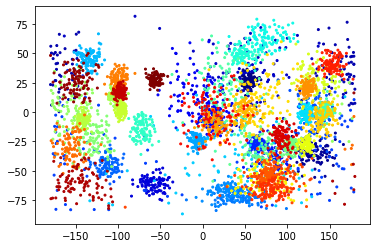
U1 dataset in 2D degree Space ($\kappa_{max}=16$)

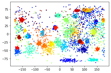
U2 dataset in 2D degree Space ($\kappa_{max}=32$)

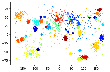
U3 dataset in 2D degree Space ($\kappa_{max}=64$)

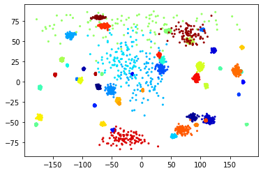
U4 dataset in 2D degree Space ($\kappa_{max}=128$)

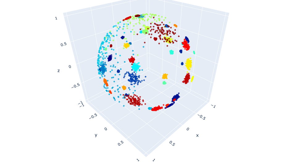
U4 dataset in 3D space ($\kappa_{max}=128$)

Figure 5: The data distributions of four synthetic datasets (U1, U2, U3, and U4) generated from the uniform sampling method. (e) shows the U4 dataset in a 3D Euclidean space. We can see that if we treat these datasets as 2D data points as $grid$ and $theory$, the $vMF$ distributions in the polar areas will be stretched and look like 2D aniostropic multivariate Gaussian distributions. However, this kind of systematic bias can be avoided if we use a spherical location encoder as $Sphere2Vec$.

S1.3 dataset in 2D degree Space ($N_{\mu}=5$)

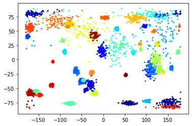
S2.3 dataset in 2D degree Space ($N_{\mu}=10$)

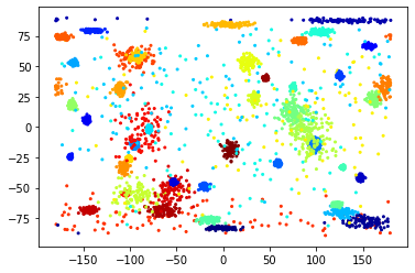
S3.3 dataset in 2D degree Space ($N_{\mu}=25$)

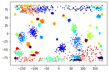
S4.3 dataset in 2D degree Space ($N_{\mu}=50$)

Figure 6: The data distributions of four synthetic datasets (S1.3, S2.3, S3.3, and S4.3) generated from the stratified sampling method with $\kappa_{max}=64$. We can see that when $N_{\mu}$ increases, a more fine-grain stratified sampling is carried out. The resulting dataset has a larger data bias toward the polar areas.

8 Experiments with Synthetic Datasets

Theorem 1 and 2 provide theoretical guarantees of Sphere2Vec for spherical distance preservation. To empirically verify the effectiveness of Sphere2Vec in a controlled setting, we construct a set of synthetic datasets and evaluate our Sphere2Vec and all baseline models on these datasets. To make a simpler task, different from the setting shown in Figure 1, we skip the image encoder component and only focus on the location encoder training and evaluation. For each synthetic dataset, we simulate a set of spherical coordinates as the geo-locations of images to train different location encoders. And in the evaluation step, the performances of different models are computed directly based on $P(y|\boldsymbol{\mathbf{x}})$ only, but not $P(y|\boldsymbol{\mathbf{x}})P(y|\mathbf{I})$.

8.1 Synthetic Dataset Generation

We utilize the von Mises–Fisher distribution ($vMF$) (Izbicki et al., 2019a), an analogy of the 2D Gaussian distribution on the spherical surface $\mathbb{S}^{2}$ to generate synthetic data points. The probability density function of $vMF$ is defined as

$$\begin{split}vMF(\boldsymbol{\mathbf{x}};\mu,\kappa)&=\dfrac{\kappa}{2\pi\sinh(\kappa)}\exp(\kappa\mu^{T}\chi(\boldsymbol{\mathbf{x}}))\end{split}$$ (24)

where $\chi(\boldsymbol{\mathbf{x}})=[x,y,z]=[\cos\phi\cos\lambda,\cos\phi\sin\lambda,\sin\phi]$, which converts $\boldsymbol{\mathbf{x}}$ into a coordinates in the 3D Euclidean space on the surface of a unit sphere. A $vMF$ distribution is controlled by two parameters – the mean direction $\mu\in\mathbb{R}^{3}$ and concentration parameter $\kappa\in\mathbb{R}^{+}$. $\mu$ indicates the center of a $vMF$ distribution which is a 3D unit vector. $\kappa$ is a positive real number which controls the concentration of $vMF$. A higher $\kappa$ indicates more compact $vMF$ distribution, while $\kappa=1$ correspond to a $vMF$ distribution with standard deviation covering half of the unit sphere.

To simulate multi-modal distributions, we generate spherical coordinates based on a mixture of von Mises–Fisher distributions (MvMF). We assume $\mathcal{C}$ classes with even prior, and each classes follows a $vMF$ distribution. To create a dataset we first sample $\mathcal{C}$ sets of parameters $\{(\mu_{i},\kappa_{i})\}$ ($\mathcal{C}=50$). Then we draw $\mathcal{SP}$ samples, i.e., spherical coordinates, for each class ($\mathcal{SP}=100$). So in total, each generated synthetic dataset has 5000 data points for 50 balanced classes.

The concentration parameter $\kappa_{i}$ is sampled by first drawing $r$ from an uniform distribtuion $U(\kappa_{min},\kappa_{max})$, and then take the square $r^{2}$. The square helps to avoid sampling many large $\kappa_{i}$ which yield very concentrated $vMF$ distributions that are rather easy to be classified. We fix $\kappa_{min}=1$ and vary $\kappa_{max}$ in $[16,32,64,128]$.

For the center parameter $\mu_{i}$ we adopt two sampling approaches:

1. Uniform Sampling: We uniformly sample $\mathcal{C}$ centers ($\mu_{i}$) from the surface of a unit sphere. We generate four synthetic datasets (for different values of $\kappa_{max}$) and indicate them as U1, U2, U3, U4. See Table 1 for the parameters we use to generate these datasets.

2. Stratified Sampling: We first evenly divide the latitude range $[-\pi/2,\pi/2]$ into $N_{\mu}$ intervals. Then we uniformly sample $\mathcal{C}_{\mu}$ centers ($\mu_{i}$) from the spherical surface defined by each latitude interval. Since the latitude intervals in polar regions have smaller spherical surface area, this stratified sampling method has higher density in the polar regions. We keep $N_{\mu}\times\mathcal{C}_{\mu}=\mathcal{C}=50$ fixed and varies $N_{\mu}$ in $[5,10,25,50]$. Combined with the 4 $\kappa_{max}$ choices, this procedure yields 16 different synthetic datasets. We denote them as $Si.j$. See Table 1 for the parameters we use to generate these datasets.

Figure 5-5 visualize the data point distributions of U1, U2, U3, U4 which derived from the uniform sampling method in 2D space. Figure 5 visualized the U4 dataset in a 3D Euclidean space. We can see that when $\kappa_{max}$ is larger, the variation of point density among different $vMF$ distributions becomes larger. Some $vMF$ are very concentrated and the resulting data points are easier to be classified. Moreover, if we treat these datasets as 2D data points as $grid$ and $theory$ do, $vMF$ distributions in the polar areas will be stretched to very extended shapes making model learning more difficult. However, this kind of systematic bias can be avoided if we use a spherical location encoder as Sphere2Vec.

Figure 6 visualizes the data distributions of four synthetic datasets with stratified sampling method. They have different $N_{\mu}$ but the same $\kappa_{max}$. We can see that when $N_{\mu}$ increases, a more fine-grain stratified sampling is carried out. The resulting dataset has a larger data bias toward the polar areas.

Table 1: Compare $sphereM+$ to baselines on synthetic datasets. We use Top1 as the evaluation metric. U1 - U4 indicate 4 synthetic datasets generated based on the uniform sampling approach (see Section 8.1). S1.1 - S4.4 indicate 16 synthetic datasets generated based on the stratified sampling apprach. For all datasets have $\mathcal{C}=50$ and $\mathcal{SP}=100$. For each model, we perform grid search on its hyperparameters for each dataset and report the best Top1 accuracy. The $\Delta Top1$ column shows the absolute performance improvement of $sphereM+$ over the best baseline model (bolded) for each dataset. The $ER$ column shows the relative reduction of error compared to the best baseline model (bolded). We can see that $sphereM+$ can outperform all other baseline models on all of these 20 synthetic datasets. The absolute Top1 accuracy improvement can be as much as 2.0% for datasets with lower precisions, and the error rate deduction can be as much as $30.8\%$ for datasets with high precisions.

ID	Method	$N_{\mu}$	$\mathcal{C}_{\mu}$	$\kappa_{min}$	$\kappa_{max}$	$xyz$	$wrap$	$wrap$+ffn	$rff$	$rbf$	$grid$	$theory$	$NeRF$	$sphereM+$	$\Delta Top1$	$ER$
U1	uniform	-	-	1	16	67.2	67.0	66.9	66.8	46.6	68.6	67.8	62.7	69.2	0.6	-1.9
U2					32	73.1	75.1	73.9	72.3	58.4	76.2	76.5	72.5	77.4	0.9	-3.8
U3					64	86.1	90.1	88.3	89.0	91.7	92.3	92.7	90.1	93.3	0.6	-8.2
U4					128	91.8	94.9	92.3	92.5	97.4	97.5	97.7	95.7	98.0	0.3	-13.0
S1.1	stratified	5	10	1	16	68.7	69.7	68.8	68.6	70.5	69.5	69.4	66.5	72.3	1.8	-6.1
S1.2					32	76.7	79.1	78.1	78.4	81.1	81.2	79.2	76.1	82.9	1.7	-9.0
S1.3					64	91.2	92.5	92.9	92.6	94.7	94.8	94.9	92.1	95.4	0.5	-9.8
S1.4					128	86.5	91.6	88.3	92.4	93.5	95.2	94.9	92.4	96.1	0.9	-18.7
S2.1		10	5	1	16	70.5	71.3	70.7	70.4	46.6	72.0	70.7	67.0	74.0	2.0	-7.1
S2.2					32	76.1	79.7	78.2	78.6	61.2	80.9	80.5	77.6	82.3	1.4	-7.3
S2.3					64	88.0	89.9	88.2	88.5	80.0	92.5	91.9	89.0	93.3	0.8	-10.7
S2.4					128	94.4	96.6	96.7	95.5	94.0	97.6	97.6	96.2	98.1	0.5	-20.8
S3.1		25	2	1	16	66.2	66.3	64.7	65.6	67.1	66.7	66.7	61.3	68.3	1.2	-3.6
S3.2					32	80	82.5	80.7	81.6	83.4	84.5	82.1	80.3	85.9	1.4	-9.0
S3.3					64	85.4	86.0	85.7	86.2	89.1	89.6	88.6	86.1	91.0	1.4	-13.5
S3.4					128	93.2	96.0	94.8	95.7	97.2	97.3	97.4	96.7	98.0	0.6	-23.1
S4.1		50	1	1	16	64.8	67.4	66.0	66.3	66.9	67.1	64.5	62.9	68.4	1	-3.1
S4.2					32	75.6	78.2	77.4	77.4	78.4	80.1	78.3	75.7	81.0	0.9	-4.5
S4.3					64	91.3	93.9	93.7	93.8	95.0	95.2	94.0	92.5	96.1	0.9	-18.7
S4.4					128	94.3	95.5	94.4	94.7	95.4	97.4	96.5	95.2	98.2	0.8	-30.8

8.2 Synthetic Dataset Evaluation Results

We evaluate all baseline models as well as $sphereM+$ on those generated 20 syhthetic datasets as described above. For each model, we do grid search on their hyperparameters for each dataset including supervised learning rate $lr$, the number of scales $S$, the minimum scaling factor $r_{min}$, the number of hidden layers and number of neurons used in $\mathbf{NN}^{ffn}(\cdot)$ – $h$ and $k$. The best performance of each model is reported in Table 1. We use Top1 as the evaluation metric. The Topk classification accuracy is defined as follow

$$TOP_{k}=\dfrac{1}{|\mathcal{M}|}\sum_{i=1}^{|\mathcal{M}|}\mathbf{1}(Rank(\boldsymbol{\mathbf{x}}_{i},y_{i})\geqslant k)$$ (25)

where $\mathcal{M}=\{(\boldsymbol{\mathbf{x}}_{i},y_{i})\}$ is a set of location $\boldsymbol{\mathbf{x}}_{i}$ and label $y_{i}$ tuples which indicates the whole validation or testing set. $|\mathcal{M}|$ denotes the total number of samples in $\mathcal{M}$. $Rank(\boldsymbol{\mathbf{x}}_{i},y_{i})$ indicates the rank of the ground truth label $y_{i}$ in the ranked listed of all classes based on the probability score $P(y_{i}|\boldsymbol{\mathbf{x}}_{i})$ given by a specific location encoder. A lower rank indicates a better model prediction. $\mathbf{1}(*)$ is a function return 1 when the condition $*$ is true and 0 otherwise. A higher Topk indicates a better performance.

Some observations can be made from Table 1:

1. $sphereM+$ is able to outperform all baselines on all 20 synthetic datasets. The absolute Top1 improvement can go up to 2% and the error rate deduction can go up to $30.8\%$. This shows the robustness of $sphereM+$.

2. When the dataset is fairly easy to classify (i.e., all baseline models can produce 95+% Top1 accuracy), $sphereM+$ is still able to further improve the performance and gives a very large error rate reduction (up to 30.8%). This indicates that $sphereM+$ is very robust and reliable for datasets with different distribution characteristics.

3. Comparing the error rate of different stratified sampling generated datasets (S1.j - S4.j) we can see that when we keep $\kappa_{max}$ fixed and increase $N_{\mu}$, the relative error reduction $ER$ become larger. Increasing $N_{\mu}$ means we do a more fine-grain stratified sampling. The resulting datasets should sample more $vMF$ distributions in the polar regions. This phenomenon shows that when the dataset has a larger data bias towards the polar area, we expect $sphereM+$ to be more effective.

4. From Table 1, we can also see that among all the baseline methods, $grid$ achieves the best performances on most datasets (12 out of 20), followed by $theory$ (5 out of 20). This observation aligns the experiment results from Mai et al. (2020b) which shows the advantages of multiscale location representation versus single-scale representations.

5. It is interesting to see that although $NeRF$ is also a multiscale location encoding approach, it underperforms $grid$ and $theory$ on all synthetic datasets. We guess the reasons are 1) $NeRF$ treats geo-coordinates as 3D Euclidean coordinates and ignores the fact that they are all on the spherical surface which yields more modeling freedom and makes it more difficult for $\mathbf{NN}^{ffn}$ to learn; 2) $NeRF$ uses predefined Fourier scales, i.e., $\{2^{0},2^{1},...,2^{s},...,2^{S-1}\}$, while $grid$, $theory$, and $Sphere2Vec$ are more flexible in terms of Fourier scale choices which are controlled by $r_{max}$ and $r_{min}$.

9 Experiment with Geo-Aware Image Classification

Next, we empirically evaluate the performances of our Sphere2Vec as well as all 9 baseline methods on 7 real-world datasets for the geo-aware image classification task.

9.1 Dataset

More specifically, we test the performances of different location encoders on seven datasets from three different problems: fine-grained species recognition, Flickr image recognition, and remote sensing image classification. The statistics of these seven datasets are shown in Table 2. Figure 7 and 8 show the spatial distributions of the training, validation/testing data of these datasets.

Table 2: Dataset statistics on different geo-aware image classification datasets. "Train", "Val", and "Test" column indicates the number of data samples in each dataset. "#Class" column indicates the total number of classes for each dataset.

Task	Dataset	Train	Val	Test	#Class
Species Recog.	BirdSnap	19133	443	443	500
	BirdSnap†	42490	980	980	500
	NABirds†	22599	1100	1100	555
	iNat2017	569465	93622	-	5089
	iNat2018	436063	24343	-	8142
Flickr	YFCC	66739	4449	4449	100
RS	fMoW	363570	53040	-	62

Fine-Grained Species Recognition

We use five widely used fine-grained species recognition image datasets in which each data sample is a tuple of an image $\mathbf{I}$, a location $\boldsymbol{\mathbf{x}}$, and its ground truth class $y$:

1. BirdSnap: An image dataset about bird species based on BirdSnap dataset (Berg et al., 2014) which consists of 500 bird species that are commonly found in the North America. The original BirdSnap dataset (Berg et al., 2014) did not provided the location metadata. Mac Aodha et al. (2019) recollected the images and location data based on the original image URLs.

2. BirdSnap†: An enriched BirdSnap dataset constructed by Mac Aodha et al. (2019) by simulating locations, dates, and photographers from the eBrid dataset (Sullivan et al., 2009).

3. NABirds†: Another image dataset about North American bird species constructed by Mac Aodha et al. (2019) based on the NABirds dataset (Van Horn et al., 2015) in which the location metadata were also simulated from the eBrid dataset (Sullivan et al., 2009).

4. iNat2017: The species recognition dataset used in the iNaturalist 2017 challenges (Van Horn et al., 2018) with 5089 unique categories.

5. iNat2018: The species recognition dataset used in the iNaturalist 2018 challenges (Van Horn et al., 2018) with 8142 unique categories.

Flickr Image Classification

We use the Yahoo Flickr Creative Commons 100M dataset (YFCC100M-GEO100 dataset) which is a set of geo-tagged Flickr photos collected by Yahoo! Research. Here, we denote this dataset as YFCC. YFCC has been used in Tang et al. (2015); Mac Aodha et al. (2019) for geo-aware image classification. See Figure 8 and 8 for the spatial distributions of the training and test dataset of YFCC.

Remote Sensing Image Classification

We use the Functional Map of the World dataset (denoted as fMoW) (Klocek et al., 2019) as one representative remote sensing (RS) image classification dataset. The fMoW dataset contains about 363K training and 53K validation remote sensing images which are classfied into 62 different land use types. They are 4-band or 8-band multispectral remote sensing images. 4-band images are collected from the QuickBird-2 or GeoEye-1 satellite systems while 8-band images are from WorldView-2 or WorldView-3. We use the fMoW-rgb version of fMoW dataset which are JPEG compressed version of these remote sensing images with only the RGB bands. The reason we pick fMoM is that 1) the fMoW dataset contains RS images with diverse land use types collected all over the world (see Figure 8 and 8); 2) it is a large RS image dataset with location metadata available. In contrast, the UC Merced dataset (Yang and Newsam, 2010) consist of RS images collected from only 20 US cities. The EuroSAT dataset (Helber et al., 2019) contained RS images collected from 30 European countries. And the location metadata of the RS images from these two datasets are not publicly available. Global coverage of the RS images is important in our experiment since we focus on studying how the map projection distortion problem and spherical-to-Euclidean distance approximation error can be solved by Sphere2Vec on a global scale geospatial problem. The reason we use the RGB version is that this dataset version has an existing pretrained image encoder – MoCo-V2+TP (Ayush et al., 2020) available to use. We do not need to train our own remote sensing image encoder.

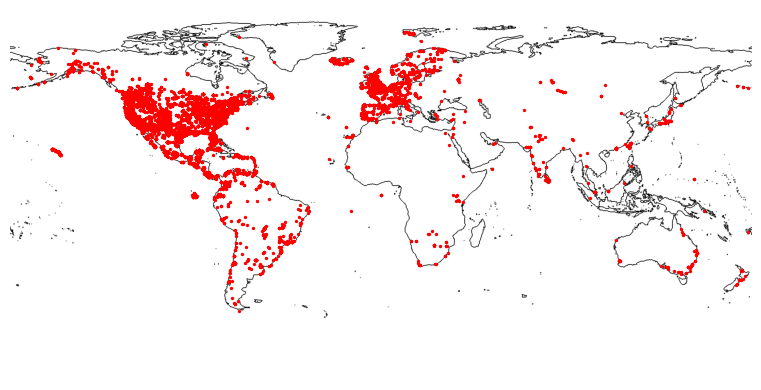
BirdSnap Train

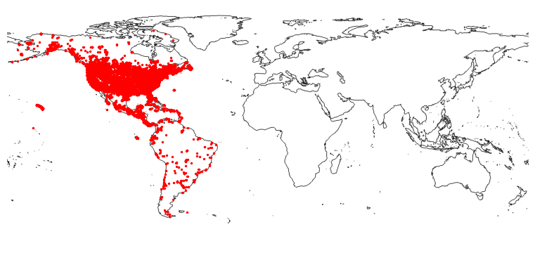
BirdSnap† Train

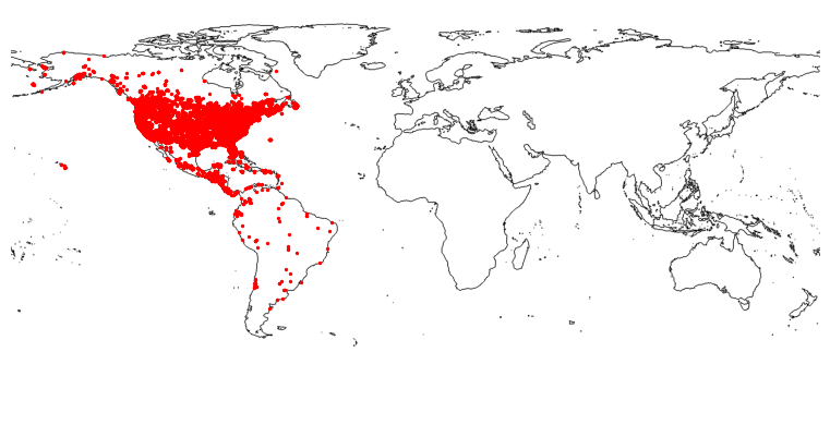
NABirds† Train

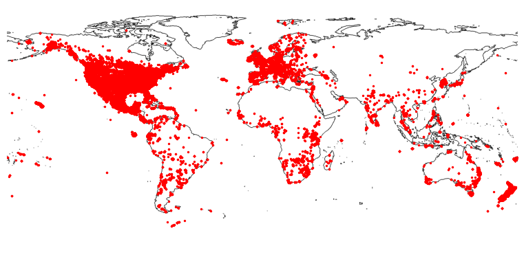
iNat2017 Train

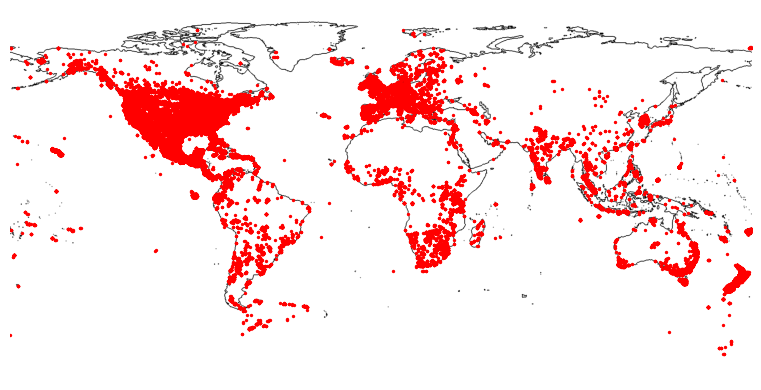
iNat2018 Train

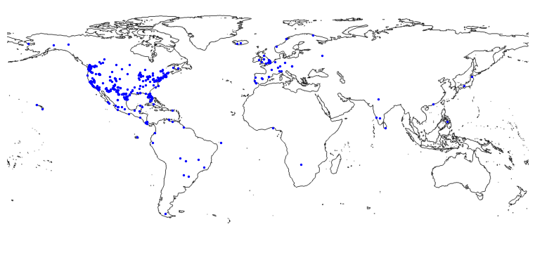
BirdSnap Test

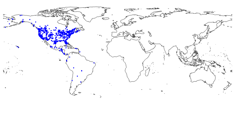
BirdSnap† Test

NABirds† Test

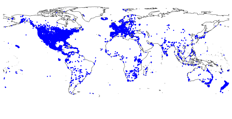
iNat2017 Val

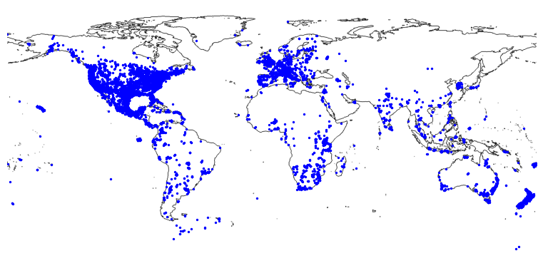
iNat2018 Val

Figure 7: Training, validation/testing locations of different fine-grained species recognition datasets. Different datasets use either validation or testing dataset to evaluate model performance. So we plot their corresponding image geographic distributions.

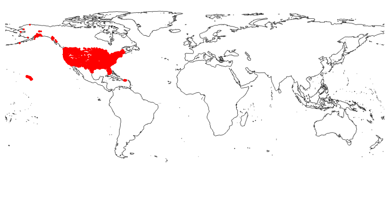
YFCC Train

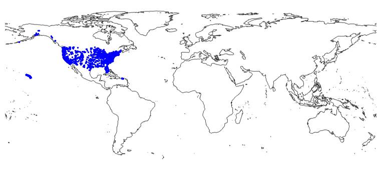
YFCC Test

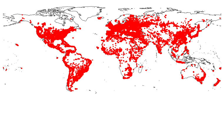
fMoW Train

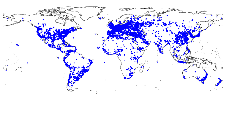
fMoW Val

Figure 8: Training and validation/testing locations of Flickr image recognition (YFCC) and RS image classification (fMoW).

9.2 Geo-Aware Image Classification

Table 3: The Top1 classification accuracy of different geo-aware image classification models over three tasks: species recognition, Flickr image classification (YFCC), and remote sensing (RS) image classification (fMOW (Christie et al., 2018)). See Section 6 for the description of each baseline. $tile$ indicates the results reported by Mac Aodha et al. (2019). $wrap*$ indicates the original results reported by Mac Aodha et al. (2019) while $wrap$ is the best results we obtained by rerunning their code. Since the test sets for iNat2017, iNat2018, and fMoW are not open-sourced, we report results on validation sets. The best performance of the baseline models and Sphere2Vec are highlighted as bold. All compared models use location only while ignoring time. The original result reported by Ayush et al. (2020) for No Prior on fMOW is 69.05. We obtain 69.84 by retraining their implementation. "Avg" column indicates the average performance of each model on all five species recognition datasets. See Section 9.3 for hyperparameter tuning details.

Task	Species Recognition						Flickr	RS
Dataset	BirdSnap	BirdSnap†	NABirds†	iNat2017	iNat2018	Avg	YFCC	fMOW
P(y|x) - Prior Type	Test	Test	Test	Val	Val	-	Test	Val
No Prior (i.e. image model)	70.07	70.07	76.08	63.27	60.20	67.94	50.15	69.84
$tile$ (Tang et al., 2015)	70.16	72.33	77.34	66.15	65.61	70.32	50.43	-
$xyz$	71.85	78.97	81.20	69.39	71.75	74.63	50.75	70.18
$wrap*$ (Mac Aodha et al., 2019)	71.66	78.65	81.15	69.34	72.41	74.64	50.70	-
$wrap$	71.87	79.06	81.62	69.22	72.92	74.94	50.90	70.29
$wrap+ffn$	71.99	79.21	81.36	69.40	71.95	74.78	50.76	70.28
$rbf$(Mai et al., 2020b)	71.78	79.40	81.32	68.52	71.35	74.47	51.09	70.65
$rff$(Rahimi et al., 2007)	71.92	79.16	81.30	69.36	71.80	74.71	50.67	70.27
Space2Vec-$grid$ (Mai et al., 2020b)	71.70	79.72	81.24	69.46	73.02	75.03	51.18	70.80
Space2Vec-$theory$ (Mai et al., 2020b)	71.88	79.75	81.30	69.47	73.03	75.09	51.16	70.81
$NeRF$ (Mildenhall et al., 2020)	71.66	79.66	81.32	69.45	73.00	75.02	50.97	70.64
Sphere2Vec-$sphereC$	72.11	79.80	81.88	69.68	73.29	75.35	51.34	71.00
Sphere2Vec-$sphereC+$	72.41	80.11	81.97	69.75	73.31	75.51	51.28	71.03
Sphere2Vec-$sphereM$	72.06	79.84	81.94	69.72	73.25	75.36	51.35	70.99
Sphere2Vec-$sphereM+$	72.24	80.57	81.94	69.67	73.80	75.64	51.24	71.10
Sphere2Vec-$dfs$	71.75	79.18	81.39	69.65	73.24	75.04	51.15	71.46

To test the effectiveness of Sphere2Vec, we conduct geo-aware image classification experiments on seven large-scale real-world datasets as we described in Section 9.1.

Beside the baselines described in Section 6, we also consider $No\;Prior$, which represents an full supervised trained image classifier without using any location information, i.e., predicting image labels purely based on image information $P(y|\mathbf{I})$.

Table 3 compares the Top1 classification accuracy of five variants of Sphere2Vec models against those of nine baseline models as we discussed in Section 6.

Similar to Equation 25, the Topk classification accuracy on geo-aware image classification task is defined as follow

$$TOP_{k}=\dfrac{1}{|\mathcal{M}|}\sum_{i=1}^{|\mathcal{M}|}\mathbf{1}(Rank(\boldsymbol{\mathbf{x}}_{i},\mathbf{I}_{i},y_{i})\geqslant k)$$ (26)

where $\mathcal{M}=\{(\boldsymbol{\mathbf{x}}_{i},\mathbf{I}_{i},y_{i})\}$ is a set of location $\boldsymbol{\mathbf{x}}_{i}$, image $\mathbf{I}_{i}$, and label $y_{i}$ tuples which indicates the whole validation or testing set. $|\mathcal{M}|$ denotes the total number of samples in $\mathcal{M}$. $Rank(\boldsymbol{\mathbf{x}}_{i},\mathbf{I}_{i},y_{i})$ indicates the rank of the ground truth label $y_{i}$ in the ranked listed of all classes based on the probability score $P(y_{i}|\boldsymbol{\mathbf{x}}_{i})P(y_{i}|\mathbf{I}_{i})$ given by a specific geo-aware image classification model. $\mathbf{1}(*)$ is defined the same as that in Equation 25.

From Table 3, we can see that the Sphere2Vec models outperform baselines on all seven datasets, and the variants with linear number of DFS terms ($sphereC$, $sphereC+$, $sphereM$, and $sphereM+$) works as well as or even better than $dfs$. This clearly show the advantages of Sphere2Vec to handle large-scale geographic datasets. On the five species recognition datasets, $sphereM+$ achieves the best performance while $sphereM$ and $dfs$ achieve the best performance on YFCC and fMoW correspondingly. Similar to our findings in the synthetic dataset experiments, $grid$ and $theory$ also outperform or are comaprable to $NeRF$ on all 7 real-world datasets.

9.3 Hyperparameter Analysis

In order to find the best hyperparameter combinations for each model on each dataset, we use grid search to do hyperparameter tuning including supervised training learning rate $lr=[0.01,0.005,0.002,0.001,0.0005,0.00005]$, the number of scales $S=[16,32,64]$, the minimum scaling factor $r_{min}=[0.10.050.020.010.0050.0010.0001]$, the number of hidden layers and number of neurons used in $\mathbf{NN}^{ffn}(\cdot)$ – $h=[1,2,3,4]$ and $k=[256,512,1024]$, the dropout rate in $\mathbf{NN}^{ffn}(\cdot)$ – $dropout=[0.1,0.2,0.3,0.4,0.5,0.6,0.7]$. We also test multiple options for the nonlinear function used for $\mathbf{NN}^{ffn}(\cdot)$ including ReLU, LeakyReLU, and Sigmoid. The maximum scaling factor $r_{max}$ can be determined based on the range of latitude $\phi$ and longitude $\lambda$. For $grid$ and $theory$, we use $r_{max}=360$ and for all Sphere2Vec, we use $r_{max}=1$. As for $rbf$ and $rff$, we also tune their hyperparamaters including kernel size $\sigma=[0.5,1,2,10]$ as well as the number of kernels $M=[100,200,500]$.

Based on hyperparameter tuning, we find out using 0.5 as the dropout rate and ReLU as the nonlinear activation function for $\mathbf{NN}^{ffn}(\cdot)$ works best for every location encoder. Moreover, we find out $lr$ and $r_{min}$ are the most important hyperparameters. Table 4 shows the best hyperparameter combinations of different Sphere2Vec models on different geo-aware image classification datasets. We use a smaller $S$ for $dfs$ since it has $O(S^{2})$ terms while the other models have $O(S)$ terms. $dfs$ with $S=8$ yield a similar number of terms to the other models with $S=32$ (see Table 5). Interestingly, all five Sphere2Vec models ($sphereC$, $sphereC+$, $sphereM$, $sphereM+$, and $dfs$) show the best performance on the first six datasets with the same hyperparamter combinations. On the fMoW dataset, five Sphere2Vec achieve the best performances with different $r_{min}$ but sharing other hyperparameters. This indicates that the proposed Sphere2Vec models show similar performance over different hyperparameter combinations.

Table 4: The best hyperparameter combinations of Sphere2Vec models on different geo-aware image classification datasets. The best $S$ is 8 for $dfs$ and 32 for all others; and we fix the maximum scale $r_{max}$ as 1. Here, $r_{min}$ indicates the minimum scale. $h$ and $k$ are the number of hidden layers and the number of neurons in $\mathbf{NN}()$ respectively.

Dataset	Model	$lr$	$r_{min}$	$k$
BirdSnap	All	0.001	$10^{-6}$	512
BirdSnap$\dagger$	All	0.001	$10^{-4}$	1024
NABirds$\dagger$	All	0.001	$10^{-4}$	1024
iNat2017	All	0.0001	$10^{-2}$	1024
iNat2018	All	0.0005	$10^{-3}$	1024
YFCC	All	0.001	$5\times 10^{-3}$	512
fMoW	sphereC	0.01	$10^{-3}$	512
	sphereC+		$10^{-4}$
	sphereM		$10^{-3}$
	sphereM+		$5\times 10^{-4}$
	dfs		$10^{-4}$

Table 5: Dimension of position encoding for different models in terms of total scales $S$

Model	$sphereC$	$sphereC+$	$sphereM$	$sphereM+$	$dfs$
Dim.	$3S$	$6S$	$5S$	$8S$	$4S^{2}+4S$

We also find out that using a deeper MLP as $\mathbf{NN}^{ffn}(\cdot)$, i.e., a larger $h$ does not necessarily lead to better classification accuracy. In many cases, one hidden layer – $h=1$ achieves the best performance for many kinds of location encoders. We discuss this in detail in Section 9.4.2.

Based on the hyperparameter tuning, the best hyperparameter combinations are selected for different models on different datasets. The best results are reported in Table 3. Note that each model has been running for 5 times and its mean Top1 score is reported. Due to the limit of space, the standard deviation of each model’s performance on each dataset is not included in Table 3. However, we report the standard deviations of all models’ performance on three datasets in Section 9.4.2.

9.4 Model Performance Sensitivity Analysis

9.4.1 Model Performance Distribution Comparison

To have a better understanding of the performance difference between Sphere2Vec and all baseline models, we visualize the distributions/histograms of Top1 accuracy scores of different models on the BirdSnap†, NABirds†, iNat2018, and YFCC dataset under different hyperparameter combinations. More specifically, after the hyperparameter tuning process described in Section 9.3, for each location encoder and each dataset we get a collection of trained models with different hyperparameter combinations. They correspond to a distribution/histograms of Top1 accuracy scores for this model on the respective dataset. Figure 9 compares the histogram of $sphereM+$ and all baseline models on four datasets. We can see that the histogram of $sphereM+$ is clearly above those of all baselines. This further demonstrates the superiority of Sphere2Vec over all baselines.

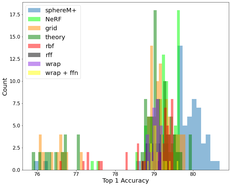
BirdSnap† dataset

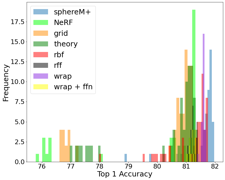
NABirds† dataset

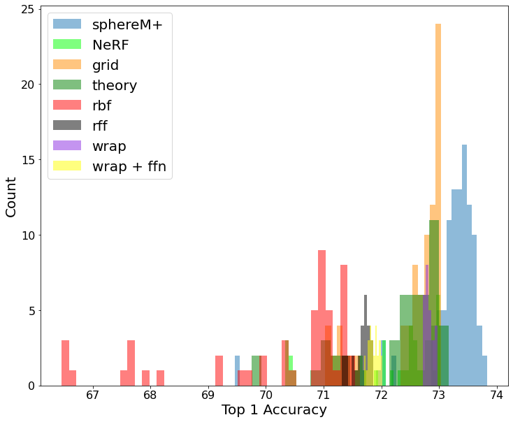
iNat2018 dataset

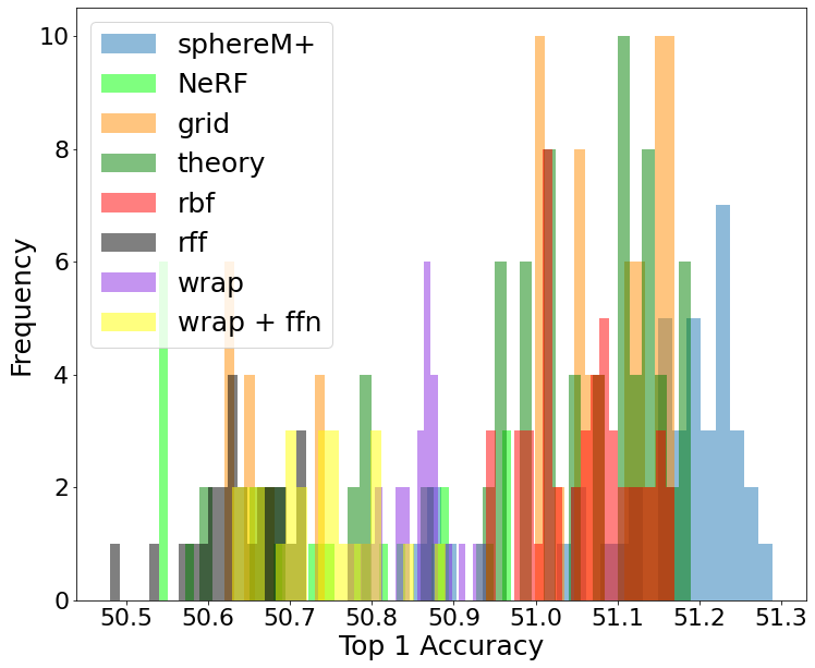
YFCC dataset

Figure 9: The model performance (Top1 accuracy) distributions/histograms of different models under different hyperparameter combinations on (a) the BirdSnap† dataset, (b) the NABirds† dataset, (c) the iNat2018 dataset, and (d) the YFCC dataset. X axis: the Top1 accuracy scores of the respective model; Y axis: the frequency of different hyperparameter combinations of the same model falling in the same Top1 Accuracy bin. In all four plots, each color indicate a Top1 accuracy histogram of one specific model on a specific dataset. This histogram shows the model’s sensitivity towards different hyperparameter combinations. We can see that in all four plots, the histogram of $sphereM+$ (the blue histogram) are clearly different from all baseline models’ histograms. This shows the clear advantage of $sphereM+$ over all baselines.

9.4.2 Performance Sensitivity to the Depth of MLP

To further understand how the performances of different location encoders vary according to the depth of the multi-layer perceptron $\mathbf{NN}^{ffn}()$, we conduct a performance sensitivity analysis. Table 6 is a complementary of Table 3 which compares the performance of $sphereM+$ with all baseline models on the geo-aware image classification task. The results on three datasets are shown here including BirdSnap†, NABirds†, and iNat2018. For each model, we vary the depth of its $\mathbf{NN}^{ffn}()$, i.e., $h=[1,2,3,4]$. The best evaluation results with each $h$ are reported. Moreover, we run each model with one specific $h$ 5 times and report the standard deviation of the Top1 accuray, indicated in “()”. Several observations can be made based on Table 6:

1. Although the absolute performance improvement between $sphereM+$ and the best baseline model is not very large – 0.91%, 0.62%, and 0.77% for three datasets respectively, these performance improvements are statistically significant given the standard deviations of these Top1 scores.

2. These performance improvements are comparable to those from the previous studies on the same tasks. In other words, the small margin is due to the nature of these datasets. For example, Mai et al. (2020b) showed that $grid$ or $theory$ has 0.79%, 0.44% absolute Top1 accuracy improvement on BirdSnap† and NABirds† dataset respectively. Mac Aodha et al. (2019) showed that $wrap$ has 0.09%, 0%, 0.04% absolute Top1 accuracy improvement on BirdSnap, BirdSnap† and NABirds† dataset. Here, we only consider the results of $wrap$ that only uses location information, but not temporal information. Although Mac Aodha et al. (2019) showed that compared with $tile$ and nearest neighbor methods, $wrap$ has 3.19% and 3.71% performance improvement on iNat2017 and iNat2018 datatset, these large margins are mainly because the baselines they used are rather weak. When we consider the typical $rbf$ and $rff$ (Rahimi et al., 2007) used in our study, their performance improvements are down to -0.02% and 0.61%.

3. By comparing the performances of the same model with different depths of its $\mathbf{NN}^{ffn}()$, i.e., $h$, we can see that the model performance is not sensitive to $h$. In fact, in most cases, one layer $\mathbf{NN}^{ffn}()$ achieves the best result. This indicates that the depth of the MLP does not significantly affect the model performance and a deeper MLP does not necessarily lead to a better performance. In other words, the systematic bias (i.e., distance distortion) introduced by $grid$, $theory$, and $NeRF$ can not later be compensated by a deep MLP. It shows the importance of designing a spherical-distance-aware location encoder.

Table 6: The impact of the depth $h$ of multi-layer perceptrons $\mathbf{NN}^{ffn}()$ on Top1 accuracy for various models. The numbers in “()” indicates the standard deviations estimated from 5 independent train/test runs. We find that the model performances are not very sensitive to $\mathbf{NN}^{ffn}()$, and, in most cases, one layer $\mathbf{NN}^{ffn}()$ achieve the best result. In other words, the larger performance gaps in fact come from different $PE_{S}(\cdot)$ we use. Moreover, given the performance variance of each model, we can see that $sphereM+$ outperforms other baseline models on all these three datasets and the margins are statistically significant. The same conclusion can be drawn based on our experiments on other datasets. Here, we only show results on three datasets as an illustrative example.

Dataset		BirdSnap†	NABirds†	iNat2018
	$h$	Test	Test	Val
$xyz$	1	78.81 (0.10)	81.08 (0.05)	71.60 (0.08)
	2	78.83 (0.10)	81.20 (0.09)	71.70 (0.02)
	3	78.97 (0.06)	81.11 (0.06)	71.75 (0.04)
	4	78.84 (0.09)	81.02 (0.03)	71.71 (0.03)
$wrap$	1	79.04 (0.13)	81.60 (0.04)	72.89 (0.08)
	2	78.94 (0.13)	81.62 (0.04)	72.84 (0.07)
	3	79.08 (0.15)	81.53 (0.02)	72.92 (0.05)
	4	79.06 (0.11)	81.51 (0.09)	72.77 (0.06)
$wrap+ffn$	1	78.97 (0.09)	81.23 (0.06)	71.90 (0.05)
	2	79.02 (0.15)	81.36 (0.04)	71.95 (0.05)
	3	79.21 (0.14)	81.35 (0.05)	71.94 (0.04)
	4	79.06 (0.09)	81.27 (0.13)	71.93 (0.04)
$rbf$	1	79.40 (0.13)	81.32 (0.08)	71.02 (0.18)
	2	79.38 (0.12)	81.22 (0.11)	71.29 (0.20)
	3	79.40 (0.04)	81.31 (0.07)	71.35 (0.21)
	4	79.25 (0.05)	81.30 (0.07)	71.21 (0.19)
$rff$	1	78.96 (0.18)	81.27 (0.07)	71.76 (0.06)
	2	78.97 (0.04)	81.28 (0.05)	71.71 (0.09)
	3	79.07 (0.12)	81.30 (0.11)	71.80 (0.04)
	4	79.16 (0.13)	81.22 (0.11)	71.46 (0.05)
$grid$	1	79.72 (0.07)	81.24 (0.06)	73.02 (0.02)
	2	79.05 (0.06)	81.09 (0.07)	72.87 (0.05)
	3	79.23 (0.12)	80.95 (0.14)	72.69 (0.05)
	4	78.97 (0.10)	80.71 (0.10)	72.51 (0.07)
$theory$	1	79.75 (0.17)	81.23 (0.02)	73.03 (0.09)
	2	79.08 (0.20)	81.30 (0.11)	72.70 (0.02)
	3	78.94 (0.19)	81.00 (0.09)	72.49 (0.08)
	4	79.07 (0.14)	80.64 (0.14)	72.35 (0.07)
$NeRF$	1	79.66 (0.00)	81.27 (0.00)	73.00 (0.01)
	2	79.65 (0.02)	81.29 (0.00)	72.97 (0.03)
	3	79.40 (0.05)	81.32 (0.01)	72.88 (0.02)
4	79.24 (0.04)	81.23 (0.00)	72.80 (0.02)
$sphereM+$	1	80.57 (0.08)	81.87 (0.02)	73.80 (0.05)
	2	79.82 (0.14)	81.83 (0.04)	73.42 (0.06)
	3	80.03 (0.08)	81.94 (0.04)	73.40 (0.05)
	4	79.90 (0.15)	81.84 (0.09)	73.20 (0.04)

9.4.3 Ablation Studies on Approaches for Image and Location Fusion

Table 7: Ablation Studies on different ways to combine image and location information on the iNat2018 dataset. “Fusion” column indicates different methods to fuse image and location information. “$\mathbf{F}(\cdot)$” and “$Enc(\cdot)$” indicates the type of image encoder and location encoder used for each model. “$\mathbf{F}(\cdot)$ Train” denotes different ways to train the image encoder. “Frozen” means we use an InceptionV3 network pre-trained on ImageNet as an image feature extractor and freeze its learnable parameters while only finetuning the last softmax layer. “Finetune” means we finetune the whole image encoder $\mathbf{F}(\cdot)$.

Model	Concat (Frozen)	Concat (Finetune)	Post Fusion
$\mathbf{F}(\cdot)$	InceptionV3	InceptionV3	InceptionV3
$\mathbf{F}(\cdot)$ Train	Frozen	Finetune	Finetune
$Enc(\cdot)$	$sphereM+$	$sphereM+$	$sphereM+$
Top1	48.74	73.35	73.72

In Section 5.2, we discuss how we fusion the predictions from the image encoder and location encoder together for the final model prediction. However, there are other ways to fuse the image and location information. In this section, we conduct ablation studies on different image and location fusion approaches:

• Post Fusion is the method we adopt from Mac Aodha et al. (2019) which is illustrated in Figure 1. The image encoder $\mathbf{F}(\cdot)$ and location encoder $Enc(\cdot)$ are trained separately and their final predictions are combined.

• Concat (Img. Finetune) indicates a method in which the image embedding $\mathbf{F}(\mathbf{I})$ and the location embedding $Enc(\boldsymbol{\mathbf{x}})$ are concatenated together and fed into a softmax layer for the final prediction. The whole architecture is trained end-to-end.

• Concat (Img. Frozen) indicates the same model architecture as Concat (Img. Finetune). The only difference is that $\mathbf{F}(\cdot)$ is initialized by a pretrained weight and its learnable parameters are frozen during the image and location join training.

We conduct experiments on iNat2018 dataset and the results are shown in Table 7. We can see that:

• Post Fusion, the method we adopt in our study, achieves the best Top1 score and outperforms both Concat approaches. This result is aligned with the results of Chu et al. (2019).

• Concat (Img. Frozen) shows a significantly lower performance than Concat (Img. Finetune). This is understandable and consistent with the existing literature (Ayush et al., 2020) since the linear probing method, Concat (Img. Frozen), usually underperforms a fully fine-tuning method, Concat (Img. Finetune).

• Although Post Fusion only shows a small margin over Concat (Img. Finetune), the training process of Post Fusion is much easier since we can separate the training process of the image encoder $\mathbf{F}(\cdot)$ and location encoder $Enc(\cdot)$. In contrast, Concat (Img. Finetune) has to train a large network which is hard to do hyperparameter tuning.

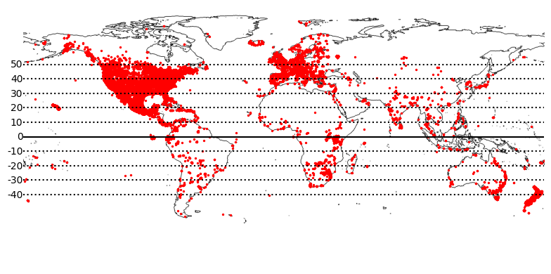
Validation Locations

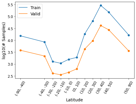
Samples per $\phi$ band

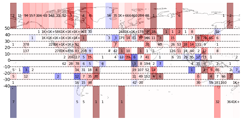
$\Delta MRR$ per cell

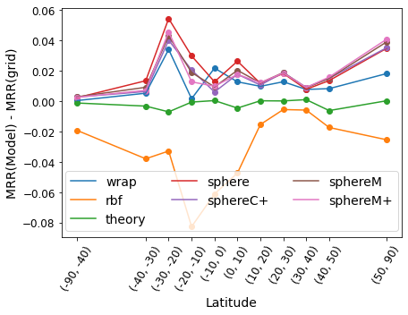
$\Delta MRR$ per $\phi$ band

Figure 10: The data distribution of the iNat2017 dataset and model performance comparison on it: (a) Sample locations for validation set of the iNat2017 dataset where the dashed and solid lines indicates latitudes; (b) The number of training and validation samples in different latitude intervals. (c) $\Delta MRR=MRR(sphereC+)-MRR(grid)$ for each latitude-longitude cell. Red and blue color indicates positive and negative $\Delta MRR$ while darker color means high absolute value. The number on each cell indicates the number of validation data points while "1K+" means there are more than 1K points in a cell. (d) $\Delta MRR$ between a model and baseline $grid$ on the validation dataset in different latitude bands.

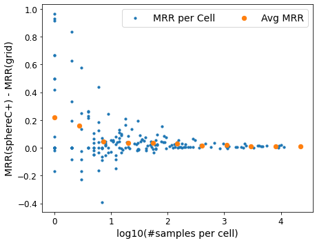
$\Delta MRR$ per cell

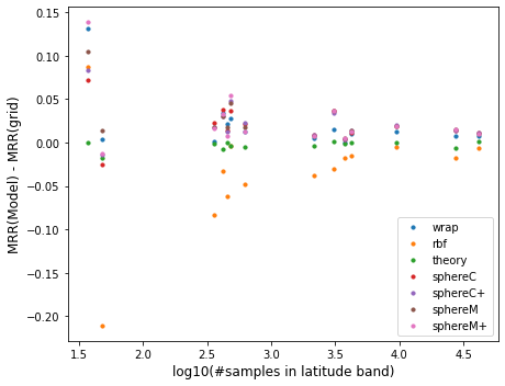
$\Delta MRR$ per $\phi$ band

Figure 11: The number of sample v.s. the model performance improvements on the iNat2017 dataset: (a) The number of validation samples v.s. $\Delta MRR=MRR($sphereC+) - MRR($grid)$ per latitude-longitude cell defined in Figure 10. The orange dots represent moving averages. (b) The number of validation samples v.s. $\Delta MRR$ per latitude band defined in Figure 10.

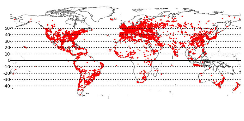
Validation Locations

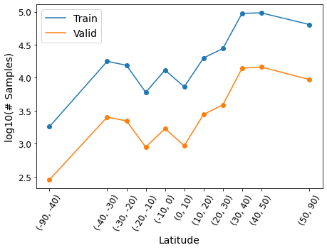
Samples per $\phi$ band

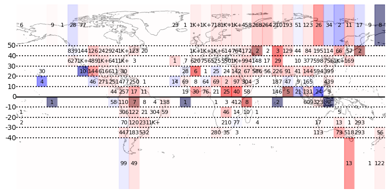
$\Delta MRR$ per cell

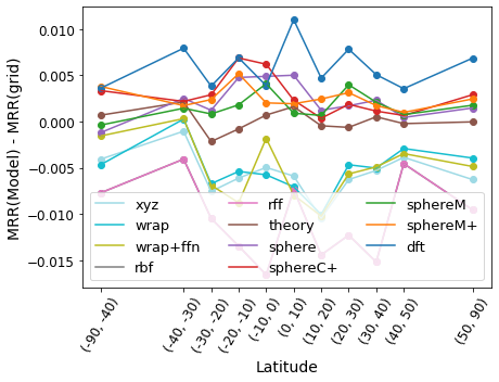
$\Delta MRR$ per $\phi$ band

Figure 12: The data distribution of the fMoW dataset and model performance comparison on it: (a) Sample locations for validation set of the fMoW dataset; (b) The number of training and validation samples in different latitude intervals. (c) $\Delta MRR=MRR(dfs)-MRR(grid)$ for each latitude-longitude cell. Red and blue color indicates positive and negative $\Delta MRR$ while darker color means high absolute value. The number on each cell indicates the number of validation data points while "1K+" means there are more than 1K points in a cell. (d) $\Delta MRR$ between a model and baseline $grid$ on the validation dataset in different latitude bands.

9.5 Understand the Superiority of Sphere2Vec

Based on the theoretical analysis of Sphere2Vec in Section A, we make two hypotheses to explain the superiority of Sphere2Vec over 2D Euclidean location encoders such as $theory$, $grid$:

• Our spherical-distance-kept Sphere2Vec have a significant advantage over 2D location encoders in the polar area where we expect a large map projection distortion.

• Sphere2Vec outperforms 2D location encoders in areas with sparse sample points because it is difficult for $grid$ and $theory$ to learn spherical distances in these areas with less samples but Sphere2Vec can handle it due to its theoretical guarantee for spherical distance preservation.

To validate these two hypotheses, we use iNat2017 and fMoW to conduct multiple empirical analyses. Table 3 uses Top1 classification accuracy as the evaluation metric to be aligned with several previous works (Mac Aodha et al., 2019; Mai et al., 2020b; Ayush et al., 2020). However, Top1 only considers the samples whose ground truth labels are top-ranked while ignoring all the other samples’ ranks. In contrast, mean reciprocal rank (MRR) considers the ranks of all samples. Equation 27 shows the definition of MRR:

$$MRR=\dfrac{1}{|\mathcal{M}|}\sum_{i=1}^{|\mathcal{M}|}\dfrac{1}{Rank(\boldsymbol{\mathbf{x}}_{i},\mathbf{I}_{i},y_{i})}.$$ (27)

where $|\mathcal{M}|$ and $Rank(\boldsymbol{\mathbf{x}}_{i},\mathbf{I}_{i},y_{i})$ have the same definition as those in Equation 26. A higher MRR indicates better model performance. Because of the advantage of MRR, we use MRR as the evaluation metric to compare different models.

9.5.1 Analysis on the iNat2017 Dataset

Figure 10 and 11 show the analysis results on the iNat2017 dataset. Figure 10 shows the image locations in the iNat2017 validation dataset. We split this dataset into different latitude bands as indicated by the black lines in Figure 10. The numbers of samples in each latitude band for the training and validation dataset of iNat2017 are visualized in Figure 10. We can see that more samples are available in the North hemisphere, especially when $\phi>10^{\circ}$.

We compare the MRR scores of different models in different geographic regions to see how the differences in MRR change across space. We compute MRR difference between $sphereC+$ to $grid$, i.e., $\Delta MRR=MRR(sphereC+)-MRR(grid)$, in different latitude-longitude cell and visualize them in Figure 10. Here, the color of cells is proportional to $\Delta MRR$. Red and blue color indicates positive and negative $\Delta MRR$ and white color indicates nearly zero MRR. Darker color corresponds to a high absolute $\Delta MRR$ value. Numbers in cells indicate the total number of validation samples in this cell. We can see that $sphereC+$ outperforms $grid$ in almost all cells near the North Pole since all these cells are in red color. This observation confirms our Hypothesis A. However, we also see two blue cells at the South Pole. But given the fact that these cells only contain 5 and 7 samples, we assume these two blue cells attributed to the stochasticity involved during the neural network training.

To further validate Hypothesis A, we compute MRR scores of different models in different latitude bands. The $\Delta MRR$ between each model to $grid$ in different latitude bands are visualized in Figure 10. We can clearly see that 4 Sphere2Vec  models have larger $\Delta MRR$ near the North Pole which validates Hypothesis A. Moreover, Sphere2Vec  has advantages on bands with less data samples, e.g. $\phi\in[-30^{\circ},-20^{\circ})$. This observation also confirms Hypothesis B.

To further understand the relation between the model performance and the number of data samples in different geographic regions, we contrast the number of samples with $\Delta MRR$. Figure 11 contrasts the number of samples per cell with the $\Delta MRR=MRR(sphereC+)-MRR(grid)$ per cell (denoted as blues dots). We classify latitude-longitude cells into different groups based on the number of samples and an average MRR is computed for each group (denoted as the yellow dots). We can see $sphereC+$ has more advantages over $grid$ on cells with fewer data samples. This shows the robustness of $sphereC+$ on data sparse area. Similarly, Figure 11 contrasts the number of samples in each latitude band with $\Delta MRR$ between different models and $grid$ per band. We can see that 4 Sphere2Vec show advantages over $grid$ in bands with fewer samples. $rbf$ is particularly bad in data sparse bands which is a typical drawback for kernel-based methods. The observations from Figure 11 and 11 confirm our Hypothesis B.

9.5.2 Analysis on the fMoW Dataset

Following the same practice of Figure 10, Figure 12 shows similar analysis results on the fMoW dataset. Figure 12 visualizes the sample locations in the fMoW validation dataset and Figure 12 shows the numbers of training and validation samples in each latitude band. Similar to the iNat2017 dataset, we can see that for the fMoW dataset more samples are available in the North hemisphere, especially when $\phi>20^{\circ}$.

Similar to Figure 10, Figure 12 shows the $\Delta MRR=MRR(dfs)-MRR(grid)$ for each latitude-longitude cell. Red and blue color indicates positive and negative $\Delta MRR$. Similar observations can be seen from Figure 10. $dfs$ has advantages over $grid$ in most cells near the North pole and South Pole. $grid$ only wins in a few pole cells with small numbers of samples. This observation confirms our Hypothesis A.

Similar to Figure 10, Figure 12 visualizes the $\Delta MRR$ between each model to $grid$ in different latitude bands on the fMoW dataset. We can see that all Sphere2Vec models can outperform $grid$ on all latitude bands. $dfs$ has a clear advantage over all the other models on all bands. Moreover, all Sphere2Vec models have clear advantages over $grid$ near the North pole and South pole which further confirms our Hypothesis A. In latitude band $\phi\in[0^{\circ},10^{\circ})$ where we have fewer training samples (see Figure 12), $dfs$ has clear advantages over other models which confirms our Hypothesis B.

9.6 Visualize Estimated Spatial Distributions

To have a better understanding of how well different location encoders model the geographic prior distributions of different image labels, we use iNat2018 and fMoW data as examples and plot the predicted spatial distributions of different example species/land use types from different location encoders, and compare them with the training sample locations of the corresponding species or land use types (see Figure 13 and 14).

Image

Feather duster worm

$wrap$

$grid$

$sphereC+$

Image

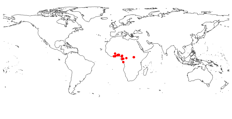
African pied hornbill

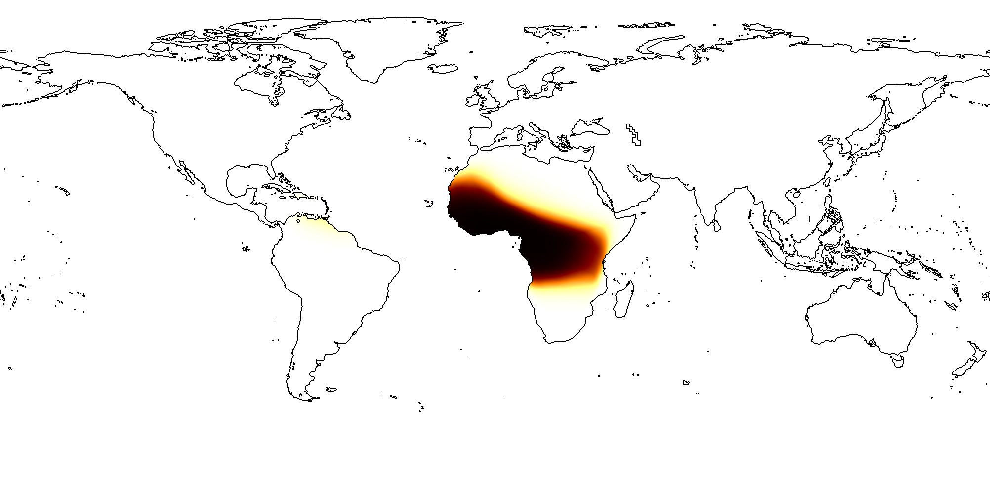
$wrap$

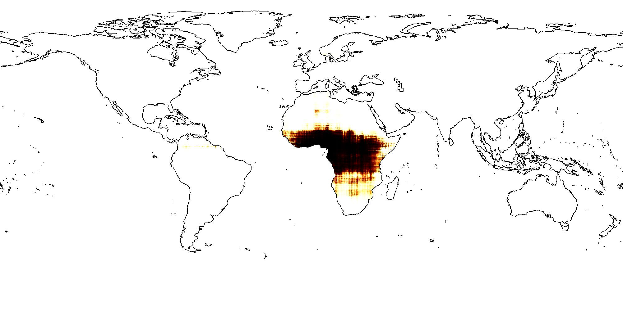
$grid$

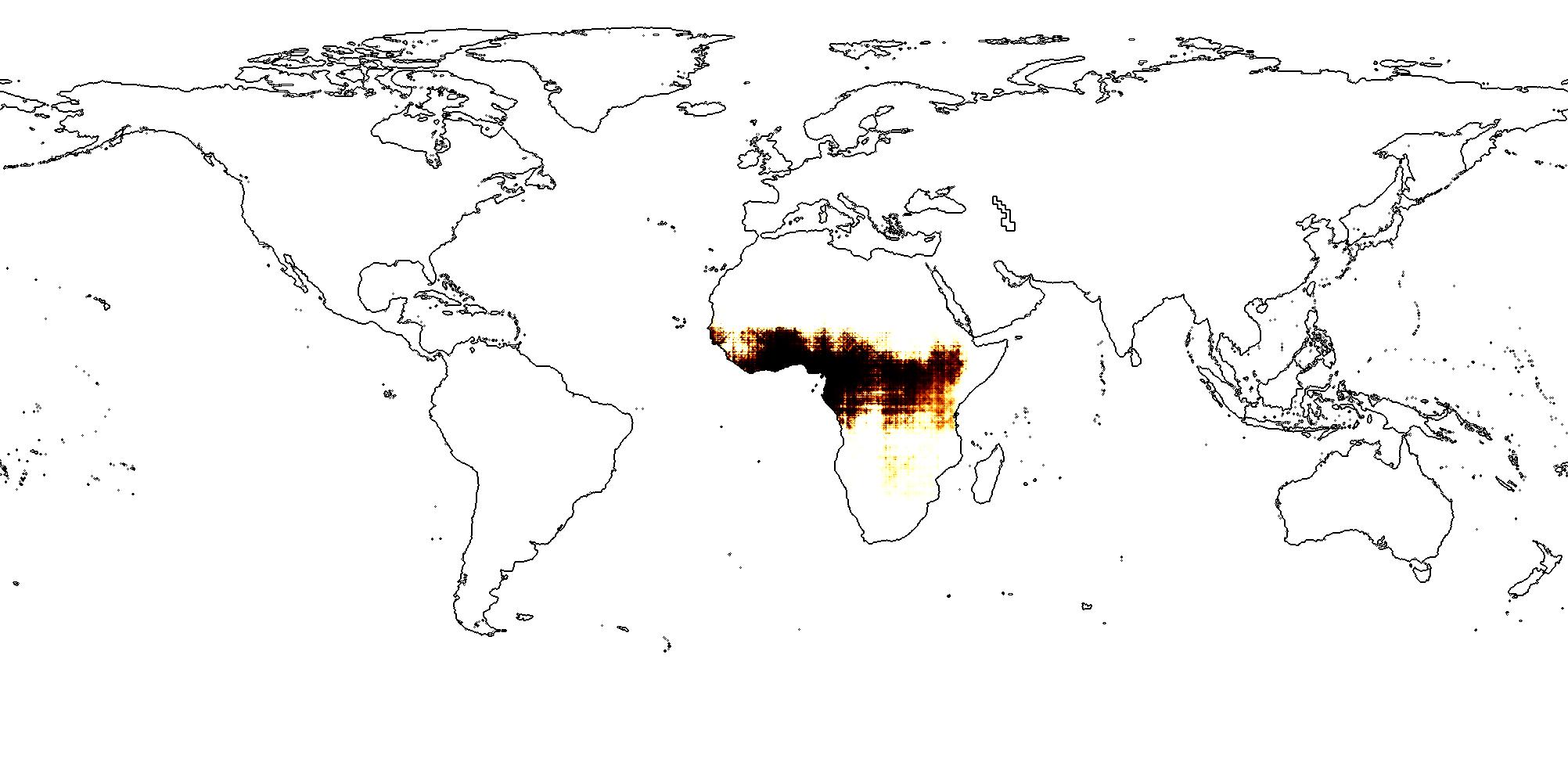
$sphereC+$

Image

White-browed wagtail

$wrap$

$grid$

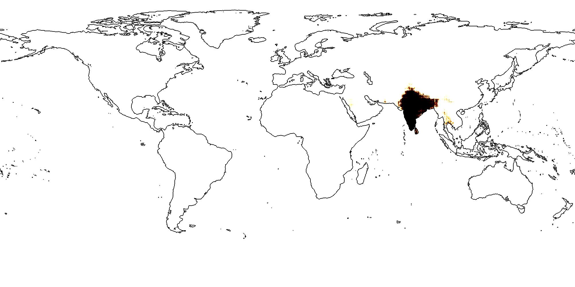
$sphereC+$

Image

Arctic Fox

$wrap$

$grid$

$sphereC+$

Image

Bat-Eared Fox

$wrap$

$grid$

$sphereC+$

Image

Red-striped leafwing

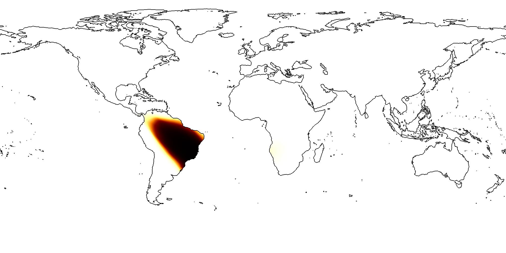
$wrap$

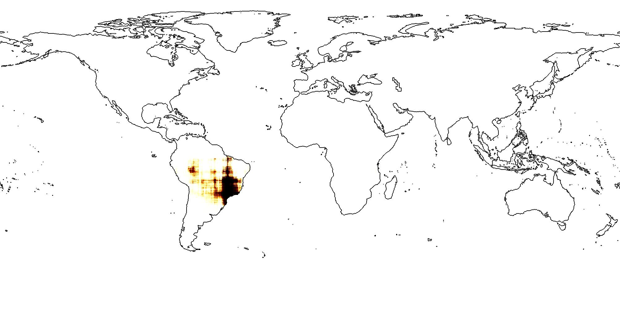
$grid$

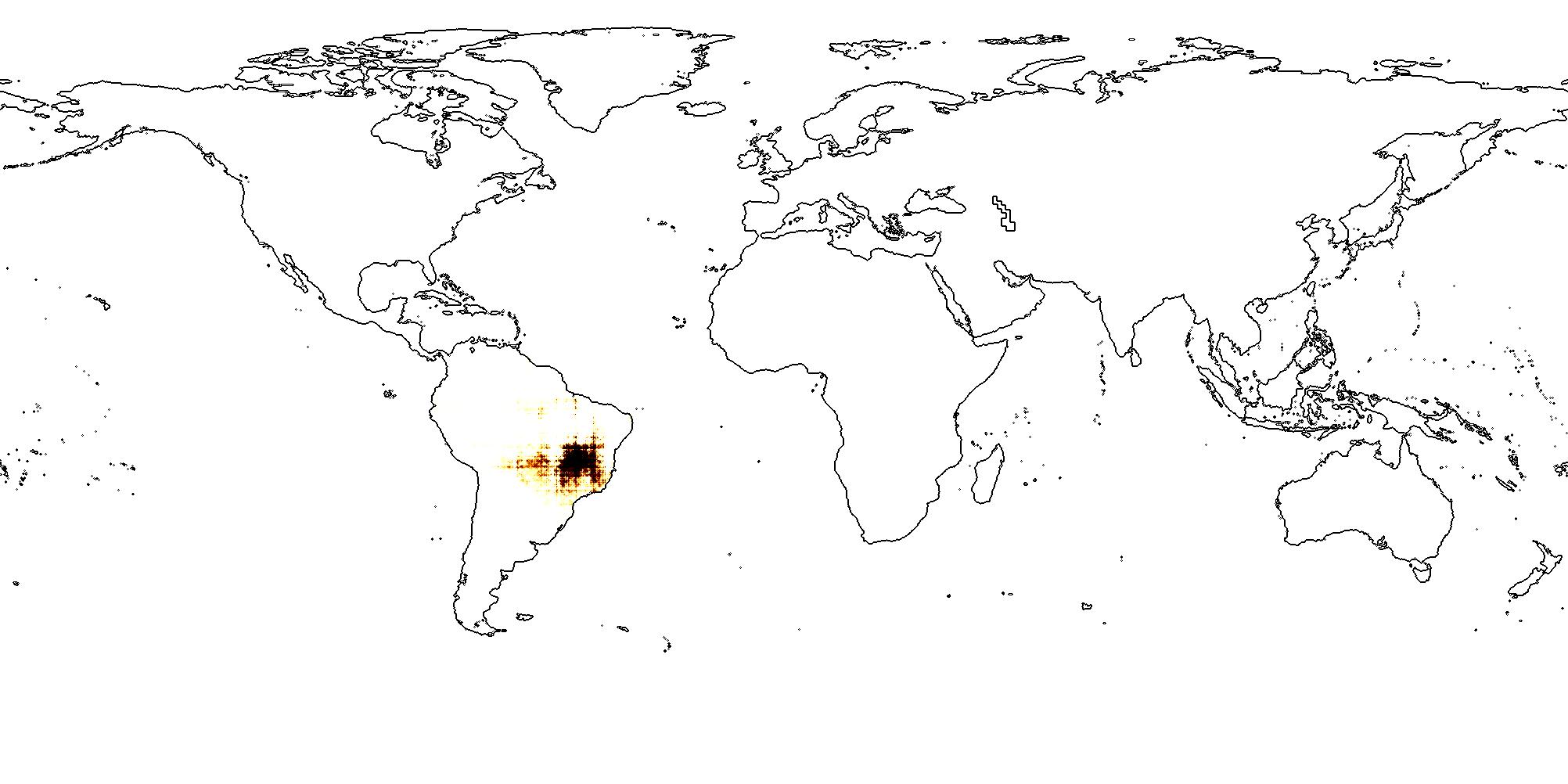
$sphereC+$

Image

False Tiger Moth

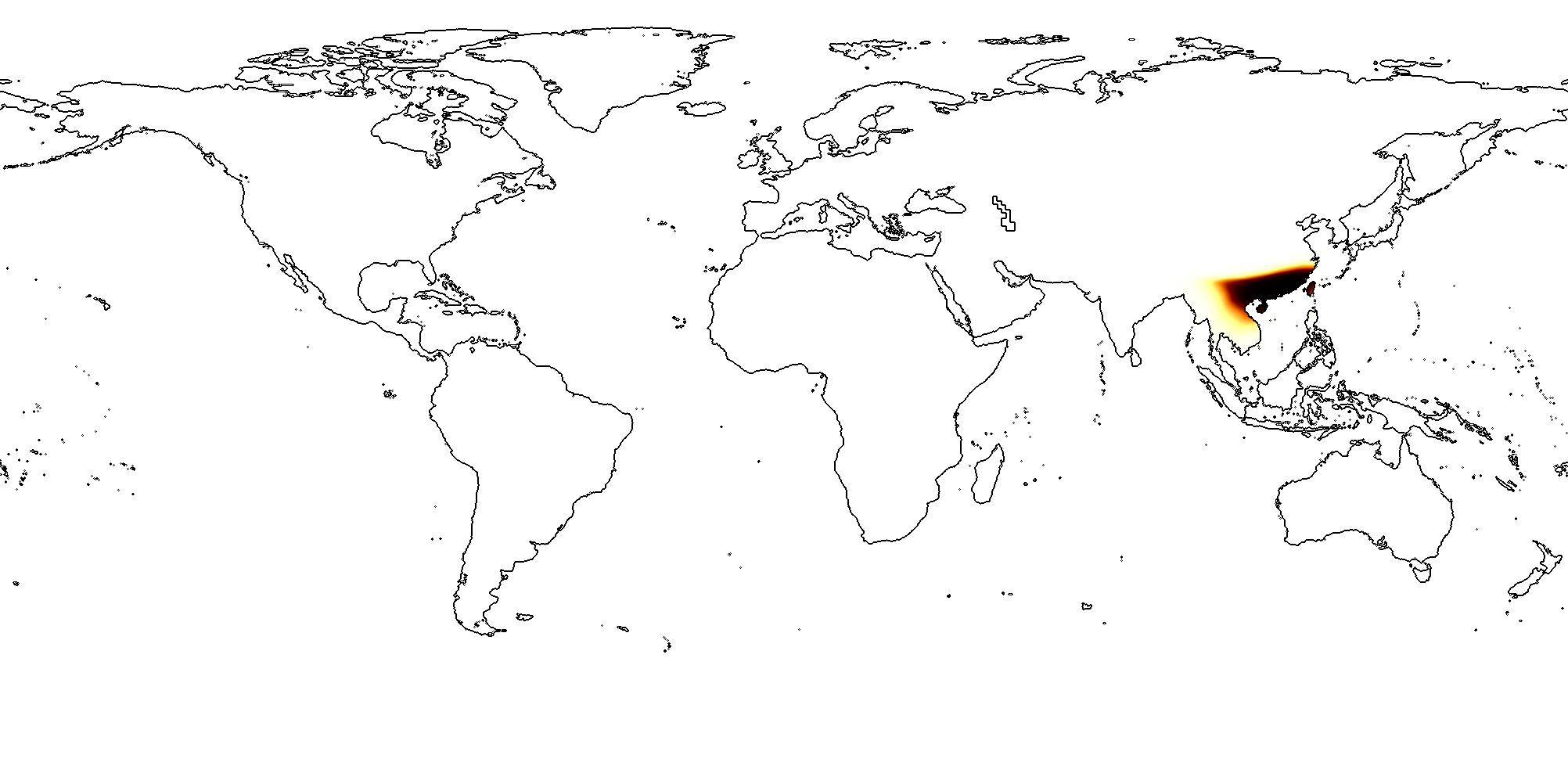
$wrap$

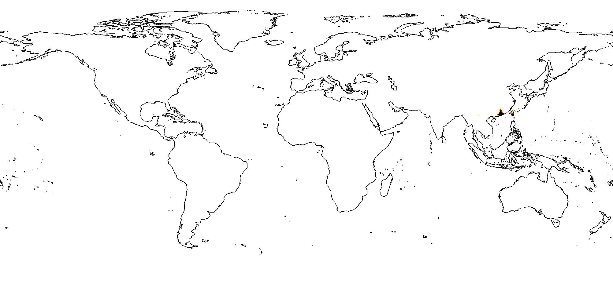
$grid$

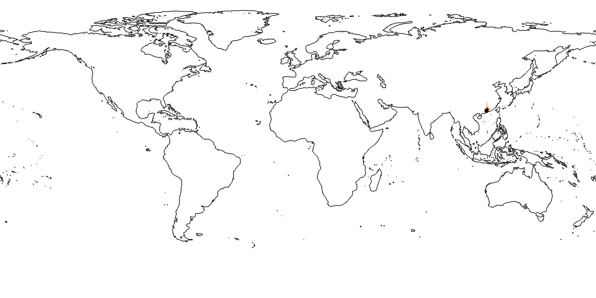
$sphereC+$

Figure 13: Comparison of the predicted spatial distributions of example species in the iNat2018 dataset from different location encoders. Each row indicates one specific species. We show one marine polychaete worm species, two bird species, two fox species, and two butterfly species. The first and second figure of each row show an example figure as well as the data points of this species from iNat2018 training data.

Image

Factory or powerplant

$wrap$

$grid$

$dfs$

Image

Multi-unit residential

$wrap$

$grid$

$dfs$

Image

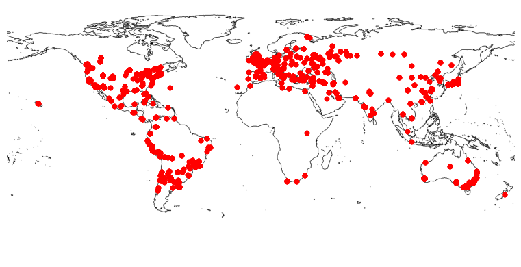
Park

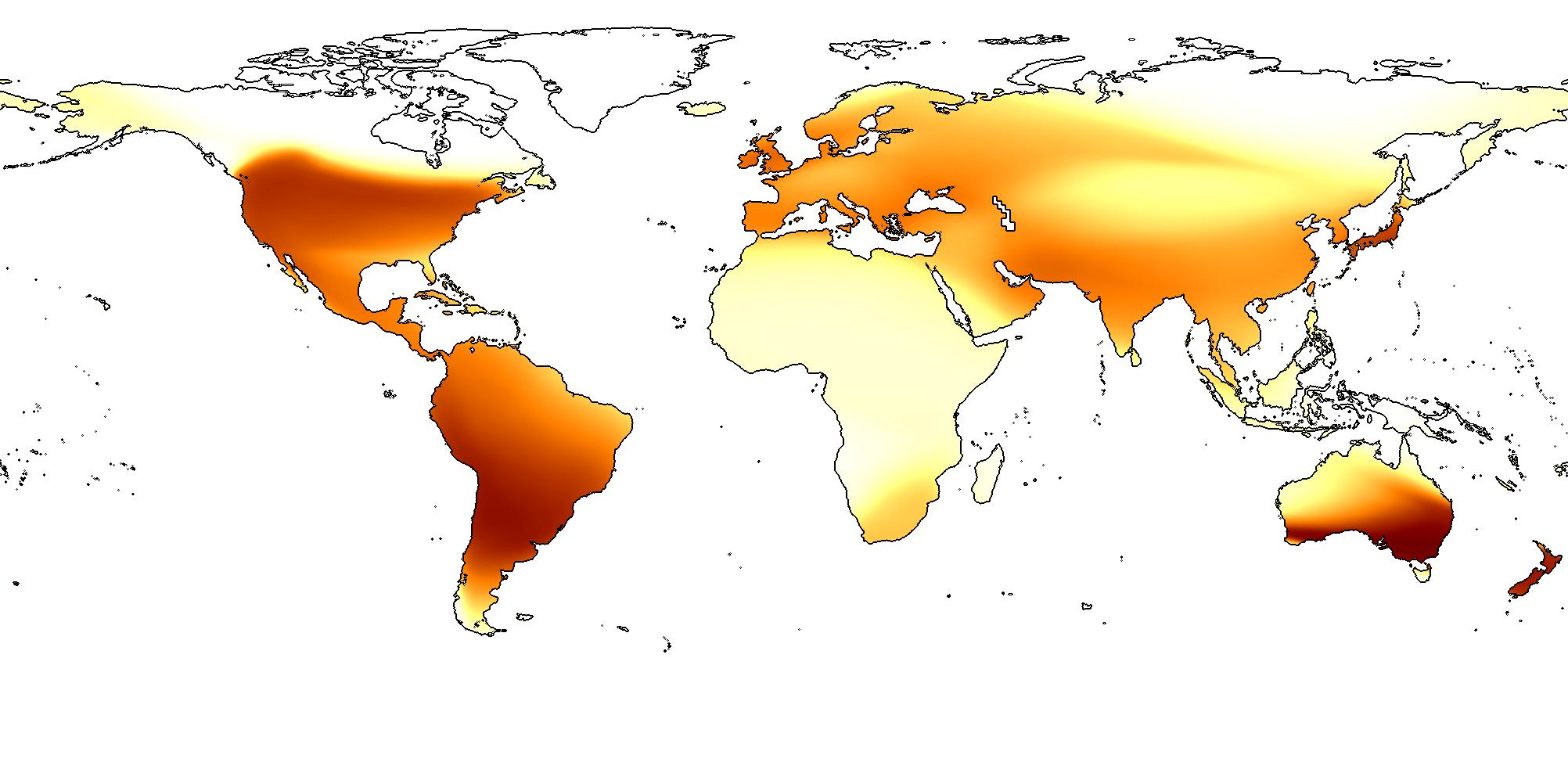
$wrap$

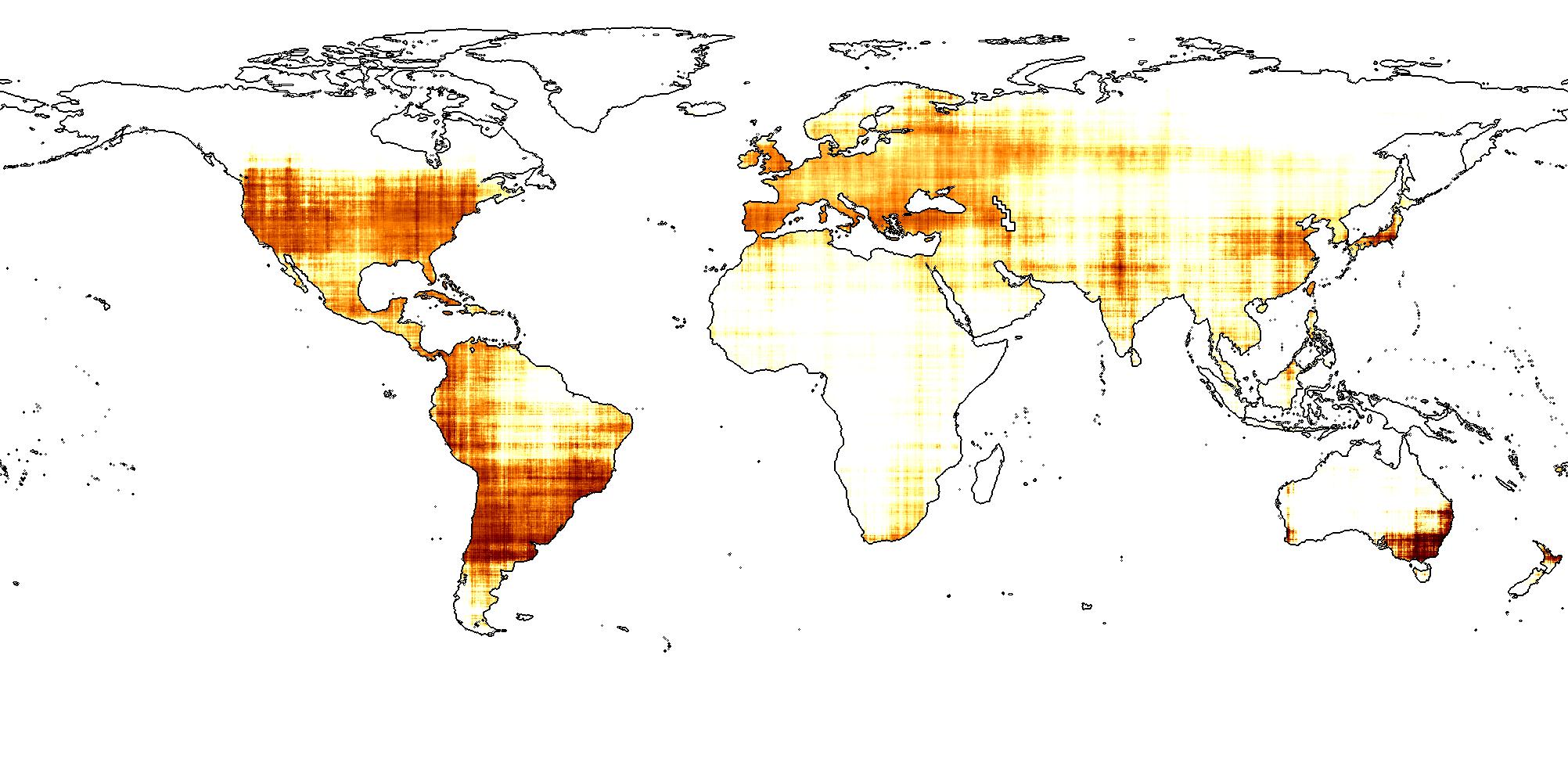
$grid$

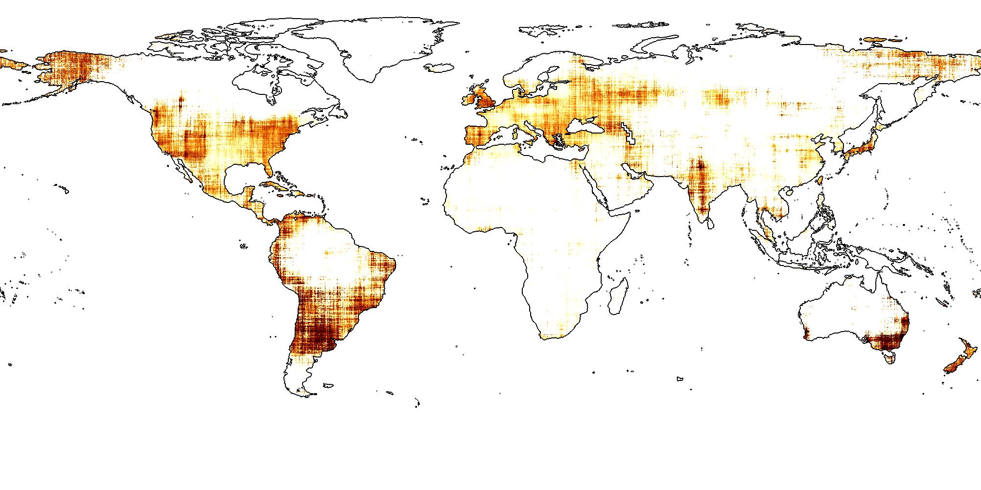
$dfs$

Image

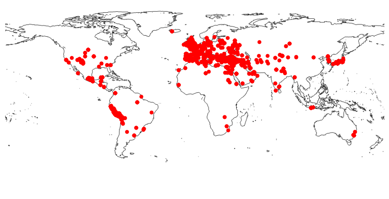
Archaeological site

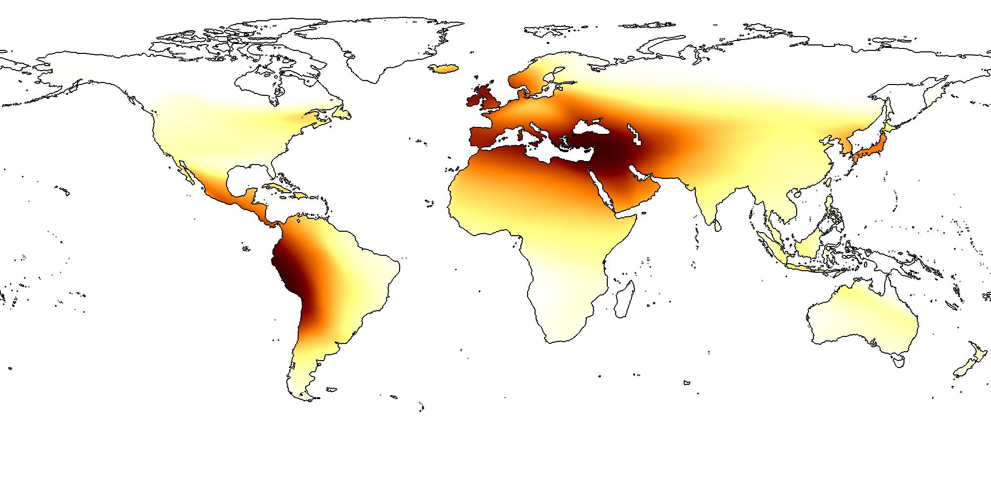
$wrap$

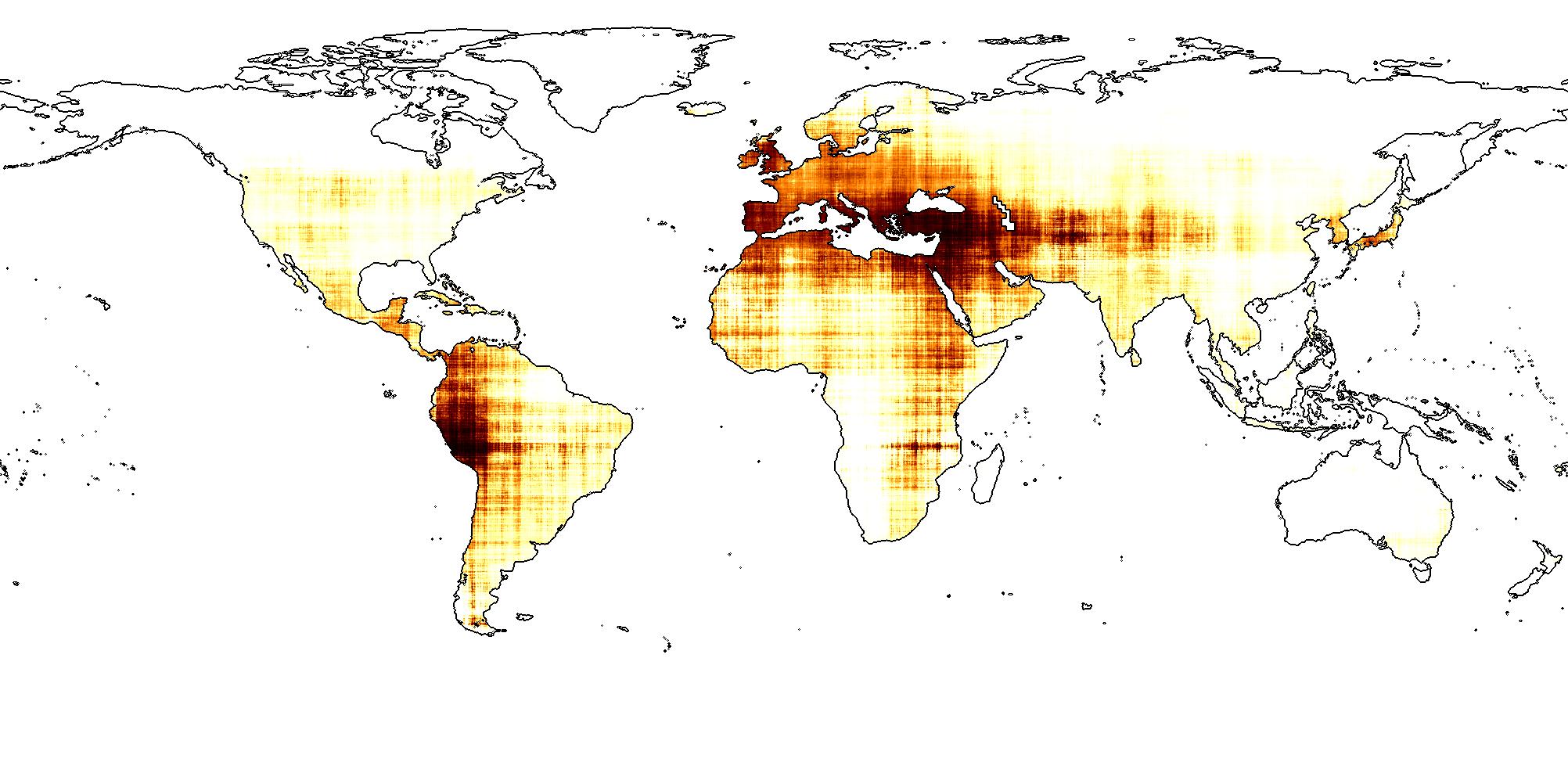
$grid$

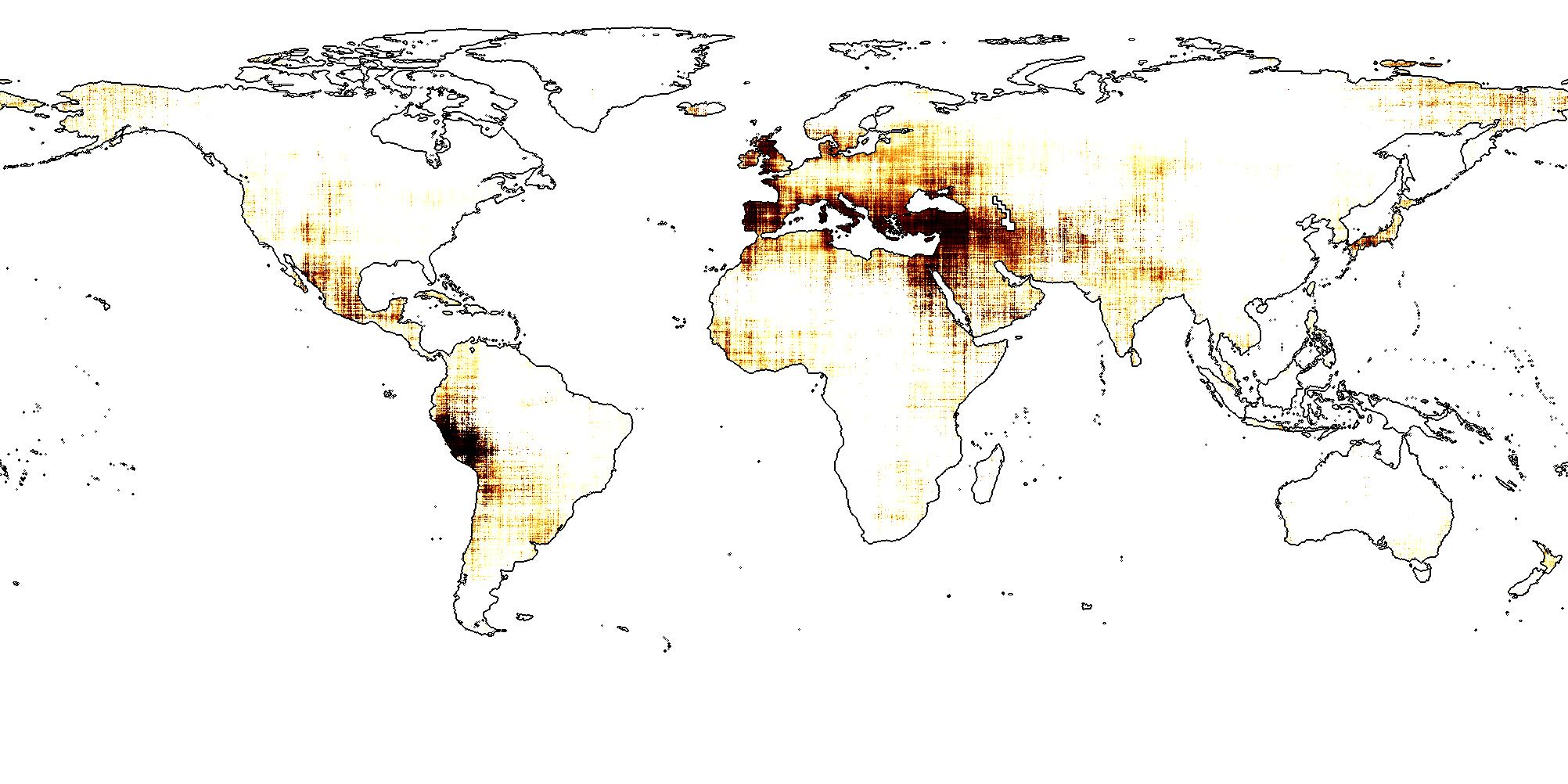
$dfs$

Figure 14: Comparison of the predicted spatial distributions of example land use types in the fMoW dataset from different location encoders. Each row indicates one specific land use type. The first and second figure of each row show an example figure as well as the data points of this land use types from the fMoW training data. As shown in Figure (a) and (f), although factories or powerplants and multi-unit residential type look very similar from overhead satellite imageries, they have very distinct spatial distribution (Figure (b) and (g)). Similarly, parks and archaeological sites look similar from satellites imageries (Figure (k) and (p)) which are usually covered by vegetation. However, they have very distinct spatial distribution (Figure (l) and (q)). We compare the predicted spatial distribution of each land use type from three different location encoders: $wrap$, $grid$, and $dfs$.

9.6.1 Predicted Species Distribution for iNat2018

From Figure 13, we can see that $wrap$ (Mac Aodha et al., 2019) produces rather over-generalized species distributions due to the fact that it is a single-scale location encoder. $sphereC+$ (our model) produces a more compact and fine-grained distribution in each geographic region, especially in the polar region and in data-sparse areas such as Africa and Asia. The distributions produced by $grid$ (Mai et al., 2020b) are between these two. However, $grid$ has limited spatial distribution modeling ability in the polar area (e.g., Figure 13 and 13) as well as data-sparse regions.

For example, in the white-browed wagtail example, $wrap$ produces an over-generalized spatial distribution which covers India, East Saudi Arabia, and the Southwest of China (See Figure 13). However, according to the training sample locations (Figure 13), white-browed wagtails only occur in India. $grid$ is better than $wrap$ but still produces a distribution covering the Southwest of China. $sphereC+$ produces the best compact distribution estimation. Similarly, for the red-striped leafwing, the sample locations are clustered in a small region in West Africa while $wrap$ produces an over-generalized distribution (see Figure 13). $grid$ produces a better distribution estimation (see Figure 13) but it still has a over-generalized issue. Our $sphereC+$ produces the best estimation among these three models – a compact distribution estimation covering the exact West Africa region (See Figure 13).

9.6.2 Predicted Land Use Distribution for fMoW

Similar visualizations are made for some example land use types in the fMoW dataset, i.e., Figure 14. Factories/powerplants (Figure 14) might look similar to multi-unit residential buildings (Figure 14) from overhead satellite imageries. But they have very different geographic distributions (Figure 14 and 14). A similarly situation can be seen for parks (Figure 14 and 14) and archaeological sites (Figure 14 and 14).

The estimated spatial distributions of these four land use types from three location encoders, i.e., $wrap$, $grid$, and $dfs$ are visualized. Just like what we see from Figure 13, similar observations can be made. $wrap$ usually produces over-generalized distributions. $dfs$ generates more compact and accurate distributions while $grid$ is between these two. We also find out that $grid$ will generate some grid-like patterns due to the use of sinusoidal functions. $dfs$ suffers less from it and produces more accurate distributions.

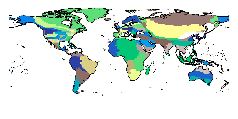
$wrap$

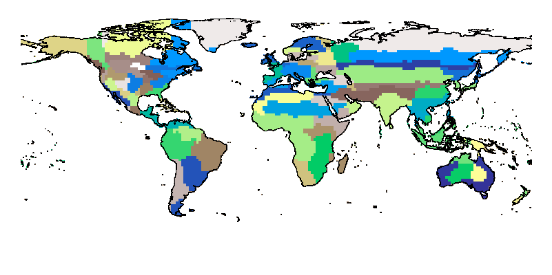
$grid$ $(r_{min}=10^{-2})$

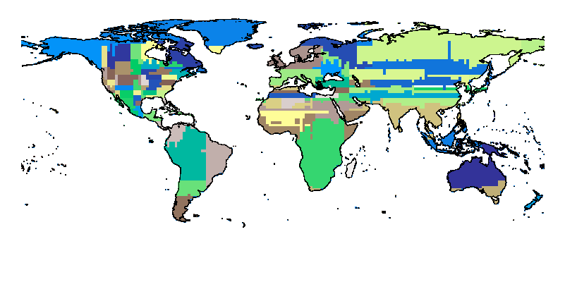
$grid$ $(r_{min}=10^{-6})$

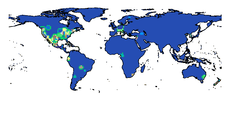
$rbf$ $(\sigma=1,m=200)$

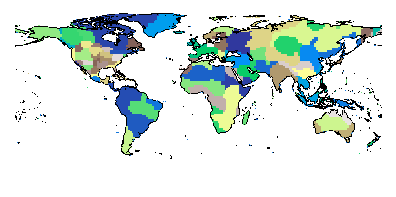
$theory$ $(r_{min}=10^{-2})$

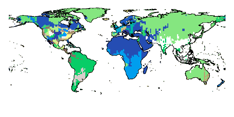
$theory$ $(r_{min}=10^{-6})$

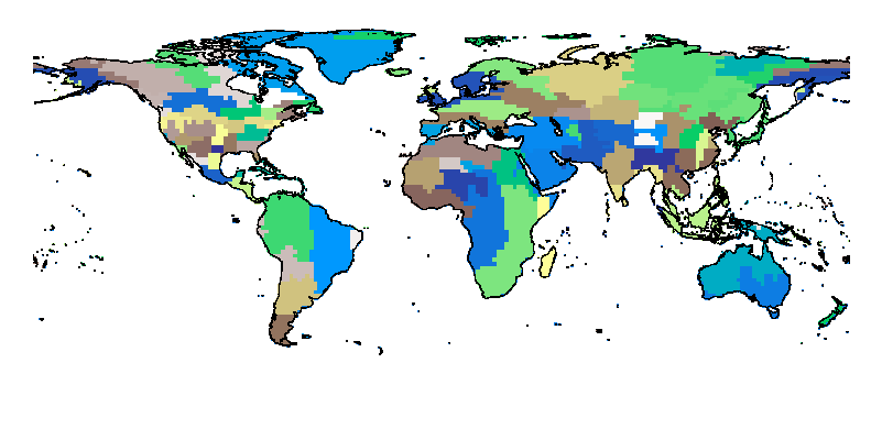
$NeRF$ $(S=32)$

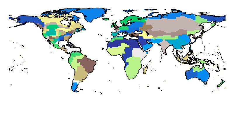
$sphereM$ $(r_{min}=10^{-1})$

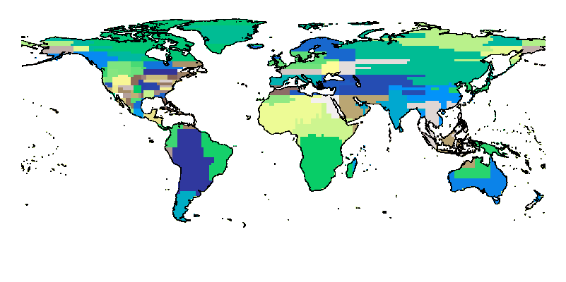
$sphereM$ $(r_{min}=10^{-2})$

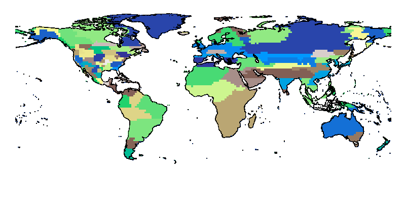
$sphereC$ $(r_{min}=10^{-2})$

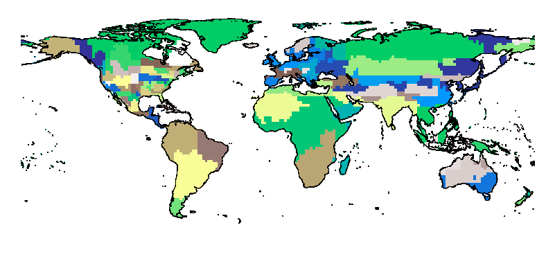
$sphereC+$ $(r_{min}=10^{-2})$

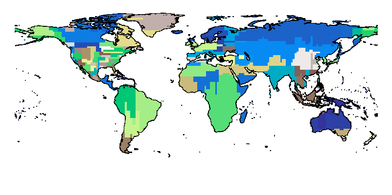
$sphereM+$ $(r_{min}=10^{-2})$

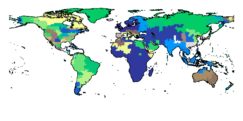
$dfs$ $(r_{min}=10^{-2})$

Figure 15: Embedding clusterings of different location encoders trained on the iNat2017 dataset. (a) $wrap*$ with 4 hidden ReLU layers of 256 neurons; (d) $rbf$ with the best kernel size $\sigma=1$ and number of anchor points $m=200$; (b)(c)(e)(f) are Space2Vec models (Mai et al., 2020b) with different min scale $r_{min}=\{10^{-6},10^{-2}\}$.^a (g) is $NeRF$ with $r_{min}=32$, and 1 hidden ReLU layer of 512 neurons. (h)-(m) are different Sphere2Vec models.^b

^a They share the same best hyperparameters: $S=64$, $r_{max}=1$, and 1 hidden ReLU layers of 512 neurons.
^bThey share the same best hyperparameters: $S=32$, $r_{max}=1$, and 1 hidden ReLU layers of 1024 neurons.

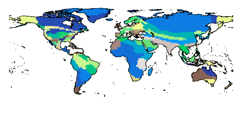
$wrap$

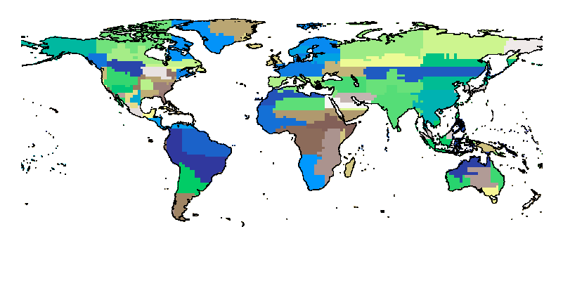
$grid$ $(r_{min}=10^{-3})$

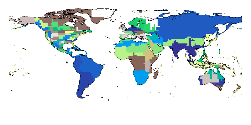
$grid$ $(r_{min}=10^{-6})$

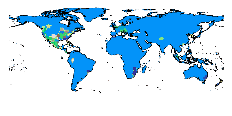
$rbf$ $(\sigma=1,m=200)$

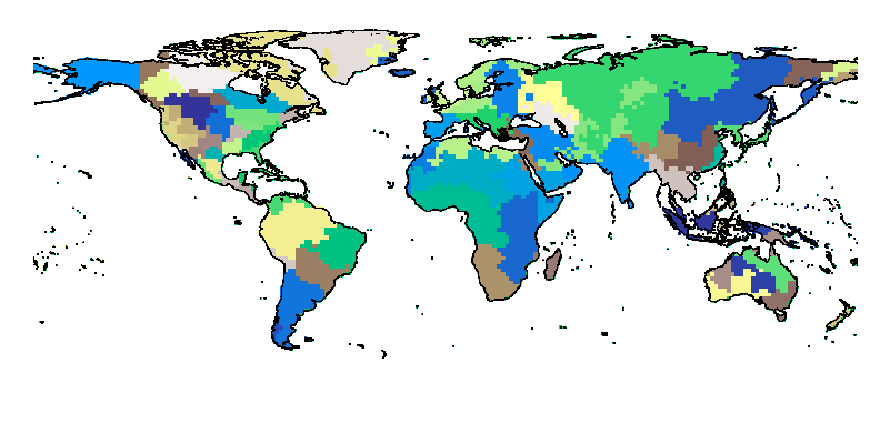
$theory$ $(r_{min}=10^{-3})$

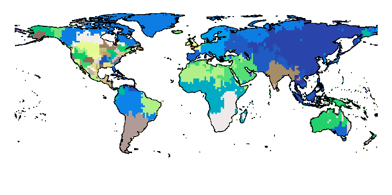
$theory$ $(r_{min}=10^{-6})$

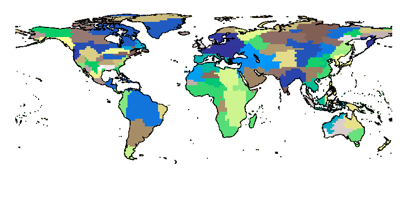
NeRF$NeRF$ $(S=32)$

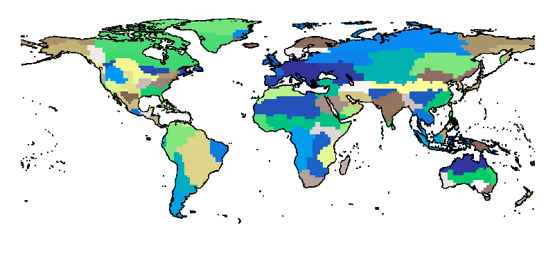
$sphereM$ $(r_{min}=10^{-1})$

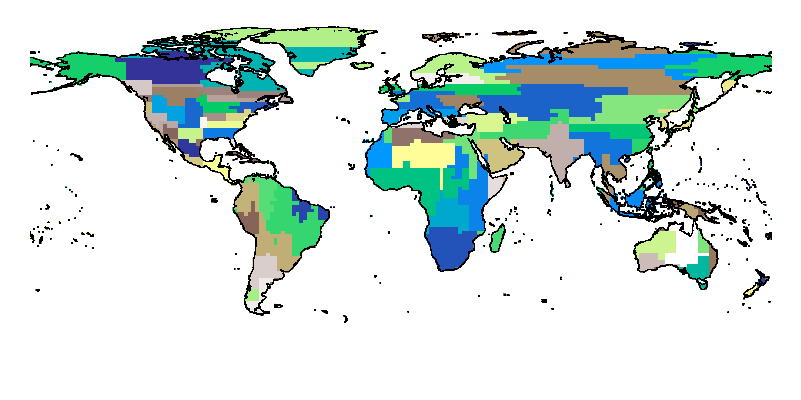
$sphereM$ $(r_{min}=10^{-3})$

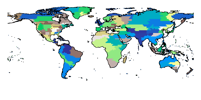
$sphereC$ $(r_{min}=10^{-3})$

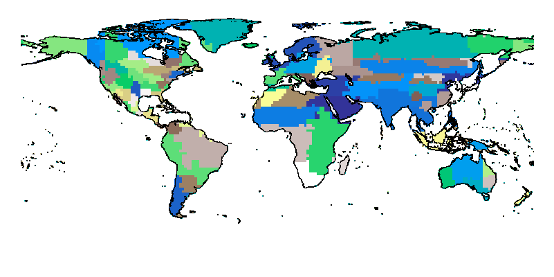
$sphereC+$ $(r_{min}=10^{-3})$

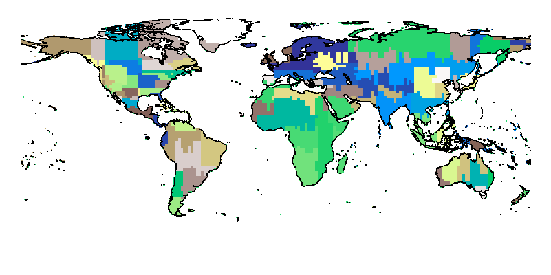
$sphereM+$ $(r_{min}=10^{-3})$

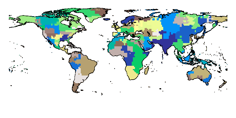
$dfs$ $(r_{min}=10^{-3})$

Figure 16: Embedding clusterings of different location encoders trained on the iNat2018 dataset. (a) $wrap$ with 4 hidden ReLU layers of 256 neurons; (d) $rbf$ with the best kernel size $\sigma=1$ and number of anchor points $m=200$; (b)(c)(e)(f) are Space2Vec models (Mai et al., 2020b) with different min scale $r_{min}=\{10^{-6},10^{-3}\}$.^a (g) is $NeRF$ with $r_{min}=32$, and 1 hidden ReLU layer of 512 neurons. (h)-(m) are Sphere2Vec models with different min scale $r_{min}$.^b

^a They share the same best hyperparameters: $S=64$, $r_{max}=1$, and 1 hidden ReLU layer of 512 neurons.
^bThey share the same best hyperparameters: $S=32$, $r_{max}=1$, and 1 hidden ReLU layers of 1024 neurons.

9.7 Location Embedding Clustering

To show how the trained location encoders learn the image label distributions, we divide the globe into small latitude-longitude cells and use a location encoder (e.g., Sphere2Vec or other baseline location encoders) trained on the iNat2017 or iNat2018 dataset to produce a location embedding for the center of each cell. Then we do agglomerative clustering on all these embeddings to produce a clustering map. Figure 15 and 16 show the clustering results for different models with different hyperparameters on the iNat2017 and iNat2018 datasets.

From Figure 15, we can see that:

1. In all these clustering maps, nearby locations are clustered together which indicates their location embeddings are similar to each other. This confirms that the learned location encoder can preserve distance information.

2. In the $rbf$ clustering map shown in Figure 15, except North America, almost all the other regions are in the same cluster. This is because compared with North America, all other regions have fewer training samples. This indicates that $rbf$ can not generate a reliable spatial distribution estimation in data-sparse regions.

3. The clustering maps of $grid$ (Figure 15 and 15) show horizontal strip-like clusters. More specifically, in Figure 15, the boundaries of many clusters are parallel to the longitude and latitude lines. We hypothesize that these kinds of artifacts are created because $grid$ measures the latitude and longitude differences separately (see Theorem 3) which cannot measure the spherical distance correctly.

4. $wrap$ (Figure 15), $sphereM$ (Figure 15, $sphereC$ (Figure 15), $sphereC+$ (Figure 15), $sphereM+$ (Figure 15), and $dfs$ (Figure 15) show reasonable geographic clustering maps. Each cluster has rather naturally looked curvilinear boundaries rather than linear boundaries. We think this reflects the true mixture of different species distributions. However, as we showed in Section 9.6, the single-scale $wrap$ produces over-generalized distribution while Sphere2Vec can produce more compact distribution estimation.

Similar conclusions can be drawn from Figure 16. We believe those figures visually demonstrate the superiority of Sphere2Vec.

10 Conclusion

In this work, we propose a general-purpose multi-scale spherical location encoder - Sphere2Vec which can encode any location on the spherical surface into a high dimensional vector which is learning-friendly for downstream neuron network models. We provide theoretical proof that Sphere2Vec is able to preserve the spherical surface distance between points. As a comparison, we also prove that the 2D location encoders such as $grid$ (Gao et al., 2019; Mai et al., 2020b) model the latitude and longitude difference of two points separately. And NeRF-style 3D location encoders (Mildenhall et al., 2020; Schwarz et al., 2020; Niemeyer and Geiger, 2021) model the axis-wise differences between two points in 3D Euclidean space separately. Both of them cannot model the true spherical distance. To verify the superiority of Sphere2Vec in a controlled setting, we generate 20 synthetic datasets and evaluate Sphere2Vec and all baselines on them. Results show that Sphere2Vec can outperform all baselines on all 20 sythetic datasets and the error rate reduction can go up to 30.8%. The results indicate that when the underlying dataset has a larger data bias towards the polar area, we expect a bigger performance improvement of Sphere2Vec. We further conduct experiments on three geo-aware image classification tasks with 7 large-scale real-world datasets. Results shows that Sphere2Vec can outperform the state-of-the-art 2D location encoders on all 7 datasets. Further analysis shows that Sphere2Vec is especially excel at polar regions as well data-sparse areas.

Encoding point-features on a spherical surface is a fundamental problem, especially in geoinformatics, geography, meteorology, oceanography, geoscience, and environmental science. Our proposed Sphere2Vec is a general-purpose spherical-distance-reserving encoding which realizes our idea of directly calculating on the round planet. It can be utilized in a wide range of geospatial prediction tasks. In this work, we only conduct experiments on geo-aware image classification and spatial distribution estimation. Except for the tasks we discussed above, the potential applications include areas like public health, epidemiology, agriculture, economy, ecology, and environmental engineering, and researches like large-scale human mobility and trajectory prediction (Xu et al., 2018), geographic question answering (Mai et al., 2020a), global biodiversity hotspot prediction (Myers et al., 2000; Di Marco et al., 2019; Ceballos et al., 2020), weather forecasting and climate change (Dupont et al., 2021; Ham et al., 2019), global pandemic study and its relation to air pollution (Wu et al., 2020), and so on. In general, we expect our proposed Sphere2Vec will benefit various AI for social goods applications which involve predictive modeling at global scales. Moreover, Sphere2Vec can also contribute to the idea of developing a foundation model for geospatial artificial intelligence (Mai et al., 2022c, 2023a) in general.

Declaration of Competing Interest

The authors declare that they have no known competing financial interests or personal relationships that could have appeared to influence the work reported in this paper.

Appendix A Theoretical Proofs of Each Theorem

A.1 Proof of Theorem 1

Proof.

Given two points $\boldsymbol{\mathbf{x}}_{1}=(\lambda_{1},\phi_{1}),\boldsymbol{\mathbf{x}}_{2}=(\lambda_{2},\phi_{2})$ on the same sphere $\mathbb{S}^{2}$ with radius $R$, we have $PE^{sphereC}_{1}(\boldsymbol{\mathbf{x}}_{i})=[\sin(\phi_{i}),\cos(\phi_{i})\cos(\lambda_{i}),\cos(\phi_{i})\sin(\lambda_{i})]$ for $i=1,2$, the inner product

$$\begin{split}&\langle PE^{sphereC}_{1}(\boldsymbol{\mathbf{x}}_{1}),PE^{sphereC}_{1}(\boldsymbol{\mathbf{x}}_{2})\rangle\\ &=\sin(\phi_{1})\sin(\phi_{2})+\cos(\phi_{1})\cos(\lambda_{1})\cos(\phi_{2})\cos(\lambda_{2})\\ &+\cos(\phi_{1})\sin(\lambda_{1})\cos(\phi_{2})\sin(\lambda_{2})\\ &=\sin(\phi_{1})\sin(\phi_{2})+\cos(\phi_{1})\cos(\phi_{2})\cos(\lambda_{1}-\lambda_{2})\\ &=\cos(\Delta\delta)=\cos(\Delta D/R),\end{split}$$ (28)

where $\Delta\delta$ is the central angle between $\boldsymbol{\mathbf{x}}_{1}$and $\boldsymbol{\mathbf{x}}_{2}$, and the spherical law of cosines is applied to derive the second last equality. So,

$$\begin{split}&\|PE^{sphereC}_{1}(\boldsymbol{\mathbf{x}}_{1})-PE^{sphereC}_{1}(\boldsymbol{\mathbf{x}}_{2})\|^{2}\\ =&\langle PE^{sphereC}_{1}(\boldsymbol{\mathbf{x}}_{1})-PE^{sphereC}_{1}(\boldsymbol{\mathbf{x}}_{2}),\\ &PE^{sphereC}_{1}(\boldsymbol{\mathbf{x}}_{1})-PE^{sphereC}_{1}(\boldsymbol{\mathbf{x}}_{2})\rangle\\ =&2-2\cos(\Delta D/R)\\ =&4\sin^{2}(\Delta D/2R).\end{split}$$ (29)

So $\|PE^{sphereC}_{1}(\boldsymbol{\mathbf{x}}_{1})-PE^{sphereC}_{1}(\boldsymbol{\mathbf{x}}_{2})\|=2\sin(\Delta D/2R)$ since $\Delta D/2R\in[0,\frac{\pi}{2}]$. By Taylor expansion, $\|PE^{sphereC}_{1}(\boldsymbol{\mathbf{x}}_{1})-PE^{sphereC}_{1}(\boldsymbol{\mathbf{x}}_{2})\|\approx\Delta D/R$ when $\Delta D$ is small w.r.t. $R$. ∎

A.2 Proof of Theorem 2

Proof.

$\forall*\in\{sphereC,sphereC+,sphereM,sphereM+\}$, $PE^{*}_{S}(\boldsymbol{\mathbf{x}}_{1})=PE^{*}_{S}(\boldsymbol{\mathbf{x}}_{2})$ implies

$$\sin(\phi_{1})=\sin(\phi_{2}),$$ (30)

$$\cos(\phi_{1})\sin(\lambda_{1})=\cos(\phi_{2})\sin(\lambda_{2}),$$ (31)

$$\cos(\phi_{1})\cos(\lambda_{1})=\cos(\phi_{2})\cos(\lambda_{2}),$$ (32)

from $s=0$ terms. Since $\sin(\phi)$ monotonically increases when $\phi\in[-{\pi}/{2},{\pi}/{2}]$, given Equation 30 we have $\phi_{1}=\phi_{2}$. If $\phi_{1}=\phi_{2}=\pi/2$, then both points are at North Pole, $\lambda_{1}=\lambda_{2}$ equal to whatever longitude defined at North Pole. If $\phi_{1}=\phi_{2}=-\pi/2$, it is similar case at South Pole. When $\phi_{1}=\phi_{2}\in(-\frac{\pi}{2},\frac{\pi}{2})$, $\cos(\phi_{1})=\cos(\phi_{2})\neq 0$. Then from Equation 31 and 32, we have

$$\sin{\lambda_{1}}=\sin(\lambda_{2}),\cos(\lambda_{1})=\cos(\lambda_{2}),$$ (33)

which shows that $\lambda_{1}=\lambda_{2}$. In summary, $\boldsymbol{\mathbf{x}}_{1}=\boldsymbol{\mathbf{x}}_{2}$, so $PE^{*}_{S}$ is injective.
If $*=dfs$, $PE^{*}_{S}(\boldsymbol{\mathbf{x}}_{1})=PE^{*}_{S}(\boldsymbol{\mathbf{x}}_{2})$ implies $\sin(\phi_{1})=\sin(\phi_{2})$, $\cos(\phi_{1})=\cos(\phi_{2})$, $\sin(\lambda_{1})=\sin(\lambda_{2})$, and $\cos(\lambda_{1})=\cos(\lambda_{2})$, which proves $\boldsymbol{\mathbf{x}}_{1}=\boldsymbol{\mathbf{x}}_{2}$ and $PE^{*}_{S}$ is injective directly. ∎

A.3 Proof of Theorem 4

Proof.

According to the definition of $NeRF$ encoder (18),

$$\begin{split}&\|PE^{NeRF}_{S}(\boldsymbol{\mathbf{x}}_{1})-PE^{NeRF}_{S}(\boldsymbol{\mathbf{x}}_{2})\|^{2}\\ &=\sum_{s=0}^{S-1}\sum_{p\in\{z,x,y\}}\Big{(}(\sin(2^{s}\pi p_{1})-\sin(2^{s}\pi p_{2}))^{2}\\ &\qquad+(\cos(2^{s}\pi p_{1})-\cos(2^{s}\pi p_{2}))^{2}\Big{)}\\ &=\sum_{s=0}^{S-1}\sum_{p\in\{z,x,y\}}\Big{(}\sin^{2}(2^{s}\pi p_{1})+\sin^{2}(2^{s}\pi p_{2})\\ &\qquad-2\sin(2^{s}\pi p_{1})\sin(2^{s}\pi p_{2})\\ &\qquad+\cos^{2}(2^{s}\pi p_{1})+\cos^{2}(2^{s}\pi p_{2})\\ &\qquad-2\cos(2^{s}\pi p_{1})\cos(2^{s}\pi p_{2})\Big{)}\\ &=\sum_{s=0}^{S-1}\sum_{p\in\{z,x,y\}}\Big{(}2-2(\sin(2^{s}\pi p_{1})\sin(2^{s}\pi p_{2})\\ &\qquad+\cos(2^{s}\pi p_{1})\cos(2^{s}\pi p_{2}))\Big{)}\\ &=\sum_{s=0}^{S-1}\sum_{p\in\{z,x,y\}}\Big{(}2-2\cos(2^{s}\pi(p_{1}-p_{2}))\Big{)}\\ &=\sum_{s=0}^{S-1}\sum_{p\in\{z,x,y\}}4\sin^{2}(2^{s-1}\pi(p_{1}-p_{2}))\\ &=\sum_{s=0}^{S-1}\Big{(}4\sin^{2}(2^{s-1}\pi\Delta\boldsymbol{\mathbf{x}}_{z})+4\sin^{2}(2^{s-1}\pi\Delta\boldsymbol{\mathbf{x}}_{x})\\ &+4\sin^{2}(2^{s-1}\pi\Delta\boldsymbol{\mathbf{x}}_{y})\Big{)}\\ &=\sum_{s=0}^{S-1}4\|\boldsymbol{\mathbf{Y}}_{s}\|^{2},\end{split}$$ (34)

where $\boldsymbol{\mathbf{Y}}_{s}=[\sin(2^{s-1}\pi\Delta\boldsymbol{\mathbf{x}}_{z}),\sin(2^{s-1}\pi\Delta\boldsymbol{\mathbf{x}}_{x}),\sin(2^{s-1}\pi\Delta\boldsymbol{\mathbf{x}}_{y})]$. ∎

References

- Adams et al. (2015) Adams, B., McKenzie, G., Gahegan, M., 2015. Frankenplace: interactive thematic mapping for ad hoc exploratory search, in: Proceedings of the 24th international conference on world wide web, International World Wide Web Conferences Steering Committee. pp. 12–22.
- Anokhin et al. (2021a) Anokhin, I., Demochkin, K., Khakhulin, T., Sterkin, G., Lempitsky, V., Korzhenkov, D., 2021a. Image generators with conditionally-independent pixel synthesis, in: Proceedings of the IEEE/CVF Conference on Computer Vision and Pattern Recognition, pp. 14278–14287.
- Anokhin et al. (2021b) Anokhin, I., Demochkin, K., Khakhulin, T., Sterkin, G., Lempitsky, V., Korzhenkov, D., 2021b. Image generators with conditionally-independent pixel synthesis, in: Proceedings of the IEEE/CVF Conference on Computer Vision and Pattern Recognition, pp. 14278–14287.
- Ayush et al. (2020) Ayush, K., Uzkent, B., Meng, C., Tanmay, K., Burke, M., Lobell, D., Ermon, S., 2020. Geography-aware self-supervised learning. arXiv preprint arXiv:2011.09980 .
- Banino et al. (2018) Banino, A., Barry, C., Uria, B., Blundell, C., Lillicrap, T., Mirowski, P., Pritzel, A., Chadwick, M.J., Degris, T., Modayil, J., et al., 2018. Vector-based navigation using grid-like representations in artificial agents. Nature 557, 429.
- Barron et al. (2021) Barron, J.T., Mildenhall, B., Tancik, M., Hedman, P., Martin-Brualla, R., Srinivasan, P.P., 2021. Mip-nerf: A multiscale representation for anti-aliasing neural radiance fields, in: Proceedings of the IEEE/CVF International Conference on Computer Vision, pp. 5855–5864.
- Bartnik and Norton (2000) Bartnik, R., Norton, A., 2000. Numerical methods for the einstein equations in null quasi-spherical coordinates. SIAM Journal on Scientific Computing 22, 917–950.
- Basri et al. (2020) Basri, R., Galun, M., Geifman, A., Jacobs, D., Kasten, Y., Kritchman, S., 2020. Frequency bias in neural networks for input of non-uniform density, in: International Conference on Machine Learning, PMLR. pp. 685–694.
- Berg et al. (2014) Berg, T., Liu, J., Woo Lee, S., Alexander, M.L., Jacobs, D.W., Belhumeur, P.N., 2014. BirdSnap: Large-scale fine-grained visual categorization of birds, in: Proceedings of the IEEE Conference on Computer Vision and Pattern Recognition, pp. 2011–2018.
- Boyer (2012) Boyer, C.B., 2012. History of analytic geometry. Courier Corporation.
- Bronstein et al. (2017) Bronstein, M.M., Bruna, J., LeCun, Y., Szlam, A., Vandergheynst, P., 2017. Geometric deep learning: going beyond euclidean data. IEEE Signal Processing Magazine 34, 18–42.
- Caminade et al. (2014) Caminade, C., Kovats, S., Rocklov, J., Tompkins, A.M., Morse, A.P., Colón-González, F.J., Stenlund, H., Martens, P., Lloyd, S.J., 2014. Impact of climate change on global malaria distribution. Proceedings of the National Academy of Sciences 111, 3286–3291. URL: https://www.pnas.org/content/111/9/3286, doi:10.1073/pnas.1302089111, arXiv:https://www.pnas.org/content/111/9/3286.full.pdf.
- Ceballos et al. (2020) Ceballos, G., Ehrlich, P.R., Raven, P.H., 2020. Vertebrates on the brink as indicators of biological annihilation and the sixth mass extinction. Proceedings of the National Academy of Sciences URL: https://www.pnas.org/content/early/2020/05/27/1922686117, doi:10.1073/pnas.1922686117, arXiv:https://www.pnas.org/content/early/2020/05/27/1922686117.full.pdf.
- Chen et al. (2021) Chen, Y., Liu, S., Wang, X., 2021. Learning continuous image representation with local implicit image function, in: Proceedings of the IEEE/CVF conference on computer vision and pattern recognition, pp. 8628--8638.
- Chinazzi et al. (2020) Chinazzi, M., Davis, J.T., Ajelli, M., Gioannini, C., Litvinova, M., Merler, S., Pastore y Piontti, A., Mu, K., Rossi, L., Sun, K., Viboud, C., Xiong, X., Yu, H., Halloran, M.E., Longini, I.M., Vespignani, A., 2020. The effect of travel restrictions on the spread of the 2019 novel coronavirus (covid-19) outbreak. Science 368, 395--400. URL: https://science.sciencemag.org/content/368/6489/395, doi:10.1126/science.aba9757, arXiv:https://science.sciencemag.org/content/368/6489/395.full.pdf.
- Chrisman (2017) Chrisman, N.R., 2017. Calculating on a round planet. International Journal of Geographical Information Science 31, 637--657.
- Christie et al. (2018) Christie, G., Fendley, N., Wilson, J., Mukherjee, R., 2018. Functional map of the world, in: Proceedings of the IEEE Conference on Computer Vision and Pattern Recognition, pp. 6172--6180.
- Chu et al. (2019) Chu, G., Potetz, B., Wang, W., Howard, A., Song, Y., Brucher, F., Leung, T., Adam, H., 2019. Geo-aware networks for fine grained recognition, in: Proceedings of the IEEE International Conference on Computer Vision Workshops, pp. 0--0.
- Cohen et al. (2018) Cohen, T.S., Geiger, M., Köhler, J., Welling, M., 2018. Spherical CNNs, in: Proceedings of ICLR 2018.
- Coors et al. (2018) Coors, B., Paul Condurache, A., Geiger, A., 2018. SphereNet: Learning spherical representations for detection and classification in omnidirectional images, in: Proceedings of the European Conference on Computer Vision (ECCV), pp. 518--533.
- Cueva and Wei (2018) Cueva, C.J., Wei, X.X., 2018. Emergence of grid-like representations by training recurrent neural networks to perform spatial localization, in: International Conference on Learning Representations.
- Derksen and Izzo (2021) Derksen, D., Izzo, D., 2021. Shadow neural radiance fields for multi-view satellite photogrammetry, in: Proceedings of the IEEE/CVF Conference on Computer Vision and Pattern Recognition, pp. 1152--1161.
- Di Marco et al. (2019) Di Marco, M., Ferrier, S., Harwood, T.D., Hoskins, A.J., Watson, J.E.M., 2019. Wilderness areas halve the extinction risk of terrestrial biodiversity. Nature 573, 582--585. URL: https://doi.org/10.1038/s41586-019-1567-7, doi:10.1038/s41586-019-1567-7.
- (24) Dupont, E., Golinski, A., Alizadeh, M., Teh, Y.W., Doucet, A., . Coin: Compression with implicit neural representations, in: Neural Compression: From Information Theory to Applications--Workshop@ ICLR 2021.
- Dupont et al. (2021) Dupont, E., Teh, Y.W., Doucet, A., 2021. Generative models as distributions of functions. arXiv preprint arXiv:2102.04776 .
- Gao et al. (2019) Gao, R., Xie, J., Zhu, S.C., Wu, Y.N., 2019. Learning grid cells as vector representation of self-position coupled with matrix representation of self-motion, in: International Conference on Learning Representations.
- Gupta et al. (2021) Gupta, J., Molnar, C., Xie, Y., Knight, J., Shekhar, S., 2021. Spatial variability aware deep neural networks (svann): A general approach. ACM Transactions on Intelligent Systems and Technology (TIST) 12, 1--21.
- Ham et al. (2019) Ham, Y.G., Kim, J.H., Luo, J.J., 2019. Deep learning for multi-year enso forecasts. Nature 573, 568--572.
- Hansen and Cramer (2015) Hansen, G., Cramer, W., 2015. Global distribution of observed climate change impacts. Nature Climate Change 5, 182--185. URL: https://doi.org/10.1038/nclimate2529, doi:10.1038/nclimate2529.
- Harmel (2009) Harmel, A., 2009. Le nouveau système réglementaire lambert 93. Géomatique Expert 68, 26--30.
- He et al. (2021) He, Y., Wang, D., Lai, N., Zhang, W., Meng, C., Burke, M., Lobell, D., Ermon, S., 2021. Spatial-temporal super-resolution of satellite imagery via conditional pixel synthesis. Advances in Neural Information Processing Systems 34, 27903--27915.
- Helber et al. (2019) Helber, P., Bischke, B., Dengel, A., Borth, D., 2019. Eurosat: A novel dataset and deep learning benchmark for land use and land cover classification. IEEE Journal of Selected Topics in Applied Earth Observations and Remote Sensing 12, 2217--2226.
- Hu et al. (2019) Hu, Y., Gao, S., Lunga, D., Li, W., Newsam, S., Bhaduri, B., 2019. Geoai at acm sigspatial: progress, challenges, and future directions. Sigspatial Special 11, 5--15.
- Huang et al. (2023) Huang, W., Zhang, D., Mai, G., Guo, X., Cui, L., 2023. Learning urban region representations with pois and hierarchical graph infomax. ISPRS Journal of Photogrammetry and Remote Sensing 196, 134--145.
- Izbicki et al. (2019a) Izbicki, M., Papalexakis, E.E., Tsotras, V.J., 2019a. Exploiting the earth’s spherical geometry to geolocate images, in: Joint European Conference on Machine Learning and Knowledge Discovery in Databases, Springer. pp. 3--19.
- Izbicki et al. (2019b) Izbicki, M., Papalexakis, V., Tsotras, V., 2019b. Geolocating tweets in any language at any location, in: Proceedings of the 28th ACM International Conference on Information and Knowledge Management, pp. 89--98.
- Janowicz et al. (2020) Janowicz, K., Gao, S., McKenzie, G., Hu, Y., Bhaduri, B., 2020. GeoAI: Spatially explicit artificial intelligence techniques for geographic knowledge discovery and beyond.
- Janowicz et al. (2022) Janowicz, K., Hitzler, P., Li, W., Rehberger, D., Schildhauer, M., Zhu, R., Shimizu, C., Fisher, C.K., Cai, L., Mai, G., et al., 2022. Know, know where, knowwheregraph: A densely connected, cross-domain knowledge graph and geo-enrichment service stack for applications in environmental intelligence. AI Magazine 43, 30--39.
- Kejriwal and Szekely (2017) Kejriwal, M., Szekely, P., 2017. Neural embeddings for populated geonames locations, in: International Semantic Web Conference, Springer. pp. 139--146.
- Klocek et al. (2019) Klocek, S., Maziarka, L., Wolczyk, M., Tabor, J., Nowak, J., Smieja, M., 2019. Hypernetwork functional image representation, in: Tetko, I.V., Kurková, V., Karpov, P., Theis, F.J. (Eds.), Artificial Neural Networks and Machine Learning - ICANN 2019 - 28th International Conference on Artificial Neural Networks, Munich, Germany, September 17-19, 2019, Proceedings - Workshop and Special Sessions, Springer. pp. 496--510.
- Li et al. (2021) Li, W., Hsu, C.Y., Hu, M., 2021. Tobler’s first law in geoai: A spatially explicit deep learning model for terrain feature detection under weak supervision. Annals of the American Association of Geographers 111, 1887--1905.
- Liu and Biljecki (2022) Liu, P., Biljecki, F., 2022. A review of spatially-explicit geoai applications in urban geography. International Journal of Applied Earth Observation and Geoinformation 112, 102936.
- Mac Aodha et al. (2019) Mac Aodha, O., Cole, E., Perona, P., 2019. Presence-only geographical priors for fine-grained image classification, in: Proceedings of the IEEE International Conference on Computer Vision, pp. 9596--9606.
- Mai et al. (2022a) Mai, G., Hu, Y., Gao, S., Cai, L., Martins, B., Scholz, J., Gao, J., Janowicz, K., 2022a. Symbolic and subsymbolic geoai: Geospatial knowledge graphs and spatially explicit machine learning. Trans GIS 26, 3118--3124.
- Mai et al. (2023a) Mai, G., Huang, W., Sun, J., Song, S., Mishra, D., Liu, N., Gao, S., Liu, T., Cong, G., Hu, Y., et al., 2023a. On the opportunities and challenges of foundation models for geospatial artificial intelligence. arXiv preprint arXiv:2304.06798 .
- Mai et al. (2020a) Mai, G., Janowicz, K., Cai, L., Zhu, R., Regalia, B., Yan, B., Shi, M., Lao, N., 2020a. SE-KGE: A location-aware knowledge graph embedding model for geographic question answering and spatial semantic lifting. Transactions in GIS doi:10.1111/tgis.12629.
- Mai et al. (2022b) Mai, G., Janowicz, K., Hu, Y., Gao, S., Yan, B., Zhu, R., Cai, L., Lao, N., 2022b. A review of location encoding for geoai: methods and applications. International Journal of Geographical Information Science 36, 639--673.
- Mai et al. (2020b) Mai, G., Janowicz, K., Yan, B., Zhu, R., Cai, L., Lao, N., 2020b. Multi-scale representation learning for spatial feature distributions using grid cells, in: The Eighth International Conference on Learning Representations, openreview.
- Mai et al. (2023b) Mai, G., Jiang, C., Sun, W., Zhu, R., Xuan, Y., Cai, L., Janowicz, K., Ermon, S., Lao, N., 2023b. Towards general-purpose representation learning of polygonal geometries. GeoInformatica 27, 289--340.
- Mai et al. (2023c) Mai, G., Lao, N., He, Y., Song, J., Ermon, S., 2023c. Csp: Self-supervised contrastive spatial pre-training for geospatial-visual representations, in: International Conference on Machine Learning, PMLR.
- Mai et al. (2019) Mai, G., Yan, B., Janowicz, K., Zhu, R., 2019. Relaxing unanswerable geographic questions using a spatially explicit knowledge graph embedding model, in: AGILE: The 22nd Annual International Conference on Geographic Information Science, Springer. pp. 21--39.
- Mai et al. (2022c) Mai, G.M., Cundy, C., Choi, K., Hu, Y., Lao, N., Ermon, S., 2022c. Towards a foundation model for geospatial artificial intelligence, in: Proceedings of the 30th SIGSPATIAL international conference on advances in geographic information systems. doi:10.1145/3557915.3561043.
- Marí et al. (2022) Marí, R., Facciolo, G., Ehret, T., 2022. Sat-nerf: Learning multi-view satellite photogrammetry with transient objects and shadow modeling using rpc cameras, in: Proceedings of the IEEE/CVF Conference on Computer Vision and Pattern Recognition, pp. 1311--1321.
- Martin-Brualla et al. (2021) Martin-Brualla, R., Radwan, N., Sajjadi, M.S., Barron, J.T., Dosovitskiy, A., Duckworth, D., 2021. Nerf in the wild: Neural radiance fields for unconstrained photo collections, in: Proceedings of the IEEE/CVF Conference on Computer Vision and Pattern Recognition, pp. 7210--7219.
- Merilees (1973) Merilees, P.E., 1973. The pseudospectral approximation applied to the shallow water equations on a sphere. Atmosphere 11, 13--20. doi:10.1080/00046973.1973.9648342.
- Mildenhall et al. (2020) Mildenhall, B., Srinivasan, P.P., Tancik, M., Barron, J.T., Ramamoorthi, R., Ng, R., 2020. Nerf: Representing scenes as neural radiance fields for view synthesis, in: ECCV.
- Mildenhall et al. (2021) Mildenhall, B., Srinivasan, P.P., Tancik, M., Barron, J.T., Ramamoorthi, R., Ng, R., 2021. Nerf: Representing scenes as neural radiance fields for view synthesis. Communications of the ACM 65, 99--106.
- Morlin-Yron (2017) Morlin-Yron, S., 2017. What’s the real size of africa? how western states used maps to downplay size of continent. CNN URL: https://www.cnn.com/2016/08/18/africa/real-size-of-africa.
- Mulcahy and Clarke (2001) Mulcahy, K.A., Clarke, K.C., 2001. Symbolization of map projection distortion: a review. Cartography and geographic information science 28, 167--182.
- Myers et al. (2000) Myers, N., Mittermeier, R.A., Mittermeier, C.G., Da Fonseca, G.A., Kent, J., 2000. Biodiversity hotspots for conservation priorities. Nature 403, 853.
- Nguyen et al. (2017) Nguyen, T.D., Le, T., Bui, H., Phung, D., 2017. Large-scale online kernel learning with random feature reparameterization, in: Proceedings of the Twenty-Sixth International Joint Conference on Artificial Intelligence, IJCAI-17, pp. 2543--2549. doi:10.24963/ijcai.2017/354.
- Niemeyer and Geiger (2021) Niemeyer, M., Geiger, A., 2021. Giraffe: Representing scenes as compositional generative neural feature fields, in: Proceedings of the IEEE/CVF Conference on Computer Vision and Pattern Recognition, pp. 11453--11464.
- Orszag (1972) Orszag, S.A., 1972. Comparison of pseudospectral and spectral approximation. Appl. Math. 51, 253--259.
- Orszag (1974) Orszag, S.A., 1974. Fourier series on spheres. Mon. Wea. Rev. 102, 56–75.
- Rahaman et al. (2019) Rahaman, N., Baratin, A., Arpit, D., Draxler, F., Lin, M., Hamprecht, F., Bengio, Y., Courville, A., 2019. On the spectral bias of neural networks, in: International Conference on Machine Learning, PMLR. pp. 5301--5310.
- Rahimi and Recht (2008) Rahimi, A., Recht, B., 2008. Random features for large-scale kernel machines, in: Platt, J.C., Koller, D., Singer, Y., Roweis, S.T. (Eds.), Advances in Neural Information Processing Systems, Curran Associates, Inc.. pp. 1177--1184.
- Rahimi et al. (2007) Rahimi, A., Recht, B., et al., 2007. Random features for large-scale kernel machines., in: NIPS, Citeseer. p. 5.
- Rao et al. (2020) Rao, J., Gao, S., Kang, Y., Huang, Q., 2020. Lstm-trajgan: A deep learning approach to trajectory privacy protection, in: 11th International Conference on Geographic Information Science (GIScience 2021)-Part I, Schloss Dagstuhl-Leibniz-Zentrum für Informatik.
- Schölkopf (2001) Schölkopf, B., 2001. The kernel trick for distances, in: Advances in Neural Information Processing Systems, pp. 301--307.
- Schwarz et al. (2020) Schwarz, K., Liao, Y., Niemeyer, M., Geiger, A., 2020. Graf: Generative radiance fields for 3d-aware image synthesis. Advances in Neural Information Processing Systems 33, 20154--20166.
- Sokol (2021) Sokol, J., 2021. Can this new map fix our distorted views of the world? New York Times URL: https://www.nytimes.com/2021/02/24/science/new-world-map.html.
- Strümpler et al. (2022) Strümpler, Y., Postels, J., Yang, R., Gool, L.V., Tombari, F., 2022. Implicit neural representations for image compression, in: Computer Vision--ECCV 2022: 17th European Conference, Tel Aviv, Israel, October 23--27, 2022, Proceedings, Part XXVI, Springer. pp. 74--91.
- Sullivan et al. (2009) Sullivan, B.L., Wood, C.L., Iliff, M.J., Bonney, R.E., Fink, D., Kelling, S., 2009. ebird: A citizen-based bird observation network in the biological sciences. Biological conservation 142, 2282--2292.
- Sun et al. (2014) Sun, C., Li, J., Jin, F.F., Xie, F., 2014. Contrasting meridional structures of stratospheric and tropospheric planetary wave variability in the northern hemisphere. Tellus A: Dynamic Meteorology and Oceanography 66, 25303.
- Szegedy et al. (2016) Szegedy, C., Vanhoucke, V., Ioffe, S., Shlens, J., Wojna, Z., 2016. Rethinking the inception architecture for computer vision, in: Proceedings of the IEEE conference on computer vision and pattern recognition, pp. 2818--2826.
- Tancik et al. (2022) Tancik, M., Casser, V., Yan, X., Pradhan, S., Mildenhall, B., Srinivasan, P.P., Barron, J.T., Kretzschmar, H., 2022. Block-nerf: Scalable large scene neural view synthesis, in: Proceedings of the IEEE/CVF Conference on Computer Vision and Pattern Recognition, pp. 8248--8258.
- Tancik et al. (2020) Tancik, M., Srinivasan, P., Mildenhall, B., Fridovich-Keil, S., Raghavan, N., Singhal, U., Ramamoorthi, R., Barron, J., Ng, R., 2020. Fourier features let networks learn high frequency functions in low dimensional domains, in: Larochelle, H., Ranzato, M., Hadsell, R., Balcan, M.F., Lin, H. (Eds.), Advances in Neural Information Processing Systems, Curran Associates, Inc.. pp. 7537--7547.
- Tang et al. (2015) Tang, K., Paluri, M., Fei-Fei, L., Fergus, R., Bourdev, L., 2015. Improving image classification with location context, in: Proceedings of the IEEE international conference on computer vision, pp. 1008--1016.
- Van Horn et al. (2015) Van Horn, G., Branson, S., Farrell, R., Haber, S., Barry, J., Ipeirotis, P., Perona, P., Belongie, S., 2015. Building a bird recognition app and large scale dataset with citizen scientists: The fine print in fine-grained dataset collection, in: Proceedings of the IEEE Conference on Computer Vision and Pattern Recognition, pp. 595--604.
- Van Horn et al. (2018) Van Horn, G., Mac Aodha, O., Song, Y., Cui, Y., Sun, C., Shepard, A., Adam, H., Perona, P., Belongie, S., 2018. The inaturalist species classification and detection dataset, in: Proceedings of the IEEE conference on computer vision and pattern recognition, pp. 8769--8778.
- Vaswani et al. (2017) Vaswani, A., Shazeer, N., Parmar, N., Uszkoreit, J., Jones, L., Gomez, A.N., Kaiser, Ł., Polosukhin, I., 2017. Attention is all you need, in: Advances in Neural Information Processing Systems, pp. 5998--6008.
- Weyand et al. (2016) Weyand, T., Kostrikov, I., Philbin, J., 2016. Planet-photo geolocation with convolutional neural networks, in: European Conference on Computer Vision, Springer. pp. 37--55.
- Williamson and Browning (1973) Williamson, D., Browning, G., 1973. Comparison of grids and difference approximations for numerical weather prediction over a sphere. Journal of Applied Meteorology 12, 264--274.
- Wu et al. (2020) Wu, X., Nethery, R.C., Sabath, B.M., Braun, D., Dominici, F., 2020. Exposure to air pollution and covid-19 mortality in the united states. medRxiv .
- Xiangli et al. (2022) Xiangli, Y., Xu, L., Pan, X., Zhao, N., Rao, A., Theobalt, C., Dai, B., Lin, D., 2022. Bungeenerf: Progressive neural radiance field for extreme multi-scale scene rendering, in: Computer Vision--ECCV 2022: 17th European Conference, Tel Aviv, Israel, October 23--27, 2022, Proceedings, Part XXXII, Springer. pp. 106--122.
- Xie et al. (2021) Xie, Y., He, E., Jia, X., Bao, H., Zhou, X., Ghosh, R., Ravirathinam, P., 2021. A statistically-guided deep network transformation and moderation framework for data with spatial heterogeneity, in: 2021 IEEE International Conference on Data Mining (ICDM), IEEE. pp. 767--776.
- Xu et al. (2018) Xu, Y., Piao, Z., Gao, S., 2018. Encoding crowd interaction with deep neural network for pedestrian trajectory prediction, in: Proceedings of the IEEE Conference on Computer Vision and Pattern Recognition, pp. 5275--5284.
- Yan et al. (2017) Yan, B., Janowicz, K., Mai, G., Gao, S., 2017. From ITDL to Place2Vec: Reasoning about place type similarity and relatedness by learning embeddings from augmented spatial contexts, in: Proceedings of the 25th ACM SIGSPATIAL International Conference on Advances in Geographic Information Systems, ACM. p. 35.
- Yan et al. (2019a) Yan, B., Janowicz, K., Mai, G., Zhu, R., 2019a. A spatially-explicit reinforcement learning model for geographic knowledge graph summarization. Transactions in GIS .
- Yan et al. (2019b) Yan, X., Ai, T., Yang, M., Yin, H., 2019b. A graph convolutional neural network for classification of building patterns using spatial vector data. ISPRS journal of photogrammetry and remote sensing 150, 259--273.
- Yang and Newsam (2010) Yang, Y., Newsam, S., 2010. Bag-of-visual-words and spatial extensions for land-use classification, in: Proceedings of the 18th SIGSPATIAL international conference on advances in geographic information systems, pp. 270--279.
- Zhong et al. (2020) Zhong, E.D., Bepler, T., Davis, J.H., Berger, B., 2020. Reconstructing continuous distributions of 3d protein structure from cryo-em images, in: International Conference on Learning Representations.
- Zhu et al. (2021) Zhu, D., Liu, Y., Yao, X., Fischer, M.M., 2021. Spatial regression graph convolutional neural networks: A deep learning paradigm for spatial multivariate distributions. GeoInformatica , 1--32.
- Zhu et al. (2022) Zhu, R., Janowicz, K., Cai, L., Mai, G., 2022. Reasoning over higher-order qualitative spatial relations via spatially explicit neural networks. International Journal of Geographical Information Science 36, 2194--2225.