Cosmological constraints from the tomography of DES-Y3 galaxies with CMB lensing from ACT DR4

Abstract

We present a measurement of the cross-correlation between the MagLim galaxies selected from the Dark Energy Survey (DES) first three years of observations (Y3) and cosmic microwave background (CMB) lensing from the Atacama Cosmology Telescope (ACT) Data Release 4 (DR4), reconstructed over $\sim 436$ ${\rm deg}^{2}$ of the sky. Our galaxy sample, which covers $\sim 4143$ ${\rm deg}^{2}$, is divided into six redshift bins spanning the redshift range of $0.20<z<1.05$. We adopt a blinding procedure until passing all consistency and systematics tests. After imposing scale cuts for the cross-power spectrum measurement, we reject the null hypothesis of no correlation at 9.1$\sigma$. We constrain cosmological parameters from a joint analysis of galaxy and CMB lensing-galaxy power spectra considering a flat $\Lambda$CDM model, marginalized over 23 astrophysical and systematic nuisance parameters. We find the clustering amplitude $S_{8}\equiv\sigma_{8}(\Omega_{m}/0.3)^{0.5}=0.75^{+0.04}_{-0.05}$. In addition, we constrain the linear growth of cosmic structure as a function of redshift. Our results are consistent with recent DES Y3 analyses and suggest a preference for a lower $S_{8}$ compared to results from measurements of CMB anisotropies by the Planck satellite, although at a mild level ($<2\sigma$) of statistical significance.

1 Introduction

According to the current favored cosmological model, most of the energy density of the Universe is composed of cold dark matter (CDM) and a cosmological constant $\Lambda$. The tightest constraints on the $\Lambda$CDM cosmological parameters come from the measurements of the Cosmic Microwave Background (CMB) [1], which provide a snapshot of the very early universe. However, the CMB data also offers a great opportunity to constrain information from the later evolution of the Universe, for example, by studying the weak gravitational lensing (WL) of the CMB photons due to the gravitational potentials of large-scale structure (LSS) [2].

Over the past two decades, observations from large galaxy imaging surveys have become one of the key ways of probing cosmology. The early results of Stage III photometric galaxy surveys (as defined by the Dark Energy Task Force report [3]), such as the Dark Energy Survey (DES) [4, 5, 6, 7], Hyper Suprime-Cam Subaru Strategic Program (HSC-SSP) [8, 9] and Kilo-Degree Survey (KiDS) [10, 11] have demonstrated the feasibility of cataloging millions of galaxies, constraining the geometry and structure growth of the Universe, and testing for systematic effects. Despite the remarkable success in tightening the cosmological parameter constraints and testing the $\Lambda$CDM model, the results of these LSS observations reveal a possible tension in the derived parameter $S_{8}=\sigma_{8}\sqrt{\Omega_{m}/0.3}$, where $\sigma_{8}$ is the amplitude of mass fluctuations parametrized as the standard deviation of the linear overdensity fluctuations in 8 $h^{-1}$Mpc spheres at the present time, $h$ is the dimensionless Hubble parameter, and $\Omega_{m}$ is the density parameter of matter at the present time. In particular, the value of $S_{8}$ obtained from Planck CMB TT+TE+EE+lowE data ($z=1100)$ assuming $\Lambda$CDM is $S_{8}=0.834\pm 0.016$ [1], while cosmic shear analyses ($z\lesssim 1)$ report a $1.7\sigma-3.4\sigma$ lower value, e.g.[12, 13, 8, 14, 15, 16, 17]. In addition, CMB lensing analyses ($z\sim 0.5-5$) from Planck [18], South Pole Telescope (SPT) [19] and ACT [20, 21], reveal an $S_{8}$ consistent with those inferred using early Universe CMB data, favoring higher values compared to those inferred from shear and galaxy clustering measurements at lower redshifts and smaller scales.

The upcoming generation of LSS surveys, including the Rubin Observatory Legacy Survey of Space and Time (LSST) [22], DESI [23], SPHEREx [24], Euclid [25], Nancy Grace Roman Space Telescope (Roman) [26], as well as CMB experiments like SPT-3G [27], Simons Observatory (SO) [28] and CMB-S4 [29], hold the potential to shed light on the source of the possible discrepancy between early and late-time probes of the Universe. In addition, innovative data analysis methods can help overcome systematic effects and shed light on the physical properties of the Universe.

The combination of distinct cosmological probes has been shown to be a promising technique for investigating the properties of our Universe on cosmic scales. In particular, cross-correlations of CMB lensing with galaxy surveys offer an opportunity to probe cosmological parameters while having more stringent control over additive observational systematic effects. Examples of this approach include the cross-correlation of CMB lensing with galaxy weak lensing [30, 31, 32, 33, 34, 35, 36, 37], galaxy density [38, 39, 40, 41, 42, 43, 44, 45, 46, 47, 48], quasar density [49, 50, 51], cosmic infrared background [52, 53, 54], and many others.

In this work, we measure the cross-correlation between the CMB lensing from the fourth data-release (DR4) of the Atacama Cosmology Telescope (ACT) [43, 55] and the galaxy density from the magnitude-limited sample (MagLim) of the DES Year-3 data release (Y3) [6]. We consider six redshift bins spanning the redshift range of $0.20<z<1.05$, over $\sim 436$ square deg. of the sky. We jointly model the galaxy and the galaxy-CMB lensing power spectra to probe the amplitude and evolution of linear galaxy bias, linear growth of structure, and cosmological parameters such as $\Omega_{m}$ and $S_{8}$.

This paper is structured as follows: in Sec. 2 we describe the theoretical framework used to model the galaxy and galaxy-CMB lensing power spectra. In Sec. 3 we present the data sets used in our analysis. In Sec. 4, we describe the method to estimate the angular power spectrum, covariance matrix, and parameter inference. We validate our methodology using simulations in Sec. 5 and we study the impact of systematic effects in Sec. 6. The main results are discussed in Sec. 7. Finally, in Sec. 8 we present our conclusions.

2 Theory

The CMB lensing convergence $\kappa^{\rm CMB}$ is expected to be correlated with the galaxy overdensity $\delta_{\rm g}$, since both are tracers of the underlying mass distribution. On linear scales, these observables are the weighted projection of the three-dimensional matter density contrast $\delta$ along the line-of-sight

$$u(\mathbf{\hat{n}})=\int_{0}^{\infty}dz\leavevmode\nobreak\ q^{u}(z)\delta(\chi(z)\mathbf{\hat{n}},z),$$ (2.1)

where the fields $u$ = $\{\kappa^{\rm CMB},\delta_{\rm g}\}$ are defined on the celestial sphere, and $q^{u}(z)$ are their respective projection kernels. For a flat universe, the CMB lensing kernel is given by

$$q^{\kappa^{\rm CMB}}(z)=\frac{3\Omega_{m}}{2c}\frac{H_{0}^{2}}{H(z)}(1+z)\chi(z)\frac{\chi_{*}-\chi(z)}{\chi_{*}}.$$ (2.2)

Here, $c$ is the speed of light, $H(z)$ is the Hubble parameter at redshift $z$, and $H_{0}$ is the present-day value of the Hubble parameter. The terms $\chi(z)$ and $\chi_{*}$ denote the comoving distance to redshift $z$ and to the last-scattering surface, respectively.

The galaxy kernel $q^{\delta_{g}}$ is expressed as the sum of two terms,

$$q^{\delta_{\rm g,i}}(z)=b^{i}(z)n_{\rm g}^{i}(z)+\mu^{i}(z),$$ (2.3)

where $i$ labels the redshift bin, $n_{g}$ is the normalized redshift distribution of the galaxy sample, and $b(z)$ is the galaxy bias. We model $b(z)$ of our sample assuming a linear, deterministic, and scale-independent galaxy bias [56] that is constant across each tomographic bin, as validated in [57]. The second term, $\mu$, quantifies the so-called magnification bias effect, caused by the increase of the observed flux of the background galaxies due to lensing by foreground structure. This effect leads to a deviation in the observed number density of galaxies as it allows the detection of galaxies that, in the absence of lensing, would be fainter than the limiting magnitude of the survey [58, 59, 60]. The magnification bias correction is given by

$$\mu^{i}(z)=(5s^{i}-2)\frac{3}{2c}\frac{\Omega_{m}H_{0}^{2}}{H(z)}(1+z)\chi(z)\int_{z}^{z^{*}}dz^{\prime}n_{g}^{i}(z^{\prime})\frac{(\chi(z^{\prime})-\chi(z))}{\chi(z^{\prime})}.$$ (2.4)

The quantity $s$ denotes the slope of the cumulative apparent magnitude distribution $N^{\rm int}(m)$

$$s^{i}=\frac{d\log N^{\rm int,i}(m)}{dm}.$$ (2.5)

The values of $s$ for the DES Y3 galaxy sample are estimated in [61] and are held fixed to the values listed in Table 2. More discussion on the magnification estimation and the robustness of the assumption of constant values within the tomographic bins can be found in [57, 62, 61].

Following previous DES-Y3 analyses [63, 6], we model the uncertainty in the source galaxy redshift distributions with an additive shift parameter, $\Delta z^{i}$, where $i$ labels the redshift bin. The photometric redshift distribution is modified as

$$n_{g}^{i}(z)\rightarrow n_{g}^{i}(z-\Delta z^{i}).$$ (2.6)

We also parametrize the uncertainty on the width of the redshift distribution by a stretch parameter $\sigma_{z}^{i}$ [64, 6], so that the combination with the shift parameter leads to

$$n_{g}^{i}(z)\rightarrow\sigma_{z}^{i}n_{g}^{i}(\sigma_{z}^{i}[z-\langle z\rangle]+\langle z\rangle-\Delta z^{i}).$$ (2.7)

Assuming the Limber approximation [65], the theoretical galaxy-galaxy and galaxy-CMB lensing angular power spectra of a given $i$-redshift bin can be evaluated as

$$C_{\ell}^{gg,ii} =\int_{0}^{\infty}\frac{dz}{c}\frac{H(z)}{\chi^{2}(z)}[q^{\delta_{g,i}}(z)]^{2}P\bigg{(}k=\frac{\ell+\frac{1}{2}}{\chi(z)},z\bigg{)},$$ (2.8)

$$C_{\ell}^{\kappa g,i} =\int_{0}^{\infty}\frac{dz}{c}\frac{H(z)}{\chi^{2}(z)}q^{\kappa^{\rm CMB}}(z)q^{\delta_{g,i}}(z)P\bigg{(}k=\frac{\ell+\frac{1}{2}}{\chi(z)},z\bigg{)},$$

where $P(k,z)$ is the nonlinear matter power spectrum. We model $P(k,z)$ using the CAMB Boltzmann code [66] with the HALOFIT prescription of [67] and we use the DESC Core Cosmology Library (CCL) [68] to compute the theoretical quantities.

For a $\Lambda$CDM Universe, in which the only relevant density contrast is that of pressureless matter, the matter power spectrum in the Eq. 2.8 can be written in terms of the normalized linear growth function $D(z)$ as

$$P(k,z)=P(k,0)D^{2}(z).$$ (2.9)

From Eqs. 2.2, 2.3, and 2.8 it is possible to notice that $C_{\ell}^{\kappa g}$ is sensitive to $bD^{2}(z)$, while $C_{\ell}^{gg}$ is sensitive to $b^{2}D^{2}(z)$. The combination of these two observed (obs) quantities allows us to break the degeneracy between the linear galaxy bias and linear growth through the $\hat{D}_{G}$ estimator [69], defined as

$$\hat{D}_{G}^{i}\equiv\bigg{\langle}\frac{(C_{\ell}^{\kappa g,i})_{\rm obs}}{(\not{C}_{\ell}^{\kappa g,i})_{\rm th}}\sqrt{\frac{(\not{C}_{\ell}^{gg,ii})_{\rm th}}{(C_{\ell}^{gg,ii})_{\rm obs}}}\bigg{\rangle}_{\ell}.$$ (2.10)

In the above equation, the brackets denote an average over the range of multipoles included in the analysis, and $\not{C}_{\ell}^{gg}$ and $\not{C}_{\ell}^{\kappa g}$ are the theoretical power spectra defined in Eq. 2.8 evaluated with the matter power spectrum at $z=0$,

$$\not{C}_{\ell}^{gg,ii} =\int_{0}^{\infty}\frac{dz}{c}\frac{H(z)}{\chi^{2}(z)}[q^{\delta_{g,i}}(z)]^{2}P(k,z=0),$$ (2.11)

$$\not{C}_{\ell}^{\kappa g,i} =\int_{0}^{\infty}\frac{dz}{c}\frac{H(z)}{\chi^{2}(z)}q^{\kappa^{\rm CMB}}(z)q^{\delta_{g,i}}(z)P(k,z=0).$$

These terms are introduced to keep $\hat{D}_{G}$ bias-independent and normalized to unity today, i.e., $\hat{D}_{G}(z=0)=1$.

Given the current discrepancies in the literature concerning the values of $S_{8}$, it is crucial to emphasize that the aforementioned formalism is based on a set of assumptions. If stochasticity is present due to, for example, physical processes impacting the halo collapse or any systematics in the galaxy selection, the galaxy bias in the $C_{\ell}^{gg}$ term would absorb a stochastic component in a distinct manner compared to the $C_{\ell}^{\kappa g}$ term, thereby affecting the $S_{8}$ amplitude. Further understanding of potential systematic issues associated with stochasticity is an important next step, especially for future high-signal-to-noise measurements.

3 DATA

3.1 ACT CMB lensing

The CMB lensing convergence map used in this work [43] is reconstructed from the CMB temperature and polarization data of the fourth ACT data release (DR4) [70, 55, 71]. The CMB data used to perform the lensing reconstruction were synthesized from observations taken during the 2014 and 2015 seasons in the 98 GHz and 150 GHz frequency bands in two different patches of the sky, namely BOSS-North (BN) and deep-56 (d56). In particular, we use CMB lensing reconstructed in the d56 region, which overlaps with DES Y3 data over a total area of $\approx 456$ square degrees of the sky. This is $\sim 11\%$ of the overlapping region of the most recent ACT lensing map from DR6 [20], which will be explored in future work.

The CMB lensing map is reconstructed by applying a quadratic estimator [72], with a minimum variance combination of temperature and polarization CMB data. Modes with $\ell<500$ and $\ell>3000$ are removed to restrict to scales where the ACT map-maker transfer function is nearly unity and to minimize foreground contamination, respectively.

One of the largest potential contaminants affecting cross-correlation analysis with CMB lensing comes from the thermal Sunyaev-Zel’dovich effect (tSZ) [73, 74, 75]. The ACT DR4 lensing maps come in two versions: The baseline map, which combines ACT and multi-frequency data from Planck to reconstruct CMB lensing using an extended multipole range from $100<\ell<3350$, and a second version that only uses ACT data from the 2 frequency bands. The baseline map has the tSZ effect deprojected using the method described in [76, 43].

We use the baseline ACT+Planck tSZ-free map in our main analysis. However, in Sec. 6 we investigate the impact of the tSZ in our results by repeating our analysis using the lensing map without the tSZ mitigation. During the lensing reconstruction, an apodized mask is applied to the input CMB maps [43], and the released lensing maps are divided by the mean of the square of the mask, $\langle W_{c}^{2}\rangle$, in order to correct for the loss of power resulting from the original masking. In our analysis, we multiply the CMB lensing map by $\langle W_{c}^{2}\rangle$ because we consider the mask correction in the power spectrum computation.

We convert the original CMB lensing maps and the associated mask to HEALPix [77] format with resolution $N_{\rm side}=1024$ using the pixell package. In particular, we use the
healpix_from_enmap  routine with $\ell_{\rm max}$ of 6000 to project the maps. The total effective area in our cross-correlation study is equal to $\sim 436$ deg².

The estimation of the ACT convergence map and its associated products are described in more detail in [43]. The reconstructed ACT CMB lensing map is shown in Figure 1. In this figure, the CMB lensing map is smoothed with a Gaussian kernel on a scale of 20 arcmin for visualization purposes only.

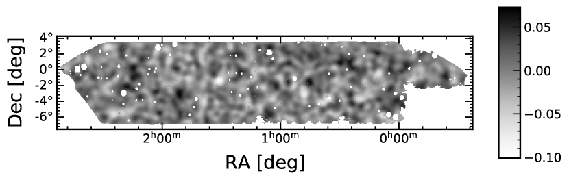
Figure 1: CMB convergence map of the d56 region, reconstructed from the combination of tSZ-cleaned ACT and Planck data [43]. The map is smoothed with a Gaussian beam with 20 arcmin for visualization purposes only. Data in the white regions are masked out regions.

3.2 DES Magnitude-limited sample (MagLim)

The DES Y3 data relies on observations taken from August 2013 to February 2016, in five broad filters, $grizY$, using the Dark Energy Camera [78]. The main catalog, referred to as Y3 GOLD, includes nearly 400 million objects over $\sim 5000\deg^{2}$ of the sky, with depth reaching S/N $\sim 10$ up to limiting magnitudes of $g=24.3$, $r=24.0$, $i=23.3$, $z=22.6$, and $Y=21.4$ [79].

In this work, we use the MagLim catalog, which is a sample defined with a magnitude cut in the $i$-band that depends linearly on photometric redshift: $i<4z+18$ [80]. This selection is based on an optimization found in [80]. Additionally, selecting $i>17.5$ removes residual stellar contamination and other bright objects. The photometric redshift is estimated from the Directional Neighborhood Fitting (DNF) algorithm [81, 79] and has been validated using cross-correlations with spectroscopic galaxies [64]. We split the catalog into 6 tomographic photometric redshift bins, spanning the range of $0.20<z<1.05$, with bin edges [0.20, 0.40, 0.55, 0.70, 0.85, 0.95, and 1.05]. In Fig. 2 we show the normalized redshift distribution for each tomographic bin.

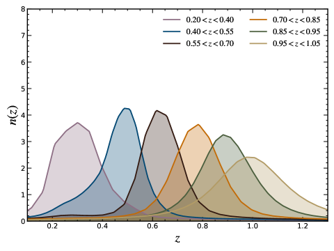
Figure 2: Normalized redshift distributions of the DES Y3 MagLim sample.

In [82] it was found that the DES galaxy number density fluctuates as a function of a series of observational conditions and survey properties. To correct this dependency in the number counts, we weighted each galaxy by the inverse of the angular selection function at that galaxy’s location [6, 63]. More information about the MagLim systematic tests and the methodology to assign weights can be found in [82] and the impact of these systematics is also investigated in Sec. 6.

3.2.1 Pixelized masks and maps

The galaxies in the MagLim catalog have an associated weight to correct for the impact of observational systematics [82]. We use these weights to construct a map of the number of sources in each pixel $\rm p$, estimated as $N_{\rm p}=\sum_{i\in\rm p}w_{i}$, where $w_{i}$ is the weight of the $i$-th galaxy. We create pixelized maps of the galaxy overdensity at a HEALPix resolution parameter $N_{\rm side}=1024$, defined by

$$\delta_{\rm p}=\bigg{(}\frac{1}{f_{\rm p}}\frac{N_{\rm p}}{\bar{n}}\bigg{)}-1,$$ (3.1)

where $\bar{n}$ denotes the mean of all number of sources in the unmasked pixels computed as

$$\bar{n}=\frac{\sum_{\rm p}N_{\rm p}}{(\sum_{\rm p}f_{\rm p})}.$$ (3.2)

The term $f_{\rm p}$ represents the DES mask, which contains information about the fraction that each pixel has been observed, the so-called fractional coverage or completeness. This mask is constructed by a series of cuts to remove astrophysical foregrounds or regions with recognized systematics, e.g., bright stars or regions with data processing issues [6]. Specifically, regions with bad quality, extreme observing conditions, areas outside the survey footprint, and pixels with fractional coverage smaller than $80\%$ are removed. More details about these cuts and the flags imposed on the MagLim sample can be found in [83, 6].

In its original resolution of $N_{\rm side}=4096$, the $f_{\rm p}$ map has values ranging from $0.8$ to $1.0$ within the DES footprint, and $0.0$ outside the footprint. We degrade the completeness map from the original resolution to $N_{\rm side}=1024$ by setting the $f_{\rm p}$ values as the mean of the higher resolution pixels. After proper masking, the MagLim sample contains $\sim 10$ million galaxies covering an area of $\sim 4100\deg^{2}$ of the sky and $\sim 1$ million galaxies in the ACT d56 region. Some of the key features of the galaxy sample are summarized in Table 1.

Redshift range	$n_{\rm gal}$ [arcmin-2]	$\ell_{\rm max}^{gg}$	$\ell_{\rm max}^{\kappa g}$
$0.20<z<0.40$	0.150	97	137
$0.40<z<0.55$	0.107	144	175
$0.55<z<0.70$	0.109	187	227
$0.70<z<0.85$	0.146	223	271
$0.85<z<0.95$	0.106	248	301
$0.95<z<1.05$	0.100	268	325

Table 1: Summary of properties of the MagLim lens sample: Redshift range, the effective number density of galaxies in units of arcmin^-2, and maximum multipole considered in the cosmological analysis for the $C_{\ell}^{gg}$ and $C_{\ell}^{\kappa g}$ (Sec 4.1).

Fig. 3 shows the MagLim overdensity map in the redshift range of $0.20<z<1.05$. The grey region shows the region of the sky that is masked, and the orange line represents the ACT d56 footprint.

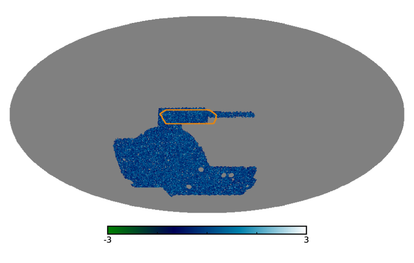
Figure 3: MagLim overdensity map for the full sample in Mollweide projection and equatorial coordinates. The grey region shows parts of the sky that are masked, and the orange line indicates the outline of the ACT d56 footprint.

4 METHODS

4.1 Angular power spectrum

The angular power spectrum estimate for a survey that covers only a fraction of the sky is affected by the mask, which introduces coupling between the different modes of the true power spectrum. We use a pseudo-$C_{\ell}$ estimator [84] implemented by NaMaster [85] to obtain an unbiased estimate of the angular power spectra. Roughly speaking, the true underlying power spectrum $C_{\ell}^{\rm true}$ is recovered in the pseudo-$C_{\ell}$ approach at every integer $\ell$ by inverting

$$C_{\ell}^{\rm obs}=\sum_{\ell^{\prime}}M_{\ell\ell^{\prime}}C_{\ell^{\prime}}^{\rm true},$$ (4.1)

where the $C_{\ell}^{\rm obs}$ is the observed power spectrum and $M$ is the so-called mode-coupling matrix. It is worth noticing that the mode coupling matrix depends solely on the mask information.

We compute the galaxy-power spectrum considering the full DES footprint, as defined by the DES mask described in Sec.3.2.1. When computing the galaxy-CMB lensing cross-power spectrum with NaMaster, it is possible to employ individual masks for each of the maps. For the DES field, we utilize the same mask used for computing the galaxy-power spectrum. For the $\kappa^{\rm CMB}$ field, we utilize the square of the mask described in Sec. 3, while also setting the masked_on_input keyword to True in NaMaster. This approach is adopted because the reconstructed CMB lensing map inherently incorporates an apodized ACT mask, given that it is applied to the CMB maps during the quadratic estimator process. We validate the mask treatment in Sec. 5.2.

When sky coverage is incomplete one needs to bin the pseudo-power spectrum and the coupling matrix. We compute the power spectra considering linearly spaced bins of width $\Delta\ell=30$ up to $\ell=3072$. However, in our analysis, we consider a conservative cut on values of $\ell$ smaller than $\ell_{\rm min}=50$ for the galaxy-power spectrum and $\ell_{\rm min}=100$ for the galaxy-CMB lensing power spectrum. We define these minimum multipoles based on the coverage of the sky and the precision of the lensing reconstruction [43], respectively.

For modeling described in Sec. 2 to be accurate, we need to ensure that our analysis encompasses scales in the linear regime, where effects such as the non-linear galaxy bias and baryonic effects on the matter power spectrum are negligible. In the DES Y3 galaxy clustering analysis [6] a scale cut corresponding to a comoving scale smaller than $R=8\leavevmode\nobreak\ h^{-1}$Mpc is imposed to exclude smaller scales on which the linear galaxy bias model breaks down. This cut corresponds to a $k_{\rm max}=1/R=0.125\leavevmode\nobreak\ h$Mpc^-1.

In our analysis, we define different scale cuts for $C_{\ell}^{gg}$ and $C_{\ell}^{\kappa g}$. For the galaxy power spectrum, we impose the scale cuts in each tomographic bin based on the “physical scale cuts”, where $\ell_{\rm max}=k_{\rm max}\chi(\bar{z})$, with a conservative $k_{\rm max}=0.08\leavevmode\nobreak\ h$Mpc^-1, hence dropping physical scales below $12.5\leavevmode\nobreak\ h^{-1}\rm{Mpc}$. Since the galaxy-CMB lensing power spectrum is less affected by the non-linearities of the galaxy bias and has expected signal-to-noise smaller than the galaxy power spectrum, we impose a more flexible scale cut for $C_{\ell}^{\kappa g}$, with $\ell_{\rm max}$ corresponding to the physical scales $k_{\rm max}$ fixed at $0.1\leavevmode\nobreak\ h\rm{Mpc}^{-1}$. These conditions led to the $\ell_{\rm max}$ values summarized in Table 1.

The galaxy power spectrum measurement has a shot noise contribution that must be subtracted. Assuming purely Poisson sampling, the “mode-coupled” shot noise can be estimated analytically [46] as

$$\tilde{N}_{\ell}=\frac{\langle m\rangle}{\bar{n}_{2}},$$ (4.2)

where $m$ is the survey mask, and $\bar{n}_{2}$ is effective number density given by

$$\bar{n}_{2}=\frac{(\sum_{i\in\rm p}w_{i})^{2}}{\Omega_{\rm pix}\sum_{\rm p}m_{\rm p}\sum_{i\in\rm p}w_{i}^{2}},$$ (4.3)

where $\Omega_{\rm pix}$ is the pixel area in units of steradians. The “mode-decoupled” bandpowers are then computed by taking the inverse of the binned mode-coupling matrix

$$N_{\ell}=\sum_{\ell^{\prime}}(M^{-1})_{\ell\ell^{\prime}}\tilde{N}_{\ell^{\prime}}.$$ (4.4)

We test the validity of the shot-noise estimate in Sec. 6.4. In the subsequent analysis, we subtract the shot-noise from the galaxy power spectrum $C_{\ell}^{gg}$, and then divide the bandpowers by the square of the pixel window function. The $C_{\ell}^{\kappa g}$ is divided by one power of the pixel window function. Finally, when comparing data with theory, we apply the appropriate binned mode-coupling matrix and binning scheme to the theoretical curves.

4.2 Covariance Matrix

In order to quantify the correlation between bandpowers in our analysis, we consider the so-called disconnected part of the covariance, that is, we assume that all fields are Gaussian distributed. We do not include the non-Gaussian covariance term in our analysis, since we consider only linear or weakly nonlinear scales, where the disconnected terms of the covariance are dominant and the non-Gaussian corrections are expected to be small [86]. In addition, the super-sample covariance term, responsible for correlations on large scales, is largely subdominant for a survey like DES Y3, as shown in [87]. This means that, for the purposes of this work, we can safely employ a Gaussian covariance.

In the absence of sky masks, the different harmonic modes are uncorrelated in the Gaussian covariance, so its computation for two fields, X and Y, reduces to the diagonal terms given by

$$\mathrm{Cov}^{XY}_{\ell\ell^{\prime}}=(\sigma^{XY}_{\ell})^{2}\delta_{\ell\ell^{\prime}},$$ (4.5)

where the error $\sigma^{XY}_{\ell}$ can be computed using

$$(\sigma^{XY}_{\ell})^{2}=\frac{1}{(2\ell+1)}[(C_{\ell}^{XX})(C_{\ell}^{YY})+(C_{\ell}^{XY})^{2}],$$ (4.6)

where the auto-power spectra terms above contain the contribution of the associated noise, $N_{\ell}$.

While the expression above is accurate for full-sky and some particular cases of partial sky [88], a sky mask introduces a non-zero correlation between different modes in the Gaussian covariance and may also affect the amplitude of the main diagonal elements. To account for these, we use the method proposed in [89, 90], implemented in NaMaster, where the covariance is computed as

$$\rm{Cov}(C_{\ell}^{\rm XY,obs}C_{\ell^{\prime}}^{\rm XY,obs})=\frac{1}{(2\ell^{\prime}+1)}[C_{(\ell}^{XX}C_{\ell^{\prime})}^{YY}\mathrm{M}_{\ell\ell^{\prime}}+C_{(\ell}^{XY}C_{\ell^{\prime})}^{YX}\mathrm{M}_{\ell\ell^{\prime}}].$$ (4.7)

The coupling matrix $\mathrm{M}_{\ell\ell^{\prime}}$ is computed based on the masks of fields $X$ and $Y$ (see [90] for further details).

The NaMaster algorithm requires the use of the underlying power spectra, $C_{\ell}^{gg},C_{\ell}^{\kappa g}$ and $C_{\ell}^{\kappa\kappa}$, for example, from the theoretical prediction that depends on parameters that we do not know a priori, such as the galaxy bias. In order to circumvent this issue and perform our analysis according to the blinding policy described in Sec. 4.4, we compute the covariance using the power spectra computed with the fiducial cosmology described in Table 2. After unblinding the data results, we update the analysis with the covariance computed with this best-fit cosmology, finding $\sim 0.3\sigma$ changes in the main result for $S_{8}$.

When computing the covariance, we consider the noise contribution of the galaxy field given by Eq. 4.4. For the CMB convergence field, we estimate the noise contribution by taking the residual between the power spectrum of the noisy ACT CMB lensing simulations [43] and the noiseless CMB lensing simulations used as input to lens the ACT CMB simulations. This approach takes into account the impact of the noise caused by the lensing reconstruction and survey geometry. As a sanity check, in section 5.3 we use lognormal mock galaxy catalogs to check the robustness of the covariance matrix computation.

Table 2: The parameters and their priors used in the analysis considering a flat $\Lambda$CDM universe. Square brackets denote a flat prior, while parentheses denote a Gaussian prior of the form $\mathcal{N}(\mu,\sigma)$. The Fiducial column shows the fiducial values we consider to construct the simulations in Sec 5.1.

Parameter	Fiducial	Prior
Cosmology
$\Omega_{\rm m}$	0.309	[0.1, 0.9]
$A_{\mathrm{s}}10^{9}$	2.19	[$0.5$, $5.0$]
$n_{\rm s}$	0.97	[0.87, 1.07]
$\Omega_{b}$	0.049	[0.03, 0.07]
$h_{0}$	0.69	[0.55, 0.91]
Linear galaxy bias
$b_{i}$	$1.5,1.8,1.8,1.9,2.3,2.3$	[0.8,3.2]
Lens magnification
$s_{i}$	0.642, 0.63 , 0.776, 0.794, 0.756, 0.896	Fixed
Lens photo-z shift and stretch
$\Delta z_{1}$	0.0	($-0.009,0.007$)
$\Delta z_{2}$	0.0	($-0.035,0.011$)
$\Delta z_{3}$	0.0	($-0.005,0.006$)
$\Delta z_{4}$	0.0	($-0.007,0.006$)
$\Delta z_{5}$	0.0	($0.002,0.007$)
$\Delta z_{6}$	0.0	($0.002,0.008$)
$\sigma z_{1}$	1.0	($0.975,0.062$)
$\sigma z_{2}$	1.0	($1.306,0.093$)
$\sigma z_{3}$	1.0	($0.870,0.054$)
$\sigma z_{4}$	1.0	($0.918,0.051$)
$\sigma z_{5}$	1.0	($1.08,0.067$)
$\sigma z_{6}$	1.0	($0.845,0.073$)

4.3 Parameter inference

In order to extract cosmological information from the measured $C_{\ell}^{gg}$ and the $C_{\ell}^{\kappa g}$, we evaluate the posterior of the parameters conditional on the data by assuming a Gaussian likelihood, $\mathcal{L}$, of the form

$$\ln\mathcal{L}(\textbf{D}|\boldsymbol{\theta})=-\frac{1}{2}[\textbf{D}-x(\boldsymbol{\theta})]^{\mathrm{T}}\mathrm{Cov}^{-1}[\textbf{D}-x(\boldsymbol{\theta})],$$ (4.8)

where D is the measured data vector, $x(\boldsymbol{\theta})$ is the theoretical prediction at parameter values $(\boldsymbol{\theta})$. The quantity $\mathrm{Cov}^{-1}$ denotes the inverse of the covariance matrix, described in Sec 4.2, and which we keep constant during parameter estimation. The posterior distribution is then proportional to the product of the likelihood and the priors

$$p(\boldsymbol{\theta}|\textbf{D})\propto\mathcal{L}(\textbf{D}|\boldsymbol{\theta})\pi(\boldsymbol{\theta}),$$ (4.9)

where $\pi(\boldsymbol{\theta})$ are the priors on the parameters of our model.

We consider a spatially flat $\Lambda$CDM cosmology, characterized by the total matter density $\Omega_{m}$, the baryonic density $\Omega_{b}$, the dimensionless Hubble parameter $h$, the amplitude of primordial scalar density perturbations $A_{s}$, and the spectral index $n_{s}$ of the power spectrum. We do not expect massive neutrinos to impact our analysis, given our scale cuts, the expected significance of the cross-correlation, and that DES Y3 clustering analysis poorly constrains the neutrino mass [63]. Therefore, we consider only massless neutrinos to speed up the computation of the matter power spectrum. The prior ranges for the parameters are listed in Table 2, and are motivated by physical constraints or by the DES Y3 analysis [6].

We sample the likelihood using the Monte Carlo Markov Chain (MCMC) sampler, implemented in the publicly available code Cobaya[91, 92]. We determine the chain convergence using a generalized version of the $R-1$ Gelman-Rubin statistic [92, 93], which we establish that the chains converge once $R-1<0.05$. We remove the first 30$\%$ of the chains from all analyses as burn-in. All the visualization of our results is done with GetDist [94].

4.4 Blinding

The results were blinded throughout the analysis until we tested the pipeline and passed all the tests for systematic effects. The tests we performed before unblinding the cosmological results are summarized below:

• First, we tested all the stages of the analysis pipeline using simulations, described in Sec. 5. We validated that we could recover the input power spectra, cosmological, and nuisance parameters of the simulations.

• Next, we used the real data to test for possible systematic contamination in our measurements. These include: 1) check the robustness of the weights applied to correct correlations in the number density map with survey properties; 2) understand and test for spurious contributions to our $C_{\ell}^{\kappa g}$ signal due possible correlated foregrounds; 3) validate the shot-noise subtraction in the $C_{\ell}^{gg}.$

• Once the above issues were well understood, we ran the parameter inference using real data under different choices in the pipeline. In this step, we looked at the blinded contours only, removing the axes when generating the figures of the parameter constraints. The real data points were not directly compared with theoretical predictions until they were unblinded.

We describe the changes done post-unblinding in Sec. 6.5.

5 SIMULATIONS AND PIPELINE VALIDATION

In this section, we apply our methodology to mock simulations to assess the validity of the power spectrum computation, covariance estimation, and the parameter constraints over the range of angular scales considered.

5.1 Lognormal Mocks

An important step before unblinding is to validate the pipeline using synthetic data with the noise levels, survey geometry, and galaxy density as in the real data. While the variance of the galaxy-CMB lensing convergence power spectrum can be captured to sufficient accuracy by Gaussian random fields, this is not realistic for the galaxy power spectrum due to the non-linear evolution of the density field [95]. On the scales we consider in our analysis, the one and the two-point function of the galaxy field can be better modeled by a field drawn from a lognormal distribution [96, 97, 98, 99].

We follow the methodology described in Sec. 3.1 of [100] to produce a set of 1000 correlated Gaussian and lognormal simulations mimicking the ACT CMB lensing field and the DES galaxy overdensity, respectively . For this, we consider the mean galaxy number density per steradian of the real data and the theoretical power spectrum computed based on the cosmological parameters, linear galaxy bias, lens magnification, and photometric redshift uncertainties listed in the “Fiducial” column of Table 2.

We draw random galaxies following a Poissonian distribution to add the shot-noise within the survey’s footprint. Then, we convert the galaxy number counts maps into galaxy overdensity maps $\delta_{g}^{\rm mock}$. Finally, we add Gaussian realizations of the CMB lensing noise [43] to the CMB lensing simulations. We account for the masks and the same pixelization scheme described in Sec 3.2.1 in the mock production.

5.2 Angular power spectrum validation

In order to validate the mask treatment in the power spectrum computation, we apply the methodology described in Sec. 4 on the 1000 lensing convergence and galaxy overdensity mock simulations with known cosmology. In Fig. 4 we show the average of the $C_{\ell}^{gg}$ (left panel) and $C_{\ell}^{\kappa g}$ (right panel) measured from these mocks, compared with the input theoretical power spectrum. We verify that both measurements, the auto and cross-power spectrum, are in good agreement with the input signal with sub-percent accuracy over the range of scales of interest. The level of agreement is much better than the measurement uncertainty for any of the bins. For clarity, the figure shows the result of the second redshift bin of the MagLim sample simulations, but these results are consistent for all redshift bins.

In addition to the mask treatment in the $C_{\ell}^{\kappa g}$ computation, we also want to test additional effects that may impact the ACT convergence reconstruction map and thus potentially bias our measurements. Such sources of bias could include, for example, the HEALPix projection of the convergence map, the mask treatment, the normalization correction in the lensing reconstruction, or any non-trivial mask effect during the lensing reconstruction. To this end, we generated 500 constrained realizations of the galaxy overdensity, which are correlated with the noiseless lensing potential maps used as the input to lens the ACT CMB simulations [43]. Then, we computed the cross-power spectrum of these galaxy simulations with the respective noisy suite of ACT lensing maps. These noisy lensing simulations accurately reflect the signal and noise properties of the ACT data. The $C_{\ell}^{\kappa g}$ obtained from this simulation suite is in agreement with the input power spectrum to within $<0.1\sigma$ (where $\sigma$ here is the error of the mean), as shown in Fig. 5.

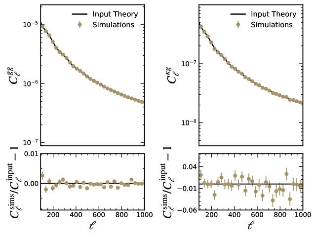
Figure 4: Comparison between the average power spectrum computed from simulations with the input power spectrum for the galaxy (left panel) and galaxy-CMB lensing (right panel) power spectrum. The error bars are divided by $\sqrt{N_{\rm{sims}}}$, where $N_{\rm{sims}}=1000$. We show the results for the second redshift bin, but are similar for all redshift bins.

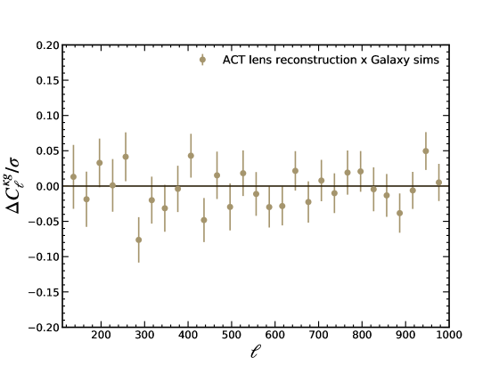
Figure 5: Test of any residual bias in the galaxy-CMB lensing power spectrum from lensing reconstruction and mask treatment. The points show the difference between the cross-power spectrum of the constrained realizations of DES galaxies and the ACT lensing simulation compared to the input, in units of the error bar of the data.

5.3 Covariance validation

In our analysis, the covariance matrix is estimated with the NaMaster algorithm, assuming a Gaussian (disconnected) approximation. When doing the parameter inference using multiple tomographic bins, we do not consider the cross-spectra between the tomographic bins. Nevertheless, we include all the cross-terms in our covariance, i.e., the cross-covariance of $C_{\ell}^{g_{i}g_{j}}$ and $C_{\ell}^{\kappa g_{i}}$. However, the resulting matrix is dominated by its diagonal components.

We checked our covariance matrix against one produced by the lognormal simulations. Fig. 6 shows the diagonals of the covariance matrix estimated using simulations and NaMaster. For both the galaxy auto-spectrum (upper panel) and galaxy-CMB lensing power spectrum (lower panel), we find that the NaMaster covariance is in very good agreement with the covariance computed directly using the simulations. For clarity, we show the result of the fifth redshift bin, but we find analogous agreement for the other bins. Thus, we conclude that the NaMaster covariance accurately recovers the power spectrum uncertainties given the impact of the survey geometry.

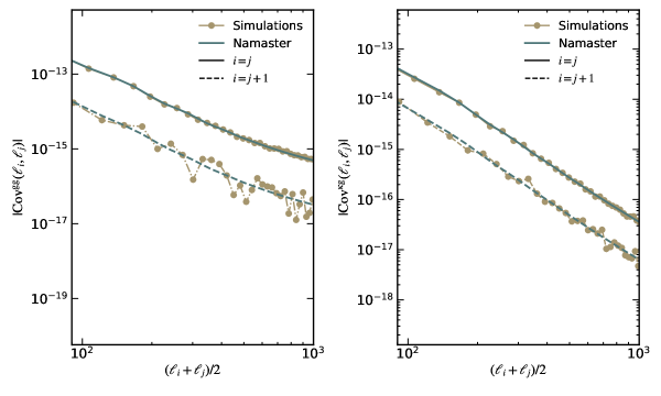
Figure 6: Comparison of the diagonal terms of the covariance matrix computed directly from the simulations and NaMaster covariances (see Section 5.3). The solid and dashed lines show the zeroth-order ($i=j$) and first-order ($i=j+1$) diagonals, respectively. For clarity, we show the covariance elements of $C_{\ell}^{gg}$ (left panel) and $C_{\ell}^{\kappa g}$ (right panel) of the fifth redshift bin, but we find similar agreement for the other bins.

5.4 Parameter estimation on mocks

We seek to constrain cosmological parameters using observations. In order to validate the parameter inference, we test the ability in recovering the input cosmological and nuisance parameters using simulations. We verify the results using the power spectra measured from two independent realizations as the data vector and also using the average of the set of simulations.

We performed a $C_{\ell}^{gg}$ and $C_{\ell}^{\kappa g}$ joint fit for the 6 photo-z bins with a total of 23 free parameters, including the galaxy bias, photo-z uncertainties, and cosmological parameters. We impose the priors shown in Table 2 for the linear galaxy bias and cosmological parameters. As our simulations do not include the photo-z uncertainties, we consider a Gaussian prior with mean-centered on zero and one respectively for the photo-z shift and stretch parameters, and width equal to the values considered in the real data shown in Table 2. We apply the same scale cuts as in the analysis of the real data. In Figure 7 we show the marginal posterior distributions for the linear galaxy bias of the six tomographic bins, $\Omega_{m}$ and $\sigma_{8}$ obtained for a given set of $C_{\ell}^{gg}$ and $C_{\ell}^{\kappa g}$ extracted from two independent realizations (yellow and blue curves) and from the average of the set of simulations (black curves). In all cases, the results are compatible with their input values, thus validating our pipeline. The small deviation from the input values seen in some of the parameters constrained from individual simulations is expected due to statistical fluctuations.

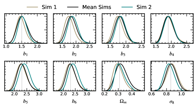
Figure 7: Synthetic parameter constraints obtained using simulations to test the pipeline. The solid curves show the marginal posterior distributions for 6 linear galaxy bias, $\sigma_{8}$ and $\Omega_{m}$ given a set of $C_{\ell}^{gg}$ and $C_{\ell}^{\kappa g}$ extracted from two independent realizations (colored lines) and from the average of the set of simulations (black curves). The dashed vertical lines depict the true values used in the simulations. The constraints from the data appear in Fig. 15.

6 ROBUSTNESS OF THE RESULTS

The Y3 MagLim sample and the ACT DR4 CMB lensing map have undergone thorough tests for various astrophysical and systematic effects in previous studies [82, 55, 71, 43]. Here, we perform additional tests to further assess the robustness of our measured bandpowers.

6.1 Weights vs deprojection

Sky contaminants such as non-cosmological sources, artifacts in the images, and other systematic effects coming from the observing conditions may change the selection function across the observed footprint or with redshift. Consequently, the observed number density of galaxies may vary according to the conditions of the survey. A detailed analysis of the impact of these survey properties or observational effects in the MagLim number density was explored in [82], which derived weights to account for correlations in the number density with survey properties. As discussed in 3.2, we apply these weights in our analysis when producing the total pixelized number counts map. A full characterization of the effect of observational systematics on the MagLim number counts is presented in [82]. Here, we perform additional tests to ensure that the systematics and the survey properties do not significantly impact our measurements.

In order to validate that the weighting applied to the number counts map is robust to correct for the effect of systematics on the galaxy-power spectrum and on the galaxy-CMB lensing power spectrum, we apply a technique called “template deprojection” [101, 85]. For that, it is assumed that the observed galaxy overdensity, $\delta^{\rm obs}$, is modeled linearly with the contaminants so that

$$\delta^{\rm obs}=\delta^{\rm true}+\alpha t,$$ (6.1)

where the "true" overdensity, $\delta^{\rm true}$, receives contributions from the template maps of the fluctuation of known contaminants, $t$, scaled by an unknown linear amplitude $\alpha$. The modes that are common to the set of systematic templates and the observed maps are removed by building a likelihood for $\delta^{\rm obs}$, considering a model for $\delta^{\rm true}$ and marginalizing over $\alpha$. This can be achieved by projecting $\delta^{\rm obs}$ onto the subspace orthogonal to $t$ and analytically accounting for the associated loss of modes when estimating the angular power spectrum. We refer the readers to the listed references for more details on the template deprojection method.

We use a set of 107 maps corresponding to DES survey properties (SP) in different photometric bands $\{g,r,i,z\}$, stellar density, and the interstellar extinction map as the contaminant templates. This set corresponds to the systematics considered in the DES Y3 Key Project. More detailed information on the construction of these maps may be found in [83] and in [82].

To evaluate the impact of these contaminants, we compare the resulting power spectra after the template deprojection from galaxy overdensity maps constructed without the weights applied to the number counts. The SP deprojection and weighting are different techniques that supposedly correct for the same effects, so we expect the deprojected power spectra of unweighted galaxy maps to be consistent with the power spectra of the weighted maps.

Fig. 8 shows the difference between the power spectrum measurements of weighted maps (our baseline measurements) and after deprojecting the contaminants of unweighted maps, in units of the statistical error. In both measurements, $C_{\ell}^{gg}$ (left panel) and $C_{\ell}^{\kappa g}$ (right panel), the deprojected $C_{\ell}$ of unweighted maps are only sub-percent different from the baseline measurements, by less than $\sim 0.3\sigma$ within the scales of interest. This consistency provides additional confidence that the SP are already accounted for by the data cuts and weighting since their effects are subdominant with respect to other sources of uncertainty.

Figure 8: Comparison of the power spectrum measurements of weighted maps (our baseline measurements) and after deprojecting the contaminants of unweighted maps, in units of statistical error. For both measurements, galaxy auto-power spectrum (left panel) and CMB lensing-galaxy power spectrum (right panel), the residual is less than $\sim 0.3\sigma$ within the scales of interest (colored lines), suggesting no significant contamination. The grey dashed lines denote the multipole range not used in our analysis.

6.2 tSZ and CIB effects

One of the major contaminants to the CMB lensing cross-correlations with tracers of large-scale structure is the tSZ effect. For this reason, in our baseline analysis, we use a CMB lensing map where tSZ has been explicitly removed (“tSZ-free”). To evaluate the impact of the tSZ effect on the CMB lensing map on our analysis, we perform an additional test by measuring the cross-correlation between the MagLim galaxies and a CMB lensing map without tSZ removal (“with-tSZ”). The aim of this test is to characterize the change in the $C_{\ell}^{\kappa g}$, as well as any potential scale dependence caused in the presence of the tSZ.

To assess the tSZ effect, we reconstruct the with-tSZ map based on ACT-only data, instead of the combination of ACT and Planck’s data used in the tSZ-free map [43]. These two maps contain slightly different noise levels. We estimate the noise level of the with-tSZ map by taking the mean difference of the auto-power spectrum of 500 ACT simulations and their input power spectrum. These simulations are built considering the same setup and reconstruction method used for the data. We use the associated noise of the field and the method described in Sec. 4.2 to compute the covariance of the $C_{\ell}^{\kappa^{\rm with-tSZ}g}$.

Figure 9 shows the difference between the $C_{\ell}^{\kappa g}$ extracted from the convergence map with tSZ and from the tSZ-free map, in units of the total error of the measurement. Although we use the tSZ-free convergence map in our baseline analysis, the power spectrum does not change significantly if we do not deproject the effect, by less than $\sim 0.3\sigma$ in the scales of interest and with no clear scale dependency. Therefore, we can conclude that even if we had used a CMB lensing map without tSZ removal, it would not significantly impact our results.

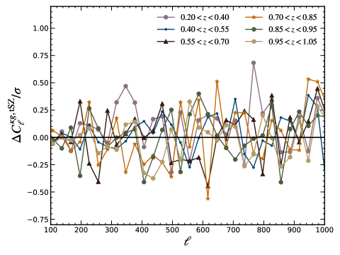
Figure 9: Difference between the $C_{\ell}^{\kappa g}$ extracted from the convergence map with tSZ and from the tSZ-free map, in units of the total error of the measurement. Although we use the tSZ-free convergence map in our baseline analysis, the power spectrum does not change significantly if we do not deproject the effect, by less than $\sim 0.3\sigma$ in the scales of interest.

Another expected bias to the galaxy-CMB lensing cross-correlations is the CIB originated dominantly from the emission from unresolved dusty star-forming galaxies. At the same time that the CIB correlates with the galaxies, its signal may leak into convergence in the lensing reconstruction [102]. However, we do not expect a strong correlation between CIB with the MagLim galaxy sample since the CIB emission is mostly sensitive to redshifts $z\sim 2$, higher than those probed by DES galaxies. The impact of the CIB in the galaxy-CMB lensing cross-correlation considering DES-like galaxies was explored in [103], finding that the CIB contamination is sub-dominant compared to the tSZ contamination (see. Fig 3 of [103]). Since our results are stable in the case of a CMB with tSZ (as shown in Fig. 9 ), we conclude that any possible bias introduced by the CIB is insignificant compared to our uncertainties.

6.3 Null-tests

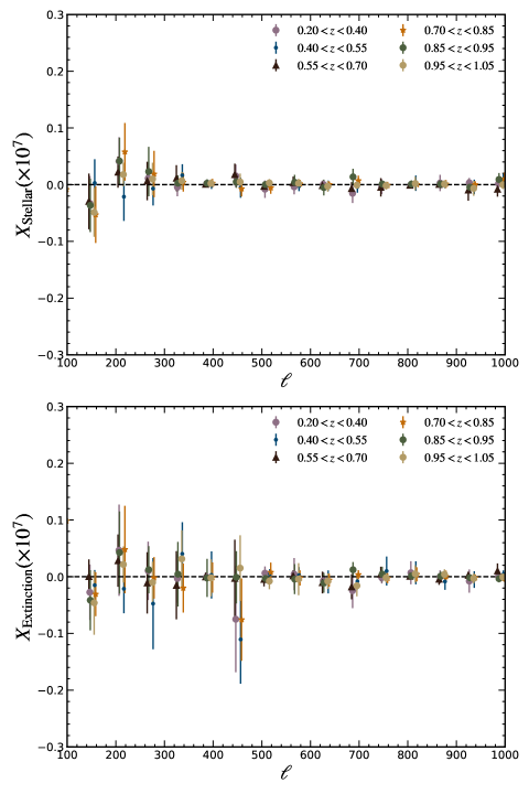
Figure 10: Contributions due to stellar contamination (upper panel) and extinction (lower panel) to the galaxy-CMB lensing cross-power spectrum, assessed by Eq. 6.2. The error bars are computed from the covariance obtained from a jackknife samples. In all cases we find no significant signal, and therefore, the null-test is consistent with zero. For clarity, the points are slightly shifted along the x-axis.

Cross-correlation between independent probes is generally less sensitive to known (and unknown) additive systematics compared to auto-correlation. However, there are systematics that can contaminate both, CMB lensing and galaxy overdensity and therefore, impact our $C_{\ell}^{\kappa g}$. For instance, the extinction of distant sources by dust in our galaxy can modulate the number counts of galaxies and add signals in CMB temperature and polarization data. The stellar density is a potential source of systematic error, as it can correlate with foregrounds that might bias lensing reconstruction and modulate galaxy number density, potentially leading to a dilution of both auto and cross-correlations [41]. In order to check the validity of our measurements against the possibility of spurious signals from contamination we compute

$$X_{S}=\frac{C_{\ell}^{\kappa S}C_{\ell}^{\delta_{g}S}}{C_{\ell}^{SS}},$$ (6.2)

where $S$ denotes the systematic map, either the stellar contamination or dust extinction. The $X_{S}$ quantity accounts for the cross-power spectrum between the systematic map and both, $\kappa$ and $\delta_{g}$, normalized by the auto-power spectrum of $S$. If our measurements are not biased by these contaminants, we would expect this signal to be consistent with zero, compared to the statistical uncertainty of the measurements. The star map is created with bright DES point sources, hereafter stellar_dens [83], and the interstellar extinction map is made following [104].

We find no evidence for contamination and Fig. 10 shows $X_{S}$ of the stellar density (upper panel) and dust extinction (lower panel) for all redshift bins. For clarity, the points are slightly shifted along the x-axis. The error bars are computed using the “delete one jackknife” (JK) covariance [105], computed using $N_{\rm{jk}}=37$ equal-area patches. Since the number of removable JK-patches is limited by the fraction of the sky, we reduced the number of $\ell$-bins when computing $X_{S}$ to obtain a more stable covariance. We have measured the $X_{S}$ with linearly spaced bins of a width of $\Delta\ell=60$, instead of the $\Delta\ell=30$ used for the baseline analysis. We use the jackknife covariance to estimate the $\chi^{2}$ with respect to the null model ($X_{S}$ = 0), and the corresponding probability-to-exceed (PTE) for the same scale cuts summarized in Table 1. The results for each case are summarized in Table 3. In all redshift bins, we find no significant signal, and therefore, the results are in agreement with the hypothesis of no systematic contribution in $C_{\ell}^{\kappa g}$.

Correlation	Photo-z bin	$\chi^{2}$/$d.o.f$	PTE ($\%$)
Stellar Density	$0.20<z<0.40$	0.46/1	49.3
	$0.40<z<0.55$	0.005/1	94.2
	$0.55<z<0.70$	0.36/2	83.3
	$0.70<z<0.85$	1.31/2	51.9
	$0.85<z<0.95$	1.22/3	74.7
	$0.95<z<1.05$	1.99/3	57.3
Correlation	Photo-z bin	$\chi^{2}/d.o.f$	PTE ($\%$)
Extinction	$0.20<z<0.40$	0.31/1	57.4
	$0.40<z<0.55$	0.31/1	57.4
	$0.55<z<0.70$	0.05/2	97.3
	$0.70<z<0.85$	0.63/2	72.6
	$0.85<z<0.95$	0.68/3	87.7
	$0.95<z<1.05$	0.84/3	83.9

Table 3: Summary of $\chi^{2}$ per degree of freedom and the PTE for the null-test defined in Eq. 6.2. The top half of the table shows the results for the stellar density, while the lower half shows the corresponding values for the extinction map.

6.4 Shot-noise subtraction

As discussed in Sec. 4.1, we subtract the shot-noise contribution to the auto-correlation power spectra using an analytical estimate given by Eq. 4.2. However, the shot-noise can deviate from this simple relation due to several effects such as super-Poissonian variance, variations in completeness, mask, and observational systematics [106].

We verify the validity of the analytical shot-noise by taking the power spectrum of random overdensity fields. To generate these fields, we randomized positions according to the completeness map, considering the same number of objects as the real galaxy sample. In essence, these randomized fields represent an independent Poisson process sampling the same smooth overdensity field. Fig. 11 shows the comparison between the shot-noise from the analytical prediction with the average of the power spectrum measured from the randomized maps. Both results are in very good agreement, within $\sim 1\%$, thus validating shot-noise subtraction in our analysis.

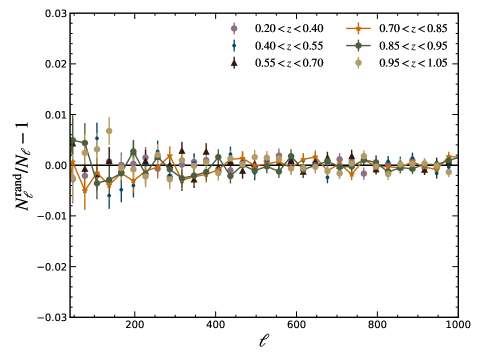
Figure 11: Comparison of the shot noise estimated analytically from Eq. 4.2 and 4.4 and from the mean of random overdensity maps with the same number of objects as the real data. The analytic estimate agrees within $\sim 1\%$ with the random estimate for all redshift bins in the scales of interest.

6.5 Unblinding

We validated the pipeline by following all the steps outlined in Section 4.4. These tests revealed no indication of systematic contamination in our measurements. Subsequently, we unblinded the cosmological parameter contour using real data and confirmed it produced a reasonable PTE with respect to the fiducial model ($>1\%$) using the covariance computed based on fiducial cosmology.

After unblinding the data, we adjusted the flat-prior range for the linear galaxy bias from [0.8-3.0] to [0.8-3.2]. We made this choice based on preliminary results that indicated the best-fit galaxy bias values of the last three redshift bins were very close to the edge of the prior. This choice doesn’t effectively change the results other than making the error bars slightly larger.

At the start of our work, our approach involved utilizing a binary mask that was generated based on non-zero values observed on a map based on the DES completeness map. However, during the latest stages of our work, we realized that the correct DES mask necessary for the harmonic space analysis should encompass the completeness of each individual pixel. In light of this, we updated the analysis to incorporate the completeness information as the DES mask, as outlined in Sec. 3.2.1. Consequently, this modification primarily affected the bandpowers at smaller scales, which were excluded from the main analysis due to scale cuts. As a result, the change on the main $S_{8}$ value was minimal, $\sim 0.1\sigma$. Nevertheless, we show the results after implementing the updated mask within our pipeline.

At this stage, the parameter inference was done using the covariance computed based on fiducial cosmology. Lastly, we updated the parameter inference by using the covariance matrix computed at the best-fit parameter values. In the subsequent sections, we present our results after accounting for these changes.

7 RESULTS

7.1 Power spectra

Fig. 12 shows the measured bandpowers, $C_{\ell}^{gg}$ (left panel) and $C_{\ell}^{\kappa g}$ (right panel), for each tomographic bin of the MagLim sample. The grey shaded region marks the range of multipoles in which the data points were discarded in the main analysis, as discussed in Sec. 4.1 and 6.5.

Before presenting the parameter constraints below, we aim to evaluate the total significance of rejecting the null hypothesis of $C_{\ell}^{\kappa g}$, i.e., the significance at which the "no-signal" hypothesis is rejected. This involves computing the significance level of rejecting the null hypothesis as

$$\chi^{2}_{\rm null}=\textbf{D}^{T}\mathrm{Cov}^{-1}\textbf{D},$$ (7.1)

where the D is the data-vector and $\mathrm{Cov}$ is the corresponding covariance matrix. Here, we consider only $C_{\ell}^{\kappa g}$ as the data vector. Then, we convert the $\chi^{2}_{\rm null}$ into a probability to exceed (PTE), given the number of degrees of freedom (dof). Finally, we express the PTE in terms of equivalent Gaussian standard deviations as the significance of the rejection of the null hypothesis. We find the significance of the rejection of the null hypothesis is 9.1$\sigma$ when considering the scale cuts of our baseline analysis, and 14.2$\sigma$ when we do not apply any scale cuts ($\ell_{\rm max}$ = $2\times N_{\rm side}$).

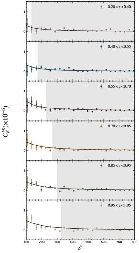
Figure 12: Extracted galaxy power spectrum (left panel) and CMB lensing-galaxy power spectrum (right panel) for each redshift bin. The grey-shaded areas highlight the range of multipoles discarded in the baseline analysis. The solid black lines represent theoretical prediction evaluated at the best-fit model developed in Sec. 7.4.

7.2 Linear Galaxy bias

The DES Y3 “3x2pt” analyses [13] found that the 2 highest redshift bins show some fluctuations in the measurements that led to a poor fit of the model. Therefore, the main 3x2pt analyses were conducted using only the first four MagLim redshift bins. We can use our $C_{\ell}^{\kappa g}$ measurements to check the consistency of the results, as we expect that CMB lensing cross-correlation would be less (or differently) contaminated by systematic effects that can plague measurements of the galaxy auto-power spectrum. However, since the degeneracy with the galaxy bias prevents the use of $C_{\ell}^{\kappa g}$ and $C_{\ell}^{gg}$ separately to constrain cosmological parameters, we can test the agreement between the two measurements by keeping the underlying cosmology fixed at the fiducial parameters listed in Table 2, while allowing the galaxy bias and parameters describing the photo-z uncertainties to vary simultaneously. Here, we essentially use the fact that $C_{\ell}^{gg}$ and $C_{\ell}^{\kappa g}$ scale with $b^{2}$ and $b$, respectively.

Fig. 13 shows the comparison of the inferred linear galaxy bias from $C_{\ell}^{gg}$ and $C_{\ell}^{\kappa g}$ individually. As expected, the cross-power spectrum has less stringent constraining power than the galaxy power spectrum. When using the $C_{\ell}^{gg}$ alone we find $b_{1}=1.51\pm 0.07$, $b_{2}=1.49^{+0.05}_{-0.06}$, $b_{3}=2.36\pm 0.07$, $b_{4}=2.29^{+0.05}_{-0.06}$, $b_{5}=2.32\pm 0.07$, and $b_{6}=2.80^{+0.08}_{-0.09}$, with the best-fit $\chi^{2}_{\rm bf}=$ 25.2 for 26 data points corresponding to a PTE of $50.7\%$. When considering the $C_{\ell}^{\kappa g}$ alone we obtain $b_{1}=1.63{\pm 0.4}$, $b_{2}=1.20{\pm 0.22}$, $b_{3}=1.88{\pm 0.35}$, $b_{4}=1.55{\pm 0.30}$, $b_{5}=2.05{\pm 0.32}$, $b_{6}=1.77{\pm 0.27}$, with $\chi^{2}_{\rm bf}=42.1$ for 31 data-points and PTE = $8.81\%$.

For all the redshift bins, the galaxy bias from $C_{\ell}^{gg}$ exhibits a preference for a higher galaxy bias compared to the $C_{\ell}^{\kappa g}$. However, given the uncertainties, we observe an acceptable agreement between the two results, except for the highest redshift bin. Other studies indicated potential issues in the measurements or modeling of the two high-redshift MagLim bins [6, 37], which can be connected to this result. However, these analyses rely on the two-point correlation function in real space, and the results largely depend on the assumed fiducial cosmology and the scale cuts applied.

Despite this result, in Sec. 7.4, we explore the stability of the cosmological constraints by using (and removing) an individual tomographic bin, finding no evidence of a significant shift. We expect to have a hint of this difference in the future using the DR6 ACT CMB lensing map which will enable us to infer a higher signal-to-noise cross-correlation.

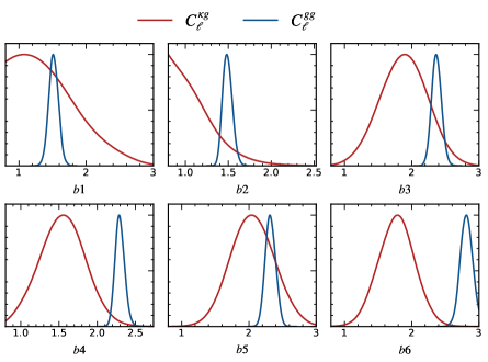
Figure 13: Constraints on linear galaxy bias for the six tomographic bins of the MagLim sample, with cosmological parameters fixed assuming the fiducial cosmology. The blue lines denote the results from galaxy-galaxy and the red lines denote the results from galaxy-CMB lensing power spectrum.

7.3 Linear growth of structure

Given the measured galaxy and galaxy-CMB lensing power spectra, we compute the linear growth factor for the six redshift bins. To this end, we use the $\hat{D}_{G}$ estimator [69], which allows one to break the degeneracy between the galaxy bias and growth structure under the assumption that both are linear and do not evolve within the selected redshift bin.

In the $\hat{D}_{G}$ computation, we account for the errors associated with the bandpowers by rewriting Eq. 2.10 as a weighted average across multipoles,

$$\hat{D}_{G}=\frac{\sum_{L}w_{L}\hat{D}_{\rm{G,L}}}{\sum_{L}w_{L}},$$ (7.2)

where $\hat{D}_{G}$ for each band power $L$ is given by

$$\hat{D}_{G,L}=\frac{(C_{L}^{\kappa g})_{\rm obs}}{(\not{C}_{L}^{\kappa g})_{\rm th}}\sqrt{\frac{(\not{C}_{L}^{gg})_{\rm th}}{(C_{L}^{gg})_{\rm obs}}}.$$ (7.3)

The weights are expressed in terms of the error of the power spectrum as

$$w_{L}^{-1}=\hat{D}_{G,L}^{2}\bigg{[}\bigg{(}\frac{\sigma(C_{L}^{\kappa g})_{\rm obs}}{(C_{L}^{\kappa g})_{\rm obs}}\bigg{)}^{2}+\frac{1}{4}\bigg{(}\frac{\sigma(C_{L}^{gg})_{\rm obs}}{(C_{L}^{gg})_{\rm obs}}\bigg{)}^{2}\bigg{]}.$$ (7.4)

The $\hat{D}_{\rm G}$ estimator is computed by taking the average of the bandpowers over a multipole range. To avoid nonlinearities, we set the maximum multipole to $\ell_{\rm max}^{gg}$, as is specified in Table 1, while the large-scale cut is set to $\ell_{\rm min}=100$ due to limitations in the $\kappa$ map. However, applying these scale cuts, the power spectra of the first redshift bin would not lie in a range suitable to compute $D_{G}$. Instead, we consider weakly-nonlinear scales up to $\ell_{\rm max}=137$ for this particular bin, but we exclude this point from the main fit below and use it solely for plotting purposes. We show in Fig. 14 the linear growth factor estimated for each tomographic bin with the corresponding $1\sigma$ error bar. The error bars are estimated from the dispersion of the $\hat{D}_{\rm G}$ computed using the auto- and cross-spectra of the correlated simulations described in Sec. 5.1.

From the growth factor estimated in each redshift bin, we can assess the evolution of growth assuming that the theoretical growth function $D_{G}^{\rm fid}(z)$ scale linearly with a redshift-independent amplitude $A_{D}$. Thus, $A_{D}$ probes the growth function with respect to the fiducial cosmology and can be estimated by minimizing the following $\chi^{2}$

$$\chi^{2}=\sum_{ij}^{6}(\hat{D}_{G}(z_{i})-A_{D}D_{G}^{\rm fid}(z_{i}))\mathrm{Cov}^{-1}_{ij}(\hat{D}_{G}(z_{j})-A_{D}D_{G}^{\rm fid}(z_{j})).$$ (7.5)

We use the MCMC approach to fit $A_{D}$, simultaneously varying both $A_{D}$ and the photo-z uncertainties ($\Delta z$ and $\sigma_{z}$) over the priors specified in Table 2. In this process, we keep the cosmological parameters fixed at their fiducial values. We set a flat prior for the parameter $A_{D}$, ranging from 0.1 to 3. The covariance is estimated from the $\hat{D}_{G}$ computed using the simulations. We obtain $A_{D}$= 0.87$\pm$ 0.14, when we consider the estimates of the five redshift bins, shown as the filled points in Fig 14. We show in Fig. 14 the fit of the growth amplitude in its $1\sigma$ confidence interval as the blue line and bands, respectively. The obtained value is within $1\sigma$ of the expected value in the fiducial case, $A_{D}=1$. Also, this result is in agreement with similar analyses using other CMB lensing and galaxy samples spanning different redshift ranges [69, 39, 40, 42, 107].

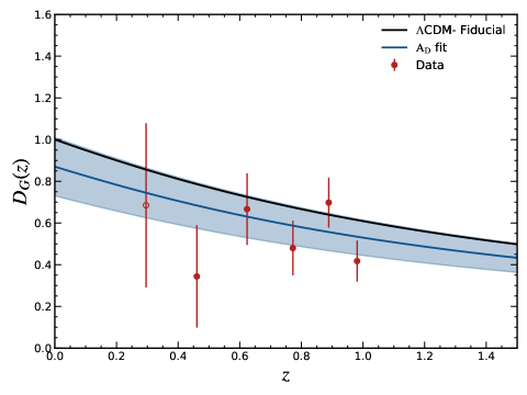
Figure 14: The linear growth factor of each tomographic bin estimated with the $\hat{D}_{\rm G}$ statistic (Eq. 7.2) that uses the combination of the galaxy and CMB-lensing-galaxy power spectrum. The red points correspond to the $\hat{D}_{\rm G}$ estimated from the data within the scale range described in Sec 7.3. The open point at $z\sim 0.29$ corresponds to the constraint using the weakly non-linear scales described in the text and is not included to fit the growth amplitude $A_{D}$, which is shown by the blue line. The blue band represents the $1\sigma$ confidence interval on the best-fit amplitude $A_{D}$, assuming the fiducial cosmology shown in the solid black line.

7.4 Cosmological Constraints

We next fit cosmological parameters to our measurements. For these fits, we sample the posterior simultaneously varying the galaxy bias, the photo-z uncertainties (i.e. $\Delta_{z}$ and $\sigma_{z}$), and the flat-$\Lambda$CDM parameters: $\Omega_{m}$, $\Omega_{b}$, $n_{s}$, $A_{s}$, and $h$. In total, this inference marginalizes over 23 parameters with prior ranges listed in Table 2. Typically LSS data is especially sensitive to $\Omega_{m}$ and to the combination

$$S_{8}\equiv\sigma_{8}\sqrt{\frac{\Omega_{m}}{0.3}},$$ (7.6)

which we are interested in placing constraints.

Figure 15 shows the constraints on the $\Omega_{m}$ and $S_{8}$ from the measured $C_{\ell}^{gg}$ and $C_{\ell}^{\kappa g}$ of the 6 tomographic bins of the MagLim sample. We find that the marginalized 68$\%$ C.L. mean values (best-fit values inside parentheses) are:

• $\Omega_{m}=0.277^{+0.029}_{-0.034}(0.26)$;

• $S_{8}=0.751^{+0.046}_{-0.048}(0.73)$.

The best-fit model has $\chi^{2}=48.7$ for 57 dof, corresponding to a PTE 77.4$\%$.

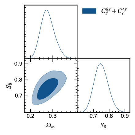
Figure 15: Constraints on $\Omega_{m}$ and $S_{8}$ obtained from the joint $C_{\ell}^{gg}$ and $C_{\ell}^{\kappa g}$ of the six tomographic redshift bins of the sample. Both $68\%$ and $95\%$ credible levels are shown.

To ensure the consistency of the results, we repeat the analysis considering various combinations of data. We perform the parameter constraints considering the following setups:

• The measurements of each individual photo-z bin.

• The measurements of 5 photo-z bins, excluding one MagLim photo-z bin at a time.

• The combination of the 4 lowest redshift bins, i.e., removing the two highest photo-z bins from the analysis.

Fig.16 shows the $1\sigma$ uncertainty on $S_{8}$ and $\Omega_{m}$ for the different scenarios described above. As a comparison, we also show the result of the baseline analysis presented highlighted in red. The largest parameter shift towards lower $S_{8}$ is found when we use only measurements from the second photo-z bin to establish constraints on the cosmological parameters; on the other hand, using the fifth photo-z bin shifts the $S_{8}$ to higher values than the baseline result. However, these constraints have visibly larger uncertainties in both cases and the shifts are less than $1\sigma$ different from the baseline result. It is worth noticing that in Fig. 14 is possible to see a similar behavior, in which the growth rate of the second (and of the fifth) photo-z bin is relatively lower (higher) than the other points. Given Fig. 16, this is not a surprising result since the $D_{G}$ scales with $S_{8}$ and $\Omega_{m}$ as well. In addition, the results are stable when removing one of the photo-z bins at a time. Therefore, the parameter constraints for all these setups are consistent with the baseline result indicating an internal consistency of the baseline data choice.

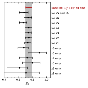
(a)

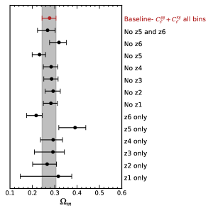
(b)

Figure 16: Summary of the constraints on $S_{8}=\sigma_{8}(\Omega_{m}/0.3)^{0.5}$ (left panel) and $\Omega_{m}$ (right panel) and their robustness against different setups in the data combination (see Section 7.4 for more details). The red dot denotes the baseline result.

Recent studies using the two-point information of the DES Y3 MagLim sample also add constraints on $S_{8}$, including the galaxy clustering and galaxy-galaxy lensing [6] ($S_{8}=0.778^{+0.037}_{-0.031}$) and the 3x2pt [63] ($S_{8}=0.776\pm 0.017$). In [37], $S_{8}$ is derived from the cross-correlation between MagLim galaxies and DES Y3 shear with the CMB lensing from Planck and SPT ($S_{8}=0.736^{+0.032}_{-0.028}$), while [108] consider the combination of the 2-point correlation function between SPT CMB-lensing, galaxy positions, and galaxy lensing ($S_{8}=0.792\pm 0.012$). Despite the fact that these analyses use different combinations of data and employ real-space correlation functions, which makes it difficult to compare their analysis choices with ours in harmonic space, our results are statistically consistent with all of them.

Other studies that rely on late-time data also suggest a lower $S_{8}$ value compared to what is inferred from CMB data within the context of $\Lambda$CDM. In particular, the analysis of the TT-TE-EE- and low-E polarization of the Planck satellite (Planck TT+TE+EE+lowE) found $S_{8}=0.834\pm 0.016$ [1], which is $\sim 1.7\sigma$ different from our results when adding the statistical uncertainties in quadrature. Interestingly, analysis of the CMB lensing from Planck [18] and, more recently, from ACT [21, 20], also reveals a $S_{8}$ value consistent with the CMB constraints, suggesting that tracers at higher redshifts and probing larger scales tend to prefer higher $S_{8}$ than the probes at lower redshifts. In Fig. 17 we summarize the comparison of our 1D marginalised $S_{8}$ parameter against these measurements.

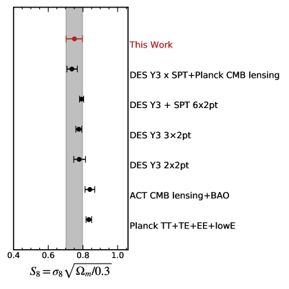
Figure 17: Comparison of measurement of $S_{8}$ from our analysis with other measurements using DES Y3 data [37, 108, 63, 6], ACT CMB lensing + BAO [20], and primordial CMB from Planck [1], though note that the DES points here include marginalization over the sum of neutrino masses.

Our results are also in agreement with other CMB-lensing cross-correlation studies, such as with the unWISE ($S_{8}=0.784\pm 0.015$) [47], DESI ($S_{8}=0.73\pm 0.03$) [48], and KiDS ($S_{8}=0.64\pm 0.08$) [36] data. The results are also consistent with [46], who reported a low $S_{8}$ value ($S_{8}=0.7781\pm 0.0094$) in comparison to CMB constraints through the cross-correlation of Planck CMB lensing with various galaxy surveys. However, their results exhibited higher $S_{8}$ when excluding shear measurements ($0.825\pm 0.023$).

It remains unclear whether the observed discrepancy in the $S_{8}$ values measured from the CMB and those derived from the late universe is due to a physical reason, an unaccounted for systematics, or due to a statistical fluctuation. It is thus important to emphasize that our analysis relies on a few assumptions. We assume validity of the model in the linear regime so that the galaxy overdensity is connected to the matter overdensity by a linear, deterministic, and scale-independent galaxy bias. However, even applying conservative scale cuts to ensure linearity, this relationship may no longer be accurate if there is a stochastic component in the galaxy density, which could be caused by various observational and astrophysical factors, such as discrete sampling and physical effects on galaxy formation other than those from the local density field [109]. To account for these potential effects, it would be necessary to increase the complexity of the model. Nevertheless, due to the uncertainties in our measurements, it is unlikely that we would be able to draw a conclusive result even with an improved model. Therefore, we leave this for future work.

8 SUMMARY

We have presented the first analysis in harmonic space of the cross-correlation between the galaxy density fluctuations from DES Y3 MagLim galaxies and CMB lensing cross-correlation. We use the CMB convergence map from the fourth ACT data release. This measurement, when combined with the galaxy power spectrum, helps to break the degeneracy between the galaxy bias and cosmological parameters. We have derived cosmological constraints by considering a tomographic approach, with six redshift bins spanning from $z=0.20$ to $1.05$.

Our pipeline has been extensively validated and we carried out several systematic checks (Sec.5 and 6), in which we found no significant evidence of unaccounted contamination in our measurements within the range of scales we use. Initially, we performed the analysis under a blinding procedure described in 4.4. After applying very conservative cuts to ensure our data lies in the linear regime, we rejected the null hypothesis of no correlation at 9.1$\sigma$. The bandpowers measurements are displayed in Fig. 12.

We use our measurements to constrain cosmology under different scenarios. First, we fixed the cosmology at the fiducial values and checked the consistency of the linear galaxy bias constrained from the $C_{\ell}^{\kappa g}$ and from the $C_{\ell}^{gg}$ data. The main result is displayed in Fig. 13 and indicates a acceptable concordance in all redshift bins, with the exception of the highest redshift bin. In this particular bin, we observe an indication of a potential discrepancy between the linear galaxy bias derived from our two measurements. Nevertheless, when removing this particular redshift bin to place constraints on $S_{8}$, we did not observe any significant impact on the results.

Next, we investigated the linear growth rate of the structures at different redshifts by employing the galaxy bias-independent $D_{G}$ estimator defined in Sec. 7.3. The main result is shown in Fig. 14. Given the growth measurements at each redshift, we constrain the parameter $A_{D}$, which represents the total amplitude of the linear growth with respect to the fiducial cosmology. We find $A_{D}=0.87\pm 0.14$, consistent with the expected value of the fiducial model, ($A_{D}=1$). Measuring $D_{G}$ tomographically is a possible way to investigate whether a preferred lower or higher $S_{8}$ value exists within a specific redshift range. This approach is motivated by the fact that certain analyses with late-time data suggest lower values of the clustering amplitude compared to the constraints imposed by primordial CMB. Due to the data limitations and the conservative scale cuts applied, we are not able to place constraints strong enough to further examine if there is a preferred trend of the $D_{G}$ evolution. This approach would significantly benefit from the use of a convergence CMB lensing map with improved overlap and noise levels, such as the latest ACT data release 6 [21, 20] that almost entirely overlaps with the DES region [110].

Finally, we vary the cosmological and astrophysical parameters to place constraints on $\Omega_{m}$ and $S_{8}$. In $\Lambda$CDM, we find at $68\%$ C.L $\Omega_{m}=0.277^{+0.029}_{-0.034}$, and $S_{8}=0.751^{+0.046}_{-0.048}$. Our main result is shown in Figure 15. We find that our $S_{8}$ constraints are slightly lower with respect to Planck TT+TE+EE+lowE at the $\sim 1.7\sigma$ level when adding the statistical uncertainties in quadrature. Our result is also consistent with other studies [63, 37, 6, 47, 48, 36]. We perform a number of internal consistency tests to assess the stability of the main result. We conducted several internal consistency tests to evaluate the robustness of our main result. A summary of these tests is presented in Fig. 16.

The current discrepancy between the inferred value of $S_{8}$ from the CMB and from some late Universe observations emphasizes the need for testing the $\Lambda$CDM model and systematic effects through various methods, datasets, and pipelines. Our study demonstrates the ability to constrain cosmology using the combination of the galaxy power spectrum and the CMB lensing- galaxy cross-power spectrum. In a companion paper [111], we explore the parameter constraint using the cross-correlation between ACT DR4 CMB lensing and DES Y3 shear data, which is also sensitive to the amplitude of large-scale structure parameter $\sigma_{8}$. Furthermore, the next data releases of galaxy surveys such as the DES, HSC, DESI, and new CMB lensing maps such as from AdvACT and SPT-3G will tighten the parameter constraints and help us to understand the history of the cosmic structure growth. This will be especially valuable if one can demonstrate that the systematic effects are well controlled, even with increased precision. In the future, a comprehensive cross-correlation analysis will be even more stringent using data from upcoming surveys such as the Vera Rubin Observatory Legacy Survey, Euclid mission , the Nancy G. Roman Space Telescope, Simons Observatory, and CMB-S4. However, accurate theoretical modeling is crucial for achieving this goal. Although we have adopted conservative scale cuts and do not extend the analysis to include mildly-small scales, a comprehensive understanding of effects significant in this regime (e.g., nonlinear galaxy bias, baryonic effects) will be essential to performing precision cosmology and is something to be addressed in a higher signal-to-noise measurement using ACT DR6 cross-correlation studies [110].

References

- [1] N. Aghanim, Y. Akrami, M. Ashdown, J. Aumont, C. Baccigalupi, M. Ballardini et al., Planck 2018 results-VI. Cosmological parameters, Astronomy & Astrophysics 641 (2020) A6.
- [2] A. Lewis and A. Challinor, Weak gravitational lensing of the CMB, Physics Reports 429 (2006) 1.
- [3] A. Albrecht, G. Bernstein, R. Cahn, W.L. Freedman, J. Hewitt, W. Hu et al., Report of the dark energy task force, arXiv preprint astro-ph/0609591 (2006) .
- [4] B. Flaugher, H. Diehl, K. Honscheid, T. Abbott, O. Alvarez, R. Angstadt et al., The Dark Energy Camera, The Astronomical Journal 150 (2015) 150.
- [5] T. Abbott, A. Alarcon, S. Allam, P. Andersen, F. Andrade-Oliveira, J. Annis et al., Cosmological constraints from multiple probes in the dark energy survey, Physical review letters 122 (2019) 171301.
- [6] A. Porredon, M. Crocce, J. Elvin-Poole, R. Cawthon, G. Giannini, J. De Vicente et al., Dark Energy Survey Year 3 results: Cosmological constraints from galaxy clustering and galaxy-galaxy lensing using the MagLim lens sample, Physical Review D 106 (2022) 103530.
- [7] T. Abbott, M. Adamow, M. Aguena, S. Allam, A. Amon, J. Annis et al., The Dark Energy Survey Data Release 2, The Astrophysical Journal Supplement Series 255 (2021) 20.
- [8] C. Hikage, M. Oguri, T. Hamana, S. More, R. Mandelbaum, M. Takada et al., Cosmology from cosmic shear power spectra with Subaru Hyper Suprime-Cam first-year data, Publications of the Astronomical Society of Japan 71 (2019) 43.
- [9] T. Hamana, M. Shirasaki, S. Miyazaki, C. Hikage, M. Oguri, S. More et al., Cosmological constraints from cosmic shear two-point correlation functions with HSC survey first-year data, Publications of the Astronomical Society of Japan 72 (2020) 16.
- [10] S. Joudaki, C. Blake, A. Johnson, A. Amon, M. Asgari, A. Choi et al., KiDS-450+ 2dFLenS: Cosmological parameter constraints from weak gravitational lensing tomography and overlapping redshift-space galaxy clustering, Monthly Notices of the Royal Astronomical Society 474 (2018) 4894.
- [11] E. van Uitert, B. Joachimi, S. Joudaki, A. Amon, C. Heymans, F. Köhlinger et al., KiDS+ GAMA: cosmology constraints from a joint analysis of cosmic shear, galaxy–galaxy lensing, and angular clustering, Monthly Notices of the Royal Astronomical Society 476 (2018) 4662.
- [12] C. Heymans, E. Grocutt, A. Heavens, M. Kilbinger, T.D. Kitching, F. Simpson et al., CFHTLenS tomographic weak lensing cosmological parameter constraints: Mitigating the impact of intrinsic galaxy alignments, Monthly Notices of the Royal Astronomical Society 432 (2013) 2433.
- [13] T. Abbott, F.B. Abdalla, A. Alarcon, J. Aleksić, S. Allam, S. Allen et al., Dark Energy Survey year 1 results: Cosmological constraints from galaxy clustering and weak lensing, Physical Review D 98 (2018) 043526.
- [14] T. Tröster, A.G. Sánchez, M. Asgari, C. Blake, M. Crocce, C. Heymans et al., Cosmology from large-scale structure-Constraining CDM with BOSS, Astronomy & Astrophysics 633 (2020) L10.
- [15] C. Heymans, T. Tröster, M. Asgari, C. Blake, H. Hildebrandt, B. Joachimi et al., KiDS-1000 Cosmology: Multi-probe weak gravitational lensing and spectroscopic galaxy clustering constraints, Astronomy & Astrophysics 646 (2021) A140.
- [16] M. Asgari, C.-A. Lin, B. Joachimi, B. Giblin, C. Heymans, H. Hildebrandt et al., KiDS-1000 cosmology: Cosmic shear constraints and comparison between two point statistics, Astronomy & Astrophysics 645 (2021) A104.
- [17] D.E. Survey, K.-D.S. Collaboration, T. Abbott, M. Aguena, A. Alarcon, O. Alves et al., DES Y3+ KiDS-1000: Consistent cosmology combining cosmic shear surveys, arXiv preprint arXiv:2305.17173 (2023) .
- [18] N. Aghanim, Y. Akrami, M. Ashdown, J. Aumont, C. Baccigalupi, M. Ballardini et al., Planck 2018 results-VIII. Gravitational lensing, Astronomy & Astrophysics 641 (2020) A8.
- [19] Z. Pan, F. Bianchini, W. Wu, P. Ade, Z. Ahmed, E. Anderes et al., A measurement of gravitational lensing of the cosmic microwave background using spt-3g 2018 data, arXiv preprint arXiv:2308.11608 (2023) .
- [20] M.S. Madhavacheril, F.J. Qu, B.D. Sherwin, N. MacCrann, Y. Li, I. Abril-Cabezas et al., The Atacama Cosmology Telescope: DR6 Gravitational Lensing Map and Cosmological Parameters, arXiv preprint arXiv:2304.05203 (2023) .
- [21] F.J. Qu, B.D. Sherwin, M.S. Madhavacheril, D. Han, K.T. Crowley, I. Abril-Cabezas et al., The Atacama Cosmology Telescope: A Measurement of the DR6 CMB Lensing Power Spectrum and its Implications for Structure Growth, arXiv preprint arXiv:2304.05202 (2023) .
- [22] Ž. Ivezić, S.M. Kahn, J.A. Tyson, B. Abel, E. Acosta, R. Allsman et al., LSST: from science drivers to reference design and anticipated data products, The Astrophysical Journal 873 (2019) 111.
- [23] A. Aghamousa, J. Aguilar, S. Ahlen, S. Alam, L.E. Allen, C.A. Prieto et al., The DESI experiment part I: science, targeting, and survey design, arXiv preprint arXiv:1611.00036 (2016) .
- [24] O. Doré, J. Bock, M. Ashby, P. Capak, A. Cooray, R. de Putter et al., Cosmology with the SPHEREX all-sky spectral survey, arXiv preprint arXiv:1412.4872 (2014) .
- [25] R. Laureijs, J. Amiaux, S. Arduini, J.-L. Augueres, J. Brinchmann, R. Cole et al., Euclid definition study report, arXiv preprint arXiv:1110.3193 (2011) .
- [26] D. Spergel, N. Gehrels, C. Baltay, D. Bennett, J. Breckinridge, M. Donahue et al., Wide-field infrarred survey telescope-astrophysics focused telescope assets WFIRST-AFTA 2015 report, arXiv preprint arXiv:1503.03757 (2015) .
- [27] B.A. Benson, P. Ade, Z. Ahmed, S. Allen, K. Arnold, J. Austermann et al., SPT-3G: a next-generation cosmic microwave background polarization experiment on the South Pole telescope, in Millimeter, Submillimeter, and Far-Infrared Detectors and Instrumentation for Astronomy VII, vol. 9153, pp. 552–572, SPIE, 2014.
- [28] P. Ade, J. Aguirre, Z. Ahmed, S. Aiola, A. Ali, D. Alonso et al., The Simons Observatory: science goals and forecasts, Journal of Cosmology and Astroparticle Physics 2019 (2019) 056.
- [29] K. Abazajian, G. Addison, P. Adshead, Z. Ahmed, S.W. Allen, D. Alonso et al., CMB-S4 decadal survey APC white paper, arXiv preprint arXiv:1908.01062 (2019) .
- [30] N. Hand, A. Leauthaud, S. Das, B.D. Sherwin, G.E. Addison, J.R. Bond et al., First measurement of the cross-correlation of CMB lensing and galaxy lensing, Physical Review D 91 (2015) 062001.
- [31] J. Liu and J.C. Hill, Cross-correlation of Planck CMB lensing and CFHTLenS galaxy weak lensing maps, Physical Review D 92 (2015) 063517.
- [32] A. Nicola, A. Refregier and A. Amara, Integrated approach to cosmology: Combining CMB, large-scale structure, and weak lensing, Physical Review D 94 (2016) 083517.
- [33] Y. Omori, E. Baxter, C. Chang, D. Kirk, A. Alarcon, G. Bernstein et al., Dark Energy Survey Year 1 Results: Cross-correlation between Dark Energy Survey Y1 galaxy weak lensing and South Pole Telescope+ P l a n c k CMB weak lensing, Physical Review D 100 (2019) 043517.
- [34] T. Namikawa, Y. Chinone, H. Miyatake, M. Oguri, R. Takahashi, A. Kusaka et al., Evidence for the cross-correlation between cosmic microwave background polarization lensing from polarbear and cosmic shear from subaru hyper suprime-cam, The Astrophysical Journal 882 (2019) 62.
- [35] G.A. Marques, J. Liu, K.M. Huffenberger and J.C. Hill, Cross-correlation between Subaru Hyper Suprime-Cam Galaxy Weak Lensing and Planck Cosmic Microwave Background Lensing, The Astrophysical Journal 904 (2020) 182.
- [36] N.C. Robertson, D. Alonso, J. Harnois-Déraps, O. Darwish, A. Kannawadi, A. Amon et al., Strong detection of the CMB lensing and galaxy weak lensing cross-correlation from ACT-DR4, Planck Legacy, and KiDS-1000, Astronomy & Astrophysics 649 (2021) A146.
- [37] DES & SPT Collaborations collaboration, Joint analysis of Dark Energy Survey Year 3 data and CMB lensing from SPT and . II. Cross-correlation measurements and cosmological constraints, Phys. Rev. D 107 (2023) 023530.
- [38] F. Bianchini, P. Bielewicz, A. Lapi, J. Gonzalez-Nuevo, C. Baccigalupi, G. De Zotti et al., Cross-correlation between the CMB lensing potential measured by Planck and high-z submillimeter galaxies detected by the Herschel-ATLAS survey, The Astrophysical Journal 802 (2015) 64.
- [39] F. Bianchini and C.L. Reichardt, Constraining Gravity at Large Scales with the 2MASS Photometric Redshift Catalog and Planck Lensing, The Astrophysical Journal 862 (2018) 81.
- [40] Y. Omori, T. Giannantonio, A. Porredon, E. Baxter, C. Chang, M. Crocce et al., Dark Energy Survey Year 1 Results: Tomographic cross-correlations between Dark Energy Survey galaxies and CMB lensing from South Pole Telescope+ Planck, Physical Review D 100 (2019) 043501.
- [41] A. Krolewski, S. Ferraro, E.F. Schlafly and M. White, unWISE tomography of Planck CMB lensing, Journal of Cosmology and Astroparticle Physics 2020 (2020) 047.
- [42] G.A. Marques and A. Bernui, Tomographic analyses of the CMB lensing and galaxy clustering to probe the linear structure growth, Journal of Cosmology and Astroparticle Physics 2020 (2020) 052.
- [43] O. Darwish, M.S. Madhavacheril, B.D. Sherwin, S. Aiola, N. Battaglia, J.A. Beall et al., The Atacama Cosmology Telescope: a CMB lensing mass map over 2100 square degrees of sky and its cross-correlation with BOSS-CMASS galaxies, Monthly Notices of the Royal Astronomical Society 500 (2021) 2250.
- [44] E. Kitanidis and M. White, Cross-correlation of Planck CMB lensing with DESI-like LRGs, Monthly Notices of the Royal Astronomical Society 501 (2021) 6181.
- [45] Q. Hang, S. Alam, J.A. Peacock and Y.-C. Cai, Galaxy clustering in the DESI Legacy Survey and its imprint on the CMB, Monthly Notices of the Royal Astronomical Society 501 (2021) 1481.
- [46] C. García-García, J.R. Zapatero, D. Alonso, E. Bellini, P.G. Ferreira, E.-M. Mueller et al., The growth of density perturbations in the last 10 billion years from tomographic large-scale structure data, arXiv preprint arXiv:2105.12108 (2021) .
- [47] A. Krolewski, S. Ferraro and M. White, Cosmological constraints from unWISE and Planck CMB lensing tomography, Journal of Cosmology and Astroparticle Physics 2021 (2021) 028.
- [48] M. White, R. Zhou, J. DeRose, S. Ferraro, S.-F. Chen, N. Kokron et al., Cosmological constraints from the tomographic cross-correlation of DESI Luminous Red Galaxies and Planck CMB lensing, Journal of Cosmology and Astroparticle Physics 2022 (2022) 007.
- [49] B.D. Sherwin, S. Das, A. Hajian, G. Addison, J.R. Bond, D. Crichton et al., The Atacama Cosmology Telescope: Cross-correlation of cosmic microwave background lensing and quasars, Physical Review D 86 (2012) 083006.
- [50] J. Geach, R. Hickox, L. Bleem, M. Brodwin, G. Holder, K. Aird et al., A direct measurement of the linear bias of mid-infrared-selected quasars at z 1 using cosmic microwave background lensing, The Astrophysical Journal Letters 776 (2013) L41.
- [51] C. Doux, M. Penna-Lima, S.D. Vitenti, J. Tréguer, E. Aubourg and K. Ganga, Cosmological constraints from a joint analysis of cosmic microwave background and spectroscopic tracers of the large-scale structure, Monthly Notices of the Royal Astronomical Society 480 (2018) 5386.
- [52] G. Holder, M. Viero, O. Zahn, K. Aird, B. Benson, S. Bhattacharya et al., A CMB lensing mass map and its correlation with the cosmic infrared background, arXiv preprint arXiv:1303.5048 (2013) .
- [53] A. Van Engelen, B.D. Sherwin, N. Sehgal, G.E. Addison, R. Allison, N. Battaglia et al., The Atacama Cosmology Telescope: lensing of CMB temperature and polarization derived from cosmic infrared background cross-correlation, The Astrophysical Journal 808 (2015) 7.
- [54] Y. Cao, Y. Gong, C. Feng, A. Cooray, G. Cheng and X. Chen, Cross-correlation of Far-infrared Background Anisotropies and CMB Lensing from Herschel and Planck Satellites, The Astrophysical Journal 901 (2020) 34.
- [55] S. Aiola, E. Calabrese, L. Maurin, S. Naess, B.L. Schmitt, M.H. Abitbol et al., The Atacama Cosmology Telescope: DR4 maps and cosmological parameters, Journal of Cosmology and Astroparticle Physics 2020 (2020) 047.
- [56] J.N. Fry and E. Gaztanaga, Biasing and hierarchical statistics in large-scale structure, Astrophys. J. 413 (1993) 447.
- [57] E. Krause, X. Fang, S. Pandey, L. Secco, O. Alves, H. Huang et al., Dark Energy Survey Year 3 Results: Multi-Probe Modeling Strategy and Validation, arXiv preprint arXiv:2105.13548 (2021) .
- [58] E. Turner, The effect of undetected gravitational lenses on statistical measures of quasar evolution, The Astrophysical Journal 242 (1980) L135.
- [59] P. Schneider, The number excess of galaxies around high redshift quasars, Astronomy and Astrophysics 221 (1989) 221.
- [60] R. Moessner and B. Jain, Angular cross-correlation of galaxies: a probe of gravitational lensing by large-scale structure, Monthly Notices of the Royal Astronomical Society 294 (1998) L18.
- [61] J. Elvin-Poole, N. Maccrann, S. Everett, J. Prat, E. Rykoff, J. De Vicente et al., Dark Energy Survey Year 3 results: Magnification modeling and impact on cosmological constraints from galaxy clustering and galaxy-galaxy lensing, arXiv preprint arXiv:2209.09782 (2022) .
- [62] J. DeRose, R. Wechsler, M. Becker, E. Rykoff, S. Pandey, N. MacCrann et al., Dark Energy Survey Year 3 results: cosmology from combined galaxy clustering and lensing–validation on cosmological simulations, arXiv preprint arXiv:2105.13547 (2021) .
- [63] T. Abbott, M. Aguena, A. Alarcon, S. Allam, O. Alves, A. Amon et al., Dark energy survey year 3 results: cosmological constraints from galaxy clustering and weak lensing, Physical Review D 105 (2022) 023520.
- [64] R. Cawthon, J. Elvin-Poole, A. Porredon, M. Crocce, G. Giannini, M. Gatti et al., Dark Energy Survey Year 3 Results: Calibration of Lens Sample Redshift Distributions using Clustering Redshifts with BOSS/eBOSS, arXiv preprint arXiv:2012.12826 (2020) .
- [65] D.N. Limber, The Analysis of Counts of the Extragalactic Nebulae in Terms of a Fluctuating Density Field., The Astrophysical Journal 117 (1953) 134.
- [66] A. Lewis, A. Challinor and A. Lasenby, Efficient computation of cosmic microwave background anisotropies in closed Friedmann-Robertson-Walker models, The Astrophysical Journal 538 (2000) 473.
- [67] R. Takahashi, M. Sato, T. Nishimichi, A. Taruya and M. Oguri, Revising the halofit model for the nonlinear matter power spectrum, The Astrophysical Journal 761 (2012) 152.
- [68] N.E. Chisari, D. Alonso, E. Krause, C.D. Leonard, P. Bull, J. Neveu et al., Core cosmology library: Precision cosmological predictions for LSST, The Astrophysical Journal Supplement Series 242 (2019) 2.
- [69] T. Giannantonio, P. Fosalba, R. Cawthon, Y. Omori, M. Crocce, F. Elsner et al., CMB lensing tomography with the DES Science Verification galaxies, Monthly Notices of the Royal Astronomical Society 456 (2016) 3213.
- [70] R. Thornton, P. Ade, S. Aiola, F. Angile, M. Amiri, J. Beall et al., The Atacama cosmology telescope: the polarization-sensitive ACTPol instrument, The Astrophysical Journal Supplement Series 227 (2016) 21.
- [71] S.K. Choi, M. Hasselfield, S.-P.P. Ho, B. Koopman, M. Lungu, M.H. Abitbol et al., The Atacama Cosmology Telescope: a measurement of the cosmic microwave background power spectra at 98 and 150 GHz, Journal of Cosmology and Astroparticle Physics 2020 (2020) 045.
- [72] W. Hu and T. Okamoto, Mass reconstruction with cosmic microwave background polarization, The Astrophysical Journal 574 (2002) 566.
- [73] A. Van Engelen, S. Bhattacharya, N. Sehgal, G. Holder, O. Zahn and D. Nagai, CMB lensing power spectrum biases from galaxies and clusters using high-angular resolution temperature maps, The Astrophysical Journal 786 (2014) 13.
- [74] E. Schaan and S. Ferraro, Foreground-immune cosmic microwave background lensing with shear-only reconstruction, Physical review letters 122 (2019) 181301.
- [75] M.S. Madhavacheril, C. Sifón, N. Battaglia, S. Aiola, S. Amodeo, J.E. Austermann et al., The Atacama Cosmology Telescope: Weighing distant clusters with the most ancient light, The Astrophysical Journal Letters 903 (2020) L13.
- [76] M.S. Madhavacheril and J.C. Hill, Mitigating foreground biases in CMB lensing reconstruction using cleaned gradients, Physical Review D 98 (2018) 023534.
- [77] K.M. Gorski, E. Hivon, A.J. Banday, B.D. Wandelt, F.K. Hansen, M. Reinecke et al., HEALPix: A framework for high-resolution discretization and fast analysis of data distributed on the sphere, The Astrophysical Journal 622 (2005) 759.
- [78] B. Flaugher, H.T. Diehl, K. Honscheid, T.M.C. Abbott, O. Alvarez, R. Angstadt et al., The Dark Energy Camera, The Astronomical Journal 150 (2015) 150 [1504.02900].
- [79] I. Sevilla-Noarbe, K. Bechtol, M. Carrasco Kind, A. Carnero Rosell, M.R. Becker, A. Drlica-Wagner et al., Dark Energy Survey Year 3 Results: Photometric Data Set for Cosmology, arXiv e-prints (2020) arXiv:2011.03407 [2011.03407].
- [80] A. Porredon, M. Crocce, P. Fosalba, J. Elvin-Poole, A.C. Rosell, R. Cawthon et al., Dark Energy Survey Year 3 results: Optimizing the lens sample in a combined galaxy clustering and galaxy-galaxy lensing analysis, Physical Review D 103 (2021) 043503.
- [81] J. De Vicente, E. Sánchez and I. Sevilla-Noarbe, DNF – Galaxy photometric redshift by Directional Neighbourhood Fitting, Monthly Notices of the Royal Astronomical Society 459 (2016) 3078 [https://academic.oup.com/mnras/article-pdf/459/3/3078/8109193/stw857.pdf].
- [82] M. Rodríguez-Monroy, N. Weaverdyck, J. Elvin-Poole, M. Crocce, A.C. Rosell, F. Andrade-Oliveira et al., Dark Energy Survey Year 3 Results: Galaxy clustering and systematics treatment for lens galaxy samples, arXiv preprint arXiv:2105.13540 (2021) .
- [83] I. Sevilla-Noarbe, K. Bechtol, M.C. Kind, A.C. Rosell, M. Becker, A. Drlica-Wagner et al., Dark Energy Survey Year 3 Results: Photometric Data Set for Cosmology, The Astrophysical Journal Supplement Series 254 (2021) 24.
- [84] E. Hivon, K.M. Górski, C.B. Netterfield, B.P. Crill, S. Prunet and F. Hansen, Master of the cosmic microwave background anisotropy power spectrum: a fast method for statistical analysis of large and complex cosmic microwave background data sets, The Astrophysical Journal 567 (2002) 2.
- [85] D. Alonso, J. Sanchez, A. Slosar and L.D.E.S. Collaboration, A unified pseudo-C framework, Monthly Notices of the Royal Astronomical Society 484 (2019) 4127.
- [86] A. Barreira, E. Krause and F. Schmidt, Accurate cosmic shear errors: do we need ensembles of simulations?, Journal of Cosmology and Astroparticle Physics 2018 (2018) 053.
- [87] O. Friedrich, F. Andrade-Oliveira, H. Camacho, O. Alves, R. Rosenfeld, J. Sanchez et al., Dark energy survey year 3 results: Covariance modelling and its impact on parameter estimation and quality of fit, Monthly Notices of the Royal Astronomical Society (2021) [2012.08568].
- [88] L. Knox, Determination of inflationary observables by cosmic microwave background anisotropy experiments, Physical Review D 52 (1995) 4307.
- [89] G. Efstathiou, Myths and truths concerning estimation of power spectra: the case for a hybrid estimator, Monthly Notices of the Royal Astronomical Society 349 (2004) 603.
- [90] C. García-García, D. Alonso and E. Bellini, Disconnected pseudo-C covariances for projected large-scale structure data, Journal of Cosmology and Astroparticle Physics 2019 (2019) 043.
- [91] J. Torrado and A. Lewis, Cobaya: Bayesian analysis in cosmology, Astrophysics Source Code Library (2019) ascl.
- [92] A. Lewis, Efficient sampling of fast and slow cosmological parameters, Physical Review D 87 (2013) 103529.
- [93] A. Gelman and D.B. Rubin, Inference from iterative simulation using multiple sequences, Statistical science 7 (1992) 457.
- [94] A. Lewis, GetDist: a Python package for analysing Monte Carlo samples, arXiv preprint arXiv:1910.13970 (2019) .
- [95] P. Coles, A.L. Melott and S.F. Shandarin, Testing approximations for non-linear gravitational clustering, Monthly Notices of the Royal Astronomical Society 260 (1993) 765.
- [96] P. Coles and B. Jones, A lognormal model for the cosmological mass distribution, Monthly Notices of the Royal Astronomical Society 248 (1991) 1.
- [97] X. Wang, M. Neyrinck, I. Szapudi, A. Szalay, X. Chen, J. Lesgourgues et al., Perturbation theory of the cosmological log-density field, The Astrophysical Journal 735 (2011) 32.
- [98] M.C. Neyrinck, I. Szapudi and A.S. Szalay, Rejuvenating the matter power spectrum: restoring information with a logarithmic density mapping, The Astrophysical Journal Letters 698 (2009) L90.
- [99] L. Clerkin, D. Kirk, M. Manera, O. Lahav, F. Abdalla, A. Amara et al., Testing the lognormality of the galaxy and weak lensing convergence distributions from Dark Energy Survey maps, Monthly Notices of the Royal Astronomical Society 466 (2017) 1444.
- [100] J. Carron and M.C. Neyrinck, On the inadequacy of N-point correlation functions to describe nonlinear cosmological fields: explicit examples and connection to simulations, The Astrophysical Journal 750 (2012) 28.
- [101] F. Elsner, B. Leistedt and H.V. Peiris, Unbiased pseudo-C power spectrum estimation with mode projection, Monthly Notices of the Royal Astronomical Society 465 (2016) 1847.
- [102] N. Mishra and E. Schaan, Bias to CMB lensing from lensed foregrounds, Physical Review D 100 (2019) 123504.
- [103] E.J. Baxter, Y. Omori, C. Chang, T. Giannantonio, D. Kirk, E. Krause et al., Dark Energy Survey Year 1 results: Methodology and projections for joint analysis of galaxy clustering, galaxy lensing, and CMB lensing two-point functions, Physical Review D 99 (2019) 023508.
- [104] D.J. Schlegel, D.P. Finkbeiner and M. Davis, Maps of dust infrared emission for use in estimation of reddening and cosmic microwave background radiation foregrounds, The Astrophysical Journal 500 (1998) 525.
- [105] J. Shao, Discussion: Jackknife, bootstrap and other resampling methods in regression analysis, The Annals of Statistics 14 (1986) 1322.
- [106] T. Baldauf, U. Seljak, R.E. Smith, N. Hamaus and V. Desjacques, Halo stochasticity from exclusion and nonlinear clustering, Physical Review D 88 (2013) 083507.
- [107] T. Abbott, M. Aguena, A. Alarcon, O. Alves, A. Amon, F. Andrade-Oliveira et al., Dark Energy Survey Year 3 results: Constraints on extensions to CDM with weak lensing and galaxy clustering, Physical Review D 107 (2023) 083504.
- [108] DES and SPT Collaborations collaboration, Joint analysis of Dark Energy Survey Year 3 data and CMB lensing from SPT and Planck. III. Combined cosmological constraints, Phys. Rev. D 107 (2023) 023531.
- [109] M. Tegmark and P. Peebles, The Time evolution of bias, The Astrophysical Journal 500 (1998) L79.
- [110] O. Darwish, G. Marques and ACT and DES Collaborations, Cosmological constraints from ACT DR6 CMB lensing and DES Y3 galaxies, "In preparation" (2023) .
- [111] S. Shaikh, I. Harrison and ACT and DES Collaborations, Cosmology from Cross-Correlation of ACT-DR4 CMB Lensing and DES-Y3 Cosmic Shear, To be submitted to Monthly Notices of the Royal Astronomical Society (2023) .
- [112] T.E. Oliphant, Guide to NumPy, 2nd, USA: CreateS-pace Independent Publishing Platform (2015) .
- [113] Astropy Collaboration, T.P. Robitaille, E.J. Tollerud, P. Greenfield, M. Droettboom, E. Bray et al., Astropy: A community Python package for astronomy, Astronomy & Astrophysics 558 (2013) A33 [1307.6212].
- [114] A.M. Price-Whelan, B.M. Sipőcz, H.M. Günther, P.L. Lim, S.M. Crawford, S. Conseil et al., The Astropy Project: Building an Open-science Project and Status of the v2.0 Core Package, Astronomy & Astrophysics 156 (2018) 123.
- [115] J.D. Hunter, Matplotlib: A 2D graphics environment, Computing in science & engineering 9 (2007) 90.
- [116] F. Pérez and B.E. Granger, IPython: a system for interactive scientific computing, Computing in Science & Engineering 9 (2007) 21.
- [117] E. Jones, T. Oliphant, P. Peterson et al., SciPy: Open source scientific tools for Python, 2001–.