Fast and Robust State Estimation and Tracking
via Hierarchical Learning

Abstract

Fully distributed estimation and tracking solutions to large-scale multi-agent networks suffer slow convergence and are vulnerable to network failures. In this paper, we aim to speed up the convergence and enhance the resilience of state estimation and tracking using a simple hierarchical system architecture wherein agents are clusters into smaller networks, and a parameter server exists to aid the information exchanges among networks. The information exchange among networks is expensive and occurs only once in a while.

We propose two “consensus + innovation” algorithms for the state estimation and tracking problems, respectively. In both algorithms, we use a novel hierarchical push-sum consensus component. For the state estimation, we use dual averaging as the local innovation component. State tracking is much harder to tackle in the presence of dropping-link failures and the standard integration of the consensus and innovation approaches are no longer applicable. Moreover, dual averaging is no longer feasible. Our algorithm introduces a pair of additional variables per link and ensure the relevant local variables evolve according to the state dynamics, and use projected local gradient descent as the local innovation component. We also characterize the convergence rates of both of the algorithms under linear local observation model and minimal technical assumptions. We numerically validate our algorithm through simulation of both state estimation and tracking problems.

I Introduction

The state estimation problem determines the internal state of a system using observations, while the tracking problem does the same with a time-varying system. One real-life application of distributed state estimation is using meters to estimate voltage phasors within smart power grids [2, 1]. In the past couple of decades, fully distributed solutions have attracted much attention. However, as the scale of the multi-agent network increases, existing fully distributed solutions start to lag behind due to crucial real-world challenges such as slow information propagation and network communication failures. In this paper, we use hierarchical learning to improve both the convergence speed and robustness.

Hierarchical algorithms have been considered in literature [19, 6, 4, 8]. Focusing on electric power systems, a master-slave architecture was considered in early works  [19, 6], which decomposed a large-scale composite system into subsystems that work in orchestra with a central server. Carefully examining the dynamics in electric power systems, both [19] and [6] proposed two-level hierarchical algorithms with well-calibrated local pre-processing in the first level and effective one-shot aggregation in the second level. Different from [19, 6], we go beyond electric power systems and our algorithms do not require complicated pre-processing.

Compared with a single large network, using hierarchical system architecture to speed up convergence was considered [4, 8]. Epstein et al.[4] studied the simpler problem of average consensus, and mathematically analyzed the benefits in convergence speed. However, the consensus errors of the method in [4] do not decay to zero as $t\to\infty$; there is a non-diminishing term in their error convergence rate (see [4, Theorem 8] for details). This is because once the execution of their algorithm moves away from the lowest layer, there is no further drift in reducing the residual errors of that layer. As can be seen from our analysis, for consensus-based distributed optimization algorithms to work, it is crucial to guarantee consensus errors quickly decay to zero because that as the algorithm executes, the consensus errors for the (stochastic) gradients in each round will be accumulated. Hence, non-diminishing consensus errors will lead to the accumulative errors blowing up to $\infty$. Hou and Zheng [8] used a hierarchical “clustered” view for average consensus. Nodes are clustered into small groups, and at each iteration receive estimates from peers within the same group as well as group information of other groups. Here, the group information is defined as a weighted combination of the local estimates at the group members. Unfortunately, such information is often expensive to obtain. Fujimori et al. [5] considered achieving consensus with local nonlinear controls wherein the notion of consensus considered departs from the classical average consensus. Specifically, with their methods, the value that each node agrees on may not be the average of the initial conditions/values; see the numerical results in [5] for an instance in this regard. Wang et al. [21] considered consensus tracking problem and designed a well-calibrated fusion strategy at the central server. Yet, this method only works when on average a non-trivial portion of the states are observable locally, which does not hold in our setup.

On the technical side, [13] is closet to our work in that it considered the general distributed optimization in the presence of packet-dropping links, agent activation asynchrony, and network communication delay. They used similar algorithmic techniques as in [17] to achieve resilience. Different from [13], we consider the concrete state estimation and tracking problem and less harsh network environment (i.e., synchronous updates and no communication delay). Nevertheless, we manage to relax the strong-convexity assumption in [13] and consider time-varying global objectives. To the best of our knowledge, algorithm resilience in hierarchical system against non-benign network failures is largely overlooked.

I-A Contributions

We consider a simple hierarchical system architecture (depicted in Fig.1) wherein the agents are decomposed into $M$ small networks, and a parameter server exists to aid the information exchanges among networks.

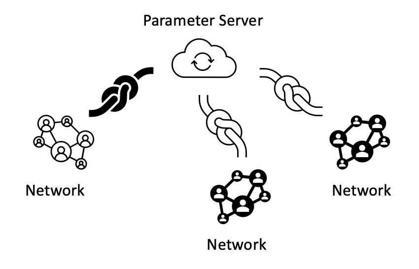
Figure 1: The System Architecture of Hierarchical Learning

The information exchange across networks is expensive and should occur only once in a while. To incorporate robustness, we focus on the challenging communication failures wherein a communication link may drop the transmitted messages unexpectedly and without notifying the sender. We do not impose any statistical patterns on the link failures; instead, we only require a link to function properly at least once during a time window. To the best of our knowledge, no existing relevant work considered such strong link failures.

We propose two hierarchical “consensus + innovation” algorithms for the state estimation and tracking problems, respectively. Under our algorithms, the parameter server does simple averaging over a small subset of agents. The state estimation problem can be viewed as a special case of the tracking problem. Nevertheless, in this paper, we study the state estimation and the general tracking problems separately; our results of the state estimation problem gives a better convergence rate. In both of these algorithms, we use a novel hierarchical push-sum consensus component wherein for each subnetwork only a designated agent needs to exchange messages with the parameter server and such exchange only occurs once in a while. For the state estimation, we use dual averaging as the local innovation component. State tracking is much harder to tackle in the presence of dropping-link failures and the standard integration of the consensus and dual averaging is no longer feasible. Our algorithm introduces a pair of additional variables per link and ensure the relevant local variables evolve according to the state dynamics, and use projected local gradient descent as the local innovation component. We also characterize the convergence rates of both of the algorithms under linear local observation model and minimal technical assumptions. Finally, we provide simulation results to illustrate the robustness and communication efficiency of our method.

II Problem Formulation

II-A System Model

We consider a hierarchical system architecture in which the agents are clusters into $M$ sub-networks, and a parameter server (PS) exists to aid the information exchanges among sub-networks. Similar system architecture is adopted in the literature [12, 20, 11]. The connection among each multi-agent network $S_{i}$ is time-varying and is formally represented by graphs $G({\mathcal{V}}_{i},{\mathcal{E}}_{i}[t])$, where ${\mathcal{V}}_{i}=\{v^{i}_{1},\cdots,v^{i}_{n_{i}}\}$ is node set and ${\mathcal{E}}_{i}[t]$ is the set of all directed edges. Specifically, there exists ${\mathcal{E}}_{i}$ such that ${\mathcal{E}}_{i}[t]\subseteq{\mathcal{E}}_{i}$ for each $t$. Let $N:=\sum_{i=1}^{M}n_{i}$. Agents in the same sub-network can exchange messages subject to the given communication network $G({\mathcal{V}}_{i},{\mathcal{E}}_{i}[t])$ at time $t$. No messages can be exchanged directly between agents in different sub-networks. In addition, the PS has the freedom in querying and pushing messages to any agent. Nevertheless, such message exchange is costly and needs to be sparse.

For an arbitrary agent $j$ in network $S_{i}$, let ${\mathcal{I}}_{j}^{i}[t]=\{k\mid(k,j)\in{\mathcal{E}}_{i}[t]\}$ and ${\mathcal{O}}_{j}^{i}[t]=\{k\mid(j,k)\in{\mathcal{E}}_{i}[t]\}$, respectively, be the sets incoming and outgoing neighbors to agent $j$. For notational convenience, we denote $d_{j}^{i}[t]=\left|O_{j}^{i}[t]\right|$.

Throughout this paper, we use the terminology “node” and “agent” interchangeably.

II-B Threat Model

We follow the network fault model adopted in [15] to consider packet-dropping link failures. Specifically, any communication link may unexpectedly drop a packet transmitted through it, and the sender is unaware of such packet lost. If a link successfully delivers messages at communication round $t$, we say this link is operational at round $t$.

Assumption 1

We assume that a link in ${\mathcal{E}}_{i}$ is operational at least once every $B$ communication round, for some positive constant $B$ for each $i=1,\cdots,M$.

Remark 1

As observed in [18, 13, 15], the above threat model is much harder to tackle compared with the ones wherein each agent is aware of the message delivery status. Though knowing real-time knowledge of out-going degree is reasonable, in harsh and versatile deployment environments such as undersea, the communication channels between two neighboring entities may suffer strong interference, leading to rapidly changing channel conditions and, consequently, unsuccessful message delivery.

II-C State Dynamics and Local Observation Models

State dynamics

Each of the agent is interested in learning the $d$-dimensional state of a moving target $w^{*}[t]$ that follows the dynamics

$$w^{*}[t]=Aw^{*}[t-1]~{}~{}~{}\forall~{}t\geq 1,$$ (1)

where $A\in{\mathbb{R}}^{d\times d}$ is known to each agent, and $w^{*}[t]\in{\mathcal{W}}\subseteq{\mathbb{R}}^{d}$. For example, each autonomous vehicle needs to keep track of neighboring vehicles, where the global state contains the statuses of the spatial position, the velocity, and the acceleration of the target. Clearly, the state dynamic is approximately a known linear matrix.

An interesting special case of Eq.(1) is when $A=I$, under which the target state is time-invariant, i.e., $w^{*}[t]=w^{*}[0]$ for all $t$. This special case is often referred to as the state estimation problem [2].

Local observation

In every iteration $t$, each agent locally takes measurements of the underlying truth $w^{*}[t]$. We focus on the a linear observation model which is commonly adopted in literature [16, 9, 14]: For a specific agent $j\in{\mathcal{V}}_{i}$ at time $t$:

$$y_{j}^{i}[t]:=H^{i}_{j}w^{*}[t]+\xi_{j}^{i}[t]$$ (2)

where $H_{j}^{i}$ is the local observation matrix, and $\xi^{i}_{j}[t]$ is the observation noise. We assume that the observation noise $\xi^{i}_{j}[t]$ is independent across time $t$ and across agents $j$. In addition, $\mathbb{E}\left[(\xi^{i}_{j}[t])^{\top}\xi^{i}_{j}[t]\right]\leq\sigma^{i}_{j}$. In practice, the observation matrix $H^{i}_{j}$ is often fat. Thus, to correctly estimate/track $w^{*}[t]$, agents must collaborate with others.

III Hierarchical Average Consensus in the Presence of Packet-dropping Failures

We introduce an average consensus algorithm (Algorithm 1), which extends our prior work [15] to the hierarchical system architecture. The algorithm in [15] can be viewed as a variant of that in [17], wherein finite-time convergence is not guaranteed and the corresponding rates are missing.

Up to line 13 in Algorithm 1 is the parallel execution of the fast robust push-sum [15] over the $M$ subnetworks. Lines 14-23 describe the novel information fusion cross the subnetworks, which only occurs once every $\Gamma$ iterations.

1 Initialization: For each sub-network $i=1,\cdots,M$: $z_{j}^{i}[0]=w_{j}^{i}\in{\mathbb{R}}^{d}$, $m^{i}_{j}[0]=1\in{\mathbb{R}},$ $\sigma_{j}^{i}[0]={\bf 0}\in{\mathbb{R}}^{d}$, $\widetilde{\sigma}_{j}^{i}[0]=0\in{\mathbb{R}}$, and $\rho^{i}_{j^{\prime}j}[0]={\bf 0}\in{\mathbb{R}}^{d}$, $\widetilde{\rho}^{i}_{j^{\prime}j}[0]=0\in{\mathbb{R}}$ for each incoming link, i.e., $j^{\prime}\in{\mathcal{I}}_{j}^{i}$.

2In parallel, each agent in parallel does:

3 for $t\geq 1$ do

4       $\sigma_{j}^{i+}[t]\leftarrow\sigma_{j}^{i}[t-1]+\frac{z_{j}^{i}[t-1]}{d_{j}^{i}[t]+1}$, $\widetilde{\sigma}_{j}^{i+}[t]\leftarrow\widetilde{\sigma}_{j}^{i}[t-1]+\frac{m_{j}^{i}[t-1]}{d_{j}^{i}[t]+1}$;

5      

6      Broadcast $\left(\sigma^{i+}_{j}[t],\widetilde{\sigma}^{i+}_{j}[t]\right)$ to outgoing neighbors;

7      

8      for each incoming link $(j^{\prime},j)\in{\mathcal{E}}_{i}[t]$ do

9            if message $\left(\sigma^{i+}_{j^{\prime}}[t],\widetilde{\sigma}^{i+}_{j^{\prime}}[t]\right)$ is received then

10                  $\rho^{i}_{j^{\prime}j}[t]\leftarrow\sigma^{i+}_{j^{\prime}}[t]$,    $\widetilde{\rho}^{i}_{j^{\prime}j}[t]\leftarrow\widetilde{\sigma}^{i+}_{j^{\prime}}[t]$;

11            else

12                   $\rho^{i}_{j^{\prime}j}[t]\leftarrow\rho^{i}_{j^{\prime}j}[t-1]$,   $\widetilde{\rho}^{i}_{j^{\prime}j}[t]\leftarrow\widetilde{\rho}^{i}_{j^{\prime}j}[t-1]$;

13            

14      $z_{j}^{i+}[t]\leftarrow\frac{z_{j}^{i}[t-1]}{d_{j}^{i}[t]+1}+\sum_{j^{\prime}\in{\mathcal{I}}_{j}^{i}[t]}\left(\rho^{i}_{j^{\prime}j}[t]-\rho^{i}_{j^{\prime}j}[t-1]\right)$;

15      

16      $m_{j}^{i+}[t]\leftarrow\frac{m_{j}^{i}[t-1]}{d_{j}^{i}[t]+1}+\sum_{j^{\prime}\in{\mathcal{I}}_{j}^{i}[t]}(\widetilde{\rho}^{i}_{j^{\prime}j}[t]-\widetilde{\rho}^{i}_{j^{\prime}j}[t-1])$.

17      $\sigma^{i}_{j}[t]\leftarrow\sigma^{i+}_{j}[t]+\frac{z_{j}^{i+}[t]}{d_{j}^{i}[t]+1}$, $\widetilde{\sigma}^{i}_{j}[t]\leftarrow\widetilde{\sigma}^{i+}_{j}[t]+\frac{m_{j}^{i+}[t]}{d_{j}^{i}[t]+1}$, $z_{j}^{i}[t]\leftarrow\frac{z_{j}^{i+}[t]}{d_{j}^{i}[t]+1}$, $m_{j}^{i}[t]\leftarrow\frac{m_{j}^{i+}[t]}{d_{j}^{i}[t]+1}$;

18      

19

20if $j$ is a designated agent of network $S_{i}$ then

21       if $t\mod\Gamma=0$ then

22             Send $\frac{1}{2}z_{j}^{i}[t]$ and $\frac{1}{2}m_{j}^{i}[t]$ to the PS;

23            

24            Upon receiving messages from the PS do

25             update $z_{j}^{i}[t]\leftarrow\frac{1}{2}z_{j}^{i}[t]+\frac{1}{2M}\sum_{i=1}^{M}z_{i_{0}}^{i}[t]$;

26             $m_{j}^{i}[t]\leftarrow\frac{1}{2}m_{j}^{i}[t]+\frac{1}{2M}\sum_{i=1}^{M}m_{i_{0}}^{i}[t]$;

27            

28      

29

30if $t\mod\Gamma=0$ then

31       The PS does the following:

32      Wait to receive $z_{i_{0}}^{i}[t]$ and $m_{i_{0}}^{i}[t]$ from each designated agent of the $M$ networks;

33      

34      Compute and send $\frac{1}{M}\sum_{i=1}^{M}\frac{1}{2}z_{i_{0}}^{i}[t]$ and $\frac{1}{M}\sum_{i=1}^{M}\frac{1}{2}m_{i_{0}}^{i}[t]$ to all designated agents $i_{0}$ for $i=1,\cdots,M$.

35

Algorithm 1 Hierarchical Push-Sum (HPS)

Similar to the standard Push-Sum [10], in addition to the primary variable $z_{j}^{i}$, each agent $j$ keeps a mass variable $m_{j}^{i}$ to correct the possible bias caused by the graph structure, and uses the ratio $z_{j}^{i}/m_{j}^{i}$ to estimate the average consensus. The correctness of push-sum relies crucially on mass preservation (i.e., $\sum_{i=1}^{M}\sum_{j=1}^{n_{i}}m_{j}^{i}[t]=N$) holds for all $t$. The variables $\sigma$, $\widetilde{\sigma}$, $\rho$, and $\widetilde{\rho}$ are introduced to recover the dropped messages. Specifically, $\sigma_{j}^{i}[t]$ and $\widetilde{\sigma}_{j}^{i}[t]$ are used to record how much value and mass that agent $j$ (in subnetwork $i$) have been sent to each of the outgoing neighbor of agent $j$ up to time $t$. Corresponding, $\rho^{i}_{j^{\prime}j}[t]$ and $\widetilde{\rho}^{i}_{j^{\prime}j}[t]$ are used to record how much value and mass have been received by agent $j$ through the link $(j^{\prime}j)\in{\mathcal{E}}_{i}$. On the technical side, we use augmented graphs (detailed in Definition 1 of Appendix A) to show convergence. To control the trajectory smoothness of the $z_{j}^{i}/m_{j}^{i}$ (at both normal agents and virtual agents), in each iteration, both $z$ and $m$ are updated twice in lines 11 to 13.

For each network, we choose an arbitrary agent as the network representative, and only this designated agent can exchange messages with the PS. Let $i_{0}$ denote the designated agent of network $i$. Every other $\Gamma$ iterations, each designated agent pushes 1/2 of its local value and mass to the PS. The PS computes the received average value and mass, and sends the averages back to each designated agent. Each designated agent then updates its local value and mass as ones pushed back from the PS.

Assumption 2

Each network $({\mathcal{V}}_{i},{\mathcal{E}}_{i})$ is strongly connected for $i=1,\cdots,M$.

Denote the diameter of $G({\mathcal{V}}_{i},{\mathcal{E}}_{i})$ as $D_{i}$. Let $D^{*}:=\max_{i\in[M]}D_{i}$. Let $\beta_{i}=\frac{1}{\max_{j\in{\mathcal{V}}_{i}}(d_{j}^{i}+1)^{2}}$.

Theorem 1

Choose $\Gamma=BD^{*}$. Suppose that Assumptions 1 and 2 hold, and that $t\geq 2\Gamma$. Then

$$\left\|{\frac{z_{j}^{i}[t]}{m_{j}^{i}[t]}-\frac{1}{N}\sum_{i=1}^{M}\sum_{j=1}^{n_{i}}w_{j}^{i}}\right\|_{2} \leq\frac{4M^{2}\sum_{i=1}^{M}\sum_{j=1}^{n_{i}}\left\|{w_{j}^{i}}\right\|_{2}\gamma^{\lfloor\frac{t}{2\Gamma}\rfloor-1}}{\left(\min_{i\in[M]}\beta_{i}\right)^{2D^{*}B}N},$$

where $\gamma=1-\frac{1}{4M^{2}}\left(\min_{i\in[M]}\beta_{i}\right)^{2D^{*}B}$.

Henceforth, for ease of exposition, we adopt the simplification that $\lfloor t/2\Gamma\rfloor-\lceil r/2\Gamma\rceil=(t-r)/2\Gamma.$ Such simplification does not affect the order of convergence rate. Exact expression can be recovered while a straightforward bookkeeping of the floor and ceiling in the calculation.

Theorem 1 says that, despite packet-dropping link failures and sparse communication between the networks and the PS, the consensus error $\left\|{\frac{z_{j}^{i}[t]}{m_{j}^{i}[t]}-\frac{1}{N}\sum_{i=1}^{M}\sum_{j=1}^{n_{i}}w_{j}^{i}}\right\|_{2}$ decays to 0 exponentially fast. Clearly, the more reliable the network (i.e. smaller $B$) and the more frequent across networks information fusion (i.e. smaller $\Gamma$), the faster the convergence rate.

Remark 2

Partitioning the agents into $M$ subnetworks immediately leads to smaller network diameters $D^{*}$. Hence, compared with a gigantic single network, the term $\left(\min_{i\in[M]}\beta_{i}\right)^{2D^{*}B}$ for the $M$ sub-networks is significantly larger, i.e., faster convergence.

Remark 3

It turns out that our bound in Theorem 1 is loose in quantifying the total number of global communication. Specifically, for any given $\epsilon>0$, to reduce the error to $O(\epsilon)$, based on the bound in Theorem 1, it takes $t\geq\Omega\left(\Gamma\log\epsilon/\log\gamma\right)$, i.e., larger $\Gamma$ leads to slower convergence to $O(\epsilon)$. However, our preliminary simulation results (presented in Fig. 3) indicate that if the cost of global communication is significant enough, then a larger $\Gamma$ may converges faster in terms of total communication delay.

IV State Estimation

In this section, we study the special case of Eq.(1) when $A=I$, i.e., the state estimation problem. We use a “consensus” + “innovation” approach with Algorithm 1 as the consensus component and use dual averaging as the innovation component. Specifically, we add the following lines of pseudo code right after line 12 inside the outer for-loop in Algorithm 1 – at the end of the for-loop: Obtain observation $y_{j}^{i}[t]$;
Compute a stochastic gradient $g_{j}^{i}[t]$ of $f_{j}^{i}$;
$z_{j}^{i}[t]\leftarrow z_{j}^{i}[t-1]+g_{j}^{i}[t]$;
$w_{j}^{i}[t]\leftarrow\prod_{w\in{\mathcal{W}}}^{\varphi}(\frac{z^{i}_{j}[t]}{m^{i}_{j}[t]},\eta[t-1])$. Next we explain the added pseudo code.

(I) Each agent $j$ first obtains a new observation $y_{i}[t]$ according to Eq. (2).

(II) For ease of exposition, the local function $f_{j}^{i}$ at agent $j$ of network $S_{i}$ is defined as:

$$f^{i}_{j}(w):=\frac{1}{2}\mathbb{E}[\|H^{i}_{j}w-y^{i}_{j}\|_{2}^{2}],$$ (3)

where $w\in{\mathcal{W}}$. Let $F$ denote the global objective, i.e.,

$$f:=\sum_{i=1}^{M}\sum_{j=1}^{n_{i}}f^{i}_{j}.$$ (4)

Despite the fact $f_{j}^{i}$ is well-defined, it is unknown to agent $j$. This is because the observation noise $\xi_{j}^{i}$ distribution is unknown and agent $j$ cannot evaluate the expectation in (3). Hence, we cannot perform the standard distributed dual averaging. Fortunately, as $H_{j}^{i}$ is known, agent $j$ can access the natural stochastic gradient of (3)

$$g^{i}_{j}[t]=H_{j}^{\top}\left(H_{j}w[t-1]-y^{i}_{j}[t-1]\right).$$ (5)

We calculate $g^{i}_{j}[t]$ with $y^{i}_{j}[t-1]$ instead of $y^{i}_{j}[t]$ is for ease of exposition in the analysis. We can replace $y^{i}_{j}[t-1]$ with $y^{i}_{j}[t]$, the analysis remains the same except for time index changes.

(III) The variable $z_{j}^{i}[t]$ is used to cumulative all the locally computed stochastic gradients up to time $t$.

(IV) The update of the local estimate $w_{j}^{i}$ uses the function $\prod_{w\in{\mathcal{W}}}^{\varphi}\left(z,\eta\right):=\arg\min_{w\in{\mathcal{W}}}\left\{\left\langle z,w\right\rangle+\frac{1}{\eta}\varphi(w)\right\}$, where $\eta>0$ is the stepsize, and $\varphi:{\mathbb{R}}^{d}\to{\mathbb{R}}$ is a non-negative and $1$-strongly convex function with respect to $\ell_{2}$ norm, i.e., $\varphi(w^{\prime})\geq\varphi(w)+\left\langle\nabla\varphi(w),w^{\prime}-w\right\rangle+\frac{1}{2}\left\|{w^{\prime}-w}\right\|_{2}$.

One example of such $1$-strongly convex function is the $\ell_{2}$ norm, i.e., $\varphi(w)=\frac{1}{2}\left\|{w}\right\|_{2}^{2}$. We will choose a sequence of delaying stepsizes $\{\eta[t]\}_{t=0}^{\infty}$, which will be specified in Theorem 2.

Assumption 3

The constraint set ${\mathcal{W}}$ is compact.

Assumption 4

Let $K\triangleq\sum_{i=1}^{M}\sum_{j=1}^{n_{i}}\left((H_{j}^{i})^{\top}H_{j}^{i}\right)$. The matrix $K$ is positive definite.

Notably, Assumption 4 is necessary even for the single network and failure-free setting.

Denote the diameter of set ${\mathcal{W}}$ as

$$R_{0}:=\max_{w,w^{\prime}\in{\mathcal{W}}}\left\|{w-w^{\prime}}\right\|_{2}$$ (6)

Proposition 1

Suppose that Assumption 3 holds. Then $f$ is $L$-Lipschitz continuous with $L:=R_{0}\left\|{K}\right\|_{2}$, i.e., $\left\|{f(w)-f(w^{\prime})}\right\|_{2}\leq L\left\|{w-w^{\prime}}\right\|_{2}$ for all $w,w^{\prime}\in{\mathcal{W}}.$ Moreover, $f_{j}^{i}$ is also $L$-Lipschitz continuous $\forall i\in[M],j\in{\mathcal{V}}_{i}$.

Assumption 5

The observation noise $\xi_{j}^{i}[t]$ is independent across time $t$ and across agents $j\in{\mathcal{V}}_{i}$ for $i=1,\cdots,M$. Moreover, $\left\|{H_{ij}^{\top}\xi_{j}^{i}}\right\|_{2}\leq B_{0}$ for all agents.

Under Assumptions 3 and 5, the following proposition holds immediately.

Proposition 2

Suppose that Assumptions 3 and 5 hold. Let $L_{0}:=2R_{0}\left\|{K}\right\|_{2}+B_{0}$. It is true that $\left\|{g_{j}^{i}(w)}\right\|_{2}\leq L_{0}$.

For each agent, we define $\widehat{w}_{j}^{i}[t]:=\frac{1}{t}\sum_{r=1}^{t}w_{j}^{i}[r]$ to be the running average $w_{j}^{i}[t]$.

Theorem 2

Suppose that Assumptions 1-4 hold, and that $\varphi(w^{*})\leq R^{2}$. Let $\left\{\eta[t]\right\}_{t=0}^{\infty}$ be a sequence of non-increasing step sizes. For any $\delta\in(0,1)$, the following holds with probability at least $(1-\delta)$:

$$\left\|{\widehat{w}_{j}^{i}[T]-w^{*}}\right\|_{2}^{2}\leq\frac{1}{\lambda_{\min}}\left(\frac{NL_{0}^{2}}{2T}\sum_{t=1}^{T}\eta[t-1]+\frac{NR^{2}}{T\eta[T]}\right.$$

$$+\left.\frac{4M^{2}L_{0}^{2}\gamma^{\frac{1}{2\Gamma}}}{\left(1-\gamma^{\frac{1}{2\Gamma}}\right)\left(\min_{i\in[M]}\beta_{i}\right)^{2D^{*}B}}\frac{1}{T}\sum_{t=1}^{T}\eta[t-1]\right.$$

$$\qquad\qquad\qquad\qquad\qquad\qquad\qquad\left.+4NLR\sqrt{\frac{\log\frac{1}{\delta}}{T}}.\right)$$

where $\lambda_{\min}$ is the smallest eigenvalue of $K$.

Remark 4

Choosing $\eta[t]=\frac{1}{\sqrt{t}}$, it becomes

$$\left\|{\widehat{w}_{j}^{i}[T]-w^{*}}\right\|_{2}^{2}\leq\frac{1}{\lambda_{\min}}\left(\frac{NL_{0}^{2}}{2\sqrt{T}}+\frac{N}{\sqrt{T}}R^{2}\right.$$

$$+\left.\frac{4M^{2}L_{0}^{2}\gamma^{\frac{1}{2\Gamma}}}{\left(1-\gamma^{\frac{1}{2\Gamma}}\right)\left(\min_{i\in[M]}\beta_{i}\right)^{2D^{*}B}}\frac{1}{\sqrt{T}}+4NLR\sqrt{\frac{\log\frac{1}{\delta}}{T}}.\right)$$

V State Tracking

In the state tracking problem, the agents try to collaboratively track $w^{*}[t]$. We present the full description of our algorithm in Algorithm 2. Our algorithm uses projected gradient descent as the local innovation component.

In each round, in line 4, each agent gets a new observation $y_{j}^{i}[t]$. However, the local stochastic gradient is computed on the measurement obtained in the previous round $t-1$. As can be seen from our analysis, we use such one step setback to align the impacts of the global dynamics $A$ with the relevant parameters evolution. In addition, in line 18, we apply $A$ to local $z$ sequence update. Recall that if a link does not function properly, the sent value and mass are stored in virtual nodes (the nodes that correspond to the edges). Hence, we apply $A$ to the auxiliary variables $\sigma$ and $\rho$ as well. Specifically, we update $\rho_{j^{\prime}j}^{i}$ and $\widetilde{\rho}_{j^{\prime}j}^{i}$ twice – the first time in lines 9-12, and the second time in lines 16 and 17. In line 15, we apply $A$ to the original update of $\sigma$. Notably, we apply $A$ to $z$ and auxiliary variables that are relevant to $z$ only; we do not apply $A$ to the mass update. In line 19, $\prod_{{\mathcal{W}}}[\cdot]$ is an operator that projects any given $w\in{\mathbb{R}}^{d}$ onto ${\mathcal{W}}$. This projection is used to ensure boundedness of stochastic gradients.

1 Initialization: For each sub-network $i=1,\cdots,M$: $z_{j}^{i}[0]=w_{j}^{i}\in{\mathbb{R}}^{d}$, $m^{i}_{j}[0]=1\in{\mathbb{R}},$ $\sigma_{j}^{i}[0]={\bf 0}\in{\mathbb{R}}^{d}$, $\widetilde{\sigma}_{j}^{i}[0]=0\in{\mathbb{R}}$, and $\rho^{i}_{j^{\prime}j}[0]={\bf 0}\in{\mathbb{R}}^{d}$, $\widetilde{\rho}^{i}_{j^{\prime}j}[0]=0\in{\mathbb{R}}$ for each incoming link, i.e., $j^{\prime}\in{\mathcal{I}}_{j}^{i}$.

2In parallel, each agent in parallel does:

3 for $t\geq 1$ do

4       Obtain measurement $y^{i}_{j}[t]$;

5       Compute a local stochastic gradient $g^{i}_{j}[t]$ that corresponds to the previous measurement $y^{i}_{j}[t-1]$ evaluated at local estimated $w^{i}_{j}[t-1]$;

6      

7      $\sigma_{j}^{i+}[t]\leftarrow\sigma_{j}^{i}[t-1]+\frac{z_{j}^{i}[t-1]}{d_{j}^{i}[t]+1}$, $\widetilde{\sigma}_{j}^{i+}[t]\leftarrow\widetilde{\sigma}_{j}^{i}[t-1]+\frac{m_{j}^{i}[t-1]}{d_{j}^{i}[t]+1}$;

8      

9      Broadcast $\left(\sigma^{i+}_{j}[t],\widetilde{\sigma}^{i+}_{j}[t]\right)$ to outgoing neighbors;

10      

11      for each incoming link $(j^{\prime},j)\in{\mathcal{E}}_{i}[t]$ do

12            if message $\left(\sigma^{i+}_{j^{\prime}}[t],\widetilde{\sigma}^{i+}_{j^{\prime}}[t]\right)$ is received then

13                  $\rho^{i+}_{j^{\prime}j}[t]\leftarrow\sigma^{i+}_{j^{\prime}}[t]$,    $\widetilde{\rho}^{i+}_{j^{\prime}j}[t]\leftarrow\widetilde{\sigma}^{i+}_{j^{\prime}}[t]$;

14            else

15                   $\rho^{i+}_{j^{\prime}j}[t]\leftarrow\rho^{i}_{j^{\prime}j}[t-1]$,   $\widetilde{\rho}^{i+}_{j^{\prime}j}[t]\leftarrow\widetilde{\rho}^{i}_{j^{\prime}j}[t-1]$;

16            

17      $z_{j}^{i+}[t]\leftarrow\frac{z_{j}^{i}[t-1]}{d_{j}^{i}[t]+1}+\sum_{j^{\prime}\in{\mathcal{I}}_{j}^{i}[t]}\left(\rho^{i}_{j^{\prime}j}[t]-\rho^{i}_{j^{\prime}j}[t-1]\right)$;

18      

19      $m_{j}^{i+}[t]\leftarrow\frac{m_{j}^{i}[t-1]}{d_{j}^{i}[t]+1}+\sum_{j^{\prime}\in{\mathcal{I}}_{j}^{i}[t]}(\widetilde{\rho}^{i}_{j^{\prime}j}[t]-\widetilde{\rho}^{i}_{j^{\prime}j}[t-1])$;

20      

21      $\sigma^{i}_{j}[t]\leftarrow A(\sigma^{i+}_{j}[t]+\frac{z_{j}^{i+}[t]}{d_{j}^{i}[t]+1})$, $\widetilde{\sigma}^{i}_{j}[t]\leftarrow\widetilde{\sigma}^{i+}_{j}[t]+\frac{m_{j}^{i+}[t]}{d_{j}^{i}[t]+1}$;

22      

23      for each incoming link $(j^{\prime},j)\in{\mathcal{E}}_{i}[t]$ do

24             $\rho_{j^{\prime}j}^{i}[t]\leftarrow A\rho_{j^{\prime}j}^{i+}[t]$, and $\widetilde{\rho}_{j^{\prime}j}^{i}[t]\leftarrow\widetilde{\rho}_{j^{\prime}j}^{i+}[t]$.

25      

26      $z_{j}[t]\leftarrow A\frac{z_{j}^{+}[t]}{d_{j}[t]+1}-\eta[t]g_{j}[t]$, and $m_{j}[t]\leftarrow\frac{m_{j}^{+}[t]}{d_{j}[t]+1}$;

27       $w_{j}[t]=\prod_{{\mathcal{W}}}\left[\frac{z_{j}[t]}{m_{j}[t]}\right]$.

28

29if $j$ is a designated agent of network $S_{i}$ then

30       if $t\mod\Gamma=0$ then

31             Send $\frac{1}{2}z_{j}^{i}[t]$ and $\frac{1}{2}m_{j}^{i}[t]$ to the PS;

32            

33            Upon receiving messages from the PS do

34             update $z_{j}^{i}[t]\leftarrow\frac{1}{2}z_{j}^{i}[t]+\frac{1}{2M}\sum_{i=1}^{M}z_{i_{0}}^{i}[t]$;

35             $m_{j}^{i}[t]\leftarrow\frac{1}{2}m_{j}^{i}[t]+\frac{1}{2M}\sum_{i=1}^{M}m_{i_{0}}^{i}[t]$;

36            

37      

38

39if $t\mod\Gamma=0$ then

40       The PS does the following:

41      Wait to receive $z_{i_{0}}^{i}[t]$ and $m_{i_{0}}^{i}[t]$ from each designated agent of the $M$ networks;

42      

43      Compute and send $\frac{1}{M}\sum_{i=1}^{M}\frac{1}{2}z_{i_{0}}^{i}[t]$ and $\frac{1}{M}\sum_{i=1}^{M}\frac{1}{2}m_{i_{0}}^{i}[t]$ to all designated agents $i_{0}$ for $i=1,\cdots,M$.

44

Algorithm 2 Collaborative Tracking Algorithm

In addition to the aforementioned assumptions, the following assumptions will be used in our analysis.

Assumption 6

The global linear dynamic matrix $A$ is positive semi-definite with $\left\|{A}\right\|_{2}\leq 1$.

Notably, $\left\|{\bm{I}}\right\|_{2}=1$, satisfying Assumption 6.

Assumption 7

The set ${\mathcal{W}}$ contains $w^{*}[t]$ for all $t$.

We define $\bar{z}=-\frac{1}{N}\sum_{i=1}^{M}\sum_{j=1}^{n_{i}}z_{j}^{i}[t]$, which differs from standard aggregation by a “-” sign.

Theorem 3

Suppose that Assumptions 1-5 hold. Choose $\eta[t]=\frac{1}{\lambda_{1}t}$ for $t\geq 1$, and $\eta[0]=\frac{1}{\lambda_{1}}$. Suppose that Assumption 6 holds. Let $b=\left\|{A}\right\|_{2}\gamma^{\frac{1}{\Gamma}}$. Let $t_{0}=\frac{2}{\log 1/b}\log\left(\frac{2}{\log 1/b}\right)$. Then

$$\left\|{w_{j}^{i}[t]-\bar{z}[t]}\right\|_{2}\leq\begin{cases}\frac{16M^{2}L_{0}}{\left(\min_{i\in[M]}\beta_{i}\right)^{2D^{*}B}\lambda_{1}(1-b)t},~{}~{}&\text{if }~{}t\geq t_{0}\\ \frac{4M^{2}L_{0}t_{0}}{\left(\min_{i\in[M]}\beta_{i}\right)^{2D^{*}B}\lambda_{1}},~{}~{}&\text{if }~{}t<t_{0}\end{cases}$$ (7)

Moreover, when $T\geq t_{0}$, for any given $\delta\in(0,1)$, the following holds with probability at least $(1-\delta)$:

$$\left\|{w^{i}_{j}[T]-w^{*}[t]}\right\|_{2}\leq\left\|{w_{0}^{*}}\right\|_{2}\exp\left(\frac{\lambda_{1}}{\lambda_{d}}\right)\frac{1}{T}$$

$$\qquad+\frac{\exp\left(\lambda_{1}/\lambda_{d}\right)4M^{2}L_{0}t^{2}_{0}}{\left(\min_{i\in[M]}\beta_{i}\right)^{2D^{*}B}\lambda_{1}}\frac{1}{T}$$

$$\qquad+\frac{32M^{2}L_{0}\exp\left(\lambda_{1}/\lambda_{d}\right)}{\left(\min_{i\in[M]}\beta_{i}\right)^{2D^{*}B}\lambda_{1}(1-b)}\frac{\log(T+1)}{T}$$

$$\qquad+\frac{2B_{0}\exp\left(\lambda_{1}/\lambda_{d}\right)}{\lambda_{1}}\sqrt{\frac{d}{2t}\log(d/\delta)},$$ (8)

where $\lambda_{1}\geq\cdots\geq\lambda_{d}>0$ are the eigenvalues of $K$.

Proofs can be found in Appendix C.

Remark 5

For sufficiently large $T$, the dominance term in the upper bound of Eq.(3) is $\sqrt{\frac{d}{2T}\log(d/\delta)}B_{0}\log T$, which arises from the observation noise.

VI Numerical Results

To better illustrate the benefits of our method, we present simulated results below. We consider a 16-node network with a single parameter server node as shown in figure 2. We model the communication delay between a pair of nodes as a Poisson random variable. Communication within each of the three network clusters is inexpensive, with a cost $\lambda=\lambda_{local}$. Communication between any individual agent and the parameter server (node 0) is more expensive, with a cost $\lambda=c\lambda_{local}$. For our experiments we select $c=2$, that is to say the expected delay in communication is twice as long with the parameter server as it is for local communications.

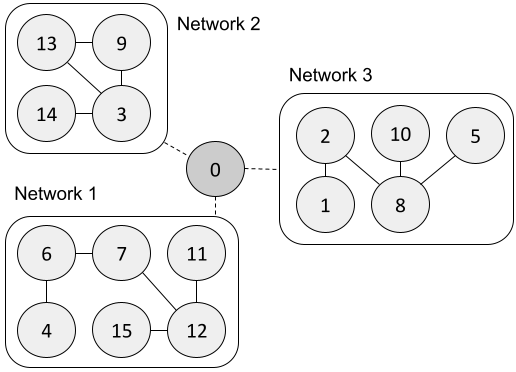
Figure 2: Simulated Network Structure.

We consider two separate observation models for state estimation and tracking, respectively. For state estimation, our ground truth state is a drawn from a 12-dimensional zero-mean Gaussian with identity covariance. For tracking, we similarly use a 2-dimensional Gaussian vector representing the X and Y coordinates of a moving object, having global dynamics $A=aI$, with $a=0.99$. Each agent has an identity observation matrix and i.i.d. Gaussian noise with variance 0.2 added to each dimension of the observation. We use a step size of 0.1 for all experiments.

In figure 3, we plot the average state estimation L2 error over time for various drop-link conditions $B$ and hierarchical synchronization frequency $\Gamma$. Observe first that our algorithm converges similarly with and without the addition of the noise introduced by dropped links ($B>1$). Second, the hierarchical decomposition ($\Gamma>1$) significantly speeds up the convergence compared to a “Full Graph” structure ($\Gamma$ = 1), as we avoid the expensive synchronization delay with the parameter server.

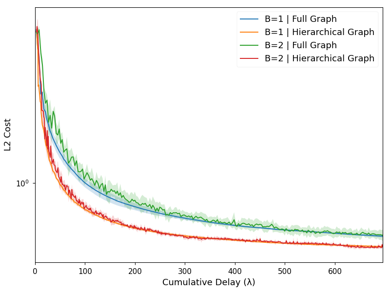
Figure 3: Graph of Cost for Varying Network and System Configurations.

For state tracking, we plot the average state estimate across agents within each sub-network over time in figure 4, where darker points indicate more recent positions in time.

Figure 4: State Tracking Simulation.

Appendix A Hierarchical Consensus

A-A Matrix Construction

The analysis of Theorem 1 relies on the notion of augmented graphs and a compact matrix representation of the dynamics of $z$ and $m$ over those augmented graphs.

Definition 1 (Augmented Graph)

[17] Given a graph $G({\mathcal{V}},{\mathcal{E}})$, the augmented graph $G^{a}({\mathcal{V}}^{a},{\mathcal{E}}^{a})$ is constructed as:

1. ${\mathcal{V}}^{a}={\mathcal{V}}\cup{\mathcal{E}}$: $|{\mathcal{E}}|$ virtual agents are introduced, each of which represents a link in $G({\mathcal{V}},{\mathcal{E}})$. Let $n_{j^{\prime}j}$ be the virtual agent corresponding to edge $(j^{\prime},j)$.

2. ${\mathcal{E}}^{a}\triangleq{\mathcal{E}}\cup\left\{\left(j^{\prime},n_{j^{\prime}j}\right),(n_{j^{\prime}j},j),~{}\forall~{}(j^{\prime},j)\in{\mathcal{E}}\right\}$.

An example can be found in Fig. 5. In the original graph (left), the node and edge sets are ${\mathcal{V}}=\{1,2,3\}$ and ${\mathcal{E}}=\{(1,2),(2,1),(1,3),(3,2)\}$, respectively. The four green nodes in the corresponding augmented graph (right) are the virtual agents and the dashed arrows indicate the added links.

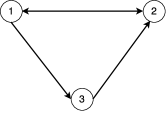
Figure 5: Augmented graph example

We study the information flow in the augmented graphs rather than in the original systems. When a message is not successfully delivered over a link, our Algorithm 1 uses a well-calibrated mechanism to recover such a message and to convert it into a delayed message. Intuitively, we can treat the delayed message as the ones that are first sent to virtual nodes, and then are held for at most $B-1$ iterations, and finally are released to the destination node. For each subnetwork $S_{i}$, let $m_{i}:=|{\mathcal{E}}_{i}|$ denote the number of edges. Let $\widetilde{N}:=\sum_{i=1}^{M}\left(n_{i}+m_{i}\right)$. Thus, we construct a matrix $\bm{M}[t]\in{\mathbb{R}}^{\widetilde{N}\times\widetilde{N}}$ as follows.

Non-global fusion iterations

Fix a network $S_{i}$. Fix $t$ be arbitrary iteration such that $t\mod\Gamma\not=0$. The matrix construction is the same as that in [15]. For completeness, we present the construction as follows.

For each link $(j,j^{\prime})\in{\mathcal{E}}_{i}[t]$, and $t\geq 1$, as

$${\mathsf{B}}^{i}_{(j,j^{\prime})}[t]\triangleq\left\{\begin{tabular}[]{ll}1, ~{} if $(j,j^{\prime})\in{\mathcal{E}}_{i}[t]$ and is reliable at time $t$;\\ 0, ~{} otherwise.\end{tabular}\right.$$ (11)

Recall that $z_{j}^{i}$ and $m_{j}^{i}$ are the value and mass for $j\in{\mathcal{V}}^{i}$. For each $(j,j^{\prime})\in{\mathcal{E}}_{i}[t]$,

$$z^{i}_{n_{j^{\prime}j}}[t]\triangleq\sigma^{i}_{j^{\prime}}[t]-\rho^{i}_{j^{\prime}j}[t],\quad m^{i}_{n_{j^{\prime}j}}[t]\triangleq\widetilde{\sigma}^{i}_{j^{\prime}}[t]-\widetilde{\rho}^{i}_{j^{\prime}j}[t],$$ (12)

with $z^{i}_{n_{j^{\prime}j}}[0]={\bf 0}\in{\mathbb{R}}^{d}$ and $m^{i}_{n_{j^{\prime}j}}[0]=0\in{\mathbb{R}}$. Intuitively, $z^{i}_{n_{j^{\prime}j}}[t]$ and $m^{i}_{n_{j^{\prime}j}}[t]$ are the value and weight that agent $j^{\prime}$ tries to send to agent $j$ not not successfully be delivered. Let

$${\bf M}_{j,j}[t]\triangleq\frac{1}{\left(d_{j}^{i}[t]+1\right)^{2}},$$

$${\bf M}_{j,j^{\prime}}[t]\triangleq\frac{{\mathsf{B}}^{i}_{(j^{\prime},j)}[t]}{\left(d_{j}^{i}[t]+1\right)\left(d_{j^{\prime}}^{i}[t]+1\right)},~{}\forall~{}j^{\prime}\in{\mathcal{I}}_{j}^{i}[t],$$

$${\bf M}_{j,n_{j^{\prime}j}}[t]\triangleq\frac{{\mathsf{B}}^{i}_{(j^{\prime},j)}[t]}{d_{j}^{i}[t]+1},~{}\forall~{}j^{\prime}\in{\mathcal{I}}^{i}_{j}[t],$$

$${\bf M}_{n_{j^{\prime}j},j^{\prime}}[t]\triangleq\frac{1}{\left(d_{j^{\prime}}^{i}[t]+1\right)^{2}}+\frac{1-{\mathsf{B}}^{i}_{(j^{\prime},j)}[t]}{d_{j^{\prime}}^{i}[t]+1},$$

$${\bf M}_{n_{j^{\prime}j},k}[t]=\frac{{\mathsf{B}}^{i}_{(k,j^{\prime})}[t]}{\left(d_{k}^{i}[t]+1\right)\left(d_{j^{\prime}}^{i}[t]+1\right)},~{}~{}~{}\forall~{}k\in{\mathcal{I}}^{i}_{j^{\prime}}[t],$$

$${\bf M}_{n_{j^{\prime}j},n_{kj^{\prime}}}[t]\triangleq\frac{{\mathsf{B}}^{i}_{(k,j^{\prime})}[t]}{d_{j^{\prime}}^{i}[t]+1},~{}~{}\forall~{}k\in{\mathcal{I}}^{i}_{j^{\prime}}[t];$$

$${\bf M}_{n_{j^{\prime}j}n_{j^{\prime}j}}[t]\triangleq 1-{\mathsf{B}}^{i}_{(j^{\prime},j)}[t].$$

and any other entry in ${\bf M}[t]$ be zero. It is easy to check that the obtained matrix ${\bf M}[t]$ is column stochastic, and that

$$\bm{z}[t]=\left(\bm{M}[t]\otimes\bm{I}\right)\bm{z}[t-1],~{}~{}~{}\forall~{}t\mod\Gamma\not=0,$$

where $\bm{z}[t]\in{\mathbb{R}}^{\widetilde{N}d}$ is the vector that stacks all the local $z$’s. The update of the weight vector has the same matrix form since the update of value $z$ and weight $m$ are identical.

Global fusion iterations

Fix $t$ be arbitrary iteration such that $t\mod\Gamma=0$. We construct matrix $\bm{M}$ in two steps. We let $\bar{\bm{M}}$ denote the matrix constructed the same way as above. Let $\bm{F}$ be the matrix that captures the mass push among the designated agents under the coordination of the parameter server. Specifically,

$$\bm{F}_{j_{0},j_{0}} =\frac{M+1}{2M}~{}~{}~{}~{}\text{for each designated agent }j_{0};$$

$$\bm{F}_{j_{0},j^{\prime}_{0}} =\frac{1}{2M}~{}~{}~{}~{}\text{for distinct designated agents }j_{0},j^{\prime}_{0},$$

with all the other entries being zeros. Henceforth, we refer to matrix $\bm{F}$ as hierarchical fusion matrix. Clearly, $\bm{F}$ is a doubly-stochastic matrix. Hence, we define $\bm{M}$ as

$$\bm{M}[t]=\bm{F}\bar{\bm{M}}[t].$$ (13)

It is easy to see that the dynamics of $\bm{z}[t]$ for $t\mod\Gamma=0$ also obey

$$\bm{z}[t]=\left(\bm{M}[t]\otimes\bm{I}\right)\bm{z}[t-1].$$

Overall

We have

$$\bm{z}[t] =\left(\bm{M}[t]\otimes\bm{I}\right)\left(\bm{M}[t-1]\otimes\bm{I}\right)\bm{z}[t-2]$$

$$=\left(\bm{M}[t]\otimes\bm{I}\right)\left(\bm{M}[t-1]\otimes\bm{I}\right)\cdots\left(\bm{M}[1]\otimes\bm{I}\right)\bm{z}[0].$$

That is, the evolution of $z$ is controlled by the matrix product $\bm{M}[t]\bm{M}[t-1]\cdots\bm{M}[1]$. In general, let ${\bf\Psi}(r,t)$ be the product of $t-r+1$ matrices

$${\bf\Psi}(r,t) \triangleq\prod_{\tau=r}^{t}\,{\bf M}^{\top}[\tau]={\bf M}^{\top}[r]{\bf M}^{\top}[r+1]\cdots{\bf M}^{\top}[t],$$

where $r\leq t$ with ${\bf\Psi}(t+1,t)\triangleq{\bf I}$ by convention, i.e., ${\bf\Psi}(r,t)=\left(\bm{M}[t]\bm{M}[t-1]\cdots\bm{M}[1]\right)^{\top}$. Notably, ${\bf M}^{\top}[\tau]$ is row-stochastic for each $\tau$ of interest. Without loss of generality, let us fix an arbitrary bijection between $\{N+1,\cdots,\widetilde{N}\}$ and $(j,j^{\prime})\in{\mathcal{E}}_{i}$ for $i=1,\cdots,M$. For $j\in{\mathcal{V}}_{i}$, we have

$$z_{j}^{i}[t] =\sum_{j^{\prime}=1}^{\widetilde{N}}z_{j^{\prime}}[0]{\bf\Psi}_{j^{\prime}j}(1,t)=\sum_{j^{\prime}=1}^{\widetilde{N}}w_{j^{\prime}}^{i}{\bf\Psi}_{j^{\prime}j}(1,t),$$ (14)

where the last equality holds due to $z_{j}[0]=w_{j}^{i}$ for $j=1,\cdots,N$ and $z_{j}[0]=0\in{\mathbb{R}}^{d}$ when $j>N$, i.e., when $j$ corresponds to an edge.

A-B Auxiliary Lemmas

To show the convergence of Algorithm 1, we investigate the convergence behavior of ${\bf\Psi}(r,t)$ (where $r\leq t$) using ergodic coefficients and some celebrated results obtained by Hajnal [7]. The remaining proof follows the same line as that in [18, 17], and is presented below for completeness.

Given a row stochastic matrix ${\bf A}$, coefficients of ergodicity $\delta({\bf A})$ is defined as:

$$\delta({\bf A}) \triangleq\max_{j}~{}\max_{i_{1},i_{2}}~{}\left|{\bf A}_{i_{1}j}-{\bf A}_{i_{2}j}\right|,$$ (15)

$$\lambda({\bf A}) \triangleq 1-\min_{i_{1},i_{2}}\sum_{j}\min\{{\bf A}_{i_{1}j},{\bf A}_{i_{2}j}\}.$$ (16)

Proposition 3

[7] For any $p$ square row stochastic matrices ${\bf Q}[1],{\bf Q}[2],\dots\bf Q[p]$, it holds that

$$\delta({\bf Q}[1]{\bf Q}[2]\ldots{\bf Q}[p])~{}\leq~{}\Pi_{k=1}^{p}~{}\lambda({\bf Q}[k]).$$ (17)

Proposition 3 implies that if $\lambda({\bf Q}[k])\leq 1-c$ for some $c>0$ and for all $1\leq k\leq p$, then $\delta({\bf Q}[1],{\bf Q}[2]\cdots{\bf Q}[p])$ goes to zero exponentially fast as $p$ increases. The following lemmas are useful in the analysis of our follow-up algorithms.

Lemma 1

For $r\leq t$ such that $\lfloor t/2\Gamma\rfloor-\lceil r/2\Gamma\rceil\geq 0$, it holds that $\delta\left({\bf\Psi}(r,t)\right)\leq\gamma^{(t-r)/2\Gamma},$ where $\gamma=1-\frac{1}{4M^{2}}\left(\min_{i\in[M]}\beta_{i}\right)^{2D^{*}B}$ as per Theorem 2.

Proof: The following rewriting holds:

$${\bf\Psi}(r,t) ={\bf\Psi}(r,\Gamma\lceil r/\Gamma\rceil)\left(\prod_{k=\lceil r/\Gamma\rceil}^{\lfloor t/\Gamma\rfloor-1}{\bf\Psi}(k\Gamma+1,(k+1)\Gamma)\right)$$

$$\qquad\qquad\qquad\qquad\qquad\times{\bf\Psi}(\Gamma\lfloor t/\Gamma\rfloor+1,\,t).$$

By Proposition 3, we have

$$\delta\left({\bf\Psi}(r,t)\right) \leq\prod_{k=\lceil r/2\Gamma\rceil}^{\lfloor t/2\Gamma\rfloor-1}\lambda\left({\bf\Psi}(2k\Gamma+1,2(k+1)\Gamma)\right)$$

$$\leq\gamma^{(t-r)/2\Gamma},$$

where $\gamma:=1-\frac{1}{4M^{2}}\left(\min_{i\in[M]}\beta_{i}\right)^{2D^{*}B}$.   

Lemma 2

Let $D^{*}:=\max_{i\in[M]}D_{i}$. Choose $\Gamma=BD^{*}$. Suppose that $t-r+1\geq 2\Gamma$. Then every entry of the matrix product ${\bf\Psi}(r,t)$ is lower bounded by $\frac{1}{4M^{2}}\left(\min_{i\in[M]}\beta_{i}\right)^{2D^{*}B}$.

Proof: Observe that

$${\bf\Psi}(r,t) =\bm{M}^{\top}[r]\cdots\bm{M}^{\top}[t-D_{i}B]\cdots\bm{M}^{\top}[t].$$

By Assumptions 1 and 2, each subnetwork $S^{i}$ is strongly connected and each link is reliable at least once during $B$ consecutive iterations, it is true that every entry in the $i$-th block of matrix product $\bm{M}^{\top}[t-D_{i}B+1]\cdots\bm{M}^{\top}[t]$ is lower bounded by $\beta_{i}^{D_{i}B}$. We know that each of the remained matrices in ${\bf\Psi}(r,t)$ is row-stochastic. Hence, every entry in the block $i$ of ${\bf\Psi}(r,t)$ is lower bounded by $\beta_{i}^{D_{i}B}$.

By the construction of the fusion matrix $\bm{F}$ and the existence of self-loops, we know that during consecutive $2\Gamma$ iterations, from any node $j$, we can reach any other node in the hierarchical FL system. Let $j$ and $j^{\prime}$ be two arbitrary nodes possibly in different subnetworks. Let $S_{i}$ and $S_{i^{\prime}}$ be the subnetworks that $j$ and $j^{\prime}$ are in. It holds that

$${\bf\Psi}_{j,j^{\prime}}(t-2\Gamma+1,t) \geq\frac{1}{2M}\beta_{i^{\prime}}^{D_{i^{\prime}}B}\frac{1}{2M}\beta_{i}^{2D_{i}B}$$

$$\geq\frac{1}{4M^{2}}(\min_{i\in[M]}\beta_{i})^{2}D^{*}B,$$

proving the lemma.   

A-C Proof of Theorem 1

Notably, the update of the mass vector is $\bm{m}[t]=\left(\bm{M}[t]\cdots\bm{M}[1]\right)\bm{m}[0]=\bm{\Psi}(1,t)\bm{m}[0],$ where $m_{j}[0]=1$ if $j\leq N$ and $m_{j}[0]=0$ otherwise.

$$\left\|{\frac{z_{j}^{i}[t]}{m_{j}^{i}[t]}-\frac{1}{N}\sum_{i=1}^{M}\sum_{j=1}^{n_{i}}w_{j}^{i}}\right\|_{2}$$

$$=\left\|\frac{N\sum_{i=1}^{M}\sum_{j^{\prime}=1}^{n_{i}}w_{j^{\prime}}^{i}{\bf\Psi}_{j^{\prime},j}(1,t)}{N\sum_{i=1}^{M}\sum_{j^{\prime}=1}^{n_{i}}{\bf\Psi}_{j^{\prime},j}(1,t)}\right.$$

$$\qquad\qquad\quad\qquad-\left.\frac{\sum_{i=1}^{M}\sum_{j^{\prime}=1}^{n_{i}}w_{j^{\prime}}^{i}\sum_{i=1}^{M}\sum_{k=1}^{n_{i}}{\bf\Psi}_{k,j}(1,t)}{N\sum_{i=1}^{M}\sum_{j^{\prime}=1}^{n_{i}}{\bf\Psi}_{j^{\prime},j}(1,t)}\right\|$$

$$=\left\|\frac{\sum_{i=1}^{M}\sum_{j^{\prime}=1}^{n_{i}}w_{j^{\prime}}^{i}\sum_{i=1}^{M}\sum_{k=1}^{n_{i}}{\bf\Psi}_{j^{\prime},j}(1,t)}{N\sum_{i=1}^{M}\sum_{j^{\prime}=1}^{n_{i}}{\bf\Psi}_{j^{\prime},j}(1,t)}\right.$$

$$\qquad\qquad\qquad-\left.\frac{\sum_{i=1}^{M}\sum_{j^{\prime}=1}^{n_{i}}w_{j^{\prime}}^{i}\sum_{i=1}^{M}\sum_{k=1}^{n_{i}}{\bf\Psi}_{k,j}(1,t)}{N\sum_{i=1}^{M}\sum_{j^{\prime}=1}^{n_{i}}{\bf\Psi}_{j^{\prime},j}(1,t)}\right\|$$

$$=\frac{\left\|{\sum_{i=1}^{M}\sum_{j^{\prime}=1}^{n_{i}}w_{j^{\prime}}^{i}\sum_{i=1}^{M}\sum_{k=1}^{n_{i}}\left({\bf\Psi}_{j^{\prime},j}(1,t)-{\bf\Psi}_{k,j}(1,t)\right)}\right\|_{2}}{N\sum_{i=1}^{M}\sum_{j^{\prime}=1}^{n_{i}}{\bf\Psi}_{j^{\prime},j}(1,t)}$$

$$\leq\frac{\sum_{i=1}^{M}\sum_{j^{\prime}=1}^{n_{i}}\left\|{w_{j^{\prime}}^{i}}\right\|_{2}\sum_{i=1}^{M}\sum_{k=1}^{n_{i}}\left|{\bf\Psi}_{j^{\prime},j}(1,t)-{\bf\Psi}_{k,j}(1,t)\right|}{N\sum_{i=1}^{M}\sum_{j^{\prime}=1}^{n_{i}}{\bf\Psi}_{j^{\prime},j}(1,t)}$$

$$\leq\frac{\sum_{i=1}^{M}\sum_{j^{\prime}=1}^{n_{i}}\left\|{w_{j^{\prime}}^{i}}\right\|_{2}\delta\left({\bf\Psi}(1,t)\right)}{\sum_{i=1}^{M}\sum_{j^{\prime}=1}^{n_{i}}{\bf\Psi}_{j^{\prime},j}(1,t)}.$$

By Lemmas 1 and 2, we conclude that

$$\frac{\sum_{i=1}^{M}\sum_{j^{\prime}=1}^{n_{i}}\left\|{w_{j^{\prime}}^{i}}\right\|_{2}\delta\left({\bf\Psi}(1,t)\right)}{\sum_{i=1}^{M}\sum_{j^{\prime}=1}^{n_{i}}{\bf\Psi}_{j^{\prime},j}(1,t)}$$

$$\leq\frac{4M^{2}\sum_{i=1}^{M}\sum_{j^{\prime}=1}^{n_{i}}\left\|{w_{j^{\prime}}^{i}}\right\|_{2}}{\left(\min_{i\in[M]}\beta_{i}\right)^{2D^{*}B}N}\min\{1,\gamma^{\lfloor t/2\Gamma\rfloor-1}\}.$$

Appendix B State Estimation

B-A Proof of Proposition 1

By definition, $f(w)=\frac{1}{2}(w-w^{*})^{\top}K(w-w^{*})+\sum_{i=1}^{M}\sum_{j=1}^{n_{i}}\sigma_{j}^{i}$. We have

$$\left\|{f(w)-f(w^{\prime})}\right\|_{2}$$

$$\leq\frac{1}{2}\left\|{\left(w-w^{\prime}\right)^{\top}K\left(w-w^{*}\right)}\right\|_{2}$$

$$\qquad+\frac{1}{2}\left\|{\left(w^{\prime}-w^{*}\right)^{\top}K\left(w-w^{\prime}\right)}\right\|_{2}$$

$$\leq R_{0}\left\|{K}\right\|_{2}\left\|{w-w^{\prime}}\right\|_{2}.$$

Since $\left(H^{i}_{j}\right)^{\top}H_{j}^{i}\succeq 0$, it holds that $\left\|{H_{j}^{\top}H_{j}}\right\|_{2}\leq\left\|{K}\right\|_{2}.$ With similar argument, we can conclude that $f_{j}^{i}$ is also $L$-Lipschitz continuous with $L:=R_{0}\left\|{K}\right\|_{2}$.

B-B Proof of Theorem 2

Let $\bar{z}[t]=\frac{1}{N}\sum_{i=1}^{M}\sum_{j=1}^{n_{i}}z_{j}^{i}[t]$. Expanding $\bar{z}[t]$, we have

$$\bar{z}[t] =\frac{1}{N}\sum_{i=1}^{M}\sum_{j=1}^{n_{i}}\sum_{r=0}^{t-1}g_{j}^{i}[r]$$

$$=\frac{1}{N}\sum_{i=1}^{M}\sum_{j=1}^{n_{i}}\sum_{r=0}^{t-1}(H_{j}^{i})^{\top}H_{j}^{i}\left(w_{j}^{i}[r]-w^{*}\right)$$

$$\qquad+\frac{1}{N}\sum_{i=1}^{M}\sum_{j=1}^{n_{i}}(H_{j}^{i})^{\top}\sum_{r=0}^{t-1}\xi_{j}^{i}[r].$$

It is worth noting that $\{w_{j}^{i}[t]\}_{t=0}^{\infty}$ is obtained under the stochastic gradient. Let $\{v[t]\}_{t=0}^{\infty}$ be the auxiliary sequence such that $v[t]:=\prod_{{\mathcal{W}}}^{\varphi}\left(\bar{z}[t],\eta[t-1]\right)$. Let $\widehat{v}[t]:=\frac{1}{t}\sum_{r=0}^{t}v[r]$.

Since $K$ is invertible (by Assumption 4), the global objectie $f$ has a unique minimizer $w^{*}$. In addition, we have

$$f\left(\widehat{w}_{j}^{i}[T]\right)-f(w^{*})\geq\lambda_{\min}\left(K\right)\left\|{w_{j}^{i}-w^{*}}\right\|_{2}^{2}.$$

Thus, it remains to bound $f\left(\widehat{w}_{j}^{i}[T]\right)-f(w^{*})$. Fix a time horizon $T$. Since $w^{*}\in{\mathcal{W}}$, we have

$$f\left(\widehat{w}_{j}^{i}[T]\right)-f(w^{*})$$

$$\leq f\left(\widehat{v}[T]\right)-f(w^{*})+L\left\|{\widehat{w}_{j}^{i}[T]-\widehat{v}[T]}\right\|_{2},~{}~{}~{}\text{by Proposition \ref{prop: lipschitz}}$$

$$\overset{(a)}{\leq}\frac{1}{T}\sum_{t=1}^{T}f(v[t])-f(w^{*})+\frac{1}{T}\sum_{t=1}^{T}L\left\|{w_{j}^{i}[t]-v[t]}\right\|_{2}$$

$$\overset{(b)}{\leq}\frac{1}{T}\sum_{t=1}^{T}f(v[t])-f(w^{*})+\frac{1}{T}\sum_{t=1}^{T}L\eta[t-1]\left\|{\bar{z}[t]-\frac{z_{j}^{i}[t]}{m_{j}^{i}[t]}}\right\|_{2},$$

where inequality (a) holds because of the convexity of $f$ and $\left\|{\cdot}\right\|_{2}$, and inequality (b) follows from [3, Lemma 2]. For the first term, via similar argument, we have

$$\frac{1}{T}\sum_{t=1}^{T}f(v[t])-f(w^{*})=\frac{1}{T}\sum_{t=1}^{T}\sum_{i=1}^{M}\sum_{j=1}^{n_{i}}f_{j}^{i}(w_{i}[t])-f(w^{*})$$

$$\qquad+\frac{1}{T}\sum_{t=1}^{T}f(v[t])-\frac{1}{T}\sum_{t=1}^{T}\sum_{i=1}^{M}\sum_{j=1}^{n_{i}}f_{j}^{i}(w_{i}[t])$$

$$\leq\frac{1}{T}\sum_{t=1}^{T}\sum_{i=1}^{M}\sum_{j=1}^{n_{i}}f_{j}^{i}(w_{j}^{i}[t])-\sum_{i=1}^{M}\sum_{j=1}^{n_{i}}f_{j}^{i}(w^{*})$$

$$\qquad+\frac{1}{T}\sum_{t=1}^{T}\sum_{i=1}^{M}\sum_{j=1}^{n_{i}}L\eta[t-1]\left\|{\bar{z}[t]-\frac{z_{i}[t]}{m_{i}[t]}}\right\|_{2}.$$

For ease of notation, let $g_{j}^{i\prime}=\nabla f_{j}^{i}(w_{j}^{i}[t])$. Since $f_{j}^{i}$ is convex, we have

$$f_{j}^{i}(w_{j}^{i}[t])-f_{j}^{i}(w^{*})\leq\left\langle g_{j}^{i\prime}[t],w_{j}^{i}[t]-w^{*}\right\rangle$$

$$=\left\langle g_{j}^{i}[t],w_{j}^{i}[t]-w^{*}\right\rangle+\left\langle g_{j}^{i\prime}[t]-g_{j}^{i}[t],w_{j}^{i}[t]-w^{*}\right\rangle.$$

We have,

$$\frac{1}{T}\sum_{t=1}^{T}\sum_{i=1}^{M}\sum_{j=1}^{n_{i}}f_{j}^{i}(w_{j}^{i}[t])-\sum_{i=1}^{M}\sum_{j=1}^{n_{i}}f_{j}^{i}(w^{*})$$

$$\leq\frac{1}{T}\sum_{t=1}^{T}\sum_{i=1}^{M}\sum_{j=1}^{n_{i}}\left\langle g_{j}^{i}[t],w_{j}^{i}[t]-w^{*}\right\rangle$$

$$\qquad+\frac{1}{T}\sum_{t=1}^{T}\sum_{i=1}^{M}\sum_{j=1}^{n_{i}}\left\langle g_{j}^{i\prime}[t]-g_{j}^{i}[t],w_{j}^{i}[t]-w^{*}\right\rangle$$

$$\leq\frac{1}{2T}\sum_{i=1}^{M}\sum_{j=1}^{n_{i}}\sum_{t=1}^{T}\eta[t-1]L_{0}^{2}+\frac{N}{T\eta[T]}\varphi(w^{*})$$

$$\qquad+\frac{1}{T}\sum_{i=1}^{M}\sum_{j=1}^{n_{i}}\sum_{t=1}^{T}\left\langle g_{j}^{i\prime}[t]-g_{j}^{i}[t],w_{j}^{i}[t]-w^{*}\right\rangle,$$ (18)

where the last inequality holds from Proposition 2 and [3, Lemma 3]. In addition, it can be easily checked by definition that $\left\langle g_{j}^{i\prime}[t]-g_{j}^{i}[t],w_{j}^{i}[t]-w^{*}\right\rangle$ is a martingale. By the Cauchy–Schwarz inequality, we have

$$\left|\left\langle g_{j}^{i\prime}[t]-g_{j}^{i}[t],w_{j}^{i}[t]-w^{*}\right\rangle\right|\leq 2LR_{0}.$$

That is, $\left\langle g_{j}^{i\prime}[t]-g_{j}^{i}[t],w_{j}^{i}[t]-w^{*}\right\rangle$ is a bounded difference martingale. By Azuma’s inequality, with probability at least $1-\delta$, it holds that

$$\frac{1}{NT}\sum_{t=1}^{T}\sum_{i=1}^{M}\sum_{j=1}^{n_{i}}\left\langle g_{j}^{i\prime}[t]-g_{j}^{i}[t],w_{j}^{i}[t]-w^{*}\right\rangle\leq 4LR_{0}\sqrt{\frac{\log\frac{1}{\delta}}{T}}.$$

Hence, with probability at least $(1-\delta)$, Eq.(B-B) is upper bounded as

$$\frac{1}{2T}\sum_{i=1}^{M}\sum_{j=1}^{n_{i}}\sum_{t=1}^{T}\eta[t-1]L_{0}^{2}+\frac{N}{T\eta[T]}\varphi(w^{*})+4NLR_{0}\sqrt{\frac{\log 1/\delta}{T}}.$$

Using steps similar to the proof in Theorem 1, we are able to show

$$\left\|{\bar{z}[t]-\frac{z_{j}^{i}[t]}{m_{j}^{i}[t]}}\right\|_{2}\leq\frac{4M^{2}L\gamma^{1/2\Gamma}}{N\left(1-\gamma^{1/2\Gamma}\right)\left(\min_{i\in[M]}\beta_{i}\right)^{2D^{*}B}},$$

proving the theorem.

Appendix C Tracking Analysis

C-A Dynamic Matrix Representation

Recall that $\widetilde{N}$ is the number of nodes in the $M$ augmented graphs, one for each network. Let $\bm{g}[t]\in{\mathbb{R}}^{d\widetilde{N}}$ be the vector that stacks the local stochastic gradients computed by the $N$ agents with $g_{j}[t]=\bm{0}$ if $j$ corresponds to an edge.

Fix $t$ be arbitrary iteration such that $t\mod\Gamma\not=0$. Fix a network $S_{i}$. For each $j^{\prime}\in{\mathcal{I}}_{j}[t]$, it holds that

$$\rho^{+}_{j^{\prime}j}[t]-\rho_{j^{\prime}j}[t-1]\\ =B_{j^{\prime}j}[t]z_{n_{j^{\prime}j}}[t-1]+B_{j^{\prime}j}[t]\frac{z_{j^{\prime}}[t-1]}{d_{j^{\prime}}[t]+1}.$$ (19)

For each $j\in\cup_{i=1}^{M}{\mathcal{V}}_{i}$, we have

$$z_{j}[t]=A\frac{z_{j}^{+}[t]}{d_{j}[t]+1}-g_{j}[t]=A\frac{1}{d_{j}[t]+1}\times\\ \left(\frac{z_{j}[t-1]}{d_{j}[t]+1}+\sum_{j^{\prime}\in{\mathcal{I}}_{j}[t]}(\rho^{+}_{j^{\prime}j}[t]-\rho_{j^{\prime}j}[t-1])\right)-g_{j}[t]\\ =\frac{Az_{j}[t-1]}{\left(d_{j}[t]+1\right)^{2}}+\sum_{j^{\prime}\in{\mathcal{I}}_{j}[t]}\frac{B_{j^{\prime}j}[t]}{d_{j}[t]+1}Az_{n_{j^{\prime}j}}[t-1]\\ +\sum_{j^{\prime}\in{\mathcal{I}}_{j}[t]}\frac{B_{j^{\prime}j}[t]}{\left(d_{j}[t]+1\right)\left(d_{j^{\prime}}[t]+1\right)}Az_{j^{\prime}}[t-1]-g_{j}[t].$$

For each edge $(j^{\prime},j)$, we have

$$z_{n_{j^{\prime}j}[t]}=\sigma_{j^{\prime}}[t]-\rho_{j^{\prime}j}[t]=A\left(\sigma_{j^{\prime}}^{+}[t]+\frac{z_{j^{\prime}}^{+}[t]}{d_{j^{\prime}}[t]+1}\right)-A\rho_{j^{\prime}j}^{+}[t]$$

$$=A\left[\left(1-B_{j^{\prime}j}[t]\right)\left(z_{n_{j^{\prime}j}}[t-1]+\frac{z_{j^{\prime}}[t-1]}{d_{j^{\prime}}[t]+1}\right)+\frac{z_{j^{\prime}}^{+}[t]}{d_{j^{\prime}}[t]+1}\right]$$

$$=\left(1-B_{j^{\prime}j}[t]\right)Az_{n_{j^{\prime}j}}[t-1]$$

$$\qquad+\left(\frac{1-B_{j^{\prime}j}[t]}{d_{j^{\prime}}[t]+1}+\frac{1}{\left(d_{j^{\prime}}[t]+1\right)^{2}}\right)Az_{j^{\prime}}[t-1]$$

$$\qquad+\sum_{k\in{\mathcal{I}}_{j^{\prime}}}\frac{B_{kj^{\prime}}[t]}{d_{j^{\prime}}[t]+1}Az_{n_{kj^{\prime}}}[t-1]$$

$$\qquad+\sum_{k\in{\mathcal{I}}_{j^{\prime}}}\frac{B_{kj^{\prime}}[t]}{\left(d_{j^{\prime}}[t]+1\right)\left(d_{k}[t]+1\right)}Az_{k}[t-1].$$ (20)

Hence, we have

$$\bm{z}[t]=\left(\bm{M}[t]\otimes\bm{I}\right)\widetilde{\bm{z}}[t-1]-\bm{g}[t],$$

where

$$\left[\widetilde{\bm{z}}[t-1]\right]^{\top}=\left(z_{1}[t-1]^{\top}A^{\top},\cdots,z_{\widetilde{N}}[t-1]^{\top}A^{\top}\right)$$

i.e., $\widetilde{\bm{z}}[t-1]=\left(\bm{I}\otimes A\right)\bm{z}[t-1]$. Similarly, we can show the same matrix representation holds for any $t$ be arbitrary iteration such that $t\mod\Gamma=0$.

Following from the fact that $\left(\bm{A}\otimes\bm{B}\right)\left(\bm{C}\otimes\bm{D}\right)=\left(\bm{A}\bm{C}\right)\otimes\left(\bm{B}\bm{D}\right)$ with matrices $\bm{A},\bm{B},\bm{C},$ and $\bm{D}$ of proper dimensions so that the relevant matrix product is well-defined, we have

$$\bm{z}[t] =\left(\bm{M}[t]\otimes\bm{I}\right)\left(\bm{I}\otimes A\right)\bm{z}[t-1]-\bm{g}[t]$$

$$=\left(\bm{M}[t]\otimes\bm{A}\right)\bm{z}[t-1]-\bm{g}[t].$$ (21)

Unrolling Eq.(C-A), we get

$$\bm{z}[t] =\left(\bm{M}[t]\otimes A\right)\bm{z}[t-1]-\bm{g}[t]$$

$$\overset{(a)}{=}\left(\bm{M}[t]\otimes A\right)\cdots\left(\bm{M}[1]\otimes A\right)\bm{z}[0]$$

$$\qquad-\sum_{r=1}^{t}\left(\left(\bm{M}[t]\otimes A\right)\cdots\left(\bm{M}[r+1]\otimes A\right)\right)\bm{g}[r]$$

$$=-\sum_{r=1}^{t}\left(\left(\bm{M}[t]\otimes A\right)\cdots\left(\bm{M}[r+1]\otimes A\right)\right)\bm{g}[r],$$ (22)

where in equality (a) we use the convention that $\left(\bm{M}[t]\otimes A\right)\cdots\left(\bm{M}[r+1]\otimes A\right)=\bm{I}_{d\widetilde{N}}$. Repeatedly applying the fact that $\left(\bm{A}\otimes\bm{B}\right)\left(\bm{C}\otimes\bm{D}\right)=\left(\bm{A}\bm{C}\right)\otimes\left(\bm{B}\bm{D}\right)$, we obtain

$$\bm{z}[t]=-\sum_{r=1}^{t}\left(\left(\bm{M}[t]\cdots\bm{M}[r+1]\right)\otimes A^{t-r}\right)\bm{g}[r].$$

Notably, the update of the mass vector remains the same as that for Algorithm 1, i.e.,

$$\bm{m}[t]=\left(\bm{M}[t]\cdots\bm{M}[1]\right)\bm{m}[0],$$

where $m_{j}[0]=1$ if $j\leq N$ and $m_{j}[0]=0$ otherwise.

C-B Proof of Theorem 3

Recall that we index the nodes in the augmented graphs from $1$ to $\widetilde{N}$ with nodes $1$ to $N$ corresponding to the actual nodes (i.e., $j\in\cup_{i=1}^{M}{\mathcal{V}}_{i}$) and nodes $N$ to $\widetilde{N}$ corresponding to the virtual nodes (i.e., $j\in\cup_{i=1}^{M}{\mathcal{E}}_{i}$). For each agent $j\in\cup_{i=1}^{M}{\mathcal{V}}_{i}$, we have

$$z_{j}[t]=-\sum_{r=1}^{t}\sum_{j^{\prime}=1}^{\widetilde{N}}A^{t-r}g_{j^{\prime}}[r]\bm{\Psi}_{j^{\prime}j}(r+1,t),$$

where $g_{j}[t]$ is the stochastic gradient of Eq. (3) which can be rewritten as

$$g_{j}[t] =H_{j}^{\intercal}\left(H_{j}w_{j}[t-1]-H_{j}w^{*}[t]-\xi_{j}[t-1]\right)$$

$$=H_{j}^{\intercal}H_{j}\left(w_{j}[t-1]-w^{*}[t-1]\right)-H_{j}^{\intercal}\xi_{j}[t-1].$$

In addition,

$$m_{j}[t]=\sum_{j^{\prime}=1}^{\widetilde{N}}\bm{\Psi}_{j^{\prime}j}(1,t)m_{j}[0]=\sum_{j^{\prime}=1}^{N}\bm{\Psi}_{j^{\prime}j}(1,t).$$

The evolution of $\bar{z}$ can be formally described as

$$\bar{z}[t+1]=\frac{1}{N}\sum_{j=1}^{\widetilde{N}}z_{j}[t+1]$$

$$=-\frac{1}{N}\sum_{r=1}^{t+1}A^{t+1-r}\eta[r]\sum_{j^{\prime}=1}^{N}g_{j^{\prime}}[r]$$

$$=-\frac{1}{N}\left(A\sum_{r=1}^{t}A^{t-r}\eta[r]\sum_{j^{\prime}=1}^{N}g_{j^{\prime}}[r]+\eta[t+1]\sum_{j^{\prime}=1}^{N}g_{j^{\prime}}[t+1]\right)$$

$$=A\bar{z}[t]-\eta[t+1]\frac{1}{N}\sum_{j^{\prime}=1}^{N}g_{j^{\prime}}[t+1].$$

Let $\widetilde{w}_{j}[t]:=\frac{z_{j}[t]}{m_{j}[t]}.$ By non-expansion property of projection onto a convex and compact set, we have

$$\left\|{w_{j}[t]-w^{*}[t]}\right\|_{2}\leq\left\|{\tilde{w}_{j}[t]-w^{*}[t]}\right\|_{2}.$$

Note that

$$\widetilde{w}_{j}[t]-w^{*}[t]=\underbrace{\left(\bar{z}[t]-w^{*}[t]\right)}_{(a)}+\underbrace{\left(\widetilde{w}_{j}[t]-\bar{z}[t]\right)}_{(b)}.$$ (23)

Bounding (b):

$$\left\|{\widetilde{w}_{j}[t]-\bar{z}[t]}\right\|_{2}=\left\|{\frac{z_{j}[t]}{m_{j}[t]}-\bar{z}[t]}\right\|_{2}$$

$$\qquad=\left\|\frac{\sum_{r=1}^{t-1}\sum_{j^{\prime}=1}^{N}A^{t-r}\eta[r]g_{j^{\prime}}[r]{\bf\Psi}_{j^{\prime},j}(r,t)}{\sum_{j^{\prime}=1}^{N}{\bf\Psi}_{j^{\prime},j}(1,t)}\right.$$

$$\qquad\qquad\qquad\qquad\qquad\qquad\quad\left.-\frac{1}{N}\sum_{r=1}^{t}A^{t-r}\eta[r]\sum_{j^{\prime}=1}^{N}g_{j^{\prime}}[r]\right\|_{2}$$

$$\qquad=\left\|\frac{\sum_{k=1}^{N}\sum_{r=1}^{t-1}\sum_{j^{\prime}=1}^{N}A^{t-r}\eta[r]g_{j^{\prime}}[r]{\bf\Psi}_{j^{\prime},j}(r,t)}{N\sum_{j^{\prime}=1}^{N}{\bf\Psi}_{j^{\prime},j}(1,t)}\right.$$

$$\qquad\qquad\quad\left.-\frac{\sum_{r=1}^{t}A^{t-r}\eta[r]\sum_{j^{\prime}=1}^{N}g_{j^{\prime}}[r]\sum_{k=1}^{N}{\bf\Psi}_{k,j}(1,t)}{N\sum_{j^{\prime}=1}^{N}{\bf\Psi}_{j^{\prime},j}(1,t)}\right\|_{2}$$

$$\overset{(a)}{\leq}\frac{4M^{2}L_{0}\sum_{r=0}^{t-1}\sum_{j^{\prime}=1}^{N}\left\|{A}\right\|_{2}^{t-r}\eta[r]\delta\left({\bf\Psi}(r,t)\right)}{N\left(\min_{i\in[M]}\beta_{i}\right)^{2D^{*}B}}$$

$$\overset{(b)}{\leq}\frac{4M^{2}L_{0}\sum_{r=0}^{t-1}\left\|{A}\right\|_{2}^{t-r}\eta[r]\gamma^{\frac{t-r}{\Gamma}}}{\left(\min_{i\in[M]}\beta_{i}\right)^{2D^{*}B}}$$

$$=\frac{4M^{2}L_{0}\sum_{r=0}^{t-1}\eta[r]\left(\left\|{A}\right\|_{2}\gamma^{\frac{1}{\Gamma}}\right)^{t-r}}{\left(\min_{i\in[M]}\beta_{i}\right)^{2D^{*}B}}$$

where inequality (a) follows from Proposition 2, the definition of $\delta\left(\cdot\right)$ as per Eq.(15), and Lemma 2, and inequality (b) follows from Lemma 1. For ease of exposition, let $b=\left\|{A}\right\|_{2}\gamma^{\frac{1}{\Gamma}}$. Let $r^{*}\in\{1,2,\cdots,t-1\}$. It holds that

$$\sum_{r=0}^{t-1}\eta[r]\left(\left\|{A}\right\|_{2}\gamma^{\frac{1}{\Gamma}}\right)^{t-r}=\sum_{r=0}^{t-1}\eta[r]b^{t-r}\\ =\frac{1}{\left\|{K}\right\|_{2}}\left(\underbrace{b^{t}+\sum_{r=1}^{r^{*}}\frac{1}{r}b^{t-r}}_{(i)}+\underbrace{\sum_{r=r^{*}+1}^{t-1}\frac{1}{r}b^{t-r}}_{(ii)}\right)$$

Term $(i)$ can be upper bounded as

$$b^{t}+\sum_{r=1}^{r^{*}}\frac{1}{r}b^{t-r}\leq b^{t}+\sum_{r=1}^{r^{*}}b^{t-r}=\sum_{r=0}^{r^{*}}b^{t-r}\leq\frac{b^{t-r^{*}}}{1-b}$$

and term $(ii)$ can be upper bounded as

$$\sum_{r=r^{*}+1}^{t-1}\frac{1}{r}b^{t-r}\leq\sum_{r=r^{*}+1}^{t-1}\frac{1}{r^{*}+1}b^{t-r}\\ =\frac{1}{r^{*}+1}\sum_{r=r^{*}+1}^{t-1}b^{t-r}\leq\frac{1}{(r^{*}+1)(1-b)}$$

Choosing $r^{*}=1/2t$, when

$$t\geq\frac{2}{\log 1/b}\log\left(\frac{2}{\log 1/b}\right)~{}\triangleq~{}t_{0},$$ (24)

where the base of the log is $2$, both of the upper bounds above can be further upper bounded as $\frac{2}{(1-b)t}$. Thus,

$$\sum_{r=0}^{t-1}\eta[r]\left(\left\|{A}\right\|_{2}\gamma^{\frac{1}{\Gamma}}\right)^{t-r}\leq\frac{4}{(1-b)t}~{}~{}~{}\qquad\forall t\geq t_{0}.$$

For $t<t_{0}$, it holds that

$$\sum_{r=0}^{t-1}\eta[r]\left(\left\|{A}\right\|_{2}\gamma^{\frac{1}{\Gamma}}\right)^{t-r}\leq\sum_{r=0}^{t-1}\eta[r]\leq\sum_{r=0}^{t-1}\leq\sum_{r=0}^{t_{0}-1}=t_{0}.$$

Therefore,

$$\left\|{\widetilde{w}_{j}[t]-\bar{z}[t]}\right\|_{2}\leq\begin{cases}\frac{16M^{2}L_{0}}{\left(\min_{i\in[M]}\beta_{i}\right)^{2D^{*}B}\left\|{K}\right\|_{2}(1-b)t}~{}&\text{if }~{}t\geq t_{0};\\ \frac{4M^{2}L_{0}t_{0}}{\left(\min_{i\in[M]}\beta_{i}\right)^{2D^{*}B}\left\|{K}\right\|_{2}}~{}&\text{if }~{}t<t_{0},\end{cases}$$

proving the first part of Theorem 2.

Bounding (a):

$$\bar{z}[t]-w^{*}[t]$$

$$=A\bar{z}[t-1]-\eta[t]\frac{1}{N}\sum_{j=1}^{N}\left(H_{j}^{\top}H_{j}\left(w_{j}[t-1]-w^{*}[t-1]\right)\right.$$

$$\qquad\qquad\qquad\left.+H_{j}^{\top}\xi_{j}[t-1]\vphantom{w_{j}[t-1]}\right)-w^{*}[t]$$

$$=A\left(\bar{z}[t-1]-w^{*}[t-1]\right)-\eta[t]\frac{1}{N}\sum_{j=1}^{N}H_{j}^{\top}\xi_{j}[t-1]$$

$$\qquad-\eta[t](\frac{1}{N}\sum_{j=1}^{N}H_{j}^{\top}H_{j}\left(w_{j}[t-1]-w^{*}[t-1]\right)).$$ (25)

Adding and subtracting $\bar{z}[t-1]$ in each of the summand in the last term of Eq.(C-B), and regrouping the terms, we get

$$\bar{z}[t]-w^{*}[t] =\left(A-\frac{\eta[t]}{N}K\right)\left(\bar{z}[t-1]-w^{*}[t-1]\right)$$

$$\qquad-\frac{\eta[t]}{N}K\left(w_{j}[t-1]-\bar{z}[t-1]\right)$$

$$\qquad-\frac{\eta[t]}{N}\sum_{j=1}^{N}H_{j}^{\top}\xi_{j}[t-1].$$

Let $C[t-1]=\eta[t]\frac{1}{N}\sum_{j=1}^{N}H_{j}^{\top}H_{j}\left(w_{j}[t-1]-\bar{z}[t-1]\right)$ and $W[t-1]=\eta[t]\frac{1}{N}\sum_{j=1}^{N}H_{j}^{\top}\xi_{j}[t-1]$. Notably, $\mathbb{E}\left[W[t-1]\right]=\mathbb{E}\left[\eta[t]\frac{1}{N}\sum_{j=1}^{N}H_{j}^{\top}\xi_{j}[t-1]\right]=\bm{0}$. We unroll the dynamics of $\bar{z}[t]-w^{*}[t]$ as

$$\bar{z}[t]-w^{*}[t]=\left(A-\frac{\eta[t]}{N}K\right)\left(\bar{z}[t-1]-w^{*}[t-1]\right)$$

$$\qquad\qquad\qquad\qquad\qquad-C[t-1]-W[t-1]$$

$$=\underbrace{\left(A-\frac{\eta[t]}{N}K\right)\cdots\left(A-\frac{\eta[1]}{N}K\right)\left(\bar{z}[0]-w^{*}[0]\right)}_{(A)}$$

$$-\underbrace{\sum_{r=2}^{t+1}\left(A-\frac{\eta[t]}{N}K\right)\cdots\left(A-\frac{\eta[r]}{N}K\right)C[r-2]}_{(B)}$$

$$-\underbrace{\sum_{r=2}^{t+1}\left(A-\frac{\eta[t]}{N}K\right)\cdots\left(A-\frac{\eta[r]}{N}K\right)W[r-2]}_{(C)}.$$

Since $A$ is symmetric, it admits an eigenvalue decomposition, i.e.,

$$A=U\Lambda U^{\top},$$

where $U\in{\mathbb{R}}^{d\times d}$ is the square $d\times d$ matrix whose $i$-th column is the $i$-th eigenvector of $A$, and $\Lambda$ is the diagonal matrix whose diagonal elements are the corresponding eigenvalues. Thus,

$$A-\eta[t]K=U\Lambda U^{\top}-\eta[t]K=U\left(\Lambda-\eta[t]U^{\top}KU\right)U^{\top}.$$

For any $r$, it holds that

$$\left(A-\frac{\eta[t]}{N}K\right)\left(A-\frac{\eta[t-1]}{N}K\right)\cdots\left(A-\frac{\eta[r]}{N}K\right)$$

$$=U\left(\Lambda-\eta[t]U^{\top}KU\right)U^{\top}U\left(\Lambda-\eta[t-1]U^{\top}KU\right)U^{\top}$$

$$\qquad\qquad\qquad\qquad\qquad\cdots U\left(\Lambda-\eta[r]U^{\top}KU\right)U^{\top}$$

$$=U\left(\Lambda-\eta[t]U^{\top}KU\right)\left(\Lambda-\eta[t-1]U^{\top}KU\right)$$

$$\qquad\qquad\qquad\qquad\qquad\cdots\left(\Lambda-\eta[r]U^{\top}KU\right)U^{\top}.$$

Thus,

$$\left\|{\left(A-\frac{\eta[t]}{N}K\right)\left(A-\frac{\eta[t-1]}{N}K\right)\cdots\left(A-\frac{\eta[r]}{N}K\right)}\right\|_{2}$$

$$\leq\prod_{\tau=r}^{t}\left\|{\Lambda-\eta[\tau]U^{\top}KU}\right\|_{2}.$$

Notably, $U$ is a rotation matrix. Thus, $U^{\top}KU$ and $K$ share the same set of eigenvalues. By definition, we have

$$\left\|{\Lambda-\eta[\tau]U^{\top}KU}\right\|_{2} =\sup_{v\in{\mathcal{S}}^{d}}v^{\top}\left(\Lambda-\eta[\tau]U^{\top}KU\right)v$$

$$=\sup_{v\in{\mathcal{S}}^{d}}v^{\top}\Lambda v-\eta[\tau]\inf_{v\in{\mathcal{S}}^{d}}v^{\top}U^{\top}KUv$$

$$\leq 1-\eta[\tau]\lambda_{d}.$$

So for $t\geq r$

$$\left\|{\left(A-\frac{\eta[t]}{N}K\right)\cdots\left(A-\frac{\eta[r]}{N}K\right)}\right\|_{2}\leq\prod_{\tau=r}^{t}\left(1-\eta[\tau]\lambda_{d}\right)$$

$$\qquad=\exp\left(\sum_{\tau=r}^{t}\ln\left(1-\eta[\tau]\lambda_{d}\right)\right)$$

$$\qquad\leq\exp\left(\sum_{\tau=r}^{t}-\eta[\tau]\lambda_{d}\right)$$

$$\qquad=\exp\left(\frac{\lambda_{1}}{\lambda_{d}}\right)\exp\left(-\sum_{\tau=r}^{t}\frac{1}{\tau}\right)$$

$$\qquad\leq\exp\left(\frac{\lambda_{1}}{\lambda_{d}}\right)\exp\left(-\log(t)+\log(r-1)\right)$$

$$\qquad=\exp\left(\frac{\lambda_{1}}{\lambda_{d}}\right)\frac{r-1}{t}.$$

Besides,

$$C[t-1]=\eta[t]\frac{1}{N}\sum_{j=1}^{N}H_{j}^{\top}H_{j}\left(w_{j}[t-1]-\bar{z}[t-1]\right).$$

Bounding (A)

$$\left\|\left(A-\frac{\eta[t]}{N}K\right)\cdots\left(A-\frac{\eta[1]}{N}K\right)\left(\bar{z}[0]-w^{*}[0]\right)\right\|_{2}$$

$$\leq\left\|\left(A-\frac{\eta[t]}{N}K\right)\cdots\left(A-\frac{\eta[1]}{N}K\right)\right\|_{2}\left\|{\bar{z}[0]-w^{*}[0]}\right\|_{2}$$

$$=\left\|\left(A-\frac{\eta[t]}{N}K\right)\cdots\left(A-\frac{\eta[1]}{N}K\right)\right\|_{2}\left\|{w^{*}[0]}\right\|_{2}$$

$$\leq\left\|{w^{*}[0]}\right\|_{2}\exp\left(\frac{\lambda_{1}}{\lambda_{d}}\right)\frac{1}{t}.$$

Bounding (B)

$$\left\|{\sum_{r=2}^{t+1}\left(A-\frac{\eta[t]}{N}K\right)\cdots\left(A-\frac{\eta[r]}{N}K\right)C[r-2]}\right\|_{2}$$

$$\leq\sum_{r=2}^{t+1}\left\|{\left(A-\frac{\eta[t]}{N}K\right)\cdots\left(A-\frac{\eta[r]}{N}K\right)}\right\|_{2}\left\|{C[r-2]}\right\|_{2}$$

$$\leq\exp\left(\frac{\lambda_{1}}{\lambda_{d}}\right)\sum_{r=2}^{t+1}\frac{r-1}{t}\frac{1}{\left\|{K}\right\|_{2}(r-1)}\frac{1}{N}\sum_{j=1}^{N}\left\|{H_{j}^{\top}H_{j}}\right\|_{2}*$$

$$\max_{j}\left\|{w_{j}[r-2]-\bar{z}[r-2]}\right\|_{2}$$

$$\leq\frac{1}{t}\exp\left(\frac{\lambda_{1}}{\lambda_{d}}\right)\sum_{r=2}^{t+1}\max_{j}\left\|{w_{j}[r-2]-\bar{z}[r-2]}\right\|_{2}$$

$$\leq\frac{1}{t}\exp\left(\frac{\lambda_{1}}{\lambda_{d}}\right)\sum_{r=2}^{t+1}\max_{j}\left\|{\widetilde{w}_{j}[r-2]-\bar{z}[r-2]}\right\|_{2},$$

where the last inequality holds from the non-expansion property of projection. Suppose that $t\geq t_{0}$. We have

$$\frac{1}{t}\exp\left(\frac{\lambda_{1}}{\lambda_{d}}\right)\sum_{r=2}^{t+1}\max_{j}\left\|{\widetilde{w}_{j}[r-2]-\bar{z}[r-2]}\right\|_{2}$$

$$\leq\frac{\exp\left(\lambda_{1}/\lambda_{d}\right)4M^{2}Lt^{2}_{0}}{\left(\min_{i\in[M]}\beta_{i}\right)^{2D^{*}B}\left\|{K}\right\|_{2}}\frac{1}{t}$$

$$\qquad+\frac{\exp\left(\lambda_{1}/\lambda_{d}\right)16M^{2}L}{\left(\min_{i\in[M]}\beta_{i}\right)^{2D^{*}B}\left\|{K}\right\|_{2}(1-b)}\frac{\log(t+1)}{t}.$$

Bounding (C), Handling noises. We will use McDiarmid’s inequality to derive high probability bound on term (C).

Let’s perturb the observation noise of agents at time $r^{\prime}-2$. It is easy to see that the difference on each of the coordinate is upper bounded by

$$\exp\left(\lambda_{1}/\lambda_{d}\right)\frac{2B_{0}}{\left\|{K}\right\|_{2}}\frac{1}{t}.$$

By McDiarmid’s inequality, we obtain that with probability at most $\delta/d$,

$$\left[\sum_{r=2}^{t+1}\left(A-\frac{\eta[t]}{N}K\right)\cdots\left(A-\frac{\eta[r]}{N}K\right)W[r-2]\right]^{i}$$

$$\geq\exp\left(\lambda_{1}/\lambda_{d}\right)\frac{2B_{0}}{\left\|{K}\right\|_{2}}\sqrt{\frac{\log d/\delta}{2t}}.$$

Therefore, we conclude that with probability at least $1-\delta$,

$$\left\|{\sum_{r=2}^{t+1}\left(A-\frac{\eta[t]}{N}K\right)\cdots\left(A-\frac{\eta[r]}{N}K\right)W[r-2]}\right\|_{2}$$

$$\leq\sqrt{\frac{d}{2t}\log(d/\delta)}\exp\left(\lambda_{1}/\lambda_{d}\right)\frac{2B_{0}}{\left\|{K}\right\|_{2}}.$$

Combining the bounds on terms (A), (B), and (C), and (b), we conclude the theorem.

References

- [1] S. M. Shafiul Alam, Balasubramaniam Natarajan, and Anil Pahwa. Distribution grid state estimation from compressed measurements. IEEE Transactions on Smart Grid, 5(4):1631–1642, 2014.
- [2] Suzhi Bi and Ying Jun Angela Zhang. Graph-based cyber security analysis of state estimation in smart power grid. IEEE Communications Magazine, 55(4):176–183, 2017.
- [3] John C Duchi, Alekh Agarwal, and Martin J Wainwright. Dual averaging for distributed optimization: Convergence analysis and network scaling. IEEE Transactions on Automatic control, 57(3):592–606, 2011.
- [4] Michael Epstein, Kevin Lynch, Karl H. Johansson, and Richard M. Murray. Using hierarchical decomposition to speed up average consensus. IFAC Proceedings Volumes, 41(2):612–618, 2008. 17th IFAC World Congress.
- [5] Naotsuna Fujimori, Lu Liu, and Shinji Hara. Passivity-based hierarchical consensus for nonlinear multi-agent systems. In SICE Annual Conference 2011, pages 750–753, 2011.
- [6] Antonio Gomez-Exposito and Antonio de la Villa Jaen. Two-level state estimation with local measurement pre-processing. IEEE Transactions on Power Systems, 24(2):676–684, 2009.
- [7] John Hajnal and MS Bartlett. Weak ergodicity in non-homogeneous markov chains. In Mathematical Proceedings of the Cambridge Philosophical Society, volume 54, pages 233–246. Cambridge Univ Press, 1958.
- [8] Jian Hou and Ronghao Zheng. Hierarchical consensus problem via group information exchange. IEEE Transactions on Cybernetics, 49(6):2355–2361, 2019.
- [9] Soummya Kar, José M. F. Moura, and Kavita Ramanan. Distributed parameter estimation in sensor networks: Nonlinear observation models and imperfect communication. IEEE Transactions on Information Theory, 58(6):3575–3605, 2012.
- [10] David Kempe, Alin Dobra, and Johannes Gehrke. Gossip-based computation of aggregate information. In 44th Annual IEEE Symposium on Foundations of Computer Science, 2003. Proceedings., pages 482–491. IEEE, 2003.
- [11] Lumin Liu, Jun Zhang, S.H. Song, and Khaled B. Letaief. Client-edge-cloud hierarchical federated learning. In ICC 2020 - 2020 IEEE International Conference on Communications (ICC), pages 1–6, 2020.
- [12] Takayuki Nishio and Ryo Yonetani. Client selection for federated learning with heterogeneous resources in mobile edge. In ICC 2019 - 2019 IEEE International Conference on Communications (ICC). IEEE, may 2019.
- [13] Artin Spiridonoff, Alex Olshevsky, and Ioannis Ch Paschalidis. Robust asynchronous stochastic gradient-push: Asymptotically optimal and network-independent performance for strongly convex functions. Journal of Machine Learning Research, 21(58), 2020.
- [14] Srdjan S. Stanković, Miloš S. Stankovic, and Dušan M. Stipanovic. Decentralized parameter estimation by consensus based stochastic approximation. IEEE Transactions on Automatic Control, 56(3):531–543, 2011.
- [15] Lili Su. On the convergence rate of average consensus and distributed optimization over unreliable networks. In 2018 52nd Asilomar Conference on Signals, Systems, and Computers, pages 43–47, 2018.
- [16] Lili Su and Shahin Shahrampour. Finite-time guarantees for byzantine-resilient distributed state estimation with noisy measurements. IEEE Transactions on Automatic Control, 65(9):3758–3771, 2020.
- [17] Nitin H Vaidya, Christoforos N Hadjicostis, and Alejandro D Domínguez-García. Robust average consensus over packet dropping links: Analysis via coefficients of ergodicity. In Proceedinsg of IEEE Conference on Decision and Control (CDC), pages 2761–2766, December 2012.
- [18] Nitin H. Vaidya, Christoforos N. Hadjicostis, and Alejandro D. Domínguez-García. Robust average consensus over packet dropping links: Analysis via coefficients of ergodicity. In 2012 IEEE 51st IEEE Conference on Decision and Control (CDC), pages 2761–2766, 2012.
- [19] Th. Van Cutsem, J. L. Horward, and M. Ribbens-Pavella. A two-level static state estimator for electric power systems. IEEE Transactions on Power Apparatus and Systems, PAS-100(8):3722–3732, 1981.
- [20] Shiqiang Wang, Tiffany Tuor, Theodoros Salonidis, Kin K. Leung, Christian Makaya, Ting He, and Kevin Chan. Adaptive federated learning in resource constrained edge computing systems. IEEE Journal on Selected Areas in Communications, 37(6):1205–1221, 2019.
- [21] Wei Wang, Changyun Wen, Jiangshuai Huang, and Zhengguo Li. Hierarchical decomposition based consensus tracking for uncertain interconnected systems via distributed adaptive output feedback control. IEEE Transactions on Automatic Control, 61(7):1938–1945, 2016.