Bayesian inference methodology for Primordial Power Spectrum reconstructions from Large Scale Structure

Abstract

We use Bayesian inference and nested sampling to develop a non-parametric method to reconstruct the primordial power spectrum $P_{\mathcal{R}}(k)$ from Large Scale Structure (LSS) data. The performance of the method is studied by applying it to simulations of the clustering of two different object catalogues, low-$z$ (ELGs) and high-$z$ (QSOs), and considering two different photometric errors. These object clusterings are derived from different templates of the primordial power spectrum motivated by models of inflation: the Standard Model power law characterized by the two parameters $A_{s}$ and $n_{s}$; a local feature template; and a global oscillatory template. Our reconstruction method involves sampling $N$ knots in the log $\{k,P_{\mathcal{R}}(k)\}$ plane. We use two statistical tests to examine the reconstructions for signs of primordial features: a global test comparing the evidences and a novel local test quantifying the power of the hypothesis test between the power law model and the marginalized probability over $N$ model. The method shows good performance in all scenarios considered. In particular, the tests show no feature detection for the SM. The method is able to detect power spectrum deviations at a level of $\approx 2\%$ for all considered features, combining either the low-$z$ or the high-$z$ redshift bins. Other scenarios with different redshift bins, photometric errors, feature amplitudes and detection levels are also discussed. In addition, we include a first application to real data from the Sloan Digital Sky Survey Luminous Red Galaxy Data Release 4 (SDSS LRG 04), finding no preference for deviations from the primordial power law. The method is flexible, model independent, and suitable for its application to existing and future LSS catalogues.

1 Introduction

Most cosmological observations support the hypothesis that the primordial fluctuations were adiabatic, Gaussian and quasi-scale invariant, and that the background universe was spatially isotropic and homogeneous [1]. These properties, together with several shortcomings of the standard Hot Big Bang scenario [2, 3], provide strong motivation for cosmological inflation [2, 3, 4, 5, 6, 7], a hypothetical epoch of exponential expansion in the early universe. However, the nature and origin of the fields that drove inflation remain largely unknown and poorly constrained by current observations.

The primordial correlation functions encode very valuable information about the physical mechanism that generated the initial conditions for cosmic structure formation. Some well-motivated theoretical scenarios can produce distinctive features in those functions, such as the primordial scalar power spectrum of curvature perturbations $P_{\mathcal{R}}(k)$. $P_{\mathcal{R}}(k)$ is a key quantity to probe the physics of the very early universe, allowing us to test and constrain different inflationary models. $P_{\mathcal{R}}(k)$ is usually parametrized by a simple power law with two parameters: the amplitude $A_{s}$ and the spectral index $n_{s}$ of the primordial comoving curvature perturbations.

The predictions of the simplest single field slow-roll models of inflation, of nearly-Gaussian and quasi scale–invariant power spectrum for scalar and tensor perturbations [8, 9], are consistent with the latest results of the ESA Planck satellite that, in particular, provides a value for the scalar power spectrum parameters of $A_{s}=\left(2.10_{-0.04}^{+0.03}\right)\times 10^{-9}$ and $n_{s}=0.965\pm 0.004$ [1]. Models as the Higgs inflation [10] or the Starobinsky $R^{2}$ inflation [11] are favoured by the latest Planck data [12] from a plethora of slow-roll inflationary models [13].

Departures from the slow-roll scenario can have significant cosmological implications, such as the production of primordial black holes and the enhancement of the inflationary gravitational wave spectrum at small scales [14]. Therefore, it is important to look for observational signatures of slow-roll deviations [15, 16, 17] or modified scalar field dynamics during inflation [18]. There are various mechanisms acting in different inflationary models that can produce deviations from the power law form of $P_{\mathcal{R}}(k)$. For instance: logarithmic oscillations arising from non-Bunch-Davies initial conditions [19, 20, 21] or from axion monodromy [22]; linear oscillations predicted by boundary effective field theory models [23, 24]; localized oscillatory features induced by a step in the inflaton potential [25] or in the sound speed [26, 27]. Other models exhibit cutoffs at large scales [28, 29] or more general modulations [30, 31]. One way of exploring the presence of features is by looking to the Cosmic Microwave Background (CMB) anisotropies. Some anomalies in the CMB, that were originally detected in the NASA WMAP data [32], were confirmed later by Planck [33]: power suppression at large scales [34], low variance [35, 36], hemispherical power asymmetry [37, 38], preference for odd parity [39], tension in the lensing parameter $A_{l}$ [40], and the “cold spot” [41, 42] are some of the more remarkable ones. The statistical significance of each of these anomalies is inconclusive, but it is worth studying them due to the relevance that their existence would have to uncover new physics beyond the $\Lambda$CDM model. We will refer to this model, including the primordial power law power spectrum, as the Standard Model (SM) of cosmology.

Large Scale Structure (LSS) stage IV galaxy catalogues [43, 44, 45] are expected to reveal more details than CMB experiments at intermediate scales, ranging from wavenumbers $k$ of about 0.01 $\text{ h}\text{ Mpc}^{-1}$ to $1\text{ h}\text{ Mpc}^{-1}$. The high signal to noise $S/N$ of their galaxy power spectra allows us to probe the potential existence of features in the primordial seeds of the LSS. Developing accurate methods to perform this analysis is crucial for extracting the maximum amount of information from these forthcoming catalogues.

The shape of the primordial power spectrum can be determined following two different approaches: parametrization and reconstruction. Parametrization relies on selecting a specific form or model of $P_{\mathcal{R}}(k)$ and constraining its parameters using CMB and/or LSS data. Various parametrizations of $P_{\mathcal{R}}(k)$ have been applied in the literature such as [28, 46, 47, 48, 49, 50, 51, 52, 53, 54, 55, 56] and those used in the inflation analysis of the Planck data [57, 58, 59]. Reconstruction, on the other hand, does not assume any model or template for $P_{\mathcal{R}}(k)$, but rather infers its shape from the data. Several methods have been developed for model independent reconstruction of $P_{\mathcal{R}}(k)$ based on different inference methods, such as Bayesian inference, linear interpolation methods [46] [60], combination of top hat functions [61], wavelet expansion of $P_{\mathcal{R}}(k)$ [62, 63], smoothing splines [64, 65, 66], fixed wavenumber knots joined with cubic splines [57, 59], the critical filter method [67], different spline techniques [68, 69, 70] or placement of $N$ free knots in the $\{k$,$P_{\mathcal{R}}\}$ plane [57, 59, 68, 69, 70]; penalized likelihood, using function space generalization of the Fisher matrix formalism [71] or a $P_{\mathcal{R}}(k)$ ansatz [57, 58, 59]; Principal Component Analysis, using expansion of a orthonormal set of basis functions [72]; and sparsity of the primordial power spectrum, using a sparsity-based linear inversion method [73]. These works have been applied to CMB and/or LSS data to reconstruct $P_{\mathcal{R}}(k)$ and test for deviations from the standard power law form.

Most non-parametric methods of $P_{\mathcal{R}}(k)$ reconstruction do not find any statistically significant deviations from the primordial power law [46, 61, 73, 64, 65, 66, 60, 70]. The precision of these methods vary from subpercent to $30\%$, depending on the data and the technique used. The Planck collaboration applied three non-parametric methods to test the power law hypothesis and found no statistically significant evidence for deviations with a precision approaching $1\%$. The most notable deviation, although not statistically significant, was a deficit in power at $k\approx 0.001\text{ h}\text{ Mpc}^{-1}$ ($\ell\approx 30$) [57, 58, 59]. Some methods have also focused on detecting features at scales between $k\approx 0.01\text{ h}\text{ Mpc}^{-1}$ and $k\approx 0.2\text{ h}\text{ Mpc}^{-1}$ [72, 62, 63, 67, 73, 70]. In [69], models that can account for a lack of power at $k\approx 0.001\text{ h}\text{ Mpc}^{-1}$ and in $k>0.1\text{ h}\text{ Mpc}^{-1}$ are slightly favoured against the power law parametrization in a Bayesian sense. However, all methods are consistent with a featureless tilted power law $P_{\mathcal{R}}(k)$ that agrees with Planck. Earlier studies with WMAP data have reported some features, such as a modulation around $k\approx 0.009\text{ Mpc}^{-1}$ [54] and fine structure at $k\approx 0.002\text{ Mpc}^{-1}$ and $k\approx 0.009\text{ Mpc}^{-1}$ [74]. Moreover, the power law parametrization is claimed to be disfavoured against the Lasenby & Doran model [75], which produces a lack of power at scales $k\sim 10^{-4}\text{ Mpc}^{-1}$ [68].

Reconstruction techniques can identify coarse characteristics in $P_{\mathcal{R}}(k)$, but they are limited in detecting higher frequency features that are predicted by various physical mechanisms [76]. The parametric approach can provide the necessary resolution to detect such features, but it depends heavily on the chosen model or template of $P_{\mathcal{R}}(k)$, which makes reconstructions more suitable for obtaining model independent information. In our non-parametric methodology, free placement of knots in the log $\{k,P_{\mathcal{R}}\}$ plane does not require any prior $k$-binning of $P_{\mathcal{R}}(k)$. As a result, it is sensitive to both global and local features in $P_{\mathcal{R}}(k)$. Model complexity is penalized by comparing evidences $Z$, which facilitates the comparison between different $N$ configurations when reconstructing $P_{\mathcal{R}}(k)$. This advantage is harder to obtain in other methods, such as those based on basis functions, top hats, or wavelet expansion. Moreover, our methodology is flexible and adaptable to additional data from diverse catalogues, and it can increase the number of sampled knots if needed. However, one limitation of our methodology is the lack of smoothness introduced by the linear splines connecting the knots. Other approaches using smoothing splines or cubic splines offer greater sensitivity to curvature features in $P_{\mathcal{R}}(k)$. Additionally, our method may miss very sharp features, which is a common drawback of non-parametric approaches compared to parametric ones. Nevertheless, the discrete width at which the sampler evaluates the knots in the log $\{k,P_{\mathcal{R}}\}$ plane can be reduced, at the expense of a higher computational effort.

Assuming a specific deviation from the standard inflationary model may be challenging due to the vast number of proposed models. Our objective is to detect features in $P_{\mathcal{R}}(k)$ from LSS galaxy clustering data, both simulated and real, with a non-parametric Bayesian method that does not impose any assumptions regarding any particular inflationary model. By reconstructing $P_{\mathcal{R}}(k)$ and quantifying statistical deviations from a power law, we aim to provide information about the very early universe.

The structure of the paper is as follows: section 2 describes the methodology used to perform the $P_{\mathcal{R}}(k)$ reconstructions with nested sampling, along with the details of the tests used for the subsequent analysis. Section 3 describes the galaxy power spectrum simulations used to test our method, including the survey specifications and modelling. Section 4 presents the results obtained from applying the methodology to simulated spectra, considering four different cases for the primordial power spectrum: the power law spectrum of the Standard Model (SM), a bump and an oscillatory feature from the same local template, and a global log-log oscillatory feature template. The smallest power deviations that can be detected are also given for each feature template. Section 5 focuses on the application of the methodology to real observational data from the SDSS LRG 04 catalogue, discussing the obtained results about possible deviations from the Standard Model. Section 6 presents the conclusions derived from this work and some possible lines of future work. Finally, section 7 includes the appendices that cover the solution of the label switching problem, the CosmoChord sample selection criterion, and a description of the feature model used for the bump/oscillatory local template.

2 Methodology

We use a model independent and non-parametric approach to reconstruct the primordial power spectrum $P_{\mathcal{R}}$ by sampling $N$ knots freely in the log $\{k,P_{\mathcal{R}}\}$ plane using nested MCMC sampling. This approach follows [69] and some of the inflation analyses of the Planck collaboration [57, 59]. In the first subsection we explain our procedure, priors and likelihood, and the method to represent the $P_{\mathcal{R}}(k)$ reconstructions. In the second subsection we present two tests for detecting primordial features in the reconstructed primordial power spectra.

2.1 $P_{\mathcal{R}}(k)$ reconstructions

We use a Bayesian framework in this work. Given a cosmological model $M$ characterized by a parameter set $\Theta$ and a set of cosmological data $D$, the Bayes Theorem allows us to update a prior $P(\Theta|M)$ to a posterior $P(\Theta|D,M)$ using the likelihood $\mathcal{L}=P(D|\Theta,M)$ and an evidence $Z$, which can be computed as:

$$Z\equiv P(D|M)=\int P(D|\Theta,M)P(\Theta|M)\mathrm{d}\Theta.$$ (2.1)

To sample the posteriors and evidences for our reconstructions we use CosmoChord [77], a nested sampler that interfaces with CosmoMC [78] + PolyChord [79, 80]. The Metropolis–Hastings sampler in CosmoMC is insufficient due to the computational complexity of our posteriors and evidences. The CosmoChord algorithm improves the sampling efficiency for our evidence computation in eq. 2.1 and enables the acquisition of posterior samples, which present multi-modal behaviour. CosmoChord has been used for many cosmological purposes, from which we highlight the reconstructions of the deceleration parameter $q(z)$ [81] and the primordial power spectrum in a non-parametric Bayesian approach [69], a methodology followed in this work. For the reconstructions we keep fix cosmological parameters compatible with Planck DR 3, given in section 3. The specific priors and likelihoods used are described below in this subsection. The evidences obtained from eq. 2.1 will be normalized to have its maximum value equal to 1.

In the present work the $P_{\mathcal{R}}(k)$ reconstructions are performed in a model independent approach. The underlying assumption is that the primordial power spectrum can be represented as a series of $N$ knots, connected by linear splines in logarithmic scale. The knots are pairs of coordinates $\{\text{log}(k_{i}),\text{log}(P_{\mathcal{R}}^{i})\}$ that are sampled with CosmoChord using 3000 live points. We consider different number of knots configurations with $N\in[2,9]$, that we can marginalize in order to achieve a non-parametric method. Figure 1 illustrates the methodology for a case of $N=5$. The knot position is determined by maximizing the likelihood of the knot-constructed spectrum given the galaxy power spectrum data from a specific LSS catalogue. To achieve this, a model to relate the knot-constructed primordial power spectrum into a galaxy power spectrum is required. The likelihood is given below in this section, and the model is described in the next section.

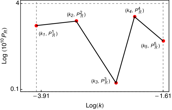
Figure 1: Illustration of the methodology for a 5 knots case ($N=5$). We fix both $k_{1}=0.02\text{ h}\text{ Mpc}^{-1}$ and $k_{N}\equiv k_{5}=0.2\text{ h}\text{ Mpc}^{-1}$, which correspond to the largest and smallest scales of the catalogue. The sampled parameters are the $\text{log}(x)$ (see next paragraph) for each {$k_{2}$,$k_{3}$,$k_{4}$} and the logarithms of {$P_{\mathcal{R}}^{1}$,$P_{\mathcal{R}}^{2}$,$P_{\mathcal{R}}^{3}$,$P_{\mathcal{R}}^{4}$,$P_{\mathcal{R}}^{5}$}. We impose a flat prior with the upper and lower limits for all the $\{k_{i},P_{\mathcal{R}}^{i}\}$ coordinates according to the dashed lines: scales within the catalogue limits and $P_{\mathcal{R}}$ from $1.0\times 10^{-10}$ to $5.6\times 10^{-9}$.

The $k$ coordinates are not directly sampled. For each knot $i$ we sample the pair of quantities $\{x_{i},\text{log}(P_{\mathcal{R}}^{i})\}$, where the coordinates $x$ are a normalization of the catalogue scales $\text{log}(k)$, with $x=0$ and $x=1$ corresponding to $\text{log}(k_{1})$ and $\text{log}(k_{N})$ respectively. The outermost knots with scales $x_{1}$ and $x_{N}$ are fixed, while their $\text{log}(P_{\mathcal{R}}^{1})$ and $\text{log}(P_{\mathcal{R}}^{N})$ are sampled. All other intermediate scales $x_{i}$ fall into the (0,1) range. This parameter space is degenerated since any permutation of the knots gives the same reconstruction. This label switching problem is avoided with a transformation of the scales $x_{i}$ into ordered scales $x^{\prime}_{i}$. We discuss this problem and its solution in section 7.1. Once the normalized coordinates are ordered we can unambiguously map them back to physical scales $k$. In a generic scenario with $N$ knots we have to sample $N-2$ values of $x$ (or equivalently $k$) and $N$ values of $P_{\mathcal{R}}$, resulting in a total of $2N-2$ variables. The particular case of the SM (represented by a power law power spectrum) is reproduced using only two variables $P_{\mathcal{R}}^{1}$ and $P_{\mathcal{R}}^{2}$. This corresponds to the $N=2$ configuration in our methodology. Furthermore, sampling just a single knot in the $N=1$ scenario, $P_{\mathcal{R}}^{1}$, corresponds to a scale invariant Harrison-Zeldovich primordial power spectrum ($n_{s}=1$).

We assume that the $P_{\mathcal{R}}^{(0)}(k)$ is given in the scale range $k\in[0.02,0.2]\text{ h}\text{ Mpc}^{-1}$, divided in 92 elements with uniform logarithmic steps $\text{Log}(\Delta k)=0.02$. For high-$z$ objects this range is extended to $k=0.47\text{ h}\text{ Mpc}^{-1}$, with the same step. We adopt flat priors for both $P_{\mathcal{R}}$ in a wide range $P_{\mathcal{R}}\in[0.10,5.60]\times 10^{-9}$ and $x\in[0,1]$.

We reconstruct $P_{\mathcal{R}}(k)$ by maximizing a likelihood function that quantifies the agreement between the theoretical model of the monopole galaxy power spectrum $P^{(0)}_{g}(\mbox{model})$ and the one derived from the data catalog $P^{(0)}_{g}(\mbox{data})$. We evaluate the spectra for different bins of redshift $z$ and for each value of the catalogue scale grid. The likelihood $\mathcal{L}$ used in this analysis follows a multi-variable Gaussian form:

$$-2\mbox{Log}(\mathcal{L})=\sum_{i=1}^{i=Z}\sum_{j=1}^{j=K}\left[x_{ij}^{2}\frac{1}{\sigma^{2}_{ij}}+\mbox{Log}\left(\sigma^{2}_{ij}\right)\right],$$ (2.2)

where $x_{ij}\equiv[P^{(0)}_{g,ij}(\mbox{model})-P^{(0)}_{g,ij}(\mbox{data})]$; $i$ is the index for the different redshift bins, with $Z$ the total number of redshift bins for the catalogue; $j$ is the index accounting for the scales, with $K$ the total number of scales for that catalogue; and $\sigma_{ij}^{2}$ is the variance calculated from $P^{(0)}_{g,ij}(\mbox{model})$, as explained in the next section. In general a covariance matrix is needed. Since we consider uncorrelated scales and redshift bins, it is diagonal and we can reduce it to its variance elements. The reconstructions of $P_{\mathcal{R}}(k)$ are obtained from the values of $P^{(0)}_{g,ij}(\text{model})$ that maximize $\mathcal{L}$.

We summarize our sample selection criteria in section 7.2. After the sampling is done and a first set of reconstructions is chosen, we get a large number of reconstructions of the primordial power spectrum for each number of knots configuration, each one denoted as $P_{\mathcal{R},j,N}(k)$. Each reconstruction has associated its own normalized importance weight $\omega_{j,N}$.

We can merge all the reconstructions coming from any $N$ configuration by reconstructing a marginalized probability over $N$ of $P_{\mathcal{R}}(k)$. Since CosmoChord calculates the individual evidences $Z_{N}$, the marginalization is done by combining all reconstructions from all $N$ with a new set of evidence-dependent weights $q_{j,N}$:

$$q_{j,N}=\omega_{j,N}\frac{Z_{N}}{\sum_{M}Z_{M}}.$$ (2.3)

We can interpret each weight $q_{j,N}$ as the joint probability of both the chain $j$ and the $N$ knots configuration. This joint probability is the product of two factors: the conditional probability of the chain $j$ given $N$, $\omega_{j,N}$, and the probability of the $N$ configuration given by the normalized evidence. Their corresponding reconstructions $P_{\mathcal{R},{j,N}}(k)$ have an associated probability $q_{j,N}$, from which we determine the confidence intervals of $P_{\mathcal{R}}(k)$ according to the $q_{j,N}$ distribution.

We test our method on simulated data with different $P_{\mathcal{R}}(k)$, based on the power spectrum templates given in eq. 7.2 and eq. 4.1 and described in [57, 19, 20, 21]. These templates cover a broad range of theoretical motivated models. We focus on the small scale regime where the LSS surveys can achieve higher precision than the CMB experiments. We also apply our methodology to real observational data obtained from the Sloan Sky Digital Survey Luminous Red Galaxy data release 4 (SDSS LRG 04). We use two statistical tests to analyze the reconstructed spectra and assess possible deviations from the power law assumption, as explained below.

2.2 Feature detection from $P_{\mathcal{R}}(k)$ reconstructions

To detect features in the reconstructed $P_{\mathcal{R}}(k)$, we perform two tests for each reconstruction. The first test is a global one based on the comparison of the evidence ratios and the second test is a novel local one based on a hypothesis test. Both tests are applied to the comparison of the $N=2$ and the marginalized probability over $N$ reconstructions.

2.2.1 Global test

Evidence comparison for model selection and comparison with the SM is widely used [82]. In this work we use the evidence ratio $Z_{\text{max}}/Z_{2}$, where $Z_{2}$ is the evidence of the primordial power law reconstruction and $Z_{\text{max}}$ is the highest value among the evidences $Z_{N}$ except $Z_{2}$. The $Z_{\text{max}}/Z_{2}$ ratio measures how a power law primordial spectrum compares with a different knot number configuration spectrum with the highest evidence. We have checked that the sampling errors in the estimates of the evidences are less than 1% for values above 1% of the maximum evidence. In this way, we are confident in the application of the Jeffreys criterion [83] for quantifying the feature detection status.

This global test provides an effective way of measuring how different $N$ configurations compare when reconstructing $P_{\mathcal{R}}(k)$. The detection of a feature can be claimed, but with only this analysis we could not identify at which scales the deviations are more significant. To locate the deviations at the scales they occur, we use a local test, explained below.

2.2.2 Local test

We perform another complementary analysis of the $P_{\mathcal{R}}(k)$ reconstructions. This analysis is a novel approach for detecting features in $P_{\mathcal{R}}(k)$, providing insights about possible features present in $P_{\mathcal{R}}(k)$ in a localized way, since it enables us to identify the scales at which the deviations occur.

The local test is a hypothesis test applied to the distributions of the $N=2$ and the marginalized probability over $N$ reconstructions for each value of the catalogue grid scale. The details of the hypothesis test can be found in [84]. The significance level considered for all the tests is $\alpha=0.05$. The power of the test $1-\beta$ quantifies the separation between both distributions providing a measure of the significance of the deviation from the power law.

We establish the feature detection status using the following thresholds for the power of the test: $1-\beta>0.95$ at any $k$ indicates that both distributions are separated enough to consider the feature detection at that scale; $0.95>1-\beta>0.5$ shows a hint of a feature; and $0.5>1-\beta$ shows no evidence of the presence of a feature.

The global test is a statistically more robust test for feature detection, since it compares evidences computed for all the scales and it is less sensitive to fluctuations, but the local test enables us to locate features at certain scales $k$, providing an indicator for the existence and location of features in $P_{\mathcal{R}}$. We apply both test to all our reconstructions, exploiting the complementary information that both methods offer.

3 Galaxy power spectrum simulations: survey specifications and modelling

In order to test the methodology we apply it to simulations. In this work we simulate galaxy power spectra using galaxy clustering modeling. Recent galaxy clustering models account for various effects, such as Baryon Acoustic Oscillations (BAO) modelling [85, 86], non-linear corrections [87, 88], the Fingers of God [89] and Alcock-Paczynski [90, 91] effects, or complex shapes of the redshift-space power spectrum [92, 93, 94, 95]. A simple BAO modelling and non-linear corrections will be considered for the SDSS LRG real data application in section 5.

All the simulations described in this section have been done assuming a linear regime using a Kaiser redshift-space power spectrum, focusing on testing our methodology, without aiming for a state of the art modelling of the simulated data. A comparison of the deviations w.r.t. non-lineal modelling [86, 87] at scales $k\sim 0.1\text{ h}\text{ Mpc}^{-1}$ shows an underestimation of power of $\approx 30\%$. However, this underestimation in the modelling at the smallest scales is not biasing our results since it is present coherently in both the model and the simulations. Therefore, we consider that for our analysis, scales up to $k=0.2\text{ h}\text{ Mpc}^{-1}$ are adequate enough for our purposes. When dealing with high-$z$ objects we extend the smallest scales considered up to $0.47\text{ h}\text{ Mpc}^{-1}$, since non-linear effects happen at smaller scales at high $z$. We explain how our simulations are done in the rest of this section.

3.1 Simulated surveys specifications

We differentiate between low and high redshift objects: Luminous Red Galaxies (LRGs) and Emission Line Galaxies (ELGs) are examples of the former, while Quasi-Stellar Objects (QSOs) of the later. Typical redshifts covered by current planned surveys for galaxies are $z\lesssim 1$ whereas for QSOs $z\sim 2$. For both types of objects, we choose a redshift binning with a step $\Delta z=0.2$ and evaluate the power spectra at the central values of the bins.

We estimate mean values of the photometric redshift error $\delta_{z}$ from J-PAS representative data [96, 97, 98] by weighting the $\delta_{z}$ associated to each redshift bin with the densities derived below (see table 1). For low-$z$ objects, a low photometric error of $\delta_{z}=0.0038$ is obtained using the 30% best determined redshifts, and a high photometric error of $\delta_{z}=0.039$ is derived when the 50% best ones are considered. For high redshift objects a single value $\delta_{z}=0.0036$ is obtained considering all the QSOs.

The observed sky fraction assumed for the simulations is $f_{\mbox{sky}}=0.2575$, equivalent to an area of $10620\text{ deg}^{2}$, an intermediate value between expected $f_{\mbox{sky}}$ of future LSS catalogues, such as J-PAS with an area of $8500\text{ deg}^{2}$ [43], DESI with $14000\text{ deg}^{2}$ [44], or Euclid with $15000\text{ deg}^{2}$ [45].

3.1.1 Bias model

Galaxy biasing is a complex process that needs to be modeled to extract cosmological information from current and future LSS data. Different tracers of the LSS exhibit different bias, which can be derived from bottom-up or top-down approaches, with local or non-local bias, and considering non-linearities. In this work we focus on spectra with scales larger than $0.2\text{ h}\text{ Mpc}^{-1}$. For these scales we assume scale independent bias models and neglect the effects of scale-dependent deviations in the bias.

For the low-$z$ galaxies we adopt the relation in [99]:

$$b(z)=\frac{b_{0}}{D(z)}.$$ (3.1)

We assume a ELG-like biasing, with $b_{0}=0.84$ following [100] and consistent with [43].

The QSO bias model is obtained by matching the integrated correlation function for QSOs with the expected one for the WMAP/2dF cosmology [101]. The model is parametrized as [102]:

$$b(z)=0.53+0.289(1+z)^{2}.$$ (3.2)

Galaxy clustering observables require non-linear and non-local bias models for a broad range of scales, as linear and scale independent bias models are inadequate [103]. For instance, the power spectrum multipoles and the bispectrum of BOSS CMASS DR11 galaxies were analyzed using such models [104, 105, 106], and they are also necessary for more recent galaxy clustering data. However, the main goal of this work is to test our reconstructions methodologically rather than to model galaxy clustering with the latest techniques.

3.1.2 Number density of galaxies

To estimate the uncertainties in the monopole galaxy power spectrum, we need the densities of the catalogue objects, which depend on both the redshift and the photometric error, i.e. $\hat{n}(z,\sigma_{z})$, where $\sigma_{z}=\delta_{z}(1+z)$. We use realistic values of densities $\hat{n}$ for both low-$z$ and high-$z$ power spectrum simulations, based on the expectations of the J-PAS collaboration [43]. To estimate the densities we follow [96] for low redshift (ELGs) and [97, 98] for high redshift (QSOs). The values of the densities that we use in our power spectrum model are obtained by fitting the density data with the following function for $\hat{n}(z)$:

$$\hat{n}(z)=C_{0}z^{\alpha}\text{e}^{-\left(\frac{z}{z_{0}}\right)^{\beta}}.$$ (3.3)

By evaluating that function at the central values of the $z$-bins for each object type, we obtain the densities required. The parameters $\{C_{0},z_{0},\alpha\}$ are considered as free parameters, with $\beta=3/2$ [100]. Table 1 shows the values of the densities used for each $z$-bin.

Low-z	Low-$\delta_{z}$	High-$\delta_{z}$
$z$-bin	$\hat{n}/10^{-3}h^{3}\text{ Mpc}^{-3}$	$\hat{n}/10^{-3}h^{3}\text{ Mpc}^{-3}$
$0.1$	12	48
$0.3$	6.1	25
$0.5$	2.4	10
$0.7$	0.75	3.2
$0.9$	0.19	0.87

High-z	Low-$\delta_{z}$
$z$-bin	$\hat{n}/10^{-3}h^{3}\text{ Mpc}^{-3}$
$1.7$	0.030
$1.9$	0.035
$2.1$	0.037
$2.3$	0.037
$2.5$	0.033
$2.7$	0.028
$2.9$	0.023

Table 1: Densities $\hat{n}$ in units of $10^{-3}\text{ h}^{3}\text{ Mpc}^{-3}$ of low (left table) and high (right table) redshift objects for each bin of redshift $z$. The values of the densities depend on the photometric error $\delta_{z}$, and are estimated for low-$z$ [96] and high-$z$ [97, 98] objects using eq. 3.3.

3.2 Construction of the monopole galaxy power spectrum

Our observable of interest is the monopole galaxy power spectrum $P_{g}^{(0)}(k,z)$, from which we reconstruct $P_{\mathcal{R}}(k)$ using the likelihood of eq. 2.2. We estimate the mean value $\bar{P_{g}}^{(0)}(k,z)$ following the model in [100], which is based on [107] and inspired by the Kaiser model [92]. This model accounts for redshift space distortions at a basic level, with a Gaussian uncertainty in its radial position.

$\bar{P_{g}}^{(0)}(k,z)$ is obtained through the matter power spectrum, which depends on the primordial power spectrum and a transfer function $T(k)$ that is sensitive to the cosmology. We adopt cosmological parameters that are consistent with Planck DR3 [108]: $H_{0}=66.7\text{ km/(s Mpc)}$, $\Omega_{b}=0.004869$, $\Omega_{c}=0.02655$, $A_{s}=2.0905\times 10^{-9}$, $n_{s}=0.9626$, $k_{0}=0.05\text{ Mpc}^{-1}$ and $\tau=0.0522$. We compute $T(k)$ with CAMB [109]. We describe the construction of the galaxy power spectrum below.

We start by choosing a primordial power spectrum $P_{\mathcal{R}}(k)$. We will consider either the SM power law $A_{s}\left(\frac{k}{k_{0}}\right)^{n_{s}-1}$ or various templates with deviations from the power law, all based on physically motivated models, such as the ones in eq. 7.2, that we explain in section 7.3, or in eq. 4.1.

We construct the linear matter power spectrum $P_{m}(k)$ as:

$$P_{m}(k)=2\pi^{2}h^{4}T^{2}(k)kP_{\mathcal{R}}(k).$$ (3.4)

A simple way to estimate a galaxy power spectrum $\bar{P_{g}}(k)$ is to assume that it is proportional to the matter power spectrum. The proportionality is taking into account through the bias $b$:

$$\bar{P_{g}}(k)=b^{2}P_{m}(k).$$ (3.5)

This simple method is not accurate enough to describe a galaxy power spectrum [104], not even in the linear regime. We proceed as in [100] and consider the following more realistic description:

$$\bar{P_{g}}(k,\mu,z)=\left[A(z)+R(z)\mu^{2}\right]^{2}\frac{P_{m}(k)}{\sigma_{8}^{2}}e^{-k^{2}\mu^{2}\sigma_{r}^{2}(z)},$$ (3.6)

with $\mu$ being the cosine of the angle between the wavevector $\vec{k}$ and the line of sight, the function $A(z)=D(z)\mbox{ }b(z)\mbox{ }\sigma_{8}$ includes the bias $b(z)$ from the previous subsection, and the function $R(z)=D(z)\mbox{ }f(z)\mbox{ }\sigma_{8}$ involves the growth function $f(z)$ and the growth factor $D(z)$. The model has a $\mu$ dependence in the term $R(z)$ and the exponential term $e^{-k^{2}\mu^{2}\sigma_{r}^{2}(z)}$. This exponential accounts for a reduction of power due to uncertainties induced by the photometric error of the measurements through the parameter $\sigma_{r}=\frac{\delta_{z}(1+z)}{H(z)}$, with $H(z)=H_{0}E(z)$ the Hubble function. The power suppression results from the convolution of the line of sight comoving position $r$ with a Gaussian $\text{e}^{\frac{-(\Delta_{r})^{2}}{2\sigma_{r}^{2}}}$. The function $E(z)$ is defined as:

$$E(z)=\sqrt{\Omega_{m}(1+z)^{3}+(1-\Omega_{m})},$$ (3.7)

and the growth factor $D(z)$ is calculated as:

$$D(z)=\exp\left[\int_{0}^{N(z)}f\left(N^{\prime}\right)dN^{\prime}\right],$$ (3.8)

where $N(z)=-\log(1+z)$. The growth function $f(z)$ is estimated as:

$$f(z)=\left(\Omega_{m}(1+z)^{3}\frac{1}{E^{2}(z)}\right)^{\gamma},$$ (3.9)

being $\gamma=0.545$ the growth index. The $\ell$-multipoles of $\bar{P_{g}}\left(k,\mu,z\right)$ can be computed as:

$$\bar{P_{g}}^{(\ell)}(k,z)=\frac{(2\ell+1)}{2}\int_{-1}^{1}\bar{P_{g}}\left(k,\mu,z\right)\mathcal{L}_{\ell}(\mu)d\mu,$$ (3.10)

with $\mathcal{L}_{\ell}(\mu)$ the Legendre polynomial of degree $\ell$. An analytical expression for the monopole ($l=0$) is derived:

$$\begin{split}\bar{P_{g}}^{(0)}(k,z)=\frac{P_{m}}{8k^{5}\sigma_{8}^{2}\sigma_{r}^{5}}\Bigl{(}\sqrt{\pi}\text{Erf}(k\sigma_{r})\left[4A(z)^{2}k^{4}\sigma_{r}^{4}+4A(z)k^{2}R(z)\sigma_{r}^{2}+3R(z)^{2}\right]\\ -2kR(z)\sigma_{r}e^{-k^{2}\sigma_{r}^{2}}\left[2k^{2}\sigma_{r}^{2}(2A(z)+R(z))+3R(z)\right]\Bigl{)}.\end{split}$$ (3.11)

Eq. 3.6 does not capture the redshift space power spectrum accurately, as it neglects the non-linear effects that affect the linear scales [110, 111]. More advanced models take into account these non-linearities, such as the ones in [92, 93, 94]. We will not consider them here, but would be required for state of the art surveys.

The expected value of the monopole galaxy power spectrum at wavenumber $k$ and redshift $z$ is given by eq. 3.11. To estimate its uncertainties, its variance matrix has to be computed. We follow the method in [112], which requires an additional term: the Fourier number of modes assigned to the $k$-shell $N_{k}(z)$. For this, we define the comoving distance as:

$$\chi(z)=\frac{1}{H_{0}}\int_{0}^{z}\frac{1}{E(z^{\prime})}dz^{\prime}.$$ (3.12)

Then we estimate the volume in a redshift bin of central value $z$ and upper and lower limits $z_{+}$ and $z_{-}$:

$$V_{\alpha}(z)=\frac{4}{3}\pi f_{\mbox{sky}}\left[\chi^{3}(z_{+})-\chi^{3}(z_{-})\right].$$ (3.13)

The number of Fourier modes $N_{k}$ inside a $k$-shell between $k_{+}$ and $k_{-}$ for the redshift bin $z$ are:

$$N_{k}(z)=\frac{V_{\alpha}(z)}{(2\pi)^{3}}\frac{4}{3}\pi(k_{+}^{3}-k_{-}^{3}),$$ (3.14)

where $k_{+}$ and $k_{-}$ represent the upper and lower limits of the bin associated to $k$. The number of Fourier modes contributes to the sampling variance effect. The shot noise is included by the inverse of the density $\hat{n}$. Then, the variance accounting for both effects can be written as:

$$\sigma^{2}(k,z)=2\frac{[\bar{P_{g}}^{(0)}(k,z)+\frac{1}{\hat{n}}]^{2}}{N_{k}(z)}.$$ (3.15)

The standard deviations are considered as the uncertainties in our observable monopole galaxy power spectrum, i.e. $\delta\bar{P_{g}}^{(0)}(k,z)=\sigma(k,z)$.

The sample volume at the largest scales and the dominance of non-linear effects at the smallest ones determine the scales at which we apply our methodology. A scale range of $k\in[0.02-0.2]\text{ h}\text{ Mpc}^{-1}$ for low-$z$ objects and $k\in[0.02-0.47]\text{ h}\text{ Mpc}^{-1}$ for high-$z$ ones is used, as non-linear effects appear at smaller scales for high redshifts. The noise properties also vary with scale $k$: the sampling variance is higher at large scales and the shot noise tends to dominate at small ones. The variation of the signal to noise ratio with scale $k$ can be seen in figure 2, presented in the next subsection for different redshifts.

We use this model of the monopole galaxy power spectrum to generate simulations and test our methodology for the reconstruction of the primordial one in section 4.

3.3 Signal to noise analysis

In the previous section we have described the observed power spectrum model, the physical properties of the objects and the characteristics of the survey. We now study the expected signal to noise ratio $S/N$ for each clustering scenario. The sensitivity of our methodology to power deviations will depend on the $S/N$ of $P_{g}^{(0)}(k_{i},z_{j})$ for the different objects, given by $S/N(k,z)=\frac{\bar{P}_{g}^{(0)}(k,z)}{\sigma(k,z)}$.

In figure 2 the $S/N$ as a function of the scale $k$ is represented for the SM. This figure reflects the dominance of the sampling variance for most of the redshift bins of the low-$z$ objects (top panels) and the shot noise dominance for the high-$z$ objects (bottom panel). In the low-$z$ scenario the shot noise term $\frac{1}{\hat{n}}$ in eq. 3.15 is subdominant for the majority of redshift bins, except for the highest ones that have the lowest densities (listed in table 1) at small scales. Only for the $z=0.7$ and $z=0.9$ bins the shot noise dominates over $\bar{P}_{g}^{(0)}$ producing a slight reduction in the $S/N$ at the smallest scales. The number of modes $N_{k}(z)$ for a certain $k$ (given by the volume included in a redshift bin) leads to a very different sampling variance between redshift bins, explaining the low $S/N$ at the smallest bins. In the case of low-$z$ with high-$\delta_{z}$ (top right panel), the shot noise has a slightly higher effect than for low $\delta_{z}$ due to the reduction of $\bar{P}_{g}^{(0)}$ (implying a reduction in both the signal and the sampling variance), caused by the higher photometric error (see eq. 3.6). For the high-$z$ objects (plotted in the bottom panel of figure 2) the shot noise dominates at all scales due to their lower densities compared to the low-z ones. As a consequence, those bins with the highest densities will have the smallest noise and the highest S/N. The volume differences between redshift bins are much smaller than in the case of the low-z objects, implying similar sampling variance among them.

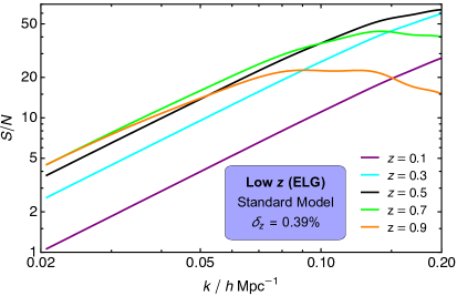
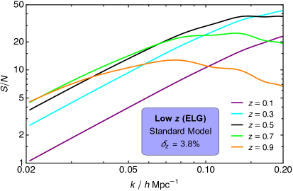
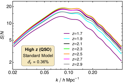
Figure 2: Signal to noise ratios $S/N(k)$ for the SM at different redshift bins for different scenarios. Top panels: for low-$z$ objects with low (left) and high (right) $\delta_{z}$. Bottom panel: for high-$z$ objects.

In section 4 we apply the methodology to low-$z$ objects for two conservative redshift bins centred at $z=0.1$ and $z=0.9$ that are limited by the sampling variance and the shot noise, respectively. We also apply to high-$z$ simulations where we consider the favorable bin $z=2.3$ having the highest $S/N$ of all the bins up to $k=0.15\text{ h}\text{ Mpc}^{-1}$, and for smaller scales is slightly lower than for the $z=2.5$ bin where the $S/N$ is maximum. In addition, we combine all the redshift bins for either the low-$z$ or the high-$z$ objects. Since we treat the redshift bins as uncorrelated, the resultant $S/N$ is enhanced, leading to the most favorable scenario in order to test our methodology, in contrast to the conservative cases. In this way we can obtain the minimum amplitude of features that the method is able to detect at low or high redshift.

4 Application to simulated spectra

In this section we apply the methodology to simulations of different observational scenarios, characterized by the monopole galaxy power spectrum model $\bar{P_{g}}^{(0)}(k_{i},z_{j})$ at a given scale $k_{i}$ and redshift bin $z_{j}$, and the survey and object specifications described in section 3. We simulate the “observed” monopole power spectrum at a scale $k_{i}$ and redshift bin $z_{j}$, $P_{g}^{(0)}(k_{i},z_{j})$, by drawing random samples from a Gaussian distribution with mean $\bar{P_{g}}^{(0)}(k_{i},z_{j})$ and standard deviation $\delta\bar{P_{g}}^{(0)}(k_{i},z_{j})=\sigma(k_{i},z_{j})$ obtained from the variance matrix given by eq. 3.15. We consider a low-$z$ galaxy survey with two photometric redshift errors, a low and a high $\delta_{z}$, and a high-$z$ QSO survey with only a relatively low $\delta_{z}$ (see section 3.1).

First we test the methodology with SM simulations, i.e. assuming a power law for the primordial power spectrum $P_{\mathcal{R}}(k)$. Then we apply the methodology to simulations with primordial features. We consider two features templates, a local and a global one. From the local template given in eq. 7.2, we first generate a feature that consists of a 5% bump in power at $k\approx 0.2\text{ h}\text{ Mpc}^{-1}$ (see figure 6). Using the same template, we also generate a second local feature having an oscillatory behaviour with excess and deficit of power of approximately 10% at the maximum and minimum of the oscillation (see figure 10). We also apply the methodology to a different feature template, namely a global log-log oscillatory feature with oscillations at all scales (see eq. 4.1). We consider three amplitudes for the global template, corresponding to approx. 10%, 3% and 1.5% power deviations from the featureless primordial power law. Finally, we also explore the smallest power deviations that we are able to detect with this methodology for each of the three features considered. This is achieved by combining all the redshift bins for either low or high-$z$, since the independence of the redshift bins results in a clear enhancement of the $S/N$ (see figure 2). We have checked that different realizations of the same observational scenario provide very similar reconstructions leading to the same feature detection results derived from the global and local tests.

4.1 Standard Model

The Standard Model simulations are performed considering $P_{\mathcal{R}}(k)$ as a power law $\mathcal{P}_{\mathcal{R}}^{\text{SM}}(k)=A_{s}\left(\frac{k}{k_{0}}\right)^{n_{s}-1}$. We consider simulations of $P_{g}^{(0)}(k)$ at the low-$z$ bin $z=0.1$. This is a conservative scenario: despite having the lowest shot noise contribution, the sampling variance dominates at all scales, producing low $S/N$ values. The $P_{\mathcal{R}}(k)$ reconstructions for the high-$z$ $P_{g}^{(0)}(k)$ simulations are applied to the $z=2.3$ bin, a favorable case since it has the minimum shot noise and the highest $S/N$ values for almost all the scale range (see figure 2).

As shown in figure 3, the power of $P_{g}^{(0)}(k)$ is lower in the high-$\delta_{z}$ realization than in the low-$\delta_{z}$ one, with a factor of 10 difference at the smallest scales. The sampling variance is similar for both cases, while the shot noise has a slightly larger impact in the high-$\delta_{z}$ realization. These effects agree with the $S/N$ analysis in section 3. $P_{g}^{(0)}(k)$ has more power for the high-$z$ objects than for the low-$z$ objects, even with the low $\delta_{z}$.

As expected, all the evidences of the reconstructed spectra peak at the 2 knots case, $Z_{2}$, and exhibit a quasi-exponential decay with increasing $N$, as shown in figure 4. For the low-$z$ scenarios $Z_{3}$ is almost a factor of 5 smaller than $Z_{2}$, while for the high-$z$ case it is approximately a factor of 10 smaller. The recovery of the power law is clear in all three cases, with negative feature detection as summarized in the second column of table 2.

Also the hypothesis test do not show any local deviations between the marginalized and the $N=2$ case, as displayed in figure 5. The value of $1-\beta$, is very small for both the low-$z$ ($<0.15$) and the high-$z$ ($<0.05$) objects at all scales, showing a very good consistency between the $N=2$ and the marginalized reconstruction. The contours are similar for both low-$z$ reconstructions, showing a large widening at the largest scales due to the high sampling variance. In contrast, for the high-$z$ scenario they are narrower at the largest scales and wider at the smallest ones $k\approx 0.5\text{ h}\text{ Mpc}^{-1}$, due to the dominance of the shot noise.

The results obtained for the case of the SM show the preference for the power law, with a good recovery of the input values for the parameters $\{A_{s},n_{s}\}$ with the global test and no deviation detected with the local one, validating the performance of the proposed methodology.

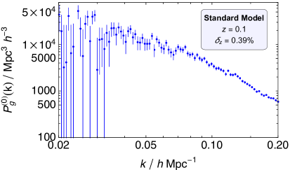
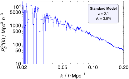
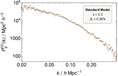
Figure 3: Simulated monopole galaxy power spectrum $P_{g}^{(0)}(k)$ performed for the SM, i.e. with its $P_{\mathcal{R}}(k)$ being the power law. Top panel: low-$z$ low-$\delta_{z}$ (left) and high-$\delta_{z}$ (right) simulations. Bottom panel: high-$z$ simulation. Note how on this scenario the range of scales is extended up to $k=0.47\text{ h}\text{ Mpc}^{-1}$.

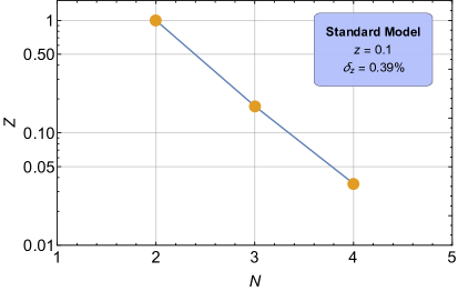
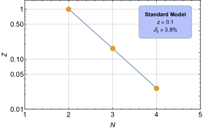
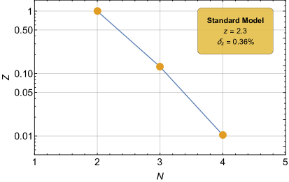
Figure 4: Evidence $Z$ of the Standard Model reconstructions for each of the $N$ knots configuration considered for the low-$z$ low-$\delta_{z}$ (top left), low-$z$ high-$\delta_{z}$ (top right) and high-$z$ (bottom) cases.

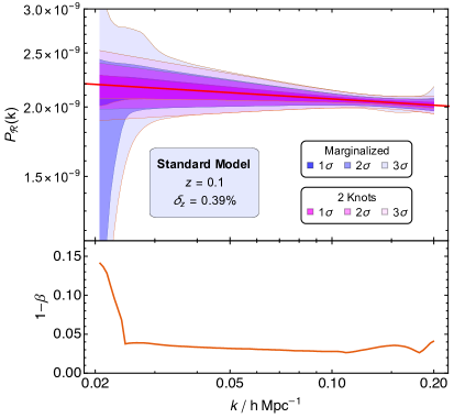
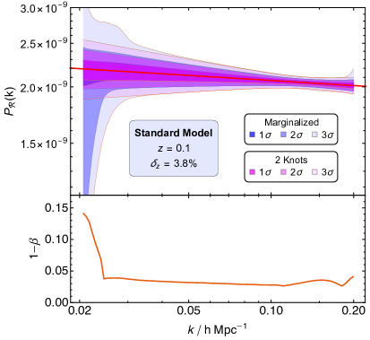
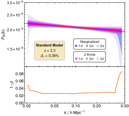
Figure 5: Contours of the $P_{\mathcal{R}}(k)$ reconstructions for the SM simulations for the $N=2$ case (magenta) and for the case of marginalized probability over $N$ knots (blue). We include in red the power law that sourced the simulations. In the bottom panel of each figure the values of the power $1-\beta$ obtained from the hypothesis test are plotted. Top left figure: low-$z$ low-$\delta_{z}$ simulations. Top right figure: low-$z$ high-$\delta_{z}$ simulations. Bottom figure: simulations in the high-$z$ scenario.

4.2 Local bump feature

We study a local feature in $P_{\mathcal{R}}(k)$ following the template in eq. 7.2. We tune the parameters of this template to have a bump at $k\approx 0.20\text{ h}\text{ Mpc}^{-1}$ with a 5% power excess relative to the featureless model. The primordial spectrum for this bump feature, and the parameters used to generate it, are shown in figure 6.

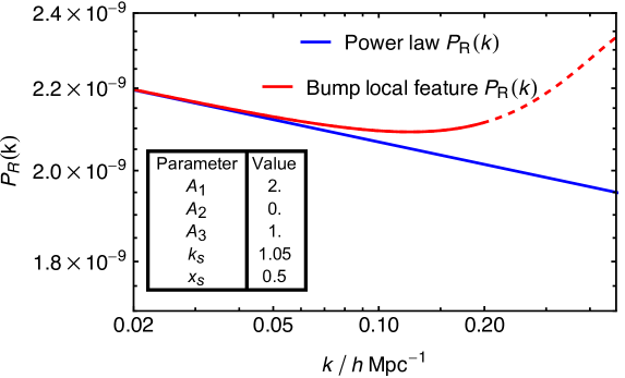
Figure 6: Local bump feature model of the primordial power spectrum (solid red for low-$z$ scales and dashed red for the extended high-$z$ ones) and the power law primordial power spectrum (blue). The parameters used to generate the bump feature are given in the table inside the figure. Note the increase of power at the scale $k=0.20\text{ h}\text{ Mpc}^{-1}$ where it reaches 5%. At large scales, the feature model tends to the SM power law.

We use the same redshift bins than for the SM. The corresponding simulated power spectra show the slight increase of power at the smallest scales of the template, as plotted in figure 7. For low-$z$ objects, the power increase is about 5%, whereas for the high-$z$ ones, which have a larger scale range up to $k=0.47\text{ h}\text{ Mpc}^{-1}$, it reaches 10% compared to the SM power law.

The global test for the bump feature is based on the ratio of evidences that are shown in figure 8. For the low-$z$ objects the evidence $Z$ peaks at $N=2$ and falls with $N$ in a similar way to the SM case studied in the previous section. For the high-$z$ objects and considering only a single redshift bin $Z_{3}$ is almost twice as high as in the case of the SM and $Z_{4}$ four times higher. Nevertheless, the maximum evidence is still obtained for $N=2$. In the bottom right panel we show the results of the global test applied to the combined redshift bins for the high-$z$ reconstructions. With this combination the evidence is maximum at $N=3$, and $Z_{4}$ takes the second highest value which is $\approx 10\%$ smaller. At $N=2$ it takes a very small value of $\sim 10^{-4}$, which strongly disfavours the power law pointing to a decisive feature detection. Bumps with amplitudes 2% and 5% are detected with substantial evidence when combining all the redshift bins in the high-$z$ and low-$z$ scenarios, respectively.

The low-$z$ reconstructions shown at the top panels of figure 9 follow a power law, as the global tests indicate, but with a higher $n_{s}$ and slightly lower $A_{s}$ than in the featureless scenario. This more tilted power law accounts for the bump at the smallest scales, in such a way that $1-\beta$, below 0.20 at all scales, do not indicate the presence of any local deviation.

The high-$z$ reconstructions in the bottom panels of figure 9 differ from the low-$z$ ones. The left panel shows the case with only the $z=2.3$ bin, and the right panel with all the seven redshift bins combined. When using only the $z=2.3$ bin, the contours of the $N=2$ and marginalized reconstructions are much wider and strongly overlap, making them indistinguishable at the smallest scales, as confirmed by the hypothesis test. When combining all the high-$z$ redshift bins (bottom right panel of figure 9) the power law and marginalized probability over the $N$ knot distributions are clearly separated, as shown by the contour shapes and the hypothesis test values, with $1-\beta>0.90$ at multiple scales. Thus, the local test indicates feature detection (see third column of table 2). Note also that the reconstructions become sharper when data from different redshift bins are combined.

To summarize, for the bump feature template the low-$z$ reconstructions do not show any evidence of the feature. For the high-$z$ reconstructions, using just one bin also fails to detect the feature. Only when combining all the seven high-$z$ redshift bins we can clearly identify the excess of power caused by the feature, indicating a decisively preference for a primordial power spectrum with 3 knots compared to the SM power law, as shown in the third column of table 2.

The application of our methodology to the bump feature provides the same qualitative results as for the SM case, except for one case: when combining all the information of the redshift bins in the high-$z$ scenario. Moreover, we have looked for the minimum amplitude that can be detected in this most favorable case. The result is that substantial detection can be achieved for a minimum amplitude of $2\%$.

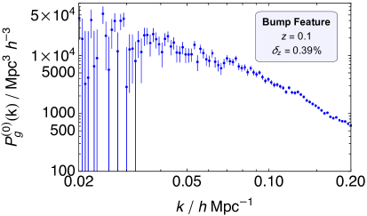
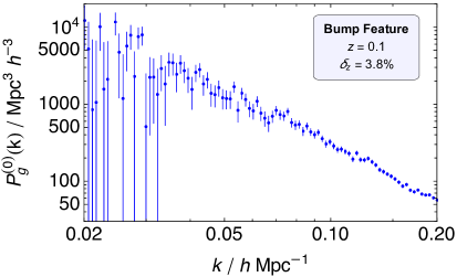
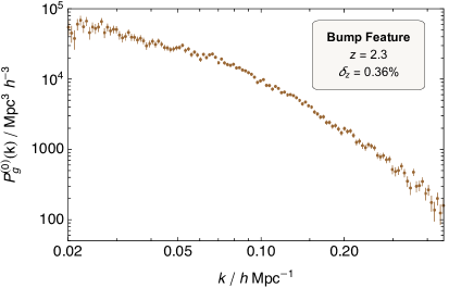
Figure 7: Simulated monopole galaxy power spectrum $P_{g}^{(0)}(k)$ performed for the bump feature template. Top panel: low-$z$ low-$\delta_{z}$ (left) and high-$\delta_{z}$ (right) simulations. Bottom panel: high-$z$ single redshift bin simulation.

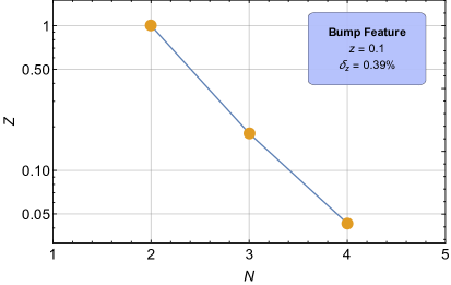
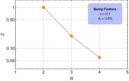
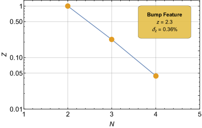
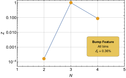
Figure 8: Evidence $Z$ of the local bump feature template reconstructions for each of the $N$ knots configurations considered in the low-$z$ low-$\delta_{z}$ (top left), low-$z$ high-$\delta_{z}$ (top right), high-$z$ for one single redshift bin (bottom left) and high-$z$ combining all the redshift bins (bottom right) scenarios.

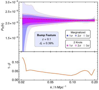
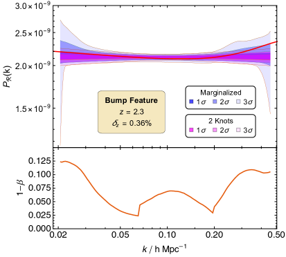
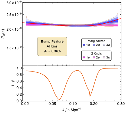
Figure 9: Contours of the $P_{\mathcal{R}}(k)$ reconstructions for the bump feature simulations for the $N=2$ case (magenta) and for the case of marginalized probability over $N$ knots (blue). We include in red the bump feature template that sourced the simulations. In the bottom panel of each figure the values of the power $1-\beta$ obtained from the hypothesis test are plotted. Top left figure: low-$z$ low-$\delta_{z}$ simulations. Top right figure: low-$z$ high-$\delta_{z}$ simulations. Bottom left figure: simulations in the high-$z$ scenario for one single redshift bin. Bottom right figure: simulations in the high-$z$ scenario combining all the redshift bins.

4.3 Local oscillatory feature

We examine how our methodology performs with another local feature in the primordial power spectrum $P_{\mathcal{R}}(k)$. The template for generating this feature is the same as for the bump one (see eq. 7.2), we now choose values of the different parameters to generate a power excess and a deficit of amplitude $\approx 10\%$. We call this feature “oscillatory”, as it completes an oscillation in the range of scales considered fot the high-$z$ objects. This feature is still local since at large scales the model tends to the power law. The primordial spectrum for the local oscillatory feature, and the parameters used to generate it, are shown in figure 10.

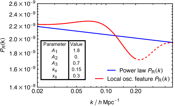
Figure 10: Local oscillatory feature model of the primordial power spectrum (in red) and the power law primordial power spectrum (in blue). The solid red line shows the range of scales covered by the low-$z$ objects and the dashed line the extension provided by the high-$z$ ones. The parameters used to generate this oscillatory feature are given in the table inserted in the figure. The power excess peaks at $k=0.07\text{ h}\text{ Mpc}^{-1}$, reaching a $10\%$ power excess, and is followed by a trough with a minimum power deficit of near $10\%$ at $k=0.20\text{ h}\text{ Mpc}^{-1}$. The model tends to the power law at large scales.

In figure 11 the $P_{g}^{(0)}(k)$ simulations for the local oscillatory feature template are shown. We use the $z=0.9$ bin and the two photometric redshift errors in the low-$z$ reconstructions instead of the previously used $z=0.1$. The sampling variance of this bin is the lowest of all low-$z$ ones at the largest scales, but its shot noise reduces the $S/N$ at the smallest scales, making this choice a conservative one. For the high-$z$ simulations we keep the same favorable bin $z=2.3$ (see figure 2). In all the three cases the simulated $P_{g}^{(0)}(k)$ show the power excess and deficit coming from the primordial feature.

The evidences of the global test appear in figure 12. For all the cases the minimum evidence is for two knots, $N=2$, with values below $10^{-4}$ relative to the highest evidence, which is $N=3$ for the low-$z$ cases and $N=4$ for the high-$z$ one. Significant values of the evidence of $\gtrsim 10\%$ are found at $N=4$ for low-$z$ reconstructions, and at $N=5,6$ for high-$z$ ones. We obtain a threshold of feature detection for deviations of $\approx 2\%$ with substantial evidence when combining all the redshift bins for either low-$z$ or high-$z$.

The reconstructions for the oscillatory feature are shown in figure 13. Low-$z$ reconstructions follow the shape of an $N=3$ curve, i.e., with a change of slope (as expected from the evidences) accounting for both the power excess and deficit at the smallest scales. Their $1-\beta$ values above $0.95$ at different scale ranges indicate that the detected feature is compatible with being sourced by the oscillatory feature template. The case with higher $\delta_{z}$ (top right panel of figure 13) shows less precise distinction between the $N=2$ and the marginalized reconstructions, as their confidence contours have a larger overlap than for the low $\delta_{z}$ scenario. The $1-\beta$ values are consequently smaller, specially at large scales. Nevertheless, at the smallest scales the $1-\beta$ values exceed the $0.95$ threshold that allows us to claim the detection of the feature. In the high-$z$ reconstructions, the contours follow an $N=4$ shape mainly (i.e., with two changes of slope), accounting for a complete oscillation and leading to a decisive detection. The hypothesis test also provides clear detection since there are three scale ranges where $1-\beta>0.95$, being $1-\beta>0.6$ at the largest scales (see the last two columns of table 2).

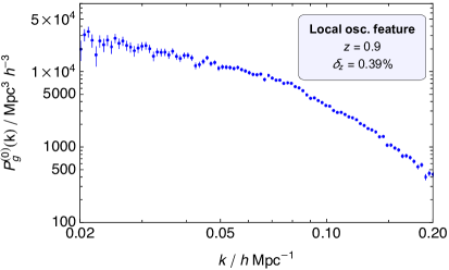
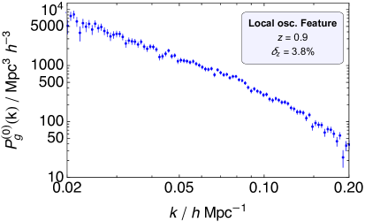
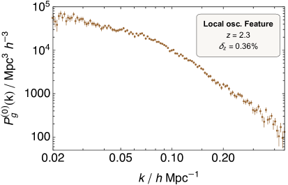
Figure 11: Simulated monopole galaxy power spectrum $P_{g}^{(0)}(k)$ performed for the local oscillatory feature template. Top panels: low-$z$ with low-$\delta_{z}$ (left) and high-$\delta_{z}$ (right). Bottom panel: high-$z$ redshift bin simulation.

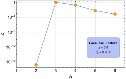
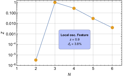
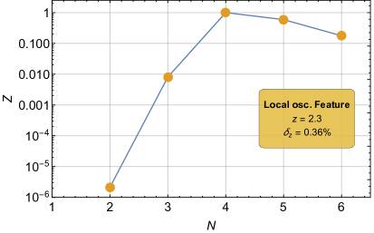
Figure 12: Evidence $Z$ of the oscillatory feature reconstructions for each of the $N$ knots configuration considered for the low-$z$ low-$\delta_{z}$ (top left), low-$z$ high-$\delta_{z}$ (top right) and high-$z$ (bottom) cases.

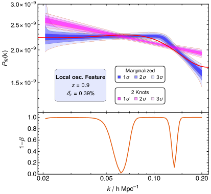
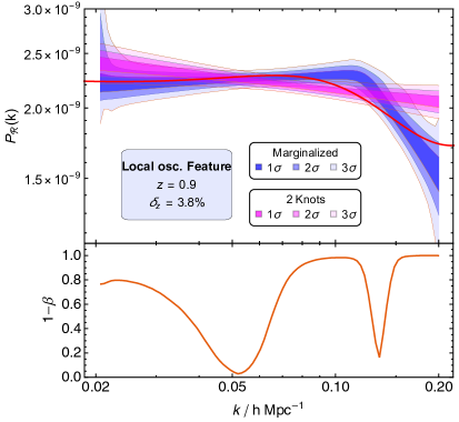
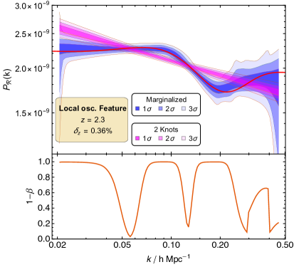
Figure 13: Contours of $P_{\mathcal{R}}(k)$ reconstructions for the oscillatory feature simulations for the $N=2$ case (magenta) and for the case of marginalized probability over $N$ knots (blue). The oscillatory feature template of the primordial power spectrum is shown as a red line. In the bottom panel of each figure the values of the power $1-\beta$ obtained from the hypothesis test are plotted. Top figures: low-$z$ with low-$\delta_{z}$ (left) and high-$\delta_{z}$ (right) reconstructions. Bottom figure: high-$z$ reconstructions.

4.4 Global oscillatory feature

We have tested our methodology with the power law and the bump and oscillatory feature templates, which are local features that approach the power law at large scales. We now consider a different type of feature in $P_{\mathcal{R}}(k)$ which is global, i.e. $P_{\mathcal{R}}(k)$ deviates from the power law at all scales in the form of oscillations. This kind of feature was motivated by a better fit to the Planck data [113, 114], although a modulation is usually required. In those works the oscillations are located at scales from $k\approx 0.04\text{ h}\text{ Mpc}^{-1}$ to $k\approx 0.4\text{ h}\text{ Mpc}^{-1}$, where lensing is significant. The oscillations help to alleviate cosmological tensions, such as those in $H_{0}$, $\sigma_{8}$ or the lensing amplitude $A_{l}$. These global oscillations in the primordial power spectrum are predicted by inflation models with non-Bunch-Davies initial conditions [19, 20, 21] or with axion monodromy [22].

The model used is oscillatory in log-log scale and provides global oscillations for the range of scales that we use ($k\sim 0.01-0.1\text{ h}\text{ Mpc}^{-1}$). It is parametrized including a modulation in the power law primordial power spectrum $P_{\mathcal{R}}^{\text{SM}}$:

$$\mathcal{P}_{\mathcal{R}}(k)=\mathcal{P}_{\mathcal{R}}^{\text{SM}}(k)\left[1+A_{\text{log}}\text{Cos}\left(\omega_{\text{log}}\text{Log}\left({\frac{k}{k_{0}}}\right)+\phi_{\text{log}}\right)\right],$$ (4.1)

where $A_{\text{log}}$, $\omega_{\text{log}}$ and $\phi_{\text{log}}$ are the amplitude, frequency and phase of the oscillations, respectively. Figure 14 shows this modified primordial spectrum template, with the parameters used for our specific feature listed in a table inside.

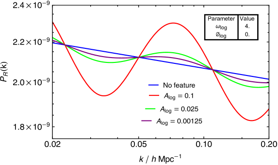
Figure 14: Global oscillatory feature template of eq. 4.1 used as primordial power spectrum for three different values of its amplitude parameter $A_{\text{log}}$: 0.1 (red), 0.02 (green) and 0.01 (purple), corresponding to $10\%$, $3\%$ and $1.5\%$ power deviations. Their frequency $\omega_{\text{log}}$ and phase $\phi_{\text{log}}$ are kept fixed at the values indicated in the inner table. The power law primordial power spectrum is represented in blue. Note the bump peaking near $k=0.07\text{ h}\text{ Mpc}^{-1}$ and the two deficits of power at scales $k\approx 0.035\text{ h}\text{ Mpc}^{-1}$ and $k\approx 0.15\text{ h}\text{ Mpc}^{-1}$.

The simulated $P_{g}^{(0)}(k)$ for the global oscillatory template are shown in figure 15. We study this feature with three different values of its amplitude $A_{\text{log}}$: 0.1, 0.02 and 0.01. Note how the oscillations appear across multiple scale ranges on $P_{g}^{(0)}(k)$.

We reconstructed the primordial power spectrum $P_{\mathcal{R}}(k)$ for the $z=0.9$ bin only in the case of $A_{\text{log}}=0.1$, a conservative redshift bin as explained in the previous section. Then, we use the combination of the five different redshift bins of the low-$z$ simulations for the three amplitudes. Figure 16 shows their global tests. For the $A_{\text{log}}=0.1$ and $A_{\text{log}}=0.02$ cases, $N=6$ has the highest evidence, with negligible contributions from the other number of knots configurations, including $N=2$. This indicates a decisive evidence for feature detection in the reconstructions corresponding to these two amplitudes. For the $A_{\text{log}}=0.01$ feature, $N=3$ has the largest contribution, but $Z_{2}\approx 0.7Z_{3}$, yielding an inconclusive result on the global test. Table 3 summarizes the results of the global test for all the global oscillatory feature cases.

Figure 17 shows the corresponding $P_{\mathcal{R}}(k)$ reconstructions. Both $A_{\text{log}}=0.1$ reconstructions (top panels) show that the marginalized ones deviate strongly from the power law according to the global oscillatory template, as expected from the global test. The hypothesis test indicate values of $1-\beta$ very close to $1$ in those ranges of $k$ where the oscillations are located.

Combining all redshifts (top right panel) the reconstruction is more precise, and it reproduces the last oscillation better than with just one redshift bin. The bottom panels show the reconstructions for the smallest amplitudes $A_{\text{log}}=0.02,0.01$. Note that for these weaker oscillations, the marginalized reconstruction deviates less from the $N=2$ reconstruction, resulting in lower powers of the hypothesis test. While for $A_{\text{log}}=0.02$ $1-\beta>0.95$ in two wide scale ranges, for $A_{\text{log}}=0.01$ $1-\beta<0.65$ at all scales, providing only a ‘hint’ of feature detection according to our threshold.

Table 3 summarizes all the results of the global and local test applied to this feature template. The global oscillatory feature studied can be clearly detected with our methodology for the low-$z$ scenario in both global and local tests, constituting a unambiguous feature detection. The reconstruction power is improved by using the information of all the redshift bins instead of only one. For power deviations of the $3\%$ we detect the feature decisively, and for $2\%$ deviations, substantially. With $A_{\text{log}}=0.01$ (corresponding to 1.5% power deviations) we obtain inconclusive results, so the $2\%$ is the smallest power deviation detected with this feature.

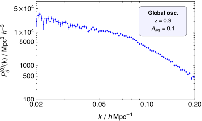
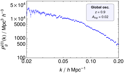
Figure 15: Simulated monopole galaxy power spectrum $P_{g}^{(0)}(k)$ performed for the global oscillatory feature template. The low-$z$ and low $\delta_{z}$ is used in all cases in order to have less sampling variance. Top panels: amplitude of the feature $A_{\text{log}}=0.1$ (left) and $A_{\text{log}}=0.02$ (right). Bottom panel: $A_{\text{log}}=0.01$.

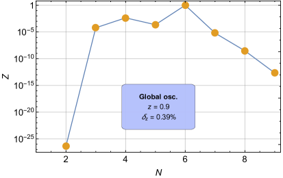
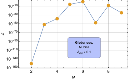
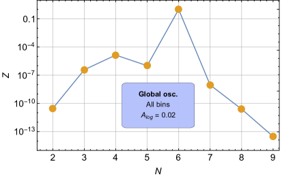
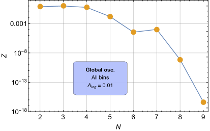
Figure 16: Evidence $Z$ of the global oscillatory template reconstructions for each of the $N$ knots configurations considered in the low-$z$ low-$\delta_{z}$ catalogue. Top panels: evidences for the reconstruction with $A_{\text{log}}=0.1$ with a single bin $z=0.9$ (left) and with all the low-$z$ redshift bins (right). Bottom panels: evidences of the reconstructions using all the low-$z$ redshift bins with $A_{\text{log}}=0.02$ (left) and $A_{\text{log}}=0.01$ (right).

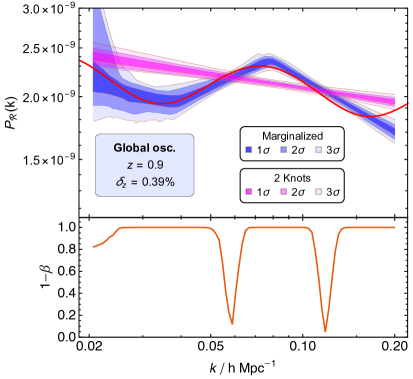
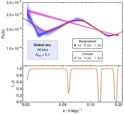
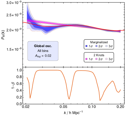
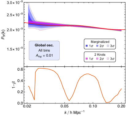
Figure 17: Contours of the $P_{\mathcal{R}}(k)$ reconstructions of the global oscillatory feature template with the low-$z$ low-$\delta_{z}$ catalogue specifications for the $N=2$ case (magenta) and for the case of marginalized probability over $N$ knots (blue). The oscillatory feature template is shown as a red line. In the bottom panel of each figure the value of the power $1-\beta$ used for detecting features in the hypothesis test. Top figures: reconstructions with $A_{\text{log}}=0.1$ for the redshift bin $z=0.9$ (left) and for all the redshift bins (right). Bottom figures: reconstructions for all the redshift bins with $A_{\text{log}}=0.02$ (left) and $A_{\text{log}}=0.01$ (right).

4.5 Summary of the results

The smallest power deviations that we are able to detect with substantial evidence, according to the Jeffreys criterion, are $\approx 2\%$ for all the considered features combining either low or high $z$ redshift bins. In table 2 and table 3 we summarize the detection status for the considered local and global features respectively, based on the global and local tests results, in scenarios with different redshift bins and photometric errors. As shown in these tables, our methodology performed as expected for the reconstructions of the SM $P_{\mathcal{R}}(k)$. For the local bump feature no detection can be claimed, except when combining all the redshift bins of the high-$z$ objects. In this case we detect features with decisive evidence, as we do for all local and global oscillatory realizations with deviations larger than $2\%$.

Local feature	Standard Model		Bump		Oscillation
Test	Global	Local	Global	Local	Global	Local
Low $z$ low $\delta_{z}$	Negative	None	Negative	None	Decisive	Detection
Low $z$ high $\delta_{z}$	Negative	None	Negative	None	Decisive	Detection
High $z$ bin $z=0.9$	Negative	None	Negative	None	Decisive	Detection
High $z$ all bins	—	—	Decisive	Detection	—	—

Table 2: Feature detection status of the SM power law, local bump feature and local oscillatory feature templates of $P_{\mathcal{R}}(k)$ for four different scenarios of low/high redshifts $z$ and low/high photometric errors $\delta_{z}$. The status is classified according to the global and local tests applied, which are based on the evidence comparison and the hypothesis test power respectively. We classify the global test results according to the Jeffreys criterion. For the hypothesis test we claim ‘none’ detection when the power of the test $1-\beta<0.5$ for all scales, ‘hint’ of detection when at least at one scale $0.5<1-\beta<0.95$ and ‘detection’ when at any scale $1-\beta>0.95$.

Global feature	$A_{\text{log}}=0.1$		$A_{\text{log}}=0.02$		$A_{\text{log}}=0.01$
Test	Global	Local	Global	Local	Global	Local
Low $z$ bin $z=0.9$	Decisive	Detection	—	—	—	—
Low $z$ all bins	Decisive	Detection	Decisive	Detection	Inconclusive	Hint

Table 3: Feature detection status of the global oscillatory feature template of $P_{\mathcal{R}}(k)$ with three different amplitudes: $A_{\text{log}}=0.1$, $A_{\text{log}}=0.02$ and $A_{\text{log}}=0.01$, corresponding to $10\%$, $3\%$ and $1.5\%$ power deviations. The status of the feature detection is classified with both global and local indicators as in table 2. The smallest power deviation detected with this feature is 2%, with a substantial status.

5 Application to real data: SDSS LRG 04

5.1 The SDSS LRG 04 data

We present a first application of our methodology to real LSS data. We choose the catalogue provided by the Sloan Digital Sky Survey Luminous Red Galaxies 04 data release (SDSS LRG 04). The catalogue [85] contains a sample of 58360 luminous red galaxies, selected from the 4th data release of the SDSS [115]. These galaxies have a redshift range of $0.155<z<0.474$, and they form a particularly clean and uniform galaxy sample, consisting of luminous early-types galaxies at all redshifts.

Two improvements in the construction of the galaxy power spectrum model for the SDSS LRG 04 are introduced compared to our previous simulations model used in section 3. Its galaxy power spectrum model incorporates a BAO modelling and a semi-empirical description of non-linearities:

$$P_{g}^{(0)}(k)=b^{2}\frac{1+Q_{nl}k^{2}}{1+A_{g}k}P_{\text{dewiggled}}(k),$$ (5.1)

where $b=1.89$ is the galaxy bias and $Q_{nl}$ and $A_{g}$ are parameters accounting for non-linearities [116, 117]. Non-linearities are introduced in a semi-empirical way through the factor $\frac{1+Q_{nl}k^{2}}{1+A_{g}k}$. According to eq. 5.1, $P_{\text{dewiggled}}(k)$ accounts for the BAO signal, written as:

$$P_{\text{dewiggled}}=W_{\text{SDSS}}(k)P_{m}(k)+[1-W_{\text{SDSS}}(k)]P_{\text{nowiggle}}(k),$$ (5.2)

where the matter power spectrum is calculated with CAMB, and $P_{\text{nowiggle}}(k)$ is the ‘no-wiggle’ power spectrum defined in [118], suppressing oscillations of $P_{m}(k)$. $W_{\text{SDSS}}(k)$ is a window function chosen as:

$$W_{\text{SDSS}}(k)\equiv e^{-\left(k/k_{*}\right)^{2}/2},$$ (5.3)

with $k_{*}$ being the wiggle suppression scale defined in [119]. This BAO modelling mimics the smoothing of the power spectrum caused by the non-linear matter clustering.

The analysis of the SDSS LRG 04 data relies on a likelihood function that assumes a cosmology independent and diagonal covariance matrix. The covariance matrix is derived from simulations [85].

Figure 18 shows $P_{m}(k)$, $P_{\text{nowiggle}}(k)$, $P_{\text{dewiggled}}(k)$ and $P_{g}(k)$ along with the SDSS LRG 04 data, ensuring that the constructed $P_{g}(k)$ reproduces the best fit in [85].

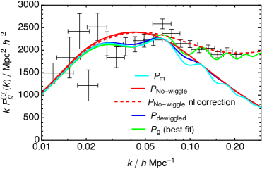
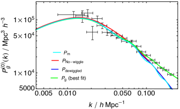
Figure 18: Galaxy power spectrum data for the SDSS LRG 04 (black points) in semi-logarithmic scale represented as $kP_{g}^{(0)}(k)$ (left panel) and logarithmic scale (right panel). In green the employed best fit of $P_{g}^{(0)}(k)$ is plotted, in cyan the matter power spectrum $P_{m}(k)$, in red $P_{\text{nowiggle}}(k)$, and in blue $P_{\text{dewiggled}}(k)$. The uncertainties on $P_{g}^{(0)}(k)$, indicated by the vertical bars, are 1$\sigma$ and they are uncorrelated, even though the horizontal error bars overlap [85]. Note that the models without the non-linear correction $\frac{1+Q_{nl}k^{2}}{1+A_{g}k}$ are not able to properly track the non-linearity of data at scales bigger than $k\approx 0.09$ h/Mpc. In the left panel the effect of the non-linear correction is shown explicitly with two plots of the no wiggle spectrum $P_{\text{nowiggle}}(k)$: without the non-linear correction (continuous red line) and with it (dashed red line).

The linear matter power spectrum provides a reasonably good parametrization of the shape of the monopole galaxy power spectrum at large scales. At small scales $k\sim 0.1$ linear theory fails to fit the data accurately, as shown in the left panel of figure 18. The non-linearities alter the broad shape of the matter power spectrum and wash out baryon wiggles on small scales, among other effects. In particular, most of the departure from the linear regime at the small scales is caused by considering the underlying matter power spectrum given by the multiple galaxies sharing the same dark matter halo instead of the one given by the dark matter halos themselves (see [116] for more details).

In the case of SDSS LRG 04, the non-linear effects start to be significant at $k\approx 0.09$ h/Mpc (see figure 18). The addition of the BAO modelling and the non-linear correction term $\frac{1+Q_{nl}k^{2}}{1+A_{g}k}$ helps significantly in fitting the data [85], although the non-linear correction has a semi-empirical origin and it is not physically derived. More realistic and physically motivated models of galaxy clustering are needed for upcoming stage IV LSS catalogues, including a bias model such as in [104], a model of redshift space distortions as in [94], and a more physically motivated derivation on non-linearities as in [87].

5.2 Results and statistical interpretation

Figure 19 shows the evidences for the SDSS LRG 04. The power law model has the highest evidence $Z$. $Z_{3}$ contributes slightly over a 10% relative to $Z_{2}$, while the evidences for configurations with higher number of knots decrease quasi-exponentially. The $N=1$ configuration, which corresponds to a primordial power spectrum with $n_{s}=1$, has an evidence many orders of magnitude smaller that $Z_{2}$, $Z_{1}\approx 10^{-9}Z_{2}$, as shown in the right panel of figure 19. Thus, it is strongly disfavoured. The Jeffreys criterion favours the power law in our SDSS LRG 04 analysis.

The marginalized probability over $N$ and $N=2$ reconstructions are very similar (top panel of figure 20), except for the 3$\sigma$ confidence level contours of the marginalized one that are much wider, mainly at the largest scales. The hypothesis test does not show significant discriminating power between both distributions at any scale, being $1-\beta<0.08$ at all scales (see bottom panel of figure 20), well below the 0.5 threshold. Therefore, we conclude that deviations are not significant and the power law is the preferred model for the SDSS LRG 04 $P_{\mathcal{R}}(k)$ reconstructions according to both of our tests.

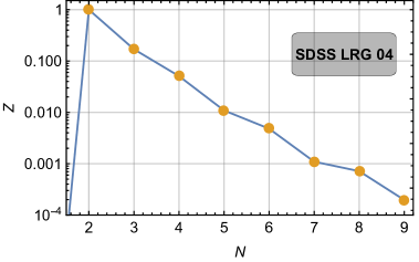
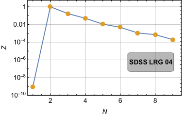
Figure 19: Evidence $Z$ of the SDSS LRG 04 reconstruction for each of the $N$ knots configuration considered. Left panel: all $N$ configurations excluding $N=1$. Right panel: all configurations with $N=1$ case included.

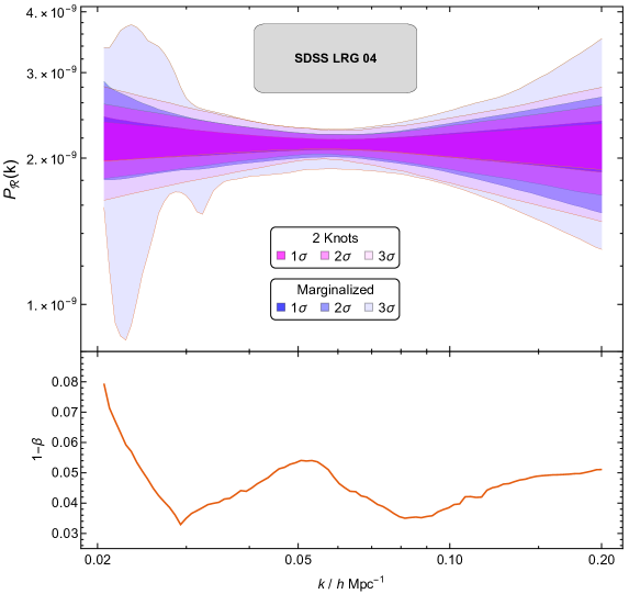
Figure 20: Contours of $P_{\mathcal{R}}(k)$ reconstructions for the SDSS LRG 04 catalogue for the $N=2$ case (magenta) and for the case of marginalized probability over $N$ knots (blue). In the bottom panel the values of the power $1-\beta$ obtained from the hypothesis test are plotted.

6 Conclusions

We have presented a flexible methodology that reconstructs the primordial power spectrum $P_{\mathcal{R}}(k)$ in a model independent way using Bayesian inference. The main advantages of our methodology are that it reconstructs $P_{\mathcal{R}}(k)$ in a non-parametric way, without assuming any specific model. This is done by sampling an arbitrary number $N$ of knots without prior scale binning, which allows a quantitative comparison of different reconstructions based on the evidence $Z$. Models with lower $Z$ are penalized, contributing less to the marginalized probability over $N$ of the $P_{\mathcal{R}}(k)$ reconstructions.

This methodology is applied to detect deviations from the Standard Model primordial power spectrum. For this, we use a global indicator (evidence comparison) and a local test (hypothesis test), as they provide complementary information. The global test compares the overall fit of different $N$ knot models and determines the preferred number of knots. The local test examines each scale separately and identifies where deviations from the power law model ($N=2$) occur. The combination of different redshift bins can also help to detect features as it increases the $S/N$.

We have tested this methodology with simulated spectra, for which the methodology shows a good performance. In the case of simulations with a power law $P_{\mathcal{R}}(k)$, no feature is detected in any of the considered scenarios: low-$z$ objects with both low and high photometric errors $\delta_{z}$ and high-$z$ objects. The reconstructions are sensitive to the $S/N$ of the different catalogues, improving its precision when $S/N$ increases.

In addition, we apply our methodology on different feature templates for $P_{\mathcal{R}}(k)$: a local template for which we generate bump (figure 6) and oscillatory (figure 10) features, and a global oscillatory feature (figure 14). We detected features in all the considered cases, with a sensitivity of $2\%$ power deviations for both global and local features when combining either low-$z$ or high-$z$ redshift bins. For simulations of the local bump, we detected clear deviations from the power law only at high-$z$ and with the combination of all redshift bins. For simulations of a local oscillation, or with global oscillations of 10% or even 3% power deviations, we detected and reconstructed the features convincingly.

In our first application to real data, we used a semi-empirical description of non-linearities and a BAO modelling to reconstruct $P_{\mathcal{R}}(k)$ from the SDSS LRG 04 catalogue (figure 18). The evidence substantially supports the power law model over higher $N>2$ knots configurations, and the local test shows no significant deviations at any scale.

The next step is to apply this methodology to more recent galaxy surveys, incorporating non-linear perturbative effects, BAO modelling and more advanced redshift-space distortions models, such as BOSS [120] [87] and the forthcoming J-PAS [43], DESI [44] and Euclid catalogues [45].

Finally, we can envisage several extensions of this methodology that will be addressed in the near future: the use of higher order splines to interpolate between knots, allowing smoother reconstructions; the inclusion of higher order multipoles, $\ell>0$, of the galaxy power spectrum in the reconstruction, such as the quadrupole or the hexadecapole; the incorporation of weak lensing data and its modelling, which complements the clustering information and allows smaller scales to be explored; and the extension of the methodology to include CMB data in addition to the LSS ones.

7 Appendix

7.1 A) Solution of the label switching problem

The label switching problem appears in Bayesian analysis of models with multiple indistinguishable parameters whose order is arbitrary. The permutation of any of these parameters is equivalent [121], leading to highly multimodal posterior distributions in models with many such parameters.

As described in section 2.1, we sample $N-2$ coordinates for the normalized scales $x_{i}$, with $2\leq i\leq N-1$ (in the case of one or two knots, no $k$ coordinates are sampled). The variables $x_{i}$ are indistinguishable parameters that the sampler can order arbitrarily, causing the label switching problem. A change of coordinates of these scales $x_{i}$ into a $(N-2)$-dimensional hypertriangle of coordinates $x_{i}^{\prime}$ solves the problem [121]:

$$x_{i}^{\prime}=x_{i-1}^{\prime}+\left(1-x_{i-1}^{\prime}\right)\left[1-\left(1-x_{i}\right)^{\frac{1}{N+1-i}}\right],$$ (7.1)

with $x^{\prime}_{1}=x_{1}=0$ and $x^{\prime}_{N}=x_{N}=1$. This transformation can be interpreted as an ordering of the $k$s for sampling, removing the degeneracy of $\mathcal{L}$ with respect to its different $k$ permutations and thus avoiding this problem.

7.2 B) Sample selection in CosmoChord

In this paper, we use the MCMC method CosmoChord to sample the primordial power spectrum. At each step of the sampling, a set of parameters determining the power spectrum is obtained. The MCMC chains represent samples of the primordial power spectrum with a probability according to the posterior. In this method, the likelihood $\mathcal{L}$ increases monotonically as the sampling progresses (see left panel of figure 21). CosmoChord provides the importance weights $\omega$ [80], that once normalized can be interpreted as the probability of that particular point of the parameter space. These weights increase with time $N_{0}$ until they reach a maximum value, then they drop by a few orders of magnitude (see right panel of figure figure 21). Thus, the reconstructions with the highest $\omega$ won’t have the highest $\mathcal{L}$ values. However, they correspond to the tail where $\mathcal{L}$ is barely improved at each step.

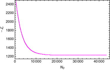
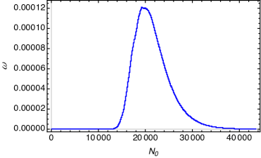
Figure 21: Left panel: minus likelihood $-\mathcal{L}$ against time $N_{0}$. Note how $\mathcal{L}$ increases monotonically with the advance of the step. Right panel: normalized importance weights $\omega$ against $N_{0}$. Note that the maximum in the weights is found at steps when the Markov chain is halfway completed, i.e at $N_{0}\approx N_{0,\text{max}}/2$.

We filter the $i$ obtained reconstructions for each number of knots $N$ to remove the burn-in and to exclude reconstructions with a low likelihood value. For that, we use a Monte Carlo method that selects reconstructions according to their values of $\omega_{i,N}$. If $\omega_{i,N}$ is larger than a random value from 0 to 1, that reconstruction is kept. Otherwise, it is discarded. Due to the shape of importance weights through the chain step $\omega(N_{0})$ (the highest $\mathcal{L}$ points do not have the largest $\omega$, see the correspondence in figure 21), the reconstructions with the highest likelihood also fail this Monte Carlo filtering in most cases, and the ones with the lowest likelihood fail in almost all cases. The retained reconstructions $P_{\mathcal{R}}(k)$ have high $\omega$ values while still having high enough $\mathcal{L}$ values. We label by $P_{\mathcal{R},j,N}$ the reconstructions that passed through this filter.

7.3 C) Local feature template

The parametrization of the primordial power spectrum used as the local bump and local oscillatory feature template has a localized oscillatory burst [15]. Steps in the warp or potential, over which the inflaton rolls in much less than an e-fold, generate oscillations in the power spectrum that can be modelled with this parametrization [15]. It is written as a perturbation of the standard power law $P_{\mathcal{R}}(k)$:

$$\text{Log}\left(\mathcal{P}_{\mathcal{R}}(k)\right)=\exp\left[\text{Log}\mathcal{P}_{\mathcal{R}}^{\text{SM}}(k)+\mathcal{I}_{0}(k)+\text{Log}\left(1+\mathcal{I}_{1}^{2}(k)\right)\right],$$ (7.2)

where the first and second order terms $\mathcal{I}_{0}(k)$ and $\mathcal{I}_{1}(k)$ are:

$$\mathcal{I}_{0}={\left[\mathcal{A}_{1}\mathcal{W}_{1}^{(0)}\left(k/k_{\mathrm{s}}\right)+\mathcal{A}_{2}\mathcal{W}_{2}^{(0)}\left(k/k_{\mathrm{s}}\right)\right.}\\ \left.+\mathcal{A}_{3}\mathcal{W}_{3}^{(0)}\left(k/k_{\mathrm{s}}\right)\right]\mathcal{D}\left(\frac{k/k_{\mathrm{s}}}{x_{\mathrm{s}}}\right),$$ (7.3)

$$\mathcal{I}_{1}=\frac{1}{\sqrt{2}}\left\{\frac{\pi}{2}\left(1-n_{\mathrm{s}}\right)+\left[\mathcal{A}_{1}\mathcal{W}_{1}^{(1)}\left(k/k_{\mathrm{s}}\right)+\mathcal{A}_{2}\mathcal{W}_{2}^{(1)}\left(k/k_{\mathrm{s}}\right)+\mathcal{A}_{3}\mathcal{W}_{3}^{(1)}\left(k/k_{\mathrm{s}}\right)\right]\mathcal{D}\left(\frac{k/k_{\mathrm{s}}}{x_{\mathrm{s}}}\right)\right\},$$ (7.4)

with $\mathcal{D}(x)$ being the dumping function, $\mathcal{D}(x)=\frac{x}{\sinh x}$.

This model has five parameters: three amplitudes $\{\mathcal{A}_{1},\mathcal{A}_{2},\mathcal{A}_{3}\}$, the scale $k_{s}$ where the oscillations start, and the damping parameter $x_{s}$. The set of window functions $W_{i}^{(j)}$ are given below.

The burst in $\mathcal{P}_{\mathcal{R}}(k)$ corresponds to a sudden step-like feature in the inflation potential [25] or the sound speed [26, 27]. Specifically, this parametrization describes a $\tanh$-step in the inflationary potential and in the warp term of a DBI model [15].

The window functions used in the modified power spectrum model of eq. 7.2 are:

$$W_{1}^{(0)}(x)=\frac{1}{2x^{3}}\left[\left(18x-6x^{3}\right)\cos 2x+\left(15x^{2}-9\right)\sin 2x\right],$$ (7.5)

$$\mathcal{W}_{2}^{(0)}(x)=\frac{3}{2x^{3}}\left[\sin(2x)-2x\cos(2x)-x^{2}\sin(2x)\right],$$ (7.6)

$$\mathcal{W}_{3}^{(0)}(x)=\frac{1}{x^{3}}\left[6x\cos(2x)+\left(4x^{2}-3\right)\sin(2x)\right],$$ (7.7)

$$W_{1}^{(1)}(x)=-\frac{1}{x^{3}}\left\{3(x\cos x-\sin x)\left[3x\cos x+\left(2x^{2}-3\right)\sin x\right]\right\},$$ (7.8)

$$W_{2}^{(1)}(x)=\frac{3}{x^{3}}(\sin x-x\cos x)^{2},$$ (7.9)

$$\mathcal{W}_{3}^{(1)}(x)=-\frac{1}{x^{3}}\left[3+2x^{2}-\left(3-4x^{2}\right)\cos(2x)-6x\sin(2x)\right].$$ (7.10)

References

- [1] Planck Collaboration, N. Aghanim, Y. Akrami, M. Ashdown, J. Aumont, C. Baccigalupi et al., Planck 2018 results. VI. Cosmological parameters, A&A 641 (2020) A6 [1807.06209].
- [2] A. H. Guth, Inflationary universe: A possible solution to the horizon and flatness problems, Phys. Rev. D 23 (1981) 347.
- [3] A. Linde, A new inflationary universe scenario: A possible solution of the horizon, flatness, homogeneity, isotropy and primordial monopole problems, Physics Letters B 108 (1982) 389.
- [4] R. Brout, F. Englert and E. Gunzig, The creation of the universe as a quantum phenomenon, Annals of Physics 115 (1978) 78.
- [5] A. Starobinsky, A new type of isotropic cosmological models without singularity, Physics Letters B 91 (1980) 99.
- [6] A. Albrecht and P. J. Steinhardt, Cosmology for grand unified theories with radiatively induced symmetry breaking, Phys. Rev. Lett. 48 (1982) 1220.
- [7] A. Linde, Chaotic inflation, Physics Letters B 129 (1983) 177.
- [8] A. A. Starobinskiǐ, Spectrum of relict gravitational radiation and the early state of the universe, Soviet Journal of Experimental and Theoretical Physics Letters 30 (1979) 682.
- [9] A. D. Linde, A new inflationary universe scenario: A possible solution of the horizon, flatness, homogeneity, isotropy and primordial monopole problems, Physics Letters B 108 (1982) 389.
- [10] F. Bezrukov and M. Shaposhnikov, The Standard Model Higgs boson as the inflaton, Physics Letters B 659 (2008) 703 [0710.3755].
- [11] A. A. Starobinsky, Spectrum of adiabatic perturbations in the universe when there are singularities in the inflation potential, JETP Lett. 55 (1992) 489.
- [12] D. Chowdhury, J. Martin, C. Ringeval and V. Vennin, Assessing the scientific status of inflation after Planck, Phys. Rev. D 100 (2019) 083537 [1902.03951].
- [13] J. Martin, C. Ringeval and V. Vennin, Encyclopædia Inflationaris, Physics of the Dark Universe 5 (2014) 75 [1303.3787].
- [14] G. Tasinato, Analytic approach to non-slow-roll inflation, Phys. Rev. D 103 (2021) 023535 [2012.02518].
- [15] V. Miranda and W. Hu, Inflationary steps in the Planck data, Phys. Rev. D 89 (2014) 083529 [1312.0946].
- [16] P. D. Meerburg, D. N. Spergel and B. D. Wandelt, Searching for oscillations in the primordial power spectrum. II. Constraints from Planck data, Phys. Rev. D 89 (2014) 063537 [1308.3705].
- [17] X. Chen, M. H. Namjoo and Y. Wang, Models of the Primordial Standard Clock, J. Cosmology Astropart. Phys. 02 (2015) 027 [1411.2349].
- [18] K. Kumazaki, S. Yokoyama and N. Sugiyama, Fine Features in the Primordial Power Spectrum, J. Cosmology Astropart. Phys. 12 (2011) 008 [1105.2398].
- [19] J. Martin and R. H. Brandenberger, Trans-Planckian problem of inflationary cosmology, Phys. Rev. D 63 (2001) 123501 [hep-th/0005209].
- [20] J. Martin and R. Brandenberger, Dependence of the spectra of fluctuations in inflationary cosmology on trans-Planckian physics, Phys. Rev. D 68 (2003) 063513 [hep-th/0305161].
- [21] V. Bozza, M. Giovannini and G. Veneziano, Cosmological perturbations from a new physics hypersurface, J. Cosmology Astropart. Phys. 05 (2003) 001 [hep-th/0302184].
- [22] R. Flauger, L. McAllister, E. Silverstein and A. Westphal, Drifting Oscillations in Axion Monodromy, J. Cosmology Astropart. Phys. 10 (2017) 055 [1412.1814].
- [23] P. D. Meerburg, D. N. Spergel and B. D. Wandelt, Searching for oscillations in the primordial power spectrum. II. Constraints from Planck data, Phys. Rev. D 89 (2014) 063537 [1308.3705].
- [24] M. G. Jackson and G. Shiu, Study of the consistency relation for single-field inflation with power spectrum oscillations, Phys. Rev. D 88 (2013) 123511 [1303.4973].
- [25] J. Adams, B. Cresswell and R. Easther, Inflationary perturbations from a potential with a step, Phys. Rev. D 64 (2001) 123514 [astro-ph/0102236].
- [26] A. Achucarro, J.-O. Gong, S. Hardeman, G. A. Palma and S. P. Patil, Features of heavy physics in the CMB power spectrum, J. Cosmology Astropart. Phys. 01 (2011) 030 [1010.3693].
- [27] G. Cañas-Herrera, J. Torrado and A. Achúcarro, Bayesian reconstruction of the inflaton’s speed of sound using CMB data, Phys. Rev. D 103 (2021) 123531 [2012.04640].
- [28] C. R. Contaldi, M. Peloso, L. Kofman and A. D. Linde, Suppressing the lower multipoles in the CMB anisotropies, J. Cosmology Astropart. Phys. 07 (2003) 002 [astro-ph/0303636].
- [29] R. Sinha and T. Souradeep, Post-WMAP assessment of infrared cutoff in the primordial spectrum from inflation, Phys. Rev. D 74 (2006) 043518 [astro-ph/0511808].
- [30] U. H. Danielsson, Note on inflation and trans-Planckian physics, Phys. Rev. D 66 (2002) 023511 [hep-th/0203198].
- [31] X. Chen, Primordial Features as Evidence for Inflation, J. Cosmology Astropart. Phys. 01 (2012) 038 [1104.1323].
- [32] C. L. Bennett, R. S. Hill, G. Hinshaw, D. Larson, K. M. Smith, J. Dunkley et al., Seven-year Wilkinson Microwave Anisotropy Probe (WMAP) Observations: Are There Cosmic Microwave Background Anomalies?, ApJS 192 (2011) 17 [1001.4758].
- [33] Planck Collaboration, Y. Akrami, M. Ashdown, J. Aumont, C. Baccigalupi, M. Ballardini et al., Planck 2018 results. VII. Isotropy and statistics of the CMB, A&A 641 (2020) A7 [1906.02552].
- [34] C. J. Copi, D. Huterer, D. J. Schwarz and G. D. Starkman, Lack of large-angle TT correlations persists in WMAP and Planck, MNRAS 451 (2015) 2978 [1310.3831].
- [35] C. Monteserín, R. B. Barreiro, P. Vielva, E. Martínez-González, M. P. Hobson and A. N. Lasenby, A low cosmic microwave background variance in the Wilkinson Microwave Anisotropy Probe data, MNRAS 387 (2008) 209 [0706.4289].
- [36] M. Cruz, P. Vielva, E. Martínez-González and R. B. Barreiro, Anomalous variance in the WMAP data and Galactic foreground residuals, MNRAS 412 (2011) 2383 [1005.1264].
- [37] D. J. Schwarz, C. J. Copi, D. Huterer and G. D. Starkman, CMB anomalies after Planck, Classical and Quantum Gravity 33 (2016) 184001 [1510.07929].
- [38] F. Paci, A. Gruppuso, F. Finelli, A. De Rosa, N. Mandolesi and P. Natoli, Hemispherical power asymmetries in the WMAP 7-year low-resolution temperature and polarization maps, MNRAS 434 (2013) 3071 [1301.5195].
- [39] Y. Akrami, Y. Fantaye, A. Shafieloo, H. K. Eriksen, F. K. Hansen, A. J. Banday et al., Power Asymmetry in WMAP and Planck Temperature Sky Maps as Measured by a Local Variance Estimator, ApJ 784 (2014) L42 [1402.0870].
- [40] Planck Collaboration, P. A. R. Ade, N. Aghanim, M. Arnaud, M. Ashdown, J. Aumont et al., Planck 2015 results. XIII. Cosmological parameters, A&A 594 (2016) A13 [1502.01589].
- [41] P. Vielva, E. Martínez-González, R. B. Barreiro, J. L. Sanz and L. Cayón, Detection of Non-Gaussianity in the Wilkinson Microwave Anisotropy Probe First-Year Data Using Spherical Wavelets, ApJ 609 (2004) 22 [astro-ph/0310273].
- [42] M. Cruz, E. Martínez-González, P. Vielva and L. Cayón, Detection of a non-Gaussian spot in WMAP, MNRAS 356 (2005) 29 [astro-ph/0405341].
- [43] N. Benitez, R. Dupke, M. Moles, L. Sodre, J. Cenarro, A. Marin-Franch et al., J-PAS: The Javalambre-Physics of the Accelerated Universe Astrophysical Survey, arXiv e-prints (2014) arXiv:1403.5237 [1403.5237].
- [44] DESI Collaboration, A. Aghamousa, J. Aguilar, S. Ahlen, S. Alam, L. E. Allen et al., The DESI Experiment Part I: Science,Targeting, and Survey Design, arXiv e-prints (2016) arXiv:1611.00036 [1611.00036].
- [45] R. Laureijs, J. Amiaux, S. Arduini, J. L. Auguères, J. Brinchmann, R. Cole et al., Euclid Definition Study Report, arXiv e-prints (2011) arXiv:1110.3193 [1110.3193].
- [46] S. L. Bridle, A. M. Lewis, J. Weller and G. Efstathiou, Reconstructing the primordial power spectrum, MNRAS 342 (2003) L72 [astro-ph/0302306].
- [47] J. Simon, L. Verde and R. Jimenez, Constraints on the redshift dependence of the dark energy potential, Phys. Rev. D 71 (2005) 123001 [astro-ph/0412269].
- [48] M. Bridges, A. N. Lasenby and M. P. Hobson, A Bayesian analysis of the primordial power spectrum, MNRAS 369 (2006) 1123 [astro-ph/0511573].
- [49] R. Sinha and T. Souradeep, Post-WMAP assessment of infrared cutoff in the primordial spectrum from inflation, Phys. Rev. D 74 (2006) 043518 [astro-ph/0511808].
- [50] L. Covi, J. Hamann, A. Melchiorri, A. Slosar and I. Sorbera, Inflation and WMAP three year data: Features are still present, Phys. Rev. D 74 (2006) 083509 [astro-ph/0606452].
- [51] M. Bridges, A. N. Lasenby and M. P. Hobson, WMAP 3-yr primordial power spectrum, MNRAS 381 (2007) 68 [astro-ph/0607404].
- [52] M. Joy, A. Shafieloo, V. Sahni and A. A. Starobinsky, Is a step in the primordial spectral index favored by CMB data ?, J. Cosmology Astropart. Phys. 06 (2009) 028 [0807.3334].
- [53] P. Paykari and A. H. Jaffe, Optimal Binning of the Primordial Power Spectrum, ApJ 711 (2010) 1 [0902.4399].
- [54] K. Ichiki, R. Nagata and J. Yokoyama, Cosmic discordance: Detection of a modulation in the primordial fluctuation spectrum, Phys. Rev. D 81 (2010) 083010 [0911.5108].
- [55] Z.-K. Guo, D. J. Schwarz and Y.-Z. Zhang, Reconstruction of the primordial power spectrum from CMB data, J. Cosmology Astropart. Phys. 08 (2011) 031 [1105.5916].
- [56] G. Goswami and J. Prasad, Maximum entropy deconvolution of primordial power spectrum, Phys. Rev. D 88 (2013) 023522 [1303.4747].
- [57] Planck Collaboration, Y. Akrami, F. Arroja, M. Ashdown, J. Aumont, C. Baccigalupi et al., Planck 2018 results. X. Constraints on inflation, A&A 641 (2020) A10.
- [58] Planck Collaboration, P. A. R. Ade, N. Aghanim, C. Armitage-Caplan, M. Arnaud, M. Ashdown et al., Planck 2013 results. XXII. Constraints on inflation, A&A 571 (2014) A22 [1303.5082].
- [59] Planck Collaboration, P. A. R. Ade, N. Aghanim, M. Arnaud, F. Arroja, M. Ashdown et al., Planck 2015 results. XX. Constraints on inflation, A&A 594 (2016) A20 [1502.02114].
- [60] S. Hannestad, Reconstructing the primordial power spectrum - A New algorithm, J. Cosmology Astropart. Phys. 04 (2004) 002 [astro-ph/0311491].
- [61] G. Brando and E. V. Linder, Exploring early and late cosmology with next generation surveys, Phys. Rev. D 101 (2020) 103510 [2001.07738].
- [62] P. Mukherjee and Y. Wang, Direct Wavelet Expansion of the Primordial Power Spectrum, ApJ 598 (2003) 779 [astro-ph/0301562].
- [63] P. Mukherjee and Y. Wang, Primordial power spectrum reconstruction, J. Cosmology Astropart. Phys. 12 (2005) 007 [astro-ph/0502136].
- [64] A. Ravenni, L. Verde and A. J. Cuesta, Red, Straight, no bends: primordial power spectrum reconstruction from CMB and large-scale structure, J. Cosmology Astropart. Phys. 08 (2016) 028 [1605.06637].
- [65] C. Sealfon, L. Verde and R. Jimenez, Smoothing spline primordial power spectrum reconstruction, Phys. Rev. D 72 (2005) 103520 [astro-ph/0506707].
- [66] L. Verde and H. V. Peiris, On Minimally-Parametric Primordial Power Spectrum Reconstruction and the Evidence for a Red Tilt, J. Cosmology Astropart. Phys. 07 (2008) 009 [0802.1219].
- [67] S. Dorn, E. Ramirez, K. E. Kunze, S. Hofmann and T. A. Ensslin, Generic inference of inflation models by non-Gaussianity and primordial power spectrum reconstruction, J. Cosmology Astropart. Phys. 06 (2014) 048 [1403.5067].
- [68] J. A. Vázquez, M. Bridges, M. P. Hobson and A. N. Lasenby, Model selection applied to reconstruction of the Primordial Power Spectrum, J. Cosmology Astropart. Phys. 06 (2012) 006 [1203.1252].
- [69] W. J. Handley, A. N. Lasenby, H. V. Peiris and M. P. Hobson, Bayesian inflationary reconstructions from 2018 data, Phys. Rev. D 100 (2019) 103511 [1908.00906].
- [70] G. Aslanyan, L. C. Price, K. N. Abazajian and R. Easther, The Knotted Sky I: Planck constraints on the primordial power spectrum, J. Cosmology Astropart. Phys. 08 (2014) 052 [1403.5849].
- [71] C. Gauthier and M. Bucher, Reconstructing the primordial power spectrum from the CMB, J. Cosmology Astropart. Phys. 10 (2012) 050 [1209.2147].
- [72] M. S. Esmaeilian, M. Farhang and S. Khodabakhshi, Detectable Data-driven Features in the Primordial Scalar Power Spectrum, ApJ 912 (2021) 104 [2011.14774].
- [73] P. Paykari, F. Lanusse, J. L. Starck, F. Sureau and J. Bobin, PRISM: Sparse recovery of the primordial power spectrum, A&A 566 (2014) A77 [1402.1983].
- [74] K. Ichiki and R. Nagata, Brute force reconstruction of the primordial fluctuation spectrum from five-year Wilkinson Microwave Anisotropy Probe observations, Phys. Rev. D 80 (2009) 083002.
- [75] A. Lasenby and C. Doran, Closed universes, de Sitter space, and inflation, Phys. Rev. D 71 (2005) 063502 [astro-ph/0307311].
- [76] J. Chluba, J. Hamann and S. P. Patil, Features and new physical scales in primordial observables: Theory and observation, International Journal of Modern Physics D 24 (2015) 1530023 [1505.01834].
- [77] W. Handley, “CosmoChord: Planck 2018 update.” https://zenodo.org/record/3370086, Aug., 2019.
- [78] A. Lewis and S. Bridle, Cosmological parameters from CMB and other data: A Monte Carlo approach, Phys. Rev. D 66 (2002) 103511 [astro-ph/0205436].
- [79] W. J. Handley, M. P. Hobson and A. N. Lasenby, polychord: nested sampling for cosmology., MNRAS 450 (2015) L61 [1502.01856].
- [80] W. J. Handley, M. P. Hobson and A. N. Lasenby, POLYCHORD: next-generation nested sampling, MNRAS 453 (2015) 4384 [1506.00171].
- [81] B. Xu and L.-X. Xia, Reconstructing the evolution of deceleration parameter with the non-parametric Bayesian method, Ap&SS 365 (2020) 44.
- [82] R. Trotta, Applications of Bayesian model selection to cosmological parameters, MNRAS 378 (2007) 72.
- [83] H. Jeffreys, The Theory of Probability, Oxford Classic Texts in the Physical Sciences. Oxford University Press, 1998.
- [84] G. Cowan, Statistical data analysis. Oxford University Press, 1998.
- [85] M. Tegmark, D. J. Eisenstein, M. A. Strauss, D. H. Weinberg, M. R. Blanton, J. A. Frieman et al., Cosmological constraints from the SDSS luminous red galaxies, Phys. Rev. D 74 (2006) 123507 [astro-ph/0608632].
- [86] S. Casas, J. Lesgourgues, N. Schöneberg, M. Sabarish V., L. Rathmann, M. Doerenkamp et al., Euclid: Validation of the MontePython forecasting tools, arXiv e-prints (2023) arXiv:2303.09451 [2303.09451].
- [87] H. Gil-Marín, W. J. Percival, J. R. Brownstein, C.-H. Chuang, J. N. Grieb, S. Ho et al., The clustering of galaxies in the SDSS-III Baryon Oscillation Spectroscopic Survey: RSD measurement from the LOS-dependent power spectrum of DR12 BOSS galaxies, MNRAS 460 (2016) 4188 [1509.06386].
- [88] S. Brieden, H. Gil-Marín and L. Verde, Model-agnostic interpretation of 10 billion years of cosmic evolution traced by BOSS and eBOSS data, J. Cosmology Astropart. Phys. 08 (2022) 024 [2204.11868].
- [89] W. J. Percival, D. Burkey, A. Heavens, A. Taylor, S. Cole, J. A. Peacock et al., The 2dF Galaxy Redshift Survey: spherical harmonics analysis of fluctuations in the final catalogue, MNRAS 353 (2004) 1201 [astro-ph/0406513].
- [90] C. Alcock and B. Paczynski, An evolution free test for non-zero cosmological constant, Nature 281 (1979) 358.
- [91] F. Beutler, S. Saito, H.-J. Seo, J. Brinkmann, K. S. Dawson, D. J. Eisenstein et al., The clustering of galaxies in the SDSS-III Baryon Oscillation Spectroscopic Survey: testing gravity with redshift space distortions using the power spectrum multipoles, MNRAS 443 (2014) 1065 [1312.4611].
- [92] N. Kaiser, Clustering in real space and in redshift space, MNRAS 227 (1987) 1.
- [93] R. Scoccimarro, Redshift-space distortions, pairwise velocities, and nonlinearities, Phys. Rev. D 70 (2004) 083007 [astro-ph/0407214].
- [94] A. Taruya, T. Nishimichi and S. Saito, Baryon acoustic oscillations in 2d: Modeling redshift-space power spectrum from perturbation theory, Phys. Rev. D 82 (2010) 063522.
- [95] T. Nishimichi and A. Taruya, Baryon acoustic oscillations in 2d. ii. redshift-space halo clustering in -body simulations, Phys. Rev. D 84 (2011) 043526.
- [96] S. Bonoli, A. Marí n-Franch, J. Varela, H. V. Ramió, L. R. Abramo, A. J. Cenarro et al., The miniJPAS survey: A preview of the universe in 56 colors, A&A 653 (2021) A31.
- [97] C. Queiroz et al., The miniJPAS survey quasar selection – I. Mock catalogues for classification, MNRAS 520 (2023) 3476 [2202.00103].
- [98] C. Queiroz et al., “In preparation.” (2023).
- [99] J. N. Fry, The Evolution of Bias, ApJ 461 (1996) L65.
- [100] M. Aparicio Resco, A. L. Maroto, J. S. Alcaniz, L. R. Abramo, C. Hernández-Monteagudo, N. Benítez et al., J-PAS: forecasts on dark energy and modified gravity theories, MNRAS 493 (2020) 3616 [1910.02694].
- [101] S. M. Croom, B. J. Boyle, T. Shanks, R. J. Smith, L. Miller, P. J. Outram et al., The 2dF QSO Redshift Survey - XIV. Structure and evolution from the two-point correlation function, MNRAS 356 (2005) 415 [astro-ph/0409314].
- [102] N. P. Ross, Y. Shen, M. A. Strauss, D. E. Vanden Berk, A. J. Connolly, G. T. Richards et al., Clustering of Low-redshift (z 2.2) Quasars from the Sloan Digital Sky Survey, ApJ 697 (2009) 1634 [0903.3230].
- [103] A. G. Sánchez and S. Cole, The galaxy power spectrum: precision cosmology from large-scale structure?, MNRAS 385 (2008) 830 [0708.1517].
- [104] P. McDonald and A. Roy, Clustering of dark matter tracers: generalizing bias for the coming era of precision LSS, J. Cosmology Astropart. Phys. 08 (2009) 020 [0902.0991].
- [105] F. Beutler, S. Saito, H.-J. Seo, J. Brinkmann, K. S. Dawson, D. J. Eisenstein et al., The clustering of galaxies in the SDSS-III Baryon Oscillation Spectroscopic Survey: testing gravity with redshift space distortions using the power spectrum multipoles, MNRAS 443 (2014) 1065 [1312.4611].
- [106] H. Gil-Marín, J. Noreña, L. Verde, W. J. Percival, C. Wagner, M. Manera et al., The power spectrum and bispectrum of SDSS DR11 BOSS galaxies - I. Bias and gravity, MNRAS 451 (2015) 539 [1407.5668].
- [107] H.-J. Seo and D. J. Eisenstein, Improved Forecasts for the Baryon Acoustic Oscillations and Cosmological Distance Scale, ApJ 665 (2007) 14 [astro-ph/0701079].
- [108] Collaboration, N. Aghanim, Y. Akrami, M. Ashdown, J. Aumont, C. Baccigalupi et al., 2018 results. VI. Cosmological parameters, A&A 641 (2020) A6 [1807.06209].
- [109] A. Lewis, A. Challinor and A. Lasenby, Efficient Computation of Cosmic Microwave Background Anisotropies in Closed Friedmann-Robertson-Walker Models, ApJ 538 (2000) 473 [astro-ph/9911177].
- [110] M. Davis and P. J. E. Peebles, A survey of galaxy redshifts. V. The two-point position and velocity correlations., ApJ 267 (1983) 465.
- [111] N. Kaiser, Clustering in real space and in redshift space, MNRAS 227 (1987) 1.
- [112] J. Carron, M. Wolk and I. Szapudi, On the information content of the matter power spectrum, MNRAS 453 (2015) 450 [1412.5511].
- [113] D. K. Hazra, A. Antony and A. Shafieloo, One spectrum to cure them all: signature from early Universe solves major anomalies and tensions in cosmology, J. Cosmology Astropart. Phys. 08 (2022) 063 [2201.12000].
- [114] A. Antony, F. Finelli, D. K. Hazra and A. Shafieloo, Discordances in Cosmology and the Violation of Slow-Roll Inflationary Dynamics, Phys. Rev. Lett. 130 (2023) 111001 [2202.14028].
- [115] J. K. Adelman-McCarthy, M. A. Agüeros, S. S. Allam, K. S. J. Anderson, S. F. Anderson, J. Annis et al., The Fourth Data Release of the Sloan Digital Sky Survey, ApJS 162 (2006) 38 [astro-ph/0507711].
- [116] S. Cole, W. J. Percival, J. A. Peacock, P. Norberg, C. M. Baugh, C. S. Frenk et al., The 2dF Galaxy Redshift Survey: power-spectrum analysis of the final data set and cosmological implications, MNRAS 362 (2005) 505 [astro-ph/0501174].
- [117] U. Seljak, A. Slosar and P. McDonald, Cosmological parameters from combining the Lyman-alpha forest with CMB, galaxy clustering and SN constraints, J. Cosmology Astropart. Phys. 10 (2006) 014 [astro-ph/0604335].
- [118] D. J. Eisenstein and W. Hu, Power Spectra for Cold Dark Matter and Its Variants, ApJ 511 (1999) 5 [astro-ph/9710252].
- [119] D. J. Eisenstein, H.-J. Seo and M. White, On the Robustness of the Acoustic Scale in the Low-Redshift Clustering of Matter, ApJ 664 (2007) 660 [astro-ph/0604361].
- [120] D. J. Eisenstein, D. H. Weinberg, E. Agol, H. Aihara, C. Allende Prieto, S. F. Anderson et al., SDSS-III: Massive Spectroscopic Surveys of the Distant Universe, the Milky Way, and Extra-Solar Planetary Systems, AJ 142 (2011) 72 [1101.1529].
- [121] R. Buscicchio, E. Roebber, J. M. Goldstein and C. J. Moore, Label switching problem in Bayesian analysis for gravitational wave astronomy, Phys. Rev. D 100 (2019) 084041 [1907.11631].