Validity of Markovian modeling for transient memory-dependent epidemic dynamics

Abstract

The initial transient phase of an emerging epidemic is of critical importance for data-driven model building, model-based prediction of the epidemic trend, and articulation of control/prevention strategies. In principle, quantitative models for real-world epidemics need to be memory-dependent or non-Markovian, but this presents difficulties for data collection, parameter estimation, computation and analyses. In contrast, the difficulties do not arise in the traditional Markovian models. To uncover the conditions under which Markovian and non-Markovian models are equivalent for transient epidemic dynamics is outstanding and of significant current interest. We develop a comprehensive computational and analytic framework to establish that the transient-state equivalence holds when the average generation time matches and average removal time, resulting in minimal Markovian estimation errors in the basic reproduction number, epidemic forecasting, and evaluation of control strategy. Strikingly, the errors depend on the generation-to-removal time ratio but not on the specific values and distributions of these times, and this universality will further facilitate estimation rectification. Overall, our study provides a general criterion for modeling memory-dependent processes using the Markovian frameworks.

Introduction

When an epidemic emerges, the initial transient phase of the disease spreading dynamics before a steady state is reached is of paramount importance, for two reasons [1, 2, 3, 4, 5, 6, 7, 8, 9, 10, 11, 12, 13, 14]. First, key indicators or parameters characterizing the underlying dynamical process and critical for prediction and articulation of control strategies, such as the generation time, the serial intervals and the basic reproduction number, are required to be estimated when the dynamics have not reached a steady state. Second, it is during the transient phase control and mitigation strategies can be effectively applied for preventing a large scale outbreak. Prediction and control depend, of course, on a quantitative model of the epidemic process, which can be constructed based on the key parameters estimated from data collected during the transient phase. In principle, since the dynamical processes underlying real-world epidemics are generally memory-dependent in the sense that the state evolution depends on the history, a rigorous modeling framework needs to be of the non-Markovian type, but this presents great challenges in terms of data collection, parameter estimation, computation and analyses [15, 16, 17]. The difficulties can be significantly alleviated by adopting the traditional memoryless, Markovian framework  [18, 19, 20, 21, 22, 23, 24, 25, 26, 27, 28, 29]. An outstanding question is, under what conditions will an approximate equivalence between non-Markovian and Markovian dynamics hold during the transient phase of the epidemic? Additionally, another important issue remains, how are the errors of Markovian estimation determined? The purpose of this paper is to a comprehensive answer to these questions.

The COVID-19 pandemic has highlighted the need and importance of understanding disease spreading and transmission to accurately predict, control and manage future outbreaks through non-pharmacological interventions and vaccine allocation strategies [1, 2, 3, 4, 5, 6, 7, 8, 9, 10, 11]. To accomplish these goals, accurate mathematical modeling of the disease spreading dynamics is key. In a general population, epidemic transmission occurs via some kind of point process, where individuals become infected at different points in time. It has been known that point processes in the real world are typically non-Markovian with a memory effect in which the distribution of the interevent times is not exponential [3, 30, 31, 32, 33, 34, 35, 36, 37, 38, 39, 26, 40, 41, 42, 43, 44, 45, 46, 47]. For example, the interevent time distribution arising from the virus transmission with COVID-19 is not of the memoryless exponential type but typically exhibits memory-dependent features characterized by the Weibull distribution [3]. Strictly speaking, from a modeling perspective, disease spreading should be described by a non-Markovian process. A non-Markovian approach takes into account historical memory of disease progression, mathematically resulting in a complex set of integro-differential equations in the form of convolution.

There are significant difficulties with non-Markovian modeling of memory-dependent disease spreading. The foremost is data availability. In particular, while standard epidemic spreading models are available, the model parameters need to be estimated through data. A non-Markovian model often requires detailed and granular data that can be difficult to get, especially during the early stage of the epidemic where accurate modeling is most needed [15]. From a theoretical point of view, it is desired to obtain certain closed-form solutions for key quantities such as the onset and size of the epidemic outbreak, but this is generally impossible for non-Markovian models [18, 48]. Computationally, accommodating memory effects in principle makes the underlying dynamical system infinitely dimensional, practically requiring solving an unusually large number of dynamical variables through a large number of complex integro-differential equations [16, 17]. In contrast, in an idealized Markovian point process, events occur at a fixed rate, leading to an exponential distribution for the interevent time intervals and consequently a memoryless process. If the spreading dynamics were of the Markovian type, the aforementioned difficulties associated with non-Markovian dynamics no longer exist. In particular, a Markovian spreading process can be described by a small number of ordinary differential equations with a few parameters that can be estimated even from sparse data, and the numerical simulations can be carried out in a computationally extremely efficient manner [18, 19, 20, 21, 22, 23, 24, 25, 26, 27, 28, 29]. For these reasons, many recent studies of the COVID-19 pandemic assumed Markovian behaviors to avoid or “escape” from the difficulties associated with non-Markovian modeling [4, 5, 6, 7, 8, 9, 10, 11]. The issue is whether such a simplified approach can be justified. Addressing this issue requires a comprehensive understanding of the extent to which the Markovian approach represents a good approximation to model non-Markovian type of memory-dependent spreading dynamics, and specifically of the conditions under which the Markovian theory can produce accurate results that match those from the non-Markovian model.

There were previous studies of the so-called steady-state equivalence between Markovian and non-Markovian modeling for epidemic spreading. In particular, when the system has reached a steady state, such an equivalence can be established through a modified definition of the effective infection rate [24, 25, 21]. From a realistic point of view, the equivalence limited only to steady states may not be critical as the transient phase of the spreading process before any steady state is reached is more relevant and significant. For example, when an epidemic occurs, it is of fundamental interest to estimate the key indicators such as the generation time (the time interval between the infections of the infector and infectee in a transmission chain), the serial interval (the time from illness onset in the primary case to illness onset in the secondary case), and the basic reproduction number (the average number of secondary transmissions from one infected person), but they are often needed to be estimated when the dynamics have not reached a steady state [12, 13, 14, 3, 4, 5, 6, 7, 8, 9, 10, 11]. It is the equivalence in the transient dynamics rather than the steady state that determines whether the transmission features in the early stages of a memory-dependent disease outbreak can be properly measured through Markovian modeling. Moreover, it is only during the transient phase control and mitigation strategies can be effective for preventing a large scale outbreak. Discovering when and how a non-Markovian process can be approximated by a Markovian process during the transient state is thus of paramount importance. To our knowledge, such a “transient-state equivalence”, where the Markovian and non-Markovian transmission models produce similar behaviors over the entire transient transmission period, has not been established. In fact, the conditions under which the transient equivalence may hold are completely unknown at the present.

In this paper, we present results from a comprehensive study of how memory effects impact the Markovian estimations in terms of the errors that arise from the Markovian hypothesis. We consider both the steady-state and transient-state equivalences between non-Markovian and Markovian models. We first rigorously show that, in the steady state, a memory-dependent non-Markovian spreading process is always equivalent to certain Markovian (memoryless) ones. We then turn to the transient states and find that an approximate equivalence can still be achieved but only if the average generation time matches the average removal time in the memory-dependent non-Markovian spreading dynamics. Qualitatively, the equality of the two times gives rise to a memoryless correlation between the infection and removal processes, thereby minimizing the impact of any memory effects. We establish that the equality gives the condition under which Markovian theory accurately describes memory-dependent transmission.

One fundamental quantity underlying an epidemic process is the basic reproduction number $R_{0}$. Our theoretical analysis indicates that, when the average generation and removal times are equal, the transient-state equivalence between memory-dependent and memoryless transmissions will minimize the error of Markovian approach in estimating $R_{0}$ and lead to its accurate epidemic forecasting and prevention evaluation. Another finding is that the generation-to-removal time ratio plays a decisive role in the accuracy of the Markovian approximation. Specifically, if the average generation time is smaller (greater) than the average removal time, the Markovian approximate will lead to an overestimation (underestimation) of $R_{0}$ and epidemic forecasting as well as the errors of the prevention evaluation, which can also be verified based on readily accessible clinical data of 4 types of real diseases.

Strikingly, the estimation accuracy is largely determined by the time ratio and hardly depends on the particular forms of time distributions or the specific values of the average generation and removal times. This property is of great practical significance, because it is in general challenging to obtain the detailed distributions of the generation and removal times in the early stages of the epidemic [49], but their average values can be reliably estimated even during the transient phase [50, 51, 52, 53, 54]. Moreover, based on this property, we have developed a semi-empirical mathematical relationship that connects the errors in estimating $R_{0}$ with the generation-to-removal time ratio. This relationship holds practical value as it can be utilized to rectify errors in real-world scenarios. And the rectification of $R_{0}$ and epidemic forecasting can be accomplished through our web-based application [55].

Overall, our study establishes a general criterion for modeling memory-dependent processes within the context of Markovian frameworks. Once the condition for the existence of a transient-state equivalence between Markovian and non-Markovian dynamics is fulfilled, epidemic forecasting and prevention evaluation can be carried out using the Markovian model, again based solely on the data collected from the transient phase.

Results

The overall structure of this work is depicted in Fig. 1. The section titled “Model” presents the Model building of the age-stratified Susceptible-Infected-Removed (SIR) spreading (Fig. 1a), highlighting the difference between the Markovian (memoryless) and non-Markovian (memory-dependent) dynamics (Fig. 1b). In the “Dynamical equivalence” section, we demonstrate the equivalence between Markovian (memoryless) and non-Markovian (memory-dependent) dynamics for steady state and transient dynamics, which will further lead to the accurate description of memory-dependent dynamics by the Markovian theory (Fig. 1c). The section “Markovian approximation of memory-dependent spreading dynamics” analyzes the errors of the Markovian approach in estimating $R_{0}$, epidemic forecasting, and prevention evaluation (Fig. 1d).

Model

We articulate an age-stratified SIR spreading dynamics model, in which the entire population is partitioned into various age groups with intricate age-specific contact rates among them. The distribution of population across different age groups is represented by an age distribution vector (p), with the age-dependent contact matrix (A) quantifying the transmission rates between different age groups. Both p and A can be constructed from empirical data [56, 57]. For convenience, to distinguish between the actual dynamical process and its theoretical treatment, throughout this paper we use the terms “memory-dependent” and “memoryless” to describe actual spreading processes and Monte Carlo simulations, while in various theoretical analyses, the corresponding terms are “non-Markovian” and “Markovian.”

The mechanism of disease transmission across different age groups and the recovery or death of infected individuals can be described by the SIR model, as illustrated in Fig. 1a, where the individuals are placed into three compartments: susceptible (S), infected (I), and removed (R). Susceptible individuals (S) have not contracted the disease and are at risk of being infected. Infected individuals (I) have contracted the disease and can infect others. Removed individuals (R) have recovered or died from the disease. There are two dynamical processes: (1) infection during which susceptible individuals become infected by others and transition to the I state so as to become capable of infecting others, as shown in Fig. 1a(i–iii); and (2) removal during which infected individuals recover or die from the disease transmission and transition to the R state, as shown in Fig. 1a(iv). The ability to infect others of an infected individual can be characterized by the infection time distribution, $\psi_{\mathrm{inf}}(\tau)$, where $\tau$ denotes the time elapsed between the time the individual is infected and the current time, and the probability of the infection process occurring during the time interval $[\tau,\tau+d\tau)$ is given by $\psi_{\mathrm{inf}}(\tau)d\tau$, as shown in Fig. 1b(i). Likewise, the removal process is described by the removal time distribution, $\psi_{\mathrm{rem}}(\tau)$, where the probability of a removal occurring within the time interval $[\tau,\tau+d\tau)$ is given by $\psi_{\mathrm{rem}}(\tau)d\tau$, as shown in Fig. 1b(ii). The time distributions of the infection and removal processes with memory effects are general, with the exponential distributions associated with the memoryless process being a special case of the memory-dependent process.

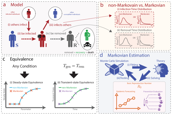
Figure 1: Overall structure of this work. (a) SIR Model. Each individual belongs to one of the three states: susceptible (S), infected (I), or removed (R). When infected (i), a susceptible individual will switch into the I state (ii) and gain the ability to infect others (iii). An infected individual is removed (through recovery or death) with a probability (iv). (b) Non-Markovian versus Markovian process. The infection capacity of an infected individual is characterized by the infection time distribution $\psi_{\mathrm{inf}}(\tau)$ and its removal can be described by the removal time distribution $\psi_{\mathrm{rem}}(\tau)$. For the non-Markovian process, the distributions can assume quite general forms, while the distributions are exponential for a Markovian process. (c) Equivalence between non-Markovian and Markovian processes: (i) steady-state equivalence holds under all conditions; (ii) transient-state equivalence only holds only when $T_{\mathrm{gen}}$ is equal to $T_{\mathrm{rem}}$. (d) Markovian estimation of memory-dependent process. (i) The initial phase of the Monte Carlo simulation is used to fit the parameters according to the Markovian theory. (ii) Important issues such as the estimation of $R_{0}$, epidemic forecasting, and the evaluation of the vaccination strategies can be addressed by the theory. (iii) The remaining data generated by the Monte Carlo simulation is used to test the accuracy of the estimated $R_{0}$, epidemic forecasting, and prevention evaluation.

The generic memory-dependent SIR spreading dynamics can be described by a set of deterministic integro-differential equations:

$$\frac{ds_{l}(t)}{dt} =-s_{l}(t)k\sum_{m=1}^{n}{A_{lm}p_{m}\int_{0}^{t}{\omega_{\mathrm{inf}}(t-t^{\prime})\Psi_{\mathrm{rem}}(t-t^{\prime})dc_{m}(t^{\prime})}},$$ (1)

$$i_{l}(t) =\int_{0}^{t}{\Psi_{\mathrm{rem}}(t-t^{\prime})dc_{l}(t^{\prime})},$$ (2)

$$r_{l}(t) =\int_{0}^{t}{[1-\Psi_{\mathrm{rem}}(t-t^{\prime})]dc_{l}(t^{\prime})},$$ (3)

where $s_{l}(t)$, $i_{l}(t)$, and $r_{l}(t)$, respectively, denote the fractions of the susceptible, infected, and removed individuals in age group $l$. The term $c_{l}(t)=1-s_{l}(t)=i_{l}(t)+r_{l}(t)$ represents the fraction of cumulative infections (including both infections and removals) with respect to the total population in age group $l$, while $k$ is a parameter to adjust the overall contacts and $n$ is the total number of age groups. The quantity $\omega_{\mathrm{inf}}(\tau)$ represents the hazard function of $\psi_{\mathrm{inf}}(\tau)$, meaning the rate at which infection happens at $\tau$, given that the infection has not occurred before $\tau$. $\Psi_{\mathrm{rem}}(\tau)$ is the survival function of $\psi_{\mathrm{rem}}(\tau)$, meaning probability that the removal has not occurred by $\tau$ (see Method for detailed calculations for hazard and survival functions). When the infection and removal time distributions are known, Eqs. (1–3) provide an accurate description of generic (including memory-dependent and memoryless) SIR spreading Monte Carlo simulations in an age-stratified population-based system. As shown in Figs. 2a–c, the theory is validated by the agreement between the numerical solutions of Eqs. (1–3) and the results from direct Monte Carlo simulations. (See Method for a detailed description of the Monte Carlo simulation procedure.)

Eqs. (1–3) provide a general framework encompassing both non-Markovian and Markovian descriptions. If the infection and removal time distributions are exponential: $\psi_{\mathrm{inf}}(\tau)=\gamma e^{-\gamma\tau}$ and $\psi_{\mathrm{rem}}(\tau)=\mu e^{-\mu\tau}$, Eqs. (1–3) can be reformulated into a Markovian theory and further simplified into a set of ordinary differential equations with the constant infection and removal rates $\gamma$ and $\mu$ (A detailed derivation of these equations is presented in Supplementary Note 1) :

$$\frac{ds_{l}(t)}{dt} =-s_{l}(t)k\gamma\sum_{m=1}^{n}{A_{lm}p_{m}i_{m}(t)},$$ (4)

$$\frac{di_{l}(t)}{dt} =s_{l}(t)k\gamma\sum_{m=1}^{n}{A_{lm}p_{m}i_{m}(t)}-\mu i_{l}(t),$$ (5)

$$\frac{dr_{l}(t)}{dt} =\mu i_{l}(t).$$ (6)

While the non-Markovian and Markovian theories [Eqs. (1–3) and Eqs. (4–6), respectively] describe the memory-dependent and memoryless Monte Carlo simulations, we focus on whether the Markovian theory can accurately capture memory-dependent dynamics and how memory effects influence its accuracy. For this purpose, we seek to establish the equivalence between Markovian and non-Markovian approaches for describing spreading dynamics.

Dynamical equivalence

Eqs. (1–6) provide a base to study the steady-state equivalence and transient-state equivalence between non-Markovian and Markovian theories, where a steady state characterizes the long-term dynamics of disease spreading and a transient state is referred to as the short-term behavior prior to system’s having reached the steady state. As illustrated in Fig. 1c, note that steady-state equivalence means that the two types of spreading dynamics attain identical steady states [24, 25, 21], whereas transient-state equivalence implies that two types of dynamics are consistent throughout the entire transmission period. Transient-state equivalence thus implies steady-state equivalence, but not vice versa. Since Eqs. (1–6) also provides a numerical framework for Monte Carlo simulations, the terms “steady-state equivalence” and “transient-state equivalence” not only describe the connection between non-Markovian and Markovian theories, but also illustrate the relationship between memory-dependent and memoryless processes. Therefore, the equivalence between the two theories implies the equivalence between the two corresponding processes, and vice versa.

Steady-state equivalence

Eqs. (1–3) give the following transcendental equation for determining the steady state (see Supplementary None 2 for detailed derivation):

$$\tilde{s}_{l}=\acute{s}_{l}e^{-\frac{R_{0}}{\Lambda_{\mathrm{max}}}\sum_{m=0}^{n}{kA_{lm}p_{m}(\tilde{r}_{m}-\acute{r}_{m})}},$$ (7)

where $\tilde{s}_{l}=\lim\limits_{t\to+\infty}{s_{l}(t)}$ and $\tilde{r}_{l}=\lim\limits_{t\to+\infty}{r_{l}(t)}$ denote the fractions of the susceptible and removed individuals in age group $l$ at the steady state (note that $\tilde{s}_{l}=1-\tilde{r}_{l}$, because at steady state, no infection exists), while $\acute{s}_{l}=s_{l}(0)$ and $\acute{r}_{l}=r_{l}(0)$ represent the initial fractions of the susceptible and removed individuals in this age group. For non-Markovian dynamics, basic reproduction number $R_{0}$ can be determined by:

$$R_{0}=\Lambda_{\mathrm{max}}\int_{0}^{+\infty}{\omega_{\mathrm{inf}}(\tau)\Psi_{\mathrm{rem}}(\tau)d\tau}.$$ (8)

For Markovian dynamics, $R_{0}$ is given by

$$R_{0}=\frac{\gamma\Lambda_{\mathrm{max}}}{\mu}.$$ (9)

where $\Lambda_{\mathrm{max}}$ is the maximum eigenvalue of the matrix $k\textbf{{A}}\circ\textbf{{p}}$, and $\circ$ denotes a row-wise Hadamard product between a matrix and a vector (see Supplementary Note 2 for a detailed description). Since Eq. (7) applies to both non-Markovian and Markovian dynamics, an identical $R_{0}$ value in the two cases will result in equivalent steady states from the same initial conditions. Consequently, for a given non-Markovian spreading process, there exists an infinite number of Markovian models with the same steady state, as the $R_{0}$ value is only determined by the ratio of $\gamma$ to $\mu$, but not by either value.

As shown in Fig. 2d, memory-dependent and memoryless spreading dynamics that reach the same steady state with the identical $R_{0}$ value confirm the steady-state equivalence. Fig. 2e demonstrates that, even for $R_{0}$ ranging from $0.01$ to $2$, the equivalent memory-dependent and memoryless spreading dynamics still produce highly consistent steady states that can be calculated from Eq. (7), which share the same critical point of phase transition at $R_{0}=1$.

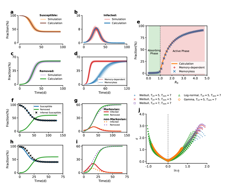
Figure 2: Steady-state and transient-state equivalence between Markovian and non-Markovian dynamics. a–c: The solid brown, blue, and green curves represent the theoretical results of the susceptible, infected, and removed fractions, while the solid orange, red, and purple curves show the corresponding results of 100 independent Monte Carlo simulations. d: The red and blue curves, respectively, depict the removed fractions from the memory-dependent and memoryless Monte Carlo simulations of 100 independent realizations with steady-state equivalence. e: Red $+$ and blue $\times$ markers, respectively, represent the steady-state removed fractions of memory-dependent and memoryless Monte Carlo simulations for different values of $R_{0}$, where each marker is the result of averaging 100 independent simulations. The orange curve is the numerical calculations from Eq. (7), and the vertical dashed line denotes the critical point $R_{0}=1$. f–g: For $T_{\mathrm{gen}}=T_{\mathrm{rem}}$ in the non-Markovian theory: the blue and green curves in f denote the susceptible and removed fractions, while the black $\times$ markers represent the inferred susceptible fractions calculated by substituting removed fractions in Eq. (11), which agrees with the susceptible curve calculated from Eq. (1). The red and blue curves in g denote the non-Markovian susceptible and removed fractions, while the orange and purple dashed curves are the corresponding curves of the Markovian transmission obtained from Eqs. (13–14), which agree with the non-Markovian results. (The Euler-Lotka equation assumes exponential growth of a disease outbreak during the initial stage. As a result, the Markovian curves in g slightly deviate from the non-Markovian ones as the cumulative infections increase.) h–i: For $T_{\mathrm{gen}}\neq T_{\mathrm{rem}}$ in the non-Markovian theory, the inferred susceptible curve does not match the numerical result, and the susceptible and infected curves of the Markovian transmission obtained from Eqs. (13–14) do not match the corresponding non-Markovian results. j: Five scenarios for the non-Markovian time-distribution setting (within each scenario, $T_{\mathrm{inf}}$ and $T_{\mathrm{rem}}$ are fixed): Weibull, $T_{\mathrm{inf}}=5$, $T_{\mathrm{rem}}=7$ (blue $+$); Weibull, $T_{\mathrm{inf}}=5$, $T_{\mathrm{rem}}=5$ (red $\times$); Weibull, $T_{\mathrm{inf}}=7$, $T_{\mathrm{rem}}=7$ (purple $\Box$); log-normal, $T_{\mathrm{inf}}=5$, $T_{\mathrm{rem}}=7$ (green $\triangle$); gamma, $T_{\mathrm{inf}}=5$, $T_{\mathrm{rem}}=7$ (orange $\Diamond$). The value of $T_{\mathrm{gen}}$ is modified to adjust $\ln{\eta}$ for better visualization.

Transient-state equivalence

From the preceding section, we used the basic reproduction number $R_{0}$, a fundamental metric quantifying the number of secondary infections generated by a single individual, to characterize the steady-state equivalence. Here, we propose to quantify the transient-state equivalence through the average generation time $T_{\mathrm{gen}}$ that measures the “velocity” at which secondary infections occur. This time can be calculated as [3, 58],

$$T_{\mathrm{gen}}=\int_{0}^{+\infty}{\tau\psi_{\mathrm{gen}}(\tau)d\tau},$$

where

$$\psi_{\mathrm{gen}}(\tau)=\frac{\omega_{\mathrm{inf}}(\tau)\Psi_{\mathrm{rem}}(\tau)}{\int_{0}^{+\infty}{\omega_{\mathrm{inf}}(\tau^{\prime})\Psi_{\mathrm{rem}}(\tau^{\prime})d\tau^{\prime}}}$$ (10)

is the generation time distribution. Effectively, $T_{\mathrm{gen}}$ measures the average duration of disease transmission from an infected individual to the next generation of individuals. Likewise, the average infection time $T_{\mathrm{inf}}$ and the average removal time $T_{\mathrm{rem}}$ are defined as the mean values of the infection and removal time distributions:

$$T_{\mathrm{inf}} =\int_{0}^{+\infty}{\tau\psi_{\mathrm{inf}}(\tau)d\tau},$$

$$T_{\mathrm{rem}} =\int_{0}^{+\infty}{\tau\psi_{\mathrm{rem}}(\tau)d\tau}.$$

In calculating $T_{\mathrm{gen}}$, the individual’s removal is taken into account, while $T_{\mathrm{inf}}$ measures the average time of the first disease transmission of an infectious individual without factoring in removal. In the classical memoryless transmission with exponential distributions $\psi_{\mathrm{inf}}(\tau)$ and $\psi_{\mathrm{rem}}(\tau)$, the equality $T_{\mathrm{gen}}=T_{\mathrm{rem}}$ holds. However, for memory-dependent spreading, the possible scenarios are: $T_{\mathrm{gen}}=T_{\mathrm{rem}}$, $T_{\mathrm{gen}}<T_{\mathrm{rem}}$, or $T_{\mathrm{gen}}>T_{\mathrm{rem}}$. Specifically, because $T_{\mathrm{gen}}$, $T_{\mathrm{inf}}$ and $T_{\mathrm{rem}}$ all represent the mean values of distributions, it is possible for $T_{\mathrm{rem}}$ to be shorter than $T_{\mathrm{gen}}$ or $T_{\mathrm{inf}}$ in some situations. And our web-based application demonstrates the impact of parameters on the time distributions (infection, removal, and generation) as well as their average times [55].

For a non-Markovian spreading process, if the equality $T_{\mathrm{gen}}=T_{\mathrm{rem}}$ holds, in the transient state we have

$$s_{l}(t)\simeq\acute{s}_{l}e^{-\frac{R_{0}}{\Lambda_{\mathrm{max}}}\sum_{m=0}^{n}{kA_{lm}p_{m}[r_{m}(t)-\acute{r}_{m}]}},$$ (11)

which exhibits a memoryless transmission pattern similar to Markovian dynamics (see Supplementary Notes 3 for a detailed analysis). Intuitively, the equality $T_{\mathrm{gen}}=T_{\mathrm{rem}}$ signifies that the infection and removal processes occur concurrently, which in turn leads to a memoryless relationship between the two processes, thereby minimizing the memory effects. Furthermore, to determine the corresponding Markovian parameters $\gamma$ and $\mu$ of the Markovian transmission which is equivalent to the non-Markovian dynamics in the transient state, we need to utilize the Euler-Lotka equation [59, 58, 50]:

$$1=R_{0}\int_{0}^{+\infty}{e^{-g\tau}\psi_{\mathrm{gen}}(\tau)d\tau},$$ (12)

where $g$ denotes the growth rate of the non-Markovian dynamics and is another measure of how quickly the epidemic is spreading within a population. Therefore, we can calculate the values of the basic reproduction number, $R_{0}$, and growth rate, $g$, in the non-Markovian dynamic by using Eqs. (8), (10) and (12). Additionally, the Markovian form of $\psi_{\mathrm{gen}}(\tau)$ according to Eq. (10) is $\mu e^{-\mu\tau}$, and the equivalent Markovian and non-Markovian dynamics in the transient state have the same values of $R_{0}$ and the equal values of $g$. By substituting $\psi_{\mathrm{gen}}(\tau)=\mu e^{-\mu\tau}$ and the calculated $R_{0}$ and $g$ into Eq. (12), we can determine the value of $\mu$. Furthermore, using Eq. (9), we can find the value of $\gamma$ based on $\mu$. Hence, the Markovian parameters $\gamma$ and $\mu$ are determined as follows:

$$\gamma =\frac{gR_{0}}{\Lambda_{\mathrm{max}}(R_{0}-1)},$$ (13)

$$\mu =\frac{g}{R_{0}-1}.$$ (14)

And we provide visualizations that illustrate how the values of $\gamma$ and $\mu$ are influenced by the distribution parameters in our web-based application[55].

As illustrated in Figs. 2f–g, when the equality $T_{\mathrm{gen}}=T_{\mathrm{rem}}$ holds for the non-Markovian dynamics, Eq. (11) holds, which can be seen by comparing the susceptible curve calculated from Eq. (1) to that inferred from Eq. (11), as shown in Fig. 2f. In this case, the Markovian spreading curves deduced from Eqs. (13–14) closely align with the non-Markovian transient curves, as shown in Fig. 2g. However, as shown in Figs. 2h–i, if the equality does not hold, the equivalence in transient states breaks down. It is important to note that the Euler-Lotka equation assumes an exponential growth of a disease outbreak and is only reasonable at the initial stage. Consequently, as the cumulative infections increase (Fig. 2g), the Markovian curves will exhibit slight deviations from the non-Markovian counterparts. Meanwhile, because the equivalent dynamics share the same $R_{0}$, they will ultimately reach the same steady state, ensuring that deviations will diminish while they approach the steady state.

To evaluate, under different values of the generation-to-removal time ratio $\eta\equiv T_{\mathrm{gen}}/T_{\mathrm{rem}}$ for non-Markovian dynamics we introduce a metric, $\varepsilon$, to quantify the difference from the corresponding Markovian results calculated from Eqs. (13–14) (see Method for detailed definition of $\varepsilon$). Fig. 2j shows, for non-Markovian numerical calculations, five scenarios under various forms of time distributions $\psi_{\mathrm{inf}}(\tau)$ and $\psi_{\mathrm{rem}}(\tau)$ constrained by certain average infection and removal times: Weibull, $T_{\mathrm{inf}}=5$, $T_{\mathrm{rem}}=7$; Weibull, $T_{\mathrm{inf}}=7$, $T_{\mathrm{rem}}=7$; Weibull, $T_{\mathrm{inf}}=5$, $T_{\mathrm{rem}}=5$; log-normal, $T_{\mathrm{inf}}=5$, $T_{\mathrm{rem}}=7$; and gamma, $T_{\mathrm{inf}}=5$, $T_{\mathrm{rem}}=7$ (see Method for detailed definitions of Weibull, log-normal, and gamma distributions). The $T_{\mathrm{gen}}$ value is adjusted to obtain different values of $\ln{\eta}$. For $\ln{\eta}=0$, i.e., $T_{\mathrm{gen}}=T_{\mathrm{rem}}$, the “distance” $\varepsilon$ between the transient states of non-Markovian and Markovian dynamics with parameters determined from Eqs. (13–14) is minimal. Otherwise, $\varepsilon$ increases as $\ln{\eta}$ deviates from zero. Remarkably, Fig. 2j shows that $\varepsilon$ depends only on the ratio of $T_{\mathrm{gen}}$ to $T_{\mathrm{rem}}$, not on the values of $T_{\mathrm{gen}}$, $T_{\mathrm{inf}}$, or $T_{\mathrm{rem}}$, and it is not affected by the specific form of the time distributions.

Furthermore, it is important to note that the condition $T_{\mathrm{gen}}=T_{\mathrm{rem}}$ can guarantee transient-state equivalence between a non-Markovian dynamic and a Markovian one, but according to Eqs. (13–14), it does not imply that the average generation and removal times of the non-Markovian dynamic must be equal to those of the equivalent Markovian one. For instance, if a non-Markovian dynamic satisfies the condition of transient-state equivalence and we keep its average generation and removal times fixed, altering the shape of the corresponding time distributions will change the transmission speed [58]. This change, in turn, affects the infection and removal rates of the equivalent Markovian dynamic, leading to different average generation and removal times for the Markovian equivalent dynamic (see Supplementary 4 and 5 for a detailed analysis).

Markovian approximation of memory-dependent spreading dynamics

As illustrated in Fig. 1d, testing the applicability of Markovian theory for memory-dependent spreading dynamics requires three steps. The first step is fitting, where the memory-dependent Monte Carlo simulation data are divided into two parts: (a) a short initial period used as the training data for fitting the Markovian parameters in Eqs. (4–6), and (b) the remaining testing data for evaluating the performance of the Markovian model (see Methods for details of the fitting procedure). The second step is to use the fitted Markovian model for tasks such as estimating $R_{0}$, predicting outbreaks and assessing the prevention effects of different vaccination strategies. The third step is testing, i.e., evaluating the accuracy of the Markovian model, e.g., by comparing the estimated and actual $R_{0}$ values, disease outbreaks and prevention effects. As real-world disease spreading is subject to environmental, social and political disturbing factors, for the fitting and testing steps, we conduct Monte Carlo simulations of stochastic memory-dependent disease outbreaks to generate the training and testing data.

Here, we first analyze the influence of $\eta$ on the estimation of $R_{0}$ using the Markovian theory, and use the results to design two tasks to evaluate the applicability of the theory in epidemic forecasting and prevention evaluation of memory-dependent spreading. For comparison, we also generate the corresponding results from the non-Markovian theory in the two tasks.

Estimation of basic reproduction number

Estimating basic reproduction number $R_{0}$ is crucial for determining the ultimate prevalence of disease spreading and for assessing the effectiveness of various disease containment measures [59, 58, 50]. When using the Markovian theory to fit the early-stage transmission of a memory-dependent process, a key parameter that can affect the estimation of $R_{0}$ is the ratio $\eta$. To develop an analysis, recall the basic principle for estimating $R_{0}$: disease spreading dynamics can be viewed as a combination of two parallel processes: infection and removal. In particular, the infection process is the reproduction of the disease within each generation, where each infected individual generates an average of $R_{0}$ newly infected individuals in the subsequent generation after a mean time period $T_{\mathrm{gen}}$. In the removal process, infected individuals are removed from the spreading chain, where each generation takes an average time $T_{\mathrm{rem}}$ to be removed. For a Markovian type of dynamics with constant $\gamma$ and $\mu$, the equality $T_{\mathrm{gen}}=T_{\mathrm{rem}}$ holds. Consequently, during the Markovian fitting step, the average number of new infections upon the removal of a single infected individual is taken as the value of $R_{0}$. For memory-dependent spreading, if the equality $T_{\mathrm{gen}}=T_{\mathrm{rem}}$ holds, the memory-dependent spreading curves will possess an approximate memoryless feature so that $R_{0}$ can be still be estimated by counting the number of new infections at the time when the current generation of infections is removed, as shown in Fig. 3a. However, for $T_{\mathrm{gen}}<T_{\mathrm{rem}}$, more than one generation is produced while the current generation is removed, $R_{0}$ estimated by the Markovian theory will represent an overestimate, as shown in Fig. 3b. For $T_{\mathrm{gen}}>T_{\mathrm{rem}}$, less than one generation is created during $T_{\mathrm{rem}}$, the Markovian theory will give an underestimate of $R_{0}$, as shown in Fig. 3c.

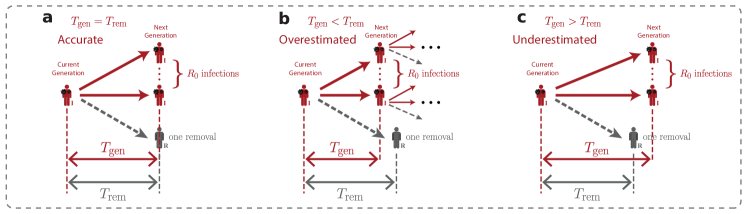
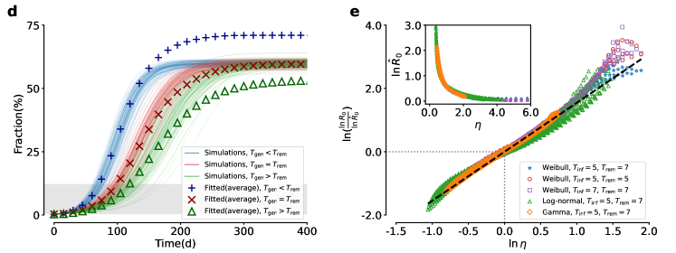
Figure 3: Estimation of $R_{0}$. a–c: Mechanism of the $R_{0}$ estimation. The red arrows represent the infection process of the next generation by the current generation, while the dashed arrows denote the removal of the current generation. The relationship between $T_{\mathrm{gen}}$ and $T_{\mathrm{rem}}$ influences the number of new infections when the current generation of infections is removed. For $T_{\mathrm{gen}}=T_{\mathrm{rem}}$, the number of new infections is exactly $R_{0}$. For $T_{\mathrm{gen}}<T_{\mathrm{rem}}$, the number of new infections is greater than $R_{0}$. For $T_{\mathrm{gen}}>T_{\mathrm{rem}}$, the number of new infections is smaller than $R_{0}$. d: Three distinct categories of disease spreading with the same value of $R_{0}$: $T_{\mathrm{gen}}<T_{\mathrm{rem}}$ (blue curves), $T_{\mathrm{gen}}=T_{\mathrm{rem}}$ (red curves), and $T_{\mathrm{gen}}>T_{\mathrm{rem}}$) (green curves), where the fractions of cumulative infected individuals (i.e., sum of infected and removed fractions) are calculated using 100 independent realizations. The predicted future evolution of the spreading dynamics by the Markovian theory with the fitted parameters are also shown: $T_{\mathrm{gen}}<T_{\mathrm{rem}}$ (blue $+$ symbols), $T_{\mathrm{gen}}=T_{\mathrm{rem}}$ (red $\times$ symbols), and $T_{\mathrm{gen}}>T_{\mathrm{rem}}$ (green $\triangle$ symbols), where the gray area marks the average cumulative infected fraction for selecting the training data (see Method for details). e: The relationship between $\ln{(\ln{R_{0}}/\ln{\hat{R}_{0}})}$ ($R_{0}$ represents the real basic reproduction number, while $\hat{R_{0}}$ denoted the estimated one) and $\ln{\eta}$ where the horizontal and vertical dotted lines show that the equality between $T_{\mathrm{gen}}$ and $T_{\mathrm{rem}}$ results in an accurate estimation of $R_{0}$ and the dashed line represents a linear fitting with the slope $1.55$. Inset: the relation between $\ln\hat{R}_{0}$ and $\eta$ with the asymptotic behaviors: for $\eta\to 0$, $\hat{R}_{0}\to+\infty$ ($\ln{\hat{R}_{0}}\to+\infty$), and for $\eta\to+\infty$, $\hat{R}_{0}\to 1$ ($\ln{\hat{R}_{0}}\to 1$).

Fig. 3d shows fitting curves (training data) from the early stage of memory-dependent spreading simulations that have identical $R_{0}$ values for $T_{\mathrm{gen}}=T_{\mathrm{rem}}$ (red curves), $T_{\mathrm{gen}}<T_{\mathrm{rem}}$ (blue curves), and $T_{\mathrm{gen}}>T_{\mathrm{rem}}$ (green curves) from the Markovian theory. When the equality $T_{\mathrm{gen}}=T_{\mathrm{rem}}$ holds, the Markovian theory with fitted parameters generates accurate the future evolution (red $\times$ symbols). For $T_{\mathrm{gen}}<T_{\mathrm{rem}}$, the outbreak in the initial stage is accelerated, resulting in an overestimation by the Markovian theory (blue $+$ symbols). For $T_{\mathrm{gen}}<T_{\mathrm{rem}}$, the initial outbreaks are decelerated, leading to an underestimation by the Markovian approach (blue $+$ symbols).

The above qualitative insights lead to a semi-empirical relationship between the Markovian-estimated basic reproduction number $\hat{R}_{0}$ and its actual value $R_{0}$ as:

$$\hat{R}_{0}=(R_{0})^{\eta^{-a}},$$ (15)

where $a$ is a positive coefficient (see Method for a detailed derivation). The value of $a$ is a crucial and constant parameter in Eq. (15), and it needs to be determined by fitting it to the data. Once this constant $a$ is obtained, the actual value of $R_{0}$ can be derived by adjusting the estimated $\hat{R}_{0}$ based on Eq. (15), and more accurate steady state can be calculated by using Eq. (7).

Eq. (15) implies the relationship $\ln{(\ln{R_{0}}/\ln{\hat{R}_{0}})}=a\ln{\eta}$. We use the five scenarios specified in Fig. 2j for memory-dependent Monte Carlo simulations. Fig. 3e shows the linear relationship between $\ln{(\ln{R_{0}}/\ln{\hat{R}_{0}})}$ and $\ln{\eta}$, providing support for our qualitative analysis of the Markovian estimation. The estimation of $R_{0}$ also depends on the ratio $\eta$ and is relatively insensitive to the particular forms of the time distributions or the specific values of $T_{\mathrm{gen}}$, $T_{\mathrm{inf}}$, or $T_{\mathrm{rem}}$. The results in the inset of Fig. 3e further confirm that the estimated $\hat{R}_{0}$ approaches one when $T_{\mathrm{gen}}$ is much larger than $T_{\mathrm{rem}}$ and tends to $+\infty$ when $T_{\mathrm{gen}}$ is much smaller than $T_{\mathrm{rem}}$. By fitting the available data, we have determined the value of $a$ to be $1.55$. After obtaining the value of $a$, we can develop our web-based application for rectifying $R_{0}$ and epidemic forecasting [55].

Epidemic forecasting

As suggested in Fig. 1d, we evaluate the efficacy of Markovian theory for epidemic forecasting. We use the initial period of Monte Carlo simulation data to fit parameters under both Markovian and non-Markovian hypotheses and then to predict future disease outbreaks. The remaining simulation data are leveraged to evaluate the accuracy of the Markovian and non-Markovian forecasting results. Regardless of the type of time distributions in the memory-dependent Monte Carlo simulations (Weibull, log-normal, or gamma), the non-Markovian model fits the training data in a consistent manner, i.e., by selecting Weibull time distribution.

Figs. 4a–c show the evolution of the spreading dynamics from three types of memory-dependent Monte Carlo simulations with Weibull infection and removal distributions, where the shape parameters $\alpha_{\mathrm{inf}}$ and $\alpha_{\mathrm{rem}}$ are selected according to $\ln{\alpha_{\mathrm{inf}}}=-0.3,\ln{\alpha_{\mathrm{rem}}}=1.2$ (Fig. 4a), $\ln{\alpha_{\mathrm{inf}}}=0.45,\ln{\alpha_{\mathrm{rem}}}=0.45$ (Fig. 4b), and $\ln{\alpha_{\mathrm{inf}}}=1.2,\ln{\alpha_{\mathrm{rem}}}=-0.3$ (Fig. 4c), for $T_{\mathrm{inf}}=5$ and $T_{\mathrm{rem}}=7$. For the Weibull distributions, we have $\alpha_{\mathrm{inf}}<\alpha_{\mathrm{rem}}$, $\alpha_{\mathrm{inf}}=\alpha_{\mathrm{rem}}$ and $\alpha_{\mathrm{inf}}>\alpha_{\mathrm{rem}}$, corresponding to $T_{\mathrm{gen}}<T_{\mathrm{rem}}$, $T_{\mathrm{gen}}=T_{\mathrm{rem}}$, and $T_{\mathrm{gen}}>T_{\mathrm{rem}}$, respectively. We compare the simulated cumulative infected fractions to those predicted by the Markovian and non-Markovian theories. In general, the non-Markovian theory provides more accurate predictions than the Markovian theory. For the specific parameter setting $\ln{\alpha_{\mathrm{inf}}}=0.45,\ln{\alpha_{\mathrm{rem}}}=0.45$ (i.e., $T_{\mathrm{gen}}=T_{\mathrm{rem}}$), both theories yield a high accuracy.

The accuracy can be assessed through the forecasting error $\varepsilon^{+}$ that evaluates whether a theory overestimates or underestimates the steady-state cumulative infection, i.e., quantifying the extent of deviation between the results obtained from Markovian or non-Markovian theories and those derived from Monte Carlo simulations (see Method for detailed definition of $\varepsilon^{+}$). A plus value of $\varepsilon^{+}$ means overestimation while minus value indicates underestimation. We evaluate the accuracy measure $\varepsilon^{+}$ in the parameter plane of $\ln{\alpha_{\mathrm{inf}}}$ and $\ln{\alpha_{\mathrm{rem}}}$, ranging from $-0.3$ to $1.2$. Figs. 4d–e show that the Markovian accuracy is sensitive to parameter changes: underestimated if $\alpha_{\mathrm{inf}}$ is greater than $\alpha_{\mathrm{rem}}$ ($T_{\mathrm{gen}}>T_{\mathrm{rem}}$), overestimated when $\alpha_{\mathrm{inf}}$ is smaller than $\alpha_{\mathrm{rem}}$ ($T_{\mathrm{gen}}<T_{\mathrm{rem}}$), and a high forecasting accuracy is achieved only for $\alpha_{\mathrm{inf}}=\alpha_{\mathrm{rem}}$ ($T_{\mathrm{gen}}=T_{\mathrm{rem}}$). In contrast, the non-Markovian theory yields highly accurate results in the whole parameter plane, with only a slight underestimation for $\alpha_{\mathrm{inf}}\gg\alpha_{\mathrm{rem}}$ ($T_{\mathrm{gen}}\gg T_{\mathrm{rem}}$, this is primarily due to the increased difficulty in fitting simulation data, as the simulation parameters become increasingly unreasonable.).

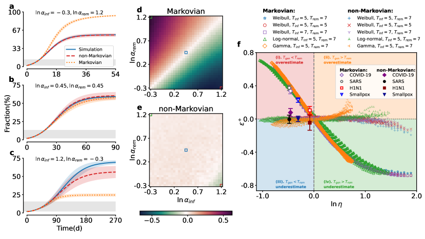
Figure 4: Epidemic Forecasting. a–c: Predicted evolution of the cumulative infected fraction (i.e., sum of infected and removed fractions) by the Markovian (orange dotted curves) and non-Markovian (red dashed curves) theories, in comparison with the Monte Carlo simulations with Weibull time distributions (blue solid curves), for three sets of simulation parameters, respectively. The results are the averages of 100 independent realizations with the standard deviations indicated by the shaded regions. The gray area marks the average cumulative infected fraction for training data selection. d-e: The forecasting errors $\varepsilon^{+}$ of Markovian and non-Markovian theories with respect to the memory-dependent Monte Carlo simulations in the parameter plane of $\ln{\alpha_{\mathrm{inf}}}$ and $\ln{\alpha_{\mathrm{rem}}}$ in the range $[-0.3,1.2]$. The green, blue and red squares mark the parameters of Monte Carlo simulations in a–c, respectively. f: The forecasting errors $\varepsilon^{+}$ from the Markovian and non-Markovian theories for different values of $\ln{\eta}$ under five scenarios of time distribution setting for Monte Carlo simulations. The corresponding estimations for a number of real-world diseases (COVID-19, SARS, H1N1 and Smallpox) are also included.

Using the five scenarios specified in Fig. 2j for memory-dependent Monte Carlo simulations, we obtain the relationship between $\varepsilon^{+}$ and $\ln{\eta}$, as shown in Fig. 4f. It can be seen that, in the Markovian framework, an overestimation arises for $T_{\mathrm{gen}}<T_{\mathrm{rem}}$, and an underestimation occurs for $T_{\mathrm{gen}}>T_{\mathrm{rem}}$. Only when $T_{\mathrm{gen}}=T_{\mathrm{rem}}$ is an accurate estimate achieved. In general, the non-Markovian theory provides much more accurate forecasting than the Markovian theory, especially when $T_{\mathrm{gen}}$ and $T_{\mathrm{rem}}$ are not equal. The results further illustrate that the forms of time distributions or the specific values of $T_{\mathrm{gen}}$, $T_{\mathrm{inf}}$, or $T_{\mathrm{rem}}$ have little impact on forecasting accuracy.

To establish the relevance of these results to real-world diseases, we obtain the $\psi_{\mathrm{inf}}(\tau)$ and $\psi_{\mathrm{rem}}(\tau)$ relations for four known infectious diseases, including COVID-19, SARS, H1N1 influenza, and smallpox, using the information in Refs. [3, 40, 41, 42, 43, 44, 45, 46, 47]. We then calculate the corresponding values of $\varepsilon^{+}$ and $\ln\eta$ based on the Markovian and non-Markovian approaches. As demonstrated in Fig. 4f, the positions of the four diseases in the ($\ln{\eta}$, $\varepsilon^{+}$) plane are consistent with the results of our estimations. Because the data were from the reports of laboratory-confirmed cases incorporating the effects of the quarantine and distancing from susceptible individuals after the confirmation of the diagnosis, $T_{\mathrm{gen}}$ of the four diseases are all smaller than the corresponding values of $T_{\mathrm{rem}}$, leading to some overestimation for the Markovian forecasting results.

Evaluation of vaccination strategies

In the development and application of a theory for disease spreading, assessing the effects of different vaccination strategies is an important task. Here we consider five prioritization strategies for vaccine distribution [6]: individuals under 20 years (denoted as $m=1$), adults between 20 and 49 years ($m=2$), adults above 20 years ($m=3$), adults above 60 years ($m=4$), and all age groups ($m=5$), and implement these strategies in Monte Carlo simulations. Fig. 5a shows the results of epidemic evolution in comparison with those without any vaccination intervention ($m=0$), where the shape parameters are chosen according to $\ln{\alpha_{\mathrm{inf}}}=0.45$ and $\ln{\alpha_{\mathrm{rem}}}=0.45$ ($T_{\mathrm{gen}}=T_{\mathrm{rem}}$). Figs. 5b–c show the results from the Markovian and non-Markovian theories, respectively, with the corresponding fitted parameters for the vaccination strategies in comparison with those without vaccination (see Method for the detailed procedure of vaccination in the theoretical calculation). These results indicate that the Markovian and non-Markovian theories yield the correct epidemic evolution and future outbreaks under different vaccination scenarios.

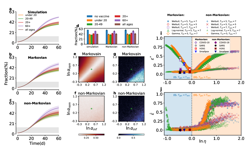
Figure 5: Evaluation of vaccination strategies. a–c: For simulation parameters chosen according to $\ln{\alpha_{\mathrm{inf}}}=0.45$ and $\ln{\alpha_{\mathrm{rem}}}=0.45$, the cumulative infected fraction (i.e., sum of infected and removed fractions) curves from Monte Carlo simulations and the corresponding Markovian and non-Markovian theories with fitting parameters for five vaccination strategies and the case of no vaccination. The average results are obtained from 100 independent realizations with the shaded regions representing the standard deviations. The gray area marks the average cumulative infected fraction for training data selection. d: Vector $\delta$ calculated from the results in Figs. 5a–c. e–f: The prevention evaluation errors $\varepsilon^{*}$ of Markovian and non-Markovian theories for evaluating the effects of vaccination prevention in the parameter plane $(\ln{\alpha_{\mathrm{inf}}},\ln{\alpha_{\mathrm{rem}}})$. The green squares mark the selected parameters in a–c. g–h: The optimization failure probabilities $\hat{\varepsilon}$ arising from the Markovian and non-Markovian within the parameter plane $(\ln{\alpha_{\mathrm{inf}}},\ln{\alpha_{\mathrm{rem}}})$. The green squares mark the selected parameters in a–c. i: The prevention evaluation errors $\varepsilon^{*}$ from the Markovian and non-Markovian theories versus $\ln{\eta}$ under five scenarios of time distribution setting for Monte Carlo simulations. The estimated errors for four real diseases (COVID-19, SARS, H1N1 and Smallpox) are also shown. j: The optimization failure probabilities $\hat{\varepsilon}$ from the Markovian and non-Markovian theories against $\ln{\eta}$ in five different time distribution scenarios for Monte Carlo simulations. The optimization failure probabilities for four real diseases (COVID-19, SARS, H1N1 and Smallpox) are also presented.

To characterize the effectiveness of different vaccination strategies in blocking disease transmission, we introduce a vector, $\delta$, whose $m$-th element quantifies the cumulative infected fraction with the $m$-th vaccination strategy in the steady state: $\delta_{m}=\tilde{c}_{m}$, for $m=0,\ldots,5$. Fig. 5d shows that the $\delta$ vectors from the Monte Carlo simulation, Markovian and non-Markovian theories from Figs. 5a–c, respectively.

We further introduce a metric, the so-called prevention evaluation error $\varepsilon^{*}$, that gauges the ability of the Markovian and non-Markovian theories to estimate the total effectiveness of vaccination, i.e., measuring the disparity between the results calculated by the Markovian or non-Markovian theories and those obtained through Monte Carlo simulations considering various vaccination strategies (see Method for the detailed definition of $\varepsilon^{*}$). Figs. 5e–-f show the average values of $\varepsilon^{*}$ of the two theories in the simulation parameter plane using 100 independent realizations, which are similar to those in Figs. 4d–e, indicating that the error mainly comes from the $R_{0}$ estimation. In general, the Markovian theory performs well only in the diagonal area of the parameter plane where $\alpha_{\mathrm{inf}}=\alpha_{\mathrm{rem}}$, as shown in Fig. 5e, and the non-Markovian theory outperforms the Markovian counterpart in most cases, as shown in Fig. 5f.

Meanwhile, we assess the ability of both the Markovian and non-Markovian theories to detect the optimal vaccination strategy. We also define a quantity, optimization failure probability $\hat{\varepsilon}$, to quantify the probability of a theory failing to identify the optimal strategy, i.e., that leads to the lowest cumulative infection among the five strategies (see Method for the detailed definition of $\hat{\varepsilon}$). Figs. 5g–-h illustrate the results of $\hat{\varepsilon}$ for the two theories within the parameter plane $(\ln{\alpha_{\mathrm{inf}}},\ln{\alpha_{\mathrm{rem}}})$. While the non-Markovian theory still demonstrates superior performance, the Markovian approach proves capable of identifying the optimal strategy across a significantly larger parameter space compared to the Markovian results depicted in Figure 5e.

We obtain the relationships between $\varepsilon^{*}$ and $\ln{\eta}$, as well as between $\hat{\varepsilon}$ and $\ln{\eta}$, as shown in Fig. 5i–j with the same five time-distribution scenarios as in Fig. 2j. In all cases of Fig. 5i, $\varepsilon^{*}$ reaches a minimum for $\ln{\eta}=0$ and increases as $\ln{\eta}$ deviates from zero. The agreement of the results from the five scenarios further illustrates that the forms of time distributions or the specific values of $T_{\mathrm{gen}}$, $T_{\mathrm{inf}}$, or $T_{\mathrm{rem}}$ play little role in the errors in vaccination evaluation. Fig. 5i also includes the values of $\varepsilon^{*}$ for the real-world infectious diseases COVID-19, SARS, H1N1 influenza, and smallpox, which are consistent with those from the non-Markovian and Markovian theories. Regarding the results depicted in Fig. 5j, it is observed that the non-Markovian theories consistently outperform the Markovian counterparts. On the other hand, within a wide range of $\ln\eta$ values around 0, the Markovian theories successfully identify the optimal vaccination strategy among various commonly employed ones. When the value of $\ln\eta$ significantly deviates from 0, Markovian theories become ineffective in determining the optimal strategy. (Note that on the left side of Fig. 5j, we only present the failures of Markovian theories to identify the optimal strategy in the Monte Carlo simulations with log-normal distribution. This is primarily due to the fact that the parameters associated with the Weibull and gamma distributions fall outside the acceptable range when we keep $T_{\mathrm{inf}}$ and $T_{\mathrm{rem}}$ fixed to modify $\ln\eta$ to a very low value.) Furthermore, we demonstrate that even when employing Markovian approaches, the optimal vaccination strategy can still be determined among the five strategies considered for the four distinct real diseases.

Conducting accurate evaluations in prevention serves as the sufficient condition of the successful identification of the optimal strategy. In comparison to the prevention evaluation errors $\varepsilon^{*}$ of Markovian theories, the optimization failure probability $\hat{\varepsilon}$ exhibits a wider range of $\ln\eta$ values that result in the lowest value. The lack of mathematical continuity among the five strategies is the primary reason for this. It indicates that there is no smooth transition or mathematical relationship connecting these strategies, resulting in the rank of the strategies not changing promptly when the value of $\ln\eta$ deviates from 0. Therefore, only significant errors from the Markovian theories can result in the failure to detect the optimal strategy. Based on this analysis, the extent to which $\ln\eta$ deviates from 0, leading to the failure of Markovian theories, as well as whether such failure will occur, depends on the selection of the tested strategies.

Discussion

The COVID-19 pandemic has emphasized the importance of investigating disease transmission in human society through modeling. Empirical observations have consistently demonstrated strong memory effects in real-world transmission phenomena. The initial transient stage of an epidemic is critical for data collection, prediction, and articulation of control strategies, but an accurate non-Markovian model presents difficulties. In contrast, a Markovian model offers great advantages in parameter estimation, computation, and analyses. Uncovering the conditions under which Markovian modeling is suitable for transient epidemic dynamics is necessary.

We have developed a comprehensive mathematical framework for both Markovian and non-Markovian compartmentalized SIR disease transmissions in an age-stratified population, which allows us to identify two types of equivalence between Markovian and non-Markovian dynamics: in the steady state and transient phase of the epidemic. Our theoretical analysis reveals that, in the steady state, non-Markovian (memory-dependent) transmissions are always equivalent to the Markovian (memoryless) dynamics. However, transient-state equivalence is approximate and holds when the average generation and removal times match each other. In particular, when the average generation time is approximately equal to the average removal time, the disease transmission and removal of an infected individual exhibit a memoryless correlation, thereby minimizing the memory effects of the dynamical process. This results in highly accurate results from the Markovian theory that captures the characteristics of memory-dependent transmission based solely on the early epidemic curves. Our analysis also suggests that the Markovian accuracy is mainly determined by the value of generation-to-removal time ratio in disease transmission, where a larger-than-one (smaller-than-one) ratio can lead to underestimation (overestimation) of the basic reproduction number and epidemic forecasting, as well as the errors in the evaluation of control or prevention measures. The estimation accuracy primarily depends on this ratio, but is not significantly affected by the specific values and distribution forms of the various times associated with the epidemic. This property exhibits substantial practical importance, because the average generation and removal times can be readily assessed based on sparse data collected from the transient phase of the epidemic, but to estimate their distributions with only sparse data is infeasible. These results provide deeper quantitative insights into the influence of memory effects on epidemic transmissions, leading to a better understanding of the connection and interplay between Markovian and non-Markovian dynamics.

There were previous studies of the equivalence between Markovian and non-Markovian transmission in the SIS model [24, 25, 21]. However, these studies addressed the steady-state equivalence rather than the transient-state equivalence. To our knowledge, our work is the first to investigate the transient-state equivalence of the SIR model. In addition, previous studies mainly examined the impact of the average generation time on the transmission dynamics, such as how the shape of the generation time distribution affects the estimation of $R_{0}$ [58] or the use of serial time distributions in estimating $R_{0}$ during an epidemic [50]. There was a gap in the literature regarding how generation times affect the accuracy of different models. Our paper fills this gap by providing a criterion for using Markovian frameworks to model memory-dependent transmission based on the relationship between the average generation and removal times.

From an application perspective, our study suggests that the impact of the time distribution forms on Markovian estimation accuracy is minimal, making it easier to select models between Markovian and non-Markovian dynamics in the initial outbreak of an epidemic based only on the generation-to-removal time ratio. This insight is especially useful since detailed time distribution forms are often harder to detect than their corresponding mean values. In addition, we note that in previous studies, it was observed that in various scenarios, serial intervals, albeit with larger variances, are anticipated to possess a consistent mean value with the average generation time and are more straightforward to measure [3, 50, 51, 52, 53, 54]. Given the practical difficulties in observing the generation time, our finding of minimal impact from the distribution forms suggests that the average serial interval can be utilized as a substitute of the average generation time to determine the applicability of the Markovian theories for modeling purposes without compromising accuracy, although numerous studies have indicated that replacing the generation time distribution with the serial interval distribution may affect the analysis of transmission dynamics [50, 60, 49]. Meanwhile, based on the Eq. (15), if we determine the ratio of generation-to-removal time, the estimated $R_{0}$ obtained through the Markovian approach can be adjusted to approximate the true. And our web-based application showcases the demonstration of rectifying $R_{0}$ and epidemic forecasting [55].

Our study highlights the critical importance of accurately quantifying $R_{0}$ for achieving precise epidemic forecasting and prevention evaluation. A previous work [59] revealed that the value of $R_{0}$ depends on three key components: the duration of the infectious period (e.g., $\psi_{\mathrm{rem}}(\tau)$), the probability of infection resulting from a single contact between an infected individual and a susceptible one (e.g., $\psi_{\mathrm{inf}}(\tau)$), and the number of new susceptible individuals contacted per unit of time. However, given the practical limitations inherent in obtaining all three components, numerous methods have been developed for estimating $R_{0}$. Although our work presents a specific approach, which fits the parameters of exponential or non-exponential time distribution by using the initial outbreak curves, it is not the only one available. For example, when contact patterns are unknown, $R_{0}$ can be estimated by fitting the growth rate $g$ and the generation time distribution $\psi_{\mathrm{gen}}(\tau)$, and then applying them in the Euler-Lotka equation [59, 58, 50]. However, since the focus of our work is on epidemic forecasting and evaluation of prevention measure, $R_{0}$ can be directly calculated once $\psi_{\mathrm{inf}}(\tau)$ and $\psi_{\mathrm{rem}}(\tau)$ are fitted, without requiring the fitting of any additional quantity. The estimation of $R_{0}$ can also be achieved by using data in the steady state, such as the final size of an epidemic or equilibrium conditions [59]. However, this method is not suitable for the transient phase where only early-stage curves are available. Utilizing the approach delineated in this paper is practically more appropriate for estimating $R_{0}$.

While our study focused on transmission within the SIR framework, extension to SEIR or SIS models is feasible. While we emphasized the significance of the transient-state equivalence in disease transmission, transient dynamics are more relevant or even more crucial than the steady state in nonlinear dynamical systems [61]. For example, in ecological systems, transient dynamics play a vital role in empirical observations and are therefore a key force driving natural evolution [62, 63, 64, 65, 66, 67]. In neural dynamics, transient changes in neural activity can mediate synaptic plasticity, a crucial mechanism for learning and memory [68, 69, 70]. Therefore, the identification of suitable conditions for choosing between Markovian and non-Markovian dynamics may not be limited to transmission dynamics alone and may serve as a valuable reference for other fields as well.

Taken together, our study establishes an approximate equivalence between Markovian and non-Markovian dynamics in the transient state, assuming that time distributions follow Weibull forms (see Supplementary Note 3 for details). While the applicability of our findings to most synthetic and empirical distributions has been analyzed qualitatively, a quantitative analysis requires further studies. For extreme cases with non-Weibull distributions, the transmission should be evaluated using other specific methods. While we have provided a qualitative analysis of the mechanism underlying why time distribution forms have minimal impacts on the errors of Markovian estimations, a more rigorous theoretical analysis is needed and requires further exploration. In addition, due to the complexity of the nonlinear transmission, our study has produced a semi-empirical relationship to estimate the overestimation and underestimation of Markovian methods. Further research is required to develop a rigorous formula that can accurately predict these effects.

Methods

Monte Carlo simulation

In the simulation, we classify $N$ individuals into $n$ subgroups based on the age distribution p. The index of the subgroup to which an individual belongs is denoted by $l$ (where $0\leq l\leq n-1$), and the index of the individual within the subgroup is denoted by $u$ (where $0\leq u\leq\mathbf{\mathit{p}}_{l}N$). The state of the $u$-th individual in the $l$-th subgroup is represented by $X_{lu}$, which includes the states $S$ (susceptible), $I$ (infected), $W$ (recovered), and $D$ (dead), where $W$ and $D$ both represent $R$ (removed). For each individual, we also record the absolute time of infection and removal using two variables: $T_{lu}^{\mathrm{inf}}$ and $T_{lu}^{\mathrm{rem}}$, respectively. The absolute time of the system is denoted by $T$, and we implement the total spreading simulation step by step using a finite time step $\Delta T$ as follows:

• Initialization: set $T=0$, $X_{lu}$ for every individual is set to $S$.

• Set infection seeds: choose a set of individuals as the infection seeds and the corresponding $X_{lu}$ are set to $I$, the corresponding $T_{lu}^{\mathrm{inf}}$ are set to 0, and $T_{lu}^{\mathrm{rem}}$ are set to a random value following the removal time distribution $\psi_{\mathrm{rem}}(\tau)$.

• Infection of one step: calculate the infection rate, $\hat{\omega}_{lu}^{\mathrm{inf}}(T)$, of infected individual $u$ in age group $l$ during the current time step by

  $$\hat{\omega}_{lu}^{\mathrm{inf}}(T)=1-\Psi_{\mathrm{inf}}(T-T_{lu}^{\mathrm{inf}}+\Delta T)/\Psi_{\mathrm{inf}}(T-T_{lu}^{\mathrm{inf}}).$$

  The probability $\bar{\omega}_{l}^{\mathrm{inf}}(T)$ of each susceptible individual in age group $l$ being infected can be calculated by

  $$\bar{\omega}_{l}^{\mathrm{inf}}(T)=\sum_{m=1}^{n}{\mathbf{\mathit{p}}_{m}[1-(1-\frac{\sum_{v\in\mathcal{I}_{m}}{\hat{\omega}_{mv}^{\mathrm{inf}}(T)}}{\mathbf{\mathit{p}}_{m}N})^{k\mathbf{\mathit{A}}_{lm}}]},$$

  where $\mathcal{I}_{m}$ is the index set of the infected individual in age group $m$. The number of the susceptible individuals being infected in a age group follows a binomial distribution $B(s_{l}(T)\mathbf{\mathit{p}}_{l}N,\bar{\omega}_{l}^{\mathrm{inf}}(T))$, where $s_{l}(T)$ denotes the fraction of susceptible individuals in age group $l$ at time $T$. Then generate a random number $N_{l}(T)$ following this binomial distribution and set the $N_{l}(T)$ individuals as $I$ state. The corresponding $T_{lu}^{\mathrm{inf}}$ of the new infected individuals are set to the current $T$ and $T_{lu}^{\mathrm{rem}}$ are set to $T_{\mathrm{rem}}+T$, where the random $T_{\mathrm{rem}}$ follow the removal time distribution $\psi_{\mathrm{rem}}(\tau)$.

• Check if $T_{lu}^{\mathrm{rem}}$ of each infected individual is during the current time step. If this condition is satisfied, set their state to $D$ with a probability of death and to $W$ otherwise. Then let $T=T+\Delta T$.

• Repeat the process iii) and iv), until no individual with $I$ index exists.

Time distributions

In the Monte Carlo simulations, we employ three types of time distributions, i.e., Weibull, log-normal, and gamma, to describe the memory-dependent transmission process.

For Weibull time distribution, it follows:

$$\psi(\tau)=\frac{\alpha}{\beta}(\frac{\tau}{\beta})^{\alpha-1}e^{-(\frac{\tau}{\beta})^{\alpha}},$$

where $\alpha$ and $\beta$ denote the shape and scale parameters, respectively.

The log-normal time distribution is defined as follows:

$$\psi(\tau)=\frac{1}{\tau\beta\sqrt{2\pi}}\exp(-\frac{(\ln\tau-\alpha)^{2}}{2\beta^{2}}).$$

The gamma time distribution is expressed as follows:

$$\psi(\tau)=\frac{1}{\Gamma(\alpha)\beta^{\alpha}}\tau^{\alpha-1}e^{-\frac{\tau}{\beta}},$$

where $\Gamma(\cdot)$ denotes gamma function, while $\alpha$ and $\beta$ represent the shape and scale parameters, respectively.

For each type of time distribution, denoted as $\psi(\tau)$, it can be either $\psi_{\mathrm{inf}}(\tau)$ or $\psi_{\mathrm{rem}}(\tau)$. Similarly, the parameter $\alpha$ can take either $\alpha_{\mathrm{inf}}$ or $\alpha_{\mathrm{rem}}$, and the parameter $\beta$ can be either $\beta_{\mathrm{inf}}$ or $\beta_{\mathrm{rem}}$.

Additionally, the survival function could calculated by:

$$\Psi(\tau)=\int_{\tau}^{+\infty}{\psi(\tau^{\prime})d\tau^{\prime}},$$

while the hazard function could deducted by:

$$\omega(\tau)=\frac{\psi(\tau)}{\int_{\tau}^{+\infty}{\psi(\tau^{\prime})d\tau^{\prime}}}.$$

The survival function $\Psi(\tau)$ can be either $\Psi_{\mathrm{inf}}(\tau)$ or $\Psi_{\mathrm{rem}}(\tau)$, and the hazard function $\omega(\tau)$ can take either $\omega_{\mathrm{inf}}(\tau)$ or $\omega_{\mathrm{rem}}(\tau)$.

Derivation of semi-empirical estimation of basic reproduction number

Intuitively, the period of $T_{\mathrm{rem}}$ can accommodate $T_{\mathrm{rem}}/T_{\mathrm{gen}}=1/\eta$ time intervals of length $T_{\mathrm{gen}}$, corresponding to the result of $1/\eta$ generations of infections. This can lead to an exponential increase in the number of infections during $T_{\mathrm{rem}}$. This intuition suggests a relationship between the fitted basic reproduction number $\hat{R}_{0}$ and the actual $R_{0}$, which can be expressed as an exponential function:

$$\hat{R}_{0}=R_{0}^{f(1/\eta)},$$

where $f(\cdot)$ is a monotonically increasing function that satisfies three conditions. First, $f(1)=1$, indicating that $\hat{R}_{0}$ can be accurately estimated when $T_{\mathrm{gen}}=T_{\mathrm{rem}}$. Second, $f(0)=0$, meaning that if $T_{\mathrm{rem}}$ is an extremely small fraction of $T_{\mathrm{gen}}$, the transmission will take a long time to reach the steady state, causing the curve to be flat in the initial stage and potentially causing the Markovian fitting to produce the estimate $\hat{R}_{0}=1$. Third, $f(+\infty)=+\infty$, implying that if $T_{\mathrm{rem}}$ is extremely large compared to $T_{\mathrm{gen}}$, the transmission will quickly reach the final prevalence, causing the Markovian fitting to give an extremely large estimate of $\hat{R}_{0}$. Because the actual transmission process involves many complicated nonlinear relationships, identifying the specific form of the function $f(\cdot)$ is a challenging task. We thus assume

$$f(x)=x^{a},$$

where $a$ is an unknown positive coefficient. This leads to Eq. (15).

Definition of errors

The difference $\varepsilon$ between non-Markovian and the corresponding Markovian results calculated from Eqs. (13–14) is defined as:

$$\varepsilon=\sum_{x,x^{*}\in\{(s,s^{*}),(i,i^{*}),(r,r^{*})\}}{\frac{\|x^{*}-x\|_{2,T}}{\|x\|_{2,T}}}$$

where the pairs $(s,s^{*})$, $(i,i^{*})$ and $(r,r^{*})$ correspond to the non-Markovian and Markovian susceptible, infected and removed curves, respectively. The 2-norm $\|\cdot\|_{2,T}$ on time duration $T$ ensures that $\varepsilon$ measures the “distance” between non-Markovian and the Markovian transient states. It is not appropriate to set $T$ as the total transmission period because the cumulative infected fraction approaches the final value asymptotically, making it difficult to determine the exact time point of the steady state. To address this issue, we choose $T$ as $[0,\tilde{t}_{\theta}]$, where $\tilde{t}_{\theta}$ is the time when the cumulative infected fraction $c(t)$ reaches the $\theta$ percentile point within the range that spans from its initial value ($\acute{c}$) to its final value ($\tilde{c}$). The value of $\theta$ in Fig. 2j is selected as 50 (see Supplementary Note 6 for more selection of $\theta$ and detailed analysis).

The forecasting error $\varepsilon^{+}$ that evaluates whether a theory overestimates or underestimates the steady-state cumulative infected fraction is defined as:

$$\varepsilon^{+}=\frac{c(\tilde{t})-\hat{c}(\tilde{t})}{\hat{c}(\tilde{t})},$$

where $\tilde{t}$ denotes the time when the stochastic simulation reaches the steady state when no infection occurs in the population, $c(\tilde{t})$ and $\hat{c}(\tilde{t})$ are the cumulative infected fractions from theory and simulation, respectively. A positive value of $\varepsilon^{+}$ indicates overestimation, whereas a negative value indicates underestimation.

The prevention evaluation error $\varepsilon^{*}$, that gauges the ability of the Markovian and non-Markovian theories to estimate the total effectiveness of vaccination, is defined as:

$$\varepsilon^{*}=\frac{\|\hat{\delta}-\delta\|_{2}}{\|\hat{\delta}\|_{2}},$$

where $\hat{\delta}$ is the result from Monte Carlo simulation and $\|\cdot\|_{2}$ is the 2-norm of a vector.

The optimization failure probability $\hat{\varepsilon}$, which measures the probability that a theory fails to identify the optimal vaccination strategy, is defined as:

$$\hat{\varepsilon}=\frac{\sum_{l=1}^{z}{\xi^{(l)}}}{z},$$

where

$$\xi^{(l)}=\begin{cases}0&\text{if }\operatorname*{argmin}\hat{\sigma}^{(l)}=\operatorname*{argmin}\sigma^{(l)}\\ 1&\text{otherwise}\end{cases},$$

$\hat{\sigma}^{(l)}$ and $\sigma^{(l)}$ represent the vectors, $\hat{\sigma}$ and $\sigma$, for the $l$-th experiment, respectively, and $z$ denotes the total number of experiments (in this paper, $z$ is set to 100). Consequently, $\hat{\varepsilon}$ quantifies the fraction of experiments in which a theory fails to identify the optimal vaccination strategy, and serves as a measure of the probability of failure in optimizing the vaccination strategy.

Fitting method

Because the removal process is independent of the infection one, we divide the fitting method into two parts: removal parameter fitting and infection parameter fitting. Specifically, we use $c_{\mathrm{init}}^{*}$ and $r_{\mathrm{init}}^{*}$ to denote the cumulative infected and removed fractions in the initial stage of a Monte Carlo simulation. These two types of data are substituted into the Eq. (3) to fit the parameters of $\psi_{\mathrm{rem}}(\tau)$. Likewise, we use $c_{l,\mathrm{init}}^{*}$ to denotes the cumulative infected fraction of age group $l$ in the initial stage of a Monte Carlo simulation and $s_{l,\mathrm{init}}^{*}=1-c_{l,\mathrm{init}}^{*}$ represents the corresponding susceptible fraction. After obtaining the removal parameters, these two types of data are put into Eq. (1) to fit the infection time distribution parameters.

In our study, we selected the curves of all states that occurred prior to the time point at which the cumulative infected fraction reached a specific percentile (e.g., $20\%$) situated between the initial and steady cumulative infected fractions, as the training data. Choosing a specific time period as the training data may not be appropriate, as it can result in an overabundance of data points for fitting due to some instances of fast transmission already having reached the steady state, while some instances of slow transmission may not have spread out yet, leading to too few data points.

Vaccination method

We assume that the individuals will build enough immune protection from the disease $\kappa$ days after vaccination with the probability $\rho$. In Monte Carlo simulations, the susceptible individual who gets vaccinated and the corresponding time $T_{\mathrm{vac}}$ are associated with the probability $\rho$, and the absolute time becomes $T_{\mathrm{vac}}+\kappa$. If this individual has not been infected, he/she will be set to a state called protected state, indicating that this individual is protected from the disease.

When a fraction of individuals in age group $l$ get vaccinated, the detailed vaccination fraction $\upsilon_{l}$, susceptible time $t_{\mathrm{vac}}$ and the fraction of susceptible individuals $s_{l}(t_{\mathrm{vac}})$ are recorded. When the absolute time reaches $T_{\mathrm{vac}}+\kappa$, the corresponding value of $s_{l}(t_{\mathrm{vac}}+\kappa)$ will be set as $s_{l}(t_{\mathrm{vac}}+\kappa)\rho\frac{\upsilon_{l}}{s_{l}(t_{\mathrm{vac}})}$.

Data Availability

All relevant data are available at https://github.com/fengmi9312/Validity-of-Markovian-for-Memory/tree/main/FigureData.

Code Availability

The web-based application can be visited at https://cns.hkbu.edu.hk/toolbox/Validity-of-Markovian-for-Memory/main.html. The GitHub repository, which includes the source code for all the figure results, the web-based application, and an additional Python application, can be accessed at https://github.com/fengmi9312/Validity-of-Markovian-for-Memory.git.

Author Contributions

M.F., L.T. and C.-S.Z. designed research; M.F. performed research; L.T. and C.-S.Z. contributed analytic tools; M.F., L.T. and C.-S.Z. analysed data; M.F., L.T., Y.-C.L. and C.-S.Z. discussed the results and wrote the paper.

Competing Interests

The authors declare no competing interests.

Correspondence

To whom correspondence should be addressed: liangtian@hkbu.edu.hk, cszhou@hkbu.edu.hk

References

- [1] Dong, E., Du, H. & Gardner, L. An interactive web-based dashboard to track covid-19 in real time. Lancet Infect. Dis. 20, 533–534 (2020).
- [2] Mishra, S. K. & Tripathi, T. One year update on the covid-19 pandemic: Where are we now? Acta Trop. 214, 105778 (2021).
- [3] Ferretti, L. et al. Quantifying sars-cov-2 transmission suggests epidemic control with digital contact tracing. Science 368, eabb6936 (2020).
- [4] Giordano, G. et al. Modeling vaccination rollouts, sars-cov-2 variants and the requirement for non-pharmaceutical interventions in italy. Nat. Med. 27, 993–998 (2021).
- [5] Jentsch, P. C., Anand, M. & Bauch, C. T. Prioritising covid-19 vaccination in changing social and epidemiological landscapes: a mathematical modelling study. Lancet Infect. Dis. 21, 1097–1106 (2021).
- [6] Bubar, K. M. et al. Model-informed covid-19 vaccine prioritization strategies by age and serostatus. Science 371, 916–921 (2021).
- [7] Buckner, J. H., Chowell, G. & Springborn, M. R. Dynamic prioritization of covid-19 vaccines when social distancing is limited for essential workers. Proc. Natl Acad. Sci. 118, e2025786118 (2021).
- [8] Goldstein, J. R., Cassidy, T. & Wachter, K. W. Vaccinating the oldest against covid-19 saves both the most lives and most years of life. Proc. Natl Acad. Sci. 118, e2026322118 (2021).
- [9] Viana, J. et al. Controlling the pandemic during the sars-cov-2 vaccination rollout. Nat. Commun. 12, 1–15 (2021).
- [10] Matrajt, L., Eaton, J., Leung, T. & Brown, E. R. Vaccine optimization for covid-19: Who to vaccinate first? Sci. Adv. 7, eabf1374 (2021).
- [11] Matrajt, L. et al. Optimizing vaccine allocation for covid-19 vaccines shows the potential role of single-dose vaccination. Nat. Commun. 12, 1–18 (2021).
- [12] Zhao, S. et al. Preliminary estimation of the basic reproduction number of novel coronavirus (2019-ncov) in china, from 2019 to 2020: A data-driven analysis in the early phase of the outbreak. Int. J. Infect. Dis. 92, 214–217 (2020).
- [13] Billah, M. A., Miah, M. M. & Khan, M. N. Reproductive number of coronavirus: A systematic review and meta-analysis based on global level evidence. PloS one 15, e0242128 (2020).
- [14] Liu, Y. & Rocklöv, J. The effective reproductive number of the omicron variant of sars-cov-2 is several times relative to delta. Journal of Travel Medicine 29, taac037 (2022).
- [15] Metcalf, C. J. E. & Lessler, J. Opportunities and challenges in modeling emerging infectious diseases. Science 357, 149–152 (2017).
- [16] Riley, S. Large-scale spatial-transmission models of infectious disease. Science 316, 1298–1301 (2007).
- [17] Levin, S. A., Grenfell, B., Hastings, A. & Perelson, A. S. Mathematical and computational challenges in population biology and ecosystems science. Science 275, 334–343 (1997).
- [18] Pastor-Satorras, R., Castellano, C., Van Mieghem, P. & Vespignani, A. Epidemic processes in complex networks. Rev. Mod. Phys. 87, 925 (2015).
- [19] Lambiotte, R., Tabourier, L. & Delvenne, J.-C. Burstiness and spreading on temporal networks. Eur. Phys. J. B 86, 1–4 (2013).
- [20] Lin, Z.-H. et al. Non-markovian recovery makes complex networks more resilient against large-scale failures. Nat. Commun. 11, 1–10 (2020).
- [21] Cator, E., Van de Bovenkamp, R. & Van Mieghem, P. Susceptible-infected-susceptible epidemics on networks with general infection and cure times. Phys. Rev. E 87, 062816 (2013).
- [22] Boguná, M., Lafuerza, L. F., Toral, R. & Serrano, M. Á. Simulating non-markovian stochastic processes. Phys. Rev. E 90, 042108 (2014).
- [23] Van Mieghem, P. & Van de Bovenkamp, R. Non-markovian infection spread dramatically alters the susceptible-infected-susceptible epidemic threshold in networks. Phys. Rev. Lett. 110, 108701 (2013).
- [24] Starnini, M., Gleeson, J. P. & Boguñá, M. Equivalence between non-markovian and markovian dynamics in epidemic spreading processes. Phys. Rev. Lett. 118, 128301 (2017).
- [25] Feng, M., Cai, S.-M., Tang, M. & Lai, Y.-C. Equivalence and its invalidation between non-markovian and markovian spreading dynamics on complex networks. Nat. Commun. 10, 1–10 (2019).
- [26] Min, B., Goh, K.-I. & Kim, I.-M. Suppression of epidemic outbreaks with heavy-tailed contact dynamics. EPL 103, 50002 (2013).
- [27] Karrer, B. & Newman, M. E. Message passing approach for general epidemic models. Phys. Rev. E 82, 016101 (2010).
- [28] Wang, Y., Chakrabarti, D., Wang, C. & Faloutsos, C. Epidemic spreading in real networks: An eigenvalue viewpoint. In 22nd International Symposium on Reliable Distributed Systems, 2003. Proceedings., 25–34 (IEEE, 2003).
- [29] Chakrabarti, D., Wang, Y., Wang, C., Leskovec, J. & Faloutsos, C. Epidemic thresholds in real networks. ACM Trans. Inf. Syst. Secur. 10, 1–26 (2008).
- [30] Keeling, M. J. & Grenfell, B. T. Disease extinction and community size: modeling the persistence of measles. Science 275, 65–67 (1997).
- [31] Barabasi, A.-L. The origin of bursts and heavy tails in human dynamics. Nature 435, 207–211 (2005).
- [32] Gonzalez, M. C., Hidalgo, C. A. & Barabasi, A.-L. Understanding individual human mobility patterns. Nature 453, 779–782 (2008).
- [33] Simini, F., González, M. C., Maritan, A. & Barabási, A.-L. A universal model for mobility and migration patterns. Nature 484, 96–100 (2012).
- [34] Pappalardo, L. et al. Returners and explorers dichotomy in human mobility. Nat. Commun. 6, 1–8 (2015).
- [35] Yan, X.-Y., Wang, W.-X., Gao, Z.-Y. & Lai, Y.-C. Universal model of individual and population mobility on diverse spatial scales. Nat. Commun. 8, 1–9 (2017).
- [36] Bratsun, D., Volfson, D., Tsimring, L. S. & Hasty, J. Delay-induced stochastic oscillations in gene regulation. Proc. Natl Acad. Sci. 102, 14593–14598 (2005).
- [37] Scalas, E., Kaizoji, T., Kirchler, M., Huber, J. & Tedeschi, A. Waiting times between orders and trades in double-auction markets. Physica A 366, 463–471 (2006).
- [38] Vazquez, A., Racz, B., Lukacs, A. & Barabasi, A.-L. Impact of non-poissonian activity patterns on spreading processes. Phys. Rev. Lett. 98, 158702 (2007).
- [39] Min, B., Goh, K.-I. & Vazquez, A. Spreading dynamics following bursty human activity patterns. Phys. Rev. E 83, 036102 (2011).
- [40] Moghadas, S. M. et al. The implications of silent transmission for the control of covid-19 outbreaks. Proc. Natl Acad. Sci. 117, 17513–17515 (2020).
- [41] Lauer, S. A. et al. The incubation period of coronavirus disease 2019 (covid-19) from publicly reported confirmed cases: estimation and application. Ann. Intern. Med. 172, 577–582 (2020).
- [42] Gatto, M. et al. Spread and dynamics of the covid-19 epidemic in italy: Effects of emergency containment measures. Proc. Natl Acad. Sci. 117, 10484–10491 (2020).
- [43] Li, R. et al. Substantial undocumented infection facilitates the rapid dissemination of novel coronavirus (sars-cov-2). Science 368, 489–493 (2020).
- [44] Buitrago-Garcia, D. et al. Occurrence and transmission potential of asymptomatic and presymptomatic sars-cov-2 infections: A living systematic review and meta-analysis. PLoS Med. 17, e1003346 (2020).
- [45] Organization, W. H. et al. Consensus document on the epidemiology of severe acute respiratory syndrome (sars). Tech. Rep., World Health Organization (2003).
- [46] Chowell, G. et al. Model parameters and outbreak control for sars. Emerg. Infect. Dis. 10, 1258 (2004).
- [47] Eichner, M. & Dietz, K. Transmission potential of smallpox: estimates based on detailed data from an outbreak. Am. J. Epidemiol. 158, 110–117 (2003).
- [48] Grassly, N. C. & Fraser, C. Mathematical models of infectious disease transmission. Nature Reviews Microbiology 6, 477–487 (2008).
- [49] Ganyani, T. et al. Estimating the generation interval for coronavirus disease (covid-19) based on symptom onset data, march 2020. Eurosurveillance 25, 2000257 (2020).
- [50] Park, S. W. et al. Forward-looking serial intervals correctly link epidemic growth to reproduction numbers. Proc. Natl. Acad. Sci. U.S.A. 118, e2011548118 (2021).
- [51] Svensson, Å. A note on generation times in epidemic models. Math. Biosci. 208, 300–311 (2007).
- [52] Klinkenberg, D. & Nishiura, H. The correlation between infectivity and incubation period of measles, estimated from households with two cases. J. Theor. Biol. 284, 52–60 (2011).
- [53] te Beest, D. E., Wallinga, J., Donker, T. & van Boven, M. Estimating the generation interval of influenza a (h1n1) in a range of social settings. Epidemiology 244–250 (2013).
- [54] Champredon, D., Dushoff, J. & Earn, D. J. Equivalence of the erlang-distributed seir epidemic model and the renewal equation. SIAM J. Appl. Math. 78, 3258–3278 (2018).
- [55] Feng, M., Tian, L., Lai, Y.-C. & Zhou, C. Web-based application for generation time distribution and error rectification of markovian modeling. https://cns.hkbu.edu.hk/toolbox/Validity-of-Markovian-for-Memory/main.html (2023).
- [56] United Nations, Department of Economic and Social Affairs, Population Division. World population prospects 2019 (2021). URL https://population.un.org/wpp/. Accessed on 29 June 2021.
- [57] Prem, K., Cook, A. R. & Jit, M. Projecting social contact matrices in 152 countries using contact surveys and demographic data. PLoS Comput. Biol. 13, e1005697 (2017).
- [58] Wallinga, J. & Lipsitch, M. How generation intervals shape the relationship between growth rates and reproductive numbers. Proc. R. Soc. B 274, 599–604 (2007).
- [59] Dietz, K. The estimation of the basic reproduction number for infectious diseases. Stat. Methods Med. Res. 2, 23–41 (1993).
- [60] Britton, T. & Scalia Tomba, G. Estimation in emerging epidemics: biases and remedies. J. R.Soc. Interface 16, 20180670 (2019).
- [61] Lai, Y.-C. & Tél, T. Transient Chaos - Complex Dynamics on Finite Time Scales (Springer, New York, 2011).
- [62] Hastings, A. & Higgins, K. Persistence of transients in spatially structured ecological models. Science 263, 1133–1136 (1994).
- [63] Hastings, A. Transients: the key to long-term ecological understanding? Trends Ecol. Evol. 19, 39–45 (2004).
- [64] Hastings, A. Timescales and the management of ecological systems. Proc. Natl Acad. Sci. 113, 14568–14573 (2016).
- [65] Hastings, A. et al. Transient phenomena in ecology. Science 361, eaat6412 (2018).
- [66] Morozov, A. et al. Long transients in ecology: Theory and applications. Phys. Life Rev. 32, 1–40 (2020).
- [67] Meng, Y., Lai, Y.-C. & Grebogi, C. Tipping point and noise-induced transients in ecological networks. J. R. Soc. Interface 17, 20200645 (2020).
- [68] Sjöström, P. J., Turrigiano, G. G. & Nelson, S. B. Rate, timing, and cooperativity jointly determine cortical synaptic plasticity. Neuron 32, 1149–1164 (2001).
- [69] Martin, S. J., Grimwood, P. D. & Morris, R. G. Synaptic plasticity and memory: an evaluation of the hypothesis. Annual review of neuroscience 23, 649–711 (2000).
- [70] Kandel, E. R. The molecular biology of memory storage: a dialogue between genes and synapses. Science 294, 1030–1038 (2001).