The dynamics of Measurable pseudo-Anosov maps

Abstract.

We study the dynamics of measurable pseudo-Anosov homeomorphisms of surfaces, a generalization of Thurston’s pseudo-Anosov homeomorphisms. A measurable pseudo-Anosov map has a transverse pair of full measure turbulations consisting of streamlines which are dense immersed lines: these turbulations are equipped with measures which are expanded and contracted uniformly by the homeomorphism. The turbulations need not have a good product structure anywhere, but have some local structure imposed by the existence of tartans: bundles of unstable and stable streamline segments which intersect regularly, and on whose intersections the product of the measures on the turbulations agrees with the ambient measure.

We prove that measurable pseudo-Anosov maps are transitive, have dense periodic points, sensitive dependence on initial conditions, and are ergodic with respect to the ambient measure.

Measurable pseudo-Anosovs maps were introduced in [6], where we constructed a parameterized family of non-conjugate examples on the sphere.

1. Introduction

One of the groundbreaking results proved by William Thurston in the late 1970s and early 1980s was his Classification Theorem for isotopy classes of surface homeomorphisms [19, 13]. A large part of the groundwork for this theorem was carried out between the late 1920s and the early 1940s by Jakob Nielsen, but it was the introduction by Thurston of pseudo-Anosov homeomorphisms which completed the classification. There are isotopy classes containing homeomorphisms which, after finitely many iterates, become the identity: these are of finite order. There are isotopy classes which are reducible in the sense that it is possible to cut the surface up into topologically simpler surfaces and to study the first return map to each of these simpler pieces. If neither of these two possibilities occurs, then there is an essentially unique pseudo-Anosov map in the class. These pseudo-Anosov maps are ‘simplest’ in their isotopy class, which implies, among other things, that all maps in the class have infinitely many periodic orbits, of infinitely many periods, and have positive topological entropy. Thus the fundamentally topological problem of classifying isotopy classes has a solution with strong dynamical content.

The Classification Theorem applies to surfaces of finite topological type, that is, to compact surfaces from which finitely many points have been removed. Dynamicists have often put this theorem to use in studying surface dynamics by finding periodic orbits, removing them from the surface (which might have been the sphere or the disk, say, in which all orientation-preserving homeomorphisms are isotopically trivial), and applying Thurston’s theorem to the isotopy class on the punctured surface thus obtained. To get to the pseudo-Anosov representative in a given isotopy class, one may have to remove quite a lot of ‘unnecessary’ dynamics. In fact, the algorithmic proof of the Classification Theorem due to Bestvina and Handel [4] (see also [9, 14, 15]) does just that: one removes, bit by bit, all of the dynamics which is not forced by the topology and proves that, after finitely many steps, one has either found a map with a power which is the identity, or a way of cutting up the surface into simpler pieces which are permuted, or a pseudo-Anosov homeomorphism.

Powerful though it is, there is a fundamental shortcoming to this approach when studying the dynamics of parameterized families of maps: there are only countably many isotopy classes of homeomorphisms on a surface of finite topological type, even if we allow an arbitrary, but finite, number of punctures. This means that it isn’t possible to capture all of the dynamical complexity of a parameterized family using only canonical representatives from the isotopy classes of the family on the surface punctured at finite invariant sets.

In this article we discuss a new class of surface homeomorphisms — measurable pseudo-Anosov homeomorphisms — which generalize Thurston’s pseudo-Anosov maps and retain many of their features. The transverse pair of invariant foliations is replaced with a transverse pair of invariant turbulations — full measure subsets of the surface decomposed into a disjoint union of dense streamlines, which are immersed 1-manifolds equipped with measures — one of which is uniformly expanded, and the other uniformly contracted, under the dynamics. The definition of measurable pseudo-Anosov maps is predominantly guided by Thurston’s definition of pseudo-Anosov maps, but also by the higher-dimensional (holomorphic) analogs in [3, 16, 18]. In particular, the term ‘turbulation’ is borrowed from comments in [16].

Our main results (Theorems 6.1, 6.2, and 7.5) are that measurable pseudo-Anosov maps are transitive and have dense periodic points (and so also have sensitive dependence on initial conditions, i.e. they are chaotic in the sense of Devaney); and, under mild additional hypotheses, are also ergodic with respect to the natural invariant measure. All of these properties and hypotheses are shared by pseudo-Anosov maps. Unlike pseudo-Anosov maps, however, the collection of all measurable pseudo-Anosov maps is uncountable and has a chance of containing representatives, up to mild semi-conjugacy, of all maps in parameterized families. Indeed, these maps were introduced in [6], where we showed that there is a family of measurable pseudo-Anosov maps on the sphere which is virtually (up to a very mild type of semi-conjugacy) the family of natural extensions of maps in the tent family for parameters in the interval $(\sqrt{2},2]$. This unimodal measurable pseudo-Anosov family depends continuously on the parameter $t$ with topological entropy given by $\log t$, so that it contains uncountably many different dynamical systems. For some values of $t$ the unimodal measurable pseudo-Anosov map is, in fact, a generalized pseudo-Anosov map [10] or — for countably many parameters — an honest-to-goodness pseudo-Anosov map.

In [5] Bonatti-Jeandenans prove that the quotient of a Smale (Axiom A + strong transversality) surface diffeomorphism without impasses (bigons bounded by a stable segment and an unstable segment) is pseudo-Anosov. This result has recently been generalized by Mello [17], who showed that, when impasses are allowed, the quotient map is a generalized pseudo-Anosov map. Based on this we would conjecture that the 0-entropy quotient [11] of a surface diffeomorphism with a single homoclinic class is a measurable pseudo-Anosov map. Another natural conjecture is that the metric and topological entropies of a measurable pseudo-Anosov map are equal to $\log\lambda$, where $\lambda>1$ is the expansion and contraction factor of the action on the invariant turbulations.

2. Measurable pseudo-Anosov turbulations and maps

In this section we define measurable pseudo-Anosov maps, starting with their invariant measured turbulations and the tartans which give these turbulations local structure.

An essential feature of measurable pseudo-Anosov maps is that the measures on the streamlines of their invariant turbulations define a measure on the surface which is invariant under the dynamics. However, it’s convenient to start with this ambient measure, since we also require the turbulations to cover the surface to full measure.

Definition 2.1 (OU).

We say that a measure $\mu$ on a topological space $X$ is OU (for Oxtoby-Ulam) if it is Borel, non-atomic, and positive on open subsets. If $X$ is a compact manifold it is further required that $\mu(\partial X)=0$.

Throughout the paper, $\Sigma$ will denote a compact surface, and $\mu$ will denote an OU probability measure on $\Sigma$.

Measurable pseudo-Anosov maps preserve a transverse pair of measured turbulations. Instead of the leaves which comprise the measured foliations left invariant by pseudo-Anosov maps, these turbulations are unions of streamlines, which are immersed lines in $\Sigma$: that is, continuous injective images of ${{\mathbb{R}}}$.

Definitions 2.2 (Measured turbulations, streamlines, dense streamlines, stream measure, transversality).

A measured turbulation $({{\mathcal{T}}},\nu)$ on $\Sigma$ is a partition of a full $\mu$-measure Borel subset of $\Sigma$ into immersed lines called streamlines, together with an OU measure $\nu_{\ell}$ on each streamline $\ell$, which assigns finite measure to closed arcs in $\ell$. We refer to the measures $\nu_{\ell}$ as stream measures to distinguish them from the ambient measure $\mu$ on $\Sigma$. We say that the measured turbulation has dense streamlines if every streamline is dense in $\Sigma$.

Two such turbulations are transverse if they are topologically transverse on a full $\mu$-measure subset of $\Sigma$ (to be precise, there is a full measure subset of $\Sigma$, every point $x$ of which is contained in streamlines $\ell$ and $\ell^{\prime}$ of the two turbulations, which intersect transversely at $x$).

Definitions 2.3 (Stream arc, measure of stream arc).

Let $({{\mathcal{T}}},\nu)$ be a measured turbulation on $\Sigma$. Given distinct points $x$ and $y$ of a streamline $\ell$ of ${{\mathcal{T}}}$, we write $[x,y]_{\ell}$, or just $[x,y]$ if the streamline is irrelevant or clear from the context, for the (unoriented) closed arc in $\ell$ with endpoints $x$ and $y$; and $[x,y)_{\ell}$ and $(x,y)_{\ell}$ for the arcs obtained by omitting one or both endpoints of $[x,y]_{\ell}$. We refer to these as stream arcs of the turbulation. The measure of a stream arc is its stream measure.

We will impose a regularity condition on turbulations which requires that stream arcs of small measure are small. Note that the following definition is independent of the choice of metric on $\Sigma$: since $\Sigma$ is compact, it is equivalent to the topological condition that for every neighborhood $N$ of the diagonal $\{(x,x)\,:\,x\in\Sigma\}$ in $\Sigma\times\Sigma$, there is some $\delta>0$ such that if $[x,y]$ is a stream arc with $\nu([x,y])<\delta$, then $(x,y)\in N$. However the metric formulation is usually easier to apply directly.

Definition 2.4 (Tame turbulation).

Let $d$ be any metric on $\Sigma$ compatible with its topology. A measured turbulation $({{\mathcal{T}}},\nu)$ on $\Sigma$ is tame if for every $\epsilon>0$ there is some $\delta>0$ such that if $[x,y]$ is a stream arc with $\nu([x,y])<\delta$, then $d(x,y)<\epsilon$.

Let $({{\mathcal{T}}}^{s},\nu^{s})$ and $({{\mathcal{T}}}^{u},\nu^{u})$ be a transverse pair of measured turbulations on $\Sigma$. With a view to what is to come, we refer to them as stable and unstable turbulations, and similarly apply the adjectives stable and unstable to their streamlines, stream measures, stream arcs, etc., although dynamics will not enter the picture until the very end of this section. If $x$ and $y$ lie in the same streamline of one or both turbulations, we write, for example, $[x,y]_{s}$ and $[x,y]_{u}$ to denote the stream arcs of the stable or unstable turbulation with $x$ and $y$ as endpoints.

It is important to note that there is no requirement that the two turbulations are transverse in any open set, and indeed the case of most interest is that in which they are not. However, we impose some local structure by requiring the existence almost everywhere of tartans: bundles of stable and unstable stream arcs which intersect regularly, and on which the stream measures have products which are compatible with the ambient measure.

Definitions 2.5 (Tartan $R$, fibers, $R^{\pitchfork}$, positive measure tartan, oriented tartan).

A tartan $R=(R^{s},R^{u})$ consists of Borel subsets $R^{s}$ and $R^{u}$ of $\Sigma$, which are disjoint unions of stable and unstable stream arcs respectively, having the following properties:

1. Every arc of $R^{s}$ intersects every arc of $R^{u}$ exactly once, either transversely or at an endpoint of one or both arcs.

2. There is a consistent orientation of the arcs of $R^{s}$ and $R^{u}$: that is, the arcs can be oriented so that every arc of $R^{s}$ (respectively $R^{u}$) crosses the arcs of $R^{u}$ (respectively $R^{s}$) in the same order.

3. The measures of the arcs of $R^{s}$ and $R^{u}$ are bounded above.

4. There is an open topological disk $U\subseteq\Sigma$ which contains $R^{s}\cup R^{u}$.

We refer to the arcs of $R^{s}$ and $R^{u}$ as the stable and unstable fibers of $R$, to distinguish them from other stream arcs. We write $R^{\pitchfork}$ for the set of tartan intersection points: $R^{\pitchfork}=R^{s}\cap R^{u}$. We say that $R$ is a positive measure tartan if $\mu(R^{\pitchfork})>0$. An oriented tartan is a tartan together with a consistent orientation of its stable and unstable fibers.

Note that $R^{s}$ and $R^{u}$ are subsets of $\Sigma$, but they decompose uniquely as disjoint unions of stable/unstable stream arcs, so where necessary or helpful can be viewed as the collection of their fibers.

Notation 2.6 (${{\mathfrak{s}}}(x)$, ${{\mathfrak{u}}}(x)$, ${{\mathfrak{s}}}\pitchfork{{\mathfrak{u}}}$, $E^{{\mathfrak{s}}}$, $E^{{\mathfrak{u}}}$, $\psi^{{{\mathfrak{s}}},{{\mathfrak{u}}}}$, $\nu_{{\mathfrak{s}}}$ and $\nu_{{\mathfrak{u}}}$, product measure $\nu_{{{\mathfrak{s}}},{{\mathfrak{u}}}}$, holonomy maps $h_{{{\mathfrak{s}}},{{\mathfrak{s}}}^{\prime}}$, $h_{{{\mathfrak{u}}},{{\mathfrak{u}}}^{\prime}}$).

Let $R$ be a tartan; $x,y\in R^{\pitchfork}$; ${{\mathfrak{s}}}$ and ${{\mathfrak{s}}}^{\prime}$ be stable fibers of $R$; and ${{\mathfrak{u}}}$ and ${{\mathfrak{u}}}^{\prime}$ be unstable fibers of $R$. We write (see Figure 1):

• $\nu^{s}_{x}$ and $\nu^{u}_{x}$ for the stream measures on the stable and unstable streamlines through $x$.

• ${{\mathfrak{s}}}(x)$ and ${{\mathfrak{u}}}(x)$ for the stable and unstable fibers of $R$ containing $x$.

• ${{\mathfrak{s}}}\pitchfork{{\mathfrak{u}}}={{\mathfrak{u}}}\pitchfork{{\mathfrak{s}}}\in R^{\pitchfork}$ for the unique intersection point of ${{\mathfrak{s}}}$ and ${{\mathfrak{u}}}$.

• $E^{{\mathfrak{s}}}={{\mathfrak{s}}}\cap R^{u}={{\mathfrak{s}}}\cap R^{\pitchfork}$, and $E^{{\mathfrak{u}}}={{\mathfrak{u}}}\cap R^{s}={{\mathfrak{u}}}\cap R^{\pitchfork}$;

• $\psi^{{{\mathfrak{s}}},{{\mathfrak{u}}}}\colon E^{{\mathfrak{s}}}\times E^{{\mathfrak{u}}}\to R^{\pitchfork}$ for the bijection $(x,y)\mapsto{{\mathfrak{u}}}(x)\pitchfork{{\mathfrak{s}}}(y)$;

• $\nu_{{\mathfrak{s}}}$ and $\nu_{{\mathfrak{u}}}$ for the (restriction of the) stream measures on $E^{{\mathfrak{s}}}$ and $E^{{\mathfrak{u}}}$;

• $\nu_{{{\mathfrak{s}}},{{\mathfrak{u}}}}$ for the product measure $\nu_{{\mathfrak{s}}}\times\nu_{{\mathfrak{u}}}$ on $E^{{\mathfrak{s}}}\times E^{{\mathfrak{u}}}$;

• $h_{{{\mathfrak{s}}},{{\mathfrak{s}}}^{\prime}}\colon E^{{\mathfrak{s}}}\to E^{{{\mathfrak{s}}}^{\prime}}$ (respectively $h_{{{\mathfrak{u}}},{{\mathfrak{u}}}^{\prime}}\colon E^{{\mathfrak{u}}}\to E^{{{\mathfrak{u}}}^{\prime}}$) for the holonomy map given by $x\mapsto{{\mathfrak{u}}}(x)\pitchfork{{\mathfrak{s}}}^{\prime}$ (respectively $y\mapsto{{\mathfrak{s}}}(y)\pitchfork{{\mathfrak{u}}}^{\prime}$).

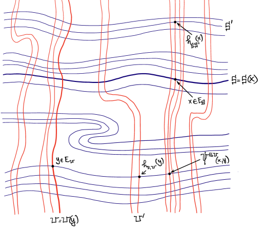
Figure 1. Illustration of Notation 2.6

Note that $\nu^{s}_{x}$ and $\nu^{u}_{y}$ are measures on entire streamlines, whereas $\nu_{{\mathfrak{s}}}$ and $\nu_{{\mathfrak{u}}}$ are restrictions of such measures to subsets of $R^{\pitchfork}$.

Definition 2.7 (Compatible tartan).

We say that the tartan $R=(R^{s},R^{u})$ is compatible (with the ambient measure $\mu$) if, for all stable and unstable fibers ${{\mathfrak{s}}}$ and ${{\mathfrak{u}}}$, the bijection $\psi^{{{\mathfrak{s}}},{{\mathfrak{u}}}}\colon E^{{\mathfrak{s}}}\times E^{{\mathfrak{u}}}\to R^{\pitchfork}$ is bi-measurable, and $\psi^{{{\mathfrak{s}}},{{\mathfrak{u}}}}_{*}\nu_{{{\mathfrak{s}}},{{\mathfrak{u}}}}=\mu|_{R^{\pitchfork}}$.

If $R$ is compatible and $A\subset R^{\pitchfork}$ is Borel, then using Fubini’s theorem in the product $E^{{\mathfrak{s}}}\times E^{{\mathfrak{u}}}$ and pushing forward to $R^{\pitchfork}$ we have, for any stable and unstable fibers ${{\mathfrak{s}}}$ and ${{\mathfrak{u}}}$,

$$\mu(A)=\int_{E^{{\mathfrak{s}}}}\nu_{{\mathfrak{u}}}(A^{{\mathfrak{u}}}(x))\,d\nu_{{\mathfrak{s}}}(x)=\int_{E^{{\mathfrak{u}}}}\nu_{{\mathfrak{s}}}(A^{{\mathfrak{s}}}(y))\,d\nu_{{\mathfrak{u}}}(y),$$ (1)

where $A^{{\mathfrak{u}}}(x)=\{y\in E^{{\mathfrak{u}}}\,:\,{{\mathfrak{u}}}(x)\pitchfork{{\mathfrak{s}}}(y)\in A\}$, and $A^{{\mathfrak{s}}}(y)=\{x\in E^{{\mathfrak{s}}}\,:\,{{\mathfrak{u}}}(x)\pitchfork{{\mathfrak{s}}}(y)\in A\}$.

Lemma 2.8 (Holonomy invariance).

Let $R$ be a compatible positive measure tartan, ${{\mathfrak{s}}}$ and ${{\mathfrak{s}}}^{\prime}$ be stable fibers of $R$, and $B\subset E^{{\mathfrak{s}}}$ be $\nu_{{\mathfrak{s}}}$-measurable. Then $B^{\prime}=h_{{{\mathfrak{s}}},{{\mathfrak{s}}}^{\prime}}(B)$ is $\nu_{{{\mathfrak{s}}}^{\prime}}$-measurable, and $\nu_{{{\mathfrak{s}}}^{\prime}}(B^{\prime})=\nu_{{\mathfrak{s}}}(B)$. The analogous statement holds for holonomies $h_{{{\mathfrak{u}}},{{\mathfrak{u}}}^{\prime}}$.

Proof.

Let ${{\mathfrak{u}}}$ be any unstable fiber. Then $\nu_{{\mathfrak{u}}}(E^{{\mathfrak{u}}})>0$ by (1) with $A=R^{\pitchfork}$.

Since $x$ and $h_{{{\mathfrak{s}}},{{\mathfrak{s}}}^{\prime}}(x)$ lie on the same unstable fiber ${{\mathfrak{u}}}(x)$ for all $x\in B$, we have $\psi^{{{\mathfrak{s}}},{{\mathfrak{u}}}}(B\times E^{{\mathfrak{u}}})=\psi^{{{\mathfrak{s}}}^{\prime},{{\mathfrak{u}}}}(B^{\prime}\times E^{{\mathfrak{u}}})$. Then $\nu_{{\mathfrak{s}}}$-measurability of $B$ implies $\mu$-measurability of $\psi^{{{\mathfrak{s}}},{{\mathfrak{u}}}}(B\times E^{{\mathfrak{u}}})=\psi^{{{\mathfrak{s}}}^{\prime},{{\mathfrak{u}}}}(B^{\prime}\times E^{{\mathfrak{u}}})$, and hence $\nu_{{{\mathfrak{s}}}^{\prime}}$-measurability of $B^{\prime}$.

Since $\mu(\psi^{{{\mathfrak{s}}},{{\mathfrak{u}}}}(B\times E^{{\mathfrak{u}}}))=\nu_{{\mathfrak{s}}}(B)\nu_{{\mathfrak{u}}}(E^{{\mathfrak{u}}})$ and $\mu(\psi^{{{\mathfrak{s}}}^{\prime},{{\mathfrak{u}}}}(B^{\prime}\times E^{{\mathfrak{u}}}))=\nu_{{{\mathfrak{s}}}^{\prime}}(B^{\prime})\nu_{{\mathfrak{u}}}(E^{{\mathfrak{u}}})$, the result follows. ∎

It is useful to have a version of (1) reflecting that fact that, in compatible tartans, the stream measures are the disintegration of the ambient measure onto fibers:

$$\mu(A)=\int_{E^{{\mathfrak{s}}}}\nu_{{{\mathfrak{u}}}(x)}(A\cap{{\mathfrak{u}}}(x))\,d\nu_{{\mathfrak{s}}}(x)=\int_{E^{{\mathfrak{u}}}}\nu_{{{\mathfrak{s}}}(y)}(A\cap{{\mathfrak{s}}}(y))\,d\nu_{{\mathfrak{u}}}(y).$$ (2)

This follows because

$$\nu_{{{\mathfrak{s}}}(y)}(A\cap{{\mathfrak{s}}}(y)) = \nu_{{\mathfrak{s}}}(h_{{{\mathfrak{s}}}(y),{{\mathfrak{s}}}}(A\cap{{\mathfrak{s}}}(y)))$$

$$= \nu_{{\mathfrak{s}}}(\{{{\mathfrak{u}}}(x)\pitchfork{{\mathfrak{s}}}\,:\,x\in A\cap{{\mathfrak{s}}}(y)\})$$

$$= \nu_{{\mathfrak{s}}}(\{x^{\prime}\in E^{{\mathfrak{s}}}\,:\,{{\mathfrak{u}}}(x^{\prime})\pitchfork{{\mathfrak{s}}}(y)\in A\})$$

$$= \nu_{{\mathfrak{s}}}(A^{{\mathfrak{s}}}(y)),$$

and likewise $\nu_{{{\mathfrak{u}}}(x)}(A\cap{{\mathfrak{u}}}(x))=\nu_{{\mathfrak{u}}}(A^{{\mathfrak{u}}}(x))$ for any $x\in E^{{\mathfrak{s}}}$.

Definitions 2.9 (Stable and unstable widths $w^{s}(R)$, $w^{u}(R)$).

Taking $B={{\mathfrak{s}}}\cap R^{\pitchfork}=E^{{\mathfrak{s}}}$ in Lemma 2.8, we see that if $R$ is compatible and positive measure then $\nu_{{\mathfrak{s}}}(E^{{\mathfrak{s}}})>0$ is independent of the stable fiber ${{\mathfrak{s}}}$; and similarly $\nu_{{\mathfrak{u}}}(E^{{\mathfrak{u}}})>0$ is independent of the unstable fiber ${{\mathfrak{u}}}$. We write $w^{s}(R)$ and $w^{u}(R)$ for these quantities (the stable and unstable widths of $R$), and note that $\mu(R^{\pitchfork})=w^{s}(R)\,w^{u}(R)$ by (1).

In order to be able to control the ambient measure $\mu$ from the product measures on tartans, it is clearly necessary for a full measure subset of $\Sigma$ to be covered by intersections of positive measure compatible tartans: this is condition (a) in the following definition. However, a corresponding topological condition, given by part (b) of the definition, is also useful: it follows from (a) if an additional regularity condition is imposed on tartans or on the turbulations. We return to this point in Section 5.

Definition 2.10 (Full turbulations).

We say that the transverse pair $({{\mathcal{T}}}^{s},\nu^{s})$ and $({{\mathcal{T}}}^{u},\nu^{u})$ is full if

1. There is a countable collection $R_{i}$ of (positive measure) compatible tartans with $\mu\left(\bigcup_{i}R_{i}^{\pitchfork}\right)=1$; and

2. for every non-empty open subset $U$ of $\Sigma$, there is a positive measure compatible tartan $R=(R^{s},R^{u})$ with $R^{s}\cup R^{u}\subset U$.

We are finally in a position to be able to define measurable pseudo-Anosov maps.

Definitions 2.11 (Image turbulation, measurable pseudo-Anosov turbulations, measurable pseudo-Anosov map, dilatation).

If $F\colon\Sigma\to\Sigma$ is a $\mu$-preserving homeomorphism, we write $F({{\mathcal{T}}},\nu)$ for the measured turbulation whose streamlines are $\{F(\ell)\,:\,\ell\in{{\mathcal{T}}}\}$, with measures $\nu_{F(\ell)}=F_{*}(\nu_{\ell})$.

A pair $({{\mathcal{T}}}^{s},\nu^{s}),({{\mathcal{T}}}^{u},\nu^{u})$ of measured turbulations on $\Sigma$ are measurable pseudo-Anosov turbulations if they are transverse, tame, full, and have dense streamlines.

A $\mu$-preserving homeomorphism $F\colon\Sigma\to\Sigma$ is measurable pseudo-Anosov if there is a pair $({{\mathcal{T}}}^{s},\nu^{s}),({{\mathcal{T}}}^{u},\nu^{u})$ of measurable pseudo-Anosov turbulations and a number $\lambda>1$, called the dilatation of $F$, such that $F({{\mathcal{T}}}^{s},\nu^{s})=({{\mathcal{T}}}^{s},\lambda\nu^{s})$ and $F({{\mathcal{T}}}^{u},\nu^{u})=({{\mathcal{T}}}^{u},\lambda^{-1}\nu^{u})$.

Note that the positions of $\lambda$ and $\lambda^{-1}$ here are not errors: they differ from those familiar in the definition of pseudo-Anosov maps since we are using measures along streamlines rather than transverse to them.

3. Subtartans

This short section describes some useful constructions of subtartans.

Definition 3.1 (Subtartan).

Let $R=(R^{s},R^{u})$ and $S=(S^{s},S^{u})$ be tartans. We say that $S$ is a subtartan of $R$ if every stable (respectively unstable) fiber of $S$ is contained in a stable (respectively unstable) fiber of $R$.

The simplest way to obtain a subtartan of $R$ is just to discard some of its fibers: if $S^{s}$ and $S^{u}$ are Borel subsets of $R^{s}$ and $R^{u}$ which are unions of fibers of $R$, then $S$ is a subtartan of $R$, which is clearly compatible if $R$ is.

Another construction is to take a rectangle bounded by segments of two stable and two unstable fibers of $R$, and to form a subtartan whose fibers are the intersections of fibers of $R$ with this rectangle.

Definition 3.2 ($R(x,y)$).

Let $R$ be a compatible tartan, and let $x,y\in R^{\pitchfork}$ lie on different stable and unstable fibers of $R$. Let $D$ be the closed disk bounded by the arcs $[x,{{\mathfrak{s}}}(x)\pitchfork{{\mathfrak{u}}}(y)]_{s}$, $[{{\mathfrak{s}}}(x)\pitchfork{{\mathfrak{u}}}(y),y]_{u}$, $[y,{{\mathfrak{s}}}(y)\pitchfork{{\mathfrak{u}}}(x)]_{s}$, and $[{{\mathfrak{s}}}(y)\pitchfork{{\mathfrak{u}}}(x),x]_{u}$. We define $R(x,y)$ to be the subtartan of $R$ whose stable and unstable fibers are the intersections of the stable and unstable fibers of $R$ with $D$.

It is easily seen that $R(x,y)$ is compatible, and that $w^{s}(R(x,y))=\nu_{{{\mathfrak{s}}}(x)}([x,{{\mathfrak{s}}}(x)\pitchfork{{\mathfrak{u}}}(y)]_{s})$ and $w^{u}(R(x,y))=\nu_{{{\mathfrak{u}}}(x)}([x,{{\mathfrak{s}}}(y)\pitchfork{{\mathfrak{u}}}(x)]_{u})$.

We can also construct subtartans which consist of all the fibers of $R$ which intersect given stable and unstable fibers in prescribed points. We start by defining how to trim a tartan to remove ‘loose’ segments of fibers.

Definition 3.3 ($\operatorname{trim}(R)$).

A tartan $R$ can be trimmed to yield a subtartan $\operatorname{trim}(R)$, by throwing away the ends of its fibers which contain no intersections. Each stable fiber ${{\mathfrak{s}}}$ of $R$ yields a stable fiber ${{\mathfrak{s}}}^{\prime}$ of $\operatorname{trim}(R)$, which is the minimal (open, closed, or half-open) subarc of ${{\mathfrak{s}}}$ which contains $E^{{\mathfrak{s}}}$, and analogously for unstable fibers.

Definition 3.4 ($R(I^{s},I^{u})$).

Let $R=(R^{s},R^{u})$ be a positive measure oriented compatible tartan, and let ${{\mathfrak{s}}}$ and ${{\mathfrak{u}}}$ be stable and unstable fibers of $R$.

For each $x\in E^{{\mathfrak{s}}}={{\mathfrak{s}}}\cap R^{\pitchfork}$, we denote by $\iota_{x}$ the initial (with respect to the given orientation of ${{\mathfrak{s}}}$) stream arc of ${{\mathfrak{s}}}$ with terminal endpoint $x$ (which may be open or closed at its initial point, according as ${{\mathfrak{s}}}$ is). Given a subinterval $I^{s}\subset[0,1]$, define $A^{s}(I^{s})\subset E^{{\mathfrak{s}}}$ by

$$A^{s}(I^{s})=\{x\in E^{{\mathfrak{s}}}\,:\,\nu_{{\mathfrak{s}}}(\iota_{x}\cap R^{\pitchfork})/w^{s}(R)\in I^{s}\}.$$

Likewise, if $I^{u}\subset[0,1]$ is a subinterval, we define a corresponding subset $A^{u}(I^{u})$ of $E^{{\mathfrak{u}}}$. We then define $R(I^{s},I^{u})$ by trimming the subtartan of $R$ whose stable fibers are ${{\mathfrak{s}}}(y)$ for $y\in A^{u}(I^{u})$, and whose unstable fibers are ${{\mathfrak{u}}}(x)$ for $x\in A^{s}(I^{s})$.

The definition is independent of the choice of fibers ${{\mathfrak{s}}}$ and ${{\mathfrak{u}}}$ by Lemma 2.8.

For example, $S=R([1/3,2/3],[1/3,2/3])$ is the ‘middle thirds’ subtartan of $R$, with $\mu(S^{\pitchfork})=\mu(R^{\pitchfork})/9$ (in contrast to the middle thirds Cantor set, here we retain the middle thirds of the stable and unstable fibers).

4. Density

Let $\alpha$ be an oriented stable or unstable stream arc with stream measure $\nu$. Then there is a stream metric $d_{\alpha}$ on $\alpha$ defined by $d_{\alpha}(x,y)=\nu([x,y]_{\alpha})$, with respect to which $\alpha$ is measure-preserving and orientation-preserving isometric to a finite interval $I$ in ${{\mathbb{R}}}$ with Lebesgue measure. In particular, we can apply the Lebesgue Density Theorem to stream arcs. In this section we present some consequences of the LDT which will be used later. In Lemma 4.3 we show that, for a compatible tartan $R$, the set $\operatorname{den}_{1}(R)$ of points of $R^{\pitchfork}$ which are (two-sided) density points of $R^{\pitchfork}$ along both stable and unstable fibers has full measure: moreover, the same is true for $\operatorname{den}_{2}(R)$, the set of points which are density points of $\operatorname{den}_{1}(R)$ along both fibers. Lemma 4.5 concerns points $x$ for which all small stream arcs with endpoint $x$ contain a high density of points of $R^{\pitchfork}$.

Notation 4.1.

Let $\varphi\colon I\to\alpha$ be such a measure-preserving and orientation-preserving isometry from an interval in ${{\mathbb{R}}}$ to an oriented stream arc. Pick some $x=\varphi({{\hat{x}}})\in\alpha$. If $a\in{{\mathbb{R}}}$ is small enough that ${{\hat{x}}}+a\in I$, then we denote by $x+a$ the point $\varphi({{\hat{x}}}+a)$ of $\alpha$.

When we write, for example, $[x,x+a]_{s}$ (respectively $[x,x+a]_{u}$), we mean the stream arc with endpoints $x$ and $x+a$ on the stable (respectively unstable) streamline through $x$: by construction, these arcs have stream measure $|a|$. In practice the orientation of $\alpha$ will be irrelevant, since the definitions which follow are invariant under $a\mapsto-a$.

Definition 4.2 ($\operatorname{den}_{k}(R)$).

Let $R$ be a compatible tartan. We define $\operatorname{den}_{k}(R)\subset R^{\pitchfork}$, the set of level $k$ density points of $R$, inductively for $k\geq 0$ by $\operatorname{den}_{0}(R)=R^{\pitchfork}$ and $\operatorname{den}_{k}(R)=\operatorname{den}_{k}^{s}(R)\cap\operatorname{den}_{k}^{u}(R)$, where

$$\operatorname{den}_{k}^{s/u}(R)=\{x\in\operatorname{den}_{k-1}(R)\,:\,\lim_{a\to 0}\frac{\nu^{s/u}_{x}([x,x+a]_{s/u}\cap\operatorname{den}_{k-1}(R))}{|a|}=1\}.$$

That is, an element $x$ of $\operatorname{den}_{k}(R)$ is an element of $R^{\pitchfork}$ which is a (2-sided) density point of $\operatorname{den}_{k-1}(R)$ along both ${{\mathfrak{s}}}(x)$ and ${{\mathfrak{u}}}(x)$.

Lemma 4.3.

Let $R$ be a compatible tartan. Then $\mu(\operatorname{den}_{k}(R))=\mu(R^{\pitchfork})$ for all $k\geq 0$.

Proof.

The proof is by induction on $k$, with the case $k=0$ vacuous. We can assume that $\mu(R^{\pitchfork})>0$.

Let ${{\mathfrak{u}}}$ be any unstable fiber of $R$, and define

$$T=\{y\in E^{{\mathfrak{u}}}\,:\,\nu_{{{\mathfrak{s}}}(y)}(\operatorname{den}_{k-1}(R)\cap{{\mathfrak{s}}}(y))=w^{s}(R)\}.$$

Since $\mu(R^{\pitchfork})-\mu(\operatorname{den}_{k-1}(R))=0$ by the inductive hypothesis, we have, by (2),

$$\int_{E^{{\mathfrak{u}}}}\left(w^{s}(R)-\nu_{{{\mathfrak{s}}}(y)}(\operatorname{den}_{k-1}(R)\cap{{\mathfrak{s}}}(y))\right)d\nu_{u}(y)=0,$$

and so $\nu_{{\mathfrak{u}}}(T)=\nu_{{\mathfrak{u}}}(E^{{\mathfrak{u}}})=w^{u}(R)$.

Let $y\in T$. Since $\operatorname{den}_{k-1}^{s}(R)\cap{{\mathfrak{s}}}(y)=\operatorname{den}_{k-1}^{s}(R)\cap E^{{{\mathfrak{s}}}(y)}$, we have

$$\operatorname{den}^{s}_{k}(R)\cap{{\mathfrak{s}}}(y)=\{x\in\operatorname{den}_{k-1}(R)\cap E^{{{\mathfrak{s}}}(y)}\,:\,\lim_{a\to 0}\frac{\nu^{s}_{x}([x,x+a]_{s}\cap(\operatorname{den}_{k-1}(R)\cap E^{{{\mathfrak{s}}}(y)}))}{|a|}=1\}.$$

Therefore, by the Lebesgue Density Theorem we have, writing $\ell$ for the streamline containing ${{\mathfrak{s}}}(y)$,

$$\nu_{{{\mathfrak{s}}}(y)}(\operatorname{den}_{k}^{s}(R)\cap{{\mathfrak{s}}}(y)) = \nu_{\ell}(\operatorname{den}_{k}^{s}(R)\cap{{\mathfrak{s}}}(y))=\nu_{\ell}(\operatorname{den}_{k-1}(R)\cap E^{{{\mathfrak{s}}}(y)})$$

$$= \nu_{{{\mathfrak{s}}}(y)}(\operatorname{den}_{k-1}(R)\cap{{\mathfrak{s}}}(y))=w^{s}(R).$$

It follows from (2) that

$$\mu(\operatorname{den}_{k}^{s}(R))=\int_{T}\nu_{{{\mathfrak{s}}}(y)}(\operatorname{den}_{k}^{s}(R)\cap{{\mathfrak{s}}}(y))d\nu_{{\mathfrak{u}}}(y)=w^{u}(R)w^{s}(R)=\mu(R^{\pitchfork}).$$

The same argument shows that $\mu(\operatorname{den}_{k}^{u}(R))=\mu(R^{\pitchfork})$, and the result follows. ∎

We now restrict to level 1 density points, and consider the set of points $x\in R^{\pitchfork}$ for which the density of intersections in all small stable and unstable stream arcs with endpoint $x$ is at least some prescribed value.

Definition 4.4 ($X_{\delta,\eta}(R)$).

Let $R$ be a compatible tartan. Given $\delta\in(0,1)$ and $\eta>0$, we define

$$X_{\delta,\eta}^{s/u}(R)=\{x\in R^{\pitchfork}\,:\,\nu_{x}^{s/u}([x,x+a]_{s/u}\cap R^{\pitchfork})\geq(1-\delta)|a|\text{ for all }a\in(-\eta,\eta)\},$$

and

$$X_{\delta,\eta}(R)=X_{\delta,\eta}^{s}(R)\cap X_{\delta,\eta}^{u}(R).$$

Lemma 4.5.

Let $R$ be a compatible tartan and $\delta\in(0,1)$. Then

$$\lim_{\eta\to 0}\mu(X_{\delta,\eta}(R))=\mu(R^{\pitchfork}).$$

Proof.

Note that if $\eta^{\prime}<\eta$ then $X_{\delta,\eta}(R)\subset X_{\delta,\eta^{\prime}}(R)$. Let

$$X_{\delta}(R)=\bigcup_{\eta>0}X_{\delta,\eta}(R)=\bigcup_{k\geq 1}X_{\delta,1/k}(R).$$

By continuity of measure, it suffices to show that $\mu(X_{\delta}(R))=\mu(R^{\pitchfork})$. This follows from Lemma 4.3 since $\operatorname{den}_{1}(R)\subset X_{\delta}(R)$, as can be easily shown. ∎

5. Positive measure tartans in open sets

Recall (Definition 2.10) that for a transverse pair of turbulations to be full, there are two requirements: first, that there is a countable collection of compatible tartans whose intersections cover a full measure subset of $\Sigma$; and second, that every non-empty open set contains a positive measure compatible tartan. We now discuss conditions which, combined with the first of these requirements, imply the second.

Let $U$ be a non-empty open subset of $\Sigma$. Since $\mu$ is OU we have $\mu(U)>0$, and hence, by the first requirement, there is a tartan $R$ with $\mu(R^{\pitchfork}\cap U)>0$. By Lemma 4.3 it follows that $\mu(\operatorname{den}_{2}(R)\cap U)>0$. Let $x\in\operatorname{den}_{2}(R)\cap U$.

For each $i\geq 1$, pick $a_{i}>0$ such that $[x,x+a_{i}]_{s}$ has diameter less than $1/i$. By definition of $\operatorname{den}_{2}(R)$, we can pick $y_{i}\in(x,x+a_{i}]_{s}\cap\operatorname{den}_{1}(R)$: moreover, we have $\nu_{{{\mathfrak{s}}}(x)}([x,y_{i}]_{s}\cap R^{\pitchfork})\geq\nu_{{{\mathfrak{s}}}(x)}([x,y_{i}]_{s}\cap\operatorname{den}_{1}(R))>0$.

Similarly, given $i$, for each $j\geq 1$ we pick $b_{i,j}>0$ such that $[y_{i},y_{i}+b_{i,j}]_{u}$ has diameter less than $1/j$. Since $y_{i}\in\operatorname{den}_{1}(R)$, we can pick $z_{i,j}\in(y_{i},y_{i}+b_{i,j}]_{u}\cap R^{\pitchfork}$; and $\nu_{{{\mathfrak{u}}}(y_{i})}([y_{i},z_{i,j}]_{u}\cap R^{\pitchfork})>0$.

For each $i$, the diameter of $[x,{{\mathfrak{s}}}(z_{i,j})\pitchfork{{\mathfrak{u}}}(x)]_{u}$ tends to zero as $j\to\infty$. For, given $\epsilon>0$, let $\delta>0$ be such that $[x,x+\delta]_{u}$ has diameter less than $\epsilon$, and let $w\in(x,x+\delta]_{u}\cap R^{\pitchfork}$ (such a point exists since $x\in\operatorname{den}_{2}^{u}(R)$). Let $j$ be large enough that $1/j$ is less than the diameter of $[y_{i},{{\mathfrak{u}}}(y_{i})\pitchfork{{\mathfrak{s}}}(w)]_{u}$: then $z_{i,j}\in[y_{i},{{\mathfrak{u}}}(y_{i})\pitchfork{{\mathfrak{s}}}(w)]_{u}$, so that ${{\mathfrak{s}}}(z_{i,j})\pitchfork{{\mathfrak{u}}}(x)\in[x,x+\delta]_{u}$ by Definitions 2.5(b).

Each $i\geq 1$ and $j\geq 1$ yields a compatible subtartan $R(x,z_{i,j})$ of $R$, with measure $\nu_{{{\mathfrak{s}}}(x)}([x,y_{i}]_{s}\cap R^{\pitchfork})\,\nu_{{{\mathfrak{u}}}(y_{i})}([y_{i},z_{i,j}]_{u}\cap R^{\pitchfork})>0$. If $i$ and $j$ are sufficiently large then the arcs $[x,y_{i}]_{s}$, $[y_{i},z_{i,j}]_{u}$, and $[x,{{\mathfrak{s}}}(z_{i,j})\pitchfork{{\mathfrak{u}}}(x)]_{u}$ are contained in $U$. Thus it suffices to show that we can choose $i$ and $j$ so that the remaining bounding arc $[z_{i,j},{{\mathfrak{s}}}(z_{i,j})\pitchfork{{\mathfrak{u}}}(x)]_{s}$ of $R(x,z_{i,j})$ is also contained in $U$. This is the step that requires an additional regularity condition on tartans or on the measured turbulations.

The simplest such condition just says that the result we need is true:

Definition 5.1 (Regular tartan).

We say that a tartan $R$ is regular if for all $x\in R^{\pitchfork}$ and all neighborhoods $U$ of $x$, there is some $\delta>0$ such that if $y\in{{\mathfrak{s}}}(x)\cap R^{\pitchfork}$ and $z\in{{\mathfrak{u}}}(x)\cap R^{\pitchfork}$ with $\nu_{{{\mathfrak{s}}}(x)}([x,y]_{s})<\delta$ and $\nu_{{{\mathfrak{u}}}(x)}([x,z]_{u})<\delta$, then $R(y,z)\subseteq U$ (that is, all of the fibers of $R(y,z)$ are contained in $U$).

A second condition which is perhaps more natural, in that it relates metric to stream measure within tartans, is:

Definition 5.2 (Bi-Lipschitz regular tartan).

We say that a tartan $R$ is (stable) bi-Lipschitz regular if there is a metric $d$ on $\Sigma$ compatible with its topology and a constant $K\geq 1$ such that whenever $x$ and $y$ lie on the same stable fiber of $R$, we have

$$\frac{1}{K}\,d(x,y)\leq\nu_{s}([x,y]_{s})\leq Kd(x,y).$$

A final condition is of interest because it can be expressed solely in terms of a single turbulation.

Definition 5.3 (Partial flowboxes).

A turbulation ${{\mathcal{T}}}$ has partial flowboxes if whenever

• $x$ and $y$ lie on the same streamline $\ell$ of ${{\mathcal{T}}}$, and

• there are arcs $\alpha_{x}$ and $\alpha_{y}$ in $\Sigma$, transverse to $\ell$ at $x$ and $y$, which contain transverse intersections with streamlines of ${{\mathcal{T}}}$ arbitrarily close to $x$ and $y$ on the same side of $\ell$,

then every neighborhood $U$ of the stream arc $[x,y]$ contains other stream arcs with endpoints on $\alpha_{x}$ and $\alpha_{y}$.

Lemma 5.4 (Conditions for positive measure tartans in open sets).

Let $({{\mathcal{T}}}^{s},\nu^{s})$ and $({{\mathcal{T}}}^{u},\nu^{u})$ be a transverse pair of measured turbulations which satisfy Definition 2.10(a), namely that there is a countable collection $R_{i}$ of compatible tartans with $\mu(\bigcup_{i}R_{i}^{\pitchfork})=1$. Then the pair also satisfies Definition 2.10(b), and so is full, if any of the following holds:

1. The tartans in Definition 2.10(a) can be chosen to be regular; or

2. The tartans in Definition 2.10(a) can be chosen to be bi-Lipschitz regular; or

3. The turbulations have partial flowboxes.

Proof.

Let $U$ be a non-empty open subset of $\Sigma$. As in the introduction to this section, we can find a tartan $R$ and a point $x\in R^{\pitchfork}\cap U$; and points $y\in{{\mathfrak{s}}}(x)$, $z\in{{\mathfrak{u}}}(y)$, and $w={{\mathfrak{s}}}(y)\pitchfork{{\mathfrak{u}}}(x)$ arbitrarily close to $x$ such that the subtartan $R(x,z)$ is compatible and has positive measure, and moreover $[x,y]_{s}$, $[x,w]_{u}$, and $[y,z]_{u}$ are contained in $U$. Thus it is only required to show that $y$, $z$, and $w$ can be chosen close enough to $x$ that $[z,w]_{s}$ is also contained in $U$.

This is clear if $R$ is regular: if $i$ and $j$ are sufficiently large, then the points $y$ and $w$ satisfy $\nu_{{{\mathfrak{s}}}(x)}([x,y]_{s})<\delta$ and $\nu_{{{\mathfrak{u}}}(x)}([x,w]_{u})<\delta$, where $\delta>0$ is provided by Definition 5.1.

If $R$ is stable bi-Lipschitz regular, then let $d$ be the metric and $K$ be the Lipschitz constant provided by Definition 5.2. Let $\epsilon>0$ be small enough that $B_{d}(x,2\epsilon)\subset U$, and let $\delta=\epsilon/K^{2}$. Pick $y$, $z$, and $w$ close enough to $x$ that $d(z,w)<\delta$ and $d(x,z)<\epsilon$. Then $\nu_{s}([z,w]_{s})<K\delta$, so that $\nu_{s}([z,v]_{s})<K\delta$ for all $v\in[z,w]_{s}$, and hence $d(z,v)<K^{2}\delta=\epsilon$ for all $v\in[z,w]_{s}$. Hence every $v\in[z,w]_{s}$ has $d(x,v)\leq d(x,z)+d(z,v)<2\epsilon$, and $[z,w]_{s}$ is contained in $U$ as required.

Finally, if the turbulation has partial flowboxes, then taking $\alpha_{x}$ and $\alpha_{y}$ to be ${{\mathfrak{u}}}(x)$ and ${{\mathfrak{u}}}(y)$ in Definition 5.3 immediately yields the result. ∎

Remark 5.5.

It is enough in Lemma 5.4(b) for each tartan to be either stable bi-Lipschitz regular or unstable bi-Lipschitz regular. Likewise, it is enough in (c) for just one of the turbulations to have partial flowboxes.

We finish this section with a first consequence of fullness.

Lemma 5.6.

Let $({{\mathcal{T}}}^{s},\nu^{s}),({{\mathcal{T}}}^{u},\nu^{u})$ be measurable pseudo-Anosov turbulations on $\Sigma$, and let $\ell_{s}$ and $\ell_{u}$ be stable and unstable streamlines. Then $\ell_{s}\cap\ell_{u}$ is dense in $\Sigma$.

Proof.

Suppose for a contradiction that there is a non-empty open subset $U$ of $\Sigma$ with $\ell_{s}\cap\ell_{u}\cap U=\emptyset$.

By fullness there is a positive measure compatible tartan $R$ contained in $U$. Any two stable and any two unstable fibers of $R$ contain stable arcs $s_{1},s_{2}$ and unstable arcs $u_{1},u_{2}$ which bound an open disk $V\subset U$. There are infinitely many such disks: choose one which does not contain an entire end of either $\ell_{s}$ or $\ell_{u}$ (recall that the streamlines are dense, but not necessarily bi-dense).

Since $\ell_{s}$ is dense in $\Sigma$, it contains a point $x$ of $V$. By the choice of $V$, the closure of the path component of $\ell_{s}\cap V$ containing $x$ is an arc $\alpha$ with endpoints in $u_{1}\cup u_{2}$. The endpoints of $\alpha$ can’t both lie on the same $u_{i}$, since then $\alpha$ and $u_{i}$ would bound a disk which $\ell_{u}$ cannot enter, contradicting the denseness of $\ell_{u}$. We conclude that there is an arc $\alpha\subset\overline{V}$ of $\ell_{s}$ with endpoints on $u_{1}$ and $u_{2}$.

Analogously, there is an arc $\beta\subset\overline{V}$ of $\ell_{u}$ with endpoints on $s_{1}$ and $s_{2}$. Then $\alpha$ and $\beta$ intersect in $V\subset U$, which is the required contradiction. ∎

6. Topological dynamics of measurable pseudo-Anosov maps

In this section we prove our main results about the topological dynamics of measurable pseudo-Anosov maps: that they are topologically transitive (Theorem 6.1) and that they have dense periodic points (Theorem 6.2). It follows [2] that they also exhibit sensitive dependence on initial conditions, and are therefore chaotic in the sense of Devaney [12].

Theorem 6.1.

Measurable pseudo-Anosov maps are topologically transitive.

Proof.

(See Figure 2.) Let $F\colon\Sigma\to\Sigma$ be measurable pseudo-Anosov with dilatation $\lambda>1$, and let $U$ and $V$ be non-empty open subsets of $\Sigma$. We need to show that there is some $n>0$ with $F^{n}(U)\cap V\not=\emptyset$.

By fullness, there is a positive measure compatible tartan $R$ contained in $U$. We write $S=R([0,1],[1/3,2/3])$, so that $w^{s}(S)=w^{s}(R)$ and $w^{u}(S)=w^{u}(R)/3$, and hence $\mu(S^{\pitchfork})=\mu(R^{\pitchfork})/3>0$.

Applying the Poincaré recurrence theorem to $F^{-1}$ yields a point $x_{0}\in S^{\pitchfork}$ and a sequence $n_{i}\to\infty$ such that $x_{i}=F^{-n_{i}}(x_{0})\in S^{\pitchfork}$ for all $i$.

Since the unstable streamline $\ell$ through $x_{0}$ is dense in $\Sigma$, it contains some point $y\in V$. Write $K=\nu^{u}_{\ell}([x_{0},y]_{\ell})$, and pick $i$ large enough that $\lambda^{n_{i}}w^{u}(R)/3>K$.

Let ${{\mathfrak{u}}}\subset U$ be the unstable fiber of $R$ which contains $x_{i}$. Then $x_{0}\in F^{n_{i}}({{\mathfrak{u}}})$, and each of the two components of $F^{n_{i}}({{\mathfrak{u}}})\setminus\{x_{0}\}$ has stream measure at least $\lambda^{n_{i}}w^{u}(R)/3>K$. Hence $y\in F^{n_{i}}({{\mathfrak{u}}})\subset F^{n_{i}}(U)$, so that $F^{n_{i}}(U)\cap V\not=\emptyset$ as required. ∎

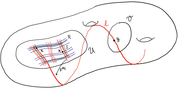
Figure 2. Proof of topological transitivity

The proof of density of periodic points is more challenging, and makes use of the density result of Lemma 4.5.

Theorem 6.2.

Measurable pseudo-Anosovs have dense periodic points.

Proof.

Let $F\colon\Sigma\to\Sigma$ be measurable pseudo-Anosov with dilatation $\lambda$, and let $U$ be a non-empty open subset of $\Sigma$. We need to show that there is a periodic point of $F$ in $U$.

By fullness, there is a positive measure compatible oriented tartan $R$ contained in $U$. We will show that there is a positive integer $n$ and an open rectangle $V\subset U$ such that (see Figure 3):

1. $\partial V$ is the union of two arcs $\alpha$ and $\alpha^{\prime}$ contained in stable fibers of $R$, and two arcs $\beta$ and $\beta^{\prime}$ contained in unstable fibers of $R$;

2. the $F^{n}$-images of these boundary arcs are also contained in stable and unstable fibers of $R$; and

3. $F^{n}(\beta)$ and $F^{n}(\beta^{\prime})$ both intersect both $\alpha$ and $\alpha^{\prime}$.

It follows that the fixed point index $\operatorname{index}(F^{n},V)$ of $V$ under $F^{n}$ is either $+1$ or $-1$ (depending on whether or not the orientations of the stable boundary arcs, and the unstable boundary arcs, are preserved by $F^{n}$), so that there is a fixed point of $F^{n}$ in $V\subset U$ as required.

Note that, if (V1) holds, then it is immediate from the definition of measurable pseudo-Anosov maps that the $F^{n}$-images of $\alpha$, $\alpha^{\prime}$, $\beta$, and $\beta^{\prime}$ are stream arcs, but that this is not enough: we need these images to be contained in fibers of $R$ so that we can control how they lie with respect to the original arcs.

Define subtartans $C$, $W$, $E$, $S$, and $N$ of $R$ (see Figure 3) by

$$C = R\,([1/3,2/3],[1/3,2/3]),$$

$$W = R\,([0,1/3],[1/3,2/3]),$$

$$E = R\,([2/3,1],[1/3,2/3]),$$

$$S = R\,([1/3,2/3],[0,1/3]),\text{ and}$$

$$N = R\,([1/3,2/3],[2/3,1]),$$

the Central, West, East, South, and North subtartans of $1/3$ the stable and unstable widths of $R$, where the stable streamlines of $R$ run from West to East and the unstable streamlines from South to North. We will construct the rectangle $V$ so that the unstable boundary arcs $\beta$ and $\beta^{\prime}$ lie in $W$ and $E$, while the image stable boundary arcs $F^{n}(\alpha)$ and $F^{n}(\alpha^{\prime})$ lie in $S$ and $N$ (not necessarily respectively in each case): this will ensure that (V3) holds.

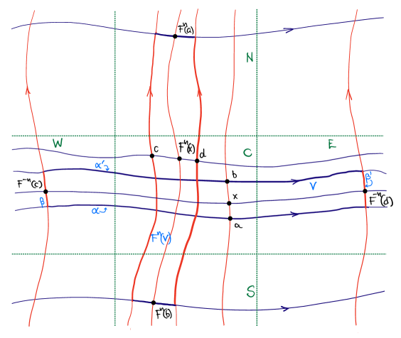
Figure 3. The rectangle $V$ and its image under $F^{n}$; the subdivision of $R$; the points $x$ and $F^{n}(x)$ and the construction of $a$, $b$, $c$, and $d$

Let

• $L$ be an upper bound on the stream measures of the fibers of $R$ (which exists by Definitions 2.5(c));

• $\delta\in(0,1)$ be such that $\delta<\min(w^{s}(R),w^{u}(R))/4\lambda L$;

• $\eta_{0}\in(0,L)$ be such that $\mu(X_{\delta,\eta_{0}}(C))>0$ (see Definition 4.4 and Lemma 4.5); and

• $n_{0}>0$ be such that $\eta_{0}\in[\lambda^{-n_{0}}L,\lambda^{-n_{0}+1}L)$.

By the Poincaré recurrence theorem applied to $X_{\delta,\eta_{0}}(C)$, there is an integer $n>n_{0}$ and a point $x\in X_{\delta,\eta_{0}}(C)$ such that $F^{n}(x)\in X_{\delta,\eta_{0}}(C)$.

Pick $\eta\in(\lambda^{-n}L,\lambda^{-n+1}L)$. Since $\eta_{0}\geq\lambda^{-n_{0}}L$ and $n>n_{0}$ we have $\eta<\eta_{0}$, so that $X_{\delta,\eta}(C)\supset X_{\delta,\eta_{0}}(C)$, and in particular $\{x,F^{n}(x)\}\subset X_{\delta,\eta}(C)$.

Note that $X_{\delta,\eta}(C)\subset C^{\pitchfork}$, so that $x$ and $F^{n}(x)$ are contained in both stable and unstable fibers of $C$, and hence in stable and unstable fibers of $R$.

We now use the point $x$ to build the rectangle $V$, starting with its stable boundary arcs $\alpha$ and $\alpha^{\prime}$: we will find points $a$ and $b$ of the unstable streamline of $x$, on either side of $x$ and within stream measure $\eta$ of $x$, which will lie on these arcs. The key properties are

• that $a,b\in C^{\pitchfork}\subset R^{\pitchfork}$, so that they lie on stable fibers of $R$; and

• that $F^{n}(a)$ and $F^{n}(b)$ lie in $S^{\pitchfork}\subset R^{\pitchfork}$ and $N^{\pitchfork}\subset R^{\pitchfork}$ (not necessarily respectively), so that (a) they also lie on stable fibers of $R$, and (b) $F^{n}(s)$ and $F^{n}(t)$ lie in $S$ and $N$, so that the image rectangle $F^{n}(V)$ stretches across $C$ in the unstable direction.

Let ${{\mathfrak{u}}}$ be the unstable fiber of $R$ through $F^{n}(x)$. We have $\nu^{u}_{F^{n}(x)}({{\mathfrak{u}}})\leq L$ by definition of $L$: since also $\lambda^{-n}L<\eta$, we have $F^{-n}({{\mathfrak{u}}})\subset(x-\eta,x+\eta)_{u}$.

We first find the point $a\in(x-\eta,x)_{u}$. By definition of $X_{\eta,\delta}(C)$, we have

$$\nu^{u}_{x}((x-\eta,x)_{u}\cap C^{\pitchfork})\geq(1-\delta)\eta.$$ (3)

We will assume that $F^{-n}$ sends ${{\mathfrak{u}}}$ into the unstable fiber through $x$ preserving the fiber orientation, so that $F^{-n}(S^{s}\cap{{\mathfrak{u}}})\subset(x-\eta,x)_{u}$: if it reverses fiber orientation, then we need only replace $S$ with $N$ (Figure 3 depicts the orientation-reversing case). Now

$$\nu^{u}_{x}(F^{-n}(S^{s}\cap{{\mathfrak{u}}}))=\lambda^{-n}\nu^{u}_{F^{n}(x)}(S^{s}\cap{{\mathfrak{u}}})=\lambda^{-n}w^{u}(S)>\lambda^{-n}w^{u}(R)/4>\delta\eta,$$ (4)

where the final inequality comes from $\delta<w^{u}(R)/4\lambda L$ and $\eta<\lambda^{-n+1}L$.

It follows from (3) and (4) that there is some $a\in(x-\eta,x)_{u}$ which lies in both $C^{\pitchfork}$ and in $F^{-n}(S^{s}\cap{{\mathfrak{u}}})$. That is, $a\in C^{\pitchfork}$ and $F^{n}(a)\in S^{\pitchfork}\supset S^{s}\cap{{\mathfrak{u}}}$ as required.

Applying the same argument to $(x,x+\eta)_{u}$ yields a point $b\in C^{\pitchfork}$ with $F^{n}(b)\in N^{\pitchfork}$ (or $S^{\pitchfork}$ if $F^{-n}$ reverses fiber orientation).

An exactly analogous argument applied to $(F^{n}(x)-\eta,F^{n}(x)+\eta)_{s}$ yields points $c,d\in C^{\pitchfork}\subset R^{\pitchfork}$ such that $F^{-n}(c)$ and $F^{-n}(d)$ lie in $W^{\pitchfork}\subset R^{\pitchfork}$ and $E^{\pitchfork}\subset R^{\pitchfork}$ (not necessarily respectively).

The rectangle $V$ whose boundary is contained in the stable fibers of $R$ through $a$ and $b$, and the unstable fibers of $R$ through $F^{-n}(c)$ and $F^{-n}(d)$ then has the required properties.

∎

7. Ergodicity

In this section we use a variant of the Hopf argument (see, for example, [1, 7, 8]) to prove ergodicity of measurable pseudo-Anosov maps. In classical uses of this argument, such as to prove the ergodicity of volume preserving Anosov diffeomorphisms, the main effort is in proving that the invariant foliations are absolutely continuous. This makes it possible to use a Fubini theorem to show that Birkhoff averages of $L^{1}$ functions are constant a.e. in charts. Since the manifold is connected and each point is contained in an open chart, this implies that the global Birkhoff average is constant a.e., yielding ergodicity.

In the case of measurable pseudo-Anosov maps, the compatibility conditions on a tartan $R$ allow a Fubini argument to show that Birkhoff averages are constant a.e. in $R^{\pitchfork}$. However, since tartans are not open sets we need an additional hypothesis connecting tartans in order to deal with the global averages.

Let $F\colon\Sigma\to\Sigma$ be measurable pseudo-Anosov with dilatation $\lambda>1$, and let $\phi\colon\Sigma\to{{\mathbb{R}}}$ be continuous. By Birkhoff’s ergodic theorem, the limits

$$\phi^{+}(x) = \lim_{n\to\infty}\frac{1}{n}\sum_{i=0}^{n-1}\phi(F^{i}(x))\text{ and }$$

$$\phi^{-}(x) = \lim_{n\to\infty}\frac{1}{n}\sum_{i=0}^{n-1}\phi(F^{-i}(x))$$

exist and are equal $\mu$-almost everywhere.

Since continuous functions are dense in $L^{1}$, using the converse of Birkhoff’s ergodic theorem, it suffices for ergodicity to show that for every continuous $\phi$, the functions $\phi^{+}$ and $\phi^{-}$ are constant almost everywhere.

Throughout this section we consider a fixed such function $\phi$.

Lemma 7.1.

Suppose that $x$ and $y$ lie in the same stable (respectively unstable) streamline $\ell$, and that $\phi^{+}(x)$ (respectively $\phi^{-}(x)$) exists. Then $\phi^{+}(y)$ (respectively $\phi^{-}(y)$) exists and is equal to $\phi^{+}(x)$ (respectively $\phi^{-}(x)$).

Proof.

If $x$ and $y$ lie in the same stable streamline $\ell$ with $\nu_{\ell}([x,y]_{s})=K$, then we have $\nu_{F^{i}(\ell)}([F^{i}(x),F^{i}(y)]_{s})=K/\lambda^{i}$.

Given $\epsilon>0$, let $N_{\epsilon}=\{(a,b)\in\Sigma\times\Sigma\,:\,|\phi(a)-\phi(b)|<\epsilon\}$, a neighborhood of the diagonal. By tameness there is a $\delta>0$ such that $(a,b)\in N_{\epsilon}$ whenever the stream measure of $[a,b]_{s}$ is less than $\delta$: therefore $|\phi(F^{i}(x))-\phi(F^{i}(y))|<\epsilon$ for all sufficiently large $i$. It follows that $\phi^{+}(y)=\phi^{+}(x)$ as required. The argument when $x$ and $y$ are on the same unstable streamline is analogous. ∎

Definitions 7.2 ($Z$, $\sim$).

Let

$$Z=\{x\in\Sigma\,:\,\phi^{+}(x)\text{ and }\phi^{-}(x)\text{ exist and are equal}\},$$

so that $\mu(Z)=1$ by Birkhoff’s ergodic theorem as noted above.

Let $x,y\in Z$. We write $x\sim y$ if there is a finite collection $\{\alpha_{1},\dots,\alpha_{k}\}$ of stream arcs with $x\in\alpha_{1}$ and $y\in\alpha_{k}$, such that $\alpha_{i}\cap\alpha_{i+1}$ contains a point $z_{i}\in Z$ for $1\leq i\leq k-1$.

$\sim$ is an equivalence relation on $Z$, and $\phi^{+}$ and $\phi^{-}$ are constant on equivalence classes. For, writing $z_{0}=x$ and $z_{k}=y$, we have for each $1\leq i\leq k$ that either $\phi^{+}(z_{i-1})=\phi^{+}(z_{i})$ or $\phi^{-}(z_{i-1})=\phi^{-}(z_{i})$ by Lemma 7.1; and hence $\phi^{\pm}(z_{i-1})=\phi^{\pm}(z_{i})$ since $z_{i-1},z_{i}\in Z$.

It follows that $F$ is ergodic if $\sim$ has a full measure equivalence class.

Lemma 7.3.

Let $R$ be a positive measure compatible tartan. Then $\phi^{+}=\phi^{-}$ is constant almost everywhere in $R^{\pitchfork}$.

Proof.

Let ${{\mathfrak{s}}}$ and ${{\mathfrak{u}}}$ be any stable and unstable fibers of $R$, and let $V=R^{\pitchfork}\cap Z$, a full measure subset of $R^{\pitchfork}$.

By (1),

$$\int_{E^{{\mathfrak{s}}}}\nu_{{\mathfrak{u}}}(E^{{\mathfrak{u}}})\,d\nu_{{\mathfrak{s}}}(x)=\mu(R^{\pitchfork})=\mu(V)=\int_{E^{{\mathfrak{s}}}}\nu_{{{\mathfrak{u}}}}(V^{{\mathfrak{u}}}(x))\,d\nu_{{\mathfrak{s}}}(x),$$

so that $W=\{x\in E^{{\mathfrak{s}}}\,:\,\nu_{{\mathfrak{u}}}(V^{{\mathfrak{u}}}(x))=\nu_{{\mathfrak{u}}}(E^{{\mathfrak{u}}})\}$ has full $\nu_{{\mathfrak{s}}}$-measure in $E^{{\mathfrak{s}}}$. Let $S$ be the subtartan of $R$ obtained by discarding the unstable fibers which don’t intersect $W$. Then $\mu(S^{\pitchfork})=\mu(R^{\pitchfork})$, and $\phi^{+}=\phi^{-}$ is constant on $S^{\pitchfork}\cap Z$, a full measure subset of $R^{\pitchfork}$. For if $a,a^{\prime}\in S^{\pitchfork}\cap Z$, then let $x,x^{\prime}\in W$ be such that $a\in{{\mathfrak{u}}}(x)$ and $a^{\prime}\in{{\mathfrak{u}}}(x^{\prime})$, and let $y\in V^{{\mathfrak{u}}}(x)\cap V^{{\mathfrak{u}}}(x^{\prime})$. Then the stream arcs $[a,{{\mathfrak{u}}}(x)\pitchfork{{\mathfrak{s}}}(y)]_{u}$, $[{{\mathfrak{u}}}(x)\pitchfork{{\mathfrak{s}}}(y),{{\mathfrak{u}}}(x^{\prime})\pitchfork{{\mathfrak{s}}}(y)]_{s}$, and $[{{\mathfrak{u}}}(x^{\prime})\pitchfork{{\mathfrak{s}}}(y),a^{\prime}]_{u}$ connect $a$ and $a^{\prime}$ and intersect at points of $V\subset Z$, so that $a\sim a^{\prime}$ as required (see Figure 4). ∎

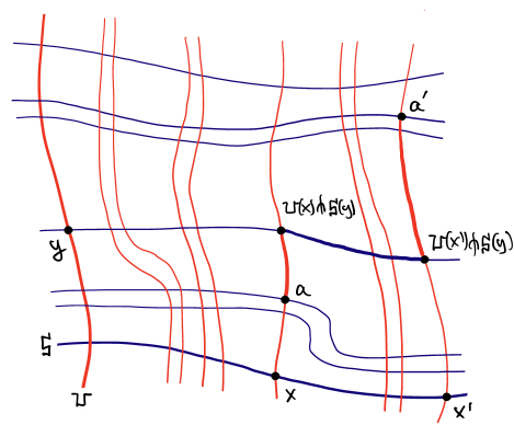
Figure 4. Stream arcs showing that $a\sim a^{\prime}$

In order to establish ergodicity, we need some means of relating the Birkhoff averages of $\phi$ on different positive measure tartans. The following is a natural, though strong, condition:

Definitions 7.4 (Tartan connection hypothesis).

We say that the measurable pseudo-Anosov turbulations $({{\mathcal{T}}}^{s},\nu^{s})$, $({{\mathcal{T}}}^{u},\nu^{u})$ satisfy the tartan connection hypothesis if for any compatible positive measure tartans $R$ and $S$, the stable streamlines containing fibers of $R$ intersect the unstable streamlines containing fibers of $S$ in positive measure.

Theorem 7.5.

If the turbulations of a measurable pseudo-Anosov map $F$ satisfy the tartan connection hypothesis, then $F$ is ergodic.

Proof.

Let $R_{i}$ be a countable collection of positive measure compatible tartans with $\mu(\bigcup_{i}R_{i}^{\pitchfork})=1$.

By Lemma 7.3 there are constants $\phi_{i}$ such that $\phi^{+}=\phi^{-}=\phi_{i}$ almost everywhere in $R_{i}^{\pitchfork}$, and it suffices to show that $\phi_{i}=\phi_{j}$ for all $i$ and $j$.

Given $i$ and $j$, let $S_{i}$ and $S_{j}$ be the positive measure compatible subtartans of $R_{i}$ and $R_{j}$ obtained by discarding the stable fibers of $R_{i}$ on which $\phi^{+}\not=\phi_{i}$ (or $\phi^{+}$ does not exist), and the unstable fibers of $R_{j}$ on which $\phi^{-}\not=\phi_{j}$ (or $\phi^{-}$ does not exist).

By the tartan connection hypothesis, the intersection $A$ of the union of the stable streamlines containing fibers of $S_{i}$ with the union of the unstable streamlines containing fibers of $S_{j}$ has positive measure, so that $\mu(A\cap Z)>0$. However if $a\in A\cap Z$ then $\phi^{+}(a)=\phi_{i}$ and $\phi^{-}(a)=\phi_{j}$ by Lemma 7.1. Since $a\in Z$ we have $\phi_{i}=\phi_{j}$ as required.

∎

Clearly Theorem 7.5 is also true under the weaker condition that for any compatible positive measure tartans $R$ and $S$, there is a chain $R=T_{0},T_{1},\dots,T_{k}=S$ of compatible tartans such that, for each $i$, the stable streamlines containing fibers of $T_{i}$ intersect the unstable streamlines containing fibers of $T_{i+1}$ in positive measure. This is worth mentioning because this weaker condition is in turn implied by the Tartan chain hypothesis: that for any compatible positive measure tartans $R$ and $S$, there is a chain as above such that $\mu(T_{i}^{\pitchfork}\cap T_{i+1}^{\pitchfork})>0$ for each $i$.

References

- [1] W. Ballmann, Lectures on spaces of nonpositive curvature, DMV Seminar, vol. 25, Birkhäuser Verlag, Basel, 1995, With an appendix by Misha Brin. MR 1377265
- [2] J. Banks, J. Brooks, G. Cairns, G. Davis, and P. Stacey, On Devaney’s definition of chaos, Amer. Math. Monthly 99 (1992), no. 4, 332–334. MR 1157223
- [3] E. Bedford, M. Lyubich, and J. Smillie, Polynomial diffeomorphisms of . IV. The measure of maximal entropy and laminar currents, Invent. Math. 112 (1993), no. 1, 77–125. MR 1207478
- [4] M. Bestvina and M. Handel, Train-tracks for surface homeomorphisms, Topology 34 (1995), no. 1, 109–140. MR 1308491
- [5] C. Bonatti and R. Langevin, Difféomorphismes de Smale des surfaces, Astérisque (1998), no. 250, viii+235, With the collaboration of E. Jeandenans. MR 1650926
- [6] P. Boyland, A. de Carvalho, and T. Hall, Unimodal measurable pseudo-Anosov maps, 2023, arXiv 2306.16059 [math.DS].
- [7] K. Burns, C. Pugh, M. Shub, and A. Wilkinson, Recent results about stable ergodicity, Smooth ergodic theory and its applications (Seattle, WA, 1999), Proc. Sympos. Pure Math., vol. 69, Amer. Math. Soc., Providence, RI, 2001, pp. 327–366. MR 1858538
- [8] Y. Coudène, The Hopf argument, J. Mod. Dyn. 1 (2007), no. 1, 147–153. MR 2261076
- [9] A. de Carvalho and T. Hall, Pruning theory and Thurston’s classification of surface homeomorphisms, J. Eur. Math. Soc. (JEMS) 3 (2001), no. 4, 287–333. MR 1866160
- [10] by same author, Unimodal generalized pseudo-Anosov maps, Geom. Topol. 8 (2004), 1127–1188. MR 2087080
- [11] A. de Carvalho and M. Paternain, Monotone quotients of surface diffeomorphisms, Math. Res. Lett. 10 (2003), no. 5-6, 603–619. MR 2024718
- [12] R. Devaney, An introduction to chaotic dynamical systems, CRC Press, Boca Raton, FL, 2022, Third edition [of 811850]. MR 4495651
- [13] A. Fathi, F. Laudenbach, and V. Poénaru, Travaux de Thurston sur les surfaces, Astérisque, vol. 66, Société Mathématique de France, Paris, 1979, Séminaire Orsay, With an English summary. MR 568308
- [14] J. Franks and M. Misiurewicz, Cycles for disk homeomorphisms and thick trees, Nielsen theory and dynamical systems (South Hadley, MA, 1992), Contemp. Math., vol. 152, Amer. Math. Soc., Providence, RI, 1993, pp. 69–139. MR 1243471
- [15] J. Los, Pseudo-Anosov maps and invariant train tracks in the disc: a finite algorithm, Proc. London Math. Soc. (3) 66 (1993), no. 2, 400–430. MR 1199073
- [16] M. Lyubich and Y. Minsky, Laminations in holomorphic dynamics, J. Differential Geom. 47 (1997), no. 1, 17–94. MR 1601430
- [17] J. Mello, Tight quotients of smale diffeomorphisms on surfaces, Ph.D. Thesis, Instituto Matemática e Estatística - Universidade de São Paulo, 2023.
- [18] M. Su, Measured solenoidal Riemann surfaces and holomorphic dynamics, J. Differential Geom. 47 (1997), no. 1, 170–195. MR 1601438
- [19] W. Thurston, On the geometry and dynamics of diffeomorphisms of surfaces, Bull. Amer. Math. Soc. (N.S.) 19 (1988), no. 2, 417–431. MR 956596