Spin Seebeck effect in the classical easy-axis antiferromagnetic chain

Abstract

By molecular dynamics simulations we study the spin Seebeck effect as a function of magnetic field in the prototype classical easy-axis antiferromagnetic chain, in the far-out of equilibrium as well as linear response regime. We find distinct behavior in the low field antiferromagnetic, middle field canted and high field ferromagnetic phase. In particular, in the open boundary system at low temperatures, we observe a divergence of the spin current in the spin-flop transition between the antiferromagnetic and canted phase, accompanied by a change of sign in the generated spin current by the temperature gradient. These results are corroborated by a simple spin-wave phenomenological analysis and simulations in the linear response regime. They shed light on the spin current sign change observed in experiments in bulk antiferromagnetic materials.

I Introduction

The generation and control of spin currents is a central topic in the field of spintronics review . In particular the spin Seebeck effect kikkawa , the generation of a spin current by a temperature gradient in a magnetic field, has been extensively experimentally and theoretically studied in a great variety of bulk magnetic systems as for instance, the ferrimagnetic YIG/Pt heterostructures, antiferromagnetic materials (e.g. Cr₂O₃, Fe₂O₃) and Van der Vaals 2D materials as the quasi-2D layered ferromagnets, Cr₂Si₂Te₆ and Cr₂Ge₂Te₆ (for an extensive reference review ). In particular, concerning easy-axis bulk antiferromagnetic materials, there is experimental wu ; li ; li2 ; yuan and theoretical rezende ; yamamoto ; reitz ; yamamoto2 interest and debate concerning the sign of the generated spin current kikkawa ; tserkovnyak .

In a different research domain, the physics of (quasi-) one dimensional magnetic systems, both classical and quantum, has been studied for years, starting with the Bethe ansatz solution of the antiferromagnetic spin-1/2 chain. In particular, the exotic physics of easy-axis antiferromagnetic spin chains mikeska and quantum spin liquid materials with topological spinon excitations has attracted great interest. The spin Seebeck effect in the spin-1/2 chains Sr₂CuO₃ with spinon and CuGeO₃ with triplon excitations has been studied experimentally hirobe ; triplon and rigorously evaluated theoretically psaroudaki in the easy-plane regime. Furthermore, the thermal transport of classical spin chains has been studied by numerical dynamics simulations savin and lately, the character of spin transport, ballistic, diffusive or anomalous, in classical and quantum (anti-) ferromagnetic chains attracts a great deal of attention (for a recent tour de force and references therein see google ).

The spin Seebeck effect has never been studied for the easy-axis classical antiferromagnetic spin chain and it makes sense to try to understand the physics of the effect in this prototype but realistic model. It allows us to clarify the relation of the sign of the induced spin current by a temperature gradient across the spin-flop transition occuring at a critical field and serves as a bridge between spintronics studies in bulk materials and model magnetic systems. Besides the academic interest, quasi-one dimensional compounds exist that can offer a platform for obtaining spin currents besides the bulk materials usually studied.

In the following, we first employ standard molecular dynamics (MD) simulations md to study the out of equilibrium spin current generation by a thermal current in a magnetic field. We find a sign reversal of the spin current at the critical field between the antiferromagnetic and canted ferromagnetic phase that we analyze by a simple spin-wave theory. The divergence of the induced current at the spin-flop transition, could be observed in large spin quasi-one dimensional spin chain compounds. The picture of the far-out of equilibrium spin Seebeck effect is corroborated by a simple spin-wave phenomenological model and simulations in the linear response regime.

II Model

The model we study is the classical antiferromagnetic Heisenberg chain with easy-axis anisotropy given by the Hamiltonian,

$$H=\sum_{l=1}^{L}J_{\perp}(S^{x}_{l}S^{x}_{l+1}+S^{y}_{l}S^{y}_{l+1})+\Delta S^{z}_{l}S^{z}_{l+1}-hS^{z}_{l},$$ (1)

where ${\bf S_{l}}$ is a unit vector with components $S^{x,y,z}_{l}$, $J_{\perp}>0$ is the in-plane and $\Delta>0$ the easy-axis exchange interactions with $\Delta>J_{\perp}$ and $h$ the magnetic field. We will use the common parametrization $S^{x}_{l}=\sin\theta_{l}\cdot\cos\phi_{l},S^{y}_{l}=\sin\theta_{l}\cdot\sin\phi_{l},S^{z}_{l}=\cos\theta_{l}$.

The spin dynamics is given by Landau-Lifshitz equations of motion,

$$\frac{d}{dt}{\bf S_{l}}={\bf S_{l}}\times\Big{(}-\frac{\partial H}{\partial{\bf S_{l}}}\Big{)}.$$ (2)

To study far-out of equilibrium transport, we use a straightforward numerical method, simulating the microscopic heat transfer by embedding the spin system between two Langevin thermostats at temperatures $T_{L},T_{R}$, realized by two Heisenberg chains of length $N_{L},N_{R}$. We apply the Heun method md to numerically integrate the stochastic version of the Landau-Lifshitz-Gilbert equation for magnetic systems,

$$(1+\alpha^{2})\frac{d}{dt}{\bf S_{l}}={\bf S_{l}}\times(\xi_{l}-\frac{\partial H}{\partial{\bf S_{l}}})-\alpha{\bf S_{l}}\Big{[}{\bf S_{l}}\times(\xi_{l}-\frac{\partial H}{\partial{\bf S_{l}}})\Big{]}$$ (3)

where $\alpha$ is a damping coefficient and $\xi_{l}$ a white Gaussian noise representing the thermostat at temperature $T$,

$$\langle\xi_{l}(t)\rangle=0,~{}~{}~{}\langle\xi_{l}(t_{1})\xi_{k}(t_{2})\rangle=2\alpha T\delta_{lk}\delta(t_{1}-t_{2}).$$

The spin $J^{S}$ and energy $J^{E}$ currents are given by the corresponding spin and energy continuity equations nz ; meisner ,

$$J^{S}=\sum_{l}J_{\perp}(S^{x}_{l}S^{y}_{l+1}-S^{y}_{l}S^{x}_{l+1})$$ (4)

$$J^{E}=-\sum_{l} J_{\perp}^{2}(S^{x}_{l-1}S^{z}_{l}S^{y}_{l+1}-S^{y}_{l-1}S^{z}_{l}S^{x}_{l+1})$$ (5)

$$- J_{\perp}\Delta S^{z}_{l-1}(S^{x}_{l}S^{y}_{l+1}-S^{y}_{l}S^{x}_{l+1})$$

$$- J_{\perp}\Delta(S^{x}_{l-1}S^{y}_{l}-S^{y}_{l-1}S^{x}_{l})S^{z}_{l+1}.$$

We first establish the phase diagram, in the zero temperature limit, by considering the high field region where $\theta_{l}=\theta,~{}~{}\phi_{l+1}-\phi_{l}=\pi$, obtaining by minimization of the energy,

$$E_{ferro}=-J_{\perp}\sin^{2}\theta+\Delta\cos^{2}\theta-h\cos\theta$$

$$z\equiv\cos\theta=\frac{h}{2(J_{\perp}+\Delta)}.$$ (6)

The critical field $h_{f}=2(J_{\perp}+\Delta)$ above which we have the ferromagnetic phase is obtained setting $z=1$. The critical magnetic field $h_{c}$, above which we have a canted ferromagnetic phase and below an antiferromagnetic one with $\theta_{l+1}-\theta_{l}=\pi$, is obtained by equating the energies of the two states

$$E_{\rm ferro}=E_{\rm afo}=-\Delta,~{}~{}~{}h_{c}=2\sqrt{\Delta^{2}-J_{\perp}^{2}}.$$

III MD results

In Fig.1 we show the ratio of the mean spin current $\langle J^{S}\rangle$ to the mean thermal current $\langle J^{Q}\rangle=\langle J^{E}\rangle-h\langle J^{S}\rangle$. The mean values, $\langle O\rangle=\frac{1}{L}\langle\sum_{l}O_{l}\rangle$, $O_{l}$ a local quantity, are obtained by averaging over about $10^{8}$ samples by sweeping over all lattice sites (we take, $N_{L}=N_{R}=L/2$). The thermal current is induced by setting the left (right) baths at different temperatures $T_{L}(T_{R})$, creating a constant temperature gradient along the chain. In the middle of the chain ($l=1,L$) the damping coefficient $\alpha$ and the white Gaussian noise $\xi_{l}$ are set equal to zero. The mean temperature is $T=0.02$, with up to $T_{L}=0.03,~{}~{}T_{R}=0.01$. Here, $J_{\perp}=0.8$ and we take $\Delta=1$ as the unit of energies and temperature, implying critical fields $h_{c}=1.2,~{}h_{f}=3.6$.

Concerning the numerical simulation, we find that the results are essentially independent of the temperature gradient within the accuracy of the simulation. The thermal gradient induces a thermal current, which in turn induces a spin current. Being a second order effect, the measured spin current shows rather large fluctuations in the data compared to the thermal current. Thus we use relatively large temperature gradients to improve the accuracy of the data. In the particular simulations we used as baths isotropic antiferromagnetic Heisenberg chains ($J_{\perp}=\Delta=1$) in zero magnetic field for which the energy-temperature relation is known. However, we found that the use of other baths, e.g. a ferromagnetic chain, or a phonon bath, does not qualitatively change the spin current-thermal current relation.

The most notable feature in the data in Fig.1 is the sharp reversal of the spin current at the spin-flop transition (to be dicussed later in the framework of a spin wave theory) and the size dependence indicating a diverging spin current in the zero temperature limit. In the low field antiferromagnetic phase the spin current is in the same direction as the thermal current, while in the ferromagnetic one it is opposite to the thermal current. Of course, as expected, reversing the direction of the magnetic field, reverses this relation. In the second part of the figure (below), we show the magnetic field dependence of the average magnetization $\langle S^{z}\rangle$ and nearest neighbor spin correlation $\langle S^{z}_{l+1}S^{z}_{l}\rangle$, clearly indicating the development of the three magnetic phases.

In Fig.2, we show the same quantities at a higher temperature where the transitions are smoothed out but the same features remain. Also, the finite size effects are reduced as well as the ratio of the spin to thermal current, in relation to the temperature increase.

In Fig.3 we show the field dependence of the spin and thermal conductivities separately. While the thermal current shows anomalies at the spin-flop and ferromagnetic transition, the spin current is clearly responsible for the sign changes and overall behavior shown in Fig.1.

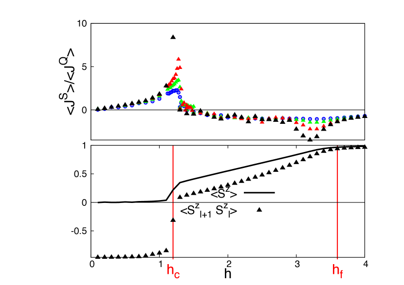
Figure 1: Ratio of spin to thermal current as a function of magnetic field for $J_{\perp}=0.8$. The mean $(T_{L}+T_{R})/2$ temperature is $T=0.02$ and the system sizes, $L=160~{}({\rm blue}),320~{}({\rm green}),640~{}({\rm red}),1280~{}({\rm black})$. Also shown below the mean magnetization (black line) and nearest neighbor spin-spin correlation (black triangles).

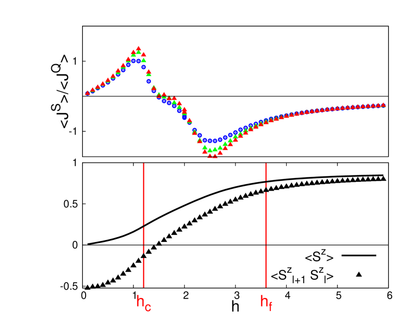
Figure 2: Ratio of spin to thermal current as a function of magnetic field for $J_{\perp}=0.8$. The mean $(T_{L}+T_{R})/2$ temperature is $T=0.2$ and the system sizes, $L=160~{}({\rm blue}),320~{}({\rm green}),640~{}({\rm red})$. Also shown below the mean magnetization (black line) and nearest neighbor spin-spin correlation (black triangles).

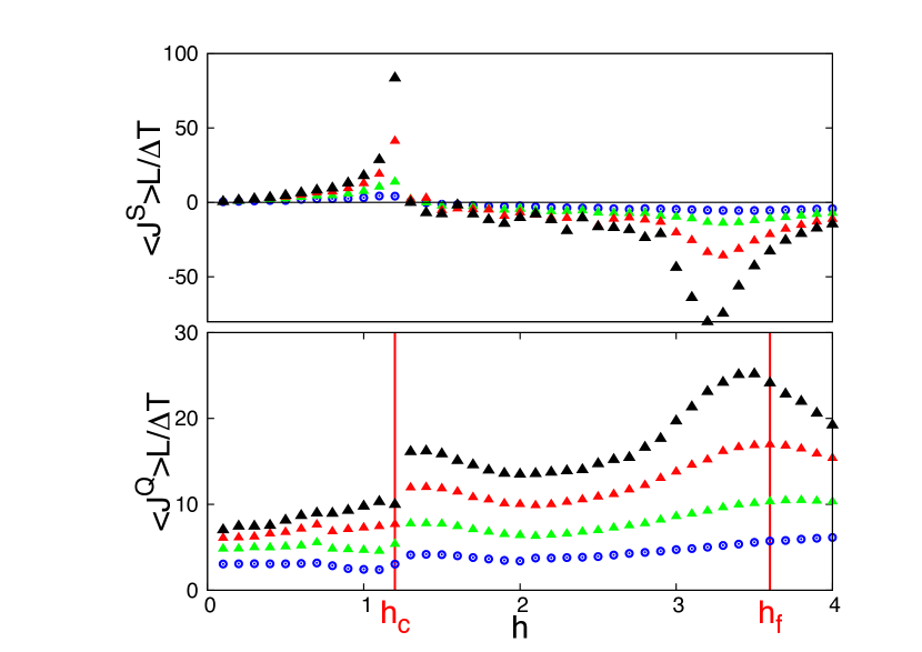
Figure 3: Spin and thermal conductivities as a function of magnetic field for $J_{\perp}=0.8$. The mean $(T_{L}+T_{R})/2$ temperature is $T=0.02$ and the system sizes, $L=160~{}({\rm blue}),320~{}({\rm green}),640~{}({\rm red}),1280~{}({\rm black})$.

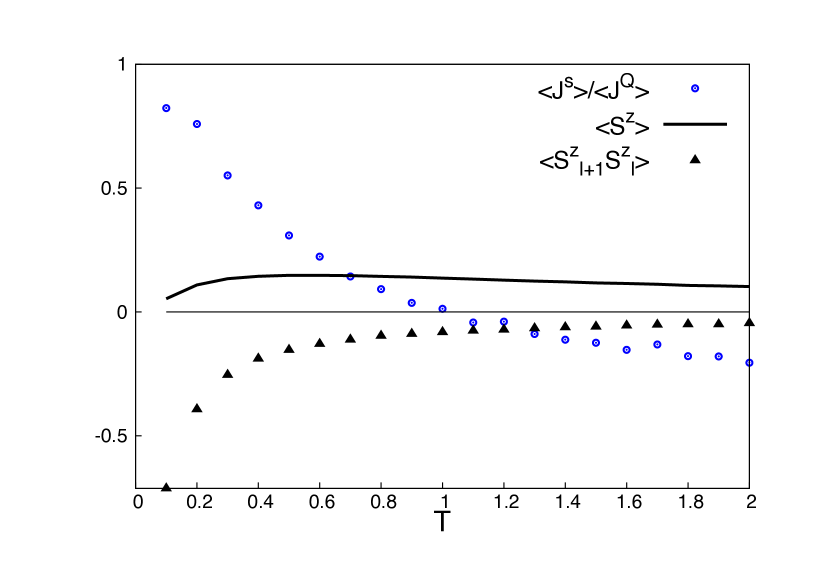
Figure 4: Ratio of spin to thermal current, magnetization and nearest neighbor correlations as a function of temperature for a magnetic field $h=0.8$ and $L=160$.

Finally in Fig.4 we show the temperature dependence of the spin Seebeck effect by the ratio $\langle J^{S}\rangle/\langle J^{Q}\rangle$ at $h=0.8$. In this field we are at the antiferromagnetic regime at low temperatures and the sign of the ratio is positive. Raising the temperature, the antiferromagnetic phase ”melts” with the appearance of an increasing number of domain walls, till a critical temperature $T\sim 1$ where we observe a change to a negative sign of the spin current, as in the ferromagnetic regime. To get an insight to this picture we show the temperature dependence of the uniform magnetization, rather small at this field and the decreasing nearest neighbor antiferromagnetic spin-spin correlations.

IV Spin-wave analysis

We can reach an understanding of the spin current sign reversal and divergence at the spin-flop transition, by considering a simple linear spin-wave theory. First, in the high field $|h|>h_{c}$ canted ferromagnetic phase, linearizing in $S^{x}_{l},S^{y}_{l}$ the equations of motion (2), we obtain,

$${\dot{S}^{x}}_{l} = -S^{y}_{l}(2\Delta z-h)+zJ_{\perp}(S^{y}_{l+1}+S^{y}_{l-1})$$

$${\dot{S}^{y}}_{l} = +S^{x}_{l}(2\Delta z-h)-zJ_{\perp}(S^{x}_{l+1}+S^{x}_{l-1})],$$

(the dot indicating the time derivative). With the substitution,

$$S^{x}_{l}\pm iS^{y}_{l}=ue^{i(ql-\omega_{\pm}t)},$$ (7)

we obtain the spin-wave spectrum,

$$\omega_{\pm}=\pm h\mp 2z(\Delta-J_{\perp}\cos q)$$

with positive eigenfrequencies,

$$\omega=h\Big{(}1-\frac{\Delta-J_{\perp}\cos q}{J_{\perp}+\Delta}\Big{)}.$$ (8)

Using (4,5,7), by substituting the values of $S^{x,y,z}_{l}$ for a spin-wave of wavevector $q$ we obtain for the spin and thermal current per unit length,

$$j^{s}_{q} = J_{\perp}u^{2}\sin q,$$

$$j^{\epsilon}_{q} = =-2J_{\perp}u^{2}(J_{\perp}\cos q-\Delta)z\cdot\sin q$$

$$u^{2} = 1-z^{2}$$

$$j^{Q}_{q} = j^{\epsilon}_{q}-hj^{s}_{q}$$

$$j^{Q}_{q} = -\Big{(}\frac{J_{\perp}(1+\cos q)}{\Delta+J_{\perp}}\Big{)}\cdot hj^{s}_{q}.$$

Thus we see that in the high field region, for $h>0$ the spin and thermal current have opposite sign, $j^{Q}_{q}>0$,  $j^{s}_{q}<0$ and of course for $h<0,~{}~{}j^{Q}_{q}>0,~{}~{}j^{s}_{q}>0$.

In the low field antiferromagnetic region, the equations of motion are,

$${\dot{S}^{x}}_{2l} = -S^{y}_{2l}(2\Delta S^{z}_{odd}-h)+S^{z}_{even}J_{\perp}(S^{y}_{2l+1}+S^{y}_{2l-1})$$

$${\dot{S}^{y}}_{2l} = +S^{x}_{2l}(2\Delta S^{z}_{odd}-h)-S^{z}_{even}J_{\perp}(S^{x}_{2l+1}+S^{x}_{2l-1})$$

$${\dot{S}^{x}}_{2l+1} = -S^{y}_{2l+1}(2\Delta S^{z}_{even}-h)+S^{z}_{odd}J_{\perp}(S^{y}_{2l}+S^{y}_{2l+2})$$

$${\dot{S}^{y}}_{2l+1} = +S^{x}_{2l+1}(2\Delta S^{z}_{even}-h)-S^{z}_{odd}J_{\perp}(S^{x}_{2l}+S^{x}_{2l+2}),$$

with $S^{z}_{odd,even}$ the alternating $S^{z}$ component at the odd, even sites. With the substitution,

$$S^{x}_{2l}\pm iS^{y}_{2l} = u_{\pm}e^{iq2l-\omega_{\pm}t}$$

$$S^{x}_{2l+1}\pm iS^{y}_{2l+1} = v_{\pm}e^{iq(2l+1)-\omega_{\pm}t}$$

and taking e.g. $S^{z}_{even}=+1,S^{z}_{odd}=-1$, we obtain the eigenvalue problem,

$$\begin{pmatrix}\pm(2\Delta+h)&\pm 2J_{\perp}\cos q\\ \mp 2J_{\perp}\cos q&\mp(2\Delta-h)\\ \end{pmatrix}\begin{pmatrix}u_{\pm}\\ v_{\pm}\end{pmatrix}=\omega_{\pm}\begin{pmatrix}u_{\pm}\\ v_{\pm}\end{pmatrix}$$

for the frequency spectrum,

$$\omega_{+\pm} = +h\pm 2\sqrt{\Delta^{2}-J_{\perp}^{2}\cos^{2}q}$$

$$\omega_{-\pm} = -h\pm 2\sqrt{\Delta^{2}-J_{\perp}^{2}\cos^{2}q}.$$ (9)

The positive frequency dispersions are, $\omega_{\pm+}=\pm h+h_{c}\sqrt{\frac{\Delta^{2}-J_{\perp}^{2}\cos^{2}q}{\Delta^{2}-J_{\perp}^{2}}}$. The lower frequency dispersion $\omega_{-+}$ vanishes as $q\rightarrow 0$ at the critical field $h_{c}$, signaling the spin-flop transition.

Setting $u_{-}-=\cos\phi,~{}v_{-}=\sin\phi,~{}\tan\phi=\frac{-\Delta-\sqrt{\Delta^{2}-J_{\perp}^{2}\cos^{2}q}}{J_{\perp}\cos q}$, we obtain the currents for the lower frequency dispersion,

$$j^{s}_{q} = -J_{\perp}u_{-}\cdot v_{-}\sin q=J_{\perp}\frac{J_{\perp}\cos q}{2\Delta}\sin q$$

$$j^{\epsilon}_{q} = \frac{1}{2}J_{\perp}^{2}(v_{-}^{2}-u_{-}^{2})\sin 2q$$

$$= \frac{1}{2}J_{\perp}^{2}\frac{\sqrt{\Delta^{2}-J_{\perp}^{2}\cos^{2}q}}{\Delta}\sin 2q$$

$$j^{Q}_{q} = j^{s}\cdot(h_{c}\cdot\sqrt{1+\frac{J_{\perp}^{2}(1-\cos^{2}q)}{\Delta^{2}-J_{\perp}^{2}}}-h),$$

$$j^{s}_{q}/j^{Q}_{q} > 0.$$ (10)

For the higher frequency dispersion $\omega_{++}$, setting, $u_{+}=\cos\phi,~{}v_{+}=\sin\phi,~{}\tan\phi=\frac{-\Delta+\sqrt{\Delta^{2}-J_{\perp}^{2}\cos^{2}q}}{J_{\perp}\cos q}$, we obtain the currents,

$$j^{s}_{q} = J_{\perp}u_{+}v_{+}\sin q=-J_{\perp}\frac{J_{\perp}\cos q}{2\Delta}\sin q$$

$$j^{\epsilon}_{q} = \frac{1}{2}J_{\perp}^{2}(u_{+}^{2}-v_{+}^{2})\sin 2q$$

$$= \frac{1}{2}J_{\perp}^{2}\frac{\sqrt{\Delta^{2}-J_{\perp}^{2}\cos^{2}q}}{\Delta}\sin 2q$$

$$j^{Q}_{q} = j^{s}\cdot(-2\sqrt{\Delta^{2}-J_{\perp}^{2}\cos^{2}q}-h)$$

$$j^{s}_{q}/j^{Q}_{q} < 0.$$

Thus, in the antiferromagnetic region, as observed in the simulations above, for $|h|<h_{c}$ the spin and thermal current of the dominating lower frequency dispersion spin-waves have the same sign $j^{s}_{q}/j^{Q}_{q}>0$. We can also get a hint on the diverging behavior of $\langle J^{s}\rangle/\langle J^{Q}\rangle$ for $h\rightarrow h_{c}$ from (10) as at low energies for $q\rightarrow 0$ this ratio diverges.

V ”Landauer” approach

The classical Heisenberg chain is a strongly interacting model with nonlinear equations of motion describing the spin dynamics. Therefore we expect normal transport coefficients savin e.g. finite thermal and spin conductivity, due to spin wave - spin wave scattering, although the anomalous behavior of spin transport in the isotropic Heisenberg model is presently in the focus of many theoretical studies google .

Nevertheless, for this open system with baths, we can obtain a heuristic description, shown in Fig.5, of the spin to thermal current ratio over the whole phase diagram by considering a phenomenological ”Landauer” type model. This can be justified by the low temperature in the simulations which implies a low spin wave density.

Assuming that spin and energy currents are emitted at the left-right leads at temperatures $T_{L,R},(\beta_{L,R}=1/T_{L,R})$, we obtain for $h<h_{c}$ (antiferromagnetic region),

$$\langle J^{S}\rangle = \sum_{\pm}\int_{0}^{+\pi/2}\frac{dq}{2\pi}(n_{\pm q}^{L}-n_{\pm q}^{R})j^{s}_{\pm q}$$

$$\langle J^{Q}\rangle = \sum_{\pm}\int_{0}^{+\pi/2}\frac{dq}{2\pi}(n_{\pm q}^{L}-n_{\pm q}^{R})j^{Q}_{\pm q}$$

summing the contributions over the positive frequency dispersions (9) with $n_{\pm q}^{L,R}=1/(e^{\beta_{L,R}\omega_{\pm q}}-1)$ (here we assume for simplicity a bosonic thermal distribution function). Similar expressions are obtained for $h>h_{c}$ summing over the positive frequency dispersion (8).

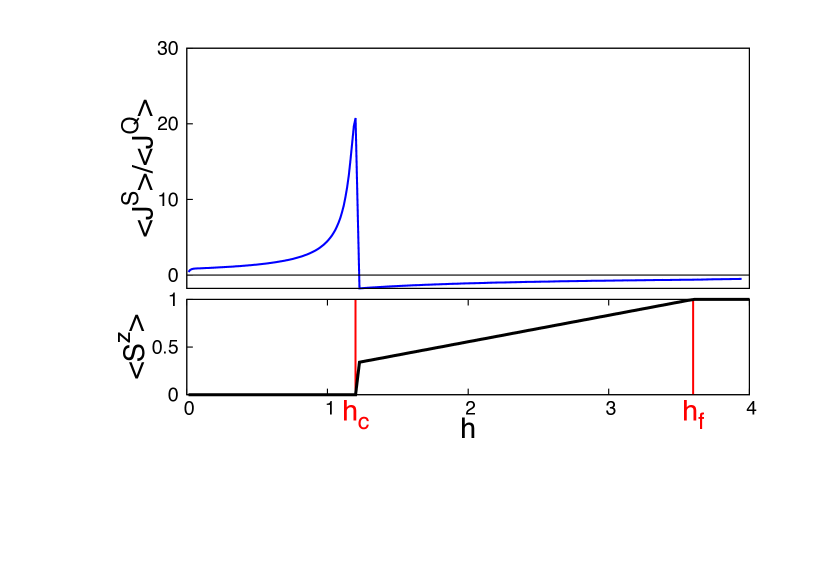
Figure 5: Spin current to thermal current ratio and magnetization as a function of magnetic field for $J_{\perp}=0.8$. Average temperature $T=(T_{L}+T_{R})/2=0.02$.

VI Linear response

Last but not least, in linear response the spin and thermal currents are related by transport coefficients $C_{ij}$,

$$\begin{pmatrix}J^{Q}\\ J^{S}\end{pmatrix}=\begin{pmatrix}C_{QQ}&C_{QS}\\ C_{SQ}&C_{SS}\end{pmatrix}\begin{pmatrix}-\nabla T\\ \nabla h\end{pmatrix}\,,$$ (11)

where $C_{QQ}=\kappa_{QQ}$ ($C_{ss}=\sigma_{ss}$) is the heat (spin) conductivity. The coefficients $C_{ij}$ are given by the thermal average of time-dependent current-current correlation functions in a closed system with periodic boundary conditions,

$$C_{i,j}=\frac{1}{L}\int_{0}^{\infty}dt\langle J^{i}(t)\cdot J^{j}(t=0)\rangle.$$

The time dependence is obtained by the same molecular dynamics procedure (3) after equilibrating the system at a given temperature and then switching-off the thermal noise. In Fig.6 we show two situations, (i) a system with no spin accumulation by setting $\nabla h=0$, relevant to an open system and (ii) a system with no spin current, $\langle J^{S}\rangle=0$ giving the spin Seebeck coefficient $S=\frac{\nabla h}{\nabla T}=\frac{C_{SQ}}{C_{SS}}$. For the open system, we find the same behavior of $\langle J^{S}\rangle/\langle J^{Q}\rangle$ as in the MD simulations.

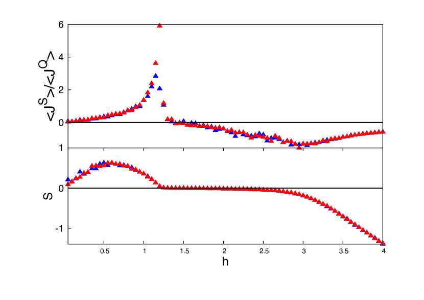
Figure 6: Linear response coefficients as a function of magnetic field at $J_{\perp}=0.8$ for $L=160$ (blue) and $L=320$ (red) at temperature $T=0.05$.

VII Conclusions

We have studied the spin Seebeck effect in the most simple prototype classical easy-axis magnetic chain model by molecular dynamics simulations and basic spin wave theory. We have found a sign change at the spin flop transition and clarified the role of spin wave excitations in the low field antiferromagnetic phase as well as in the high field ferromagnetic phase. This classical model could be realized experimentally in quasi-one dimensional large spin compounds but also provides a guide to the spin Seebeck effect studied over many years in bulk magnetic materials. The observations of this study should be extended to quantum spin systems, as the spin-1/2 easy-axis Heisenberg model, where the integrability of the model psaroudaki allows an exact evaluation of the spin Seebeck coefficient. The scope is to assess the potential of the large variety of spin chain materials for spintronic applications.

VIII Acknowledgments

X.Z. acknowledges stimulating discussions with Profs. C. Hess, P. van Loosdrecht and M. Valldor.

References

• (1) S. Maekawa, T. Kikkawa, H. Chudo, J. Ieda and E. Saitoh, J. of Appl. Phys., 133, 020902 (2023)
• (2) T. Kikkawa and E. Saitoh, Annu. Rev. Condens. Matter Phys. 14, 129 (2023)
• (3) S. M. Wu, W. Zhang, A. Kc, P. Borisov, J. E. Pearson, J. S. Jiang, D. Lederman, A. Hoffmann, and A. Bhattacharya, Phys. Rev. Lett. 116, 097204 (2016).
• (4) J. Li, C. B. Wilson, R. Cheng, M. Lohmann, M. Kavand, W. Yuan, M. Aldosary, N. Agladze, P. Wei, M. S. Sherwin, and J. Shi, Nature 578, 70 (2020).
• (5) J. Li, H. T. Simensen, D. Reitz, Q. Sun, W. Yuan, C. Li, Y. Tserkovnyak, A. Brataas, and J. Shi, Phys. Rev. Lett. 125, 217201 (2020).
• (6) Wei Yuan, Junxue Li, and Jing Shi, Appl. Phys. Lett. 117, 100501 (2020).
• (7) S. M. Rezende, R. L. Rodríguez-Suárez, and A. Azevedo, Phys. Rev. B 93, 014425 (2016).
• (8) Y. Yamamoto, M. Ichioka, and H. Adachi, Phys. Rev. B 100, 064419 (2019).
• (9) D. Reitz, J. Li, W. Yuan, J. Shi, and Y. Tserkovnyak, Phys. Rev. B 102, 020408(R) (2020).
• (10) Y. Yamamoto, M. Ichioka, and H. Adachi, Phys. Rev. B 105, 104417 (2022).
• (11) D. Reitz and Y. Tserkovnyak, arXiv:2307.02734.
• (12) H.J. Mikeska and M. Steiner, Advances in Physics, 40, 191 (1991).
• (13) D. Hirobe, M. Sato, T. Kawamata, Y. Shiomi, K. Uchida, R. Iguchi, Y. Koike, S. Maekawa, and E. Saitoh, Nat. Phys. 13, 30 (2017).
• (14) Y. Chen, M. Sato, Y. Tang, Y. Shiomi, K. Oyanagi, T. Masuda, Y. Nambu, M. Fujita and E. Saitoh, Nat. Comm. 12:5199 (2021).
• (15) C. Psaroudaki and X. Zotos, J. Stat. Mech. 063103 (2016).
• (16) A.V. Savin, G.P. Tsironis and X. Zotos, Phys. Rev. B72, 140402(R) (2005).
• (17) Google Quantum AI and Collaborators, arXiv:2306.09333.
• (18) J. L. Garcia-Palacios and F. J. Lazaro, Phys. Rev. B58, 14937 (1998)
• (19) F. Naef and X. Zotos, J. Phys. C 10, L183 (1998).
• (20) F. Heidrich-Meisner, A. Honecker, and W. Brenig Phys. Rev. B71, 184415 (2005).