Quasi-likelihood analysis for Student-Lévy regression

Abstract.

We consider the quasi-likelihood analysis for a linear regression model driven by a Student-$t$ Lévy process with constant scale and arbitrary degrees of freedom. The model is observed at a high frequency over an extending period, under which we can quantify how the sampling frequency affects estimation accuracy. In that setting, joint estimation of trend, scale, and degrees of freedom is a non-trivial problem. The bottleneck is that the Student-$t$ distribution is not closed under convolution, making it difficult to estimate all the parameters fully based on the high-frequency time scale. To efficiently deal with the intricate nature from both theoretical and computational points of view, we propose a two-step quasi-likelihood analysis: first, we make use of the Cauchy quasi-likelihood for estimating the regression-coefficient vector and the scale parameter; then, we construct the sequence of the unit-period cumulative residuals to estimate the remaining degrees of freedom. In particular, using full data in the first step causes a problem stemming from the small-time Cauchy approximation, showing the need for data thinning. Also presented is the implementation in a computer through the yuima package and some numerical examples.

1. Introduction

Suppose that we have a discrete-time sample $\{(X_{t_{j}},Y_{t_{j}})\}_{j=0}^{[nT_{n}]}$ with $t_{j}=j/n$ from the continuous-time (location) regression model

(1.1) $$Y_{t}=X_{t}\cdot\mu+\sigma J_{t},\qquad t\in[0,T_{n}],$$

where $X=(X_{t})$ is a càdlàg stochastic covariate process in $\mathbb{R}^{q}$ satisfying some regularity conditions, the dot denotes the inner product in $\mathbb{R}^{q}$, and $J=(J_{t})$ is a Lévy process such that the unit-time distribution

$$\mathcal{L}(J_{1})=t_{\nu}:=t_{\nu}(0,1),$$

where $t_{\nu}(\mu,\sigma)$ denotes the scaled Student-$t$ distribution with the density

(1.2) $$f(x;\mu,\sigma,\nu):=\frac{\Gamma(\frac{\nu+1}{2})}{\sigma\sqrt{\pi}\Gamma(\frac{\nu}{2})}\left\{1+\left(\frac{x-\mu}{\sigma}\right)^{2}\right\}^{-(\nu+1)/2}.$$

Our objective is to estimate the true value $\theta_{0}=(\mu_{0},\sigma_{0},\nu_{0})\in\Theta$ from $\{(X_{t_{j}},Y_{t_{j}})\}_{j=0}^{[nT_{n}]}$ when $T_{n}\to\infty$ for $n\to\infty$. We will write $h=h_{n}=1/n$ for the sampling step size. All the processes are defined on an underlying filtered probability space $(\Omega,\mathcal{F},(\mathcal{F}_{t})_{t\geq 0},P)$. The corresponding statistical model is indexed by the unknown parameter $\theta:=(\mu,\sigma,\nu)\in\Theta_{\mu}\times\Theta_{\sigma}\times\Theta_{\nu}=\Theta$. Throughout, we assume that $\Theta$ is a bounded convex domain in $\mathbb{R}^{q}+2$ such that its closure $\overline{\Theta}\subset\mathbb{R}^{q}\times(0,\infty)\times(0,\infty)$.

Since the Student-$t$ distribution is not closed under convolution, $\mathcal{L}(J_{h})$ for $h\neq 1$ is no longer Student-$t$-distributed. The exact likelihood function is given only through the Fourier inversion, resulting in the rather intractable expression: the characteristic function of $\mathcal{L}(J_{1})=t_{\nu}$ is given by

(1.3) $$\varphi_{J_{1},\nu}(u):=\frac{2^{1-\nu/2}}{\Gamma(\nu/2)}|u|^{\nu/2}K_{\nu/2}(|u|),\qquad u\in\mathbb{R},$$

hence $\mathcal{L}(J_{h})$ admits the Lebesgue density

$$x \mapsto\frac{1}{\pi}\int_{0}^{\infty}\cos(ux)\{\varphi_{J_{1},\nu}(u)\}^{h}du$$

$$=\frac{1}{\pi}\int_{0}^{\infty}\cos(ux)\left(\frac{2^{1-\nu/2}}{\Gamma(\nu/2)}u^{\nu/2}K_{\nu/2}(u)\right)^{h}du$$

(1.4) $$=\left(\frac{2^{1-\nu/2}}{\Gamma(\nu/2)}\right)^{h}\frac{1}{\pi}\int_{0}^{\infty}\cos(ux)u^{\nu h/2}\left(K_{\nu/2}(u)\right)^{h}du,$$

where $K_{\nu}(t)$ denotes the modified Bessel function of the second kind ($\nu\in\mathbb{R}$, $t>0$):

$$K_{\nu}(t)=\frac{1}{2}\int_{0}^{\infty}s^{\nu-1}\exp\left\{-\frac{t}{2}\left(s+\frac{1}{s}\right)\right\}ds.$$

Numerical integration can be unstable for very small $h$ and also for large $|x|$.

Previously, the thesis [21] studied in detail the local asymptotic behavior of the log-likelihood function with numerics for a sample-path generation about Student-$t$ Lévy process observed at high frequency. However, the degrees-of-freedom parameter $\nu$ was supposed to be known and to be greater than $1$ throughout.

In this paper, we propose the explicit two-stage estimation procedure:

1. First, in Section 2, we construct an estimator $(\hat{\mu}_{n},\hat{\sigma}_{n})$ of $(\mu,\sigma)$ based on the Cauchy quasi-likelihood;

2. Then, in Section 3, we make use of the Student-$t$ quasi-likelihood for construction of an estimator $\hat{\nu}_{n}$ of $\nu$, through the “unit-time” residual sequence

   $$\hat{\epsilon}_{i}:=\hat{\sigma}_{n}^{-1}\left(Y_{i}-Y_{i-1}-\hat{\mu}_{n}\cdot(X_{i}-X_{i-1})\right),$$

   for $i=1,\dots,[T_{n}]$, which is expected to be approximately i.i.d. $t_{\nu}$-distributed.

The important point is that we can asymptotically efficiently estimate $(\mu,\sigma)$, with effectively leaving $\nu$ unknown; under additional conditions, the least-squares estimator is asymptotically normal, but the associated efficiency loss can be significant (see Remark 2.5 below). We refer to [15] for the details of the corresponding LAN property. In our study, the rate of convergence of $(\hat{\mu}_{n},\hat{\sigma}_{n})$ in the first stage depends on how much data we use through the sequence $(B_{n})$ introduced later. Under suitable conditions, the two-stage procedure enables us to estimate $\nu_{0}$ as if we directly observe the latent unit-time noise sequence $(J_{i}-J_{i-1})_{i=1}^{[T_{n}]}$. We will present implementation in computer and some numerical experiments in Section 4. The proofs are gathered in Section 5.

Note that $X$ may be random and that $X$ and $J$ may be stochastically dependent on each other; in particular, $X$ may depend on $Y$. Our stepwise procedure with different time scales makes the optimization much easier than the joint estimation. Moreover, the proposed estimators $\hat{\sigma}_{n}$ and $\hat{\nu}_{n}$ are asymptotically independent (Theorem 3.2) while the maximum-likelihood estimators in the conventional i.i.d. and time-series settings are asymptotically correlated; see [13, Section 2.2] for details.

We will denote by $P_{\theta}$ the underlying probability measure for $(J,X,Y)$ associated with $\theta$, and by $E_{\theta}$ the expectation with respect to $P_{\theta}$. Unless otherwise mentioned, any asymptotics will be taken under $P:=P_{\theta_{0}}$ for $n\to\infty$. We will denote by $C$ a universal positive constant which may vary whenever it appears. The partial differentiation with respect to the variable $x$ will be denoted by $\partial_{x}$. The notation $a_{n}\lesssim b_{n}$ for positive sequences $(a_{n})$ and $(b_{n})$ means that $\limsup_{n}(a_{n}/b_{n})<\infty$.

2. Cauchy quasi-likelihood analysis

2.1. Construction and asymptotic results

By the expression (1.3) and the asymptotic property $K_{\nu}(z)\sim\sqrt{\pi/(2z)}e^{-z}$ for $z\to\infty$, the characteristic function of $h^{-1}J_{h}$ equals for $h\to 0$,

$$\left(E_{\theta}\left[\exp(iuh^{-1}J_{1})\right]\right)^{h} =(1+o(1))\big{|}u\nu^{-1/2}h^{-1}\big{|}^{\nu h/2}K_{\nu/2}\big{(}|uh^{-1}|\big{)}^{h}$$

$$=(1+o(1))\left(\sqrt{\frac{\pi h}{2|u|}}\exp\left(-h^{-1}|u|\right)(1+o(1))\right)^{h}$$

(2.1) $$\to\exp(-|u|).$$

This implies the weak convergence $h^{-1}J_{h}\xrightarrow{\mathcal{L}}t_{1}$ (the standard Cauchy distribution) as $h\to 0$, whatever the degrees of freedom $\nu_{0}>0$ is. It is therefore natural to construct the Cauchy quasi-(log-)likelihood which is defined as if the conditional distribution $Y_{t_{j}}|\{Y_{t_{j-1}}=y,\,X_{t_{j-1}},\,X_{t_{j}}\}$ under $P_{\theta}$ equals the Cauchy distribution with location $y+\mu\cdot(X_{t_{j}}-X_{t_{j-1}})$ and scale $h\sigma$; note that the conditional likelihood is misspecified unless $\nu_{0}=1$. There are both advantages and disadvantages: on the one hand, we can make an inference for $(\mu,\sigma)$ without knowing the value $\nu_{0}$, but on the other hand, the information of $\nu_{0}$ gets disappeared in the small-time limit.

Using the Cauchy quasi-likelihood is not free: we have to manage the Cauchy-approximation error for $\mathcal{L}(h^{-1}J_{h})$ in the mode of $L^{1}(dy)$-local-limit theorem. Since the approximation error accumulates for $T_{n}\to\infty$, using the whole sample $\{(X_{t_{j}},Y_{t_{j}})\}_{j=0}^{[nT_{n}]}$ may introduce too much error disrupting the Cauchy approximation; this will be seen from the proof of Theorem 2.2 below. Depending on the situation, we will need either to thin the sample or to control the speed of $T_{n}\to\infty$.

We consider the (possibly) partial observations over the part $[0,B_{n}]$ of the entire period $[0,T_{n}]$, where $(B_{n})$ is a positive sequence such that

(2.2) $$B_{n}\leq T_{n},\qquad n^{\epsilon^{\prime\prime}}\lesssim B_{n}\lesssim n^{1-\epsilon^{\prime}}$$

for some $\epsilon^{\prime},\epsilon^{\prime\prime}\in(0,1)$. We write the corresponding number of time points used as

(2.3) $$N_{n}=[nB_{n}].$$

Lemma 5.4 below implies that we cannot always take the whole sample (namely $B_{n}=T_{n}$) to manage the error of the local-Cauchy approximation. In other words, when one uses the whole sample for estimating $(\mu,\sigma)$, the condition (2.2) restricts the speed of $T_{n}\to\infty$ as $T_{n}=O(n^{1-\epsilon^{\prime}})$.

Write $a=(\mu,\sigma)$, $a_{0}=(\mu_{0},\sigma_{0})$, and $\Delta_{j}\xi=\xi_{t_{j}}-\xi_{t_{j-1}}$ for any process $\xi$. Let

$$\epsilon_{j}(a):=\frac{\Delta_{j}Y-\mu\cdot\Delta_{j}X}{h\sigma}.$$

Then, we introduce the Cauchy quasi-(log-)likelihood conditional on $X$:

$$\mathbb{H}_{1,n}(a) :=\sum_{j=1}^{N_{n}}\log\left\{\frac{1}{h\sigma}\phi_{1}\left(\frac{\Delta_{j}Y-\mu\cdot\Delta_{j}X}{h\sigma}\right)\right\}$$

$$=C_{n}-\sum_{j=1}^{N_{n}}\left\{\log\sigma+\log\left(1+\epsilon_{j}(a)^{2}\right)\right\},$$

where the term $C_{n}$ does not depend on $a$. We define the Cauchy quasi-maximum likelihood estimator (CQMLE for short) by any element

(2.4) $$\hat{a}_{n}:=(\hat{\mu}_{n},\hat{\sigma}_{n})\in\mathop{\rm argmax}_{a\in\overline{\Theta_{\mu}\times\Theta_{\sigma}}}\mathbb{H}_{1,n}(a).$$

We introduce the following regularity conditions on $X$.

Assumption 2.1.

For $X$, we can associate an $(\mathcal{F}_{t})$-adapted process $t\mapsto X^{\prime}_{t}$ having càdlàg sample paths, for which the following conditions hold for every $K>0$:

1. $\displaystyle{\sup_{t\geq 0}E\big{[}|X^{\prime}_{t}|^{K}\big{]}<\infty}$.

2. There exists a constant $c_{X}>0$ such that both

   (2.5) $$\sup_{n}\max_{j=1,\dots,[nT_{n}]}E\left[\left|\frac{1}{h^{c_{X}}}\left\{\frac{1}{h}\left(\Delta_{j}X-hX^{\prime}_{t_{j-1}}\right)\right\}\right|^{K}\right]<\infty$$

   and

   (2.6) $$\sup_{n}\max_{j=1,\dots,[nT_{n}]}\sup_{t_{j-1}\leq t\leq t_{j}}E\left[\left|\frac{1}{h^{c_{X}}}(X_{t}^{\prime}-X^{\prime}_{t_{j-1}})\right|^{K}\right]<\infty$$

   hold. Moreover,

   $$\limsup_{n}\max_{j=1,\dots,[nT_{n}]}E\left[\left|\sqrt{N_{n}}E\left.\left[\left\{\frac{1}{h}\left(\Delta_{j}X-hX^{\prime}_{t_{j-1}}\right)\right\}\,\frac{\partial\phi_{1}}{\phi_{1}}(\epsilon_{j})\right|\mathcal{F}_{t_{j-1}}\right]\right|^{K}\right]=0.$$

3. There exist a constant $c_{X}^{\prime}>0$ and a probability measure $\pi_{0}(dx)$ on the $q$-dimensional Borel space $(\mathbb{R}^{q},\mathcal{B}^{q})$ such that

   (2.7) $$\limsup_{M\to\infty}E\left[\sup_{a}\left|M^{c_{X}^{\prime}}\left(\frac{1}{M}\sum_{j=1}^{M}f(X^{\prime}_{t_{j-1}},a)-\int f(x^{\prime},a)\pi_{0}(dx^{\prime})\right)\right|^{K}\right]<\infty$$

   for every smooth function $f(x,a)$ such that $\sup_{a}\{|f(x,a)|\vee|\partial_{a}f(x,a)|\}\lesssim 1+|x|^{C}$.

4. The symmetric matrix $\displaystyle{S_{0}:=\int x^{\prime\,\otimes 2}\pi_{0}(dx^{\prime})}$ is positive-definite.

Since $\int f(x^{\prime})\pi_{0}(dx^{\prime})\leq\sup_{t\geq 0}E[f(X^{\prime}_{t})]$ for any continuous nonnegative $f$, we have $\int|x^{\prime}|^{K}\pi_{0}(dx^{\prime})$ for each $K>0$ and in particular $S_{0}$ is finite. One may think of $X_{t}=\int_{0}^{t}X^{\prime}_{s}ds$, where sample paths of $X^{\prime}$ may have certain discontinuity: alternatively, we could consider a bounded non-random $X^{\prime}$ satisfying a certain uniform-continuity condition over each period $[i-1,i)$, but the resulting regularity conditions will look complicated.

Let

$$\Delta_{a,n} :=\frac{1}{\sqrt{N_{n}}}\partial_{a}\mathbb{H}_{1,n}(a_{0}),$$

(2.8) $$\Gamma_{a,0} :={\rm diag}\left(\frac{1}{2\sigma_{0}^{2}}\,S_{0},~{}\frac{1}{2\sigma_{0}^{2}}\right).$$

The main result of this section is the following.

Theorem 2.2.

Under (2.2) and Assumption 2.1, we have the asymptotic normality

(2.9) $$\hat{u}_{a,n}:=\sqrt{N_{n}}(\hat{a}_{n}-a_{0})=\Gamma_{a,0}^{-1}\Delta_{a,n}+o_{p}(1)\xrightarrow{\mathcal{L}}N\left(0,\,\Gamma_{a,0}^{-1}\right)$$

and the polynomial-type tail-probability estimate:

(2.10) $$\forall L>0,\quad\sup_{r>0}\sup_{n}P\left[|\hat{u}_{a,n}|>r\right]r^{L}<\infty.$$

We have the variance-stabilizing transform for $\sigma$: $\sqrt{N_{n}/2}(\log\hat{\sigma}_{n}-\log\sigma_{0})\xrightarrow{\mathcal{L}}N_{1}(0,1)$.

Remark 2.3.

Making use of sample in over $[0,B_{n}]\subset[0,T_{n}]$ is not essential. It is possible to use, for example, only sample over $\bigcup_{k\geq 1}[2k-2,2k-1)$. Also, we could consider the case where $B_{n}\equiv B$ for some fixed $B>0$, meaning that for estimating $(\mu,\sigma)$ we only use a sample over the fixed period $[0,B]$. In that case, if $X$ is truly random, under suitable conditions on the underlying filtration $(\mathcal{F}_{t})$, the asymptotic distribution of $\sqrt{n}(\hat{a}_{n}-a_{0})$ is mixed-normal with the random asymptotic covariance depending on a sample path $(X_{t})_{t\in[0,B]}$. See also Remark 3.3, [6], [7], and [24] for related results.

Remark 2.4.

Since high-frequency data over each fixed period is enough to consistently estimate $(\mu,\sigma)$, one may think of a parameter-varying (randomized parameter) setting: if $\mu$ and $\sigma$ may vary along $i$, say $i\mapsto(\mu_{i},\sigma_{i})$ for the $i$th period $[i-1,i)$ and if they are all to be estimated from $\{(X_{t_{j}},Y_{t_{j}})\}_{j\geq 1:\,jh\in[i-1,i)}$, then the model setup invokes the classical Neyman-Scott problem [27]; if $\{(\mu_{i},\sigma_{i})\}_{i\geq 1}$ is an unobserved i.i.d. sequence of random vectors, then the model becomes a (partially) random-effect one. The latter would be of interest in the context of the population approach.

Remark 2.5 (Least-squares estimator).

Let $\nu_{0}>2$. We can rewrite (1.1) as

$$Y_{t}=X_{t}\cdot\mu+\sigma^{\prime}Z_{t}$$

with $\sigma^{\prime}:=\sigma/\sqrt{\nu-2}$ and the Lévy process $Z_{t}:=\sqrt{\nu-2}\,J_{t}$ such that $E[Z_{1}]=0$ and ${\rm var}[Z_{1}]=1$. In this case, under suitable conditions, we can apply the least-squares method for estimating $(\mu,\sigma^{\prime})$ and deduce its asymptotic normality at rate $\sqrt{T_{n}}$.

Remark 2.6.

The claims in Theorem 2.2 hold for any local-Cauchy $J$ satisfying the local limit theorem Lemma 5.4. In particular, the model (1.1) with $J$ replaced by the generalized hyperbolic Lévy process (except for the variance gamma one) could be handled analogously; see [24, Section 2.1.2] for related information.

2.2. Covariate process

Let us briefly discuss how to verify Assumption 2.1 for $X_{t}=(X_{1,t},X_{2,t})\in\mathbb{R}^{q_{1}}\times\mathbb{R}^{q_{2}}$ ($q=q_{1}+q_{2}$) of the form

(2.11) $$t\mapsto X_{k,t}=\int_{0}^{t}X^{\prime}_{k,s}ds,\qquad k=1,2,$$

where $t\mapsto X^{\prime}_{1,t}$ is bounded and periodic with unknown period and where $t\mapsto X^{\prime}_{2,t}$ is an ergodic process, with $(X^{\prime}_{1},X^{\prime}_{2})$ being independent of the Student-$t$ noise process $J$. Our model may be used for analyzing time series data observed at high frequency exhibiting a seasonality [28].

To be specific, we will focus on the non-random derivative of

(2.12) $$X_{1,t}=\big{(}\cos(\tau_{1}t),\sin(\tau_{1}t),\dots,\cos(\tau_{M}t),\sin(\tau_{M}t)\big{)}$$

for $X^{\prime}_{1}$ ($q_{1}=2M$ in this case) and a $q_{2}$-dimensional ergodic diffusion for $X^{\prime}_{2}$:

(2.13) $$dX^{\prime}_{2,t}=A(X^{\prime}_{2,t})dw_{t}+B(X^{\prime}_{2,t})dt.$$

Here, $\tau_{m}>0$ are given constants, the unknown coefficients $A$ and $B$ are assumed to be globally Lipschitz with $A^{\otimes 2}$ being uniformly elliptic, and $w$ is a standard Wiener process. We assume that $X^{\prime}_{2}$ is exponentially ergodic in the sense that

$$\sup_{t\geq 0}\sup_{f:\,|f|\leq g}\left|\int f(y)(P_{t}(x,dy)-\pi_{0}(dy))\right|\lesssim g(x)e^{-\kappa t}$$

for some $\kappa>0$; see [17], [16], and also [23, Section 5] for sufficient conditions. Further, though not essential, we assume that $X^{\prime}_{2}$ is strictly stationary. For $X^{\prime}_{1}$, we may get rid of some of the components from the beginning, such as $X_{1,t}=(\cos(5t),\sin(t))$. With these settings, we will verify Assumption 2.1.

For (1) and (2), we can look at $X_{1}$ and $X_{2}$ separately. The conditions obviously hold for $X_{1}$ of (2.12). As for $X_{2}$ of (2.13), several existing criteria exist. (1) can be verified through the Lyapunov-function criteria, see [22, Theorem 2.2] and [17, Lemma 3.3]. Then, all the conditions in (2) hold since $\sqrt{N_{n}}\,h\lesssim n^{-\epsilon^{\prime}/2}\to 0$ ($c_{X}=1/2$) and since both

$$\frac{1}{h\sqrt{h}}\left(\Delta_{j}X_{2}-hX^{\prime}_{2,t_{j-1}}\right)=\frac{1}{h}\int_{t_{j-1}}^{t_{j}}\frac{1}{\sqrt{h}}(X^{\prime}_{2,s}-X^{\prime}_{2,t_{j-1}})ds$$

and

$$\frac{1}{\sqrt{h}}(X^{\prime}_{2,t}-X^{\prime}_{2,t_{j-1}})=\frac{1}{\sqrt{h}}\int_{t_{j-1}}^{t}A(X_{s})dw_{s}+\sqrt{h}\,\frac{1}{h}\int_{t_{j-1}}^{t}B(X_{s})ds$$

are $L^{K}(P)$-bounded for any $K>0$ in the sense of the first two displays in Assumption 2.1(2).

Turning to (3), we recall the decomposition (5.14). Following the flow therein in reverse, we can replace Assumption 2.1(3) by

$$\limsup_{n}E\left[\sup_{a}\left|N_{n}^{c^{\prime}_{X}}\left(\frac{1}{hN_{n}}\int_{0}^{hN_{n}}f(X^{\prime}_{t},a)dt-\int f(x^{\prime},a)\pi_{0}(dx^{\prime})\right)\right|^{K}\right]<\infty.$$

Let $\tau>0$ denote the (unknown) period of $X^{\prime}_{1}$ and write $M_{n}=\max\{i\geq 1:\,i\tau\leq hN_{n}\}$. Then, $M_{n}\uparrow\infty$ as $n\to\infty$ and $\frac{1}{hN_{n}}\int_{0}^{hN_{n}}f(X^{\prime}_{t},a)dt=\frac{1}{hN_{n}}\int_{0}^{\tau M_{n}}f(X^{\prime}_{t},a)dt+\frac{1}{hN_{n}}\int_{\tau M_{n}}^{hN_{n}}f(X^{\prime}_{t},a)dt$. The second term can be bounded by a constant multiple of $(hN_{n})^{-1}(1+|X^{\prime}_{t}|^{C})\lesssim n^{-\epsilon^{\prime\prime}}(1+|X^{\prime}_{t}|^{C})$ (recall (2.2)). Letting $c^{\prime}_{X}$ sufficiently small, we only need to look at the first one, say $V_{n}(a)$, which can be expressed as follows:

$$V_{n}(a) =\frac{1}{hN_{n}}\sum_{m=1}^{M_{n}}\int_{(m-1)\tau}^{m\tau}f(X^{\prime}_{t},a)dt$$

$$=\frac{\tau M_{n}}{hN_{n}}\frac{1}{M_{n}}\sum_{m=1}^{M_{n}}\frac{1}{\tau}\int_{0}^{\tau}f\left((X^{\prime}_{1,(m-1)\tau+t},X^{\prime}_{2,(m-1)\tau+t}),a\right)dt$$

$$=\frac{\tau M_{n}}{hN_{n}}\frac{1}{M_{n}}\sum_{m=1}^{M_{n}}\frac{1}{\tau}\int_{0}^{\tau}f\left((X^{\prime}_{1,t},X^{\prime}_{2,(m-1)\tau+t}),a\right)dt$$

$$=:\frac{\tau M_{n}}{hN_{n}}\,\frac{1}{M_{n}}\sum_{m=1}^{M_{n}}G_{m}(a).$$

Since $E[G_{m}(a)]=\int f(x^{\prime},a)\pi_{0}(dx^{\prime})$ for each $a$, centering the summands yields

$$V_{n}(a)-\int f(x^{\prime},a)\pi_{0}(dx^{\prime}) =\left(\frac{\tau M_{n}}{hN_{n}}-1\right)\,\frac{1}{M_{n}}\sum_{m=1}^{M_{n}}G_{m}(a)+\frac{1}{M_{n}}\sum_{m=1}^{M_{n}}\left(G_{m}(a)-E[G_{m}(a)]\right)$$

Note that $|\frac{\tau M_{n}}{hN_{n}}-1|=O((hN_{n})^{-1})=O(n^{-\epsilon^{\prime\prime}})$ and that $\{(X^{\prime}_{1,(m-1)\tau+t},X^{\prime}_{2,(m-1)\tau+t})_{t\in[0,\tau]}\}_{m\geq 1}$ is strictly stationary and exponentially ergodic. Therefore, following the same line as in the proof of [23, Lemma 4.3], we obtain

(2.14) $$\limsup_{n}E\left[\sup_{a}\left|n^{c_{3}}\left(\frac{1}{M_{n}}\sum_{m=1}^{M_{n}}G_{m}(a)-\int f(x^{\prime},a)\pi_{0}(dx^{\prime})\right)\right|^{K}\right]<\infty$$

for a sufficiently small constant $c_{3}>0$, hence Assumption 2.1(3).

3. Student quasi-likelihood analysis

Taking over the setting in Section 2, we now turn to the estimation of the degrees of freedom $\nu$ from $\{(X_{t_{j}},Y_{t_{j}})\}_{j=0}^{[nT_{n}]}$. Suppose that Assumption 2.1 and (2.2) hold, so that we have (2.10) by Theorem 2.2. Throughout this section, we assume that $N_{n}$ is sufficiently large relative to $T_{n}$:

(3.1) $$\frac{T_{n}}{N_{n}}=\frac{T_{n}}{[nB_{n}]}\to 0.$$

3.1. Construction and asymptotics

Define the unit-time residual sequence

$$\hat{\epsilon}_{i}:=\hat{\sigma}_{n}^{-1}\left(Y_{i}-Y_{i-1}-\hat{\mu}_{n}\cdot(X_{i}-X_{i-1})\right),$$

for $i=1,\dots,[T_{n}]$. Let $\epsilon_{i}:=J_{i}-J_{i-1}$, so that $\epsilon_{1},\epsilon_{2},\dots\sim\text{i.i.d.}~{}t_{\nu}$. We will estimate $\nu$ based on the maximum-likelihood function as if $\hat{\epsilon}_{1},\dots,\hat{\epsilon}_{[T_{n}]}$ are observed $t_{\nu}$-i.i.d. samples: we consider the explicit Student quasi-likelihood function

(3.2) $$\mathbb{H}_{2,n}(\nu)=\sum_{i=1}^{[T_{n}]}\rho(\hat{\epsilon}_{i};\nu),$$

where $\rho(\epsilon;\nu):=\log f(\epsilon;0,1,\nu)$ (recall the notation (1.2)):

$$f(\epsilon;0,1,\nu)=\frac{\Gamma(\frac{\nu+1}{2})}{\sqrt{\pi}\Gamma(\frac{\nu}{2})}\left(1+\epsilon^{2}\right)^{-(\nu+1)/2}.$$

Then, we define the Student-$t$ quasi-likelihood estimator ($t$-QMLE for short) of $\nu$ by any element

$$\hat{\nu}_{n}\in\mathop{\rm argmax}_{\nu\in\overline{\Theta}_{\nu}}\mathbb{H}_{2,n}(\nu).$$

We have

$$\mathbb{H}_{2,n}(\nu)=\sum_{i=1}^{[T_{n}]}\left(-\frac{1}{2}\log\pi+\log\Gamma\left(\frac{\nu+1}{2}\right)-\log\Gamma\left(\frac{\nu}{2}\right)-\frac{\nu+1}{2}\log\left(1+\hat{\epsilon}_{i}^{2}\right)\right).$$

Let $\psi(x):=\partial\log\Gamma(x)$, the digamma function, and then $\psi_{1}:=\partial\psi$, the trigamma function. By the integral representation $\partial^{m}\psi(x)=(-1)^{m+1}\int_{0}^{\infty}s^{m}e^{-xs}(1-e^{-s})^{-1}ds$ for $m\in\mathbb{N}$ (see [1, 6.4.1]), hence $\partial\psi_{1}(x)<0$ for $x>0$. From this fact and the last expression for $\mathbb{H}_{2,n}(\nu)$, we obtain

(3.3) $$-\partial_{\nu}^{2}\mathbb{H}_{2,n}(\nu)=\frac{[T_{n}]}{4}\left(\psi_{1}\left(\frac{\nu}{2}\right)-\psi_{1}\left(\frac{\nu+1}{2}\right)\right)>0$$

for any $\nu>0$, hence $-\mathbb{H}_{2,n}$ is a.s. convex on $(0,\infty)$.

Let

$$\Delta_{\nu,n} :=\frac{1}{\sqrt{T_{n}}}\sum_{i=1}^{[T_{n}]}\partial_{\nu}\rho(\epsilon_{i};\nu_{0}),$$

(3.4) $$\Gamma_{\nu,0} :=\frac{1}{4}\left(\psi_{1}\left(\frac{\nu_{0}}{2}\right)-\psi_{1}\left(\frac{\nu_{0}+1}{2}\right)\right).$$

We have $\Gamma_{\nu,0}>0$ by (3.3). The next result shows that we can estimate $\nu_{0}$ directly as if we observe $(\epsilon_{i})$.

Theorem 3.1.

Under (2.2), Assumption 2.1, and (3.1), we have the polynomial-type tail-probability estimate:

(3.5) $$\forall L>0,\quad\sup_{r>0}\sup_{n}P\left[|\hat{u}_{\nu,n}|>r\right]r^{L}<\infty,$$

and the asymptotic normality:

(3.6) $$\hat{u}_{\nu,n}:=\sqrt{T_{n}}(\hat{\nu}_{n}-\nu_{0})=\Gamma_{\nu,0}^{-1}\Delta_{\nu,n}+o_{p}(1)\xrightarrow{\mathcal{L}}N\left(0,\,\Gamma_{\nu,0}^{-1}\right).$$

The maximum-likelihood estimation of $\nu_{0}$ can become more unstable for a larger value of $\nu_{0}$. The Fisher information $\Gamma_{\nu,0}$ quickly decreases to $0$ as $\nu_{0}$ increases: the asymptotic variance $\Gamma_{\nu,0}^{-1}$ equals about $1.22$, $5.63$, $13.8$, $25.9$, and $41.9$ for $\nu_{0}=1,2,3,4$, and $5$, respectively. The damping speed becomes even faster in the case of conventional parametrization. See, for example, [13, Section 2.2] and the references therein.

An asymptotically efficient estimation of $\nu$ based on the full high-frequency sample $\{(X_{t_{j}},Y_{t_{j}})\}_{j=0}^{[nT_{n}]}$ is a non-trivial problem; indeed, we do not know even whether or not $\sqrt{T_{n}}$ is the optimal rate of convergence for estimating $\nu_{0}$. We do not address it in this paper.

3.2. Joint asymptotic normality

Having Theorems 2.2 and 3.1 in hand, we consider the question of the joint asymptotic normality of $\hat{a}_{n}$ and $\hat{\nu}_{n}$.

Recall that we are given the underlying filtration $(\mathcal{F}_{t})_{t\geq 0}$. From the proofs of Theorems 2.2 and 3.1, we can write $(\hat{u}_{a,n},\hat{u}_{\nu,n})=M_{n}+o_{p}(1)$ with

$$M_{n}=\frac{1}{\sqrt{T_{n}}}\sum_{i=1}^{[T_{n}]}G_{i}=\frac{1}{\sqrt{T_{n}}}\sum_{i=1}^{[T_{n}]}\left(G_{a,i},\,G_{\nu,i}\right)$$

for a martingale difference $G_{\nu,i}=\partial_{\nu}\rho(\epsilon_{i};\nu_{0})\in\mathbb{R}^{q+1}$ with respect to $(\mathcal{F}_{i})_{i\in\mathbb{Z}_{+}}$ and

$$G_{a,i} :=\sqrt{\frac{T_{n}}{N_{n}}}\,I(i\leq[B_{n}])\sum_{j\in A_{i}}\psi_{a,ij},$$

where $A_{i}:=\{k\in\mathbb{N}:\,(i-1)\,n<k\leq i\,n\}$ and $\psi_{a,ij}=\psi_{a,ij}(a_{0}):=-\partial_{a}\left\{\log\sigma+\log\left(1+\epsilon_{j}(a)^{2}\right)\right\}|_{a=a_{0}}$. It will be seen in the proof of Lemma 5.3 that $T_{n}^{-1/2}\sum_{i=1}^{[T_{n}]}E[G_{a,i}|\mathcal{F}_{t_{j-1}}]=o_{p}(1)$. Hence, $M_{n}$ is a partial sum of the approximate martingale difference array with respect to $(\mathcal{F}_{i})_{i\in\mathbb{Z}_{+}}$.

The Lyapunov condition holds for $M_{n}$. To deduce the first-order asymptotic behavior of $M_{n}$, we need to look at the convergence in probability of the matrix-valued quadratic characteristic:

$$[M]_{n} :=\frac{1}{T_{n}}\sum_{i=1}^{[T_{n}]}\begin{pmatrix}G_{a,i}^{\otimes 2}&G_{a,i}G_{\nu,i}\\ \text{sym.}&G_{\nu,i}^{2}\end{pmatrix},$$

which explicitly depends on $\theta_{0}=(a_{0},\nu_{0})$; among others, we refer to [31, Chapter VII.8] for the related basic facts. By Theorems 2.2 and 3.1, it remains to manage the cross-covariation part of $[M]_{n}$.

To that end, we further assume

(3.7) $$\frac{B_{n}}{T_{n}}\to 0.$$

By Lemmas 5.2 and 5.6 in Section 5.1, for any $K>0$,

$$\max_{1\leq i\leq[T_{n}]}\max_{1\leq j\leq[nT_{n}]}E\left[|\psi_{a,ij}|^{K}+|G_{\nu,i}|^{K}\right]+\max_{1\leq i\leq[T_{n}]}E\left[\left|\frac{1}{\sqrt{n}}\sum_{j\in A_{i}}\psi_{a,ij}\right|^{K}\right]=O(1).$$

This estimate leads to

$$\frac{1}{T_{n}}\sum_{i=1}^{[T_{n}]}G_{\nu,i}G_{a,i}=\sqrt{\frac{B_{n}}{T_{n}}}\,\frac{1}{B_{n}}\sum_{i=1}^{[B_{n}]}G_{\nu,i}\sqrt{\frac{1}{n}}\sum_{j\in A_{i}}\psi_{a,ij}=O_{p}\left(\sqrt{\frac{B_{n}}{T_{n}}}\right)=o_{p}(1).$$

Thus, the additional condition (3.7) approximately quantifies how much data we should discard to make the estimators $\hat{a}_{n}$ and $\hat{\nu}_{n}$ independent.

Under Assumption 2.1,

$$\hat{S}_{n} :=\frac{1}{N_{n}}\sum_{j=1}^{N_{n}}\left(\frac{1}{h}\Delta_{j}X\right)^{\otimes 2}$$

$$=\frac{1}{N_{n}}\sum_{j=1}^{N_{n}}\left\{\left(\frac{1}{h}\Delta_{j}X-X^{\prime}_{t_{j-1}}\right)+X^{\prime}_{t_{j-1}}\right\}^{\otimes 2}$$

$$=\frac{1}{N_{n}}\sum_{j=1}^{N_{n}}(X^{\prime}_{t_{j-1}})^{\otimes 2}+o_{p}(1)\xrightarrow{p}S_{0},\qquad n\to\infty,$$

Recalling the notation (2.8) and (3.4), we introduce

$$\hat{\Gamma}_{a,n} :={\rm diag}\left(\frac{1}{2\hat{\sigma}_{n}^{2}}\,\hat{S}_{n},~{}\frac{1}{2\hat{\sigma}_{n}^{2}}\right),$$

$$\hat{\Gamma}_{\nu,n} :=\frac{1}{4}\left(\psi_{1}\left(\frac{\hat{\nu}_{n}}{2}\right)-\psi_{1}\left(\frac{\hat{\nu}_{n}+1}{2}\right)\right).$$

Obviously we have $(\hat{\Gamma}_{a,n},\hat{\Gamma}_{a,n})\xrightarrow{p}(\Gamma_{a,0},\Gamma_{\nu,0})$, which combined with (2.9) and (3.6) leads to the joint asymptotic normality:

Theorem 3.2.

Under (3.7), we have

(3.8) $$\left(\hat{\Gamma}_{a,n}^{1/2}\hat{u}_{a,n},\,\hat{\Gamma}_{\nu,n}^{1/2}\hat{u}_{\nu,n}\right)={\rm diag}\left(\hat{\Gamma}_{a,n}^{1/2},\,\hat{\Gamma}_{\nu,n}^{1/2}\right)M_{n}+o_{p}(1)\xrightarrow{\mathcal{L}}N_{q+2}(0,I_{q+2}).$$

Remark 3.3 (Asymptotic mixed normality at the first stage).

We have focused on a diverging $B_{n}$ to estimate $a=(\mu,\sigma)$ at the first stage (recall (2.2)). Nevertheless, we could consider a constant $B_{n}$, say $B_{n}\equiv B\in\mathbb{N}$ (then (3.7) is trivial), with which the CQMLE considered in Section 2 is asymptotically mixed normal (MN):

$$\left(\hat{u}_{a,n},\,\hat{u}_{\nu,n}\right)\xrightarrow{\mathcal{L}}MN_{q+1}(0,\Gamma_{a,0}^{-1})\otimes N_{1}(0,\Gamma_{\nu,0}^{-1}),$$

now $\Gamma_{a,0}=(2\sigma_{0}^{2})^{-1}{\rm diag}\left(S_{0},1\right)$ with $S_{0}=B^{-1}\int_{0}^{B}X^{\prime\otimes 2}_{t}dt$ being random. Then, (3.8) remains valid by the proof of (3.6) in Theorem 3.1. Without going into details, we give some brief remarks. The asymptotic mixed normality is deduced as in [24] with a slight modification of the proof of the stable convergence in law of $\Delta_{a,n}$ (to handle the filtration-structure issue caused by a Wiener process $w$ driving $X^{\prime}_{2}$: see [24, Section 6.4.2]). Because of the stability of the convergence in law, the conclusion of Theorem 3.2 remains valid as it is with all the “$N_{n}$” therein replaced by “$nB$”.

Our primary theoretical interest was to deduce the mighty convergence of $(\hat{u}_{a,n},\hat{u}_{\nu,n})$: not only the asymptotic normality but also the tail-probability estimate. If we are only interested in deriving the asymptotic normality, then Assumption 2.1 could be significantly weakened with the price of the essential boundedness of $X^{\prime}$.

Assumption 3.4.

For $X$, we can associate an $(\mathcal{F}_{t})$-adapted process $t\mapsto X^{\prime}_{t}$ having càdlàg sample paths, for which the following conditions hold:

1. $\displaystyle{\sup_{t\geq 0}|X^{\prime}_{t}|<\infty}$ a.s.

2. There exist a probability measure $\pi_{0}(dx)$ on the $q$-dimensional Borel space $(\mathbb{R}^{q},\mathcal{B}^{q})$ such that

   $$\frac{1}{M}\sum_{j=1}^{M}f(X^{\prime}_{t_{j-1}})\xrightarrow{p}\int f(x^{\prime})\pi_{0}(dx^{\prime}),\qquad M\to\infty$$

   for every measurable $f\in L^{1}(\pi_{0})$.

3. $\displaystyle{\frac{1}{m_{n}}\sum_{j=1}^{m_{n}}\left|\frac{1}{h}\left(\Delta_{j}X-hX^{\prime}_{t_{j-1}}\right)\right|^{2}=o_{p}(1)}$ for any $m_{n}(\in\mathbb{N})\to\infty$.

4. Assumption 2.1(4) holds.

Theorem 3.5.

Let $\nu_{0}>1$. Suppose that (3.1), (3.7), and Assumption 3.4 hold. Then, we have the joint asymptotic normality (3.8).

3.3. Student-Lévy driven Markov process and Euler approximation

We can handle a class of Lévy driven stochastic differential equation for $X_{2}$ in the context of Theorem 3.5. Consider a sample $(Y_{t_{j}})_{j=0}^{[nT_{n}]}$ from a solution to the Markov process ($Y_{0}=0$) described by

$$Y_{t}=\mu\cdot\int_{0}^{t}b(Y_{s})ds+\sigma J_{t},$$

where $\nu_{0}>1$ and $b:\,\mathbb{R}\to\mathbb{R}^{q}$ is a known measurable function. We associate $X_{t}=\int_{0}^{t}b(Y_{s})ds$ with $X^{\prime}_{t}:=b(Y_{t})$. So far it is assumed that $\Delta_{j}X=\int_{t_{j-1}}^{t_{j}}b(Y_{s})ds$ is observable, which may seem unnatural in the present context. In this section, we will establish a variant of the asymptotic normality (3.8) when only $(Y_{t_{j}})_{j=0}^{[nT_{n}]}$ is observable. To this end, we assume

Assumption 3.6.

The function $b$ is continuously differentiable and satisfies that

$$\sup_{y\in\mathbb{R}}(|b(y)|\vee|\partial_{y}b(y)|)<\infty\qquad\text{and}\qquad\limsup_{|y|\to\infty}\frac{\mu_{0}\cdot b(y)}{y}<0.$$

Let $b_{j-1}:=b(Y_{t_{j-1}})$ and introduce the following variant of $\mathbb{H}_{1,n}(a)$:

$$\tilde{\mathbb{H}}_{1,n}(a) :=\sum_{j=1}^{N_{n}}\log\left\{\frac{1}{h\sigma}\phi_{1}\left(\frac{\Delta_{j}Y-h\mu\cdot b_{j-1}}{h\sigma}\right)\right\}=:-\sum_{j=1}^{N_{n}}\log\left\{\frac{1}{h\sigma}\phi_{1}(\epsilon^{\prime}_{j}(a)^{2})\right\}.$$

Define $\tilde{a}_{n}=(\tilde{\mu}_{n},\tilde{\sigma}_{n})$ by any $\tilde{a}_{n}\in\mathop{\rm argmax}\tilde{\mathbb{H}}_{1,n}$. We write

$$\tilde{\epsilon}_{i}=\tilde{\sigma}^{-1}\bigg{(}Y_{i}-Y_{i-1}-h\tilde{\mu}_{n}\cdot\sum_{j\in A_{i}}b_{j-1}\bigg{)}$$

for $i=1,\dots,[T_{n}]$ (recall the notation $A_{i}=\{k\in\mathbb{N}:\,(i-1)\,n<k\leq i\,n\}$). Next, we introduce

(3.9) $$\tilde{\mathbb{H}}_{2,n}(\nu):=\sum_{i=1}^{[T_{n}]}\rho(\tilde{\epsilon}_{i};\nu)$$

and $\tilde{\nu}_{n}\in\mathop{\rm argmax}\tilde{\mathbb{H}}_{2,n}$. Let $\tilde{u}_{a,n}:=\sqrt{N_{n}}(\tilde{a}_{n}-a_{0})$, $\tilde{u}_{\nu,n}:=\sqrt{T_{n}}(\tilde{\nu}_{n}-\nu_{0})$, and moreover

$$\tilde{\Gamma}_{a,n}:={\rm diag}\left(\frac{1}{2\tilde{\sigma}_{n}^{2}}\,\tilde{S}_{n},~{}\frac{1}{2\tilde{\sigma}_{n}^{2}}\right),\qquad\tilde{\Gamma}_{\nu,n}:=\frac{1}{4}\left(\psi_{1}\left(\frac{\tilde{\nu}_{n}}{2}\right)-\psi_{1}\left(\frac{\tilde{\nu}_{n}+1}{2}\right)\right),$$

where $\tilde{S}_{n}:=N_{n}^{-1}\sum_{j=1}^{N_{n}}b_{j-1}^{\otimes 2}$.

Theorem 3.7.

Let $\nu_{0}>1$ and suppose that (3.1), (3.7), and Assumption 3.6 hold. Then, we have

$$\left(\tilde{\Gamma}_{a,n}^{1/2}\tilde{u}_{a,n},\,\tilde{\Gamma}_{\nu,n}^{1/2}\tilde{u}_{\nu,n}\right)={\rm diag}\left(\tilde{\Gamma}_{a,n}^{1/2},\,\tilde{\Gamma}_{\nu,n}^{1/2}\right)M_{n}+o_{p}(1)\xrightarrow{\mathcal{L}}N_{q+2}(0,I_{q+2}).$$

4. Implementation and simulation

4.1. Classes and methods for Student Lévy regression models

This section provides an overview of the new classes and methods introduced in YUIMA for the mathematical definition, trajectory simulation, and estimation of a Student Lévy Regression model. To handle this model, the first step involves constructing an object of the yuima.LevyRM-class. As an extension of the yuima-class (refer to [5] for more details), yuima.LevyRM-class inherits slots such as @data, @model, @sampling, and @functional from its parent class. The remaining slots store specific information related to the Student-$t$-Lévy regression model.

Notably, the slot @unit_Levy contains an object of the yuima.th class, which represents the mathematical description of the Student-$t$ Lévy process $J_{t}$ (see the subsequent section for detailed explanations). The labels of the regressors are saved in the slot @regressors, while slots @LevyRM and @paramRM respectively cache the names of the output process $Y_{t}$ and a string vector reporting the regressors’ coefficients, the scale parameter, and the degree of freedom. The yuima.th-class is obtained by the new setLaw_th constructor. This function requires the arguments used for the numerical inversion of the characteristic function, and its usage is discussed in the next section.

Once the yuima.th-object is created, we define the system of stochastic differential equations (SDEs) that describes the behavior of the regressors, with their mathematical definitions stored in an object of the yuima.model-class. Both yuima.th and yuima.model objects are used as inputs for the setLRM constructor, which returns an object of the yuima.LevyRM-class. The following chunk code reports the input for this new function.

setLRM(unit_Levy, yuima_regressors, LevyRM = "Y", coeff = c("mu", "sigma0"), data = NULL,  sampling = NULL, characteristic = NULL, functional = NULL) As is customary for any class extending the yuima-class, the simulate method enables the generation of sample paths for the Student Lévy Regression model. To simulate trajectories, an object of the yuima.sampling-class is constructed to represent an equally spaced grid-time used in trajectory simulation. The regressors’ paths are obtained using the Euler scheme, while the increments of the Student-$t$ Lévy process are simulated using the random number generator available in the slot @rng of the yuima.th-object.

The last method available in YUIMA is estimation_RLM. This method allows the users to estimate the model using either real or simulated data. The estimation follows a two-step procedure, introduced in Sections 2 and 3.

estimation_RLM(start, model, data, upper, lower) For this function, the minimal inputs are start, model, data, upper and lower. The arguments start are the initial points for the optimization routine while upper and lower corresponds to the box constraints. The yuima.LevyRM-object is passed to the function through the input model while the input data is used to pass the dataset to the internal optimization routine. Figure 1 describes these new classes and methods, along with their respective usage.

Figure 1. Scheme of classes and methods in YUIMA for the t-Lévy Regression model.

4.2. yuima.th: A new class for mathematical description of a Student-$t$ Lévy process

In this section, the steps for the construction of an yuima.th-object are presented. As remarked in Section 4.1, this object contains all information on the Student-$t$ Lévy process. Moreover, detailed information is provided regarding the numerical algorithms utilized for evaluating the density function (1.4). The construction of this object is accomplished using the setLaw_th constructor, and the subsequent code snippet displays its corresponding arguments.

setLaw_th(h = 1, method = "LAG", up = 7, low = -7, N = 180, N_grid = 1000,  regular_par = NULL) The input h is the length of the step-size of each time interval for the Student-$t$ Lévy increment $\Delta J_{h}=J_{h}-J_{0}$. Its default value, h=1, indicates that the yuima.th-object describes completely the process $J_{t}$ at time 1. The argument method refers to the type of quadrature used for the computation of the integral in (1.4) while the remaining arguments govern the precision of the integration routine.

The yuima.th-class inherits the slots @rng, @density, @cdf and @quantile from its parent class yuima-law [25]. These slots store respectively the random number generator, the density function, the cumulative distribution function and the quantile function of $\Delta J_{h}$.
As mentioned in Section 1, the density function with $h\neq 1$ does not have a closed-form formula and, therefore, the inversion of the characteristic function is necessary. YUIMA provides three methods for this purpose: the Laguerre quadrature, the COS method and the Fast Fourier Transform. The Gauss-Laguerre quadrature is a numerical integration method employed for evaluation integrals in the following form:

$$\mathcal{I}=\int_{0}^{+\infty}f\left(x\right)e^{-x}\mbox{d}x.$$

This procedure has been recently used for the computation of the density of the variance gamma and the transition density of a CARMA model driven by a time-changed Brownian motion [19, 26], this motivates its application in this paper.

Let $f\left(x\right)$ be a continuous function defined on $\left[0,+\infty\right)$ such that:

$$\mathcal{I}=\int_{0}^{+\infty}f\left(x\right)e^{-x}\mbox{d}x<+\infty;$$

the integral $\mathcal{I}$ can be approximated as follows:

(4.1) $$\mathcal{I}\approx\sum_{j=1}^{N}\omega\left(k_{j}\right)f\left(k_{j}\right),$$

where $k_{j}$ is the $j$th-root of the $N$-order Laguerre polynomial $L_{N}\left(x\right)$ and the weights $\omega\left(k_{j}\right),j=1,\ldots,N$ are defined as:

(4.2) $$\omega\left(k_{j}\right)=\frac{k_{j}}{\left(N+1\right)^{2}L_{N+1}^{2}\left(k_{j}\right)}.$$

To apply the approximation in (4.1), we rewrite the inversion formula as follows (recall (1.3)):

(4.3) $$f\left(x\right) = \frac{1}{\pi}\left(\frac{2^{1-\frac{\nu}{2}}}{\Gamma\left(\nu/2\right)}\right)\int_{0}^{+\infty}\cos\left(ux\right)u^{\nu h/2}\left(K_{\nu/2}\left(u\right)\right)^{h}\mbox{d}u$$

$$= \frac{1}{\pi}\left(\frac{2^{1-\frac{\nu}{2}}}{\Gamma\left(\nu/2\right)}\right)\int_{0}^{+\infty}\cos\left(ux\right)u^{\nu h/2}\left(K_{\nu/2}\left(u\right)\right)^{h}e^{u}e^{-u}\mbox{d}u.$$

Applying the result in (4.1), the density function of $\Delta J_{h}$ can be approximated with the formula reported below:

$$\hat{f}_{N}\left(x_{j}\right)=\frac{1}{\pi}\left(\frac{2^{1-\frac{\nu}{2}}}{\Gamma\left(\nu/2\right)}\right)\sum_{j=1}^{N}\cos\left(k_{j}x\right)k_{j}^{\nu h/2}\left(K_{\nu/2}\left(k_{j}\right)\right)^{h}e^{k_{j}}\omega\left(k_{j}\right).$$

Notably, the approximation formula’s precision in equation (4.2) can be enhanced through the argument N in the setLaw_th constructor. The roots $k_{j}$ and the weights $\omega\left(k_{j}\right)$ are internally computed using the gauss.quad function from the R package statmod, with a maximum allowed order of 180 for the Laguerre polynomial.

The COS method is based on the Fourier Cosine expansion employed for an even function with the compact domain $\left[-\pi,\pi\right]$. This method has been widely applied in the finance literature for the computation of the exercise probability of an option and its no-arbitrage price, we refer to [10, 11] and references therein for details. Let $g\left(\theta\right):\left[-\pi,\pi\right]\rightarrow\mathbb{R}$ be an even function, its Fourier Cosine expansion reads:

(4.4) $$g\left(\theta\right)=\frac{1}{2}a_{0}+\sum_{k=1}^{\infty}a_{k}\cos\left(k\theta\right)$$

with

$$a_{k}=\frac{2}{\pi}\int_{0}^{\pi}g\left(\theta\right)\cos\left(k\theta\right)\mbox{d}\theta.$$

Denoting with $f\left(x\right)$ the density function of the increment $\Delta J_{h}$, the new function $\bar{g}\left(\theta\right)$ is defined as:

(4.5) $$\bar{g}\left(\theta\right):=f\left(\frac{L}{\pi}\theta\right)\frac{L}{\pi}\mathbbm{1}_{\left\{-\pi\leq\theta\leq\pi\right\}},$$

The function $\bar{g}\left(\theta\right)$ is still an even function for any $L>0$ and the Fourier Cosine expansion in (4.4) can be applied. The coefficient $a_{k}$ is determined as follows:

$$a_{k} = \frac{2}{\pi}\int_{0}^{\pi}\bar{g}\left(\theta\right)\cos\left(k\theta\right)\mbox{d}\theta$$

$$= \frac{2}{\pi}\int_{0}^{\pi}f\left(\frac{L}{\pi}\theta\right)\cos\left(k\theta\right)\frac{L}{\pi}\mbox{d}\theta.$$

Setting $\theta=\frac{\pi}{L}x$, we have:

(4.6) $$a_{k}=\frac{2}{\pi}\int_{0}^{L}f\left(x\right)\cos\left(k\frac{\pi}{L}x\right)\mbox{d}x.$$

The coefficient $a_{k}$ can be rewritten using the characteristic function of $\Delta J_{h}$ at $k\frac{\pi}{L}$, i.e.:

(4.7) $$a_{k}=\frac{2}{\pi}\left[\varphi\left(k\frac{\pi}{L}\right)-\int_{L}^{+\infty}f\left(x\right)\cos\left(k\frac{\pi}{L}x\right)\mbox{d}x\right].$$

For a sufficiently large $L$, the coefficient $a_{k}$ can be approximated as follows:

(4.8) $$a_{k}\approx\frac{2}{\pi}\varphi\left(k\frac{\pi}{L}\right).$$

The following series expansion is achieved:

(4.9) $$f\left(x\right)=\frac{1}{2}\bar{a}_{0}+\sum_{k=1}^{+\infty}\bar{a}_{k}\cos\left(k\frac{\pi}{L}x\right)$$

with

$$\bar{a}_{k}=a_{k}\frac{\pi}{L}\approx\frac{2}{L}\varphi\left(k\frac{\pi}{L}\right).$$

Finally, (4.9) can be approximated by truncating the series as follows:

(4.10) $$\hat{f}_{N}\left(x\right)=\frac{1}{2}\hat{a}_{0,L}+\sum_{k=1}^{N}\hat{a}_{k,L}\cos\left(k\frac{\pi}{L}x\right)$$

with

$$\hat{a}_{k,L}=\frac{2}{L}\varphi\left(k\frac{\pi}{L}\right).$$

The precision of $\hat{f}_{N,L}\left(x\right)$ in (4.10) depends on $N$ and $L$. Users can select these two quantities using N and the couple (up, low) respectively. $L$ is computed internally in the setLaw_th constructor as L = max(|low|,up).

The last method available in YUIMA is the Fast Fourier Transform (FFT) [32, 8] for the inversion of the characteristic function. YUIMA uses the FFT method developed internally in the function FromCF2yuima_law for the inversion of any characteristic function defined by users. In the latter case, the density function of $\Delta J_{h}$ is based on the following general inversion formula:

(4.11) $$f\left(x\right)=\frac{1}{2\pi}\int_{-\infty}^{+\infty}e^{-iux}\varphi\left(u\right)\mbox{d}u.$$

As first step, we apply to the integral in (4.11) the change variable $u=2\pi\omega$ and we have:

(4.12) $$f\left(x\right)=\int_{-\infty}^{+\infty}e^{-i2\pi\omega x}\varphi\left(2\pi\omega\right)\mbox{d}\omega.$$

We consider discrete support for $x$ and $\omega$. The $x$ grid has the following structure:

(4.13) $$x_{0}=a,\ldots,x_{j}=a+j\Delta x,\ldots,x_{N}=b$$

with $\Delta x=\frac{b-a}{N}$ where $N+1$ is the number of the points in the grid in (4.13). Similarly, we define a $\omega$ grid:

(4.14) $$\omega_{0}=-\frac{N}{2}\Delta\omega,\ldots,\omega_{n}=-\frac{N}{2}+n\Delta\omega\ldots,\omega_{N}=\frac{N}{2}\Delta\omega$$

where $\Delta\omega=\frac{1}{N\Delta x}=\frac{1}{b-a}$. Both grids have the same dimension $N+1$, $\Delta x$ shrinks as $N\rightarrow+\infty$ while $\Delta\omega$ reduces for large values of $b-a$. For any $x_{j}$ in the grid we can approximate the integral in (4.11) using the left Riemann summation, therefore, we have the approximation $\hat{f}_{N}\left(x_{j}\right)$:

(4.15) $$\hat{f}_{N}\left(x_{j}\right) = \Delta\omega\sum_{n=1}^{N}\exp\left[-2\pi i\left(-\frac{N}{2}\Delta\omega+\left(n-1\right)\Delta\omega\right)x_{j-1}\right]\varphi\left(-\pi N\Delta\omega+2\pi\left(n-1\right)\right)$$

$$= \Delta\omega e^{i\pi N\Delta\omega}\sum_{n=1}^{N}\exp\left[-i2\pi\left(n-1\right)\Delta\omega\left(a+\left(j-1\right)\Delta x\right)\right]\varphi\left(-\pi N\Delta\omega+2\pi\left(n-1\right)\right)$$

$$= \Delta\omega e^{i\pi N\Delta\omega}\sum_{n=1}^{N}\exp\left[-i2\pi\frac{\left(n-1\right)\left(j-1\right)}{N}\right]\varphi\left(-\pi N\Delta\omega+2\pi\left(n-1\right)\right)\exp\left[-i\frac{2\pi\left(n-1\right)a}{N}\right].$$

The last equality in (4.15) is due to the identity $\Delta\omega\Delta x=\frac{1}{N}$. To evaluate the summation in (4.15), we use the FFT algorithm and

(4.16) $$\hat{f}_{N}\left(x_{j}\right)=\Delta\omega e^{i\pi N\Delta\omega}\texttt{FFT}\left[\varphi\left(-\pi N\Delta\omega+2\pi\left(n-1\right)\right)\exp\left[-i\frac{2\pi\left(n-1\right)a}{N}\right]\right].$$

In this case, we have two sources of approximation errors that we can control using the arguments up, low and N in the setLaw_th constructor. N denotes the number of intervals in the grid used for the Left-Riemann summation while up, low are used to compute the step size of this grid.

Once the density function has been obtained using one of the three methods described above, it is possible to approximate the cumulative distribution function using the Left-Riemann summation computed on the grid in (4.13), therefore the cumulative distribution function $F\left(\cdot\right)$ for each $x_{j}$ on the grid is determined as follows:

(4.17) $$\hat{F}\left(x_{j}\right)=\sum_{x_{k}<x_{j}}\hat{f}_{N}\left(x_{k}\right)\Delta x.$$

In this way, we can construct a table that we can use internally in the cdf and quantile functions. Moreover, to evaluate the cumulative distribution function at any $x\in\left(x_{j-1},x_{j}\right)$, we interpolate linearly its value using the couples $\left(x_{j-1},\hat{F}\left(x_{j-1}\right)\right)$ and $\left(x_{j},\hat{F}\left(x_{j}\right)\right)$. The random numbers can be obtained using the inversion sampling method.

We conclude this section with a numerical comparison among the three methods implemented in YUIMA . To assess the precision of our code we use as a target the cumulative distribution function of a Student-$t$ with $\nu=3$ computed through the R function pt available in the package stats. To conduct this comparison, we construct three yuima.th-objects as displayed in the code snippet reported below.

# To instal YUIMA from Github repositoryR> library(devtools)R> install_github("yuimaproject/yuima")########### Inputs ###########R> library(yuima)R> nu <- 3R> h <- 1 # step size for the interval timeR> up <- 10R> low <- -10# Support definition for variable xR> x <- seq(low,up,length.out=100001)# Definition of yuima.th-objectR> law_LAG <- setLaw_th(h = h, method = "LAG", up = up, low = low, N = 180) # LaguerreR> law_COS <- setLaw_th(h = h, method = "COS", up = up, low = low, N = 180) # COSR> law_FFT <- setLaw_th(h = h, method = "FFT", up = up, low = low, N = 180) # FFT# Cumulative Distribution Function: we apply the cdf method to the yuima.th-objectR> Lag_time <- system.time(ycdf_LAG <- cdf(law_LAG, x, list(nu=nu))) # LaguerreR> COS_time <- system.time(ycdf_COS<-cdf(law_COS, x, list(nu=nu))) # COSR> FFT_time <- system.time(ycdf_FFT<-cdf(law_FFT, x, list(nu=nu))) # FFT User can specify the numerical methods of the inversion of the characteristic function using the input method. This argument assumes three values: "LAG" for the Gauss-Laguerre quadrature, "COS" for the Cosine Series Expansion and "FFT" for the Fast Fourier Transform. Once the yuima.th-object has been constructed, its cumulative distribution function is computed by applying the YUIMA method cdf that returns the cumulative distribution function for the numeric vector x.

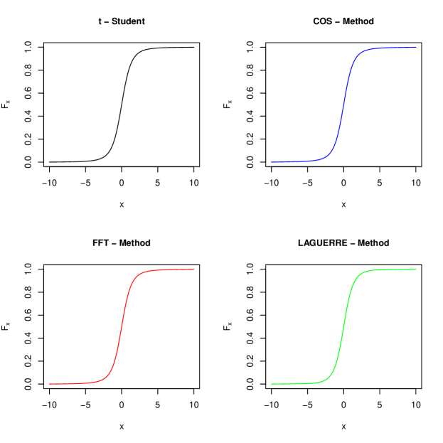
Figure 2. Cumulative distribution function comparison for a Student-$t$ random variable with $\nu=3$.

Figure 2 compares the cumulative distribution functions of the Student-$t$ obtained using the methods in YUIMA with the pt function. In all cases, we have a good level of precision that is also confirmed by Table 1. As expected the fastest method is the FFT which seems to be also the most precise.

	COS	FFT	LAG
RMSE	0.021	0.021	0.064
Max	0.032	0.032	0.085
Min	7.88e-05	2.18e-05	4.97e-04
sec.	1.47	4.00e-02	1.2

Table 1. Summary comparison of the distance between each method available in YUIMA and the cumulative distribution function obtained using the R function pt.

To further investigate this fact, we study the behaviour of the cumulative distribution function when $h$ varies. For $h=0.01$, we observe an oscillatory behaviour on tails for the FFT and COS while the Laguerre method seems to be more stable as shown in Figure 3. To have a fair comparison, we set N = 180, however we notice that the precision of FFT can be drastically improved by tuning the inputs N, up and low.

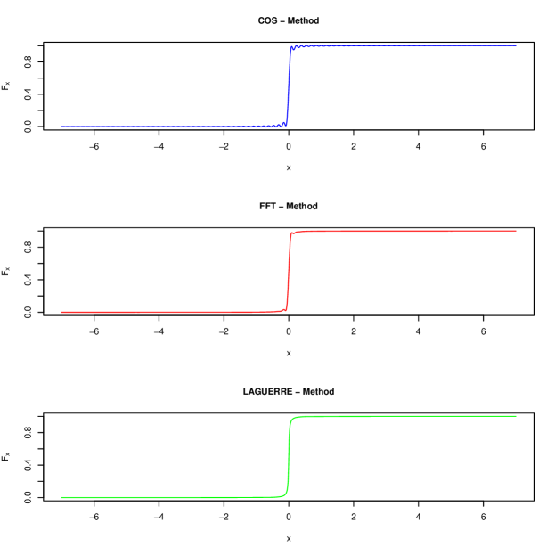
Figure 3. Cumulative distribution function comparison for a Student-$t$ Lévy increment with $\nu=3$ and $h=0.01$.

4.3. Numerical examples

This section presents a series of numerical examples demonstrating the practical application of newly developed classes and methods within the Student-$t$ Regression model. Specifically, we showcase the simulation and estimation of models where the regressors are determined by deterministic functions of time in the first example. The second example introduces integrated stochastic regressors. Lastly, we perform an analysis using real data in the final example.

4.3.1. Model with deterministic regressors.

In this example, we consider two deterministic regressors and the dynamics of the model have the following form:

(4.18) $$Y_{t}=\mu_{1}\cos\left(5t\right)+\mu_{2}\sin\left(t\right)+\sigma J_{t}$$

with the true values $\left(\mu_{1},\mu_{2},\sigma_{0},\nu_{0}\right)=\left(-5,-1,3,3\right)$. To use the simulation method in YUIMA we have to write the dynamics of the regressors $X_{1,t}:=\cos\left(5t\right)$ and $X_{2,t}=:\sin\left(5t\right)$, that is:

(4.19) $$\mbox{d}\left[\begin{array}[]{c}X_{1,t}\\ X_{2,t}\end{array}\right]=\left[\begin{array}[]{c}-5\sin\left(5t\right)\\ \cos\left(t\right)\end{array}\right]\mbox{d}t$$

with the initial condition:

$$X_{1,0}=1,\ X_{2,0}=0.$$

In the following, we show how to implement this model in YUIMA .

R> library(yuima)########### Inputs ############ Inputs for Fourier InversionR> method_Fourier = "FFT"; up = 6; low = -6; N = 2^17; N_grid = 60000# Inputs for the sample grid timeR> Factor <- 1R> Factor1 <- 1R> initial <- 0; Final_Time <- 50 * Factor; h <- 0.02/Factor1

We notice that the variable Factor1 controls the step size of the time grid. Indeed for different values of this quantity, we have a different value for $h$ for example Factor1 = 1, 2, 4, 7.2 corresponds h = 0.02, 0.01, 0.005, 1/365.

The first step is the definition of an object of yuima.th-class using the constructor setLaw_th. This object contains the random number generator, the density function, the cumulative distribution function and the quantile function for constructing the increments of a Student-$t$ Lévy process.

######################################## Example 1: Deterministic Regressors ########################################R> mu1 <- 5; mu2 <- -1; scale <- 3; nu <- 3 # Model Parameters# Model DefinitionR> law1 <- setLaw_th(method = method_Fourier, up = up, low = low,  N = N, N_grid = N_grid) # yuima.thR> class(yuima_law)

[1] "yuima.th"attr(,"package")[1] "yuima"

The next step is to define the dynamics of the regressors described in (4.19). This set of differential equations is defined in YUIMA using the standard constructor setModel. Once an object containing the mathematical description of the regressors has been defined, we use setLRM to obtain the yuima.LevyRM. In the following, we report the command lines for the definition of the Student Lévy Regression Model in (4.18).

R> regr1 <- setModel(drift = c("-5*sin(5*t)", "cos(t)"), diffusion = matrix("0",2,1),     solve.variable = c("X1","X2"), xinit = c(1,0)) # Regressors definitionR> Mod1 <- setLRM(unit_Levy = law1, yuima_regressors = regr1) # t-Regression ModelR> class(Mod1)

[1] "yuima.LevyRM"attr(,"package")[1] "yuima"

Using the object Mod1 we simulate a trajectory of the model in (4.18) using the YUIMA method simulate.

# SimulationR> samp <- setSampling(initial, Final_Time, n = Final_Time/h)R> true.par <- unlist(list(mu1 = mu1, mu2 = mu2, sigma0 = scale, nu = nu))R> set.seed(1)R> sim1 <- simulate(Mod1, true.parameter = true.par, sampling = samp) Figure 4 reports the simulated sample paths for the regressors $X_{1,t}$, $X_{2,t}$ and the Student Lévy Regression model $Y_{t}$.

Figure 4. Simulated Trajectory of the Student Lévy Regression model defined in (4.18).

The next step is to study the behaviour of the two-step estimation procedure described in Sections 2 and 3. To run this procedure, we use the method estimation_RLM and then we initialize randomly the optimization routine as shown in the following command lines.

# EstimationR> lower <- list(mu1 = -10, mu2 = -10,  sigma0 = 0.1)R> upper <- list(mu1 = 10, mu2 = 10, sigma0 = 10.01)R> start <- list(mu1 = runif(1, -10, 10), mu2 = runif(1, -10, 10),+    sigma0 = runif(1, 0.01, 4))R> Bn <- 15*FactorR> est1 <- estimation_RLM(start = start, model = sim1, data = sim1@data,+    upper = upper, lower = lower, PT = Bn)R> class(est1)

[1] "yuima.qmle"attr(,"package")[1] "yuima"

R> summary(est1)

Quasi-Maximum likelihood estimationCall:estimation_RLM(start = start, model = sim1, data = sim1@data,    upper = upper, lower = lower, PT = Bn)Coefficients:        Estimate Std. Errormu1     5.029555 0.03538355mu2    -1.128905 0.18026088sigma0  2.425147 0.12523404nu      2.735344 0.47457435-2 log L: 3236.535 73.3833

It is also possible to construct the dataset without the method simulate. This result can be achieved by constructing an object of yuima.th-class that represents the increment of the Student-$t$ Lévy process on the time interval with length $h$.

# Dataset construction without YUIMAR> time_t <- index(get.zoo.data(sim1@data)[[1]])R> X1 <- zoo(cos(5*time_t), order.by = time_t)R> X2 <- zoo(sin(time_t), order.by = time_t)R> law1_h <- setLaw_th(h = h, method = method_Fourier, up = up, low = low,     N = N, N_grid = N_grid)R> print(c(law1_h@h,law1@h))

[1] 0.02 1.00 The object law1_h refers to the Student-$t$ Lévy increment over an interval with length $0.02$ as it can be seen looking at the slot ...@h.

R> set.seed(1)R> names(nu)<- "nu"R> J_t <- zoo(cumsum(c(0,rand(law1_h, Final_Time/h,nu))), order.by = time_t)R> Y <- mu1 * X1 + mu2 * X2 + scale/sqrt(nu) * J_tR> data1_a <- merge(X1, X2, Y)

The estimation is performed by means of the method estimation_RLM as in the previous example.

R> est1_a <- estimation_RLM(start = start, model = Mod1, data = setData(data1_a),+    upper = upper, lower = lower, PT = Bn)R> summary(est1_a)

Quasi-Maximum likelihood estimationCall:estimation_RLM(start = start, model = Mod1, data = setData(data1_a),    upper = upper, lower = lower, PT = Bn)Coefficients:        Estimate Std. Errormu1     4.987778 0.03642823mu2    -1.164138 0.18558422sigma0  2.495930 0.12888927nu      2.407683 0.41221590-2 log L: 3232.784 85.32438

Based on the aforementioned examples, the estimated value for the $\sigma$ parameter deviates from its true value. To further investigate this observation, we conducted a comparative analysis using the three integration methods discussed in Section 4.2. This exercise was repeated for three different values of $h=0.01,0.005$ and $\frac{1}{365}$. To ensure a fair comparison among the Laguerre, Cosine Series expansion, and Fast Fourier Transform methods, we set the argument N = 180. The obtained results are presented in Table 2.

	Laguerre Method			COS Method			FFT Method
$h$	0.01	0.005	$1/365$	0.01	0.005	$1/365$	0.01	0.005	$1/365$
$\hat{\mu_{1}}$	4.968	5.019	4.976	4.939	5.065	4.875	4.934	5.069	4.876
	(0.029)	(0.020)	(0.014)	(0.041)	(0.049)	(0.054)	(0.042)	(0.049)	(0.054)
$\hat{\mu_{2}}$	-1.065	-1.044	-0.914	-1.192	-1.195	-0.555	-1.179	-1.178	-0.528
	(0.146)	(0.104)	(0.074)	(0.210)	(0.247)	(0.277)	(0.213)	(0.248)	(0.277)
$\hat{\sigma_{0}}$	2.770	2.794	2.657	3.993	6.654	10.010	4.055	6.674	10.010
	(0.101)	(0.072)	(0.051)	(0.145)	(0.172)	(0.192)	(0.148)	(0.172)	(0.193)
$\hat{\nu}$	3.462	3.281	3.067	2.827	2.223	2.227	5.749	8.310	15.175
	(0.615)	(0.580)	(0.538)	(0.492)	(0.377)	(0.378)	(1.063)	(1.571)	(2.940)
sec.	2.07	2.02	2.07	1.10	1.24	1.34	0.15	0.24	0.39

Table 2. Estimated parameters for $h=0.01,0.005,1/365$ and different integration methods. The number of points for the inversion of the characteristic function is $N=180$. The parenthesis shows the asymptotic standard error. The last row reports the seconds necessary for the simulation of a sample path.

In the Laguerre method, we observe that reducing the step size $h$ leads to improved estimates of $\nu$, however looking at the asymptotic standard error, the estimates for $\sigma_{0}$ seem to maintain the bias. As for the remaining methods, the estimates exhibit unsatisfactory performance due to the imposed restriction of N = 180 (that is the maximum value allowed for the Laguerre quadrature in R package statmod). This outcome is not unexpected, given the Laguerre method’s ability to yield a valid distribution even with a relatively small value of N, as demonstrated in Figure 3. Nevertheless for the COS and the FFT, it is possible to enhance the results by increasing the value of the argument N that yields a more accurate better result in the simulation of the sample path for the model described in (4.18).

	COS Method			FFT Method
N	1000	5000	10000	1000	5000	10000
$\mu_{1}$	4.968	4.975	4.975	4.968	4.975	4.975
	(0.034)	(0.016)	(0.016)	(0.035)	(0.306)	(0.016)
$\mu_{2}$	-0.887	-0.909	-0.909	-0.886	-0.908	-0.908
	(0.174)	(0.082)	(0.082)	(0.177)	(0.022)	(0.082)
$\sigma_{0}$	3.300	2.964	2.964	3.363	2.963	2.964
	(0.064)	(0.057)	(0.057)	(0.065)	(0.057)	(0.057)
$\nu$	2.713	2.765	2.765	3.279	2.760	2.702
	(0.470)	(0.480)	(0.480)	(0.579)	(0.479)	(0.468)
sec.	3.49	14.83	33.70	0.38	0.44	0.45

Table 3. Estimated parameters for $N=1000,5000,10^{4}$ in the COS and the FFT methods. The step size $h$ is $1/365$. The parenthesis shows the asymptotic standard error. The last row reports the seconds necessary for the simulation of a sample path.

Table 3 shows the estimated parameters for the varying value of N and $h=1/365$. As expected increasing the precision in the quadrature improved estimates for both methods. Notably for N $\geq$ 5000, all estimates fall within the asymptotic confidence interval at the $95\%$ level.

4.3.2. Model with integrated stochastic regressors

In this section, we consider two examples whose regressors are stochastic. Moreover, to satisfy Assumption 2.1, the regressors are supposed to be an integrated version of stochastic processes.

Example 1

In this example, we consider the following continuous time regression model with a single regressor:

$$Y_{t}=\mu\int_{0}^{t}X_{u}du+\sigma J_{t},\quad J_{1}\sim t_{\nu},$$

with the true values $(\mu_{0},\sigma_{0},\nu_{0})=(-3,3,2.5)$, and the process $X$ is supposed to be the Lévy driven Ornstein-Uhlenbeck process defined as:

$$dX_{t}=-X_{t}dt+2dZ_{t},$$

where the driving noise $Z$ is the Lévy process with $Z_{1}\sim\text{NIG}(1,0,1,0)$. The normal inverse Gaussian (NIG) random variable is defined as the normal-mean variance mixture of the inverse Gaussian random variable, and the probability density function of $Z_{t}\sim\text{NIG}(\alpha,\beta,\delta t,\mu t)$ is given by

$$x\mapsto\frac{\alpha\delta t\exp\{\delta t\sqrt{\alpha^{2}-\beta^{2}}+\beta(x-\mu t)\}K_{1}(\alpha\psi(x;\delta t,\mu t))}{\pi\psi(x;\delta t,\mu t)}$$

where $\alpha^{2}:=\gamma^{2}+\beta^{2}$ and $\psi(x;\delta t,\mu t):=\sqrt{(\delta t)^{2}+(x-\mu t)^{2}}$. More detailed theoretical properties of the NIG-Lévy process are given for example in [3].

For the simulation by YUIMA, we formally introduce the following system:

(4.20) $$d\Bigg{[}\begin{array}[]{c}X_{1,t}\\ X_{2,t}\end{array}\Bigg{]}=\Bigg{[}\begin{array}[]{c}X_{2,t}\\ -X_{2,t}\end{array}\Bigg{]}dt+\Bigg{[}\begin{array}[]{c}0\\ 2\end{array}\Bigg{]}dZ_{t},$$

with the initial condition:

$$X_{1,0}=0,\ X_{2,0}=0.$$

The process $X_{1,t}$ corresponds to the regressor in the regression model (4.3.2). Due to the specification of the new YUIMA function, we will additionally construct the “full” model:

$$Y_{t}=\mu_{1}X_{1,t}+\mu_{2}X_{2,t}+\sigma J_{t},\quad J_{1}\sim t_{\nu},$$

and simulate the trajectory of $Y$ with $\mu_{2}=0$. After that, we will estimate the parameters $(\mu_{1},\sigma,\nu)$ by the original model (4.3.2). From now on, we show the implementation of this model in YUIMA .

R> library(yuima)########### Inputs ############ Inputs for Fourier InversionR> method_Fourier = "FFT"; up = 6; low = -6; N = 2^17; N_grid = 60000# Inputs for the sample grid timeR> Factor <- 1R> Factor1 <- 1R> initial <- 0; Final_Time <- 50 * Factor; h <- 0.02/Factor1

The role of the variable Factor1 is the same as in the previous section. By using the constructor setLaw_th, we define yuima.th-class in a similar manner. After that we construct the “full” model (4.3.2) by the constructors setModel and setLRM. A trajectory of $Y$ and its regressors can be simulated by the YUIMA method simulate.

##################################################### Regressor: Integrated NIG-Levy driven OU process #####################################################R> mu1 <- -3; mu2 <- 0;  scale <- 3; nu <- 2.5 # Model Parameters# Model DefinitionR> lawILOU <- setLaw_th(method = method_Fourier, up = up, low = low, N = N,+    N_grid = N_grid) # yuima.thR> regrILOU <- setModel(drift = c("X2", "-X2"), jump.coeff = c("0", "2"),+    solve.variable = c("X1","X2"), xinit = c(0,0), measure.type = "code",+    measure = list(df = "rNIG(z, 1, 0, 1, 0)")) # Regressors definition# t-Regression modelR> ModILOU <- setLRM(unit_Levy = lawILOU, yuima_regressors = regrILOU)# SimulationR> sampILOU <- setSampling(initial, Final_Time, n = Final_Time/h)R> true.parILOU <- unlist(list(mu1 = mu1, mu2 = mu2, sigma0 = scale, nu = nu))R> set.seed(1)R> simILOU <- simulate(ModILOU, true.parameter = true.parILOU, sampling = sampILOU)

Next we extract the trajectories of $Y$ and $X_{1}$ from the yuima.LevyRM-class: simILOU and construct the new model for the estimation of the parameters. Figure 5 shows the simulated sample paths for the regressor and the Student Lévy Regression model $Y$.

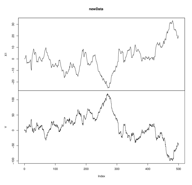
Figure 5. Simulated Trajectory of the Student Lévy Regression model defined in (4.3.2).

# Data extractionR> Dataset<-get.zoo.data(simILOU)R> newData <-Dataset[-2]R> newData <- merge(newData$X1, newData$Y)R> colnames(newData) <- c("X1","Y")R> plot(newData)# Define the model for estimationR> regrILOU1 <- setModel(drift = c("0"), diffusion = matrix(c("0"),1,1),+    solve.variable = c("X1"), xinit = c(0)) # Regressors definition# t-Regression modelR> ModILOU1 <- setLRM(unit_Levy = lawILOU, yuima_regressors = regrILOU1)# EstimationR> lower1 <- list(mu1 = -10,  sigma0 = 0.1)R> upper1 <- list(mu1 = 10, sigma0 = 10.01)R> startILOU1<- list(mu1 = runif(1, -10, 10), sigma0 = runif(1, 0.01, 4))R> Bn <- 15*FactorR> Data1 <- setData(newData)R> estILOU1 <- estimation_RLM(start = startILOU1, model = ModILOU1, data = Data1,+    upper = upper1, lower = lower1, PT = Bn)R> summary(estILOU1)

Quasi-Maximum likelihood estimationCall:estimation_RLM(start = startILOU1, model = ModILOU1, data = Data1,    upper = upper1, lower = lower1, PT = Bn)Coefficients:        Estimate Std. Errormu1    -2.959621 0.02112734sigma0  2.778659 0.03208519nu      2.404843 0.13018410-2 log L: 69711.32 854.3838

Example 2

In this example, we consider the following regression model:

$$Y_{t}=\mu_{1}\int_{0}^{t}V_{1,u}du+\mu_{2}\int_{0}^{t}V_{2,u}du+\sigma J_{t},\ \quad J_{1}\sim t_{\nu}$$

where the process $X=(V_{1},V_{2})$ satisfy

(4.21) $$dV_{1,t}=\frac{1}{\epsilon}(V_{1,t}-V_{1,t}^{3}-V_{2,t}+s)dt,$$

(4.22) $$dV_{2,t}=(\gamma V_{1,t}-V_{2,t}+\alpha)dt+\sigma^{\prime}dw_{t},$$

with

$$(\epsilon,s,\gamma,\alpha,\sigma^{\prime})=(1/3,0,3/2,1/2,2),$$

and standard Wiener process $w$. We set the true values

$$(\mu_{1,0},\mu_{2,0},\sigma_{0},\nu_{0})=(8,-4,8,3).$$

The process $V$ is the so-called stochastic FitzHugh-Nagumo process which is a classical model for describing a neuron; $V_{1}$ expresses the membrane potential of the neuron and $V_{2}$ represents a recovery variable. Its theoretical properties such as hypoellipticity, and Feller and mixing properties are well summarized in [18]. The paper also provides a nonparametric estimator of the invariant density and spike rate. Similarly, other integrated degenerate diffusion can be considered as regressors. Its ergodicity for our Assumption 2.1 is studied for example in [33]. For the statistical inference for degenerate diffusion processes, we refer to [9] and [12].

For the implementation of the regression model (4.3.2) on YUIMA, we formally consider the following dynamics:

(4.23) $$d\left[\begin{array}[]{c}X_{1,t}\\ X_{2,t}\\ X_{3,t}\\ X_{4,t}\end{array}\right]=\left[\begin{array}[]{c}X_{3,t}\\ X_{4,t}\\ 3(X_{3,t}-X_{3,t}^{3}-X_{4,t})\\ \frac{3}{2}X_{3,t}-X_{4,t}+\frac{1}{2}\end{array}\right]dt+\left[\begin{array}[]{c}0\\ 0\\ 0\\ 2\end{array}\right]dw_{t},$$

with the initial condition:

$$X_{1,0}=0,\ X_{2,0}=0,\ X_{3,0}=0,\ X_{4,0}=0.$$

The first and second elements correspond to the regressor in (4.3.2). As in the previous example, we first simulate data by the “full” model defined as:

(4.24) $$Y_{t}=\mu_{1}X_{1,t}+\mu_{2}X_{2,t}+\mu_{3}X_{3,t}+\mu_{4}X_{4,t}+\sigma J_{t},\quad J_{1}\sim t_{\nu},$$

with $\mu_{3}=\mu_{4}=0$, and after that, we extract the simulated data and estimate the parameters based on the original regression model (4.3.2). Below we show how to implement on YUIMA.

R> library(yuima)########### Inputs ############ Inputs for Fourier InversionR> method_Fourier = "FFT"; up = 6; low = -6; N = 2^17; N_grid = 60000# Inputs for the sample grid timeR> Factor <- 20R> Factor1 <- 4R> initial <- 0; Final_Time <- 50 * Factor; h <- 0.02/Factor1############################################################# Regressor: Integrated stochastic FitzHugh-Nagumo process #############################################################R> mu1 <- 8; mu2 <- -4; mu3 <- 0; mu4 <- 0;  scale <- 8; nu <- 3 # Model Parameters# Model DefinitionR> lawFN <- setLaw_th(method = method_Fourier, up = up, low = low,+    N = N, N_grid = N_grid) # yuima.thR> regrFN <- setModel(drift = c("X3", "X4", "3*(X3-X3^3-X4)", "1.5*X3-X4+0.5"),+    diffusion = matrix(c("0", "0", "0", "2"),4,1),+    solve.variable = c("X1","X2", "X3", "X4"),+    xinit = c(0,0,0,0)) # Regressors definitionR> ModFN <- setLRM(unit_Levy = lawFN, yuima_regressors = regrFN) #  t-regression model# SimulationR> sampFN <- setSampling(initial, Final_Time, n = Final_Time/h)R> true.parFN <- unlist(list(mu1 = mu1, mu2 = mu2, mu3 = mu3, mu4 = mu4,+    sigma0 = scale, nu = nu))R> set.seed(12)R> simFN <- simulate(ModFN, true.parameter = true.parFN, sampling = sampFN)

In this example, both Factor and Factor1 are larger than the previous example, and hence it takes a higher computational load than the previous one. Figure 6 shows the simulated sample paths for the regressor and the Student Lévy Regression model $Y$. Now we move on to the estimation phase.

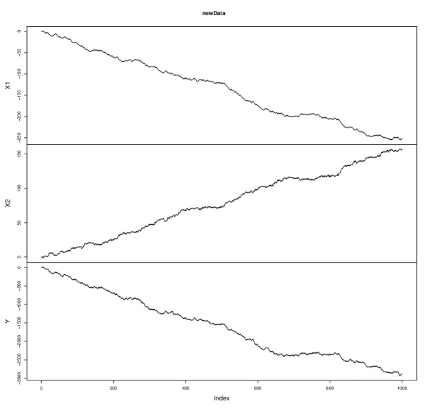
Figure 6. Simulated Trajectory of the Student Lévy Regression model defined in (4.3.2).

R> Dataset<-get.zoo.data(simFN)R> newData <-Dataset[-c(3,4)]R> newData <- merge(newData$X1,newData$X2, newData$Y)R> colnames(newData) <- c("X1","X2", "Y")R> plot(newData)# Define the model for estimationR> regrFN1 <- setModel(drift = c("0", "0"), diffusion = matrix(c("0", "0"),2,1),+    solve.variable = c("X1", "X2"), xinit = c(0,0)) # Regressors definitionR> ModFN1 <- setLRM(unit_Levy = lawFN, yuima_regressors = regrFN1) # t-Regression model.# EstimationR> lower1 <- list(mu1 = -10, mu2 = -10,  sigma0 = 0.1)R> upper1 <- list(mu1 = 10, mu2 =10, sigma0 = 10.01)R> startFN1<- list(mu1 = runif(1, -10, 10), mu2 = runif(1, -10, 10),+    sigma0 = runif(1, 0.01, 4))R> Bn <- 15*FactorR> Data1 <- setData(newData)R> estFN1 <- estimation_RLM(start = startFN1, model = ModFN1, data = Data1,+    upper = upper1, lower = lower1, PT = Bn)R> summary(estFN1)

Quasi-Maximum likelihood estimationCall:estimation_RLM(start = startFN1, model = ModFN1, data = Data1,    upper = upper1, lower = lower1, PT = Bn)Coefficients:        Estimate Std. Errormu1     8.041838 0.04895791mu2    -4.041518 0.04495255sigma0  7.712157 0.04452616nu      3.020972 0.11837331-2 log L: 403960.9 1291.516

4.4. Real data regressors

In this section, we show how to use the YUIMA package for the estimation of a Student Lévy Regression model in a real dataset. We consider a model where the daily price of the Standard and Poor 500 Index is explained by the VIX index and two currency rates: the YEN-USD and the Euro Usd rates. The dataset was provided by Yahoo.finance and ranges from December 14th 2014 to May 12th 2023. We downloaded the data using the function getSymbol available in quantmod library. To consider a small value for the step size $h$ we estimate our model every month (i.e.: $h=1/30$). We report below the code for storing the market data in an object of yuima.data-class

R> library(yuima)R> library(quantmod)R> getSymbols("^SPX", from = "2014-12-04", to = "2023-05-12")# RegressorsR> getSymbols("EURUSD=X", from = "2014-12-04", to = "2023-05-12")R> getSymbols("VIX", from = "2014-12-04", to = "2023-05-12")R> getSymbols("JPYUSD=X", from = "2014-12-04", to = "2023-05-12")R> SP <- zoo(x = SPX$SPX.Close, order.by = index(SPX$SPX.Close))R> Vix <- zoo(x = VIX$VIX.Close/1000, order.by = index(VIX$VIX.Close))R> EURUSD <- zoo(x = ‘EURUSD=X‘[,4], order.by = index(‘EURUSD=X‘))R> JPYUSD <- zoo(x = ‘JPYUSD=X‘[,4], order.by = index(‘JPYUSD=X‘))R> Data <- na.omit(na.approx(merge(Vix, EURUSD, JPYUSD, SP)))R> colnames(Data) <- c("VIX", "EURUSD", "JPYUSD", "SP")R> days <- as.numeric(index(Data))-as.numeric(index(Data))[1]# equally spaced grid time dataR> Data <- zoo(log(Data), order.by = days)R> Data_eq <- na.approx(Data, xout = days[1] : tail(days,1L))R> yData <- setData(zoo(Data_eq, order.by = index(Data_eq)/30)) # Data on monthly basis We decided to work with log-price (see Data variable in the above code) to have quantities defined on the same support of a Student-$t$ Lévy process, i.e.: the real line. Since the estimation method in YUIMA requires that the data are observed on an equally spaced grid time, we interpolate linearly to estimate possible missing data to get a log price for each day. Figure 7 shows the trajectory for each financial series.

Figure 7. Financial data observed on a monthly equally grid time ranging from December 14th 2014 to May 12th 2023.

To estimate the model we perform the same steps discussed in the previous examples and we report below the code for reproducing our result.

# Inputs for integration in the inversion formulaR> method_Fourier <- "FFT"; up <- 6; low <- -6; N <- 10000; N_grid <- 60000# Model DefinitionR> law <- setLaw_th(method = method_Fourier, up = up, low = low, N = N,+    N_grid = N_grid)R> regr <- setModel(drift = c("0", "0", "0"), diffusion = matrix("0",3,1),+    solve.variable = c("VIX", "EURUSD", "JPYUSD"), xinit = c(0,0,0))Mod <- setLRM(unit_Levy = law, yuima_regressors = regr, LevyRM = "SP")# EstimationR> lower <- list(mu1 = -100, mu2 = -200, mu3 = -100,  sigma0 = 0.01)R> upper <- list(mu1 = 100, mu2 = 100, mu3 = 100, sigma0 = 200.01)R> start <- list(mu1 = runif(1, -100, 100), mu2 = runif(1, -100, 100),+    mu3 = runif(1, -100, 100), sigma0 = runif(1, 0.01, 100))R> est <- estimation_RLM(start = start, model = Mod, data = yData, upper = upper,+    lower = lower, PT = floor(tail(index(Data_eq)/30,1L)/2))R> summary(est)

Quasi-Maximum likelihood estimationCall:estimation_RLM(start = start, model = Mod, data = yData, upper = upper,    lower = lower, PT = floor(tail(index(Data_eq)/30, 1L)/2))Coefficients:           Estimate  Std. Errormu1     0.000335328 0.004901559mu2    -0.062235188 0.033027232mu3     0.016291220 0.039382559sigma0  0.082031691 0.004859138nu      3.062728822 0.616466913-2 log L: -1506.067 48.17592

4.5. Analysis of estimator behavior in simulation exercises

In this section, we analyze the behavior of estimators for regressor parameters, scale coefficient, and degree of freedom through two simulation exercises within the context of a Student Lévy Regression model. The objective is to evaluate the performance of the studentized estimators using the simulated distributions and assess the suitability of standard normal approximations.

For the first simulation exercise, we set $T_{n}=400$, $B_{n}=20$ and $h=\frac{1}{200}$. We simulate 1000 trajectories of the model with deterministic regressors in (4.18) with $\mu_{1}=5$, $\mu_{2}=-1$, $\sigma_{0}=3$ and $\nu=1$. Estimating the parameters for each trajectory, we obtain the empirical distribution of the studentized estimates. To strike a balance between computational time and numerical inversion precision, we adopt the following values: up = 100, low = 100, N = 2${}^{\texttt{16}}$ and N_grid = 10${}^{\texttt{5}}$. Figure 8 shows the simulated distribution of studentized estimates. Notably, all histograms demonstrate that the standard normal approximation adequately captures the behavior of model parameters. Favorable results are obtained for the regressors $\left(\mu_{1},\mu_{2}\right)$ and the scale coefficient $\sigma_{0}$. However, a small upward bias appears for the degree of freedom $\nu$. This bias can be controlled by increasing the numerical precision and/or considering a larger value for $T_{n}$.

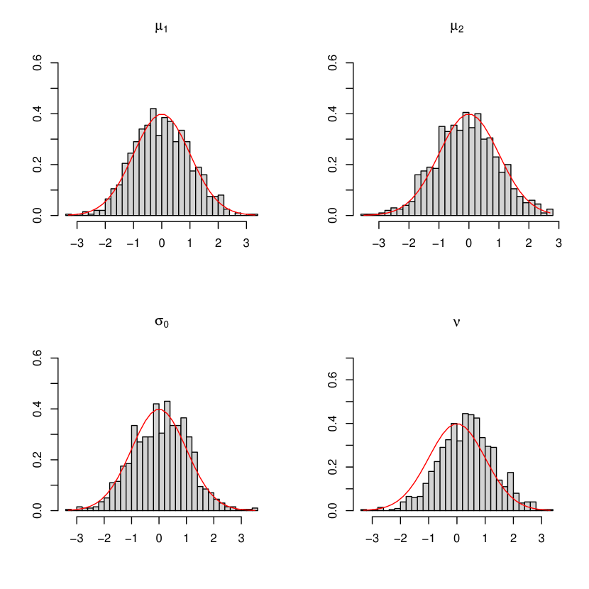
Figure 8. Simulated distribution of studentized parameters. In this case, we have $\mu_{1}=5$, $\mu_{2}=-1$, $\sigma_{0}=3$ and $\nu=1$.

In the second simulation exercise, we focus on the case of $\nu=2$. To achieve a good normal approximation, we adjust the step size to $h=\frac{1}{300}$ and reduce the numerical precision (up = 30, low = 30) to maintain consistent simulation time (approximately 1h) compared to the previous study. All other inputs remain unchanged. The comparison demonstrates a favorable agreement between the simulated density functions and the standard normal distribution for all model parameters. This comparison suggests that a larger value of the degree of freedom $\nu$ requires a smaller step-size value $h$ to ensure accurate approximations.

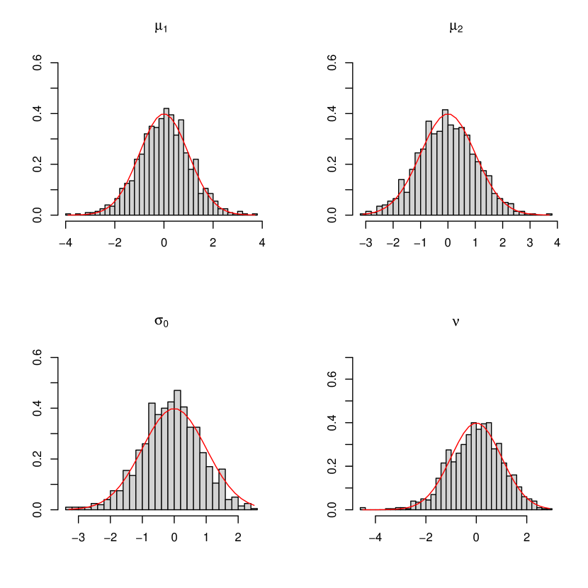
Figure 9. Simulated distribution of studentized parameters. In this case, we have $\mu_{1}=5$, $\mu_{2}=-1$, $\sigma_{0}=3$ and $\nu=2$.

In conclusion, the analysis of estimator behavior through these simulation exercises provides valuable insights into their performance within the Student Lévy Regression model. The results indicate satisfactory performance for most estimators, with minor biases observed for the degree of freedom parameter. Adjustments in numerical precision and step-time interval can effectively control these biases.

5. Proofs

5.1. Proof of Theorem 2.2

Let

$$\mathbb{Y}_{1,n}(a) :=\frac{1}{N_{n}}\left(\mathbb{H}_{1,n}(a)-\mathbb{H}_{1,n}(a_{0})\right),$$

$$\Gamma_{a,n} :=-\frac{1}{N_{n}}\partial_{a}^{2}\mathbb{H}_{1,n}(a_{0}).$$

We will prove the following three lemmas.

Lemma 5.1.

Under (2.2) and Assumption 2.1, there exist a non-random function $\mathbb{Y}_{1}:\,\overline{\Theta_{\mu}\times\Theta_{\sigma}}\to\mathbb{R}$ and constants $c_{0}>0$ and $c_{2}\in(0,1/2]$ such that for all $K>0$,

(5.1) $$\sup_{n}E\left[\sup_{a}\big{(}N_{n}^{c_{2}}\left|\mathbb{Y}_{1,n}(a)-\mathbb{Y}_{1}(a)\right|\big{)}^{K}\right]<\infty,$$

and that for all $a\in\Theta_{\mu}\times\Theta_{\sigma}$,

(5.2) $$\mathbb{Y}_{1}(a)\leq-c_{0}|a-a_{0}|^{2}.$$

Lemma 5.2.

Under (2.2) and Assumption 2.1, there exist a constant $c_{1}\in(0,1/2)$ such that for every $K>0$,

(5.3) $$\sup_{n}E\left[|\Delta_{a,n}|^{K}\right]+\sup_{n}E\left[\left(N_{n}^{c_{1}}\left|\Gamma_{a,n}-\Gamma_{a,0}\right|\right)^{K}\right]+\sup_{n}E\left[\sup_{a}\left|\frac{1}{N_{n}}\partial_{a}^{3}\mathbb{H}_{1,n}(a)\right|^{K}\right]<\infty.$$

Lemma 5.3.

Under (2.2) and Assumption 2.1, we have $\left(\Delta_{a,n},\,\Gamma_{a,n}\right)\xrightarrow{\mathcal{L}}\big{(}\Gamma_{a,0}^{1/2}\eta,\,\Gamma_{a,0}\big{)}$, where $\eta\sim N_{q+1}(0,I_{q+1})$.

Theorem 2.2 follows from these lemmas: with Lemmas 5.1 and 5.2, we can establish the tail-probability estimate (2.10) through [34, Theorem 3(c)]; moreover, the asymptotic normality (2.9) follows from the standard likelihood-asymptotics argument together with Lemmas 5.3. We omit the details.

By (1.4), the probability density of $\mathcal{L}(h^{-1}J_{h})$ is given by

$$f_{h}(y;\nu) =\frac{1}{2\pi}\int\cos(uy)\left\{\varphi_{J_{1},\nu}(h^{-1}u)\right\}^{h}du$$

(5.4) $$=\left(\frac{2^{1-\nu/2}h^{-\nu/2}}{\Gamma(\nu/2)}\right)^{h}\frac{h}{\pi}\int_{0}^{\infty}\cos(uhx)u^{\nu h/2}\left(K_{\nu/2}(u)\right)^{h}du,$$

the existence of which is ensured by [4, Proposition 1] together with the locally Cauchy property $h^{-1}J_{h}\xrightarrow{\mathcal{L}}t_{1}$. The next lemma quantifies the speed of the local Cauchy approximation in $L^{1}(dy)$ and serves as a basic tool for deriving limit theorems.

Lemma 5.4.

For any $r>0$ and any measurable function $\zeta:\mathbb{R}\to\mathbb{R}$ such that $|\zeta(y)|\lesssim 1+\{\log(1+|y|)\}^{K}$ for some $K>0$, we have

(5.5) $$\int\left|\zeta(y)\right|\left|f_{h}(y)-\phi_{1}(y)\right|dy\lesssim h^{1-r}.$$

In particular, under (2.2) we have

(5.6) $$\sqrt{N_{n}}\int\left|\zeta(y)\right|\left|f_{h}(y)-\phi_{1}(y)\right|dy\to 0.$$

Related remarks on the estimate under the total variation distance can be found in [7, Remark 2.1].

5.1.1. Proof of Lemma 5.1

Let $\epsilon_{j}:=\epsilon_{j}(a_{0})$; then, $\epsilon_{1},\epsilon_{2}\dots\sim\text{i.i.d.}~{}\mathcal{L}(h^{-1}J_{h})$, which admits the density $f_{h}(y)$ defined by (5.4). We have

$$\epsilon_{j}(a) =\frac{\sigma_{0}}{\sigma}\epsilon_{j}-\frac{1}{\sigma}(\mu-\mu_{0})\cdot X^{\prime}_{t_{j-1}}-\frac{1}{\sigma}(\mu-\mu_{0})\cdot R_{n,j},$$

where $R_{n,j}:=h^{-1}(\Delta_{j}X-hX^{\prime}_{t_{j-1}})$. Let $g_{1}(\epsilon):=\partial_{\epsilon}\phi_{1}(\epsilon)/\phi_{1}(\epsilon)$ and

(5.7) $$\zeta(y,X^{\prime}_{t_{j-1}};\,a):=\log\left[\frac{\sigma_{0}}{\sigma}\phi_{1}\left(\frac{\sigma_{0}}{\sigma}\left(y-\frac{1}{\sigma_{0}}(\mu-\mu_{0})\cdot X^{\prime}_{t_{j-1}}\right)\right)\right]-\log\phi_{1}(y).$$

Then, we have the decomposition $\mathbb{Y}_{1,n}(a)=\mathbb{Y}_{1,n}^{\ast}(a)+\delta_{11,n}(a)$ where

(5.8) $$\mathbb{Y}_{1,n}^{\ast}(a) =\frac{1}{N_{n}}\sum_{j=1}^{N_{n}}\zeta(\epsilon_{j},X^{\prime}_{t_{j-1}};\,a),$$

$$\delta_{11,n}(a) :=-\frac{1}{N_{n}}\sum_{j=1}^{N_{n}}\int_{0}^{1}g_{1}\left(\frac{\sigma_{0}}{\sigma}\epsilon_{j}-\frac{1}{\sigma}(\mu-\mu_{0})\cdot X^{\prime}_{t_{j-1}}-\frac{s}{\sigma}(\mu-\mu_{0})\cdot R_{n,j}\right)ds$$

(5.9) $${}\qquad\times\frac{1}{\sigma}(\mu-\mu_{0})\cdot R_{n,j}.$$

By Assumption 2.1 and (2.2), we can pick a sufficiently small $c_{2}\in(0,\frac{c_{X}}{2-\epsilon^{\prime}}\wedge\frac{1}{2}]$ to obtain

$$\max_{j\leq N_{n}}E[|N_{n}^{c_{2}}R_{n,j}|^{K}]\lesssim\max_{j\leq N_{n}}E[|n^{c_{2}(2-\epsilon^{\prime})}R_{n,j}|^{K}]\leq\max_{j\leq[nT_{n}]}E[|n^{c_{2}(2-\epsilon^{\prime})}R_{n,j}|^{K}]\to 0.$$

Since $\|g_{1}\|_{\infty}<\infty$, for any $K>0$ we have

$$E\left[\sup_{a}|N_{n}^{c_{2}}\delta_{11,n}(a)|^{K}\right]\lesssim\max_{j\leq N_{n}}E[|N_{n}^{c_{2}}R_{n,j}|^{K}]\to 0.$$

Write $E^{j-1}[\cdot]=E[\cdot|\mathcal{F}_{t_{j-1}}]$. Then,

(5.10) $$\mathbb{Y}_{1,n}^{\ast}(a) =:\frac{1}{N_{n}}\sum_{j=1}^{N_{n}}\chi_{j}(a)$$

$$=\frac{1}{\sqrt{N_{n}}}\sum_{j=1}^{N_{n}}\frac{1}{\sqrt{N_{n}}}\widetilde{\chi}_{j}(a)+\frac{1}{N_{n}}\sum_{j=1}^{N_{n}}E^{j-1}[\chi_{j}(a)],$$

where $\widetilde{\chi}_{j}(a)=\chi_{j}(a)-E^{j-1}[\chi_{j}(a)]$. Obviously,

$$\sup_{n}\sup_{a}\left(E\left[\left|\sum_{j=1}^{N_{n}}\frac{1}{\sqrt{N_{n}}}\widetilde{\chi}_{j}(a)\right|^{K}\right]+E\left[\left|\sum_{j=1}^{N_{n}}\frac{1}{\sqrt{N_{n}}}\partial_{a}\widetilde{\chi}_{j}(a)\right|^{K}\right]\right)<\infty$$

for any $K>2$. We are assuming that $\Theta$ is a bounded convex domain, hence can apply the Sobolev inequality [2, Theorem 1.4.2] to conclude that

(5.11) $$\sup_{n}E\left[\sup_{a}\left|\sum_{j=1}^{N_{n}}\frac{1}{\sqrt{N_{n}}}\widetilde{\chi}_{j}(a)\right|^{K}\right]<\infty.$$

This leads to

$$\sup_{n}E\left[\sup_{a}\left(N_{n}^{c_{2}}\left|\mathbb{Y}_{1,n}(a)-\frac{1}{N_{n}}\sum_{j=1}^{N_{n}}E^{j-1}[\chi_{j}(a)]\right|\right)^{K}\right]<\infty.$$

Observe that

$$\frac{1}{N_{n}}\sum_{j=1}^{N_{n}}E^{j-1}[\chi_{j}(a)]$$

$$=\frac{1}{N_{n}}\sum_{j=1}^{N_{n}}\int\zeta(y,X^{\prime}_{t_{j-1}};a)\phi_{1}(y)dy+\frac{1}{N_{n}}\sum_{j=1}^{N_{n}}\int\zeta(y,X^{\prime}_{t_{j-1}};a)(f_{h}(y)-\phi_{1}(y))dy$$

(5.12) $$=:\mathbb{Y}^{\ast\ast}_{1,n}(a)+\delta_{12,n}(a).$$

Note that $\sup_{a}|\zeta(y,X^{\prime}_{t_{j-1}};a)|\lesssim 1+\log(1+|X^{\prime}_{t_{j-1}}|)+\log(1+|y|)\lesssim\{1+\log(1+|X^{\prime}_{t_{j-1}}|)\}\{1+\log(1+|y|)\}$. Also, $N_{n}^{c_{2}}h^{1-c}\lesssim n^{c_{2}(2-\epsilon^{\prime})}n^{c-1}\to 0$ with $c_{2},c>0$ small enough. It follows from Lemma 5.4 and Assumption 2.1 that

$$E\left[\sup_{a}|N_{n}^{c_{2}}\delta_{12,n}(a)|^{K}\right] \lesssim\max_{j\leq N_{n}}E\left[\left|(1+|X^{\prime}_{t_{j-1}}|)^{C}N_{n}^{c_{2}}h^{1-c}\right|^{K}\right]$$

$$\lesssim(N_{n}^{c_{2}}h^{1-c})^{K}\sup_{0\leq t\leq hN_{n}}E\left[(1+|X^{\prime}_{t_{j-1}}|)^{C}\right]\to 0.$$

Now, we define

$$\mathbb{Y}_{1}(a):=\int\int\zeta(y,x^{\prime};a)\phi_{1}(y)dy\,\pi_{0}(dx^{\prime}).$$

By the definition (5.7) and the well-known property of the Kullback-Leibler divergence, we have $\mathbb{Y}_{1}(a)\leq 0$ with the equality holding if and only if $a=a_{0}$. Moreover, $\partial_{a}\mathbb{Y}_{1}(a_{0})=0$ holds and $-\partial_{a}^{2}\mathbb{Y}_{1}(a_{0})$ is positive definite. These observations conclude (5.2).

By piecing together what we have seen,

$$\sup_{n}E\left[\sup_{a}\big{(}N_{n}^{c_{2}}\left|\mathbb{Y}_{1,n}(a)-\mathbb{Y}_{1}(a)\right|\big{)}^{K}\right]$$

$$\lesssim 1+\sup_{n}E\left[\sup_{a}\big{(}N_{n}^{c_{2}}\left|\mathbb{Y}^{\ast\ast}_{1,n}(a)-\mathbb{Y}_{1}(a)\right|\big{)}^{K}\right]$$

$$\lesssim 1+\sup_{n}E\left[\sup_{a}\left(N_{n}^{c_{2}}\left|\frac{1}{hN_{n}}\int_{0}^{hN_{n}}\int\zeta(y,X^{\prime}_{t};a)\phi_{1}(y)dydt-\mathbb{Y}_{1}(a)\right|\right)^{K}\right]$$

$${}\qquad+\sup_{n}E\bigg{[}\sup_{a}\bigg{(}N_{n}^{c_{2}}\bigg{|}\frac{1}{N_{n}}\sum_{j=1}^{N_{n}}\int\zeta(y,X^{\prime}_{t_{j-1}};a)\phi_{1}(y)dy$$

(5.13) $${}\qquad\qquad\qquad-\frac{1}{hN_{n}}\int_{0}^{hN_{n}}\int\zeta(y,x^{\prime};a)\phi_{1}(y)dydt\bigg{|}\bigg{)}^{K}\bigg{]}.$$

We may and do set $c_{2}\in(0,\frac{\epsilon^{\prime\prime}}{2-\epsilon^{\prime}}c^{\prime}_{X}\wedge\frac{1}{2-\epsilon^{\prime}}c_{X}]\subset(0,c_{X}^{\prime}\wedge c_{X}]$. By (2.2), $N_{n}^{c_{2}}(hN_{n})^{-c^{\prime}_{X}}\lesssim n^{(2-\epsilon^{\prime})c_{2}-\epsilon^{\prime\prime}c_{X}^{\prime}}\lesssim 1$.

Let $f(x^{\prime},a):=\int\zeta(y,x^{\prime};a)\phi_{1}(y)dy$. Then, $\sup_{a}\{|f(x,a)|\vee|\partial_{a}f(x,a)|\}\lesssim 1+|x|^{C}$ (for any $C>0$) and $\mathbb{Y}_{1}(a)=\int f(x^{\prime},a)\pi_{0}(dx^{\prime})$. We decompose as follows:

$$\frac{1}{hN_{n}}\int_{0}^{hN_{n}}f(X^{\prime}_{t},a)dt-\int f(x^{\prime},a)\pi_{0}(dx^{\prime})$$

$$=\frac{1}{N_{n}}\sum_{j=1}^{N_{n}}\frac{1}{h}\int_{(j-1)/n}^{j/n}\big{(}f(X^{\prime}_{t},a)-f(X^{\prime}_{t_{j-1}},a)\big{)}dt$$

(5.14) $${}\qquad+\left(\frac{1}{N_{n}}\sum_{j=1}^{N_{n}}f(X^{\prime}_{t_{j-1}},a)-\int f(x^{\prime},a)\pi_{0}(dx^{\prime})\right)=:U_{1,n}(a)+U_{2,n}(a).$$

Apply the Jensen and Hölder inequalities to conclude that the first expectation in (5.13) is finite: for $1/p^{\prime}+1/q^{\prime}=1$,

$$E\left[\sup_{a}\big{|}N_{n}^{c_{2}}U_{1,n}(a)\big{|}^{K}\right]$$

$$\lesssim\frac{1}{N_{n}}\sum_{j=1}^{N_{n}}\frac{1}{h}\int_{(j-1)/n}^{j/n}E\left[(1+|X^{\prime}_{t}|^{C}+|X^{\prime}_{t_{j-1}}|^{C})\big{(}N_{n}^{c_{2}}|X^{\prime}_{t}-X^{\prime}_{t_{j-1}}|\big{)}^{K}\right]dt$$

$$\lesssim\frac{1}{N_{n}}\sum_{j=1}^{N_{n}}\frac{1}{h}\int_{t_{j-1}}^{t_{j}}\sup_{t}E[1+|X^{\prime}_{t}|^{C}]^{1/p^{\prime}}E\left[|N_{n}^{c_{2}}(X^{\prime}_{t}-X^{\prime}_{t_{j-1}})|^{Kq^{\prime}}\right]^{1/q^{\prime}}dt$$

$$\lesssim\max_{j=1,\dots,[nT_{n}]}\sup_{t_{j-1}\leq t\leq t_{j}}E\left[|N_{n}^{c_{2}}(X^{\prime}_{t}-X^{\prime}_{t_{j-1}})|^{Kq^{\prime}}\right]^{1/q^{\prime}}$$

(5.15) $$\lesssim\max_{j=1,\dots,[nT_{n}]}\sup_{t_{j-1}\leq t\leq t_{j}}E\left[|h^{-c_{X}}(X^{\prime}_{t}-X^{\prime}_{t_{j-1}})|^{Kq^{\prime}}\right]^{1/q^{\prime}}\lesssim 1.$$

Assumption 2.1(3) guarantees $\sup_{n}E[\sup_{a}|N_{n}^{c_{2}}U_{2,n}(a)|^{K}]<\infty$. The second expectation in (5.13) can be handled as in (5.15), followed by $\sup_{n}E[\sup_{a}(N_{n}^{c_{2}}|\mathbb{Y}_{1,n}(a)-\mathbb{Y}_{1}(a)|)^{K}]<\infty$.

5.1.2. Proof of Lemma 5.2

We will look at the three terms in (5.3) separately.

Quasi-score function

Write $\epsilon_{j}=\epsilon_{j}(a_{0})\sim\text{i.i.d.}~{}\mathcal{L}(h^{-1}J_{h})$. Direct calculations give

$$\Delta_{a,n} =-\sigma_{0}^{-1}\frac{1}{\sqrt{N_{n}}}\sum_{j=1}^{N_{n}}\begin{pmatrix}(h^{-1}\Delta_{j}X)g_{1}(\epsilon_{j})\\ 1+\epsilon_{j}g_{1}(\epsilon_{j})\end{pmatrix}$$

(5.16) $$=-\sigma_{0}^{-1}\frac{1}{\sqrt{N_{n}}}\sum_{j=1}^{N_{n}}\begin{pmatrix}X^{\prime}_{t_{j-1}}g_{1}(\epsilon_{j})\\ 1+\epsilon_{j}g_{1}(\epsilon_{j})\end{pmatrix}-\sigma_{0}^{-1}\frac{1}{N_{n}}\sum_{j=1}^{N_{n}}\begin{pmatrix}\sqrt{N_{n}}R_{n,j}\,g_{1}(\epsilon_{j})\\ 0\end{pmatrix}.$$

The first term in (5.16) equals

$$-\sigma_{0}^{-1}\frac{1}{\sqrt{N_{n}}}\sum_{j=1}^{N_{n}}\begin{pmatrix}X^{\prime}_{t_{j-1}}(g_{1}(\epsilon_{j})-E[g_{1}(\epsilon_{j})])\\ 1+\epsilon_{j}g_{1}(\epsilon_{j})-E[1+\epsilon_{j}g_{1}(\epsilon_{j})]\end{pmatrix}$$

$${}\qquad+\sigma_{0}^{-1}\frac{1}{N_{n}}\sum_{j=1}^{N_{n}}\sqrt{N_{n}}\begin{pmatrix}X^{\prime}_{t_{j-1}}(E[g_{1}(\epsilon_{j})]-\int g_{1}(y)\phi_{1}(y)dy)\\ E[1+\epsilon_{j}g_{1}(\epsilon_{j})]-\int(1+y\partial g_{1}(y))\phi_{1}(y)dy\end{pmatrix}.$$

(5.17) $$=:r^{\prime}_{1,n}+r^{\prime\prime}_{1,n}.$$

The Burkholder inequality gives the $L^{K}(P)$-boundedness of $(r^{\prime}_{1,n})_{n}$ for any $K>0$. By Lemma 5.4, the summand in $r^{\prime\prime}_{1,n}$ can be bounded in absolute value by a constant multiple of $(1+|X^{\prime}_{t_{j-1}}|)\sqrt{N_{n}}h^{1-c}\lesssim(1+|X^{\prime}_{t_{j-1}}|)n^{c-\epsilon^{\prime}/2}$. The sequence $(r^{\prime\prime}_{1,n})_{n}$ is also $L^{K}(P)$-bounded since $c>0$ can be taken arbitrarily small so that $c\leq\epsilon^{\prime}/2$.

For the second term in (5.16), by the compensation and the Burkholder inequality it suffices to show that for any $K\geq 2$,

$$\frac{1}{N_{n}}\sum_{j=1}^{N_{n}}E\left[\left|\sqrt{N_{n}}E^{j-1}[R_{n,j}\,g_{1}(\epsilon_{j})]\right|^{K}\right]=O(1).$$

This is ensured by Assumption 2.1.

Quasi-observed information

The components of $\Gamma_{a,n}$ consists of

$$-\frac{1}{N_{n}}\partial_{\mu}^{2}\mathbb{H}_{1,n}(a_{0}) =-\sigma_{0}^{-2}\frac{1}{N_{n}}\sum_{j=1}^{N_{n}}(h^{-1}\Delta_{j}X)^{\otimes 2}\partial g_{1}(\epsilon_{j}),$$

$$-\frac{1}{N_{n}}\partial_{\sigma}^{2}\mathbb{H}_{1,n}(a_{0}) =-\sigma_{0}^{-2}\frac{1}{N_{n}}\sum_{j=1}^{N_{n}}\left(1+2\epsilon_{j}g_{1}(\epsilon_{j})+\epsilon_{j}^{2}\partial g_{1}(\epsilon_{j})\right),$$

$$-\frac{1}{N_{n}}\partial_{\mu}\partial_{\sigma}\mathbb{H}_{1,n}(a_{0}) =-\sigma_{0}^{-2}\frac{1}{N_{n}}\sum_{j=1}^{N_{n}}(h^{-1}\Delta_{j}X)\left(g_{1}(\epsilon_{j})-\epsilon_{j}\partial g_{1}(\epsilon_{j})\right).$$

To conclude that $\sup_{n}E[(N_{n}^{c_{1}}|\Gamma_{a,n}-\Gamma_{a,0}|)^{K}]<\infty$, we note the following three preliminary steps (we can take $c_{1}>0$ as small as we want):

• First, we replace $h^{-1}\Delta_{j}X$ in the summands by $R_{n,j}+X^{\prime}_{t_{j-1}}$; this together with Assumption 2.1 enables us to replace $h^{-1}\Delta_{j}X$ in the summands by $X^{\prime}_{t_{j-1}}$;

• Second, we extract the martingale terms by replacing the parts of the form $\eta(\epsilon_{j})$ by $\eta(\epsilon_{j})-E[\eta(\epsilon_{j})]$ and then apply the Burkholder inequality to the latter parts;

• Third, we apply Lemma 5.4 with the facts $-\int\partial g_{1}(y)\phi_{1}(y)dy=1/2$, $-\int(1+2yg_{1}(y)+y^{2}\partial g_{1}(y))\phi_{1}(y)dy=1/2$, and $\int(g_{1}(y)-y\partial g_{1}(y))\phi_{1}(y)dy=0$.

Then, it remains to show that

$$\sup_{n}E\left[\left(N_{n}^{c_{1}}\left|\frac{1}{N_{n}}\sum_{j=1}^{N_{n}}X_{t_{j-1}}^{\prime\,\otimes 2}-S_{0}\right|\right)^{K}\right]<\infty.$$

This can be deduced similarly to the last paragraph in the proof of Lemma 5.1, hence omitted.

Third-order derivatives

We have

$$\frac{1}{N_{n}}\sup_{a}|\partial_{a}^{3}\mathbb{H}_{1,n}(a)|\lesssim\frac{1}{N_{n}}\sum_{j=1}^{N_{n}}\left(1+|h^{-1}\Delta_{j}X|\right),$$

hence $\sup_{n}E[\sup_{a}|N_{n}^{-1}\partial_{a}^{3}\mathbb{H}_{1,n}(a)|^{K}]<\infty$.

5.1.3. Proof of Lemma 5.3

We have $\Delta_{a,n}=r^{\prime}_{1,n}+o_{p}(1)$ from the arguments in Section 5.2 (with $c<\epsilon^{\prime}/2$). Write $r^{\prime}_{1,n}=\sum_{j=1}^{N_{n}}\zeta_{n,j}$. Then, the $(\mathcal{F}_{t_{j}})$-martingale difference array $(\zeta_{n,j})_{j\leq[nT_{n}]}$ satisfies the Lyapunov condition ($\sum_{j=1}^{N_{n}}E^{j-1}[|\zeta_{n,j}|^{\delta+2}]=o_{p}(1)$ for $\delta>0$). Also, by using Lemma 5.4 as in Section 5.2 together with the facts $\int g_{1}(y)^{2}\phi_{1}(y)dy=\int(1+yg_{1}(y))^{2}\phi_{1}(y)dy=1/2$ and $\int g_{1}(y)(1+yg_{1}(y))\phi_{1}(y)dy=0$, we obtain

$$\frac{1}{N_{n}}\sum_{j=1}^{N_{n}}E^{j-1}\left[\zeta_{n,j}^{\otimes 2}\right]$$

$$=\sigma_{0}^{-2}\frac{1}{N_{n}}\sum_{j=1}^{N_{n}}\begin{pmatrix}(h^{-1}\Delta_{j}X)^{\otimes 2}g_{1}(\epsilon_{j})^{2}&\text{sym.}\\ (h^{-1}\Delta_{j}X)g_{1}(\epsilon_{j})(1+\epsilon_{j}g_{1}(\epsilon_{j}))&(1+\epsilon_{j}g_{1}(\epsilon_{j}))^{2}\end{pmatrix}+o_{p}(1)$$

$$=\sigma_{0}^{-2}\frac{1}{N_{n}}\sum_{j=1}^{N_{n}}\begin{pmatrix}X^{\prime\otimes 2}_{t_{j-1}}\int g_{1}(y)^{2}\phi_{1}(y)dy&0\\ 0&\int(1+yg_{1}(y))^{2}\phi_{1}(y)dy\end{pmatrix}+o_{p}(1)$$

$$=\Gamma_{a,0}+o_{p}(1).$$

It follows that $\Delta_{a,n}\xrightarrow{\mathcal{L}}N_{q+1}(0,\Gamma_{a,0})$ by the central limit theorem for martingale difference arrays [31, Chapter VII.8]. The convergence $\Gamma_{a,n}\xrightarrow{p}\Gamma_{a,0}$ is automatic by the argument in Section 5.2; indeed, it holds almost surely by Borel-Cantelli lemma.

5.1.4. Proof of Lemma 5.4

As in [24, Example 2.7], our proof is based on the explicit form of the characteristic function (1.3). We will proceed similarly to the proof of [24, Lemma 2.2], with omitting some details of the calculation.

Let $g(z)$ denote the Lévy density of $\mathcal{L}(J_{1})$ and write $g(z)=\pi^{-1}|z|^{-2}(1+\rho(z))$. Then, by [29, Proposition 2.18] we have

(5.18) $$\rho(z)=\frac{\pi}{4}(1-\nu_{0})|z|+o(|z|),\qquad|z|\to 0.$$

Let $g_{0}(z):=(\pi y)^{-2}$, the Lévy density of $t_{1}$, and let $\varphi_{h}(u)$ and $\varphi_{0}(u)$ denote the characteristic functions of $\mathcal{L}(h^{-1}J_{h})$ and $t_{1}$, respectively; we have $\varphi_{0}(u)=\exp\{\int(\cos(uy)-1)g_{0}(y)dy\}=e^{-|u|}$ and already noted in (2.1) that

$$\varphi_{h}(u)=\left(\frac{2^{1-\nu/2}}{\Gamma(\nu/2)}\right)^{h}\left(|u/h|^{\nu/2}K_{\nu/2}(|u/h|)\right)^{h}\to\varphi_{0}(u),\quad h\to 0.$$

By straightforward computations, we obtain $\varphi_{h}(u)=\exp\{\int(\cos(uy)-1)h^{2}g(hy)dy\}=\varphi_{0}(u)\exp\{\chi_{h}(u)\}$ where

$$\chi_{h}(u):=\int(\cos(uy)-1)g_{0}(y)\rho(hy)dy.$$

Pick a $\delta\in(0,1)$ for which $\sup_{|y|\leq\delta}|\rho(y)|\leq 1/2$. By [30, Theorem 25.3] we know the equivalence

$$\int_{|z|>1}|z|^{r}g(z)dz<\infty\iff E[|J_{1}|^{r}]<\infty\qquad(r>0).$$

The function $\rho$ may be unbounded for $|z|\to\infty$ when $\nu_{0}\in(0,1)$. Now observe that

$$|\chi_{h}(u)| \leq\int(1-\cos(uy))g_{0}(y)|\rho(hy)|dy$$

(5.19) $$=\int_{|y|\leq\delta/h}(1-\cos(uy))g_{0}(y)|\rho(hy)|dy+\int_{|y|>\delta/h}(1-\cos(uy))g_{0}(y)|\rho(hy)|dy$$

(5.20) $$\leq\frac{1}{2}\int_{|y|\leq\delta/h}(1-\cos(uy))g_{0}(y)dy+\frac{2}{\pi^{2}}\int_{|y|>\delta/h}y^{-2}|\rho(hy)|dy.$$

The first term in (5.20) equals $|u|/2$. The integral in the second term in (5.20) equals $h\int_{|y|>\delta}y^{-2}|\rho(y)|dy$, which is $O(h)$ if $\rho$ is bounded. When $\rho$ is unbounded, we have $\rho(y)\to\infty$ as $|y|\to\infty$ hence there is a $c_{\rho}>\delta$ for which $\rho(y)\geq 0$ for $|y|\geq c_{\rho}$. In this case, $\int_{|y|>\delta}y^{-2}|\rho(y)|dy=\int_{|y|\in[\delta,c_{\rho})}y^{-2}|\rho(y)|dy+\int_{|y|>c_{\rho}}y^{-2}\rho(y)dy\lesssim\int_{|y|\in[\delta,c_{\rho})}y^{-2}dy+\pi\int_{|y|>c_{\rho}}(g(y)-g_{0}(y))dy<\infty$, so that the integral in the second term in (5.20) is $O(h)$. It follows that $|\chi_{h}(u)|\leq|u|/2+Ch$. Also, the first term in (5.19) can be bounded by a constant multiple of $h\{(1+u^{2})+\log(1/h)\}$: this can be seen by dividing the domain of integration into $\{y:\,|y|\leq\delta/h,\,|y|>c\}$ and $\{y:\,|y|\leq\delta/h,\,|y|\leq c\}$, and then proceeding as before with using the fact $|1-\cos x|\lesssim x^{2}$ for the latter subdomain.

Following the same line as in the proof of [24, Lemma 5.1], we can conclude that for any $H>0$ and $\xi\in(0,1)$,

(5.21) $$\int_{0}^{\infty}|\varphi_{h}(u)-\varphi_{0}(u)|du\leq\int_{0}^{\infty}(u^{-\xi}\vee u^{H})|\varphi_{h}(u)-\varphi_{0}(u)|du\lesssim h\log(1/h).$$

This combined with the Fourier inversion formula yields

(5.22) $$\sup_{y\in\mathbb{R}}\left|f_{h}(y)-\phi_{1}(y)\right|\lesssim h\log(1/h).$$

As in the proof of [24, Eq.(5.1)], we can derive the estimate

$$\sup_{h\in(0,1]}\sup_{M>0}M^{(1\wedge\nu_{0})-\kappa}\int_{|y|>M}|y|^{\kappa}f_{h}(y)dy<\infty$$

valid for any $\kappa\in(0,1\wedge\nu_{0})$, considering the cases $\nu_{0}\geq 1$ and $\nu_{0}\in(0,1)$ (for which $\rho$ is unbounded) separately as before.

Let $(b_{n})$ be a positive real sequence such that $b_{n}\uparrow\infty$ as $n\to\infty$. To deduce (5.5), we proceed with estimating $\delta_{n}^{\prime}:=\int_{|y|>b_{n}}|\zeta(y)|\left|f_{h}(y)-\phi_{1}(y)\right|dy$ and $\delta^{\prime\prime}_{n}:=\int_{|y|\leq b_{n}}|\zeta(y)|\left|f_{h}(y)-\phi_{1}(y)\right|dy$ separately. Since the density $f_{h}$ is bounded continuous uniformly in $h\in(0,1]$, we have $\sup_{h\in(0,1]}f_{h}(y)\lesssim|y|^{-(1+1\wedge\nu_{0})+\epsilon_{0}}$ for any $|y|\geq 1$ and for any small $\epsilon_{0}>0$; recall [30, Theorem 25.3] already mentioned above. Since $\zeta(y)$ is of at most logarithmic-power growth order, there exists a sufficiently small $\epsilon_{1}\in(0,1+1\wedge\nu_{0})$ for which

$$\delta^{\prime}_{n} \leq\int_{|y|>b_{n}}|\zeta(y)|f_{h}(y)dy+\int_{|y|>b_{n}}|\zeta(y)|\phi_{1}(y)dy$$

(5.23) $$\lesssim b_{n}^{-(1+1\wedge\nu_{0})+\epsilon_{1}}+b_{n}^{-1+\epsilon_{1}}\lesssim b_{n}^{-(1+1\wedge\nu_{0})+\epsilon_{1}}.$$

For $\delta^{\prime\prime}_{n}$, let $\psi_{h}(u):=\log\varphi_{h}(u)$ and $\psi_{0}(u):=\log\varphi_{0}(u)$. Fix $c\in(0,1]$ arbitrarily. By the exactly same procedure as for [24, Eq.(5.4)], we obtain

$$\delta^{\prime\prime}_{n}\lesssim(1+b_{n}^{\epsilon_{2}})\int_{|y|\leq b_{n}}\left|f_{h}(y)-\phi_{1}(y)\right|dy\lesssim(1+b_{n}^{\epsilon_{2}})(\delta^{\prime\prime}_{1,n}(c)+\delta^{\prime\prime}_{2,n}(c)),$$

where $\epsilon_{2}>0$ can be taken arbitrarily small by letting $\epsilon_{1}$ closer to $0$ and where

(5.24) $$\delta^{\prime\prime}_{1,n}(c) :=b_{n}^{c}\int_{0}^{\infty}u^{c}|\varphi_{h}(u)-\varphi_{0}(u)||\partial_{u}\psi_{h}(u)|du,$$

(5.25) $$\delta^{\prime\prime}_{2,n}(c) :=b_{n}^{c}\int_{0}^{\infty}u^{c}|\partial_{u}\psi_{h}(u)-\partial_{u}\psi_{0}(u)|\varphi_{0}(u)du.$$

We will take a closer look at these quantities through the specific form of $\varphi_{h}(u)$.

Put $s=\nu_{0}/2$ in the sequel. We have $\psi_{h}(u)=hC_{s}+sh\log u+sh\log(1/h)+h\log K_{s}(u/h)$ for $u>0$ with some constant $C_{s}$ only depending on $s$. Since $\partial_{z}K_{\alpha}(z)=-K_{\alpha-1}(z)-(\alpha/z)K_{\alpha}(z)$, we obtain the expression $\partial_{u}\psi_{h}(u)-\partial_{u}\psi_{0}(u)=1-K_{s-1}(u/h)/K_{s}(u/h)=:\xi_{s}(u)$. The function $x\mapsto x\xi_{s}(x)$ is smooth on $(0,\infty)$ and we can deduce that $\sup_{x>0}|x\xi_{s}(x)|<\infty$ as follows:

• we have $|x\xi_{s}(x)|\lesssim x^{1\wedge\nu_{0}}$ around the origin, by using the property $K_{r^{\prime}}(x)\sim\Gamma(|r^{\prime}|)2^{|r^{\prime}|-1}x^{-|r^{\prime}|}$ for $x\to 0$ ($r^{\prime}\neq 0$);

• moreover, $x\xi_{s}(x)=x(\frac{1}{8x}+O(x^{-1}))=O(1)$ for $x\uparrow\infty$ since $K_{s}(x)\sim\sqrt{\frac{\pi}{2x}}\,(1+\frac{4s^{2}-1}{8x}+O(x^{-2}))$ for $x\uparrow\infty$.

Thus, we have obtained $|\partial_{u}\psi_{h}(u)+1|=|\xi_{s}(u/h)|\lesssim h/u$ and $|\partial_{u}\psi_{h}(u)|\lesssim 1+h/u$ ($u>0$). Substituting these estimates and (5.21) into (5.24) and (5.25), we obtain $\delta^{\prime\prime}_{1,n}(c)\lesssim b_{n}^{c+\epsilon_{2}}h\log(1/h)$ and $\delta^{\prime\prime}_{2,n}(c)\lesssim b_{n}^{c+\epsilon_{2}}h$. These estimates together with (5.23) show that $\int|\zeta(y)|\left|f_{h}(y)-\phi_{1}(y)\right|\lesssim b_{n}^{-(1+1\wedge\nu_{0})+\epsilon_{1}}+b_{n}^{\epsilon_{2}+c}h\log(1/h)$. This upper bound is minimized for $b_{n}=C_{0}(h\log(1/h))^{-1/\chi}$ with $\chi:=c+\epsilon_{2}+1+1\wedge\nu_{0}-\epsilon_{1}>1+1\wedge\nu_{0}$ ($C_{0}$ is free from $h$), which gives

$$\int\left|f_{h}(y)-\phi_{1}(y)\right|dy \lesssim\left(h\log(1/h)\right)^{1-\frac{c+\epsilon_{2}}{\chi}}.$$

Given any small $r>0$, we can take all of $\epsilon_{1},\epsilon_{2},c>0$ small enough to conclude (5.5). Now (5.6) is trivial under (2.2).

5.2. Proof of Theorem 3.1

5.2.1. Proof of (3.5): Tail-probability estimate

This section aims to prove (3.5) through [34, Theorem 3(c)]. Define

(5.26) $$\mathbb{Y}_{2,n}(\nu) =\frac{1}{T_{n}}\left(\mathbb{H}_{2,n}(\nu)-\mathbb{H}_{2,n}(\nu_{0})\right),$$

(5.27) $$\mathbb{Y}_{2}(\nu) =E[\rho(\epsilon_{1};\nu)-\rho(\epsilon_{1};\nu_{0})]=\int\log\left(\frac{f(\epsilon;\nu)}{f(\epsilon;\nu_{0})}\right)f(\epsilon;\nu_{0})d\epsilon.$$

Lemma 5.5.

1. There exists a positive constant $c^{\prime}_{0}>0$ such that $\mathbb{Y}_{2}(\nu)\leq-c^{\prime}_{0}|\nu-\nu_{0}|^{2}$ for every $\nu\in\Theta_{\nu}$.

2. There exists a constant $c^{\prime}_{2}\in(0,1/2]$ such that for every $K>0$,

   $$\sup_{n}E\left[\sup_{\nu}\left|T_{n}^{c^{\prime}_{2}}\left(\mathbb{Y}_{2,n}(\nu)-\mathbb{Y}_{2}(\nu)\right)\right|^{K}\right]<\infty.$$

   In particular, $\displaystyle{\sup_{\nu}\left|\mathbb{Y}_{2,n}(\nu)-\mathbb{Y}_{2}(\nu)\right|\xrightarrow{p}0}$.

3. The consistency holds: $\hat{\nu}_{n}\xrightarrow{p}\nu_{0}$.

Proof.

The proof of (1) is similar to the case of $\mathbb{Y}_{1}(a)$ in Section 2, and the consistency (3) is an obvious consequence of (1) and (2).

To prove (2), we fix any $K\geq 2$. We will repeatedly use the following estimate:

(5.28) $$\sup_{\epsilon}\sup_{\nu}\left(\sup_{k\geq 0}\sup_{l\geq 2}\big{|}\partial_{\epsilon}^{k}\partial_{\nu}^{l}\rho(\epsilon;\nu)\big{|}+\frac{\max_{l\in\{0,1\}}\big{|}\partial_{\nu}^{l}\rho(\epsilon;\nu)\big{|}}{1+\log(1+\epsilon^{2})}+\sup_{k\geq 1}\max_{l\in\{0,1\}}(1+|\epsilon|^{k})\big{|}\partial_{\epsilon}^{k}\partial_{\nu}^{l}\rho(\epsilon;\nu)\big{|}\right)<\infty.$$

Since $\epsilon_{1},\dots,\epsilon_{[T_{n}]}$ are i.i.d., we have the moment estimate

(5.29) $$\sup_{n}E\left[\left|\frac{1}{\sqrt{T_{n}}}\sum_{i=1}^{[T_{n}]}\left(\partial_{\nu}^{l}\rho(\epsilon_{i};\nu)-E[\partial_{\nu}^{l}\rho(\epsilon_{1};\nu)]\right)\right|^{K}\right]<\infty$$

for any $\nu\in\overline{\Theta_{\nu}}$ and $l\in\mathbb{Z}_{+}$ through the the Sobolev-inequality argument as before. Hence it suffices to show that there exists a constant $c^{\prime}_{2}\in(0,1/2]$ such that

(5.30) $$\sup_{n}E\left[\sup_{\nu}\left|T_{n}^{c^{\prime}_{2}}\left(\frac{1}{T_{n}}\sum_{i=1}^{[T_{n}]}\left(\rho(\hat{\epsilon}_{i};\nu)-\rho(\epsilon_{i};\nu)\right)\right)\right|^{K}\right]<\infty$$

for every $K>0$.

To manage the term “$\rho(\hat{\epsilon}_{i};\nu)-\rho(\epsilon_{i};\nu)$”, we will separately consider it on different four events. Denote by $I_{A}=I_{A}(\omega)$ the indicator function for an event $A\in\mathcal{F}$. Let

$$H_{1,i}:=\left\{|\hat{\epsilon}_{i}-\epsilon_{i}|\leq\frac{1}{2}|\epsilon_{i}|\right\},\qquad i=1,\dots,[T_{n}].$$

Writing $\hat{u}_{\mu,n}=\sqrt{N_{n}}(\hat{\mu}_{n}-\mu_{0})$ and $\hat{u}_{\sigma,n}=\sqrt{N_{n}}(\hat{\sigma}_{n}-\sigma_{0})$, we have

(5.31) $$\hat{\epsilon}_{i}-\epsilon_{i}=\frac{-1}{\hat{\sigma}_{n}\sqrt{N_{n}}}\left(\epsilon_{i}\hat{u}_{\sigma,n}+(X_{i}-X_{i-1})\cdot\hat{u}_{\mu,n}\right).$$

Let $(b_{n})_{n}$ be a positive sequence tending to infinity. Then,

$$H_{1,i}^{c} \subset\left\{|\hat{u}_{\sigma,n}||\epsilon_{i}|+|X_{i}-X_{i-1}||\hat{u}_{\mu,n}|\geq C\sqrt{N_{n}}|\epsilon_{i}|\right\}$$

$$\subset\left\{(|X_{i}-X_{i-1}|+|\epsilon_{i}|)(|\hat{u}_{\mu,n}|+|\hat{u}_{\sigma,n}|)\geq C\sqrt{N_{n}}|\epsilon_{i}|\right\}$$

$$\subset\{|\epsilon_{i}|\leq 1\}\cup\left\{|\epsilon_{i}|\geq 1,~{}|\hat{u}_{\mu,n}|+|\hat{u}_{\sigma,n}|\geq C\sqrt{N_{n}}\,\frac{|\epsilon_{i}|}{|\epsilon_{i}|+b_{n}}\right\}\cup\left\{|X_{i}-X_{i-1}|\geq b_{n}\right\}$$

$$\subset\{|\epsilon_{i}|\leq 1\}\cup\left\{|\hat{u}_{\mu,n}|+|\hat{u}_{\sigma,n}|\geq C\frac{\sqrt{N_{n}}}{b_{n}}\right\}\cup\left\{|X_{i}-X_{i-1}|\geq b_{n}\right\}$$

$$=:H_{2,i}\cup H_{3,n}\cup H_{4,i}.$$

First, for $H_{1,i}$ and $H_{2,i}$, we take a closer look at the right-hand side of the expression

(5.32) $$\rho(\hat{\epsilon}_{i};\nu)-\rho(\epsilon_{i};\nu)=\left(\int_{0}^{1}\partial_{\epsilon}\rho(\epsilon_{i}+s(\hat{\epsilon}_{i}-\epsilon_{i});\nu)ds\right)(\hat{\epsilon}_{i}-\epsilon_{i}).$$

On $H_{1,i}$, we have

$$\inf_{s\in[0,1]}\left|\epsilon_{i}+s(\hat{\epsilon}_{i}-\epsilon_{i})\right|\geq\frac{1}{2}|\epsilon_{i}|.$$

Hence by (5.28) and (5.31),

(5.33) $$\left|\rho(\hat{\epsilon}_{i};\nu)-\rho(\epsilon_{i};\nu)\right|I_{H_{1,i}} \lesssim\frac{1}{\sqrt{N_{n}}}\left(|\hat{u}_{\sigma,n}|+\frac{|X_{i}-X_{i-1}|}{1+|\epsilon_{i}|}|\hat{u}_{\mu,n}|\right),$$

(5.34) $$\left|\rho(\hat{\epsilon}_{i};\nu)-\rho(\epsilon_{i};\nu)\right|I_{H_{2,i}} \lesssim\frac{1}{\sqrt{N_{n}}}\left(|\hat{u}_{\sigma,n}|+|X_{i}-X_{i-1}||\hat{u}_{\mu,n}|\right).$$

The last two displays together with the tail-probability estimate (2.10) and (3.1) imply that

(5.35) $$E\left[\sup_{\nu}\left|\sqrt{T_{n}}\left(\frac{1}{T_{n}}\sum_{i=1}^{[T_{n}]}\left(\rho(\hat{\epsilon}_{i};\nu)-\rho(\epsilon_{i};\nu)\right)I_{H_{1,i}\cup H_{2,i}}\right)\right|^{K}\right]\lesssim\left(\frac{T_{n}}{N_{n}}\right)^{K/2}\to 0.$$

Second, we consider $H_{3,n}$ and $H_{4,i}$; here, we do not use the expression (5.32) but directly estimate the target expectation. Recalling (2.10), for any $K_{1},K_{2}>0$ we obtain

$$\max_{1\leq i\leq[T_{n}]}P\left[H_{3,n}\cup H_{4,i}\right] \lesssim\left(\frac{b_{n}}{\sqrt{N_{n}}}\right)^{K_{1}}E\left[|\hat{u}_{\mu,n}|^{K_{1}}+|\hat{u}_{\sigma,n}|^{K_{1}}\right]+b_{n}^{-K_{2}}E\left[|X_{i}-X_{i-1}|^{K_{2}}\right]$$

$$\lesssim\left(\frac{b_{n}}{\sqrt{N_{n}}}\right)^{K_{1}}+b_{n}^{-K_{2}}.$$

Now we set $b_{n}=N_{n}^{1/4}$. Given any $K>0$, under (3.1) we can take sufficiently large $K_{1},K_{2}>0$ so that

(5.36) $$\max_{1\leq i\leq[T_{n}]}P\left[H_{3,n}\cup H_{4,i}\right]=o\left(T_{n}^{-K}\right).$$

Moreover, there exists a constant $C^{\prime}>0$ only depending on $K$ and $\nu_{0}$ such that $\log^{2K}(1+\epsilon^{2})\leq C^{\prime}|\epsilon|^{\nu_{0}/2}$ for every $\epsilon\in\mathbb{R}$ (notation: $\log^{k}x:=(\log x)^{k}$). With these observations together with (5.28) and (5.31), we have

$$\frac{1}{T_{n}}\sum_{i=1}^{[T_{n}]}E\left[\sup_{\nu}\left|\rho(\hat{\epsilon}_{i};\nu)-\rho(\epsilon_{i};\nu)\right|^{2K}\right]^{1/2}$$

$$\lesssim 1+\frac{1}{T_{n}}\sum_{i=1}^{[T_{n}]}\left(E\left[\log^{2K}(1+\hat{\epsilon}_{i}^{2})+\log^{2K}(1+\epsilon_{i}^{2})\right]\right)^{1/2}$$

$$\lesssim 1+\frac{1}{T_{n}}\sum_{i=1}^{[T_{n}]}\left(E\left[|\hat{\epsilon}_{i}|^{\nu_{0}/2}+|\epsilon_{i}|^{\nu_{0}/2}\right]\right)^{1/2}$$

$$\lesssim 1+\frac{1}{T_{n}}\sum_{i=1}^{[T_{n}]}\left(E\left[|\epsilon_{i}|^{\nu_{0}/2}+\left(\frac{1}{\sqrt{N_{n}}}\left(|\epsilon_{i}||\hat{u}_{\sigma,n}|+|X_{i}-X_{i-1}||\hat{u}_{\mu,n}|\right)\right)^{\nu_{0}/2}\right]\right)^{1/2}$$

(5.37) $$\lesssim 1.$$

Combining (5.36) and (5.37) yields

$$E\left[\sup_{\nu}\left|\sqrt{T_{n}}\left(\frac{1}{T_{n}}\sum_{i=1}^{[T_{n}]}\left(\rho(\hat{\epsilon}_{i};\nu)-\rho(\epsilon_{i};\nu)\right)I_{H_{3,n}\cup H_{4,i}}\right)\right|^{K}\right]$$

$$\lesssim T_{n}^{K/2}E\left[\frac{1}{T_{n}}\sum_{i=1}^{[T_{n}]}\sup_{\nu}\left|\rho(\hat{\epsilon}_{i};\nu)-\rho(\epsilon_{i};\nu)\right|^{K}I_{H_{3,n}\cup H_{4,i}}\right]$$

$$\lesssim T_{n}^{K/2}\max_{1\leq i\leq[T_{n}]}P\left[H_{3,n}\cup H_{4,i}\right]^{1/2}\frac{1}{T_{n}}\sum_{i=1}^{[T_{n}]}E\left[\sup_{\nu}\left|\rho(\hat{\epsilon}_{i};\nu)-\rho(\epsilon_{i};\nu)\right|^{2K}\right]^{1/2}$$

(5.38) $$=O(T_{n}^{-K/2})\to 0.$$

The claim (5.30) with $c_{2}^{\prime}=1/2$ follows from (5.35) and (5.38). ∎

As in the proof of (2.10) in Theorem 2.2, the claim (3.5) follows on showing the next lemma.

Lemma 5.6.

There exist a constant $c^{\prime}_{1}\in(0,1/2)$ such that for every $K>0$,

$$\sup_{n}\left(T_{n}^{c^{\prime}_{1}}\left|\Gamma_{\nu,n}-\Gamma_{\nu,0}\right|+\sup_{\nu}\left|\frac{1}{T_{n}}\partial_{\nu}^{3}\mathbb{H}_{2,n}(\nu)\right|\right)+\sup_{n}E\left[|\Delta_{\nu,n}|^{K}\right]<\infty,$$

where $\Gamma_{\nu,n}:=-T_{n}^{-1}\partial_{\nu}^{2}\mathbb{H}_{2,n}(\nu_{0})$.

Proof.

By (3.3), the finiteness of the first (non-random) term is trivial for $c_{1}^{\prime}\in(0,1]$. Turning to the second term, we have

(5.39) $$\Delta_{\nu,n}=\frac{1}{\sqrt{T_{n}}}\sum_{i=1}^{[T_{n}]}\partial_{\nu}\rho(\epsilon_{i};\nu_{0})+\frac{1}{\sqrt{T_{n}}}\sum_{i=1}^{[T_{n}]}\left(\partial_{\nu}\rho(\hat{\epsilon}_{i};\nu_{0})-\partial_{\nu}\rho(\epsilon_{i};\nu_{0})\right)$$

Let $K>0$. Since $E[\partial_{\nu}\rho(\epsilon_{i};\nu_{0})]=0$, the first term is obviously $L^{K}(P)$-bounded. Exactly in the same way as in the proof of (5.30) with $c_{2}^{\prime}=1/2$, the second term converges in $L^{K}$ to $0$. ∎

5.2.2. Proof of (3.6): Asymptotic normality

To prove the asymptotic normality (3.6), we introduce the concave random function

(5.40) $$\Lambda_{n}(u):=\mathbb{H}_{2,n}\left(\nu_{0}+\frac{u}{\sqrt{T_{n}}}\right)-\mathbb{H}_{2,n}(\nu_{0})$$

defined for $u\in\{v\in\mathbb{R}:\,\nu_{0}+v\,T_{n}^{-1/2}\in\Theta_{\nu}\}$; obviously, $\hat{u}_{\nu,n}\in\mathop{\rm argmax}\Lambda_{n}$. By means of [14, Basic Lemma], we can conclude that

$$\hat{u}_{\nu,n}=\Gamma_{\nu,0}^{-1}\Delta_{\nu,n}+o_{p}(1)\xrightarrow{\mathcal{L}}N\left(0,\Gamma_{\nu,0}^{-1}\right)$$

by showing the locally asymptotically quadratic structure: for each $u\in\mathbb{R}$,

(5.41) $$\Lambda_{n}(u)=\Delta_{\nu,n}u-\frac{1}{2}\Gamma_{\nu,0}u^{2}+o_{p}(1),$$

where the random variable $\Delta_{\nu,n}\xrightarrow{\mathcal{L}}N(0,\Gamma_{\nu,0})$. By Lemma 5.6 we are left to show the asymptotic normality of $\Delta_{\nu,n}$. But it is trivial since $\epsilon\mapsto\partial_{\nu}\rho(\epsilon;\nu)$ is smooth uniformly in a neighborhood of $\nu_{0}$ so that $E[\{\partial_{\nu}\rho(\epsilon_{1},\nu_{0})\}^{2}]=-E[\partial^{2}_{\nu}\rho(\epsilon_{1},\nu_{0})]=\Gamma_{\nu,0}$.

5.3. Proof of Theorem 3.5

It suffices to show (2.9) and (3.6), for the same arguments as in Section 3.2 are valid to deduce the asymptotic orthogonality of $\hat{u}_{a,n}$ and $\hat{u}_{\nu,n}$.

For the consistency of $\hat{a}_{n}$, it suffices to verify $\sup_{a}|\mathbb{Y}_{1,n}(a)-\mathbb{Y}_{1}(a)|\xrightarrow{p}0$. In Section 5.1.1, we considered the expression

$$\mathbb{Y}_{1,n}(a)-\mathbb{Y}_{1}(a)=\mathbb{Y}^{\ast\ast}_{1,n}(a)-\mathbb{Y}_{1}(a)+\frac{1}{\sqrt{N_{n}}}\sum_{j=1}^{N_{n}}\frac{1}{\sqrt{N_{n}}}\widetilde{\chi}_{j}(a)+\delta_{11,n}(a)+\delta_{12,n}(a).$$

Assumption 3.4 implies that $N_{n}^{-1}\sum_{j=1}^{N_{n}}|h^{-1}(\Delta_{j}X-hX^{\prime}_{t_{j-1}})|^{2}=o_{p}(1)$, hence $\sup_{a}|\delta_{11,n}(a)|=o_{p}(1)$ from the expression (5.9). Recall (5.8) and (5.10). By the definition (5.7) we have

$$\sup_{a}|\chi_{j}(a)|\lesssim 1+\log(1+\epsilon_{j}^{2})+\log(1+|X^{\prime}_{t_{j-1}}|^{2})\lesssim 1+\log(1+\epsilon_{j}^{2}),$$

so that Lemma 5.4 gives $\sup_{a}|\delta_{12,n}(a)|=o_{p}(1)$. Since we also have $\sup_{a}|\partial_{a}\chi_{j}(a)|\lesssim 1+|X^{\prime}_{t_{j-1}}|\lesssim 1$, the Burkholder and Sobolev inequalities yield $\sup_{a}|\sum_{j=1}^{N_{n}}N_{n}^{-1/2}\widetilde{\chi}_{j}(a)|=O_{p}(1)$. Finally, we have $\mathbb{Y}^{\ast\ast}_{1,n}(a)-\mathbb{Y}_{1}(a)\xrightarrow{p}0$ for each $a$ and moreover,

$$\sup_{a}|\partial_{a}\mathbb{Y}^{\ast\ast}_{1,n}(a)|+\sup_{a}|\partial_{a}\mathbb{Y}_{1}(a)|\lesssim\frac{1}{N_{n}^{-1}}\sum_{j=1}^{N_{n}}\left|\frac{1}{h}\Delta_{j}X\right|+1=O_{p}(1).$$

Hence $\sup_{a}|\mathbb{Y}^{\ast\ast}_{1,n}(a)-\mathbb{Y}_{1}(a)|\xrightarrow{p}0$, followed by $\sup_{a}|\mathbb{Y}_{1,n}(a)-\mathbb{Y}_{1}(a)|\xrightarrow{p}0$. For the asymptotic normality, the proof of Lemma 5.3 goes through under Assumption 3.4. We conclude (2.9).

To deduce (3.6) under $\sqrt{N_{n}}(\hat{a}_{n}-a_{0})=O_{p}(1)$, we make use of what we have seen in Sections 5.2.1 and 5.2.2. The $u$-wise asymptotically quadratic structure (5.41) of $\Lambda_{n}(\cdot)$ holds since the estimate $\sup_{n}|\Gamma_{\nu,n}-\Gamma_{\nu,0}|+\sup_{n,\nu}|T_{n}^{-1}\partial_{\nu}^{3}\mathbb{H}_{2,n}(\nu)|<\infty$ is valid as before. Note that

$$\frac{1}{T_{n}}\sum_{i=1}^{[T_{n}]}|X_{i}-X_{i-1}| =\frac{1}{nT_{n}}\sum_{i=1}^{[T_{n}]}\sum_{j\in A_{i}}\left|\frac{1}{h}\Delta_{j}X\right|$$

$$\lesssim\left(\frac{1}{[nT_{n}]}\sum_{j=1}^{[nT_{n}]}\left|\frac{1}{h}\left(\Delta_{j}X-hX^{\prime}_{t_{j-1}}\right)\right|^{2}\right)^{1/2}+1=O_{p}(1).$$

By (5.28) and (5.31), the second term in the right-hand side of (5.39) can be bounded as follows:

$$\left|\frac{1}{\sqrt{T_{n}}}\sum_{i=1}^{[T_{n}]}\left(\partial_{\nu}\rho(\hat{\epsilon}_{i};\nu_{0})-\partial_{\nu}\rho(\epsilon_{i};\nu_{0})\right)\right|$$

$$=\left|\frac{1}{T_{n}}\sum_{i=1}^{[T_{n}]}\int_{0}^{1}\partial_{\epsilon}\partial_{\nu}\rho\left(\epsilon_{i}+s(\hat{\epsilon}_{i}-\epsilon_{i});\nu_{0}\right)ds\,\sqrt{N_{n}}(\hat{\epsilon}_{i}-\epsilon_{i})\sqrt{\frac{T_{n}}{N_{n}}}\right|$$

$$\lesssim\left(|\hat{u}_{\sigma,n}|\,\frac{1}{T_{n}}\sum_{i=1}^{[T_{n}]}|\epsilon_{i}|+|\hat{u}_{\mu,n}|\,\frac{1}{T_{n}}\sum_{i=1}^{[T_{n}]}(1+|X_{i}-X_{i-1}|)\right)\sqrt{\frac{T_{n}}{N_{n}}}=O_{p}\left(\sqrt{\frac{T_{n}}{N_{n}}}\right)=o_{p}(1).$$

This leads to (3.6).

5.4. Proof of Theorem 3.7

We begin with verifying Assumption 3.4 under Assumption 3.6. The Lévy measure $\nu(dz)$ of $J$ satisfies that $\nu(\{z:\,|z|<\epsilon)>0$ for each $\epsilon>0$ (see (5.18)). By [23, Proposition 5.4(a)] (see also [17, Proposition 0.1]) the Markov process $Y$ is (exponentially) ergodic and so is $X^{\prime}$, hence (1) and (2) hold. For (3), we will show $\lim_{n}m_{n}^{-1}\sum_{j=1}^{m_{n}}A_{nj}=0$ for any integer $m_{n}\to\infty$, where

$$A_{nj}:=E\left[\left|\frac{1}{h}\left(\Delta_{j}X-hX^{\prime}_{t_{j-1}}\right)\right|^{2}\right]=E\left[\left|\frac{1}{h}\int_{t_{j-1}}^{t_{j}}(b(Y_{s})-b(Y_{t_{j-1}}))ds\right|^{2}\right].$$

Fix $\epsilon>0$ and $H\in(0,1\wedge\nu_{0})=(0,1)$. Pick a $\delta>0$ for which $|b(x)-b(y)|<\sqrt{\epsilon}$ for every $x,y$ such that $|x-y|\leq\delta$. By using the boundedness of $b$,

$$A_{nj} \leq\frac{1}{h}\int_{t_{j-1}}^{t_{j}}E\left[|b(Y_{s})-b(Y_{t_{j-1}})|^{2}\right]ds$$

$$\lesssim\frac{1}{h}\int_{t_{j-1}}^{t_{j}}\big{(}P[|Y_{s}-Y_{t_{j-1}}|>\delta]+E\left[|b(Y_{s})-b(Y_{t_{j-1}})|^{2};\,|Y_{s}-Y_{t_{j-1}}|\leq\delta\right]\big{)}ds$$

$$\leq\frac{1}{h}\int_{t_{j-1}}^{t_{j}}P[|Y_{s}-Y_{t_{j-1}}|>\delta]ds+\epsilon$$

$$\lesssim\frac{1}{h}\int_{t_{j-1}}^{t_{j}}\left((s-t_{j-1})^{H}+E\left[|J_{s-t_{j-1}}|^{H}\right]\right)ds+\epsilon$$

(5.42) $$\lesssim O(h^{H})+\sup_{t\in[0,h]}E\left[|J_{t}|^{H}\right]+\epsilon=O(h^{H})+\epsilon.$$

In the last step, we applied [20, Theorem 2(c)] to conclude $E[\sup_{t\in[0,h]}|J_{t}|^{H}]\lesssim h^{H}$. Since $\epsilon>0$ was arbitrary, it follows that $\lim_{n}m_{n}^{-1}\sum_{j=1}^{m_{n}}A_{nj}=0$.

We will complete the proof by showing that $\sqrt{N_{n}}(\tilde{a}_{n}-\hat{a}_{n})=o_{p}(1)$ and $\sqrt{T_{n}}(\tilde{\nu}_{n}-\hat{\nu}_{n})=o_{p}(1)$. Let $\delta_{n}(a):=\tilde{\mathbb{H}}_{1,n}(a)-\mathbb{H}_{1,n}(a)$. Tracing back and inspecting the proof of Theorem 3.5 reveal that it is sufficient for concluding $\sqrt{N_{n}}(\tilde{a}_{n}-\hat{a}_{n})=o_{p}(1)$ to verify

(5.43) $$\max_{k\in\{0,2,3\}}\sup_{a}\left|\frac{1}{N_{n}}\partial_{a}^{k}\delta_{n}(a)\right|+\left|\frac{1}{\sqrt{N_{n}}}\partial_{a}\delta_{n}(a_{0})\right|=o_{p}(1).$$

We can write $\delta_{n}(a)=\sum_{j=1}^{N_{n}}\{\log\phi_{1}(\epsilon^{\prime}_{j}(a)^{2})-\log\phi_{1}(\epsilon_{j}(a)^{2})\}=\sum_{j=1}^{N_{n}}B_{j}(a)(h^{-1}\Delta_{j}X-b_{j-1})$ for some essentially bounded random functions $B_{j}(a)$ smooth in $a$. By direct computations and Assumption 3.4(3),

$$\max_{k\in\{0,2,3\}}\sup_{a}\left|\frac{1}{N_{n}}\partial_{a}^{k}\delta_{n}(a)\right|\lesssim\frac{1}{N_{n}}\sum_{j=1}^{N_{n}}\left|h^{-1}\Delta_{j}X-b_{j-1}\right|=o_{p}(1)$$

for each $k\in\{0,2,3\}$. In a similar way to (5.42),

$$\left|\frac{1}{\sqrt{N_{n}}}\partial_{a}\delta_{n}(a_{0})\right| \lesssim\frac{1}{N_{n}}\sum_{j=1}^{N_{n}}\frac{1}{h}\int_{t_{j-1}}^{t_{j}}\sqrt{N_{n}}|b(Y_{s})-b(Y_{t_{j-1}})|ds$$

$$\lesssim\frac{1}{N_{n}}\sum_{j=1}^{N_{n}}\frac{1}{h}\int_{t_{j-1}}^{t_{j}}\sqrt{N_{n}}|Y_{s}-Y_{t_{j-1}}|ds$$

(5.44) $$\lesssim\frac{1}{N_{n}}\sum_{j=1}^{N_{n}}\frac{1}{h}\int_{t_{j-1}}^{t_{j}}\sqrt{N_{n}}\left((s-t_{j-1})+|J_{s}-J_{t_{j-1}}|\right)ds.$$

Therefore,

$$E\left[\left|\frac{1}{\sqrt{N_{n}}}\partial_{a}\delta_{n}(a_{0})\right|\right] \lesssim h\sqrt{N_{n}}+E\bigg{[}\sup_{t\in[0,h]}|J_{t}|\bigg{]}\lesssim O\left(h\log(1/h)\sqrt{N_{n}}\right),$$

where we applied [20, Theorem 3] to conclude $E[\sup_{t\in[0,h]}|J_{t}|]\lesssim h\log(1/h)$. The upper bound in the last display is $o(1)$ since $h\sqrt{N_{n}}\lesssim n^{-\epsilon^{\prime}/2}$.

To show $\sqrt{T_{n}}(\tilde{\nu}_{n}-\hat{\nu}_{n})=o_{p}(1)$, we write $\tilde{\mathbb{H}}_{2,n}(\nu)=\sum_{i=1}^{[T_{n}]}\rho(\tilde{\epsilon}_{i};\nu)$. From the proof of (3.6) (Section 5.2.2),

$$\tilde{\Lambda}_{n}(u) :=\tilde{\mathbb{H}}_{2,n}\left(\nu_{0}+\frac{u}{\sqrt{T_{n}}}\right)-\tilde{\mathbb{H}}_{2,n}(\nu_{0})$$

$$=\frac{u}{\sqrt{T_{n}}}\partial_{\nu}\tilde{\mathbb{H}}_{2,n}(\nu_{0})-\frac{1}{2}\Gamma_{\nu,0}u^{2}+o_{p}(1),$$

Proceeding as in (5.44), we obtain (with recalling (5.28))

$$\left|\frac{1}{\sqrt{T_{n}}}\partial_{\nu}\tilde{\mathbb{H}}_{2,n}(\nu_{0})-\Delta_{\nu,n}\right| \lesssim\frac{1}{T_{n}}\sum_{i=1}^{[T_{n}]}\left(\big{|}\sqrt{T_{n}}(\tilde{\epsilon}_{i}-\hat{\epsilon}_{i})\big{|}+\big{|}\sqrt{T_{n}}(\hat{\epsilon}_{i}-\epsilon_{i})\big{|}\right)$$

$$\lesssim O_{p}\left(h\log(1/h)\sqrt{T_{n}}\right)=O_{p}\left(n^{-\epsilon^{\prime}/2}(\log n)\frac{T_{n}}{N_{n}}\right)=o_{p}(1).$$

It follows that $\sqrt{T_{n}}(\tilde{\nu}_{n}-\hat{\nu}_{n})=o_{p}(1)$.

Acknowledgement. This work was supported by JST CREST Grant Number JPMJCR2115, Japan, and by JSPS KAKENHI Grant Number 22H01139.

References

- [1] M. Abramowitz and I. A. Stegun, editors. Handbook of mathematical functions with formulas, graphs, and mathematical tables. Dover Publications Inc., New York, 1992. Reprint of the 1972 edition.
- [2] R. A. Adams. Some integral inequalities with applications to the imbedding of Sobolev spaces defined over irregular domains. Trans. Amer. Math. Soc., 178:401–429, 1973.
- [3] O. E. Barndorff-Nielsen. Processes of normal inverse Gaussian type. Finance Stoch., 2(1):41–68, 1998.
- [4] J. Bertoin and R. A. Doney. Spitzer’s condition for random walks and Lévy processes. Ann. Inst. H. Poincaré Probab. Statist., 33(2):167–178, 1997.
- [5] A. Brouste, M. Fukasawa, H. Hino, S. Iacus, K. Kamatani, Y. Koike, H. Masuda, R. Nomura, T. Ogihara, Y. Shimuzu, M. Uchida, and N. Yoshida. The yuima project: A computational framework for simulation and inference of stochastic differential equations. Journal of Statistical Software, 57(4):1â51, 2014.
- [6] E. Clément and A. Gloter. Estimating functions for SDE driven by stable Lévy processes. Ann. Inst. Henri Poincaré Probab. Stat., 55(3):1316–1348, 2019.
- [7] E. Clément and A. Gloter. Joint estimation for SDE driven by locally stable Lévy processes. Electron. J. Stat., 14(2):2922–2956, 2020.
- [8] J. W. Cooley and J. W. Tukey. An algorithm for the machine calculation of complex fourier series. Mathematics of computation, 19(90):297–301, 1965.
- [9] S. Ditlevsen and A. Samson. Hypoelliptic diffusions: filtering and inference from complete and partial observations. J. R. Stat. Soc. Ser. B. Stat. Methodol., 81(2):361–384, 2019.
- [10] F. Fang and C. W. Oosterlee. A novel pricing method for european options based on fourier-cosine series expansions. SIAM Journal on Scientific Computing, 31(2):826–848, 2009.
- [11] F. Fang and C. W. Oosterlee. A fourier-based valuation method for bermudan and barrier options under heston’s model. SIAM Journal on Financial Mathematics, 2(1):439–463, 2011.
- [12] A. Gloter and N. Yoshida. Adaptive estimation for degenerate diffusion processes. Electron. J. Stat., 15(1):1424–1472, 2021.
- [13] A. C. Harvey. Dynamic models for volatility and heavy tails, volume 52 of Econometric Society Monographs. Cambridge University Press, Cambridge, 2013. With applications to financial and economic time series.
- [14] N. L. Hjørt and D. Pollard. Asymptotics for minimisers of convex processes. Statistical Research Report, University of Oslo, 1993. Available at Arxiv preprint arXiv:1107.3806, 2011.
- [15] D. Ivanenko, A. M. Kulik, and H. Masuda. Uniform LAN property of locally stable Lévy process observed at high frequency. ALEA Lat. Am. J. Probab. Math. Stat., 12(2):835–862, 2015.
- [16] A. Kulik. Ergodic behavior of Markov processes, volume 67 of De Gruyter Studies in Mathematics. De Gruyter, Berlin, 2018.
- [17] A. M. Kulik. Exponential ergodicity of the solutions to SDE’s with a jump noise. Stochastic Process. Appl., 119(2):602–632, 2009.
- [18] J. R. León and A. Samson. Hypoelliptic stochastic FitzHugh-Nagumo neuronal model: mixing, up-crossing and estimation of the spike rate. Ann. Appl. Probab., 28(4):2243–2274, 2018.
- [19] A. Loregian, L. Mercuri, and E. Rroji. Approximation of the variance gamma model with a finite mixture of normals. Statistics & Probability Letters, 82(2):217–224, 2012.
- [20] H. Luschgy and G. Pagès. Moment estimates for Lévy processes. Electron. Commun. Probab., 13:422–434, 2008.
- [21] T. P. G. Massing. Stochastic Properties of Student-Lévy Processes with Applications. PhD thesis, Universität Duisburg-Essen, 2019.
- [22] H. Masuda. Ergodicity and exponential -mixing bounds for multidimensional diffusions with jumps. Stochastic Process. Appl., 117(1):35–56, 2007.
- [23] H. Masuda. Convergence of Gaussian quasi-likelihood random fields for ergodic Lévy driven SDE observed at high frequency. Ann. Statist., 41(3):1593–1641, 2013.
- [24] H. Masuda. Non-Gaussian quasi-likelihood estimation of SDE driven by locally stable Lévy process. Stochastic Process. Appl., 129(3):1013–1059, 2019.
- [25] H. Masuda, L. Mercuri, and Y. Uehara. Noise inference for ergodic L̩vy driven SDE. Electronic Journal of Statistics, 16(1):2432 Р2474, 2022.
- [26] L. Mercuri, A. Perchiazzo, and E. Rroji. Finite mixture approximation of carma (p, q) models. SIAM Journal on Financial Mathematics, 12(4):1416–1458, 2021.
- [27] J. Neyman and E. L. Scott. Consistent estimates based on partially consistent observations. Econometrica, 16(1):1–32, 1948.
- [28] T. Proietti and D. J. Pedregal. Seasonality in high frequency time series. Econometrics and Statistics, 2022.
- [29] S. Raible. Lévy processes in finance: Theory, numerics, and empirical facts. PhD thesis, PhD thesis, Universität Freiburg i. Br, 2000.
- [30] K.-i. Sato. Lévy processes and infinitely divisible distributions, volume 68 of Cambridge Studies in Advanced Mathematics. Cambridge University Press, Cambridge, 1999. Translated from the 1990 Japanese original, Revised by the author.
- [31] A. N. Shiryaev. Probability. Springer-Verlag, New York, second edition, 1996. Translated from the first (1980) Russian edition by R. P. Boas.
- [32] R. Singleton. An algorithm for computing the mixed radix fast fourier transform. IEEE Transactions on audio and electroacoustics, 17(2):93–103, 1969.
- [33] L. Wu. Large and moderate deviations and exponential convergence for stochastic damping Hamiltonian systems. Stochastic Process. Appl., 91(2):205–238, 2001.
- [34] N. Yoshida. Polynomial type large deviation inequalities and quasi-likelihood analysis for stochastic differential equations. Ann. Inst. Statist. Math., 63(3):431–479, 2011.