Driven-Dissipative Conductance in Nanojunction Arrays:
Negative Conductance and Light-Induced Currents

Abstract

Stationary coherence in small conducting arrays has been shown to influence the transport efficiency of electronic nanodevices. Model schemes that capture the interplay between electron delocalization and system-reservoir interactions on the device performance are therefore important for designing next-generation nanojunctions powered by quantum coherence. We use a Lindblad open quantum system approach to obtain the current-voltage characteristics of small-size networks of interacting conducting sites subject to radiative and non-radiative interactions with the environment, for experimentally-relevant case studies. Lindblad theory is shown to reproduce recent measurements of negative conductance in single-molecule junctions using a biased two-site model driven by thermal fluctuations. For array sites with conducting ground and excited orbitals in the presence of radiative incoherent pumping, we show that Coulomb interactions that otherwise suppress charge transport can be overcome to produce light-induced currents. We also show that in nanojunctions having asymmetric transfer rates between the array and electrical contacts, an incoherent driving field can induce photocurrents at zero bias voltage whose direction depend on the type or orbital delocalization established between sites. Possible extensions of the theory are discussed.

I Introduction

Nanojunctions based on quantum dots [1, 2, 3] and single molecules [4, 5, 6, 7] have received significant attention as experimental platforms for studying non-equilibrium electron transport at the nanoscale. Experimental demonstrations of subtle effects such as Franck-Condon blockade [8, 9], negative differential resistance [10, 11], quantum interference [12, 13] and few-electron switching [14, 15] have stimulated the development of microscopic models that can be used for gaining physical insight and advance the development of next-generation nanoelectronic devices [16].

Several theoretical methods have been developed to describe nanojunctions [17, 18, 6], including classical rate equations [19, 20], quantum master equations (QME) [21, 22, 23, 24, 25, 26, 27] and nonequilibrium Green’s functions (NEGF) [28, 29, 30]. The NEGF formalism is considered state-of-the-art in terms of its ability to describe strong system-reservoir couplings. QME have also been useful for describing experimentally relevant scenarios [22, 24, 6]. Although electronic coupling phenomena such as the Franck-Condon blockade or the Kondo effect would be difficult to capture within a QME approach [25, 26, 18]. Markovian QME and their non-Markovian extensions can well describe transient and steady transport observables under most circumstances [23]. Strong reservoir coupling physics can also be treated using a frame-transformed QME approach [30, 29, 23, 25, 26]. Broadening of the system energy levels due to the coupling with leads can also be taken into account [21, 23, 24].

We study charge transport in a nanojunction containing a small conducting array. Specifically we use the Lindblad form of the Markovian QME to compute stationary currents. We validate the theory by comparing with recent experiments of negative conductance with a thiolated arylethynylene single-molecule junctions [11]. We also explore the ability of the Lindblad theory to describe stationary light-induced currents at zero bias, finding good qualitative agreement with recent experiments [31].

The rest of the paper is organized as follows: In Sec. II we describe the Lindblad QME used to study the system dynamics. In Sec. III.1 we study the modification of electron transport and luminescence of a two-level conducting site with incoherent optical pumping. In Sec. III.2, we use a two-site single-orbital model to reproduce the negative conductance results observed in the molecular junction experiments. In Sec. III.3 we explore the effect of the coherent tunneling rates in the electron transport of a two-site two-orbital conducting array, with and without incoherent pumping. Conclusions are given in Sec. IV.

II Open Quantum System Model

We study electron transport through the nanojunction with $N$ interacting molecules or quantum dots charge-coupled to macroscopic contacts (leads). The conducting array is a quantum network in which spin-less electrons populate either the ground level $\varepsilon_{g}$ or excited level $\varepsilon_{e}$ and coherently tunnel between neighboring sites at rates $t_{g}$ or $t_{e}$, depending on the orbital. Coulomb repulsion occurs for electron pairs on the same site with interaction energy $U$. The system is described by the Hubbard Hamiltonian (atomic units are used throughout) [32]

$$\begin{split}\hat{\mathcal{H}}_{S}=\sum_{i}\Bigg{[}&\sum_{\alpha}\varepsilon_{\alpha}\hat{n}_{i,\alpha}+\frac{U}{2}\sum_{\beta\neq\alpha}\hat{n}_{i,\beta}\hat{n}_{i,\alpha}\\ +&\sum_{\alpha}t_{\alpha}\left(\hat{d}_{i,\alpha}^{\dagger}\hat{d}_{i+1,\alpha}+\hat{d}_{i+1,\alpha}^{\dagger}\hat{d}_{i,\alpha}\right)\Bigg{]},\end{split}$$ (1)

where the fermionic operator $\hat{d}_{i,\alpha}$ annihilates an electron in the ground ($\alpha=g$) or excited ($\alpha=e$) level on the $i-$th site of the array. $\hat{n}_{i,\alpha}\equiv\hat{d}_{i,\alpha}^{\dagger}\hat{d}_{i,\alpha}$ is the electron number operator. We describe the system dynamics in the energy basis $\ket{\epsilon}$, which satisfies $\hat{\mathcal{H}}_{S}\ket{\epsilon}=\omega_{\epsilon}\ket{\epsilon}$ with $\omega_{\epsilon}$ denoting energy eigenvalues.

The dynamics of electrons in the conducting array is described by the evolution of the system density matrix $\hat{\rho}_{S}$, with coherent dynamics given by Eq. (1) and incoherent dynamics determined by the interaction of the array with thermal and non-thermal reservoirs [22]. For nanojunctions, the relevant reservoirs are the left and right contact leads, which are thermal electron baths at temperature $T_{0}$ having chemical potentials $\mu_{L}$ and $\mu_{R}$, respectively. We also consider the weak interaction of array electrons with the local phonon reservoir, spontaneous emission of photons into the electromagnetic reservoir, and radiative pumping of the array with incoherent light. The evolution of $\hat{\rho}_{S}$ is thus given by the QME [33]

$$\begin{split}\frac{{\rm d}}{\rm dt}\hat{\rho}_{S}=-i[\hat{\mathcal{H}}_{S},\hat{\rho}]+\mathcal{D}_{L}+\mathcal{D}_{R}+\mathcal{D}_{\rm r}+\mathcal{D}_{\rm nr}+\mathcal{D}_{\rm p},\end{split}$$ (2)

where $\mathcal{D}_{L}$ and $\mathcal{D}_{R}$ can be written as

$$\mathcal{D}_{l}=\sum_{\epsilon,\epsilon^{\prime}}\Big{(}f_{l}(\omega_{\epsilon,\epsilon^{\prime}})\mathcal{L}[\hat{L}^{\dagger}_{\Gamma_{l}}]+\left(1-f_{l}(\omega_{\epsilon,\epsilon^{\prime}})\right)\mathcal{L}[\hat{L}_{\Gamma_{l}}]\Big{)},$$ (3)

to describe incoherent electron transfer between the array and the left ($l=L$) or right ($l=R$) lead. Individual superoperators $\mathcal{L}$ have the Lindblad form [34]

$$\mathcal{L}[\hat{L}]=\hat{L}\hat{\rho}_{S}\hat{L}^{\dagger}-\frac{1}{2}\left(\hat{L}^{\dagger}\hat{L}\hat{\rho}_{S}+\hat{\rho}_{S}\hat{L}^{\dagger}\hat{L}\right),$$ (4)

with relaxation rates determined by the Fermi distribution function $f_{l}(\omega)=[\exp{((\omega-\mu_{l})/T_{0})}+1]^{-1}$, evaluated at a system transition frequency $\omega_{\epsilon,\epsilon^{\prime}}\equiv\omega_{\epsilon}-\omega_{\epsilon^{\prime}}$. The operator $\hat{L}_{\Gamma_{l}}^{\dagger}\equiv\sqrt{\Gamma_{l}}\bra{\epsilon}(\hat{d}^{\dagger}_{i,g}+\hat{d}^{\dagger}_{i,e})\ket{\epsilon^{\prime}}\ket{\epsilon}\bra{\epsilon^{\prime}}$ describes electron creation in the ground and excited levels on the site that is immediately connected to either the left or right lead.

We account for equilibration of the conducting array with thermal radiation by including the dissipator

$$\mathcal{D}_{\rm r}=\sum_{\epsilon,\epsilon^{\prime}}\Big{(}n(\omega_{\epsilon,\epsilon^{\prime}})\mathcal{L}[\hat{L}^{\dagger}_{\gamma_{\rm r}}]+\left(n(\omega_{\epsilon,\epsilon^{\prime}})+1\right)\mathcal{L}[\hat{L}_{\gamma_{\rm r}}]\Big{)},$$ (5)

where $n(\omega)=[\exp{(\omega/T_{0})}-1]^{-1}$ is the Bose distribution function. The operator $\hat{L}^{\dagger}_{\gamma_{\rm r}}=\sqrt{\gamma_{\rm r}}\bra{\epsilon}\sum_{i}\hat{d}_{i,e}^{\dagger}\hat{d}_{i,g}\ket{\epsilon^{\prime}}\ket{\epsilon}\bra{\epsilon^{\prime}}$ creates optical excitations on each site of the array at the rate $\gamma_{\rm r}$.

Thermalization of electrons with the local phonon bath is included with the dissipator

$$\mathcal{D}_{\rm nr}=\sum_{\epsilon,\epsilon^{\prime}}\Big{(}n(\omega_{\epsilon,\epsilon^{\prime}})\mathcal{L}[\hat{L}_{\gamma_{\rm nr}}^{\dagger}]+\left(n(\omega_{\epsilon,\epsilon^{\prime}})+1\right)\mathcal{L}[\hat{L}_{\gamma_{\rm nr}}]\Big{)},$$ (6)

where $\hat{L}_{\gamma_{\rm nr}}^{\dagger}=\sqrt{\gamma_{\rm nr}}\bra{\epsilon}\sum_{i,\alpha}(-1)^{i}\hat{n}_{i,\alpha}\ket{\epsilon^{\prime}}\ket{\epsilon}\bra{\epsilon^{\prime}}$ produces non-radiative relaxation due to electron-phonon interactions at the rate $\gamma_{\rm nr}$ [25].

We also consider light sources that incoherently drive electron in the conducting array using the dissipator [35]

$$\mathcal{D}_{\rm p}=\sum_{\epsilon,\epsilon^{\prime}}\mathcal{L}[\hat{L}^{\dagger}_{W}],$$ (7)

where $\hat{L}^{\dagger}_{W}=\sqrt{W}\bra{\epsilon}\sum_{i}\hat{d}_{i,e}^{\dagger}\hat{d}_{i,g}\ket{\epsilon^{\prime}}\ket{\epsilon}\bra{\epsilon^{\prime}}$ creates optical excitations on the $i-$th site at rate $W$.

Electron currents $I_{L}$ and $I_{R}$ at the left and right contacts, respectively, can be obtained by monitoring the evolution of the average number of electron in the leads, i.e., $I_{L}(t)=-{\rm d}/{\rm dt}\langle\hat{\mathcal{N}}_{L}\rangle$, and $I_{R}(t)={\rm d}/{\rm dt}\langle\hat{\mathcal{N}}_{R}\rangle$, where $\hat{\mathcal{N}}_{l}=\sum_{k_{l}}\hat{c}_{k_{l}}^{\dagger}\hat{c}_{k_{l}}$ is the total number operator for free electrons with momentum $k_{l}$ in lead $l=\{L,R\}$. $\hat{c}_{k_{l}}$ is the corresponding fermionic annihilation operator. We use the convention where positive currents represent electrons moving from left to right. Charge conservation requires that left-flowing and right-flowing currents to be equal in steady state, i.e., $I_{L}^{\rm SS}=I_{R}^{\rm SS}\equiv I$. We obtain current-voltage (I-V) curves by computing stationary currents $I$ given an applied bias voltage $V_{b}$. The bias introduces a linear shift of the chemical potentials with respect to the Fermi energy $\varepsilon_{F}$, given by $\mu_{L}=\varepsilon_{F}+V_{b}/2$ and $\mu_{R}=\varepsilon_{F}-V_{b}/2$.

Figure 1: (a) Two-level conducting site with incoherent radiative driving. (b) Energy level diagram of the conducting array in the Fock basis. (c) I-V curves with (solid line) or without (dashed line) incoherent pumping. (d) Conductance ${\rm d}I/{\rm d}V_{b}$ as a function of $V_{b}$ with (solid line) or without (dashed line) incoherent pumping. Vertical-dashed lines at resonant condition with $\omega_{\epsilon,\epsilon^{\prime}}$. Model parameters taken from Table 1.

Luminescence of the conducting array is given by the evolution of the average photon number of the reservoir $j_{\rm r}(t)={\rm d}/{\rm dt}\langle\hat{\mathcal{N}}_{\rm r}\rangle$, where $\hat{\mathcal{N}}_{\rm r}=\sum_{p}\hat{a}_{p}^{\dagger}\hat{a}_{p}$ is the total number operator of photons in the radiation field. $\hat{a}_{p}$ is the corresponding annihilation operator of photon in the mode $p$.

The evolution of the number of reservoir particles are given for electrons by

$$\frac{\rm d}{\rm dt}\langle\hat{\mathcal{N}}_{l}\rangle = \Gamma_{l}\sum_{\epsilon,\epsilon^{\prime}}|\bra{\epsilon}(\hat{d}^{\dagger}_{i,g}+\hat{d}^{\dagger}_{i,e})\ket{\epsilon^{\prime}}|^{2}$$ (8)

$$\times\left((1-f_{l}(\omega_{\epsilon,\epsilon^{\prime}}))\rho_{\epsilon,\epsilon}-f_{l}(\omega_{\epsilon,\epsilon^{\prime}})\rho_{\epsilon^{\prime},\epsilon^{\prime}}\right),$$

and for photons by

$$\frac{\rm d}{\rm dt}\langle\hat{\mathcal{N}}_{\rm r}\rangle = \gamma_{\rm r}\sum_{\epsilon,\epsilon^{\prime}}|\bra{\epsilon}\sum_{i}\hat{d}_{i,e}^{\dagger}\hat{d}_{i,g}\ket{\epsilon^{\prime}}|^{2}$$ (9)

$$\times\left((n(\omega_{\epsilon,\epsilon^{\prime}})+1)\rho_{\epsilon,\epsilon}-n(\omega_{\epsilon,\epsilon^{\prime}})\rho_{\epsilon^{\prime},\epsilon^{\prime}}\right).$$

The environment dynamics is thus directly related to the conducting array eigenstate population $\rho_{\epsilon,\epsilon}\equiv\langle\epsilon|\hat{\rho}_{S}\ket{\epsilon}$, which are the quantities obtained by integration of the QME. The derivations of Eqs. (8) and (9) are given in Appendix A. The parameters used in the next Section are listed in Table 1.

Table 1: System parameters used in current-voltage calculations.

Parameter	Symbol	Value
Ground level energy	$\varepsilon_{g}$	0.5 eV
Excited level energy	$\varepsilon_{e}$	1.5 eV
Coulomb energy	$U$	0.1 eV
Coherent tunneling rates	$t_{g}$, $t_{e}$	0.01 eV
Fermi energy	$\varepsilon_{F}$	0.5 eV
Lead transfer rates	$\Gamma_{\rm L}$, $\Gamma_{\rm R}$	1 THz
Radiative decay rate	$\gamma_{\rm r}$	1 GHz
Non-radiative relaxation rate	$\gamma_{\rm nr}$	1 THz

III Results and Discussion

We use the methods described above to study three scenarios of current interest: (i) the single two-orbital conducting site subject to incoherent radiative pumping; (ii) the biased two-site single-orbital conducting array; (iii) two-site two-orbital conducting array subject to incoherent pumping. Connections with experimental observables are discussed.

III.1 Driven Two-Orbital Conducting Site

Figure 1(a) illustrates a single two-orbital conducting site. The energy spectrum of the system in the Fock basis is shown in Fig. 1(b). Eigenstates $\ket{2}$ and $\ket{3}$ represent the ground and excited neutral configurations, respectively, while $\ket{1}$ and $\ket{4}$ correspond to charged configurations with zero and two electrons, respectively. The leads induce transitions between eigenstates $\ket{1}\leftrightarrow\ket{2}$ and $\ket{3}\leftrightarrow\ket{4}$ due to the electron transfer into the ground level, and between eigenstates $\ket{1}\leftrightarrow\ket{3}$ and $\ket{2}\leftrightarrow\ket{4}$ due to the electron transfer into the excited level. Radiative decay and incoherent pumping drive transitions between eigenstates $\ket{3}\leftrightarrow\ket{2}$.

Fig. 1(c) shows the I-V curves of the system with and without incoherent radiative pumping (parameters in Table 1). Both cases show non-Ohmic behavior with sub-$\mu{\rm A}$ saturation currents for $V_{b}\gtrsim 2.5$ V. The associated conductance ${\rm d}I/{\rm d}V_{b}$ of the system as a function of the bias voltage $V_{b}$ is shown in Fig. 1(d). Conductance peaks are expected when $\mu_{l}=\omega_{\epsilon,\epsilon^{\prime}}$, i.e., when $V_{b}=\pm 2(\omega_{\epsilon,\epsilon^{\prime}}-\varepsilon_{F})$ for a pair of lead coupled eigenstates $\ket{\epsilon}$ and $\ket{\epsilon^{\prime}}$. Therefore, the peaks associated with $\omega_{2,1}=\varepsilon_{g}$ and $\omega_{4,3}=\varepsilon_{g}+U$ corresponds to electron transfer into the ground level, while those associated with $\omega_{3,1}=\varepsilon_{e}$ and $\omega_{4,2}=\varepsilon_{e}+U$ correspond to the transfer into the excited orbital.

In the presence of radiative incoherent pumping at rate $W=\Gamma_{L}$, the position of the conductance peaks remain the same, but their peak amplitudes are modified relative to the undriven case. This occurs because the pumping source drives population out of state $\ket{2}$ into state $\ket{3}$, without inducing changes in the spectrum of the system. This light-induced current effect has been observed in single-molecule junctions [36, 37, 31].

Figure 2: (a) Conductance ${\rm d}I/{\rm d}V_{b}$ as a function of the ratio $W/\Gamma_{L}$. (b) Photon current $j_{\rm r}^{\rm SS}$ as a function of the ratio $W/\Gamma_{L}$. Results at resonant condition with $\omega_{2,1}$ (solid line), $\omega_{4,3}$ (dashed line), $\omega_{3,1}$ (circle line), and $\omega_{4,2}$ (triangle line). $W$ is the incoherent pumping rate and $\Gamma_{L}$ is the transfer rate from electrical contacts. Other parameters given in Table 1.

Figure 3: (a) Two-site conducting array with a linear electrical bias. (b) Energy spectrum of the system as a function of $V_{b}$. Instantaneous eigenstates describe electron configurations in the Fock basis. Dashed lines represent the asymptotic dependence $\varepsilon_{g}\pm\alpha V_{b}/2$ curves. (c) Calculated (solid line) and experimental (dotted line) I-V curves, normalized to the peak height. Specific parameters are $t_{g}=0.025$ eV, $T_{0}=10$ K and $\alpha=0.74$, in addition to those in Table 1. Experimental values extracted from Ref. [11].

To further explore the dependence of light-induced currents on the driving strength, Figure 2(a) shows the magnitude the conductance peaks as a function of the ratio $W/\Gamma_{L}$. The conductance changes significantly when $W\gtrsim\Gamma_{L}$, i.e., when the timescale for electron excitation is comparable with electron transfer from the leads. Incoherent pumping increases configurations with two electrons, resulting in the increase of the peak at $\omega_{4,3}$, which is associated with Coulomb interaction. On the contrary, the conductance peak at $\omega_{2,1}$ decreases in amplitude. For electron transfer from the lead contacts into the excited orbital, incoherent pumping removes configurations with two electrons, leading to the decrease of the Coulomb peak ($\omega_{4,2}$) and the growth of the peak $\omega_{3,1}$.

Figure 2(b) shows the steady state luminescence $j_{\rm r}^{\rm SS}$ as a function of the ratio $W/\Gamma_{L}$. For $W=0$, radiative decay produces luminescence only when lead transfers electrons into the excited level ($\omega_{3,1}$ and $\omega_{4,2}$). This effect corresponds to current-induced light [38, 39]. The steady state luminescence changes appreciably when $W\gtrsim\Gamma_{L}$ due to the pumping of excited electrons at a rate comparable with electron transfer from the leads. $j_{\rm r}^{\rm SS}$ increases as a function of $W$ at all the transition frequencies $\omega_{\epsilon,\epsilon^{\prime}}$.

III.2 Biased Two-Site One-Orbital Array

Large negative conductance peaks have been reported for single-molecule nanojunction of thiolated arylethynylene [11]. From first-principles calculations, it was shown that this molecule could be treated as two conjugated arms connected by a non-conjugated region. The bias voltage through the electrodes induces Stark shift on the molecular levels. We model this system as a two-site conducting array without incoherent pumping ($W=0$) with a coherent tunneling rate $t_{g}$ between the ground levels of each site. The site energies are given by

$$\varepsilon_{g_{1}}=\varepsilon_{g}+\frac{\alpha}{2}V_{b},\hskip 5.69046pt{\rm and}\hskip 5.69046pt\varepsilon_{g_{2}}=\varepsilon_{g}-\frac{\alpha}{2}V_{b},$$ (10)

where $\alpha>0$ is a Stark shift parameter. $V_{b}$ is not large enough to couple with excited orbitals. This model molecular nanojunction is illustrated in Fig. 3(a).

Figure 3(b) shows the spectrum of the system a function of $V_{b}$. The eigenstates $\ket{1}$ and $\ket{4}$ represent charged configurations with zero and two electrons, respectively, while $\ket{3}$ and $\ket{2}$ are neutral configurations with a delocalized electron across the array in symmetric and antisymmetric superpositions, respectively. The conducting array undergoes electron transfer with the leads as well as electron-phonon relaxation. Non-radiative relaxation induces population transfer between delocalized eigenstates $\ket{3}$ and $\ket{2}$, conserving the number of electrons in the ground levels. The Stark shift induces a splitting of levels $\omega_{2}$ and $\omega_{3}$ by $\Omega=\sqrt{(\alpha V_{b})^{2}+(2t_{g})^{2}}$. At hight bias voltages ($\alpha|V_{b}|\gg t_{g}$), the eigenstates $\ket{2}$ and $\ket{3}$ become localized configurations with energies asymptotically tending to $\varepsilon_{g}\pm\alpha V_{b}/2$.

Figure 4: (a) Two-site two-orbital conducting array. (b) I-V curves for a ground-level conductor ($t_{g}=0.01$ eV, solid line), excited-level conductor ($t_{e}=0.01$ eV, dashed line) and two-orbital conductor ($t_{g}=t_{e}=0.01$ eV, dotted line). (c) Conductance ${\rm d}I/{\rm d}V_{b}$ as a function of bias $V_{b}$ for the same cases in panel (b). Vertical-dashed lines represent resonance frequencies. System parameters are given in Table 1.

Figure 3(c) compares the calculated and measured I-V curves for the nanojunction. The Lindblad theory gives good qualitative agreement with experiments with respect to the peak positions. When $|V_{b}|\lesssim 0.1$ V, the current follows the bias direction, but when the bias voltage increases beyond this range, the current decays monotonically to zero, producing a negative conductance. We can understand this behavior using the energy diagram in Fig. 3(b). The non-resonant condition between ground levels is responsible for the localization of the eigenstates $\ket{2}$ and $\ket{3}$, disconnecting the left and right leads, and eventually suppressing the current. The model predicts a conductance peak at $V_{b}\approx 0.07$ V, where resonant conditions with $\omega_{2,1}$ and $\omega_{3,1}$ are reached.

III.3 Driven Two-site Two-Orbital Array

We finally discuss the interplay of incoherent driving, state-dependent tunneling and electron delocalization in a two-site conducting array. Figure 4(a) illustrates a two-site array with tunneling rates $t_{g}$ and $t_{e}$, depending on the orbital. We compare the cases where the ground state conducts electrons ($t_{e}=0$), the excited state conducts ($t_{g}=0$), or both ground and excited levels simultaneously conduct. The rates of electron transfer with the leads, radiative decay and non-radiative relaxation rates are given in Table 1.

III.3.1 Conductance without Incoherent Driving

First, we analyze the case without incoherent pumping ($W=0$). Figure 4(b) and 4(c) show the I-V curves and conductance spectrum ${\rm d}I/{\rm d}V_{b}$, respectively. Because we use $\{t_{g},t_{e}\}\ll\{\varepsilon_{g},\varepsilon_{e},U\}$ for all cases, the conductance peak at $0$ V bias is due to electron transfer into the ground level. The conductance peaks at bias voltage $2.0$ V and $2.2$ V correspond to transfer into the excited level, and the conductance peak at $2.2$ V is associated with two-electron configurations having Coulomb interaction.

For the ground level conductor ($t_{g}>0)$, the conductance peak at $0$ V involves coupling to a delocalized ground level eigenstate. For higher voltages the current through the ground levels is suppressed by Coulomb repulsion leading to localization, resulting in a negative conductance peak $2.2$ V. Analogously, for the excited level conductor ($t_{e}>0$), the conductance peaks at $2.0$ V and $2.2$ V involve transfer into delocalized excited eigenstates. The system that conducts through both orbitals ($t_{g},t_{e}>0$) involves transfer to delocalized states in the ground and excited manifolds, leading to positive conductance peaks at $0$ V, $2.0$ V and $2.2$ V.

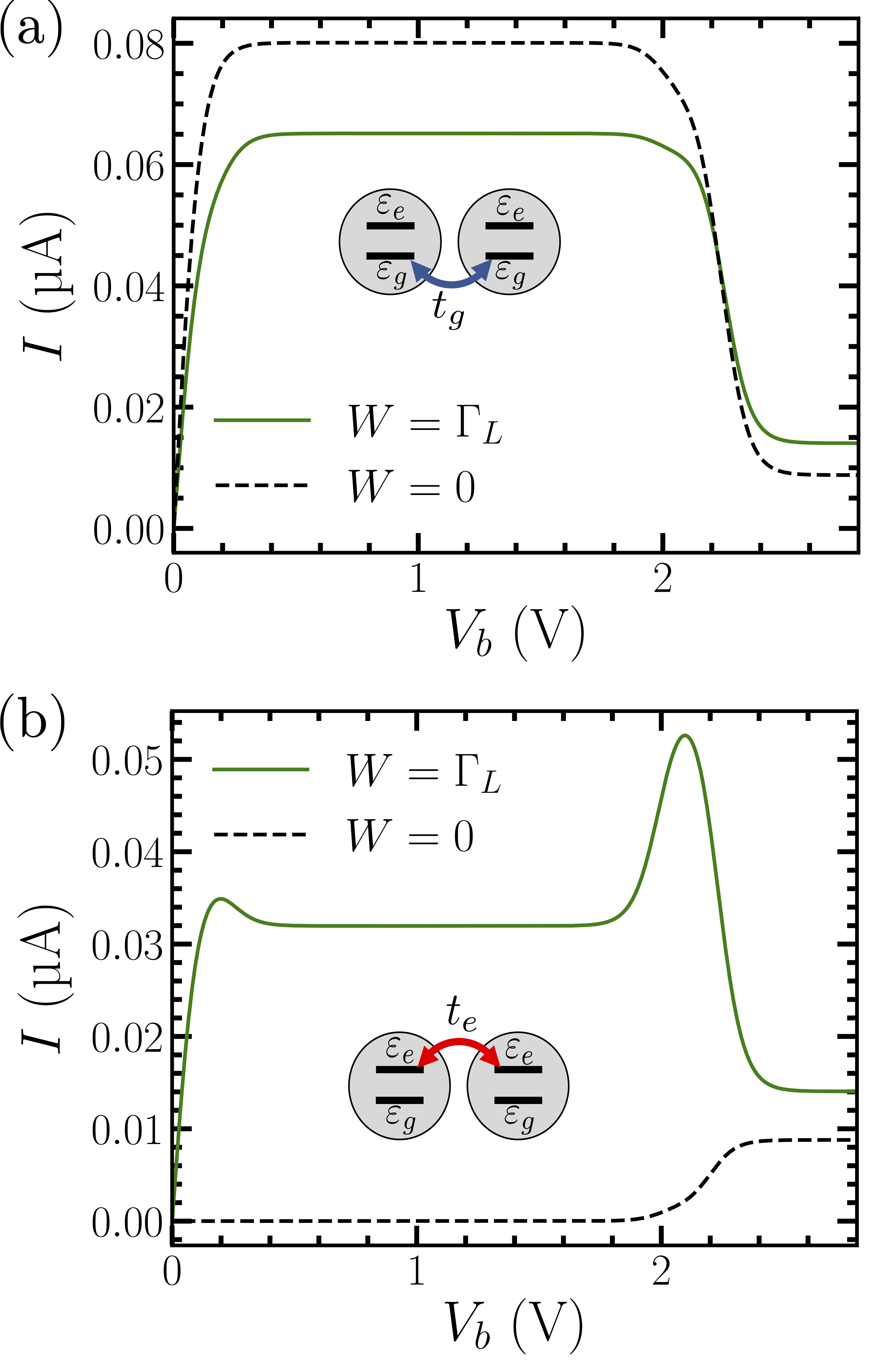
Figure 5: (a) I-V curves for a ground-level conductor ($t_{g}=0.01$ eV) in the presence of incoherent optical pumping (solid line) and without pumping (dashed line). (b) Same as panel (a), for an excited-level conductor ($t_{e}=0.01$ eV). System parameters are given in Table 1.

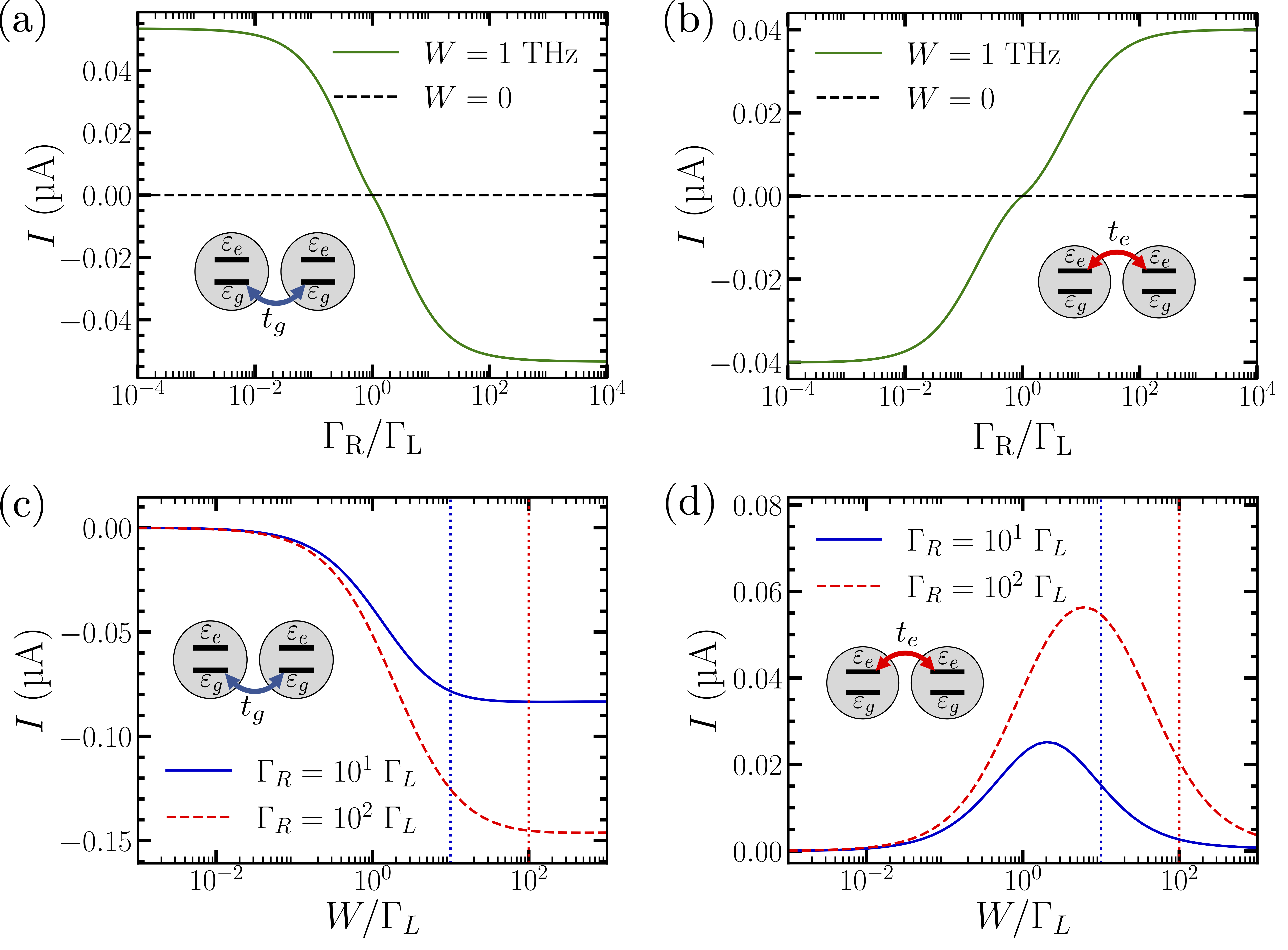
Figure 6: (a) Current at zero bias as a function of the ratio $\Gamma_{R}/\Gamma_{L}$ for different pumping rate $W$, for a ground-level conductor ($t_{g}=0.01$ eV). (b) Same as panel (a), for an excited-level conductor ($t_{e}=0.01$ eV). (c) Current at zero bias as a function of the ratio $W/\gamma_{\rm r}$ for different tunneling rates $\Gamma_{R}/\Gamma_{L}$, for a ground-level conductor ($t_{g}=0.01$ eV). (d) Same as panel (c) for an excited-level conductor ($t_{e}=0.01$ eV). In panels (a) and (b), $\Gamma_{L}=1$ THz while $\Gamma_{R}$ changes. System parameters are given in Table 1.

III.3.2 Incoherently-Driven Conductance

Figure 5 shows the I-V curves for ground and excited level conductors, in the presence of incoherent radiative pumping at rate $W$. For the ground conductor [Fig. 5(a)] incoherent pumping drives electrons out of the delocalized ground eigenstates into the localized excited eigenstates, thus suppressing transport at low bias. At higher bias where excited states become resonant with the leads, pumping enhances transport by moving electrons into excited levels. For excited level conductors [Fig. 5(b)], the current is higher with incoherent driving due to increased population of delocalized states. For the ground and excited level conductors, there is no current at zero bias voltage for zero or finite incoherent pumping rate $W$.

By assuming asymmetric lead transfer rates $\Gamma_{L}\neq\Gamma_{R}$, incoherent illumination induces photocurrents at zero bias ($V_{b}=0$), an effect also predicted in Refs. [28, 29]. This is explored in Figure 6, where photocurrents produced by ground and excited level conductors are shown. For both types of conductors, the currents reach the same magnitude, but electrons move in opposite directions. The direction of the current depends on the type of delocalized states established in the system. For ground level conductors, incoherent pumping empties the delocalized ground eigenstates that receive electrons from the lead with the highest transfer rate, thus producing a photocurrent towards the other contact [Figure 6(a)]. For an excited level conductor, electrons pumped from the local ground to the delocalized excited eigenstates tunnel to the lead with highest transfer rate, producing a photocurrent in that direction [Figure 6(a)].

Figures 6(c) and 6(d) show the photocurrent at zero bias voltage as a function of $W$ for ground and excited level conductors, respectively, for two different transfer ratios $\Gamma_{R}/\Gamma_{L}$. For ground level conductors, the photocurrent is appreciable when $W\gtrsim\Gamma_{L}$, but tends to a constant value when $W\gtrsim\Gamma_{R}$ for both ratios (vertical lines). For excited level conductors, the photocurrent has a maximum at $\Gamma_{L}<W<\Gamma_{R}$, but decreases to zero when $W\gg\Gamma_{R}$ for both ratios (vertical lines).

IV Conclusions

We studied stationary electron transport through a conducting array having one and two sites in the presence of radiative decay, non-radiative relaxation, and incoherent radiative driving. We use a Lindblad quantum master equation to describe the problem, reducing numerical cost and facilitating the physical interpretation of the current-voltage characteristics of the device. Despite its simplicity, the Lindblad theory can reproduce recently reported negative differential conductance measurements in single-molecule junctions [11]. The theory can also qualitatively capture experimentally-relevant phenomena such as current-induced light and light-induced current. The latter occurs even at zero bias as a consequence of the electron tunneling induced by the incoherent pumping source. For a two-site conducting array model with electron tunneling in the ground or excited levels, we showed that the direction of the light-induced currents depends on the type of internal state delocalization present in the system.

Future extensions of the theory that include the coupling of non-conducting degrees of freedom such as nuclear vibrations with quantized electromagnetic fields could be used to address the microscopic mechanism underlying the recently reported modifications of the current-voltage characteristics of conducting arrays in infrared cavities [40], extending previous experiments on organic conductivity in optical microcavities [41, 42, 43, 44, 45] to the THz regime. Further extensions of the open quantum system theory discussed here to include strong polaron effects and non-Markovian system-bath interactions can also be developed building on previous work [24, 27].

Appendix A Derivation of Equations (10) and (11).

Building on the approach from Refs. [31, 46], here we derive general expressions for the electron and photon currents in the system, in terms of populations of the conducting array eigenstates. The electron transfer between the conducting array and the left ($l=L$) or the right ($l=R$) lead is described by the Hamiltonian

$$\hat{\mathcal{H}}=\hat{\mathcal{H}}_{S}+\hat{\mathcal{H}}_{B}+\hat{\mathcal{H}}_{SB},$$ (11)

where the conducting array is described by

$$\hat{\mathcal{H}}_{S}=\sum_{i}\Bigg{[}\sum_{\alpha}\varepsilon_{\alpha}\hat{n}_{i,\alpha}+\frac{U}{2}\sum_{\beta\neq\alpha}\hat{n}_{i,\beta}\hat{n}_{i,\alpha}+\sum_{\alpha}t_{\alpha}\left(\hat{d}_{i,\alpha}^{\dagger}\hat{d}_{i+1,\alpha}+\hat{d}_{i+1,\alpha}^{\dagger}\hat{d}_{i,\alpha}\right)\Bigg{]},$$ (12)

the lead is described by

$$\hat{\mathcal{H}}_{B}=\sum_{k_{l}}\omega_{k_{l}}\hat{c}_{k_{l}}^{\dagger}\hat{c}_{k_{l}},$$ (13)

and the interaction between them is described by

$$\hat{\mathcal{H}}_{SB}=\sum_{\alpha,k_{l}}\left(V_{k_{l}}\hat{d}_{i,\alpha}^{\dagger}\hat{c}_{k_{l}}+V_{k_{l}}^{*}\hat{d}_{i,\alpha}\hat{c}_{k_{l}}^{\dagger}\right).$$ (14)

$\hat{d}_{i,\alpha}$ ($\hat{n}_{i,\alpha}=\hat{d}_{i,\alpha}^{\dagger}\hat{d}_{i,\alpha}$) is the fermionic annihilation operator of electrons in the $i-$th site and energy level $\alpha$ of the conducting array, and $\hat{c}_{k_{l}}$ is the fermionic annihilation operator of electrons in the mode $\omega_{k_{l}}$ of the lead $l$.
The interaction Hamiltonian in Eq. (14) describes the transfer of electron with the lead, creating and annihilating electrons in the conducting array with an associated coupling constant $V_{k_{l}}$ and $V_{k_{l}}^{*}$, respectively. We asumme that the lead $l$ transfer electron just with the $i-$th site. The interaction Hamiltonian can be written in a general form

$$\hat{\mathcal{H}}_{SB}=\hat{\mathcal{S}}\otimes\hat{\mathcal{B}}+\hat{\mathcal{S}}^{\dagger}\otimes\hat{\mathcal{B}}^{\dagger},$$ (15)

in terms of system and reservoir (bath) operators

$$\hat{\mathcal{S}}=\sum_{\alpha}\hat{d}_{i,\alpha}^{\dagger}=\sum_{\epsilon,\epsilon^{\prime}}\bra{\epsilon}\sum_{\alpha}\hat{d}_{i,\alpha}^{\dagger}\ket{\epsilon^{\prime}}\ket{\epsilon}\bra{\epsilon^{\prime}},\hskip 14.22636pt{\rm and}\hskip 14.22636pt\hat{\mathcal{B}}=\sum_{k_{l}}V_{k_{l}}\hat{c}_{k_{l}},$$ (16)

respectively. $\hat{\mathcal{S}}$ is written in terms of the system eigenbasis $\omega_{\epsilon}$ and $\ket{\epsilon}$, which satisfies $\hat{\mathcal{H}}_{S}=\sum_{\epsilon}\omega_{\epsilon}\ket{\epsilon}\bra{\epsilon}$.

We adopt an open-quantum system approach for the dynamics between the lead $l$, as an electron bath, and the conducting array, as the system. In the Born approximation, the total density matrix is written as a product $\hat{\rho}=\hat{\rho}_{S}\otimes\hat{\rho}_{B}$ of the reduced system density matrix $\hat{\rho}_{S}$ for the conducting array and the bath density matrix $\hat{\rho}_{B}$ for electrons in the lead. In the weak-coupling regime for $V_{k_{l}}$, the Markovian evolution of the number operator of electrons in the lead $\hat{\mathcal{N}}_{l}=\sum_{k_{l}}\hat{c}_{k_{l}}^{\dagger}\hat{c}_{k_{l}}$ is given by [33]

$$\frac{\rm d}{\rm dt}\langle\hat{\mathcal{N}}_{l}\rangle={\rm Tr}\Bigg{\{}\hat{\mathcal{N}}_{l}\frac{{\rm d}\tilde{\rho}}{\rm dt}\Bigg{\}}=-\int_{0}^{\infty}d\tau\hskip 2.84544pt{\rm Tr}\Big{\{}\hat{\mathcal{N}}_{l}\left[\tilde{\mathcal{H}}_{SB}(t),\left[\tilde{\mathcal{H}}_{SB}(t-\tau),\tilde{\rho}(t)\right]\right]\Big{\}},$$ (17)

where $\tilde{\rho}(t)=\hat{U}(t)\hskip 2.84544pt\hat{\rho}\hskip 2.84544pt\hat{U}^{\dagger}(t)$ and $\tilde{\mathcal{H}}_{SB}(t)=\hat{U}(t)\hskip 2.84544pt\hat{\mathcal{H}}_{SB}\hskip 2.84544pt\hat{U}^{\dagger}(t)$ are in the interaction picture with respect to $\hat{\mathcal{H}}_{0}=\hat{\mathcal{H}}_{S}+\hat{\mathcal{H}}_{B}$ using $\hat{U}(t)=\exp(i\hat{\mathcal{H}}_{0}t)$.
Using the interaction Hamiltonian in Eq. (15), the Eq.(17),

$$\begin{split}\frac{{\rm d}}{\rm dt}\langle\hat{\mathcal{N}}_{l}\rangle=-\int_{0}^{\infty}d\tau\hskip 2.84544pt\Big{[}&\langle\hat{\mathcal{S}}\tilde{\mathcal{S}}^{\dagger}(-\tau)\rangle\langle\hat{\mathcal{N}}_{l}\hat{\mathcal{B}}\tilde{\mathcal{B}}^{\dagger}(-\tau)\rangle+\langle\hat{\mathcal{S}}^{\dagger}\tilde{\mathcal{S}}(-\tau)\rangle\langle\hat{\mathcal{N}}_{l}\hat{\mathcal{B}}^{\dagger}\tilde{\mathcal{B}}(-\tau)\rangle\\ -&\langle\tilde{\mathcal{S}}^{\dagger}(-\tau)\hat{\mathcal{S}}\rangle\langle\tilde{\mathcal{B}}^{\dagger}(-\tau)\hat{\mathcal{N}}_{l}\hat{\mathcal{B}}\rangle-\langle\tilde{\mathcal{S}}(-\tau)\hat{\mathcal{S}}^{\dagger}\rangle\langle\tilde{\mathcal{B}}(-\tau)\hat{\mathcal{N}}_{l}\hat{\mathcal{B}}^{\dagger}\rangle\\ -&\langle\hat{\mathcal{S}}^{\dagger}\tilde{\mathcal{S}}(-\tau)\rangle\langle\hat{\mathcal{B}}^{\dagger}\hat{\mathcal{N}}_{l}\tilde{\mathcal{B}}(-\tau)\rangle-\langle\hat{\mathcal{S}}\tilde{\mathcal{S}}^{\dagger}(-\tau)\rangle\langle\hat{\mathcal{B}}\hat{\mathcal{N}}_{l}\tilde{\mathcal{B}}^{\dagger}(-\tau)\rangle\\ +&\langle\tilde{\mathcal{S}}(-\tau)\hat{\mathcal{S}}^{\dagger}\rangle\langle\tilde{\mathcal{B}}(-\tau)\hat{\mathcal{B}}^{\dagger}\hat{\mathcal{N}}_{l}\rangle+\langle\tilde{\mathcal{S}}^{\dagger}(-\tau)\hat{\mathcal{S}}\rangle\langle\tilde{\mathcal{B}}^{\dagger}(-\tau)\hat{\mathcal{B}}\hat{\mathcal{N}}_{l}\rangle\Big{]},\end{split}$$ (18)

is reduced to mean values of system and bath operators. The time-dependent system and bath operators are

$$\tilde{\mathcal{S}}(t)=\hat{U}(t)\hskip 2.84544pt\hat{\mathcal{S}}\hskip 2.84544pt\hat{U}^{\dagger}(t)=\sum_{\epsilon,\epsilon^{\prime}}\bra{\epsilon}\sum_{\alpha}\hat{d}_{i,\alpha}^{\dagger}\ket{\epsilon^{\prime}}\exp(i\omega_{\epsilon,\epsilon^{\prime}}t)\ket{\epsilon}\bra{\epsilon^{\prime}},\hskip 14.22636pt{\rm and}\hskip 14.22636pt\tilde{\mathcal{B}}(t)=\hat{U}(t)\hskip 2.84544pt\hat{\mathcal{B}}\hskip 2.84544pt\hat{U}^{\dagger}(t)=\sum_{k_{l}}V_{k_{l}}\exp(-i\omega_{k_{l}}t)\hat{c}_{k_{l}},$$ (19)

respectively, where $\omega_{\epsilon,\epsilon^{\prime}}=\omega_{\epsilon}-\omega_{\epsilon^{\prime}}$ in the system transition frequency.

Using that the lead $l$ is a thermal equilibrium bath, described by

$$\hat{\rho}_{B}=\frac{\exp\left(-\beta(\hat{\mathcal{H}}_{l}-\mu_{l}\hat{\mathcal{N}}_{l})\right)}{{\rm Tr}\Big{\{}\exp\left(-\beta(\hat{\mathcal{H}}_{l}-\mu_{l}\hat{\mathcal{N}}_{l})\right)\Big{\}}},$$ (20)

at temperature $T$ ($\beta=1/kT$) and chemical potential $\mu_{l}$, and the anticonmmutation relation of fermionic operators,

$$\{\hat{c}_{k_{l}},\hat{c}_{k^{\prime}_{l}}^{\dagger}\}=\delta_{k_{l},k^{\prime}_{l}},\hskip 14.22636pt{\rm and}\hskip 14.22636pt\{\hat{c}_{k_{l}},\hat{c}_{k^{\prime}_{l}}\}=0=\{\hat{c}_{k_{l}}^{\dagger},\hat{c}_{k^{\prime}_{l}}^{\dagger}\}$$ (21)

the mean value of reservoir operators in Eq. (18) reduces the dynamics of the lead number operator to

$$\begin{split}\frac{{\rm d}}{\rm dt}\langle\hat{\mathcal{N}}_{l}\rangle=-\int_{0}^{\infty}d\tau\hskip 2.84544pt\Big{[}&\langle\hat{\mathcal{S}}^{\dagger}\tilde{\mathcal{S}}(-\tau)\rangle C(\tau)-\langle\tilde{\mathcal{S}}(-\tau)\hat{\mathcal{S}}^{\dagger}\rangle\bar{C}(-\tau)-\langle\hat{\mathcal{S}}\tilde{\mathcal{S}}^{\dagger}(-\tau)\rangle\bar{C}(\tau)+\langle\tilde{\mathcal{S}}^{\dagger}(-\tau)\hat{\mathcal{S}}\rangle C(-\tau)\Big{]},\end{split}$$ (22)

where it have been defined the bath correlations

$$C(\tau)=\sum_{k_{l}}|V_{k_{l}}|^{2}f_{l}(\omega_{k_{l}})\exp\left(i\omega_{k_{l}}\tau\right),\\ \hskip 14.22636pt{\rm and}\hskip 14.22636pt\bar{C}(\tau)=\sum_{k_{l}}|V_{k_{l}}|^{2}(1-f_{l}(\omega_{k_{l}}))\exp\left(-i\omega_{k_{l}}\tau\right),$$ (23)

in terms of the fermion density $f_{l}(\omega)=(\exp{((\omega-\mu_{l})/T_{0})}+1)^{-1}$.

Writing $\hat{\mathcal{S}}$ and $\hat{\mathcal{S}}(-\tau)$ in terms of eigenstates as in Eq. (16) and Eq. (19), respectively, the mean value of system operators in Eq. (22) can be written in terms of system eigenstate population $\rho_{\epsilon,\epsilon}\equiv\langle\epsilon|\hat{\rho}_{S}\ket{\epsilon}$ as

$$\begin{split}\langle\hat{\mathcal{S}}^{\dagger}(-\tau)\hat{\mathcal{S}}\rangle=\sum_{\epsilon,\epsilon^{\prime}}|\bra{\epsilon}\sum_{\alpha}\hat{d}_{i,\alpha}^{\dagger}\ket{\epsilon^{\prime}}|^{2}\exp(i\omega_{\epsilon,\epsilon^{\prime}}\tau)\rho_{\epsilon^{\prime},\epsilon^{\prime}},\hskip 14.22636pt\langle\hat{\mathcal{S}}^{\dagger}\hat{\mathcal{S}}(-\tau)\rangle=\sum_{\epsilon,\epsilon^{\prime}}|\bra{\epsilon}\sum_{\alpha}\hat{d}_{i,\alpha}^{\dagger}\ket{\epsilon^{\prime}}|^{2}\exp(-i\omega_{\epsilon,\epsilon^{\prime}}\tau)\rho_{\epsilon^{\prime},\epsilon^{\prime}},\\ \langle\hat{\mathcal{S}}(-\tau)\hat{\mathcal{S}}^{\dagger}\rangle=\sum_{\epsilon,\epsilon^{\prime}}|\bra{\epsilon}\sum_{\alpha}\hat{d}_{i,\alpha}^{\dagger}\ket{\epsilon^{\prime}}|^{2}\exp(-i\omega_{\epsilon,\epsilon^{\prime}}\tau)\rho_{\epsilon,\epsilon},\hskip 14.22636pt\langle\hat{\mathcal{S}}\hat{\mathcal{S}}^{\dagger}(-\tau)\rangle=\sum_{\epsilon,\epsilon^{\prime}}|\bra{\epsilon}\sum_{\alpha}\hat{d}_{i,\alpha}^{\dagger}\ket{\epsilon^{\prime}}|^{2}\exp(i\omega_{\epsilon,\epsilon^{\prime}}\tau)\rho_{\epsilon,\epsilon},\end{split}$$ (24)

in the secular approximation. Using Eq. (24), the Eq. (22) becomes

$$\begin{split}\frac{{\rm d}}{\rm dt}\langle\hat{\mathcal{N}}_{l}\rangle=\sum_{\epsilon,\epsilon^{\prime}}|\bra{\epsilon}\sum_{\alpha}\hat{d}_{i,\alpha}^{\dagger}\ket{\epsilon^{\prime}}|^{2}\int_{0}^{\infty}d\tau\hskip 2.84544pt\Big{[}&\rho_{\epsilon,\epsilon}\{\bar{C}(\tau)\exp(i\omega_{\epsilon,\epsilon^{\prime}}\tau)+\bar{C}(-\tau)\exp(-i\omega_{\epsilon,\epsilon^{\prime}}\tau)\}\\ -&\rho_{\epsilon^{\prime},\epsilon^{\prime}}\{C(\tau)\exp(i\omega_{\epsilon,\epsilon^{\prime}}\tau)+C(-\tau)\exp(-i\omega_{\epsilon,\epsilon^{\prime}}\tau)\}\Big{]}.\end{split}$$ (25)

Using the principal value theorem, the integrals in Eq. (25),

$$\int_{0}^{\infty}d\tau\hskip 2.84544ptC(\pm\tau)\exp\left(\mp i\omega_{\epsilon,\epsilon^{\prime}}\tau\right)=\frac{1}{2}\Gamma_{l}f_{l}(\omega_{\epsilon,\epsilon^{\prime}}),\hskip 14.22636pt{\rm and}\hskip 14.22636pt\int_{0}^{\infty}d\tau\hskip 2.84544pt\bar{C}(\pm\tau)\exp\left(\pm i\omega_{\epsilon,\epsilon^{\prime}}\tau\right)=\frac{1}{2}\Gamma_{l}\left(1-f_{l}(\omega_{\epsilon,\epsilon^{\prime}})\right),$$ (26)

are reduced to transfer rate $\Gamma_{l}(\omega)=\sum_{k_{l}}|V_{k_{l}}|^{2}\delta(\omega-\omega_{k_{l}})$ and fermion densities $f_{l}(\omega_{\epsilon,\epsilon^{\prime}})$ evaluated at $\omega_{\epsilon,\epsilon^{\prime}}$. In Eq. (26) we consider the transfer rate is constant and neglect lamb-shifts. Using Eq. (26), Eq. (25) is reduced to Eq. (8) in the main text,

$$\frac{\rm d}{\rm dt}\langle\hat{\mathcal{N}}_{l}\rangle=\Gamma_{l}\sum_{\epsilon,\epsilon^{\prime}}|\bra{\epsilon}(\hat{d}^{\dagger}_{i,g}+\hat{d}^{\dagger}_{i,e})\ket{\epsilon^{\prime}}|^{2}\Big{(}(1-f_{l}(\omega_{\epsilon,\epsilon^{\prime}}))\rho_{\epsilon,\epsilon}-f_{l}(\omega_{\epsilon,\epsilon^{\prime}})\rho_{\epsilon^{\prime},\epsilon^{\prime}}\Big{)}.$$ (27)

We use the same methodology for deriving Eq. (9) in the main text for the Markovian evolution of the number of photons in the EM field $\hat{\mathcal{N}}_{\rm r}$, taking into account the commutation relation of bosonic operators of photons.