Prospects of measuring Gamma-ray Burst Polarisation with the Daksha mission

Abstract

The proposed Daksha mission comprises of a pair of highly sensitive space telescopes for detecting and characterising high-energy transients such as electromagnetic counterparts of gravitational wave events and gamma-ray bursts (GRBs). Along with spectral and timing analysis, Daksha can also undertake polarisation studies of these transients, providing data crucial for understanding the source geometry and physical processes governing high-energy emission. Each Daksha satellite will have 340 pixelated Cadmium Zinc Telluride (CZT) detectors arranged in a quasi-hemispherical configuration without any field-of-view collimation (open detectors). These CZT detectors are good polarimeters in the energy range 100 – 400 keV, and their ability to measure polarisation has been successfully demonstrated by the Cadmium Zinc Telluride Imager (CZTI) onboard AstroSat. Here we demonstrate the hard X-ray polarisation measurement capabilities of Daksha and estimate the polarisation measurement sensitivity (in terms of the Minimum Detectable Polarisation: MDP) using extensive simulations. We find that Daksha will have MDP of $30\%$ for a fluence threshold of $10^{-4}$ $\mathrm{erg~{}cm}^{-2}$ (in 10 – 1000 keV). We estimate that with this sensitivity, if GRBs are highly polarised, Daksha can measure the polarisation of about five GRBs per year.

*Suman Bala, sumanbala2210@gmail.com
*Sujay Mate, sujay.mate@tifr.res.in
* These authors contributed equally to this work.

1 Introduction

Gamma-Ray Bursts [(1), GRBs] are the most energetic explosions in the Universe. The initial brief and intense gamma-ray flash originates close to the burst site and is known as the prompt emission. When burst ejecta collides with the external ambient medium, it produces the afterglow emission, which radiates in all wavelengths (radio to gamma-rays) (Rees1992, ; piran05, ; meszaros06, ). GRBs are classified into two categories depending upon the duration of the prompt emission phase and they originate from two different progenitors. Short GRBs are produced by the merger of two compact objects, such as binary neutron stars (BNS) or a neutron star-black hole (NS-BH) pair (eichler89, ; narayan92, ; Abbott_170817A, ), whereas long GRBs originate from the core collapse of massive stars (woosley93, ; iwamoto98, ; macfadyen99, ). In both cases, the central engine is believed to be either a black hole (woosley93, ; iwamoto98, ; macfadyen99, ) or a hyper-massive magnetar (eichler89, ; narayan92, ), that is thought to emit a relativistic jet giving rise to the GRB.

We have a broad understanding of GRBs, but many detailed questions regarding the nature of the central engine and the emission from the relativistic jet still remain unanswered (kumar15, ; zhang19, ). There are competing models regarding the exact energy dissipation process, radiation mechanism, and radiation transfer processes in the prompt emission phase (Gill_etal_2021_review, ). It is well established that these combined processes produce a non-thermal spectrum, often fitted with various phenomenological models like a power law, power law with an exponential cutoff, Band function, etc. (band1993batse, ; gruber2014fermi, ). Most of the spectral analyses show similar fit statistics when fitted with different physical and empirical models (iyyani15, ; Zhang2016, ) ; however, different physical models predict different degrees of polarization. Hence a statistical analysis of polarisation properties of the GRB prompt emission phase can be a very useful tool to constrain the models and answer questions regarding the emission mechanism and geometry of GRB jets (toma08, ; covino16, ; mcconnell16, ; gill18, ; Gill_etal_2021_review, ).

High-energy polarisation measurement is a very photon-hungry task. Due to the short-lived nature of the prompt emission phase, it has been extremely difficult to measure polarisation of GRBs. Polarisation measurements exits only for $\sim 40$ GRBs out of $>5000$ GRBs detected so far. The majority of these detections have come only in the last few years with POLAR (zhang19, ; Kole2020, ) and AstroSat/CZTI (chattopadhyay19, ; Chattopadhyay2022, ) leading the numbers and other missions like BATSE (Willis2005, ), GAP (Yonetoku2012, ) and INTEGRAL/SPI (Gotz09, ; Gotz13, ) contributing to a few measurements. However, different missions have measured different levels of polarisation in the observed GRBs. For example, GAP and INTEGRAL have measured high levels of polarisation (polarisation fraction or degree $>60\%$) in their sample; while POLAR and AstroSat measurements find a low level of polarisation in their sample. In a few cases, POLAR (Burgess2019, ; zhang19, , GRB170114A) and AstroSat/CZTI (Sharma2019, , GRB160821A) have also detected a temporal evolution of polarisation fraction, asserting the highly dynamic nature of the prompt emission. A detailed summary of GRB polarisation measurements can be found in Gill2021 .

The limited number of measurements and low level of observed polarisation in many GRBs necessitates the need for more sensitive and dedicated GRB polarimeters. In the upcoming years, dedicated GRB polarimeters such as POLAR-2 (DeAngelis, ), COSI (Tomsick2022, ) and LEAP (McConnell2021, ) have been proposed to obtain more sensitive polarisation measurements. One such addition to this era would be the proposed high-energy transient mission Daksha (Bhalerao2022a, ; Bhalerao2022b, ). When launched, it will be one of the the most sensitive high-energy telescope in the world that can also perform hard X-ray polarisation measurements. Here we present the expected hard X-ray polarisation sensitivity of Daksha.

This article is organised as follows: In Section 2, we give an overview of the Daksha mission. In Section 3, we briefly explain the polarisation measurement principle Daksha detectors will utilise. In Section 4, we give details of the mass model used to carry out simulations necessary for the sensitivity analysis described in the article. In Section 5, we describe the method that Daksha will use to measure hard X-ray polarisation. In Section 6, we present the sensitivity results, and in Section 7 we summarise and conclude our analysis.

2 The Daksha mission

Daksha is a proposed Indian high-energy transient mission dedicated to studying electromagnetic counterparts of gravitational waves (EMGW) and GRBs (Bhalerao2022a, ). Apart from its primary science goals, Daksha will also detect flares from magnetars, possible counterparts of Fast Radio Bursts (FRBs), outbursts from bright X-ray binaries and Active Galactic Nuclei (AGNs), hard X-ray emissions from the Sun and also Terrestrial Gamma-ray Flashes (TGFs). The details about the science goals of Daksha can be found in Bhalerao2022b .

Daksha consists of two identical satellites on opposite sides of the Earth in a Low Earth Orbit (LEO). Each satellite will cover a broad energy range (1 keV – 1 MeV) and monitor nearly the entire sky. It will be able to detect transients onboard and send alerts over the General Coordinates Network (GCN) within a few minutes of detection. Three types of detectors are used to span the entire energy range: Silicon Drift Diodes (SDDs) form Low Energy (LE) packages to cover the 1 – 30 keV range; Cadmium Zinc Telluride (CZT) detectors form Medium Energy (ME) packages to cover the 20 – 200 keV range; and lastly Sodium Iodide (NaI) scintillators coupled with Silicon Photo-multipliers (SiPM) cover the 100 – 1000 keV range. The current design of Daksha is shown in Figure 1, and more information about instrument details can be found in Bhalerao2022a .

The hemispherical arrangement of 13 ME and LE packages each gives nearly uniform coverage of half the sky. Photons from a GRB located in this half will be incident on multiple faces, all at varying angles. In the medium energy range, the sensitivity is extended to the remaining half of the sky by 4 sunward pointing ME packages.

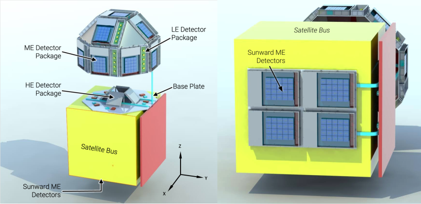
Figure 1: The design of a single Daksha satellite. Left: The payload showing 13 Low-energy (LE) and Medium-energy (ME) detector packages installed on dome-shaped frame with 13 surfaces. The four High-energy (HE) detector packages and the processing electronics are mounted inside the dome. The satellite reference frame is indicated on the bottom right. The $\theta=0^{\circ}$ and $\phi=0^{\circ}$ corresponds to the +ve Z-axis direction while $\theta=0^{\circ}$ and $\phi=90^{\circ}$ corresponds to the +ve Y-axis direction. Right: In addition to the 13 ME packages on the dome, four ME packages are mounted under the satellite bus. Left figure from Bhalerao2022a .

3 Hard X-ray polarimetry with CZT detectors

A single ME package onboard Daksha contains 20 CZT detectors in a 4$\times$5 grid with each detector having size 39.06$\times$39.06$\times$5 mm³. Each detector has 256 pixels of size $\sim$2.46$\times$2.46 mm² with thickness of 5 mm. The small pixel size ($\sim 2.5$ mm) and relatively large thickness (5 mm) of Daksha CZT detectors make them good hard X-ray polarimeters that work on the principle of Compton scattering. The polarimetric capabilities of these detectors have been discussed and demonstrated before on AstroSat/CZTI (chattopadhyay14, ; vadawale17, ; Vaishnava2022, ). Here we give a brief overview of the principle for completeness.

When a photon undergoes Compton scattering, it is scattered preferentially in the direction perpendicular to the direction of the polarisation vector (i.e. direction perpendicular to the electric field vector). Above the incident energy of $\sim$100 keV, Compton scattering interactions in the CZT detector can create two-pixel events where one pixel acts as a scatterer while the other acts as an absorber. The scattered photon has lower energy than the incident photon, leading to a lower mean free path within the detector. Given the pixel size, this scattered photon is likely to get absorbed in one of the adjacent pixels. A small fraction of scattered photons get absorbed in the next-neighboring pixels, considering them increases the chance coincidence probability and hence are not considered for this analysis. These “Compton event” pair positions can be mapped onto a square grid of 3$\times$3 pixels, with the central pixel being the scattering pixel and the surrounding pixels being the absorber pixels. For a square geometry, we get an azimuthal histogram of eight angular bins, each separated by 45^∘ (Figure 2). The modulation observed in this histogram gives us the degree of polarisation (Polarisation Fraction, PF hereafter) and the angle of polarisation (Polarisation Angle, PA hereafter) (chattopadhyay14, , for more details).

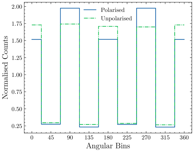
Figure 2: An example of a simulated azimuthal histograms created from the Compton event pairs detected from a modelled CZT detector. The blue curve represents the observed modulation in case of polarised photons while the green curve shows the modulation in case of unpolarised photos.

Apart from Compton scattering, other effects such as chance coincidence, fluorescence and escape peak event pairs can also generate two-pixel events. Hence a selection criteria is needed to separate out possible Compton events from all the two pixel events. We employ the same criteria as described by chattopadhyay14 to select the Compton events. This criteria was decided by running GEANT4 simulations and using Compton kinematics cut on energies. The criteria, applied to both background and GRB events, are as follows:

• To be considered a two pixel event, the two events must have the same time stamp at the microsecond timing resolution of Daksha.

• The events should occur in two adjacent pixels.

• The pixel with lower energy deposit is assumed to be the scattering pixel ($\mathrm{E_{scat}}$) while the other pixel is assumed to be the absorber ($\mathrm{E_{abs}}$) and the energy ratio $\mathrm{E_{abs}/E_{scat}}$ should be between 1 and 6.

• The total energy deposited in both pixels combined (i.e. $\mathrm{E_{scat}+E_{abs}}$) should be between 100 and 400 keV.

A standard method to determine the PA and PF is by fitting a cosine function to the observed azimuthal histogram (Weisskopf2010, ; chattopadhyay14, ; chattopadhyay19, ; Chattopadhyay2022, ). However, there is an inherent asymmetry for sources that are off-axis relative to the detector boresight (as will be the case for most GRBs observed by a single ME package), and the distribution of counts in the azimuthal bins is not strictly sinusoidal (Muleri2014, ). Fitting a cosine to such a distribution leads to systematic errors in determining the PA and PF. In order to avoid the systematics that can arise from the modulation fitting, we choose the template matching approach used by Vaishnava2022 and zhang19 for the analysis carried out in this article (see Section 5 for more details). The templates are generated such that they span entire PA – PF parameter space and are fitted with the observed data to measure the source PA and PF. To generate such templates, we undertake extensive simulations using a detailed chemical and geometrical model (called “mass model”) of the instrument, in this case, the ME packages and the Daksha payload. The following section describes the mass model used for our analysis. The details of the template matching method and sensitivity analysis are described in Section 5 and Section 6 respectively.

4 Daksha mass model

We use the popular Monte-Carlo particle-matter interaction simulation toolkit GEANT4 (Agostinelli2003, ) to perform Daksha mass model simulations. This section briefly details the prototype mass model and its implementation in GEANT4. Some refinements will be made in this mass model when the final payload design is frozen, but the current model includes all the critical components that will affect the polarization measurements. Before giving more details, we first define some of the GEANT4 terminologies that are needed to describe the mass model. In the discussion below, the term event refers to a simulation of a single photon starting with its creation and its propagation through the geometry until it (and all the other secondary particles generated by it) is stopped or leaves the simulation volume. A run refers to a collection of all events that have the same input properties, i.e. photons drawn from an identical spectral (mono-energy or Band function etc.), angular and spatial distribution.

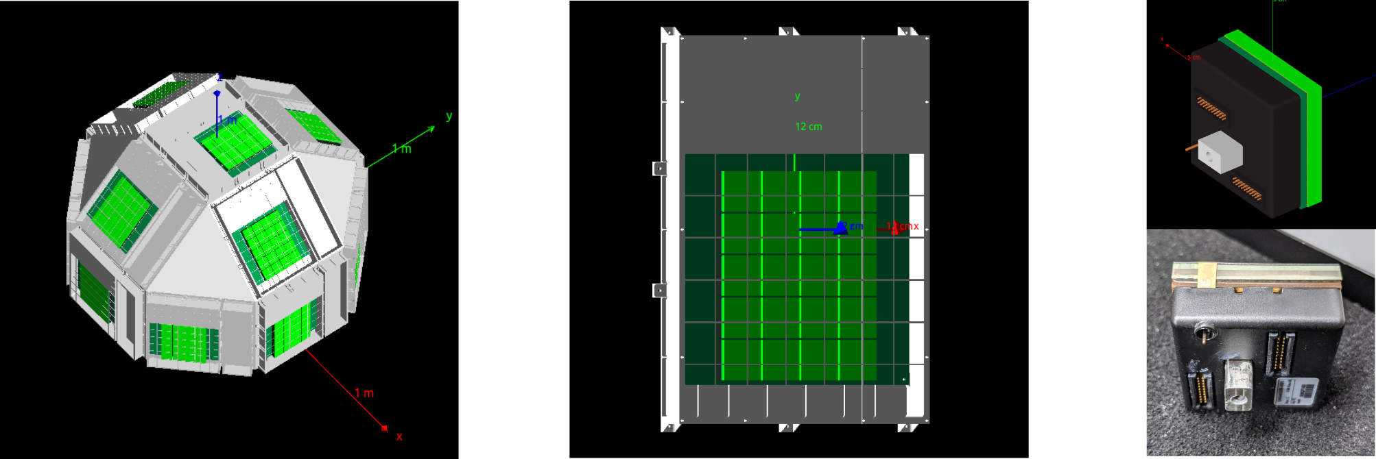
Figure 3: GEANT4 rendering of Daksha mass model and its components. Left: The complete prototype model with 13 ME packages, 13 LE packages without the active volume, and the support dome. The 4 HE packages are not visible here as they are inside the dome. Middle: A single ME package with 20 CZT detector modules (light green squares), the front end PCB (dark green), and the support box with a top lid (grey). Right: A single CZT detector module rendering (top) and a photograph of a real detector module (bottom) for comparison to highlight the accuracy of modelling.

4.1 Geometry

Figure 3 shows the GEANT4 rendering of the prototype Daksha mass model and some of its sub-components. The current version consists of 13 ME packages and 13 LE packages (without the SDD detector volume) in the current configuration, four HE packages in the current configuration, and the support dome. The satellite bus has not been finalised and hence is not included in this simulation. To ensure that this does not affect our results, we are only considering GRBs in the top hemisphere.

The most critical component for our analysis, the single CZT detector module, has been modelled to a mass accuracy of better than 5%, and the model includes most of the internal components (e.g., the Application Specific Integrated Circuit (ASIC) board, heat sink, front end Printed Circuit Board; PCB). For PCBs, individual components are not modelled and they are modelled as sheet of equivalent mass and a typical PCB composition (Hanafi2012, ). For the HE package, only the NaI active volume and the Aluminium shield around the volume have been modelled. Other components like the SiPMs do not have enough material to significantly affect our simulations, but would add computational burden, hence they have been excluded.

4.2 Physics and Tracking

The simulation currently only tracks electromagnetic interactions between 250 eV to 100 GeV using the built-in G4LivermorePolarisedPhysics physics list. Atomic de-excitation is activated to produce secondary particles via fluorescence and Auger electron escape.

We have used the sensitive detector approach of GEANT4 to track the interactions in the active volume. The CZT volume has been divided into 256 pixels, and each pixel acts as an individual sensitive detector. All the electrons produced by the primary (or secondary) photon are tracked along with their energy deposits until they are stopped. If these electrons deposit non-zero energy in a pixel volume, the energy deposit is accumulated and the total energy deposit in that pixel is returned at the end of every event.

4.3 Input and output

The G4GeneralParticleSource class is used to generate input photons. The input characteristics of photons (e.g. spectral, positional, and angular distribution) are defined using the standard GEANT4 input macro files. Currently, a planar or isotropic source with either mono energy or custom input spectra are used depending upon the simulation configuration (see Sections 5.1,  6.2.1 and 6.2.2).

The output of a single run is a FITS file similar to the “time-tagged event files (TTE)” produced by many X/gamma-ray instruments operating in the event mode. The file stores the event ID of the detected event (this is equivalent to event time that is stored in case of the real data), the deposited energy, and the pixel in which the event is detected. In case of multiple events, all the pixels with non-zero energy deposits are recorded individually with the same eventID. Along with the event info, all the metadata related to the run is stored in the header of the FITS extension. This includes input source geometry, the spectral and angular distribution of photons, and the input seeds to allow full reproducibility of any simulation.

5 Polarimetry using template matching

As mentioned in Section 3, we use the template matching method to measure the PA and PF from the observed azimuthal histogram. The method compares (using $\chi^{2}$ statistics) the observed azimuthal histogram with a library of pre-computed template histograms corresponding to different PA and PF values. The following two subsections describe the steps involved in creating the library of templates and the basic principle of the template matching method.

5.1 Template azimuthal histogram generation

The template matching method requires a template bank that spans the entire PA/PF parameter space. The template bank can be created by simulating 100% polarised histograms at different PAs to cover the PA space and combining them with unpolarised histograms to cover the PF space. We generate the template histogram library by running a set of GEANT4 simulations for a given direction in the sky.

For a single direction, 57 energies between 100 keV to 1 MeV are chosen with increasing step size at higher energies (typically the bin size is $\sim$ energy resolution). The upper limit on the simulation energy is decided by doing a convergence analysis such that for a typical Band spectrum, the Poisson uncertainty in 100 — 400 keV is $\lesssim$1%. For each energy, 18 simulations with 100% polarised input photons are carried out by varying the polarisation angle in steps of 10^∘ from 0^∘ to 170^∘. By carrying out a limited number of simulations with finer PA spacing, we found that the number of photons in each of the eight azimuthal bins varies smoothly with PA, and the variation can be modelled as the sum of a sinusoid and its second harmonic. Thus, we can carry out simulations with 10^∘ spacing in PA, and interpolate to calculate the histograms for intermediate angles. Additional simulations with the same energies are carried out with unpolarised input photons from the same incidence direction. In total, for a given source direction, we run $57\times(18+1)=1083$ simulations.

For each simulation, we shine 5$\times$10⁶ photons on the entire mass model. The number is determined by carrying out a convergence estimation such that for the final template the relative error in each azimuthal bin is less than 1%. From these simulations, azimuthal histograms at each energy and polarisation angle are extracted using the criteria explained in Section 3.

For a source (GRB in our case) with incident spectra $S(E)$, where $E$ is the photon energy, the azimuthal histograms at each PA are co-added in the energy space by weighting them with $S(E)$. This gives us the 100% polarised azimuthal histograms for the incident source spectra from a given direction. The same spectral scaling is applied for the unpolarised simulations to get the unpolaried histogram for the incident source spectrum.

To create an azimuthal histogram template bank in PA/PF space for the given source, the 100% polarised azimuthal histograms are first interpolated to a 1^∘ grid in PA space, and then they are combined with the unpolarised histograms to generate template azimuthal histograms in PF space (in PF range 0 to 1 in steps of 0.01) using the following relation:

$$H_{i,t}(p,\psi)=p\cdot H_{i,t}(1,\psi)+(1-p)\cdot H_{i,t}(0);\hskip 10.0pt0\leq i<8,$$ (1)

where $H_{i,t}(p,\psi)$ is the template azimuthal histogram for PA=$\psi$ and PF=$p$ grid point ($i$ represents the $i^{\mathrm{th}}$ azimuthal bin and $t$ stands for template histogram), $H_{i,t}(1,\psi)$ is the 100% polarised azimuthal histogram with PA=$\psi$ and $H_{i,t}(0)$ is the unpolarised histogram. A schematic representation of template creation process is shown in the Figure 4.

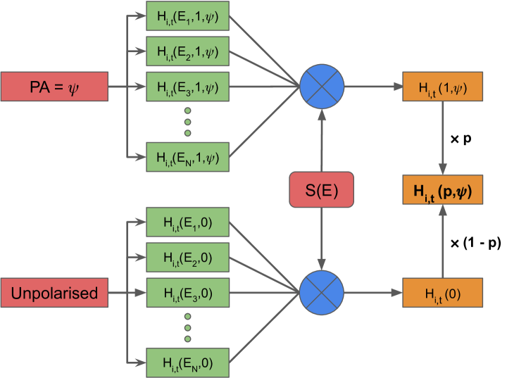
Figure 4: A schematic diagram showing creation of template histogram $H_{i,t}(p,\psi)$ for PA=$\psi$ and PF=$p$. The $H_{i,t}(E,1,\psi)$ represents the 100% polarised template histogram at energy $E$ and PA=$\psi$, $H_{i,t}(E,0)$ represents the unpolarised template histogram at energy $E$. The $S(E)$ represents the GRB spectra. The process is repeated for different PAs and PFs to generate the template bank over the entire PA/PF parameter space.

5.2 Template matching by $\chi^{2}$ minimisation

We use $\chi^{2}$ statistics to quantitatively compare the observed azimuthal histogram with the library of template azimuthal histograms. We define a $\chi^{2}(p,\psi)$ as:

$$\chi^{2}(p,\psi)=\displaystyle\sum_{i=0}^{i=7}\frac{\left[\bar{H}_{i,o}(p,\psi)-\bar{H}_{i,t}(p,\psi)\right]^{2}}{\bar{\sigma}_{i,o}^{2}(p,\psi)+\bar{\sigma}_{i,t}^{2}(p,\psi)}$$ (2)

Where $\bar{H}_{i,o}(p,\psi)$ and $\bar{H}_{i,t}(p,\psi)$ are normalised observed and template histograms for PF value of $p$ and PA value of $\psi$ respectively and $\bar{\sigma}_{i,o}^{2}(p,\psi)$ and $\bar{\sigma}_{i,t}^{2}(p,\psi)$ are errors on them. The normalisation is done by dividing by total number of counts in all eight bins, i.e. by $N=\sum H_{i}$. We simulate our template bank such that $\bar{\sigma}_{i,t}^{2}(p,\psi)<0.01$ and hence in actual estimation of the $\chi^{2}(p,\psi)$ we neglect the $\bar{\sigma}_{i,t}^{2}(p,\psi)$ term. The $\chi^{2}(p,\psi)$ is estimated individually for each ME package on all 13 faces of Daksha. As observed counts on each face are independent, we add the $\chi^{2}(p,\psi)$ values from different faces to estimate the total $\chi^{2}_{tot}(p,\psi)$:

$$\chi^{2}_{tot}(p,\psi)=\displaystyle\sum_{j}\chi^{2}_{j}(p,\psi)$$ (3)

where the sum is evaluated over the face ID $j$. The best-fit values for $p$ and $\psi$ for a given GRB are obtained by minimising the $\chi^{2}_{tot}(p,\psi)$ over the predetermined grid of PA/PF values. The errors on the best-fit parameters are obtained using the confidence contours for a two-parameter $\chi^{2}$ distribution with $\Delta\chi^{2}_{tot}(p,\psi)$ = 2.3, 6.18, and 11.83 corresponding to the confidence levels of 1$\sigma$, 2$\sigma$ and 3$\sigma$ respectively with $\Delta\chi^{2}_{tot}(p,\psi)$ defined as:

$$\Delta\chi^{2}_{tot}(p,\psi)=\chi^{2}_{tot}(p,\psi)-\mathrm{min}(\chi^{2}_{tot}(p,\psi))$$ (4)

For the minimisation process, we only use the top five faces (arranged in a decreasing order of effective area for a given direction) to compute the $\chi^{2}_{tot}(p,\psi)$ as our tests show that adding more faces does not have a significant impact on the results. Hence, for all the analyses described below, only the relevant five faces are used in the template-matching process.

6 Polarimetric sensitivity of Daksha

The most common way to express the sensitivity of a polarimeter is in terms of the “Minimum Detectable Polarisation” (MDP) that can be achieved with it. Formally, MDP is defined as: “The degree of polarization corresponding to the amplitude of modulation that has only a 1% probability of being detected by chance” (Weisskopf2010, ). It is computed as follows:

$$\mathrm{MDP}=\frac{4.29}{\mu_{100}R_{s}}\left[\frac{R_{s}+R_{B}}{T}\right]^{1/2}$$ (5)

where $\mu_{100}$ is the modulation factor for 100% polarised light, $R_{s}$ is the source count rate, $R_{B}$ is the background count rate and $T$ is the total source exposure. However, this is strictly valid only for on-axis incidence as the equation is derived assuming ideal sinusoidal variation (Weisskopf2010, , for derivation). As mentioned in Section 5, the observed modulation is not sinusoidal for off-axis incidence and particularly for the pixellated CZT detectors, hence the above equation is not strictly valid. Therefore to quantify the polarisation measurement sensitivity of Daksha, we use a Monte Carlo-based approach which stems from the basic definition of MDP following the approach presented in Vaishnava2022 . In this section, we describe the Monte Carlo method (called MC-MDP hereafter) used to measure the MDP for Daksha, show the sensitivity results obtained using the MC-MDP, and verify our sensitivity by injecting two GRBs and recovering their polarisation.

6.1 Minimum Detectable Polarisation using Monte Carlo approach

The definition of MDP states that if we repeatedly measure polarisation for an unpolarised source, in 99% of the cases we should measure the PF less than the MDP. In other words, if we measure PF for a large number of realisations of azimuthal histograms from an unpolarised GRB, the 99^th percentile of the measured PF distribution gives the value of MDP for a given source direction and spectrum. The MC-MDP uses this definition to measure MDP for a given polarimeter.

Mathematically, a single realisation of an unpolarised observed azimuthal histogram corresponding to a GRB with fixed spectral parameters and duration $T_{grb}$ can be represented as:

$$H_{i,o}(0)=P(\overline{H}^{grb}_{i}T_{grb})+P(\overline{H}^{bkg}_{i}T_{grb})\\ -P(\overline{H}^{bkg}_{i}T_{bkg})\frac{T_{grb}}{T_{bkg}}$$ (6)

where $P(\lambda)$ represents Poisson random variable with a mean $\lambda$, $\overline{H}^{grb}_{i}$ is the mean (time-averaged, in terms of counts/s) azimuthal histogram (without any background) for an unpolarised GRB of a given fluence, $T_{grb}$ is the GRB duration, $\overline{H}^{bkg}_{i}$ is the mean (time-averaged, in terms of counts/s) background azimuthal histogram and $T_{bkg}$ is the background duration. Using this equation, one can Poisson sample large number of azimuthal histograms and measure the PA/PF value for each realisation. The MDP is then obtained from the cumulative distribution of measured PF values. The mean histograms for GRB and background are sampled by running GEANT4 simulations. The details of the MC-MDP method in case of MDP estimate for Daksha are explained in the next section.

6.2 Minimum Detectable Polarisation computation for Daksha

To estimate MDP for a given fluence and a given incident direction using MC-MDP, we create 20,000 realisations of the “source” azimuthal histograms. Each realisation is then subjected to the template matching fitting explained in Section 5 to get the measured PA and PF values. The cumulative histogram of the PF values obtained from the 20000 realisations is used to estimate the MDP. For this analysis, we fix the $T_{grb}$ to be 30 s and $T_{bkg}$ to be 1000 s. The mean GRB and background histograms are computed from GEANT4 simulations as explained below. A schematic representation of the entire process is shown in Figure 5.

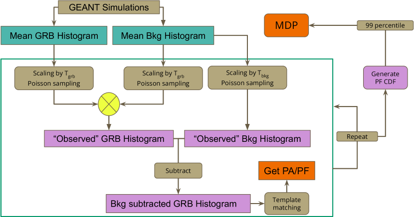
Figure 5: A diagram showing the steps involved in the MC-MDP method that is used to determine MDP for Daksha. The steps in green square are repeated 20,000 times to get the measured PF distribution from unpolarised light which is then used to determine the MDP.

6.2.1 Mean GRB azimuthal histograms

The mean GRB azimuthal histogram is created by shining a large number of unpolarised GRB photons onto the Daksha mass model for a given direction. The input spectra for these simulations follow the Band (band1993batse, ) function with parameters: $\alpha=-1.08$, $\beta=-2.14$, E_peak = 196 keV and norm = 1 ph/cm²/s/keV at 100 keV. We simulate a total of 65,465,240 input photons in the 90 – 1000 keV energy range. The input energy range is fixed to 90 – 1000 keV as we are only interested in the 100 – 400 keV range for the polarisation measurements. From this simulation, we extract the azimuthal histograms as explained in the Section 3 for each of the top five faces of Daksha. These histograms are then scaled appropriately to compute the mean GRB histogram $\overline{H}^{grb}_{i}$.

6.2.2 Mean background azimuthal histograms

The mean background azimuthal histogram is created by shining large number of photons onto the Daksha mass model from the inner surface of a model spherical source of radius of 5 m with a cosine-biased angular distribution to ensure an isotropic flux. The emission angle of photons is restricted between 0^∘ and 6^∘ from the surface normal to the sphere to avoid shinning input photons that do not reach the mass model (Campana2013, , see section 4.2 for details). We only consider photon background components, i.e. Cosmic X-ray Background (CXB), reflection of CXB from Earth’s atmosphere (reflection hereafter) and hard X-ray albedo of Earth (albedo hereafter) as our preliminary study shows that these components are dominant. As CXB and reflection plus albedo have different directional origin, we carry out two different simulations, one with only CXB spectrum as input and one with reflection plus albedo spectrum as input. We assume that Daksha is pointing away from the Earth, i.e. the top face of Daksha is oriented in an opposite direction to the centre of the Earth, and combine both the simulations by weighting them appropriately by expected solid angles. The spectral models for all three components are taken from Cumani2019 . From these simulation, we extract the azimuthal histograms as explained in the Section 3 for each of the top five faces of Daksha. These histograms are then scaled appropriately to compute the mean background histogram $\overline{H}^{bkg}_{i}$.

6.3 Polarisation sensitivity results for Daksha

First, to test the accuracy our method, we compare the MC-MDP with the analytical MDP (Equation 5) for a normal incidence case. For ease of comparison, this test is performed on a single CZT detector module with incident fluence of 10^-3 $\mathrm{erg~{}cm}^{-2}$ in the 10 – 1000 keV range. The comparison is shown in Figure 6.

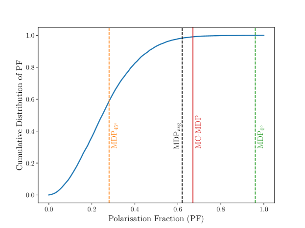
Figure 6: Comparison of MDP value obtained using the MC-MDP method with MDP value obtained using Equation 5 for a normal incidence on a single CZT detector module. The blue curve represents the cumulative distribution (CDF) of the Polarisation Fraction (PF) values obtained from the MC-MDP method. The 99^th percentile of of this CDF gives the MDP (red vertical line). The green and orange vertical lines show the MDP value obtain using the Equation 5 for 0^∘and 45^∘Polarisation Angle (PA), respectively. The MDP depends on PA for the analytical case because the modulation obtained from the pixellated CZT detectors is sensitive to the incident polarisation angle (see Figure 15 in  chattopadhyay14 ). From the figure it can be seen that the MC-MDP is close to the average of the two analytical values (dashed black line).

The reason for two MDP values in the analytical case is because $\mu_{100}$ is a function of PA in case of the pixellated CZT detector and it is minimum for PA = 0^∘ and maximum for PA = 45^∘ (chattopadhyay14, , for more details). It can be seen that the MC-MDP is close to the average of the two analytical values.

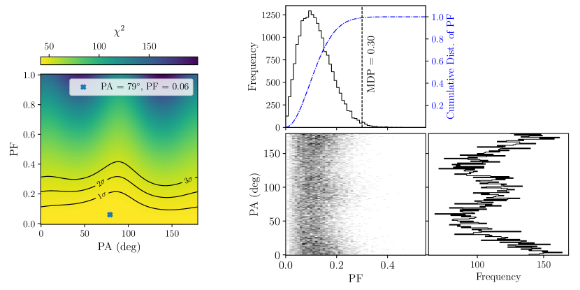
Figure 7: MDP estimation for Daksha ME detectors using the MC-MDP method for a near on-axis incidence ($\theta$ = 5^∘, $\phi$ = 0^∘). The incidence fluence is 10^-4 $\mathrm{erg~{}cm}^{-2}$ in the 10 – 1000 keV range. Left: The $\chi^{2}$ distribution in the PA/PF space obtained from the template matching fit for one realisation of the source azimuthal histogram. The measured value, PA = 79^∘ and PF = 0.06 (corresponding to the minimum $\chi^{2}$), is marked with the blue cross. The $\Delta\chi^{2}$ contours corresponding to 1$\sigma$, 2$\sigma$ and 3$\sigma$ confidence intervals are shown with the black lines. Right: Corner plot for measured PA and PF distribution for all 20,000 realisations of source azimuthal histogram. The probability and cumulative distributions of PF values (marginalised over all PAs) are shown in the top panel of the corner plot. The estimated MDP value of 0.30 is marked with a dashed line.

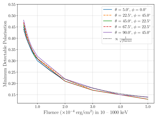
Figure 8: The variation of MDP against the incident GRB fluence for five different off-axis directions with respect to Daksha pointing. As illustrated by the black dashed line, the MDP drops $\propto 1/\sqrt{\mathrm{fluence}}$ (i.e. better sensitivity) as the fluence increases. Due to the symmetry of Daksha, the MDP does not depend strongly on the incident direction. Only five angles are plotted here for clarity, but the other seven follow a similar trend.

The MDP estimate for a near on-axis incidence ($\theta$ = 5^∘ and $\phi$ = 0^∘) for Daksha is shown in Figure 7. The left panel shows the PA/PF contour plot for one azimuthal histogram realisation, and the right panel shows the the final distribution of PA/PF for 20,000 realisations, along with the cumulative histogram of all PF values used to determine the MDP. We estimate an MDP value of 30% with a fluence of 10^-4 $\mathrm{erg~{}cm}^{-2}$ in the 10 – 1000 keV range.

The polarisation sensitivity of a polarimeter is usually correlated with source fluence, i.e., MDP decreases with an increasing GRB fluence. The sensitivity can also be a function of incident direction. To check the MDP dependence on incident direction and fluence, we estimate MDP for Daksha for 12 different incident directions (see Table 1) and 10 different fluence values chosen approximately logarithmically from 5$\times$10^-5 $\mathrm{erg~{}cm}^{-2}$ to 5$\times$10^-4 $\mathrm{erg~{}cm}^{-2}$. The fluences corresponds to typical bright GRBs detected by Fermi/GBM. The 12 directions are chosen in the first half of the first octant of the coordinate sphere ($\theta\in$ [0^∘, 90^∘] and $\phi\in$ [0^∘, 45^∘]) such that they span unique directions in that volume. Given the azimuthal symmetry of Daksha, the results obtained for these directions can be extrapolated to other $\theta,\phi$ in the top hemisphere.

Table 1: Incident directions (in polar coordinates) for which MDP is computed.

$\theta$	$\phi$
0∘	5∘
22.5∘	0∘, 45∘
45∘	0∘, 22.5∘, 45∘
67.5∘	0∘, 22.5∘, 45∘
90∘	0∘, 22.5∘, 45∘

The Figure 8 shows the MDP variation against the incident GRB fluence for five different off-axis directions. It shows that there is no strong dependence of incident direction on MDP thanks to the symmetrical design of Daksha ME packages. The dependence of MDP on fluence shows an expected behaviour, and the MDP drops $\sim 1/\sqrt{\mathrm{fluence}}$ as the fluence increases.

6.4 Validation of polarization measurements

We verify the estimated polarisation sensitivity for Daksha by injecting two GRBs detected by AstroSat/CZTI. The GRBs are chosen such that they have secure measurement of polarisation fraction from current instruments, are above the MDP and fluence threshold of Daksha, and would be detectable (considering orbital parameters) assuming Daksha was active at the time of these events. The spectral and polarimetric parameters for these GRBs are taken from Chattopadhyay2022 . To compute the position of these GRBs in the Daksha frame ($\theta$, $\phi$ in polar coordinates), we use satellite orbit simulations as per the mission profile and convert the celestial coordinates of the GRB into Daksha frame. The spectral and polarimetric parameters of the GRB as well as the calculated $\theta$, $\phi$ are given in Table 2.

Table 2: Injected GRB parameters for the polarisation sensitivity verification.

Name	$\theta$, $\phi$	$\alpha$	$\beta$	Ep	$\Delta$T	Fluence	PF	PA
	(deg)			(keV)	(s)	(erg cm-2)		(deg)
GRB 180103A	90.44, 239.67	-1.31	-2.24	273	165.83	$2.3\times 10^{-4}$	0.71	122.13
GRB 180914B	34.16, 124.08	-0.75	-2.10	453	160.04	$5.99\times 10^{-4}$	0.48	68.41

The results of this test are shown in Figure 9. It can be seen that, for both GRBs, the measured values of PA and PF are close to the injected values and lie well within the 1-$\sigma$ confidence interval. In both cases, the injected PF is above the MDP, indicating Daksha can measure the polarisation properties of a GRB accurately, provided the PF is above the MDP threshold.

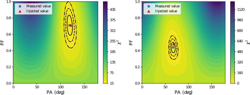
Figure 9: Figure showing measured values of PA and PF for two injected GRBs (GRB 180103A on left and GRB 180914B on right). The solid, dashed and dotted dashed black lines show the 1$\sigma$, 2$\sigma$ and 3$\sigma$ confidence intervals respectively. The injected parameters are given in table 2. For GRB 180103A, the measured PA/PF values are (119^∘$\pm$6^∘, 0.71$\pm$0.12) and for GRB 180914B, the measured PA/PF values are (67^∘$\pm$4^∘, 0.44$\pm$0.06). Daksha can recover the PA and PF accurately for both the GRBs.

Photons for any given GRB have different angles of incidence on each ME package of the payload. This provides us with an excellent opportunity to control any systematic effects that may arise from unknown angle-dependent effects, which will likely average out over the multiple packages. For the brightest bursts, we will also be able to measure the PA and PF from individual ME packages and compare the consistency of the results.

6.5 GRB polarisation measurement rates

Daksha is expected to measure polarisation of about five GRBs per year above the fluence of $10^{-4}$ $\mathrm{erg~{}cm}^{-2}$ if GRBs are highly polarised (PF $>$ 30%). To estimate this rate, we find the number of detected GRBs above the fluence of $10^{-4}$ $\mathrm{erg~{}cm}^{-2}$ by Fermi/GBM in its 14 years of operation. We scale this number by the ratio between the duty cycle of two Daksha satellites and Fermi/GBM and divide it by 14 to obtain the per year rate. Comparing this with AstroSat/CZTI, Daksha will be five times more sensitive. Note that although AstroSat/CZTI has reported 20 GRB polarisation measurements in five years, only five of them have secured polarisation measurements (other 15 are upper limits), giving a polarisation measurement rate of one per year (Chattopadhyay2022, ).

7 Conclusions

The proposed Daksha mission has high sensitivity for detecting Gamma Ray Bursts and other high energy transients. We can exploit the creation of two-pixel events by Compton scattering of incident photons to measure the polarisation of the source in the 100 – 400 keV range. This ability has already been demonstrated on AstroSat/CZTI, and Daksha is poised to surpass CZTI’s polarisation sensitivity.

In this article, we have discussed the method that will be used to measure hard X-ray polarisation using Daksha CZT detectors. The method uses a template matching approach where pre-computed templates (over a grid of PA/PF values) are compared with the observed modulation to measure the polarisation angle (PA) and polarisation fraction (PF) of the source. We have performed detailed GEANT4 simulations using the mass model of Daksha to quantify the polarisation measurement sensitivity of Daksha. The sensitivity has been quoted using the standard Minimum Detectable Polarisation (MDP) metric. To account for the non-normal incidence directions of photons, we have adopted a new Monte-Carlo-based approach to compute the MDP. This method gives consistent results with the analytical formula for on-axis cases, but can be readily generalised to other angles.

Our results show that thanks to the symmetrical design of Daksha, for a given fluence, MDP does not depend strongly on the incident direction (with respect to the satellite pointing), and hence Daksha will have a near-uniform polarisation measurement sensitivity for half of the sky. For a fluence of $10^{-4}$ $\mathrm{erg~{}cm}^{-2}$ in the energy range 10 – 1000 keV, we obtain MDP of 30% for Daksha. Given this sensitivity, we predict that if GRBs are highly polarised, Daksha can confidently measure polarisation for at least five GRBs per year; five times better than AstroSat/CZTI. Daksha is likely to be operational during the same period as other dedicated GRB polarisation missions such as POLAR-2, COSI and LEAP. Given the detection sensitivity and all-sky coverage of Daksha, it will detect many GRBs simultaneously with these missions, and joint analysis of such GRBs will play an important role in understanding the prompt emission. A more detailed analysis of GRB polarisation measurement statistics with Daksha and its implication on breaking the degeneracy in the proposed physical models for prompt emission will be carried out in subsequent works. Overall, when launched, Daksha will play an important role in the field of GRB polarisation.

Softwares

Numpy (numpy, ), Scipy (2020SciPy-NMeth, ), Matplotlib (matplotlib, ), Astropy (2013A&A…558A..33A, ; 2018AJ….156..123A, , http://www.astropy.org),
Ephem  [https://pypi.python.org/pypi/pyephem/], GEANT4 (Agostinelli2003, , https://geant4.web.cern.ch/)

Code, Data, and Materials Availability

The codes are in a continuous state of development and can be made available on a reasonable request to the authors.

References

- (1) R. W. Klebesadel, I. B. Strong, and R. A. Olson, “Observations of Gamma-Ray Bursts of Cosmic Origin,” ApJL 182, L85 (1973).
- (2) M. J. Rees and P. Meszaros, “Relativistic fireballs - Energy conversion and time-scales.,” MNRAS 258, 41 (1992).
- (3) T. Piran, “The physics of gamma-ray bursts,” Reviews of Modern Physics 76, 1143–1210 (2004).
- (4) P. Mészáros, “Gamma-ray bursts,” Reports on Progress in Physics 69, 2259–2321 (2006).
- (5) D. Eichler, M. Livio, T. Piran, et al., “Nucleosynthesis, neutrino bursts and gamma-rays from coalescing neutron stars,” Nature 340, 126–128 (1989).
- (6) R. Narayan, B. Paczynski, and T. Piran, “Gamma-ray bursts as the death throes of massive binary stars,” ApJ 395, L83–L86 (1992).
- (7) B. P. Abbott, R. Abbott, T. Abbott, et al., “Gravitational Waves and Gamma-Rays from a Binary Neutron Star Merger: GW170817 and GRB 170817A,” ApJ 848, L13 (2017).
- (8) S. E. Woosley, “Gamma-ray bursts from stellar mass accretion disks around black holes,” ApJ 405, 273–277 (1993).
- (9) K. Iwamoto, P. A. Mazzali, K. Nomoto, et al., “A hypernova model for the supernova associated with the -ray burst of 25 April 1998,” Nature 395, 672–674 (1998).
- (10) A. I. MacFadyen and S. E. Woosley, “Collapsars: Gamma-Ray Bursts and Explosions in “Failed Supernovae”,” ApJ 524, 262–289 (1999).
- (11) P. Kumar and B. Zhang, “The physics of gamma-ray bursts & relativistic jets,” Phys. Rep. 561, 1–109 (2015).
- (12) S.-N. Zhang, M. Kole, T.-W. Bao, et al., “Detailed polarization measurements of the prompt emission of five gamma-ray bursts,” Nature Astronomy 3, 258–264 (2019).
- (13) R. Gill, M. Kole, and J. Granot, “GRB Polarization: A Unique Probe of GRB Physics,” arXiv e-prints , arXiv:2109.03286 (2021).
- (14) D. Band, J. Matteson, L. Ford, et al., “BATSE Observations of Gamma-Ray Burst Spectra. I. Spectral Diversity,” ApJ 413, 281 (1993).
- (15) D. Gruber, A. Goldstein, V. W. von Ahlefeld, et al., “The fermi gbm gamma-ray burst spectral catalog: four years of data,” The Astrophysical Journal Supplement Series 211(1), 12 (2014).
- (16) S. Iyyani, F. Ryde, B. Ahlgren, et al., “Extremely narrow spectrum of GRB110920A: further evidence for localized, subphotospheric dissipation,” MNRAS 450, 1651–1663 (2015).
- (17) B.-B. Zhang, Z. L. Uhm, V. Connaughton, et al., “SYNCHROTRON ORIGIN OF THE TYPICAL GRB BAND FUNCTION—a CASE STUDY OF GRB 130606b,” The Astrophysical Journal 816, 72 (2016).
- (18) K. Toma, T. Sakamoto, B. Zhang, et al., “Statistical Properties of Gamma-Ray Burst Polarization,” Astrophysical Journal 698, 1042–1053 (2009).
- (19) S. Covino and D. Gotz, “Polarization of prompt and afterglow emission of Gamma-Ray Bursts,” Astronomical and Astrophysical Transactions 29, 205–244 (2016).
- (20) M. L. McConnell, “High energy polarimetry of prompt GRB emission,” New A Rev. 76, 1–21 (2017).
- (21) R. Gill, J. Granot, and P. Kumar, “Linear polarization in gamma-ray burst prompt emission,” MNRAS 491, 3343–3373 (2020).
- (22) M. Kole, N. De Angelis, F. Berlato, et al., “The POLAR gamma-ray burst polarization catalog,” Astron. Astrophys. 644 (2020).
- (23) T. Chattopadhyay, S. V. Vadawale, E. Aarthy, et al., “Prompt Emission Polarimetry of Gamma-Ray Bursts with the AstroSat CZT Imager,” ApJ 884, 123 (2019).
- (24) T. Chattopadhyay, S. Gupta, S. Iyyani, et al., “Hard X-Ray Polarization Catalog for a Five-year Sample of Gamma-Ray Bursts Using AstroSat CZT Imager,” Astrophys. J. 936, 12 (2022).
- (25) D. R. Willis, E. J. Barlow, A. J. Bird, et al., “Evidence of polarisation in the prompt gamma-ray emission from GRB 930131 and GRB 960924,” Astron. Astrophys. 439, 245–253 (2005).
- (26) D. Yonetoku, T. Murakami, S. Gunji, et al., “Magnetic Structures in Gamma-Ray Burst Jets Probed by Gamma-Ray Polarization,” ApJ 758, L1 (2012).
- (27) D. Götz, P. Laurent, F. Lebrun, et al., “Variable Polarization Measured in the Prompt Emission of GRB 041219A Using IBIS on Board INTEGRAL,” Astrophysical Journal Letter 695, L208–L212 (2009).
- (28) D. Götz, S. Covino, A. Fernández-Soto, et al., “The polarized gamma-ray burst GRB 061122,” MNRAS 431, 3550–3556 (2013).
- (29) J. M. Burgess, M. Kole, F. Berlato, et al., “Time-resolved GRB polarization with POLAR and GBM. Simultaneous spectral and polarization analysis with synchrotron emission,” A&A 627, A105 (2019).
- (30) V. Sharma, S. Iyyani, D. Bhattacharya, et al., “Time-varying Polarized Gamma-Rays from GRB 160821A: Evidence for Ordered Magnetic Fields,” ApJ 882, L10 (2019).
- (31) R. Gill, M. Kole, and J. Granot, “GRB polarization: A unique probe of grb physics,” Galaxies 9 (2021).
- (32) N. De Angelis, J. M. Burgess, F. Cadoux, et al., “Development and science perspectives of the POLAR-2 instrument: a large scale GRB polarimeter,” in Proc. Sci., 395 (2022).
- (33) J. A. Tomsick, A. Lowell, H. Lazar, et al., “Soft Gamma-Ray Polarimetry with COSI Using Maximum Likelihood Analysis,” in Handbook of X-ray and Gamma-ray Astrophysics, 73 (2022).
- (34) M. L. McConnell, M. Baring, P. Bloser, et al., “The LargE Area burst Polarimeter (LEAP) a NASA mission of opportunity for the ISS,” in UV, X-Ray, and Gamma-Ray Space Instrumentation for Astronomy XXII, O. H. Siegmund, Ed., Society of Photo-Optical Instrumentation Engineers (SPIE) Conference Series 11821, 118210P (2021).
- (35) V. Bhalerao, S. Vadawale, S. Tendulkar, et al., “Daksha: On Alert for High Energy Transients,” arXiv e-prints , arXiv:2211.12055 (2022).
- (36) V. Bhalerao, D. Sawant, A. Pai, et al., “Science with the Daksha High Energy Transients Mission,” arXiv e-prints , arXiv:2211.12052 (2022).
- (37) T. Chattopadhyay, S. V. Vadawale, A. R. Rao, et al., “Prospects of hard X-ray polarimetry with Astrosat-CZTI,” Experimental Astronomy 37, 555–577 (2014).
- (38) S. V. Vadawale, T. Chattopadhyay, N. P. S. Mithun, et al., “Phase-resolved X-ray polarimetry of the Crab pulsar with the AstroSat CZT Imager,” Nature Astronomy 2, 50–55 (2018).
- (39) C. S. Vaishnava, N. P. S. Mithun, S. V. Vadawale, et al., “Experimental verification of off-axis polarimetry with cadmium zinc telluride detectors of AstroSat-CZT Imager,” J. Astron. Telesc. Instruments, Syst. 8, 038005 (2022).
- (40) M. C. Weisskopf, R. F. Elsner, and S. L. O’Dell, “On understanding the figures of merit for detection and measurement of x-ray polarization,” Space Telescopes and Instrumentation 2010: Ultraviolet to Gamma Ray 7732, 77320E (2010).
- (41) F. Muleri, “On the operation of X-ray polarimeters with a large field of view,” Astrophys. J. 782, 28 (2014).
- (42) S. Agostinelli, J. Allison, K. Amako, et al., “GEANT4 - A simulation toolkit,” Nuclear Instruments and Methods in Physics Research, Section A: Accelerators, Spectrometers, Detectors and Associated Equipment 506, 250–303 (2003).
- (43) J. Hanafi, E. Jobiliong, A. Christiani, et al., “Material recovery and characterization of pcb from electronic waste,” Procedia - Social and Behavioral Sciences 57, 331–338 (2012). International Conference on Asia Pacific Business Innovation and Technology Management.
- (44) A. von Kienlin, C. A. Meegan, W. S. Paciesas, et al., “The Fourth Fermi-GBM Gamma-Ray Burst Catalog: A Decade of Data,” Astrophys. J. 893, 46 (2020).
- (45) R. Campana, M. Feroci, E. Del Monte, et al., “Background simulations for the Large Area Detector onboard LOFT,” Experimental Astronomy 36, 451–477 (2013).
- (46) P. Cumani, M. Hernanz, J. Kiener, et al., “Background for a gamma-ray satellite on a low-Earth orbit,” Experimental Astronomy 47, 273–302 (2019).
- (47) S. van der Walt, S. C. Colbert, and G. Varoquaux, “The NumPy Array: A Structure for Efficient Numerical Computation,” Computing in Science & Engineering 13, 22–30 (2011).
- (48) P. Virtanen, R. Gommers, T. E. Oliphant, et al., “SciPy 1.0: Fundamental Algorithms for Scientific Computing in Python,” Nature Methods 17, 261–272 (2020).
- (49) J. D. Hunter, “Matplotlib: A 2D Graphics Environment,” Computing in Science & Engineering 9, 90–95 (2007).
- (50) Astropy Collaboration, T. P. Robitaille, E. J. Tollerud, et al., “Astropy: A community Python package for astronomy,” A&A 558, A33 (2013).
- (51) Astropy Collaboration, A. M. Price-Whelan, B. M. Sipőcz, et al., “The Astropy Project: Building an Open-science Project and Status of the v2.0 Core Package,” AJ 156, 123 (2018).