Graph Sampling-based Meta-Learning for Molecular Property Prediction

Abstract

Molecular property is usually observed with a limited number of samples, and researchers have considered property prediction as a few-shot problem. One important fact that has been ignored by prior works is that each molecule can be recorded with several different properties simultaneously. To effectively utilize many-to-many correlations of molecules and properties, we propose a Graph Sampling-based Meta-learning (GS-Meta) framework for few-shot molecular property prediction. First, we construct a Molecule-Property relation Graph (MPG): molecule and properties are nodes, while property labels decide edges. Then, to utilize the topological information of MPG, we reformulate an episode in meta-learning as a subgraph of the MPG, containing a target property node, molecule nodes, and auxiliary property nodes. Third, as episodes in the form of subgraphs are no longer independent of each other, we propose to schedule the subgraph sampling process with a contrastive loss function, which considers the consistency and discrimination of subgraphs. Extensive experiments on 5 commonly-used benchmarks show GS-Meta consistently outperforms state-of-the-art methods by 5.71%-6.93% in ROC-AUC and verify the effectiveness of each proposed module. Our code is available at https://github.com/HICAI-ZJU/GS-Meta.

1 Introduction

Drug discovery is of great significance to public health and the development of new drugs is a long and costly process. In the early lead optimization phase, researchers need to select a large number of molecules as candidates and conduct virtual screening to avoid wasting resources on molecules that are unlikely to possess the desired properties Riniker and Landrum (2013); Sliwoski et al. (2014). Recently, deep learning plays an important role in this process, and several deep models have been investigated to predict molecular property Song et al. (2020); Fang et al. (2022, 2023). In the practical settings, only a few molecules can be made and tested in the wet-lab experiments Altae-Tran et al. (2017); Guo et al. (2021). The limited amount of annotated data often hinders the generalization ability of deep learning models in practical applications Bertinetto et al. (2016).

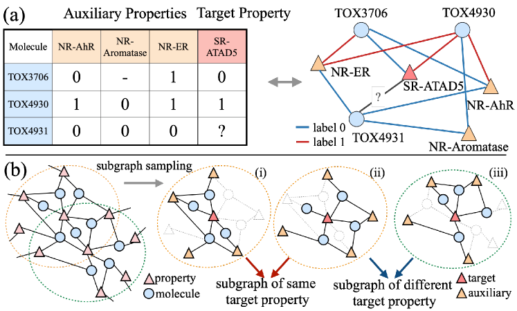
Figure 1: (a) An example of the Molecule-Property relation Graph (MPG) built based on the Tox21 dataset Wu et al. (2018). To predict the SR-ATAD5 property of the TOX4931 molecule, we can utilize some auxiliary properties to form an MPG where molecules and properties are nodes and edges represent property labels (0 or 1). (b) An example of subgraph sampling. Given the MPG, we can sample a pair of subgraphs with the same target property (e.g., (i) and (ii)) as positive samples and another pair with different target properties (e.g., (ii) and (iii)) as negative samples.

Deficient annotated data is often termed a few-shot learning (FSL) problem Wang et al. (2020). Typically, meta-learning Hospedales et al. (2021), which aims to learn how to learn, is used to solve the few-shot problem and several prior works have incorporated meta-learning into molecular property prediction. For example, Meta-GNN Guo et al. (2021) employed a classic meta-learning method, MAML Finn et al. (2017), with self-supervised tasks including bond reconstruction and atom type prediction. Wang et al. constructed a relation graph of molecules and designed a meta-learning strategy to selectively update model parameters.

However, these works have neglected an important fact that, unlike common FSL settings including image classification, a molecule can be observed with multiple properties simultaneously, such as a number of possible side effects. There is also a correlation between different properties, for example, endocrine disorders and cardiac diseases caused by drug side effects may occur together because they share disease pathway Fuchs and Whelton (2020). In predicting the property of a molecule, we can leverage other available labeled properties of the same molecule. When we know some properties of one molecule and are faced with new properties that have fewer labels, we postulate that utilizing these known property labels can alleviate the label insufficiency problem.

To effectively utilize such correlations, we propose a Graph Sampling-based Meta-learning framework, GS-Meta. First, to accurately describe the many-to-many relations among molecules and properties, we build a Molecule-Property relation Graph (MPG), where nodes are molecules and properties, and edges between molecules and properties indicate the label of the molecules in the properties (Figure 1(a)). Second, to employ the inherent graph topology of MPG, we propose to reformulate an episode as a subgraph of MPG, which is composed of a target property node, molecule nodes as well as auxiliary property nodes (Figure 1(b)). Third, in conventional meta-learning Vinyals et al. (2016), episodes are considered to be independently distributed and sampled from a uniform distribution. However, subgraphs are connected in our MPG due to intersecting molecules and edges, they are no longer independent of each other. We propose a learnable sampling scheduler and specify the subgraph dependency in two aspects: (1) subgraphs centered on the same target property node can be seen as different views describing the same task and thus they should be consistent with each other; and (2) subgraphs centered on different target property nodes are episodes of different tasks, and their semantic discrepancy should be enlarged. Hence, we solve this dependency via a contrastive loss function. In short, our contributions are summarized as follows:

• We propose to use auxiliary properties when facing new target property in the few-shot regime and construct a Molecule-Property relation Graph to model the relations among molecules and properties so that the information of the relevant properties can be used through the topology of the constructed graph.

• We propose a Graph Sampling-based Meta-learning framework, which reformulates episodes in meta-learning as sampled subgraphs from the constructed MPG, and schedules the subgraph sampling process with a contrastive loss function.

• Experiments on five benchmarks show that our method consistently outperforms state-of-the-art FSL molecular property prediction methods by 5.71%-6.93% in terms of ROC-AUC.

2 Related Work

Few-shot Learning for Molecules

The few-shot learning (FSL) problem Vinyals et al. (2016); Chen et al. (2019) occurs when there are limited labeled training data per object of interest. Often, meta-learning is used to solve the few-shot learning problem. For example, MAML Finn et al. (2017) learns a good parameter initialization and updates through gradient descents. However, the existing methods are usually investigated for image classification but not tailored to the different settings of molecular property prediction Wang et al. (2021). Recent efforts have been paid to fill this gap. Guo et al. propose to use molecule-specific tasks including masked atoms and bonds prediction to guide the model focus on the intrinsic characteristics of molecules. Wang et al. connect molecules in a homogeneous graph to propagate limited information between similar instances. However, all the prior works have ignored the relationships between molecular properties, i.e., some auxiliary available properties can be used in predicting new molecular properties, and they fail to investigate the relationship.

Episode Scheduler in Meta-learning

Most meta-learning approaches leverage a uniform episode sampling strategy in the training process. To exploit relations between episodes, prior methods have investigated how to schedule episodes to enhance the generalization of meta-knowledge. Liu et al. design a greedy class-pair based strategy rather than uniform sampling. Fei et al. consider the relationship of episodes to overcome the poor sampling problem. Yao et al. propose a neural scheduler to decide which tasks to select from a candidate set. In this work, we schedule episodes with the lens of subgraph sampling and encourage the consistency between subgraphs of the same target property and discrimination between different target properties via a contrastive loss function.

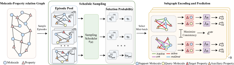
Figure 2: A 2-way 1-shot overview of GS-Meta. Firstly a Molecule-Property relation Graph (MPG) is constructed. Then, an episode candidate pool is randomly sampled, and the subgraph sampling scheduler $z_{(\phi)}$ is used to compute the selection probability $\eta$ and select a mini-batch containing $B$ episode pairs from the candidate pool. Finally, the relation learning module $f_{(\theta)}$ encodes each subgraph and outputs a classification loss $\mathcal{L}^{cls}$ within an episode and a contrastive loss $\mathcal{L}^{ctr}$ across episodes.

3 Graph Sampling-based Meta-Learning

This section presents the proposed Graph Sampling-based Meta-learning framework, as shown in Figure 2. We first define the few-shot molecular property prediction problem (Section 3.1). To establish and exploit the many-to-many relation between molecules and properties, we construct a Molecule-Property relation Graph (MPG) and then reformulate an episode in meta-learning as a subgraph from the MPG (Section 3.2). With this reformulation, we investigate to consider consistency and discrimination between subgraphs and schedule the subgraph sampling to facilitate meta-learning (Section 3.3). Finally, the training and testing strategies are described (Section 3.4).

3.1 Problem Definition

Following Altae-Tran et al. (2017); Guo et al. (2021), the few-shot molecular property prediction is conducted on a set of tasks $\left\{\mathcal{T}\right\}$, where each task $\mathcal{T}$ is to predict a property $p$ of molecules. The training set $\mathcal{D}_{train}$ consists of several tasks $\left\{\mathcal{T}_{train}\right\}$, denoted as $\mathcal{D}_{train}=\left\{(x_{i},y_{i,t})|t\in\mathcal{T}_{train}\right\}$, where $x_{i}$ is a molecule and $y_{i,t}$ is the label of $x_{i}$ on the $t$-th task. And the testing set $\mathcal{D}_{test}=\left\{(x_{j},y_{j,t})|t\in\mathcal{T}_{test}\right\}$ is composed of a set of tasks $\left\{\mathcal{T}_{test}\right\}$. $\{p_{train}\}$ and $\{p_{test}\}$ are denoted as properties corresponding to tasks $\{\mathcal{T}_{train}\}$ and $\{\mathcal{T}_{test}\}$, and training properties and testing properties are disjoint, i.e., $\{p_{train}\}\cap\{p_{test}\}=\emptyset$. The objective is to learn a predictor on $\mathcal{D}_{train}$ and to predict novel properties with a few labeled molecules in $\mathcal{D}_{test}$.

To deal with the few-shot problem, the episodic training paradigm has shown great promise in meta-learning Finn et al. (2017). Without loading all training tasks $\{\mathcal{T}_{train}\}$ into memory, batches of episodes $\{E_{t}\}_{t=1}^{B}$ are sampled iteratively in practical training process. To construct an episode $E_{t}$, a target task $\mathcal{T}_{t}$ is firstly sampled from $\left\{\mathcal{T}_{train}\right\}$, then a labeled support set $S_{t}$ and a query set $Q_{t}$ are sampled. Usually, there are two classes (i.e., active ($y$=1) or inactive ($y$=0)) in each molecular property prediction task, and a 2-way K-shot episode means that the support set $\mathcal{S}_{t}$ consists of 2 classes with K molecules per class, i.e., $\mathcal{S}_{t}=\left\{\left(x_{i}^{s},y_{i,t}^{s}\right)\right\}_{i=1}^{2K}$, and query set $\mathcal{Q}_{t}=\left\{\left(x_{i}^{q},y_{i,t}^{q}\right)\right\}_{i=1}^{M}$ contains $M$ molecules. In this case, we can define the episode as $E_{t}=(\mathcal{S}_{t},\mathcal{Q}_{t})$.

3.2 Molecule-Property Relation Graph

Graph Construction and Initialization

To leverage the rich information behind the relations among properties and molecules, we construct a Molecule-Property relation Graph (MPG) that explicitly describes such relations. The graph is denoted as $\mathcal{G}=(\mathcal{V},\mathcal{E})$, where $\mathcal{V}$ denotes the node set and $\mathcal{E}$ denotes the set of edges $e\in\mathcal{E}$. And there are two types of nodes in the graph, i.e., $\mathcal{V}=\mathcal{V}_{M}\cup\mathcal{V}_{T}$, where $\mathcal{V}_{M}=\left\{x_{m}\right\}$ is the molecule node set and $\mathcal{V}_{T}=\left\{p_{t}\right\}$ is the property node set. Edges $\mathcal{E}\subseteq\mathcal{V}_{M}\times\mathcal{V}_{T}$ are connected between these two types of nodes and the edge type of $e_{i,j}$ is initialized according to the label $y_{i,j}$, i.e., active (for $y$=1) or inactive (for $y$=0).

For a molecule $x_{i}$, a graph-based encoder Xu et al. (2019) is used following  Guo et al. (2021) to obtain its embedding:

$$\boldsymbol{x}_{i}=f_{mol}(x_{i}),$$ (1)

where $\boldsymbol{x}_{i}\in\mathbb{R}^{d}$. For a property node $p_{t}$, its embedding is randomly initialized for simplicity with the same length as molecules, i.e., $\boldsymbol{p}_{t}\in\mathbb{R}^{d}$. Hence the node features $\boldsymbol{h}_{i}^{0}$ are initialized with molecule and property embeddings respectively:

$$\boldsymbol{h}_{i}^{0}=\begin{cases}\boldsymbol{p}_{i}&\text{for }i\in\mathcal{V}_{T}\\ \boldsymbol{x}_{i}&\text{for }i\in\mathcal{V}_{M}\end{cases}.$$ (2)

Moreover, due to the deficiency of data, some molecules may not have labels on some auxiliary properties, leading to a missing edge connection between these molecules and properties. To make the graph topology compact, a special edge type unk is used to complement the missing label.

Reformulating Episode as Subgraph

The constructed MPG can be very large, e.g. in the PCBA dataset Wang et al. (2012), there are more than 430,000 molecules and 128 properties, and the corresponding MPG can contain more than 10 million edges. It is therefore computationally infeasible to directly work on the whole graph to predict molecular properties. Instead, we resort to subgraphs sampled from the MPG and connect them to episodes in meta-learning.

The episodic meta-learning, which is trained iteratively by sampling batches of episodes, has proven to be an effective training strategy Finn et al. (2017). Therefore, to adopt episodic meta-learning on MPG, we propose to reformulate the episode as a subgraph. Specifically, an episode of task $\mathcal{T}_{t}$ is equivalent to a subgraph containing a property node $p_{t}$ in $\mathcal{V}_{T}$, and molecules connected to $p_{t}$. Hence, the support set $\mathcal{S}_{t}$ can be reformulated as a subgraph of MPG:

$$\mathcal{S}_{t}\sim\mathcal{G}^{S}_{t}=\left\{\left(x_{i},e_{i,t},p_{t}\right),y_{i,t}|x_{i}\in\mathcal{N}(p_{t})\right\}_{i=1}^{2K},$$ (3)

where $p_{t}$ is a property node, and $\mathcal{N}(p_{t})$ is the neighbors of $p_{t}$. A query molecule is sampled as the query set, denoted as:

$$\mathcal{Q}_{t}\sim\mathcal{G}^{Q}_{t}=\{(x_{j},p_{t}),y_{j,t}|x_{j}\in\mathcal{N}(p_{t})\}.$$ (4)

By merging two subgraphs, the episode $E_{t}$ is reformulated as:

$$E_{t}\sim\mathcal{G}_{t}=\mathcal{G}^{S}_{t}\cup\mathcal{G}^{Q}_{t}.$$ (5)

The node and edge set of $\mathcal{G}_{t}$ are denoted as $\mathcal{V}^{t}$ and $\mathcal{E}^{t}$ respectively.

Since molecules have multiple properties, other available properties can be used when predicting a novel property of the same molecule. To leverage these auxiliary properties, we add some other property nodes connected to molecule nodes into the subgraph:

$$\mathcal{G}^{A}_{t}=\left\{\left(x_{i},e_{i,a},p_{a}\right),y_{i,a}|p_{a}\in\mathcal{N}(x_{i})\backslash p_{t}\right\}_{a=1}^{N_{a}},$$ (6)

where $N_{a}$ is the number of auxiliary property, $p_{a}$ is the auxiliary property node, $x_{i}\in\mathcal{V}^{t}_{M}$ is a molecule node in $\mathcal{G}_{t}$, and $\mathcal{G}_{t}^{A}$ is an auxiliary subgraph. With $\mathcal{G}_{t}^{A}$, we extend $\mathcal{G}_{t}$ as:

$$\mathcal{G}_{t}=\mathcal{G}_{t}\cup\mathcal{G}_{t}^{A}.$$ (7)

and there are totally $2K+N_{a}+2$ nodes, $2K$ support molecules, one query molecule, one target property, and $N_{a}$ auxiliary properties. From here on out, an episode of meta-learning and a subgraph of the MPG are semantically equivalent in this paper.

Subgraph Encoding and Prediction

We adopt a massage passing schema Hamilton et al. (2017) to iteratively update each sampled subgraph $\mathcal{G}_{t}$. In contrast to the previous work which only takes labels as edges Cao et al. (2021), we also consider relations between molecules, and design an edge predictor to estimate connections between molecules at each iteration:

$$\alpha_{i,j}^{l}=\sigma\left(\mathrm{MLP}\left(\exp\left(-|{\boldsymbol{h}_{i}^{l-1}}-\boldsymbol{h}_{j}^{l-1}|\right)\right)\right),$$ (8)

where $\sigma$ is Sigmoid function, $\boldsymbol{h}_{i}^{l-1}$ and $\boldsymbol{h}_{j}^{l-1}$ are embeddings of molecules $x_{i}$ and $x_{j}$ at ($l$-1)-th iteration respectively, and $\alpha_{i,j}^{l}$ is the estimated connection weight between $x_{i}$ and $x_{j}$. To avoid connecting dissimilar molecules, only top-k (k is hyper-parameter) edges with the largest estimated weights are kept and the edge type is mol2mol. Overall, there are four types of edges in $\mathcal{G}_{t}$, which are active, inactive and unk between a molecule and a property, and mol2mol between molecules.

After constructing the complete subgraph, node embeddings are updated as follows:

$$\boldsymbol{h}_{i}^{l}=\mathrm{GNN}^{l-1}\left(\boldsymbol{h}_{i}^{l-1},\boldsymbol{h}_{j}^{l-1},\boldsymbol{h}_{i,j}^{l-1},w_{i,j}^{l}|j\in\mathcal{N}\left(i\right)\right),$$ (9)

where $\boldsymbol{h}_{i}^{l}$ is the embedding of node $i$ at the l-th iteration, $\boldsymbol{h}_{i,j}^{l}$ is edge embedding initialized according to edge type, $\mathcal{N}(i)$ is neighbors of node $i$, and $w_{i,j}^{l}$ is the edge weight defined as:

$$w_{i,j}^{l}=\begin{cases}\alpha_{i,j}^{l}&e_{i,j}\in\mathcal{E}_{M,M}\\ 1&\text{otherwise}\end{cases},$$ (10)

where $\mathcal{E}_{M,M}$ is the set of edges between molecules. After $L$ iterations, the final embedding of molecule $\boldsymbol{h}_{i}^{L}$ and the property $\boldsymbol{h}_{t}^{L}$ are we concatenated to predict the label:

$$\hat{y}_{i,t}=\sigma\left(f_{cls}\left([\boldsymbol{h}_{i}^{L}\oplus\boldsymbol{h}_{t}^{L}]\right)\right),$$ (11)

where $\hat{y}_{i,t}\in\mathbb{R}^{1}$ is the prediction, and $\oplus$ is a concatenation operation. For simplicity, we denote $f_{(\theta)}$ as the relation learning module with parameter $\theta$, which includes molecular encoder $f_{mol}$, property initial embeddings, GNN layers, edge predictors, and classifier $f_{cls}$. More details are illustrated in Appendix A.3.

In each subgraph $\mathcal{G}_{t}$, the task classification loss on the support set $\mathcal{S}_{t}$ is calculated:

$$\mathcal{L}^{cls}_{t,\mathcal{S}}\left(f_{(\theta)}\right)=-\textstyle\sum_{\mathcal{S}_{t}}\left(y\log\hat{y}+\left(1-y\right)\log\left(1-\hat{y}\right)\right),$$ (12)

where $y$ and $\hat{y}$ are short for $y_{i,t}$ and $\hat{y}_{i,t}$ for clarity. Similarly, we can calculate the classification loss on the query set $\mathcal{L}^{cls}_{t,\mathcal{Q}}$.

3.3 Subgraph Sampling Scheduler

Previous few-shot molecular property prediction methods Guo et al. (2021); Wang et al. (2021) randomly sample episodes with a uniform probability, under the assumption that they are independent and of equal importance. However, subgraphs centered on different target properties are potentially connected to each other in the built MPG, due to the existence of intersecting nodes or edges. Hence, considering the subgraph dependency, we are motivated to develop a subgraph sampling scheduler that determines which episodes to use in the current batch during meta-training.

Consistency and Discrimination between Subgraphs

We specify the subgraph dependency in two aspects. (1) Each subgraph only has a small number of molecules ($K$ per class), and cannot contain all the information about the target property. For the same target property, subgraphs with different molecules (subgraph (i) and (ii) in Figure 1(b)) can be seen as different views describing the same task and they should be consistent with each other. (2) Meanwhile, subgraphs centered on different target property nodes (subgraph (ii) and (iii) in Figure 1(b)) are episodes of different tasks, and their semantic discrepancy should be enlarged.

Towards this end, the subgraph sampling scheduler, denoted as $z_{(\phi)}$ with parameters $\phi$, adopts a pairwise sampling strategy. That is, two subgraphs $\mathcal{G}_{t}^{(1)}$ and $\mathcal{G}_{t}^{(2)}$ of the same target property $p_{t}$ are sampled simultaneously. Specifically, at the beginning of each mini-batch, we randomly sample a pool of subgraph candidates, $\mathrm{P}=\{(\mathcal{G}_{t}^{(1)},\mathcal{G}_{t}^{(2)})\}_{t=1}^{N_{pool}}$, which are pairs of subgraphs for the same target property. For a subgraph $\mathcal{G}_{t}$, the scheduler $z_{(\phi)}$ outputs its selection probability $\eta_{t}$ via two steps. The first step calculates the subgraph embedding $\boldsymbol{g}_{t}$:

$$\boldsymbol{g}_{t}=\boldsymbol{h}_{t}^{L}+\sigma\left(\textstyle{\sum_{i\in\mathcal{V}^{t}\backslash p_{t}}\boldsymbol{h}_{i}^{L}}\right),$$ (13)

which is the pooling of the final embedding of each node, and $\boldsymbol{h}_{t}^{L}$ is final embedding of target property $p_{t}$. Then, we take $\boldsymbol{g}_{t}$ as input to the scheduler $z_{(\phi)}$ to get the selection probability $\eta_{t}$:

$$\eta_{t}=z_{1}\left(\boldsymbol{g}_{t}+z_{2}\left(\textstyle{\sum_{t^{\prime}\in\mathrm{P}\backslash\mathcal{G}_{t}}\boldsymbol{g}_{t^{\prime}}}\right)\right),$$ (14)

where $z_{1}$ and $z_{2}$ are MLP and together constitute $z_{(\phi)}$. Then, $\eta_{t}$ is normalized by softmax to get a reasonable probability value. Thus, for each episode pair $(\mathcal{G}_{t}^{(1)},\mathcal{G}_{t}^{(2)})$ in the candidate pool, the selection probability can be computed as $(\eta_{t}^{(1)}+\eta_{t}^{(2)})/2$, and we sample $B$ from $N_{pool}$ in the candidate pool to form a mini-batch according to selection probability.

To encourage consistency between subgraphs of the same target property and discrimination between different target properties, we adopt the NT-Xent loss Hjelm et al. (2019) which is widely used in contrastive learning. Subgraphs of the same target property are positive pairs and those of different target properties are negatives, and the contrastive loss in a mini-batch is as follows:

$$\mathcal{L}^{ctr}=\frac{1}{B}\sum_{t=1}^{B}-\log\frac{e^{\mathrm{sim}\left(\boldsymbol{g}_{t}^{(1)},\boldsymbol{g}_{t}^{(2)}\right)/\tau}}{\sum_{t^{\prime}=1,t^{\prime}\neq t}^{B}e^{\mathrm{sim}\left(\boldsymbol{g}_{t}^{(1)},\boldsymbol{g}_{t^{\prime}}^{(2)}\right)/\tau}},$$ (15)

where $B$ is mini-batch size, $\mathrm{sim}(\cdot,\cdot)$ is cosine similarity and $\tau$ is the temperature parameter.

Algorithm 1 Training and optimization algorithm.

Input: Molecule-Property relation Graph (MPG)
Output: Relation learning module $f_{(\theta)}$, subgraph sampling scheduler $z_{(\phi)}$.

1:  while not done do

2:     Sample $N_{pool}$ episode pairs $\{(\mathcal{G}_{t}^{(1)},\mathcal{G}_{t}^{(2)})\}_{t=1}^{N_{pool}}$ as candidates

3:     Calculate selection probability $\eta_{t}$ by Eqn. (14) for each candidate episode

4:     Select $B$ episode pairs $\{(\mathcal{G}_{t}^{(1)},\mathcal{G}_{t}^{(2)})\}_{t=1}^{B}$ from candidates according to $\eta_{t}$ to form a mini-batch

5:     for $t=1,\dots,B$ do

6:        Calculate classification loss on support set $\mathcal{L}^{cls}_{t,\mathcal{S}}$ by Eqn. (12) on both $\mathcal{G}_{t}^{(1)}$ and $\mathcal{G}_{t}^{(2)}$

7:        Do inner-loop update $\theta^{\prime}\leftarrow\theta-\beta_{inner}\nabla_{\theta}\mathcal{L}_{t,\mathcal{S}}^{cls}\left(f_{(\theta)}\right)$ on both $\mathcal{G}_{t}^{(1)}$ and $\mathcal{G}_{t}^{(2)}$

8:        Calculate classification loss on query set $\mathcal{L}^{cls}_{t,\mathcal{Q}}$ by Eqn. (12) on both $\mathcal{G}_{t}^{(1)}$ and $\mathcal{G}_{t}^{(2)}$

9:     end for

10:     Calculate contrastive loss $\mathcal{L}^{ctr}$ by Eqn. (15)

11:     Do outer-loop optimization by Eqn. (17)

12:     Update scheduler $z$ by Eqn. (19)

13:  end while

3.4 Training and Testing

In this subsection, we introduce the optimization strategy of relation learning module $f_{(\theta)}$ and subgraph sampling scheduler $z_{(\phi)}$ in training and testing.

Optimization of Relation Learning Module

Following Finn et al. (2017), a gradient descent strategy is adopted to obtain a good initialization. Firstly, at the beginning of a mini-batch, subgraph sampling scheduler $z$ is used to sample B episode pairs $\{(\mathcal{G}_{t}^{(1)},\mathcal{G}_{t}^{(2)})\}_{t=1}^{B}$ from candidates.

For each episode, in the inner-loop optimization, the loss on the support set defined in Eqn.(12) is computed to update the parameters $\theta$ by gradient descent:

$$\theta^{\prime}\leftarrow\theta-\beta_{inner}\nabla_{\theta}\mathcal{L}_{t,\mathcal{S}}^{cls}\left(f_{(\theta)}\right),$$ (16)

where $\beta_{inner}$ is the learning rate. After updating the parameter, the loss of query set is computed, denoted as ${{\mathcal{L}_{t,\mathcal{Q}}^{cls}}}$. Finally, we do an outer loop to optimize both the classification and contrastive loss with learning rate $\beta_{outer}$ across the mini-batch:

$$\theta\leftarrow\theta-\beta_{outer}\nabla_{\theta}\mathcal{L}\left(f_{(\theta^{\prime})}\right),$$ (17)

where the meta-training loss $\mathcal{L}\left(f_{(\theta^{\prime})}\right)$ is computed across the mini-batch:

$$\mathcal{L}\left(f_{(\theta^{\prime})}\right)=\frac{1}{2B}\sum_{t=1}^{B}\left({{\mathcal{L}_{t,\mathcal{Q}}^{cls}}}^{(1)}+{{\mathcal{L}_{t,\mathcal{Q}}^{cls}}}^{(2)}\right)+\lambda\mathcal{L}^{ctr},$$ (18)

where $\lambda$ is hyperparameter and $\mathcal{L}^{ctr}$ is defined by Eqn.(15), and ${{\mathcal{L}_{t,\mathcal{Q}}^{cls}}}^{(1)}$, ${{\mathcal{L}_{t,\mathcal{Q}}^{cls}}}^{(2)}$ are query loss of $\mathcal{G}_{t}^{(1)}$ and $\mathcal{G}_{t}^{(2)}$ respectively. The complete procedure is described in Algorithm 1.

In testing, for a new property $p_{t}$ in $\{p_{test}\}$, auxiliary properties are selected from $\{p_{train}\}$ and $f_{(\theta)}$ is finetuned by Eqn.(16).

Optimization of Subgraph Sampling Scheduler

Since sampling cannot be directly differentiated, similar to Yao et al. (2021), we use policy gradient Williams (1992) to optimize the scheduler $z_{(\phi)}$. To encourage mining negative samples that are indistinguishable from positives, it is intuitive to take the value of contrastive loss $\mathcal{L}^{ctr}$ as reward $R$:

$$\phi\leftarrow\phi+\gamma\nabla_{\phi}\log P\left(\boldsymbol{\eta}\right)\left({R}-b\right),$$ (19)

where $\boldsymbol{\eta}=\{\eta_{t}\}_{t=1}^{B}$ is selection probability of sampled episode in a mini-batch, $\gamma$ is learning rate and $b$ is moving average of reward.

4 Experiments

The following research questions guide the remainder of the paper. (RQ1) Can our proposed GS-Meta outperform SOTA baselines? (RQ2) How do auxiliary properties affect the performance? (RQ3) Can the episode reformulation and sampling scheduler improve performance? (RQ4) How to interpret the scheduler that models the episode relationship?

4.1 Experimental Setup

We use five common few-shot molecular property prediction datasets from the MoleculeNet Wu et al. (2018). Details are in Appendix B.

For a comprehensive comparison, we adopt two types of baselines: (1) methods with molecular encoder learned from scratch, including Siamese Koch et al. (2015), ProtoNet Snell et al. (2017), MAML Finn et al. (2017), TPN Liu et al. (2019), EGNN Kim et al. (2019), IterRefLSTM Altae-Tran et al. (2017), and PAR Wang et al. (2021); and (2) methods which leverage pre-trained molecular encoder, including Pre-GNN Hu et al. (2020), Meta-MGNN Guo et al. (2021), Pre-PAR Wang et al. (2021) and we denote Pre-GS-Meta as our method equipped with Pre-GNN. More details about these baselines are in Appendix C.1. We run experiments 10 times with different random seeds and report the mean and standard deviations.

Method	Tox21		SIDER		MUV		ToxCast		PCBA
	10-shot	1-shot	10-shot	1-shot	10-shot	1-shot	10-shot	1-shot	10-shot	1-shot
Siamese	$80.40_{(0.35)}$	$65.00_{(1.58)}$	$71.10_{(4.32)}$	$51.43_{(3.31)}$	$59.96_{(5.13)}$	$50.00_{(0.17)}$	-	-	-	-
ProtoNet	$74.98_{(0.32)}$	$65.58_{(1.72)}$	$64.54_{(0.89)}$	$57.50_{(2.34)}$	$65.88_{(4.11)}$	$58.31_{(3.18)}$	$68.87_{(0.43)}$	$58.55_{(0.52)}$	$64.93_{(1.94)}$	$55.79_{(1.45)}$
MAML	$80.21_{(0.24)}$	$75.74_{(0.48)}$	$70.43_{(0.76)}$	$67.81_{(1.12)}$	$63.90_{(2.28)}$	$60.51_{(3.12)}$	$68.30_{(0.59)}$	$61.12_{(0.94)}$	$66.22_{(1.31)}$	$62.04_{(1.73)}$
TPN	$76.05_{(0.24)}$	$60.16_{(1.18)}$	$67.84_{(0.95)}$	$62.90_{(1.38)}$	$65.22_{(5.82)}$	$50.00_{(0.51)}$	-	-	-	-
EGNN	$81.21_{(0.16)}$	$79.44_{(0.22)}$	$72.87_{(0.73)}$	$70.79_{(0.95)}$	$65.20_{(2.08)}$	$62.18_{(1.76)}$	$74.02_{(1.11)}$	$64.17_{(0.89)}$	$69.92_{(1.85)}$	$62.14_{(1.58)}$
IterRefLSTM	$81.10_{(0.17)}$	$\underline{80.97}_{(0.10)}$	$69.63_{(0.31)}$	$71.73_{(0.14)}$	$49.56_{(5.12)}$	$48.54_{(3.12)}$	-	-	-	-
PAR	$\underline{82.06}_{(0.12)}$	$80.46_{(0.13)}$	$\underline{74.68}_{(0.31)}$	$\underline{71.87}_{(0.48)}$	$\underline{66.48}_{(2.12)}$	$\underline{64.12}_{(1.18)}$	$\underline{74.78}_{(1.53)}$	$\underline{69.45}_{(1.24)}$	$\underline{70.05}_{(0.94)}$	$\underline{67.77}_{(1.04)}$
GS-Meta	$\textbf{85.85}_{(0.26)}$	$\textbf{84.32}_{(0.89)}$	$\textbf{83.72}_{(0.54)}$	$\textbf{82.84}_{(0.67)}$	$\textbf{67.11}_{(1.95)}$	$\textbf{64.70}_{(2.88)}$	$\textbf{81.55}_{(0.19)}$	$\textbf{80.03}_{(0.26)}$	$\textbf{72.16}_{(0.71)}$	$\textbf{70.03}_{(1.56)}$
Pre-GNN	$82.14_{(0.08)}$	$81.68_{(0.09)}$	$73.96_{(0.08)}$	$73.24_{(0.12)}$	$67.14_{(1.58)}$	$64.51_{(1.45)}$	-	-	-	-
Meta-MGNN	$82.97_{(0.10)}$	$82.13_{(0.13)}$	$75.43_{(0.21)}$	$73.36_{(0.32)}$	$68.99_{(1.84)}$	$65.54_{(2.13)}$	-	-	-	-
Pre-PAR	$\underline{84.93}_{(0.11)}$	$\underline{83.01}_{(0.09)}$	$\underline{78.08}_{(0.16)}$	$\underline{74.46}_{(0.29)}$	$\underline{69.96}_{(1.37)}$	$\underline{66.94}_{(1.12)}$	$\underline{79.41}_{(0.08)}$	$\underline{76.58}_{(0.15)}$	$\underline{73.71}_{(0.61)}$	$\underline{72.49}_{(0.61)}$
Pre-GS-Meta	$\textbf{86.91}_{(0.41)}$	$\textbf{86.46}_{(0.55)}$	$\textbf{85.08}_{(0.54)}$	$\textbf{84.45}_{(0.26)}$	$\textbf{70.18}_{(1.25)}$	$\textbf{67.15}_{(2.04)}$	$\textbf{83.81}_{(0.16)}$	$\textbf{81.57}_{(0.18)}$	$\textbf{79.40}_{(0.43)}$	$\textbf{78.16}_{(0.47)}$

Table 1: ROC-AUC scores on benchmark datasets, compared with methods learned from scratch (first group) and methods that leverage pre-trained molecular encoder (second group). The best is marked with boldface and the second best is with underline.

4.2 Main Results (RQ1)

The overall performance is shown in Table 1. The experimental results show that our GS-Meta and Pre-GS-Meta outperform all baselines consistently with 6.93% and 5.71% average relative improvement respectively. Moreover, those relation-graph-based methods (i.e., TPN, EGNN, PAR and GS-Meta) mostly perform better than traditional methods. This indicates that it is effective to exploit relations between molecules in a graph and it is more effective to exploit both molecules and properties together as our method performs best. Further, the improvement varies across different datasets. For example, GS-Meta gains 13.68% improvement on SIDER but 0.93% improvement on MUV. We argue this is due to the fact that there are more auxiliary properties available on SIDER, and also that there are no missing labels in SIDER compared to 84.2% missing labels on MUV. Fewer auxiliary properties and the presence of missing labels prevent utilizing information from auxiliary properties. This phenomenon is further investigated in Section 4.3.

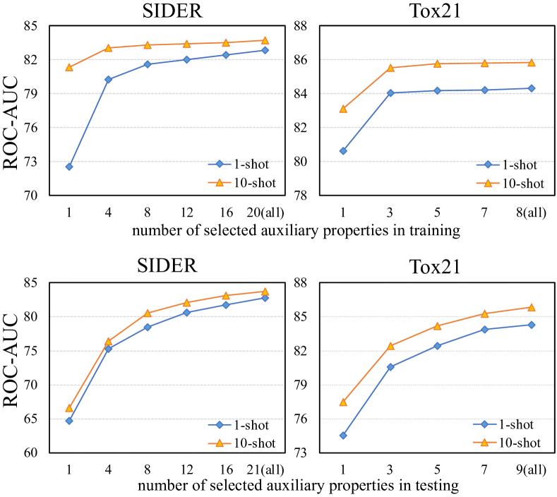
Figure 3: Performance of different numbers of selected auxiliary properties in training (top) and testing (bottom).

4.3 Analysis of Auxiliary Property (RQ2)

Effect of the Number of Auxiliary Properties

We explore the effect of auxiliary properties by varying the number of sampled auxiliary properties. Since auxiliary property sampling occurs during both training and testing, here we consider two scenarios: 1) effect of the number of sampled auxiliary properties during training: keep the number of sampled auxiliary properties during testing constant and change the number during training; 2) effect of the number of sampled auxiliary properties during testing: keep the number of sampled auxiliary properties during training constant and change the number during testing.

As shown in Figure 3, the performance improves as the number of auxiliary properties increases in both training and testing, confirming our motivation that known properties of molecules help predict new properties. This is because more auxiliary properties contain more information at each training and inference step. In addition, reducing the number of auxiliary properties in training has less impact on performance than in testing, which suggests that when faced with a large number of auxiliary properties, sampling some of them during training can be an effective way to train the model and does not lead to significant performance degradation.

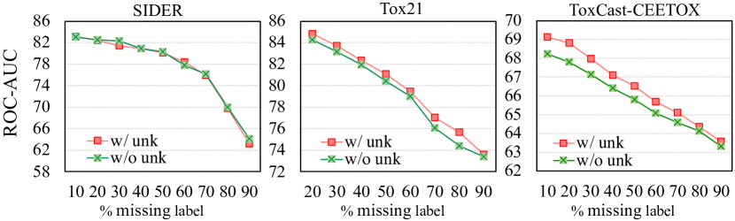
Figure 4: Performance with different missing label ratios in SIDER, Tox21 and ToxCast-CEETOX under the 10-shot scenario.

Effect of the Ratio of Missing Labels

We further investigate the effect of missing labels on auxiliary properties by randomly masking labels in the training set, which means the model has less training data and fewer auxiliary properties possible for testing. Two different approaches are compared: 1) w/ unk: completing missing label with a special edge unk; 2) w/o unk: no process of the missing label.

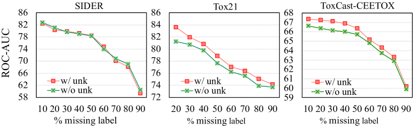
Figure 6: Performance with different missing label ratios in SIDER, Tox21 and ToxCast-CEETOX under the 1-shot scenario.

Figure 4 shows the results under the 10-shot scenario. Since the proportion of missing labels in the training set on Tox21 itself is higher than 10%, we start masking from 20%. The performance gradually decreases as the percentage of missing labels increases. In addition, unk edges have no noticeable effect on SIDER, but improve performance on Tox21 and ToxCast-CEETOX by 0.81% and 0.96% respectively. This can be due to imbalanced labeling: SIDER is more balanced than Tox21 and ToxCast-CEETOX. Moreover, the results show that when masking 70%, 40% and 40% training labels on SIDER, Tox21 and ToxCast-CEETOX respectively, our method still achieves a comparable performance against SOTA. It proves that our method has robust and promising performance despite the missing training data. Results under the 1-shot scenario is in Figure 6 in Appendix.

4.4 Analysis of Episode Reformulation and Sampling Scheduler (RQ3)

Ablation Study

We conduct ablations to study the effectiveness of episode reformulation and sampling scheduler. For episode reformulation, the following variants are analyzed: 1)w/o m2m: remove mol2mol edges in MPG; 2)w/o E: remove edge type in MPG, i.e., do message passing in Eqn.(9) without $\boldsymbol{h}_{i,j}$. For the sampling scheduler, the following variants are analyzed: 1)w/o S: randomly select episode without a sampling scheduler; 2)w/o CL: optimize model parameters in Eqn. (17) without contrastive loss $\mathcal{L}^{ctr}$; 3)w/o S, w/o CL: do not use scheduler and contrastive loss.

As in Table 2, GS-Meta outperforms all the variants, indicating that our proposed subgraph reformulation and scheduling strategy are effective. Results on SIDER are in Table 10 in Appendix. Removing the type of edges causes a significant performance drop, which validates that the information of labels can be fused into the graph by using them as edge types. And removing both contrastive loss and the scheduler degrades the model performance, indicating that our design of contrastive loss and the scheduler is reasonably effective.

Method	1-shot	10-shot
GS-Meta	84.32	85.85
w/o m2m	83.91($\downarrow$0.41)	84.80($\downarrow$1.05)
w/o E	72.54($\downarrow$11.78)	75.93($\downarrow$9.92)
w/o S	83.14($\downarrow$1.18)	84.51($\downarrow$1.34)
w/o CL	83.30($\downarrow$1.02)	84.66($\downarrow$1.19)
w/o S, w/o CL	82.64($\downarrow$1.68)	84.32($\downarrow$1.53)

Table 2: Ablation study on Tox21

Method	1-shot	10-shot
PAR	70.41(0.83s)	74.65(1.13s)
PAR (w/ ATS)	69.94(2.42s)	75.10(2.90s)
GS-Meta	85.94(3.11s)	87.67(3.59s)
GS-Meta (w/ ATS)	84.73(6.80s)	86.88(7.11s)
GS-Meta (w/o S)	84.72(2.20s)	86.81(2.60s)

Table 3: Performance and time cost on ToxCast-BSK

Comparing with Other Scheduler

To further explore the effects of the designed sampling scheduler, we compare PAR and our GS-Meta with other scheduler. Here we adopt ATS Yao et al. (2021), which is a SOTA task scheduler for meta-learning proposed recently. ATS takes gradient and loss as input to characterize the difficulty of candidate tasks. For a comprehensive evaluation, we compare both the performance and time cost of a mini-batch during training.

The results on ToxCast-BSK are in Table 3, where (w/ ATS) indicates using ATS as the sampling scheduler and (w/o S) indicates randomly selecting without the scheduler. Note that the original PAR itself does not have a scheduler. We reach two conclusions. First, ATS does not improve performance significantly (PAR(w/ ATS) vs PAR, GS-Meta(w/ ATS) vs GS-Meta(w/o S)). This suggests that ATS is not applicable in our scenario of few-shot molecular property prediction and the SOTA methods. And our scheduler is able to improve the model performance (GS-Meta vs GS-Meta(w/o S)). Secondly, ATS is more time-consuming. ATS is around three times slower compared with random sampling (PAR(w/ ATS) vs PAR, GS-Meta(w/ ATS) vs GS-Meta(w/o S)), but our scheduler is faster (GS-Meta vs GS-Meta(w/o S)). This is because ATS needs to compute the loss and gradient backpropagation for each candidate and sample a validation set to get the reward for optimization. While our approach is to reformulate an episode as a subgraph and get the representation of episode by directly encoding it. And we use a contrastive loss to uniformly model the relationship between episodes and as an optimization reward for the scheduler. Results on ToxCast-APR are in Table 11 in Appendix.

4.5 Interpretation of the Scheduler (RQ4)

To understand the sampling scheduler, we visualize the sampling result of 9 properties in the training set on Tox21 in Figure 5. The cosine similarity of property embeddings on Tox21 is also visualized. In the sampling result heatmap, the value in row i column j indicates the number of times that property i and property j are sampled in the same mini-batch at the same time. And we run the scheduler 200 times to statistically count the results.

We observe that more similar properties are sampled into the same mini-batch more frequently, e.g., property SR-ATAD5 with property NR-AR and property NR-ER with property NR-PPAR-gamma. And dissimilar properties are sampled less frequently in one mini-batch, e.g., property NR-ER-LBD with property NR-AR-LBD and property SR-ATAD5 with property NR-ER-LBD. This indicates that our scheduler prefers to put similar properties in one mini-batch, analogous to mining hard negative samples. Nevertheless, the sampling result is not exactly consistent with the property embedding similarity, because the scheduler’s input is the final pooled embedding of the subgraph, not only the embedding of the target property.

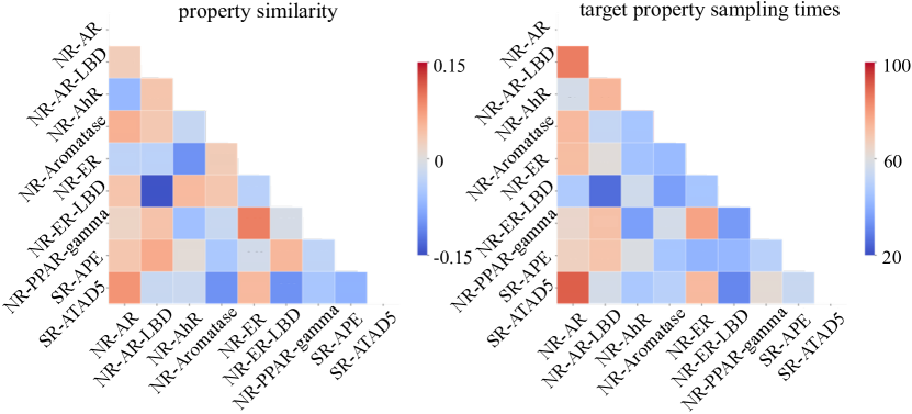
Figure 5: Heatmap of property similarity and statistics of target property sampling times on Tox21.

5 Conclusion

We propose a Graph Sampling-based Meta-learning framework to effectively leverage other available properties to predict new properties with a few labeled samples in molecular property prediction. Specifically, we construct a Molecule-Property relation Graph and reformulate an episode in meta-learning as a subgraph of MPG. Further, we consider subgraph consistency and discrimination and schedule the subgraph sampling via a contrastive loss. Empirical results show GS-Meta outperforms previous methods consistently.

This work only considers 2-way classification tasks and does not involve regression tasks. This is because the commonly-used benchmarks for few-shot molecular property prediction are 2-way tasks and few are eligible regression datasets. Our method can generalize to multi-class and regression cases, by assigning different edge attribute values. We put this in future works.

Appendix

Appendix A Details of GS-Meta

A.1 Notations

For ease of understanding, we summarize notations and descriptions in Table 5.

A.2 Reasons to Sampling Subgraphs as Episodes

The size of the constructed MPG can be very large (e.g., containing more than 400,000 molecules in PCBA dataset), and it is not possible to compute direcly on the whole graph during training. Because the molecular encoder $f_{mol}$ needs to encode each molecule to get the initial embedding of molecular nodes in the graph. Encoding molecules using molecular encoder and encoding MPG using GNN, and then doing gradient back propagation will lead to an Out-of-Memory error.

A.3 GNN Layer

Eqn. (9) follows a message passing paradigm, in which embedding is updated by aggregating the information passed from neighboring nodes and edges. At $l$-th iteration, firstly the aggregated neighborhood embedding $\boldsymbol{h}_{\mathcal{N}_{(i)}}^{l}$ is obtained:

$$\boldsymbol{h}^{l}_{\mathcal{N}_{(i)}}\leftarrow\frac{1}{|\mathcal{N}_{(i)}|}\sum_{j\in\mathcal{N}_{(i)}}\left(\left(\boldsymbol{h}_{j}^{l-1}+\boldsymbol{h}_{i,j}^{l-1}\right)\times w_{i,j}^{l}\right)$$ (20)

where $\mathcal{N}_{(i)}$ is neighbors of node $i$, $\boldsymbol{h}_{i,j}^{l-1}$ and $w_{i,j}^{l}$ is embedding and weight of edge. And then we do combination to process information received from neighborhood and node’s previous layer embedding $\boldsymbol{h}_{i}^{l-1}$:

$$\boldsymbol{h}^{l}_{i}\leftarrow\mathrm{LeakyReLU}\left(\mathbf{W}^{(l)}_{\mathrm{msg}}\boldsymbol{h}^{l}_{\mathcal{N}_{(i)}}+\mathbf{W}^{(l)}_{\mathrm{root}}\boldsymbol{h}_{i}^{l-1}\right),$$ (21)

where $\mathbf{W}^{(l)}_{\mathrm{msg}}$ and $\mathbf{W}^{(l)}_{\mathrm{root}}$ are trainable parameters included in parameters $\theta$ of relation learning module $f_{(\theta)}$.

Dataset	Tox21	SIDER	MUV	ToxCast	PCBA
#Compound	7831	1427	93127	8575	437929
#Property	12	27	17	617	128
#Train Property	9	21	12	451	118
#Test Property	3	6	5	158	10
%Label active	6.24	56.76	0.31	12.60	0.84
%Label inactive	76.71	43.24	15.76	72.43	59.84
%Missing Label	17.05	0	84.21	14.97	39.32

Table 4: Dataset statistics

Appendix B Details of Datasets

B.1 Datasets Description

We conduct experiments on five widely used few-shot molecular property prediction datasets(Table 4) in MoleculeNet benchmark Wu et al. [2018]:

• Tox21 is a public database on compound toxicity, which has been used in the 2014 Tox21 Data Challenge.

• SIDER Kuhn et al. [2016] contains marketed drugs and adverse drug reactions(ADR), which are grouped into 27 system organ classes.

• MUV Rohrer and Baumann [2009] is selected by applying a redefined nearest neighbor analysis for validation of virtual screening techniques.

• ToxCast Richard et al. [2016] provides toxicology data for a large quantities of compounds based on in vitro high-throughput screening.

• PCBA Wang et al. [2012] consists of small molecule bioactivities generated by high-throughput screening.

Table 5: Notations and Description

Notation	Description
$\mathcal{D}_{test}$	Training data set
$\mathcal{D}_{test}$	Testing data set
$\{\mathcal{T}_{train}\}$	Training task set
$\{\mathcal{T}_{test}\}$	Testing task set
$\mathcal{S}_{t},\mathcal{Q}_{t}$	Support and query set of task $\mathcal{T}_{t}$
$E_{t}$	One episode of task $\mathcal{T}_{t}$
$\mathcal{G}$	Sample-Property relation Graph
$\mathcal{V}$,$\mathcal{E}$	Node and edge set of $\mathcal{G}$
$\mathcal{V}_{T}$	Property node set
$\mathcal{V}_{M}$	Molecule node set
$p_{t}$	The $t$-th property node in $\mathcal{G}$
$x_{i}$	The $i$-th molecule node in $\mathcal{G}$
$\{p_{train}\}$	property nodes corresponding to $\{\mathcal{T}_{train}\}$
$\{p_{test}\}$	property nodes corresponding to $\{\mathcal{T}_{test}\}$
$\boldsymbol{p_{t}}$	Initial embedding of $t$th property node
$\boldsymbol{x_{i}}$	Initial embedding of $i$th molecule node
$e_{i,j}$	Edge between node $i$ and node $j$
$\mathcal{G}_{S}^{t}$	Subgraph in $\mathcal{G}$ analogous to $\mathcal{S}_{t}$
$\mathcal{G}_{Q}^{t}$	Subgraph in $\mathcal{G}$ analogous to $\mathcal{Q}_{t}$
$\mathcal{G}_{A}^{t}$	Auxiliary subgraph in $\mathcal{G}$
$\mathcal{G}_{t}$	Subgraph in $\mathcal{G}$ analogous to $E_{t}$
$\boldsymbol{h}_{i}^{l}$	Embedding of node $i$ at $l$-th layer
$\boldsymbol{h}_{i,j}^{l}$	Embedding of edge $(i,j)$ at $l$-th layer
$\alpha_{i,j}^{l}$	Estimated weight of molecule edge $(i,j)$ at $l$-th layer
$w_{i,j}^{l}$	Edge weight of $(i,j)$ at $l$-th layer
$\hat{y}_{i,t}$	Predicted label of molecule $i$ on property $t$
$f_{(\theta)}$	relation learning module with parameter $\theta$
$z_{(\phi)}$	the sampling scheduler with parameter $\phi$
$\boldsymbol{g}_{t}$	subgraph embedding of $\mathcal{G}_{t}$
$\eta_{t}$	selection propability
$\mathcal{L}^{ctr}$	Contrastive loss in a minibatch
${\mathcal{L}_{t,\mathcal{Q}}^{cls}}$	Classification loss of query set on episode $\mathcal{G}_{t}$
${\mathcal{L}_{t,\mathcal{S}}^{cls}}$	Classification loss of support set on episode $\mathcal{G}_{t}$

Assay Provider	#Compound	#Property	#Train Property	#Test Property	%Label active	%Label inactive	%Missing Label
APR	1039	43	33	10	10.30	61.61	28.09
ATG	3423	146	106	40	5.92	93.92	0.16
BSK	1445	115	84	31	17.71	82.29	0
CEETOX	508	14	10	4	22.26	76.38	1.36
CLD	305	19	14	5	30.72	68.30	0.98
NVS	2130	139	100	39	3.21	4.52	92.27
OT	1782	15	11	4	9.78	87.78	2.44
TOX21	8241	100	80	20	5.39	86.26	8.35
Tanguay	1039	18	13	5	8.05	90.84	1.11

Table 6: Details of sub-datasets of ToxCast.

hyper-parameter	Description	Range	Selected
$d$	dimension of molecule and property embedding.	300	300
$L$	number of GNN layer.	1$\sim$3	2
$\beta_{inner}$	learning rate in inner-loop.	0.01$\sim$0.5	0.05
$\beta_{outer}$	learning rate in outer-loop.	0.001	0.001
$\gamma$	learning rate of subgraph sampling scheduler.	0.0001$\sim$0.001	0.0005
$\tau$	temperature in Eqn. (15) .	0.05$\sim$0.5	0.08
$\lambda$	regularization of contrastive loss in Eqn. (15).	0.01$\sim$0.5	0.05

Table 7: The hyper-parameters.

Method	APR	ATG	BSK	CEETOX	CLD	NVS	OT	TOX21	Tanguay
MAML	$64.59$	$55.45$	$60.36$	$61.02$	$66.22$	$59.84$	$62.15$	$59.52$	$60.92$
ProtoNet	$57.08$	$54.92$	$53.92$	$60.25$	$66.25$	$54.87$	$63.11$	$58.27$	$58.32$
EGNN	$67.06$	$57.28$	$60.82$	$60.10$	$71.53$	$56.56$	$66.08$	$63.32$	$74.80$
PAR	$\underline{74.24}$	$\underline{63.48}$	$\underline{70.41}$	$\underline{61.44}$	$\underline{75.76}$	$\underline{67.56}$	$\underline{65.72}$	$\underline{68.94}$	$\underline{77.54}$
GS-Meta	87.90	79.62	85.94	67.49	78.16	71.04	72.36	87.84	89.97
Pre-PAR	$\underline{84.69}$	$\underline{70.38}$	$\underline{79.89}$	$\underline{66.57}$	$\underline{77.83}$	$\underline{72.51}$	$\underline{70.41}$	$\underline{80.33}$	$\underline{86.64}$
Pre-GS-Meta	89.49	81.69	87.28	68.55	78.69	74.36	73.56	89.46	91.10

Table 8: Detailed performance on each sub-dataset of ToxCast in 1-shot scenario.

Method	APR	ATG	BSK	CEETOX	CLD	NVS	OT	TOX21	Tanguay
MAML	$72.66$	$62.09$	$66.42$	$64.08$	$74.57$	$66.56$	$64.07$	$68.04$	$77.12$
ProtoNet	$73.58$	$59.26$	$70.15$	$66.12$	$78.12$	$65.85$	$64.90$	$68.26$	$73.61$
EGNN	$80.33$	$66.17$	$73.43$	$66.51$	$\underline{78.85}$	$\underline{71.05}$	$68.21$	$76.40$	$\underline{85.23}$
PAR	$\underline{82.74}$	$\underline{68.86}$	$\underline{74.65}$	$\underline{67.76}$	$78.33$	$70.79$	$\underline{69.12}$	$\underline{77.34}$	$83.39$
GS-Meta	88.95	80.44	87.67	69.50	79.95	74.77	73.46	88.78	90.48
Pre-PAR	$\underline{86.09}$	$\underline{72.72}$	$\underline{82.45}$	$\underline{72.12}$	$\underline{83.43}$	$\underline{74.94}$	$\underline{71.96}$	$\underline{82.81}$	$\underline{88.20}$
Pre-GS-Meta	90.15	82.54	88.21	74.19	86.34	76.29	74.47	90.63	91.47

Table 9: Detailed performance on each sub-dataset of ToxCast in 10-shot scenario.

B.2 Datasets Splitting

We adopt public splits provided by  Altae-Tran et al. [2017] on Tox21, SIDER and MUV. For PCBA, we choose the first 5 and last 5 properties as meta-testing and the rest of properties as meta-training. For ToxCast, since the dataset is sparse overall, but the properties can be grouped according to assay providers, and the grouping gives denser results. We first group the dataset by assay providers to obtain a number of sub-datasets, and after discarding sub-datasets with few properties, each sub-dataset is divided into meta-training and meta-testing and the average of the performance of all sub-datasets is finnaly reported. Details of each sub-dataset are shown in Table 6 and detailed results of each sub-dataset are in Table 8 and Table 9.

Appendix C Details of Implementation

All experiments are conducted on a Ubuntu Server with one 32 GB NVIDIA Tesla V100 GPU.

C.1 Baselines

We adopt two types of baselines, and details of each are listed as follows:
Learn from Scratch: FSL methods with a random initialized molecular encoder.

• Siamese Koch et al. [2015] uses a duel network to determine if inputs are of the same class.

• ProtoNet Snell et al. [2017] classifies inputs based on distance between class prototypes.

• MAML Finn et al. [2017] learns a good model parameter initialization and adapts fast on new tasks via optimization.

• TPN Liu et al. [2019] constructs a relation graph from input samples via similarity of input and makes label propagation.

• EGNN Kim et al. [2019] constructs a relation graph from input samples via similarity of input and predicts labels by edges in a graph.

• IterRefLSTM Altae-Tran et al. [2017] adopts a variant of MatchingNet Vinyals et al. [2016] in molecular property prediction.

• PAR Wang et al. [2021] leverages class prototypes to update input representations and designs label propagation for similar inputs in relation graph.

Leverage Pre-trained Model: methods which leverage a pretrained molecular encoder Hu et al. [2020].

• Pre-GNN Hu et al. [2020] is a pretrained GNN model using self-supervised tasks and is directly finetuned on the support set.

• Meta-MGNN Guo et al. [2021] uses Pre-GNN and add self-supervised tasks in meta-training.

• Pre-PAR Wang et al. [2021] is PAR initialized with Pre-GNN.

For Tox21, SIDER and MUV, results reported in Wang et al. [2021] are used. For ToxCast we resplit it and implement baselines using public codes on ToxCast and PCBA.

C.2 GS-Meta

We implement GS-Meta in Pytorch Paszke et al. [2019] and Pytorch Geometric library Fey and Lenssen [2019]. For a fair comparison we adopt a 5-layer GIN Xu et al. [2019] as molecular encoder for GS-Meta and all baselines. The maximum number of optimization step in meta-training is 2000 and meta-testing is evaluated every 100 steps. MLP in Eqn. (8) and $f_{cls}$ in Eqn. (11) consist two fully connected layers with hidden size 128. Number of candidates $N_{pool}$ and batch size $B$ is 10 and 5 respectively. Hyper-parameter k of connecting molecules is set to 1 in 1-shot and 9 in 10-shot scenario. Table 7 illustrates all the hyper-parameters and the results of hyper-parameter sensitivity analysis are in Table 12. For the number of selected auxiliary properties, on Tox21, SIDER and MUV, we select all possible auxiliary properties in training and testing. On ToxCast and PCBA, the maximum number is 20 in both training and testing.

Method	1-shot	10-shot
GS-Meta	82.84	83.72
w/o m2m	82.12($\downarrow$0.72)	83.09($\downarrow$0.63)
w/o E	57.54($\downarrow$25.30)	61.85($\downarrow$21.87)
w/o S	81.07($\downarrow$1.78)	82.23($\downarrow$1.49)
w/o CL	81.36($\downarrow$1.48)	82.52($\downarrow$1.20)
w/o S, w/o CL	80.69($\downarrow$2.15)	81.94($\downarrow$1.78)

Table 10: Ablation study on SIDER.

Method	1-shot	10-shot
PAR	74.24(0.86s)	82.74(1.07s)
PAR (w/ ATS)	74.51(2.62s)	82.66(3.09s)
GS-Meta	87.90(3.04s)	88.95(3.47s)
GS-Meta (w/ ATS)	87.02(6.19s)	88.24(7.34s)
GS-Meta (w/o S)	87.10(2.16s)	88.09(2.48s)

Table 11: Performance and time cost on ToxCast-APR.

$\tau$	0.01	0.1	0.5	1
	82.45	82.68	82.57	82.43
$\lambda$	0.01	0.1	0.5	1
	82.64	82.77	82.52	81.90

Table 12: Hyper-parameter sensitivity analysis on SIDER under 1-shot setting.

References

- Altae-Tran et al. [2017] Han Altae-Tran, Bharath Ramsundar, Aneesh S Pappu, and Vijay Pande. Low data drug discovery with one-shot learning. ACS central science, pages 283–293, 2017.
- Bertinetto et al. [2016] Luca Bertinetto, João F. Henriques, Jack Valmadre, Philip H. S. Torr, and Andrea Vedaldi. Learning feed-forward one-shot learners. In NIPS, pages 523–531, 2016.
- Cao et al. [2021] Kaidi Cao, Jiaxuan You, and Jure Leskovec. Relational multi-task learning: Modeling relations between data and tasks. In ICLR, 2021.
- Chen et al. [2019] Wei-Yu Chen, Yen-Cheng Liu, Zsolt Kira, Yu-Chiang Frank Wang, and Jia-Bin Huang. A closer look at few-shot classification. In ICLR, 2019.
- Fang et al. [2022] Yin Fang, Qiang Zhang, Haihong Yang, Xiang Zhuang, Shumin Deng, Wen Zhang, Ming Qin, Zhuo Chen, Xiaohui Fan, and Huajun Chen. Molecular contrastive learning with chemical element knowledge graph. In AAAI, pages 3968–3976, 2022.
- Fang et al. [2023] Yin Fang, Qiang Zhang, Ningyu Zhang, Zhuo Chen, Xiang Zhuang, Xin Shao, Xiaohui Fan, and Huajun Chen. Knowledge graph-enhanced molecular contrastive learning with functional prompt. Nature Machine Intelligence, pages 1–12, 2023.
- Fei et al. [2021] Nanyi Fei, Zhiwu Lu, Tao Xiang, and Songfang Huang. MELR: meta-learning via modeling episode-level relationships for few-shot learning. In ICLR, 2021.
- Fey and Lenssen [2019] Matthias Fey and Jan Eric Lenssen. Fast graph representation learning with pytorch geometric. CoRR, 2019.
- Finn et al. [2017] Chelsea Finn, Pieter Abbeel, and Sergey Levine. Model-agnostic meta-learning for fast adaptation of deep networks. In ICML, pages 1126–1135, 2017.
- Fuchs and Whelton [2020] Flávio D Fuchs and Paul K Whelton. High blood pressure and cardiovascular disease. Hypertension, pages 285–292, 2020.
- Guo et al. [2021] Zhichun Guo, Chuxu Zhang, Wenhao Yu, John Herr, Olaf Wiest, Meng Jiang, and Nitesh V. Chawla. Few-shot graph learning for molecular property prediction. In WWW, pages 2559–2567, 2021.
- Hamilton et al. [2017] William L. Hamilton, Zhitao Ying, and Jure Leskovec. Inductive representation learning on large graphs. In NIPS, pages 1024–1034, 2017.
- Hjelm et al. [2019] R. Devon Hjelm, Alex Fedorov, Samuel Lavoie-Marchildon, Karan Grewal, Philip Bachman, Adam Trischler, and Yoshua Bengio. Learning deep representations by mutual information estimation and maximization. In ICLR, 2019.
- Hospedales et al. [2021] Timothy M Hospedales, Antreas Antoniou, Paul Micaelli, and Amos J Storkey. Meta-learning in neural networks: A survey. IEEE transactions on pattern analysis and machine intelligence, 2021.
- Hu et al. [2020] Weihua Hu, Bowen Liu, Joseph Gomes, Marinka Zitnik, Percy Liang, Vijay S. Pande, and Jure Leskovec. Strategies for pre-training graph neural networks. In ICLR, 2020.
- Kim et al. [2019] Jongmin Kim, Taesup Kim, Sungwoong Kim, and Chang D. Yoo. Edge-labeling graph neural network for few-shot learning. In CVPR, pages 11–20, 2019.
- Koch et al. [2015] Gregory Koch, Richard Zemel, Ruslan Salakhutdinov, et al. Siamese neural networks for one-shot image recognition. In ICML deep learning workshop, page 0, 2015.
- Kuhn et al. [2016] Michael Kuhn, Ivica Letunic, Lars Juhl Jensen, and Peer Bork. The SIDER database of drugs and side effects. Nucleic Acids Res., pages 1075–1079, 2016.
- Liu et al. [2019] Yanbin Liu, Juho Lee, Minseop Park, Saehoon Kim, Eunho Yang, Sung Ju Hwang, and Yi Yang. Learning to propagate labels: Transductive propagation network for few-shot learning. In ICLR, 2019.
- Liu et al. [2020] Chenghao Liu, Zhihao Wang, Doyen Sahoo, Yuan Fang, Kun Zhang, and Steven C. H. Hoi. Adaptive task sampling for meta-learning. In ECCV, pages 752–769, 2020.
- Paszke et al. [2019] Adam Paszke, Sam Gross, Francisco Massa, Adam Lerer, James Bradbury, Gregory Chanan, Trevor Killeen, Zeming Lin, Natalia Gimelshein, Luca Antiga, Alban Desmaison, Andreas Köpf, Edward Z. Yang, Zachary DeVito, Martin Raison, Alykhan Tejani, Sasank Chilamkurthy, Benoit Steiner, Lu Fang, Junjie Bai, and Soumith Chintala. Pytorch: An imperative style, high-performance deep learning library. In NeurIPS, pages 8024–8035, 2019.
- Richard et al. [2016] Ann M Richard, Richard S Judson, Keith A Houck, Christopher M Grulke, Patra Volarath, Inthirany Thillainadarajah, Chihae Yang, James Rathman, Matthew T Martin, John F Wambaugh, et al. Toxcast chemical landscape: paving the road to 21st century toxicology. Chemical research in toxicology, pages 1225–1251, 2016.
- Riniker and Landrum [2013] Sereina Riniker and Gregory A Landrum. Similarity maps-a visualization strategy for molecular fingerprints and machine-learning methods. Journal of cheminformatics, pages 1–7, 2013.
- Rohrer and Baumann [2009] Sebastian G Rohrer and Knut Baumann. Maximum unbiased validation (muv) data sets for virtual screening based on pubchem bioactivity data. Journal of chemical information and modeling, pages 169–184, 2009.
- Sliwoski et al. [2014] Gregory Sliwoski, Sandeepkumar Kothiwale, Jens Meiler, and Edward W Lowe. Computational methods in drug discovery. Pharmacological reviews, pages 334–395, 2014.
- Snell et al. [2017] Jake Snell, Kevin Swersky, and Richard S. Zemel. Prototypical networks for few-shot learning. In NIPS, pages 4077–4087, 2017.
- Song et al. [2020] Ying Song, Shuangjia Zheng, Zhangming Niu, Zhang-Hua Fu, Yutong Lu, and Yuedong Yang. Communicative representation learning on attributed molecular graphs. In IJCAI, pages 2831–2838, 2020.
- Vinyals et al. [2016] Oriol Vinyals, Charles Blundell, Tim Lillicrap, Koray Kavukcuoglu, and Daan Wierstra. Matching networks for one shot learning. In NIPS, pages 3630–3638, 2016.
- Wang et al. [2012] Yanli Wang, Jewen Xiao, Tugba O Suzek, Jian Zhang, Jiyao Wang, Zhigang Zhou, Lianyi Han, Karen Karapetyan, Svetlana Dracheva, Benjamin A Shoemaker, et al. Pubchem’s bioassay database. Nucleic acids research, pages D400–D412, 2012.
- Wang et al. [2020] Yaqing Wang, Quanming Yao, James T. Kwok, and Lionel M. Ni. Generalizing from a few examples: A survey on few-shot learning. ACM Comput. Surv., pages 63:1–63:34, 2020.
- Wang et al. [2021] Yaqing Wang, Abulikemu Abuduweili, Quanming Yao, and Dejing Dou. Property-aware relation networks for few-shot molecular property prediction. In NeurIPS, pages 17441–17454, 2021.
- Williams [1992] Ronald J Williams. Simple statistical gradient-following algorithms for connectionist reinforcement learning. Machine learning, pages 229–256, 1992.
- Wu et al. [2018] Zhenqin Wu, Bharath Ramsundar, Evan N Feinberg, Joseph Gomes, Caleb Geniesse, Aneesh S Pappu, Karl Leswing, and Vijay Pande. Moleculenet: a benchmark for molecular machine learning. Chemical science, pages 513–530, 2018.
- Xu et al. [2019] Keyulu Xu, Weihua Hu, Jure Leskovec, and Stefanie Jegelka. How powerful are graph neural networks? In ICLR, 2019.
- Yao et al. [2021] Huaxiu Yao, Yu Wang, Ying Wei, Peilin Zhao, Mehrdad Mahdavi, Defu Lian, and Chelsea Finn. Meta-learning with an adaptive task scheduler. In NeurIPS, pages 7497–7509, 2021.