Weighted Birkhoff Averages
and the Parameterization Method

Abstract

This work provides a systematic recipe for computing accurate high order Fourier expansions of quasiperiodic invariant circles (and systems of such circles) in area preserving maps. The recipe requires only a finite data set sampled from the quasiperiodic circle. Our approach, being based on the parameterization method of [HdlL07, HdlL06a, HdlL06b], uses a Newton scheme to iteratively solve a conjugacy equation describing the invariant circle (or systems of circles). A critical step in properly formulating the conjugacy equation is to determine the rotation number of the quasiperiodic subsystem. For this we exploit the the weighted Birkhoff averaging method of [DSSY17, DSSY16, DY18]. This approach facilities accurate computation of the rotation number given nothing but the already mentioned orbit data.

The weighted Birkhoff averages also facilitate the computation of other integral observables like Fourier coefficients of the parameterization of the invariant circle. Since the parameterization method is based on a Newton scheme, we only need to approximate a small number of Fourier coefficients with low accuracy (say, a few correct digits) to find a good enough initial approximation so that Newton converges. Moreover, the Fourier coefficients may be computed independently, so we can sample the higher modes to guess the decay rate of the Fourier coefficients. This allows us to choose, a-priori, an appropriate number of modes in the truncation.

We illustrate the utility of the approach for explicit example systems including the area preserving Henon map and the standard map (polynomial and trigonometric nonlinearity respectively). We present example computations for (systems of) invariant circles with period as low as 1 and up to more than 100. We also employ a numerical continuation scheme (where the rotation number is the continuation parameter) to compute large numbers of quasiperiodic circles in these systems. During the continuation we monitor the Sobolev norm of the Parameterization, as explained in [CdlL10], to automatically detect the breakdown of the family.

1 Introduction

Suppose that $\Gamma$ is an invariant torus of a discrete or continuous time dynamical system. We say that $\Gamma$ is a rotational invariant torus if the dynamical on $\Gamma$ are are topologically conjugate to independent irrational rotations. A quasiperiodic orbit is any orbit on a rotational invariant torus and, since the rotations are independent, all such orbits are dense in the torus.

Cantor families of invariant tori are common in structure preserving dynamical systems like reversible maps, area and volume preserving maps on manifolds, and also for higher dimensional generalizations to symplectic maps on (even dimensional) symplectic manifolds. Indeed, for such systems typical orbits are observed to be either chaotic or quasiperiodic. Given a long enough finite orbit segment sampled from an invariant torus, an important problem is to be able to rapidly and accurately approximate a parameterization of the invariant torus.

Two powerful approaches for solving this problem are given by the Parameterization method, and the method of exponentially weighted Birkhoff sums. The Parameterization method is a functional analytic framework for studying invariant manifolds on which the dynamics are conjugate to a known simple model, and was developed in detail for invariant tori (and their stable/unstable manifolds) in the three papers [HdlL06b, HdlL06a, HdlL07]. This approach is discussed in detail in Section 2.4, where a number of additional references are given. At the moment we simply stress that the idea of the parameterization method is to develop Newton schemes for solving the conjugacy equation describing the unknown parameterization of the invariant torus (or other invariant manifold).

When working in a non-perturbative setting, two challenges are to (i) determine the rotation number of the desired invariant circle, and (ii) to produce an accurate enough initial condition so that the Newton method converges. Another important question is to choose an appropriate truncation dimension for the desired parameterization (number of Fourier modes with which to compute).

The approach proposed here uses the weighted Birkhoff averages developed in [DY18, DSSY16, DSSY17, SM20, MS21] to efficiently obtain this information directly from data (a long enough orbit segment). By combining the Parameterization Method with the weighted Birkhoff averages just mentioned, we obtain a general and non-perturbative procedure which allows us to compute the desired Fourier expansion accurately and to high order. Since the method is iterative, the coefficients can typically be computed to machine precision. Moreover, since the parameterization method is based on solving a functional equation, it comes equipped with a natural notion of a-posteriori error.

We remark that a great many previous studies deal with numerical methods for computing invariant circles/tori in area preserving/symplectic maps and Hamiltonian systems. While a thorough review of the literature is beyond the scope of the present work, we refer the interested reader to the papers of [HdlL06a, HS96, CdlL10, SVSO06, CdlL09, GJMS91, Jor01, CH17, FH12, HM21, FM16, CCdlL22, CF12] and the references cited therein. A much more complete survey of the literature is found in [HCF⁺16]. We remark that by now numerical calculations of quasiperiodic circles can be combined with a-posteriori analysis (based on Nash-Moser implicit function theory) to obtain mathematically rigorous computer assisted proofs [FHL16]. Several additional comments further put the present work into perspective.

Remark 1.1 (Generality).

Since both the method of weighted averages and the Parmaeterization Method generalize to higher dimensional tori for (symplectic) maps in higher dimensions – and even to invariant tori for Hamiltonian systems – our whole approach generalizes as well. Nevertheless, we focus on the case of invariant circles to minimize technical complications (multivariable Fourier series, rotation vectors, Parameterization Method for vector fields, et cetera).

Remark 1.2 (The introduction of a global unfolding parameter).

Since any rotation of an invariant circle is again invariant, the conjugacy equation defining a parameterization has always a one dimensional family of solutions. Because of this, the parameterization method for invariant circles is generally degenerate (i.e. there is not a unique parameterization). Of course this is the same non-uniqueness found in the functional analytic set up for periodic orbits for vector fields, and the same solution works: namely, we impose a Poincare type phase condition. Appending a scalar constraint however results in more equations than unknowns. If the system were dissipative, so that invariant circles are isolated in phase space, we would treat the rotation number as a new unknown to rebalance the system. This does not work for the area preserving maps studied in the present work, as solutions are expected to occur in Cantor sets, and are hence not isolated in phase space.

In previous works this problems is solved by “unfolding” the linearized equations during the Newton iteration. This requires an infinite sequence of unfolding parameters, one at each step, and a separate argument is required to show that the unfolding parameters accumulate to zero. In the present work we we introduce a more global unfolding parameter for the parameterization method, which balances the system on the level of the full nonlinear functional equation. The idea is geometric and utilizes the area preservation in a simple way.

Remark 1.3 (Use of composition free parameterization of periodic systems of invariant circles).

We generalize the parameterization method for invariant circles so that it applies to invariant sets consisting of $k$ disjoint circles. Each orbit in such a set visits each of the circles in some order, and each orbit is dense in the collection of circles. We develop a functional analytic multiple shooting scheme which leads to a system of coupled equations in Fourier space describing the collection of circles. Our approach is inspired by the multiple shooting parameterization method developed in [GMJ17] for studying stable/unstable manifolds attached to periodic orbits of maps. The main advantage these approaches is that they “unwarp” function compositions, and the nonlinearity of the resulting functional equations is no more complicated than that of the original map.

The remainder of the paper is organized as follows. In Section 2 we review some basic facts about invariant circles/rotation numbers, as well as results on weighted Birkhoff averages and the parameterization method. In Section 3 we outline our numerical recipe, and Section 4 deals with numerical examples. Section 5 shows how these ideas can be combined with numerical continuation to compute families of invariant tori up to the point of breakdown. Section 6 summarizes the paper.

2 Invariant circles: weighted averages and the parameterization method

In this section we review material pertaining to invariant circles which weighted averages, and the parameterization method, which –while standard– is not to the best of our knowledge collected together in one existing reference. We suggest that reader rapidly skim Section 2 before jumping ahead to Section 3 – referring back to the present section only as needed.

2.1 Homeomorphisms of the circle and their rotation number

Let $T\colon\mathbb{S}^{1}\to\mathbb{S}^{1}$ be a homeomorphism of the circle and let $\pi\colon\mathbb{R}\to\mathbb{S}^{1}$ denote the canonical covering map defined by

$$\pi(x)=x\,\mbox{mod}1,$$

mapping a real number $x$ into $[0,1)$, by discarding the integer part. We interpret $\theta\in[0,1)$ as the angle describing a point on the unit circle. Note that $\pi(x+m)=\pi(x)$ for all $x\in\mathbb{R}$.

For $\rho\in[0,1)$, define $R_{\rho}\colon\mathbb{S}^{1}\to\mathbb{S}^{1}$ by

$$R_{\rho}(\theta)=\theta+\rho\,(\mbox{mod}1).$$

We say that a homeomorphism $T\colon\mathbb{S}^{1}\to\mathbb{S}^{1}$ is topologically conjugate to the rotation $R_{\rho}$ if there exists a homeomorphism $h\colon\mathbb{S}^{1}\to\mathbb{S}^{1}$ so that

$$T(h(\theta))=h(R(\theta)),$$

for all $\theta\in[0,1)=\mathbb{S}^{1}$. If $\rho$ is irrational, we say that $T$ is conjugate to irrational rotation.

A continuous map $G\colon\mathbb{R}\to\mathbb{R}$ is a lift of $T$ if

$$(\pi\circ G)(\theta)=(T\circ\pi)(\theta),$$

for all $\theta\in[0,1)=\mathcal{S}^{1}$. It can be shown that every continuous map of the circle has a lift, and that $G$ is a lift of a continuous circle map if and only if there is a $\bar{m}\in\mathbb{Z}$ such that

$$G(x+1)=G(x)+\bar{m},$$

for all $x\in\mathbb{R}$. It follows that

$$G(x+m)=G(x)+\bar{m}\cdot m,$$

for all $x\in\mathbb{R}$ and every $m\in\mathbb{Z}$.

The rotation number of the homeomorphism $T$ is defined by

$$\rho=\rho(T)=\lim_{n\to\infty}\frac{G^{n}(x)-x}{n},$$

where $G$ is a lift of $T$. It is a classical result (due to Poincaŕe) that the rotation number exists, and is independent of both the base point $x$ and the lift $G$. Indeed, it can be shown that $\rho$ is invariant under continuous change of coordinates (homeomorphism). That is, the rotation number is a topological invariant of the map $T$.

The rotation number has dynamical significance. For example, if $\rho(T)$ is a rational number, so that $\rho=p/q$ for some $p\in\mathbb{Z}$ and $q\in\mathbb{N}$, then $T$ has an orbit of period $q$. We focus on the case were $\rho$ is irrational, in which case the Denjoy theorem states the following: if $T$ is at least $C^{2}$, then then $T$ is topologically conjugate to the rotation map $R_{\rho}$. In this case, it is clear that every orbit of $T$ is dense in the circle. More detailed discussion of circle maps is found in Chapter 2 of [Rob99] or Chapter 1.2 of [KH95].

Note that the rotation number can be computed by averaging angles as follows. Choose $\theta_{0}\in[0,1)=\mathbb{S}^{1}$ and define the length $N$ orbit segment for $\theta_{0}$ under $T$ by

$$\theta_{k}=T^{k}(\theta_{0}),\quad\quad\quad\mbox{for}\quad k=0,\ldots,N.$$

Using the properties of the covering map, and adding and subtracting along the orbit of $\theta_{0}$, we have that

$$\rho=\lim_{N\to\infty}\frac{1}{N}\sum_{n=0}^{N-1}\left(\theta_{n+1}-\theta_{n}\right),$$ (1)

where the positive difference of two points $\theta,\sigma\in[0,1)=\mathbb{S}^{1}$, is defined to be

$$\theta-\sigma=\mbox{min}\left(|\theta-\sigma|,|1+\sigma-\theta|\right).$$ (2)

2.2 Weighted Birkhoff averages and the rotation number

The rotation number of a circle map can be written as an average via Equation (1), and Ergodic theory is the branch of dynamical systems theory dealing with averages. We review some basic convergence results from Ergodic theory.

Let $(X,\Sigma,\mu)$ be a measure space with $\mu(X)=1$. The self map $T\colon X\to X$ is a measure preserving transformation of $X$ if $T$ is a measurable function with $\mu(T^{-1}(A))=\mu(A)$ for all $A\in\Sigma$. The transformation $T$ is ergodic if for every $A\in\Sigma$ having $T^{-1}(A)=A$, it is the case that either $\mu(A)=0$ or $\mu(A)=1$. Ergodicity is invariant under homeomorphism, in the sense that if $T\colon\mathbb{S}^{1}\to\mathbb{S}^{1}$ is ergodic and $h\colon\mathbb{S}^{1}\to\mathbb{S}^{1}$ is a homeomorphism, then $T\circ h$ ergodic.

As an example, it is straightforward to show that if $\rho\in[0,1)$ is irrational, then the circle rotation $R_{\rho}$ is ergodic with respect to Lebesgue measure on the circle. It follows that any circle map topologically conjugate an irrational rotation is ergodic.

An observable on a $X$ is measurable, real (or complex) valued function on $X$. Let $L^{1}(X,\mu)$ denote that set of all $\mu$-integrable functions from $X$ to $\mathbb{R}$ (or $\mathbb{C}$). That is, the set of all integrable observables. For any $f\in L^{1}(X,\mu)$, the Birkhoff ergodic theorem states that if $T\colon X\to X$ is ergodic, then

$$\lim_{n\to\infty}\frac{1}{n}\sum_{k=0}^{n-1}f(T^{k}(x))=\int_{X}f\,d\mu,$$ (3)

for $\mu$-almost ever $x\in X$ [KH95]. That is, the time average of the observable $f$ along the $T$-orbit of almost any point $x$, is equal to the spatial average of the function $f$ over $X$. The sum on the left is referred to as the Birkhoff average of $f$.

We are interested in the case when $X=\mathbb{S}^{1}$ and $\mu$ is Lebesgue measure on the circle. Consider an orientation preserving homeomorphism $T\colon\mathbb{S}^{1}\to\mathbb{S}^{1}$ (which is measurable by virtue of being a continuous map), and suppose that $\rho(T)$ is irrational. Define the observable $\tau\colon\mathbb{S}^{1}\to\mathbb{R}$ to be the map that includes $\theta\in[0,1)=\mathbb{S}^{1}$ into the real numbers, and the observable $f\colon\mathbb{S}^{1}\to\mathbb{R}$ by

$$f(\theta)=\tau(T(\theta)-\theta).$$

Noting that $f\in L^{1}(\mathbb{S}^{1},\mu)$ we have, by the Birkhoff ergodic theorem, that

$$\rho(f)=\lim_{n\to\infty}\frac{1}{n}\sum_{k=0}^{n-1}f(T^{k}(\theta_{0}))=\int_{\mathbb{S}^{1}}f\,d\mu,\quad\quad\quad\mbox{for almost all }\theta_{0}\in\mathbb{S}.$$ (4)

The utility of the formula given in Equation (4) is limited in applications by the fact that the sum suffers from slow (linear) convergence properties. That is, there exists $C>0$ so that

$$\left|\rho(f)-\frac{1}{N}\sum_{k=0}^{N-1}f(T^{k}(\theta))\right|\leq\frac{C}{N}.$$

This can be seen by noting that, when $f$ is ergodic, the average in the middle of Equation (4) is a uniform discretization of the integral on the right. Then, for example, if we desire fifteen correct digits in the approximation of the rotation number, we require approximately $N=10^{15}$ iterations of the map $T$. In addition to being time prohibitive, such a calculation is numerically unstable due to round off errors.

In [DY18, DSSY17, DSSY16], the authors show that if $\rho$ is Diophantine and $f$ is $C^{\infty}$, then a much faster convergence rate obtained by taking appropriate weighted sums in the Birkhoff averages. To state the result, define the weights

$$\hat{w}_{n,N}=\dfrac{w\left(\frac{n}{N}\right)}{\sum_{j=0}^{N}w\left(\frac{j}{N}\right)}$$

where $w(t)=\exp\left(-1/(t(1-t))\right)$. The weighted Birkhoff average is defined by

$$WB_{N}(T,f)(\theta)=\sum_{n=0}^{N-1}\hat{w}_{n,N}f(T^{n}(\theta)).$$

Heuristically, this scheme weights more heavily the “typical” terms in the middle of the sequence, avoiding “boundary effects” due the fact that we average only a finite orbit segment. This is related to choosing a "good convolution kernel" in the integral on the right hand side of the ergodic theorem (Equation (4)) [DSSY16, DSSY17, DY18].

The qualitative comments above are made precise in in [DSSY17], and it is shown that $WB_{N}(T,f)(x)$ converges faster than any polynomial, provided that $\rho(T)$ is “irrational enough”. More precisely, we say that $\rho\in[0,1)$ is Diophantine if there exist $C,\tau>0$ so that

$$|n\rho-m|\geq\frac{C}{n^{1+\tau}},\quad\quad\quad\mbox{for all }m,n\in\mathbb{N},n\neq 0.$$

This make precise the notion that $\rho$ is not well approximated by any rational number. The main result of [DSSY17] is that if $T$ and $f$ are $C^{\infty}$, and $\rho$ is Diophantine, then for each $M\in\mathbb{N}$ there is a $C_{M}>0$ so that

$$\left|\int_{\mathbb{S}}f\,d\mu-WB_{N}(T,f)(\theta)\right|\leq\frac{C_{M}}{N^{M}}.$$ (5)

Moreover, the convergence is uniform in $\theta$. Then, in this case, the average converges faster than any polynomial.

2.3 Invariant circles for area preserving maps

As an application of the smooth ergodic theory discussed in Section 2.2, we return to the main problem of the paper: computing invariant circles for planar dynamical systems. To begin making things precise, let $\Omega\subset\mathbb{R}^{2}$ be an open subset of the plane and suppose that $F\colon\Omega\to\Omega$ is a smooth, orientation preserving diffeomorphism. Suppose that $\Gamma\subset\Omega$ is a $C^{\infty}$ simple closed invariant curve for $F$, so that

$$F(\Gamma)=\Gamma,$$

with equality in the sense of sets.

Restricting $F$ to $\Gamma$ defines a smooth and orientation preserving homeomorphism of the circle, which we denote by $T\colon\mathbb{S}^{1}\to\mathbb{S}^{1}$. Since $F$ and $\Gamma$ are smooth, so is $T$. Following [DSSY17, DSSY16, DY18] we are interested the case where $T$ is conjugate to an irrational rotation. To signify the importance of this case we make the following definition: we say that $\Gamma$ is a quasi-periodic invariant circle for $F$ if the dynamics generated by $F$ restricted to $\Gamma$ – that is the dynamics of $T$ – are topologically conjugate to an irrational rotation. For a given quasi-periodic invariant circle $\Gamma$, we are interested in determining the rotation number of $T$, from finite data for iterates of $F$.

To this end, choose $N\in\mathbb{N}$ and suppose then that $p_{0}\in\Gamma\subset\Omega$. Define the orbit sequence of length $N$ recursively by

$$p_{j}=F(p_{j-1}),$$ (6)

for $j=1,2,3,\ldots,N$. We write

$$\mbox{orbit}_{N,F}(p_{0})=\left\{p_{j}\right\}_{j=0}^{N},$$

to denote this set. We convert this to angular data on the circle as follows. Let $q_{0}\in\Omega$ denote a point inside the curve $\Gamma$, and compute the vectors

$$\left(\begin{array}[]{c}x_{j}\\ y_{j}\end{array}\right)=\xi_{j}=p_{j}-q_{0}.$$ (7)

Define

$$\theta_{j}=\frac{\mbox{atan4}(y_{j},x_{j})}{2\pi},$$

for $j=0,1,\ldots,N$. Here atan4 is the four quadrant arctangent function which returns the angle between $\xi_{j}$ and the $x$-axis, with the angle taken between $0$ and $2\pi$. This gives an explicit projection of the dynamics into $\mathbb{S}^{1}$. Applying the formula developed in Equation (4), we have that

$$\rho_{N}=\sum_{n=0}^{N-1}\hat{w}_{n,N}(\theta_{n+1}-\theta_{n}),$$

rapidly converges to $\rho$, the rotation number of $T$, (Again, subtraction for points on the circle is as defined in Equation (2)).

Remark 2.1 (Rotation number as a chaotic/quasiperiodic indicator).

It is important to note that in application problems, we do not actually know how to choose a $p_{0}$ on an invariant circle $\Gamma$. Rather this is, in practice, the problem we are trying to solve. How then do we decide when an orbit segment is sampled from a quasi-periodic invariant circle? A simple answer (which is surprisingly useful in practice) is to examine plots of orbit segments of length $N$, for a number of different values of $N$. Then, one checks visually if the plotted orbits appear to densely fill a simple closed curve.

A more sophisticated approach is considered in [SM20, MS21], and we sketch the idea here. Consider a point $p_{0}\in\Omega\subset\mathbb{R}^{2}$, choose an increasing finite sequence of natural numbers $0<N_{1}<N_{2}<\ldots<N_{K}$, define the orbit segment $\mbox{orbit}_{N_{K},F}(p_{0})$, the projected angles $\theta_{0},\ldots,\theta_{N_{K}}$, and compute the approximate rotation numbers

$$\rho_{N_{j}}=\sum_{n=0}^{N_{j}}\hat{w}_{n,N}(\theta_{n+1}-\theta_{n}),$$

for $j=1,2,\ldots,K$. If the $\rho_{N_{j}}$ converge numerically, this provides strong evidence that $p_{0}$, and hence the points in $\mbox{orbit}_{N_{K},F}(p_{0})$, are sampled from a quasi-periodic invariant circle $\Gamma$. If on the other hand the sequence $\rho_{N_{1}},\rho_{N_{2}},\ldots,\rho_{N_{K}}$ oscillates randomly, then the orbit of $p_{0}$ is more likely sampled from a stochastic zone rather than a quasi-periodic orbit.

Remark 2.2 (Elliptic equilibria and KAM phenomena).

A common mechanism which gives rise to invariant circles is the KAM scenario for an elliptic fixed point. To formalize the discussion, let $F\colon\mathbb{R}^{2}\to\mathbb{R}^{2}$ be an orientation preserving, $C^{2}$ diffeomorphism of the plane, and suppose that $p\in\mathbb{R}^{2}$ is an elliptic fixed point of $F$. That is, we assume that $F(p)=p$, and that the eigenvalues of $DF(p)$, $\lambda_{1,2}=e^{\pm i\rho}$, are on the unit circle. If $\rho$ is irrational, then the linearized dynamics at $p$ consist of concentric invariant circles, on which orbits are dense. The dynamics in a small neighborhood of $p$ can be analyzed as nonlinear perturbation of the linear map $DF(p)$. The main question of KAM theory in this context is: which if any of the invariant circles survive the perturbation?

The answer depends on the number theoretic properties – more precisely the Diophantine properties – of $\rho$, and on some nonlinear non-degeneracy, or twist conditions on the higher derivatives of $F$ at $p$. (Recall that the Diophantine constants measure “how irrational” a real number is). Heuristically speaking, the typical situation is that a Cantor set of invariant circles survives. Moreover, a similar picture, in the neighborhood of an elliptic periodic $K$ orbit, gives rise to period $K$ systems of invariant circles. From the point of view of the present paper, the main observation is that invariant circles with irrational dynamics are natural in area preserving maps. An excellent reference is [DlL01].

2.3.1 Weighted Birkhoff averages and the Fourier coefficients of the embedding

Suppose that $\Gamma$ is a quasi-periodic invariant circle for the diffeormophism $F\colon\Omega\to\Omega$. Another application of the smooth ergodic theory discussed in Section 2.2 is to compute the Fourier coefficients of a lift/parameterization for $\Gamma$.

To be precise, we seek a period one function $K\colon\mathbb{R}\to\mathbb{R}^{2}$ so that $\mbox{image}(K)=\Gamma$, with $\Gamma$ quasi-periodic. Indeed, since the dynamics on $\Gamma$ are conjugate to $R_{\rho}$ (with $\rho$ the rotation number for $\Gamma$) we look for the conjugating map $K$. That is, we require that

$$F(K(\theta))=K(\theta+\rho),$$ (8)

and to fix the phase of $K$ we impose $K(0)=p_{0}$. The geometric meaning of Equation (8) is illustrated in Figure 1.

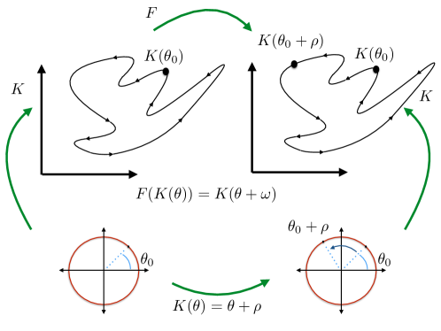
Figure 1: Topological conjugacy to rotation: Here $K\colon\mathbb{S}\to\mathbb{R}^{2}$ is an embedding of the circle. The image of $K$ is invariant under $F$, in the sense that $F\circ K$ is a reparameterization of the curve $K$. In fact, the reparameterization is rotation by an angle $\rho$. The invariance equation $F\circ K=K\circ f$ expresses the fact that the above diagram commutes, meaning that the dynamics on $K$ generated by $F$ are conjugate to the dynamics on the circle generated by $f(\theta)=\theta+\rho$.

Since $\Gamma$ is a smooth curve, the map $K$ is smooth and has convergent Fourier series which we denote by

$$K(\theta)=\begin{pmatrix}K^{1}(\theta)\\ K^{2}(\theta)\end{pmatrix}=\begin{pmatrix}\sum_{n\in\mathbb{Z}}a_{n}e^{2\pi in\theta}\\ \sum_{n\in\mathbb{Z}}b_{n}e^{2\pi in\theta}\end{pmatrix}=\sum_{n\in\mathbb{Z}}\begin{pmatrix}a_{n}\\ b_{n}\end{pmatrix}e^{2\pi in\theta}=\sum_{n\in\mathbb{Z}}k_{n}e^{2\pi in\theta}$$

where

$$k_{n} =\int_{0}^{1}K(\theta)e^{-2\pi in\theta}\,d\theta.$$

The idea is to treat each Fourier coefficient as a 2-vector of observables for the underlying circle map $T$. This can be done, exploiting the fact that Fourier coefficients are defined in terms of integrals and applying the weighted Birkhoff averages of [DSSY16]. Inductively applying Equation (8), we have that

$$p_{k}=F^{k}(p_{0})=F^{k}(K(\theta_{0}))=K(\theta_{k}),$$

with

$$\theta_{k}=\theta_{0}+k\rho,$$

for $k=0,1,2,\ldots,N$. Then

$$k_{n} =\int_{0}^{1}K(\theta)e^{-2\pi in\theta}\,d\theta$$

$$=\lim_{N\to\infty}\sum_{k=0}^{N-1}\hat{w}_{k,N}K(\theta_{k})e^{-2\pi in\theta_{k}}$$

$$=\lim_{N\to\infty}\sum_{k=0}^{N-1}\hat{w}_{k,N}K(\theta_{0}+k\rho)e^{-2\pi in(\theta_{0}+k\rho)}$$

$$=\lim_{N\to\infty}\sum_{k=0}^{N-1}\hat{w}_{k,N}F^{k}(K(\theta_{0}))e^{-2\pi in(\theta_{0}+k\rho)}$$

$$=\lim_{N\to\infty}\sum_{k=0}^{N-1}\hat{w}_{k,N}p_{k}e^{-2\pi in(\theta_{0}+k\rho)}$$

$$=\lim_{N\to\infty}e^{-2\pi in\theta_{0}}\sum_{k=0}^{N-1}\hat{w}_{k,N}p_{k}e^{-2\pi ink\rho}$$

Then

$$k_{n}\approx e^{-2\pi in\theta_{0}}\sum_{k=0}^{N-1}\hat{w}_{k,N}p_{k}e^{-2\pi ink\rho}.$$

The major sources of error in this approximation of the Fourier coefficient $k_{n}$ are threefold. First, the limit as $N\to\infty$ is approximated by computing a finite, rather than an infinite sum. Second, there is the error from the approximated rotation number used to compute the coefficients, that is we use $\rho_{N}$ for some high enough $N$ to approximation $\rho$. Third, the trajectory $\{p_{n}\}_{n=0}^{N}$ is only near a quasiperiodic orbit, generated as it is by numerically iterating the map $F$. Of course, in the end, the parameterization $K$ is approximated using a finite number of Fourier modes.

2.4 The Parameterization Method

The parameterization method is a general functional analytic framework for studying invariant objects in discrete and continuous time dynamical systems. While the method has roots in the classical works of Poincare, Darboux, and Lyapunov, a complete theory for fixed points of infinite dimensional nonlinear maps on Banach spaces emerged in the three papers of Cabré, Fontich, and de la Llave [CFdlL03a, CFdlL03b, CFdlL05]. The corresponding theory for invariant tori (quasi-periodic motions) and their whiskers (stable/unstable fibers) for skew product dynamical systems is developed in the three papers by Haro and de la Llave [HdlL06b, HdlL06a, HdlL07]. Since its introduction in the papers just cited, the method has been expanded and applied by a number of authors, so that a complete overview of the literature is a task beyond the scope of the present work. The interested reader will find an informative and lively discussion of the history of the method in Appendix B of [CFdlL05]. Moreover, the recent book on the topic by Haro, Canadell, Figueras, Luque, and Mondelo [HCF⁺16] contains detailed discussion of the method, a thorough review of the literature, and many detailed example applications.

2.4.1 Parameterization method for an invariant circle in the plane

In the case of invariant circles, the main idea behind the parameterization method is to treat Equation (8) as an equation for an unknown smooth $1$-periodic function $K\colon\mathbb{R}\to\mathbb{R}^{2}$, and to attempt to solve in an appropriate function space via a Newton iteration scheme. Since the Newton method is based in the implicit function theorem, it is essential that we look for an isolated solution of Equation (8). Note however that any rotation of a solution is again a solution, and it is necessary to fix a phase condition to isolate. In the present work we fix the phase by requiring that $K(0)$ lies in a fixed (by us at the outset of the discussion) line in the plane. That is, we choose vectors $\bar{p},\eta\in\mathbb{R}^{2}$ and add the constraint equation

$$\left<\bar{p}-K(0),\eta\right>=0,$$

where $<\cdot,\cdot>$ is the usual inner product in $\mathbb{R}^{2}$. The idea here is that $\bar{p}$ and $\eta$ determine a line $\ell$ transverse to $\Gamma$ and we require $K$ to map $\theta=0$ into the line $\ell$, thus locking down the phase of the parameterization.

The issue now comes when we consider the resulting system of equations

$$F(K(\theta))=K(\theta+\rho).$$

$$\left<\bar{p}-K(0),\eta\right>=0$$

which is clearly two equations in one unknown $K$. To balance the system we introduce a saclar unfolding parameter $\beta$. That is, we consider the system of equations

$$F(K(\theta))=(1+\beta)K(\theta+\rho)$$

$$\left<\bar{p}-K(0),\eta\right>=0,$$

as two equations in two unknowns $K$ and $\beta$. This idea is inspired by similar techniques for balancing the systems of equations describing periodic orbits in Hamiltonian systems. See for example [MnAFG⁺03, MnAGF00]. As with any work involving unfolding parameters, we have to address the relationship between the original unbalanced system of equations and the unfolded system. This is the content of Lemma 2.3, which shows that solutions of the unfolded system satisfy the original equations.

Let $C^{k}_{p}(\mathbb{R})$ denote the space of smooth, period-$1$ functions, with $k>1$. (In our applications $k=\omega$) and define the nonlinear mapping $\Psi\colon\mathbb{R}\times C^{k}_{p}(\mathbb{R})\to\mathbb{R}\times C^{k}_{p}(\mathbb{R})$ by

$$\Psi(\beta,K)=\left(\begin{array}[]{c}\left<\bar{p}-K(0),\eta\right>\\ F(K(\theta))-(1+\beta)K(\theta+\rho)\end{array}\right).$$ (9)

Let $\mathbf{0}$ denote the zero function. We have the following.

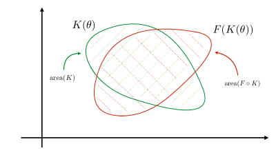
Figure 2: asdaf

Lemma 2.3 ($\beta$ unfolds Equation (9)).

Suppose that $K_{*}\in C_{p}^{k}(\mathbb{R})$ and $\beta_{*}\in\mathbb{R}$ have

$$\Psi(K_{*},\beta_{*})=\left(\begin{array}[]{c}\mathbf{0}\\ 0\end{array}\right).$$

Then $\beta_{*}=0$, and $K$ conjugates the dynamics on $\mbox{image}(K)$ generated by $F$ to the rotation map $R_{\rho}$.

Proof.

Suppose that $K_{*}$ and $\beta_{*}$ provide a zero of $\Psi$. Then

$$F(K_{*}(\theta))=(1+\beta_{*})K_{*}(\theta+\rho).$$ (10)

Let $\Gamma$ denote the curve parameterized by $K_{*}$, and $\tilde{\Gamma}=F\circ\Gamma$ be the curve parameterized by $F\circ K_{*}$. Note that $\tilde{\Gamma}$ is diffeomorphic to $\Gamma$, due to the assumption that $F$ is a diffeomorphism, and that $K_{*}(\theta+\rho)$ is just a reparameterization of the curve $\Gamma$, with different phase.

For $K\in C_{p}^{k}(\mathbb{R})$, consider the integrals

$$A_{1}(K) =\frac{1}{2}\int_{\Gamma}K_{1}\,dy-K_{2}\,dx$$

$$=\frac{1}{2}\int_{0}^{1}\left(K_{1}(\theta)\frac{d}{d\theta}K_{2}(\theta)-K_{2}(\theta)\frac{d}{d\theta}K_{1}(\theta)\right)\,d\theta$$

$$A_{2}(K) =\frac{1}{2}\int_{\Gamma}K_{1}\circ R_{\rho}\,dy-K_{2}\circ R_{\rho}\,dx$$

$$=\frac{1}{2}\int_{0}^{1}\left(K_{1}(\theta+\rho)\frac{d}{d\theta}K_{2}(\theta+\rho)-K_{2}(\theta+\rho)\frac{d}{d\theta}K_{1}(\theta+\rho)\right)\,d\theta$$

and

$$A_{3}(K) =\frac{1}{2}\int_{\tilde{\Gamma}}(F\circ K)_{1}\,dy-(F\circ K)_{2}\circ R_{\rho}\,dx$$

$$=\frac{1}{2}\int_{0}^{1}\left(F(K(\theta)_{1}\frac{d}{d\theta}F(K(\theta)_{2}-F(K(\theta)_{2}\frac{d}{d\theta}F(K(\theta)_{1}\right)\,d\theta.$$

To motivate the consideration of these integrals, we note that if $\Gamma$ is a simple closed curve, then $\tilde{\Gamma}$ is a simple closed curve as well (as $F$ is a diffeomorphism) and $A_{1},A_{2}$ would correspond (by Green’s theorem) to the area enclosed by $\Gamma$. Similarly, $A_{3}$ would be the area enclosed by $\tilde{\Gamma}$. See Figure 2. We remark that $A_{1},A_{2},A_{3}$ are well defined in general as long as $\Gamma$ is closed and , i.e. for all $K$ in $C_{p}^{k}(\mathbb{R})$ with $k>1$, by Greens theorem, and that if the curves have self intersections then the integrals compute enclosed area with overlap.

Moreover, since $A_{1}$ and $A_{2}$ are computed over the same curve (with different parameterizations) we have that

$$A_{1}=A_{2}.$$

Since $\hat{\Gamma}$ is diffeomorphic to $\Gamma$, and $F$ is an area preserving map in the plane (and hence a symplectomorphism) we also have that $A_{1}=A_{3}$.

However, integrating both sides of Equation (10), gives

$$A_{3}(K_{*})=(1+\beta_{*})A_{2}(K_{*}).$$

Combining this with the fact that $A_{2}(K_{*})=A_{1}(K_{*})=A_{3}(K_{*})$, it follows that $\beta_{*}=0$. Heuristically speaking, the area enclosed by $\hat{\Gamma}$ cannot be either more or less then the area enclosed by $\Gamma$ (where overlaps are counted correctly in both cases). From this we obtain that

$$F(K_{*}(\theta))=K_{*}(\theta+\rho),$$

and hence $K_{*}$ conjugates the dynamics on $\Gamma$ to the irrational rotation $R_{\rho}$.

∎

2.5 Newton scheme in Fourier coefficient space

Fortified by Lemma 2.3, we now seek to solve the Equation $\Psi(K,\beta)=0$, as defined in Equation (9) for the unknown parameterization $K$. Indeed suppose that $K_{0}$ is an approximate zero of the equation and and choose $\beta_{0}=0$. The Newton sequence is given by

$$\left(\begin{array}[]{c}\beta_{n+1}\\ K_{n+1}\end{array}\right)=\left(\begin{array}[]{c}\beta_{n}\\ K_{n}\end{array}\right)+\left(\begin{array}[]{c}\delta_{n}\\ \Delta_{n}\end{array}\right),\quad\quad n\geq 0,$$

where $(\delta_{n},\Delta_{n})^{T}$ is a solution of the linear equation

$$D\Psi(\beta_{n},K_{n})\left(\begin{array}[]{c}\delta_{n}\\ \Delta_{n}\end{array}\right)=-\Psi(\beta_{n},K_{n}).$$ (11)

Here, for $\beta,\delta\in\mathbb{R}$ and $K,\Delta\in C_{p}^{k}(\mathbb{R})$ the Frechet derivative of $\Psi$ has action

$$D\Psi(\beta,K)\left(\begin{array}[]{c}\delta\\ \Delta\end{array}\right)=\left(\begin{array}[]{c}-\left<\Delta(0),\eta\right>\\ -\delta K(\theta+\rho)+DF(K(\theta))\Delta(\theta)-(1+\beta)\Delta(\theta+\rho)\end{array}\right).$$

Remark 2.4 (Fast algorithms exploiting the symplectic structure).

The efficiency of the Newton scheme is improved dramatically via the area preserving/symplectic structure of the problem, which facilitates reduction of the linear equation (11) to constant coefficient, plus a quadratically small error. This idea is known in the literature as approximate reducibility. Neglecting the quadratic error, the resulting constant coefficient linear equations are easily diagonalized (in Fourier coefficient space). The reader interested in state of the art algorithms is referred to[CCH21, CF12, HM21, CCdlL22, GHdlL22] We again refer to [HCF⁺16] for comprehensive discussion.

Since we seek periodic $K$ it is natural to write make the Fourier ansatz

$$K(\theta)=\sum_{n\in\mathbb{Z}}\left(\begin{array}[]{c}a_{n}\\ b_{n}\end{array}\right)e^{2\pi in\theta},$$

as considered already in Section 2.3.1. Note that translation by $\rho$ is a diagonal operation in Fourier space, as

$$K(\theta+\rho) =\sum_{n\in\mathbb{Z}}\left(\begin{array}[]{c}a_{n}\\ b_{n}\end{array}\right)e^{2\pi in(\theta+\rho)}$$

$$=\sum_{n\in\mathbb{Z}}e^{2\pi in\rho}\left(\begin{array}[]{c}a_{n}\\ b_{n}\end{array}\right)e^{2\pi in\theta},$$

and that the phase condition can be written as

$$\left<\bar{p}-K(0),\eta\right>=\bar{p}_{1}\eta_{1}+\bar{p}_{2}\eta_{2}-\sum_{n\in\mathbb{Z}}\left(\eta_{1}a_{n}+\eta_{2}b_{n}\right).$$

The nonlinearity is more complicated, but note that if $K\in C_{p}^{k}$ then $F\circ K\in C_{p}^{k}$ as well, assuming that $F$ is as smooth as $K$. (For the examples in this paper $F$ is real analytic). Then $F\circ K$ has Fourier expansion

$$F(K(\theta))=\sum_{n\in\mathbb{Z}}(F\circ K)_{n}e^{2\pi in\theta},$$

where the Fourier coefficients $(F\circ K)_{n}$ depend in a nonlinear way way on the Fourier coefficients $a_{n},b_{n}$. In practice if $F$ is a polynomial map then this dependence is worked out by discrete convolutions, as seen in the examples. Otherwise, the map is computed numerically using the FFT. Indeed, using the FFT, evaluation of the nonlinearity is a diagonal operation in grid space.

2.6 Multiple shooting for period-$d$ systems of invariant circles

We now consider a “multiple-shooting” parameterization method for studying $d$-periodic systems of quasi-periodic invariant sets. Such a set is the union of $d$ disjoint simple closed curves, with the property each point on one curve maps to another curve in the system. The dynamics are required to be quasi-periodic. More precisely, suppose that $\Gamma_{1},\ldots,\Gamma_{d}\subset\mathbb{R}^{2}$ are smooth simple closed curves with

$$F(\Gamma_{1}) =\Gamma_{2}$$ (12)

$$F(\Gamma_{2}) =\Gamma_{3}$$ (13)

$$\vdots$$ (14)

$$F(\Gamma_{d-1}) =\Gamma_{d}$$ (15)

$$F(\Gamma_{d}) =\Gamma_{1}.$$ (16)

Suppose moreover that, for each $1\leq j\leq d$, the curve $\Gamma_{j}$ is quasi-periodic for the composition map $F^{d}$. That is, suppose that for each $1\leq j\leq d$ the mapping $F^{d}$ restricted to $\Gamma_{j}$ is an orientation preserving circle homeomorphism with irrational rotation number $\rho_{j}$. The situation is illustrated in Figure 3.

Note that compositions of $F$ provide conjugacies between each of the $F^{d}$ invariant circles $\Gamma_{j}$. For example, the map $F$ provides a conjugacy between the dynamics on $\Gamma_{j}$ and $\Gamma_{j+1}$ while $F^{2}$ conjugates $\Gamma_{j}$ to $\Gamma_{j+2}$ and so on. Then, since $F$ is a diffeomorphism (and hence a homeomorphism), the topological invariance of the rotation number gives that $\rho_{1}=\ldots=\rho_{j}$, and it is permissible to simply write $\rho$ for the common rotation number.

One computational approach for studying this invariant set would be to apply the parameterization discussed in Section 2.4.1 to the map $F^{N}$, once for each of the curves $\Gamma_{j}$, $1\leq j\leq d$. This approach however has two major disadvantages: first, the computational complexity of the composition map evaluation grows exponentially with the number of compositions. For example if $F$ is polynomial of degree $m$ then $F^{2}$ is polynomial of degree $m^{2}$ and $F^{d}$ is polynomial of degree $m^{d}$. The second disadvantage is that one has to compute parameterizations of $\Gamma_{1},\ldots,\Gamma_{d}$ separately.

Instead, we propose a “multiple shooting” parameterization method for computing the entire period period $d$ systems of quasiperiodic curves all at once. Earlier successful multiple shooting approaches are developed in the work of [GMJ17] for parameterizing stable/unstable manifolds attached to period-$d$ orbits of maps, and in the [TMJ22] for studying invariant objects for discrete dynamical systems defined by an implicit rule. In the current context we look for smooth parameterizations $K_{1},\ldots,K_{d}\colon\mathbb{R}\to\mathbb{R}^{2}$ – all of period one – so that for each $\theta\in\mathbb{R}$ we have that

$$F(K_{1}(\theta)) =K_{2}(\theta)$$

$$F(K_{2}(\theta)) =K_{3}(\theta)$$

$$\vdots$$

$$F(K_{d-1}(\theta)) =K_{d}(\theta)$$

$$F(K_{d}(\theta)) =K_{1}(\theta+\rho),$$

where $\rho$ is the rotation number associated with any of the invariant circles of the composition map $F^{d}$.

Once again, it is necessary to append a scalar constraint to fix the phase of one of the circles – this in turn fixes the phase of each parameterization. Appending the phase constraint unbalances the system so that it is necessary to introduce an unfolding parameter. Taking these considerations into account, we define the operator $\Psi_{d}\colon\mathbb{R}\times C_{d}^{k}(\mathbb{R},\mathbb{R^{2}})^{d}\to\mathbb{R}\times C_{d}^{k}(\mathbb{R},\mathbb{R^{2}})^{d}$, defined by

$$\Psi_{d}(\beta,K_{1},K_{2},K_{3},\ldots,K_{d-1},K_{d})=\left(\begin{array}[]{c}\left<K_{1}(0)-\bar{p},\eta\right>\\ F(K_{1}(\theta))-K_{2}(\theta)\\ F(K_{2}(\theta))-K_{3}(\theta)\\ \vdots\\ F(K_{d-1}(\theta))-K_{d}(\theta)\\ F(K_{d}(\theta))-(1+\beta)K_{1}(\theta+\rho),\end{array}\right)$$ (17)

Again, the important thing to stress if that the definition of $\Psi_{d}$ does in to involve any compositions of the map $F$. A Newton method is defined as in Section 2.5.

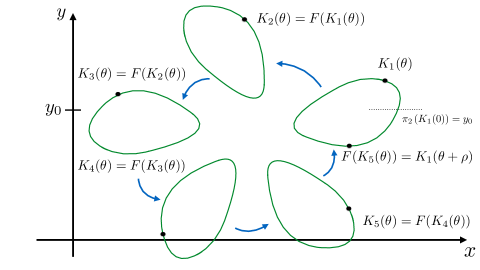
Figure 3: Schematic illustration of a period $5$ invariant circle and the resulting parameterization method.

3 Numerical recipe: initializing the parameterization method via weighted averaging

Suppose that $\Omega\subset\mathbb{R}^{2}$ is an open set and let $F\colon\Omega\to\Omega$ be a smooth, area preserving map. The following algorithm (i) allows us to determine that we have an initial condition whose orbit is very likely one or near a quasiperiodic invariant circle, (ii) allows us to compute the rotation number efficiently and accurately from just the orbit segment data, (iii) allows us to easily determine the truncation dimension for the finite dimensional Fourier projection of the parameterization, (iv) leads in a completely natural way to an initial guess for the parameterization method which can be made as accurate as we like – hence will definitely converge. We also (v) have an a-posteriori indicator which allows us to decide when Newton has converged. The following steps constitute the main steps of our algorithm.

• Step 0: choose $p_{0}=(x_{0},y_{0})\in\Omega$ and $M\in\mathbb{N}$. Compute the orbit segment $\mathcal{O}_{M}=\{p_{j}\}_{j=0}^{M}$ defined by

  $$p_{j+1}=F(p_{j}),\quad\quad\quad j\in 1,\ldots,M-1.$$

  Now, decide if $\mathcal{O}_{M}$ is sampled from an invariant circle, or from a stochastic zone. This can be done either by graphical inspection, or using the techniques of [SM20, MS21] already mentioned in Remark 2.1. If $\mathcal{O}_{M}$ appears to be sampled from a quasiperiodic invariant circle, then we continue to the next step. Otherwise, choose a different $p_{0}$.

• Step 1: Compute the rotation number $\rho$ using the weighted averaging technique discussed in Section 2.3. Here it is important to obtain as many correct digits as possible. This can be done by increasing $M$ by ten or twenty percent and repeating the calculation until numerical convergence in the last digit is observed.

• Step 2: Decide how many modes are needed to accurately represent $K$. To do this, we compute the Fourier coefficients $(a_{n},b_{n})$ using the averaging scheme described in Section 2.3.1. However we compute using a much shorter sample (that is we use $M$ much smaller than in the rotation number calculation) and sample the modes by computing them only for $n=10k$, and $k=1,2,3,\ldots$. Using this scheme we can rapidly find an $N\in\mathbb{N}$ so that $\|(a_{n},b_{n})\|<\epsilon_{{\tiny\mbox{machine}}}$ for $|n|>N$.

• Step 3: We now calculate a good initial condition for the Newton scheme. For this we take $N_{0}$ roughly ten or twenty percent of $N$ and compute $(a_{n},b_{n})$, using moderate accuracy (i.e. $M$ larger than in step 2 but smaller than in step 1), for $|n|\leq N_{0}$ using the weighted averages of Section 2.3.1. Let’s call the resulting degree $N_{0}$ Fourier polynomial $\tilde{K}$. Compute the numerical defect

  $$\tilde{\epsilon}=\sup_{\theta\in[0,1]}\left|F(\tilde{K}(\theta))-\tilde{K}(\theta+\rho)\right|.$$

  If $\tilde{\epsilon}$ is smaller than some tolerance – which should be less than one but is usually taken to be between $0.001$ and $0.1$, depending on the judgment of the user – then the initial guess is “good” and we set $K_{0}=\tilde{K}$. If the initial defect is not good enough, then we can increase $N_{0}$ and try again.

• Step 4: Perform the Newton iteration (in the space of $N$-Fourier coefficients) as described in Section 2.5. Iterate the Newton scheme until the defect

  $$\epsilon_{m}=\sup_{\theta\in[0,1]}\left|F(K_{m}(\theta))-K_{m}(\theta+\rho)\right|,$$

  either saturates or decreases below some prescribed tolerance (usually taken to be some small multiple of machine epsilon).

Several remarks are in order. First, we note that the $C^{0}$ norm proposed for measuring the defect in Steps $3$ and $4$ can be replaced with more efficient weighted $\ell_{1}$ norms, and this involves computations only in coefficient space rather than function evaluations. We also remark that if the Newton scheme does not converge in Step $4$, then we conclude that the initial defect was not good enough and go back to step $3$ to refine $N_{0}$.

It should also be noted that the defect calculations proposed above provide only a heuristic indication of convergence. More reliable error bounds for the parameterization method, based on a-posteriori Kantorovich-type results, are obtained in [HdlL06b]. See also [HCF⁺16]. Indeed, this kind of a-posteriori analysis can be combined with deliberate control of round of errors to obtain mathematically rigorous computer assisted existence proofs. Early examples of this kind of argument are found in the work of [dlLR91, dlLR90]. For a more modern treatment, including a thorough discussion of the current state of the literature, we refer the interested reader to the work of [FHL17].

4 Examples

4.1 A quadratic family of maps: area preserving Henon

As a first example, consider the area-preserving Hénon map, $F:\mathbb{R}^{2}\to\mathbb{R}^{2}$ as described in [Han69], and given by the formula

$$F(x,y)=\left(\begin{array}[]{c}x\cos(\alpha)-(y-x^{2})\sin(\alpha)\\ x\sin(\alpha)+(y-x^{2})\cos(\alpha)\end{array}\right).$$

One checks that the determinant of the Jacobian matrix $DF(x,y)$ is one for all $(x,y)\in\mathbb{R}^{2}$, so that the system is area preserving as advertised. The dynamics of the system are studied for a number of parameter values $\alpha$ in the book of [APP90]. In particular, numerical simulations suggest that the system appears to admit quasiperiodic invariant circles and $K$-periodic systems of such. The map can be seen as a linear rotation matrix at the origin, plus a quadratic nonlinearity. There is one (and only one) fixed point –at the origin and of elliptic stability type – so that in a small enough neighborhood of the origin we expect the existence of large measure sets of KAM tori. This expectation is supported by numerical simulations, as seen for example in Figure 4. for $\alpha=\cos^{-1}(0.24)$.

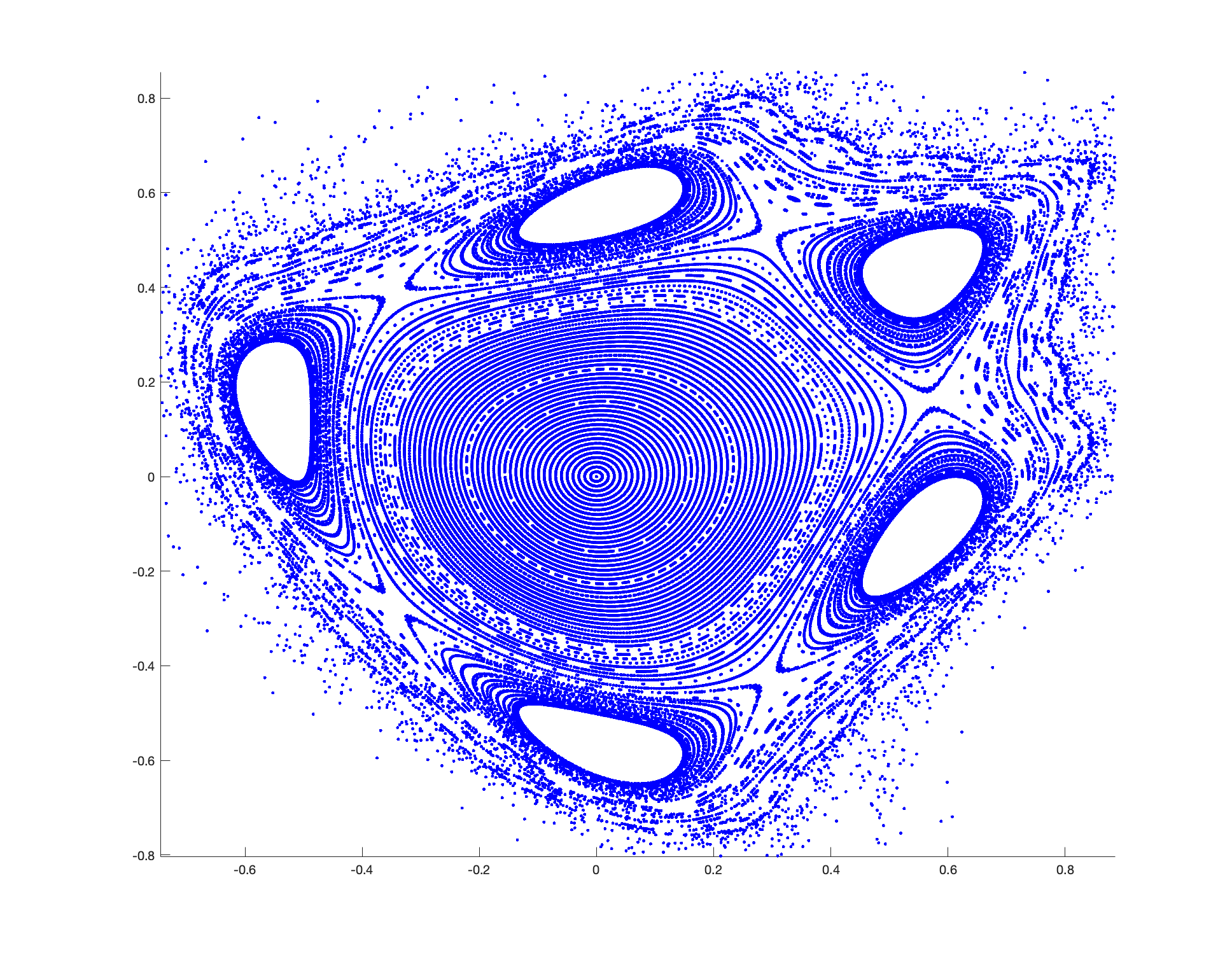
Figure 4: Phase space structure for the area preserving Henon map: near the origin the dynamics are close to pure rotation and we see a large set of invariant circles. These get more and more distorted further from the origin, and eventually there appears to be a $1:5$ resonance which gives rise to a family of systems of invariant circles with $5$ topological components. Further from the origin the dynamics appears to be chaotic.

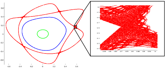
Figure 5: Three orbits: one million iterates of the area preserving Henon map for the three initial conditions $\mathbf{p_{0}}=(0.1,0.0)$, $\mathbf{p_{0}}=(0.4,0.0)$ and $\mathbf{r_{0}}=(0.3,0.44)$. (green, blue and red respectively). Visual inspection suggests that the green and blue curves are diffeomorphic to circles, while zooming in on the point cloud generated by the orbit of $\mathbf{r}_{0}$ reveals fractal structure and suggests chaotic dynamics. This suggestion is enforced by the quantitative data in Table 1.

$M$	$\rho_{M}(\mathbf{p_{0}})$	$\rho_{M}(\mathbf{q}_{0})$	$\rho_{M}(\mathbf{r}_{0})$
100	0.211095710088270	0.206164038365342	0.196863099485937
500	0.211095709965501	0.206174513248940	0.197503558666674
1000	0.211095709965479	0.206174514865070	0.197628415757003
5000	0.211095709965481	0.206174514865715	0.199431995293399
10,000	0.211095709965478	0.206174514865712	0.199737097322017
50,000	0.211095709965486	0.206174514865718	0.199823145343572
100,000	0.211095709965480	0.206174514865710	0.199984739391916
110,000	0.211095709965478	0.206174514865708	0.199990822989916
120,000	0.211095709965479	0.206174514865704	0.199994461862213
150,000	0.211095709965479	0.206174514865705	0.199998753698169
200,000	0.211095709965478	0.206174514865702	0.199999888701773

Table 1: Numerically computed values of the rotation number as a function of $M$ for the three initial conditions $p_{0}$, $q_{0}$, and $r_{0}$. This is denoted $\rho_{M}(\cdot)$, where $\cdot$ is one of the initial conditions and $M$ between one hundred and and two hundred thousand. The computations suggest that the orbits of $p_{0}$ and $q_{0}$ are quasiperiodic, while the rotation number of the orbit of $r_{0}$ varies stochastically after the 4th digit.

4.1.1 A worked example: period 1 invariant circle

We now describe in some detail the computation of a period one invariant circle for the area preserving Henon map.

• Step 0: consider the three initial conditions $p_{0},q_{0},r_{0}\in\mathbb{R}^{2}$ given by

  $$p_{0}=\left(\begin{array}[]{c}0.1\\ 0.0\end{array}\right),\quad\quad q_{0}=\left(\begin{array}[]{c}0.4\\ 0.0\end{array}\right),\quad\quad\mbox{and}\quad\quad r_{0}=\left(\begin{array}[]{c}0.3\\ -0.44\end{array}\right).$$

  One million iterates of each initial condition are illustrated in Figure 5, with a zoom in on the orbit of $r_{0}$, illustrating that the orbit appears to be chaotic rather than quasiperiodic. This appearance is confirmed by the rotation number calculations given in Table 1. Based on these results, and for the rest of the Section, we focus on the orbit of $q_{0}$.

• Step 1: Based on the results of step 0, since we can say with confidence that the rotation number associated with the orbit of $q_{0}$ has

  $$\rho\approx\rho_{120,000}=0.206174514865704,$$

  which is likely correct except possibly in the last decimal place.

• Step 2: Using the rotation number computed in the last step, we sample the Fourier coefficients in the higher modes. We note that with $M=1,000$ we already appeared to have seven correct figures in the rotation number calculation. So we will compute Fourier coefficients with an orbit of only this length. Let $p_{n}=(a_{n},b_{n})$ denote the $n$-th Fourier vector and

  $$\|p_{n}\|=\max(|a_{n}|,|b_{n}|),$$

  with $|\cdot|$ the complex absolute value. Sampling the coefficients for $n=2,4,6,8,10,$ we have

  $$\|p_{2}\| =2.0\times 10^{-2}$$

  $$\|p_{4}\| =4.3\times 10^{-3}$$

  $$\|p_{6}\| =6.5\times 10^{-4}$$

  $$\|p_{8}\| =4.8\times 10^{-5}$$

  $$\|p_{10}\| =8.4\times 10^{-6}$$

  Based on the observed decay rate, we guess that we should reach machine precision at roughly $n=30$. Being a little conservative, we take $K=5$ and truncate to $N=2^{K}=32$ Fourier modes. (Powers of 2 are desirable if the implementation emploies the FFT).

• Step 3: . We now compute the Fourier series for $N_{0}=5$, from 10,000 data points. This is about 10 percent of the modes to be Used in the Newton scheme. This leads to a trigonometric polynomial that we refer to as

  $$\tilde{K}(\theta)=\sum_{n=-5}^{5}\left(\begin{array}[]{c}a_{n}\\ b_{n}\end{array}\right)e^{2\pi in\theta}.$$

  Then initial defect associated with this approximate solution is already $\epsilon\leq 9.2\times 10^{-4}$. We therefore consider this a good initial approximation and define $K_{0}=\tilde{K}$.

• Step 4: We run the newton iteration and obtain defects

  $$\epsilon_{1}=2.2\times 10^{-6}$$

  $$\epsilon_{2}=4.1\times 10^{-12}$$

  $$\epsilon_{3}=6.1\times 10^{-13}$$

  $$\epsilon_{4}=6.0\times 10^{-13}$$

  and the conjugacy error stagnates. The Newton scheme executes in $0.062$ seconds. Running again from the same initial condition $K_{0}$ with $N=64$, the next power of two Fourier modes, results in a final conjugacy error of $\epsilon=1.6\times 10^{-14}$ and takes $0.18$ seconds. The next power $N=128$ takes $0.38$ seconds and results in a conjugacy error of $\epsilon=6.1\times 10^{-16}$, which is finally on the order of double precision Machine epsilon. Truncating at $N=256$ Fourier coefficients results in a $0.9$ second runtime, and does not improve the conjugacy error. Indeed, we see that the initial $N=32$ calculation was already nearly optimal.

We provide a few additional details regarding the numerical implementation in this example. Let $a=\{a_{n}\}_{n\in\mathbb{Z}}$ and $b=\{b_{n}\}_{n\in\mathbb{Z}}$ denote the unknown Fourier series coefficients for the parameterization $K$. Then

$$F(K(\theta))=\sum_{n\in\mathbb{Z}}\left(\begin{array}[]{c}\cos(\alpha)a_{n}-\sin(\alpha)b_{n}+\sin(\alpha)(a*a)_{n}\\ \sin(\alpha)a_{n}+\cos(\alpha)b_{n}-\cos(\alpha)(a*a)_{n}\end{array}\right)e^{2\pi in\theta},$$

where

$$(a*a)_{n}=\sum_{k\in\mathbb{Z}}a_{n-k}a_{k},$$

denotes discrete convolution. Recalling that

$$K(\theta+\rho)=\sum_{n\in\mathbb{Z}}e^{2\pi in\rho}\left(\begin{array}[]{c}a_{n}\\ b_{n}\end{array}\right)e^{2\pi in\theta},$$

then the unfolded conjugacy equation $F(K(\theta))=(1+\beta)K(\theta+\rho)$ is satisfied if and only of the Fourier coefficients on the left equal the Fourier coefficients on the right, and we require that

$$\left(\begin{array}[]{c}\cos(\alpha)a_{n}-\sin(\alpha)b_{n}+\sin(\alpha)(a*a)_{n}\\ \sin(\alpha)a_{n}+\cos(\alpha)b_{n}-\cos(\alpha)(a*a)_{n}\end{array}\right)=(1+\beta)e^{2\pi in\rho}\left(\begin{array}[]{c}a_{n}\\ b_{n}\end{array}\right)\quad\mbox{for }n\in\mathbb{Z}.$$ (18)

Moreover, noting that the invariant circle given by the data crosses the $x$-axis we choose the phase condition

$$K_{2}(0)=\sum_{n\in\mathbb{Z}}b_{n}=0.$$

Truncating at $N$ Fourier modes leads to the system of $2(2N+1)+1$ equations

$$b_{-N}+\ldots+b_{0}+\ldots b_{N} =0$$

$$\cos(\alpha)a_{-N}-\sin(\alpha)b_{-N}+\sin(\alpha)(a*a)^{N}_{-N}-(1+\beta)e^{-2\pi iN\rho}a_{-N} =0$$

$$\sin(\alpha)a_{-N}+\cos(\alpha)b_{-N}-\cos(\alpha)(a*a)^{N}_{-N}-(1+\beta)e^{-2\pi iN\rho}b_{-N} =0$$

$$\vdots$$

$$\cos(\alpha)a_{0}-\sin(\alpha)b_{0}+\sin(\alpha)(a*a)^{N}_{0}-(1+\beta)a_{0} =0$$

$$\sin(\alpha)a_{0}+\cos(\alpha)b_{0}-\cos(\alpha)(a*a)^{N}_{0}-(1+\beta)b_{0} =0$$

$$\vdots$$

$$\cos(\alpha)a_{N}-\sin(\alpha)b_{N}+\sin(\alpha)(a*a)^{N}_{N}-(1+\beta)e^{2\pi iN\rho}a_{N} =0$$

$$\sin(\alpha)a_{N}+\cos(\alpha)b_{N}-\cos(\alpha)(a*a)^{N}_{N}-(1+\beta)e^{2\pi iN\rho}b_{N} =0$$

in the $2(2N+1)+1$ unknowns $\beta,a_{-N},b_{-N},\ldots,a_{0},b_{0},\ldots,a_{N},b_{N}$. Here

$$(a*a)_{n}^{N}=\sum_{\stackrel{{\scriptstyle k_{1}+k_{2}=n}}{{-N\leq k_{1},k_{2}\leq N}}}a_{k_{1}}a_{k_{2}},$$

is the truncated discrete convolution. Newton’s method is used to solve this system.

A higher level representation is obtained as follows. Let $a=\{a_{n}\}_{n\in\mathbb{Z}}$ and $b=\{b_{n}\}_{n\in\mathbb{Z}}$ denote the unknown sequences of Fourier coefficients and define the “diagonal” linear operator $R_{\rho}$ on an infinite sequence by

$$(R_{\rho}a)_{n}=e^{2\pi in\rho}a_{n}.$$ (19)

Inspired by the conditions given in Equation (18), we define the mapping

$$\mathcal{F}(\beta,a,b)=\left(\begin{array}[]{c}\sum_{n\in\mathbb{Z}}b_{n}\\ \cos(\alpha)a-\sin(\alpha)b+\sin(\alpha)a*a-(1+\beta)R_{\rho}a\\ \sin(\alpha)a+\cos(\alpha)b-\cos(\alpha)a*a-(1+\beta)R_{\rho}b\end{array}\right),$$

and seek a zero of $F$. Note that, for numbers $\delta$ and infinite sequences $u,v$, we see that the action of the (formal) Frechet derivative on $(\delta,u,v)$ is given by

$$D\mathcal{F}(\beta,a,b)(\delta,u,v)=\left(\begin{array}[]{c}\sum_{n\in\mathbb{Z}}v_{n}\\ \cos(\alpha)u-\sin(\alpha)v+2\sin(\alpha)a*u-(1+\beta)R_{\rho}u-R_{\rho}a\\ \sin(\alpha)u+\cos(\alpha)v-2\cos(\alpha)a*u-(1+\beta)R_{\rho}v-R_{\rho}b\end{array}\right).$$

A more useful is the following expression for the derivative as a “matrix of operators.”

Let $\mathbf{0}$ denote the zero Fourier sequence and $\mathbf{1}$ the sequence of ones. Moreover, let $\mathbf{R}_{\rho}$ denote the bi-infinite diagonal matrix with $e^{2\pi in\rho}$ on the diagonal entries, and let $\mathbf{S}_{\alpha},\mathbf{C}_{\alpha}$ denote the bi-infinite diagonal matrices with $\sin(\alpha)$ and $\cos(\alpha)$ on their diagonals respectively. Finally, let $\mathbf{A}$ denote the (dense) bi-infinite matrix defined by the linear mapping

$$\mathbf{A}h=a*h.$$

The matrix for $A$ is easily worked out by considering it’s action on the basis for bi-infinite sequence space given by sequences with on one non-zero entry. The classical result is that $A$ is a Topoletz matrix for the bi-infinite sequence $a$. Then the derivative can be represented as

$$D\mathcal{F}(\beta,a,b)=\left(\begin{array}[]{ccc}0&\mathbf{0}&\mathbf{1}\\ -\mathbf{R}_{\rho}a&\mathbf{C}_{\alpha}+2\mathbf{C}_{\alpha}\mathbf{A}-(1+\beta)\mathbf{R}_{\rho}&-\mathbf{S}_{\alpha}\\ -\mathbf{R}_{\rho}b&\mathbf{S}_{\alpha}-2\mathbf{C}_{\alpha}\mathbf{A}&\mathbf{C}_{\alpha}-(1+\beta)\mathbf{R}_{\rho}\end{array}\right).$$

Truncating the mapping $\mathcal{F}$ and its derivative given above leads to a numerical implementation of the Newton scheme.

4.2 Period $K$ circles in Hénon

Another apparent feature of the phase space readily visible in Figure 4, is what looks like a family of period 5 invariant circles. After visual inspection of the figure, we plot a trajectory using $(x_{0},y_{0})=(0.5,0)$ as our seed point, and observe that after 1000 iterates, the orbit appear to fill out the five circles shown in the left frame of Figure 6. We remark that each iterate jumps from one circle to the next circle to its left (counter clockwise rotation).

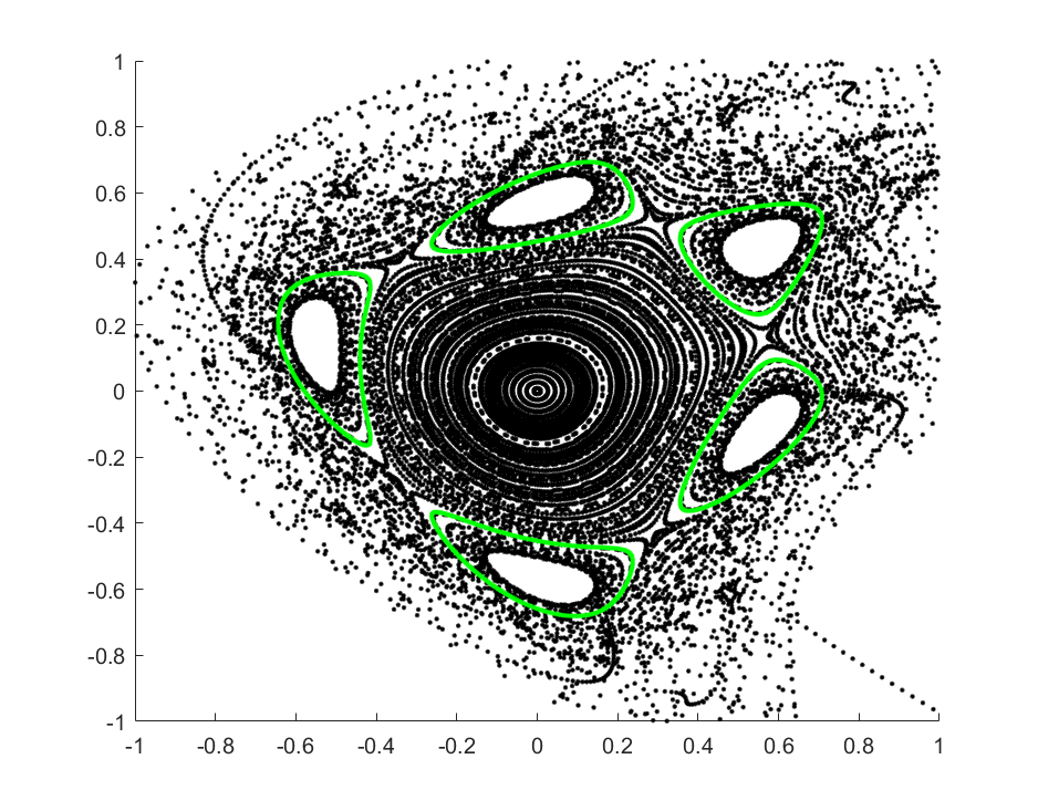
Figure 6: A period five system of quasiperiodic invariant circles: left frame illustrates a numerical simulation of the area preserving system, and an orbit which appears to lie on the period 5 system of invariant circles. The right frame illustrates the image of the five Fourier series parameterizing the quasiperiodic system.

4.2.1 Multiple shooting invariance equations

The idea is to follow the steps proposed in Section 3, with a few small modifications. After guessing a point on the period $5$ system, we compute an orbit segment for the fifth iterate of $F$, denoted $F^{5}$, and compute the rotation number for the composition. This means that if we desire an orbit segment of length $M$, we have to iterate $F$ $5M$ times. Since all $5$ circles have the same rotation number, this only has to be done once. Using the Birkhoff averages with an orbit segment of length $5\times 9,000$ leads to $\rho=0.190669478955264$ which has stabilized numerically to the last digit.

Now let $K_{1},K_{2},K_{3},K_{4},K_{5}\colon\mathbb{R}\to\mathbb{R}^{2}$ denote the desired parameterizations for the five component circles of the system. We use the weighted Birkhoff averages to compute (roughly) the decay rate of these Fourier series (to guess that the optimal truncation order is around $N=200$) and to approximate the first few Fourier coefficients in each case. Again, for this work we deal only with (shorter) orbit segments for the composition map $F^{5}$. We stress that this just requires computing a long enough orbit for $F$ and then neglecting all but every fifth point on the orbit.

Now, when it comes to the Newton method we work with multiple shooting system of equations, so that the nonlinearity is still only quadratic (note that $F^{5}$ is a polynomial map of degree $2^{5}=32$). Keeping in force the notation from Section 4.1.1, we define the mapping

$$\mathcal{F}_{5}(\beta,a^{1},b^{1},a^{2},b^{2},a^{3},b^{3},a^{4},b^{4},a^{5},b^{5})=$$

$$\left(\begin{array}[]{c}\sum_{n\in\mathbb{Z}}b^{1}_{n}\\ \cos(\alpha)a^{1}-\sin(\alpha)b^{1}+\sin(\alpha)a^{1}*a^{1}-R_{\rho}a^{2}\\ \sin(\alpha)a^{1}+\cos(\alpha)b^{1}-\cos(\alpha)a^{1}*a^{1}-R_{\rho}b^{2}\\ \cos(\alpha)a^{2}-\sin(\alpha)b^{2}+\sin(\alpha)a^{2}*a^{2}-R_{\rho}a^{3}\\ \sin(\alpha)a^{2}+\cos(\alpha)b^{2}-\cos(\alpha)a^{2}*a^{2}-R_{\rho}b^{3}\\ \cos(\alpha)a^{3}-\sin(\alpha)b^{3}+\sin(\alpha)a^{3}*a^{3}-R_{\rho}a^{4}\\ \sin(\alpha)a^{3}+\cos(\alpha)b^{3}-\cos(\alpha)a^{3}*a^{3}-R_{\rho}b^{4}\\ \cos(\alpha)a^{4}-\sin(\alpha)b^{4}+\sin(\alpha)a^{4}*a^{4}-R_{\rho}a^{5}\\ \sin(\alpha)a^{4}+\cos(\alpha)b^{4}-\cos(\alpha)a^{4}*a^{4}-R_{\rho}b^{5}\\ \cos(\alpha)a^{5}-\sin(\alpha)b^{5}+\sin(\alpha)a^{5}*a^{5}-(1+\beta)R_{\rho}a^{1}\\ \sin(\alpha)a^{5}+\cos(\alpha)b^{5}-\cos(\alpha)a^{5}*a^{5}-(1+\beta)R_{\rho}b^{1}\\ \end{array}\right),$$

and have that if $(\beta,a_{1},b_{1},a_{2},b_{2},a_{3},b_{3},a_{4},b_{4},a_{5},b_{5})$ is a zero of $\mathcal{F}_{5}$, then $\beta=0$ the $a^{\prime}s$ and $b^{\prime}s$ are the Fourier coefficient sequences of the parameterizations $K_{1},K_{2},K_{3},K_{4}$, and $K_{5}$ for the system of invariant circles. Note that while the map has more components, the nonlinearity is still only as complicated as that of $F$. In this case quadratic. The derivative of $\mathcal{F}$ is easily computed. Truncating the map and its derivative leads to the numerical implementation of the Newton method. Note that all the operations and linear operators are as in the case of a period one circle. Only the number of components and the coupling is different. After implementing these adjustments we are able to compute the parameterizations to machine precision as in the earlier example. The resulting Fourier series are plotted in the right Frame of Figure 6.

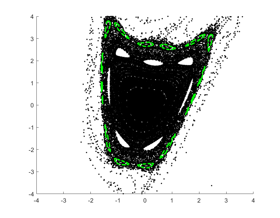
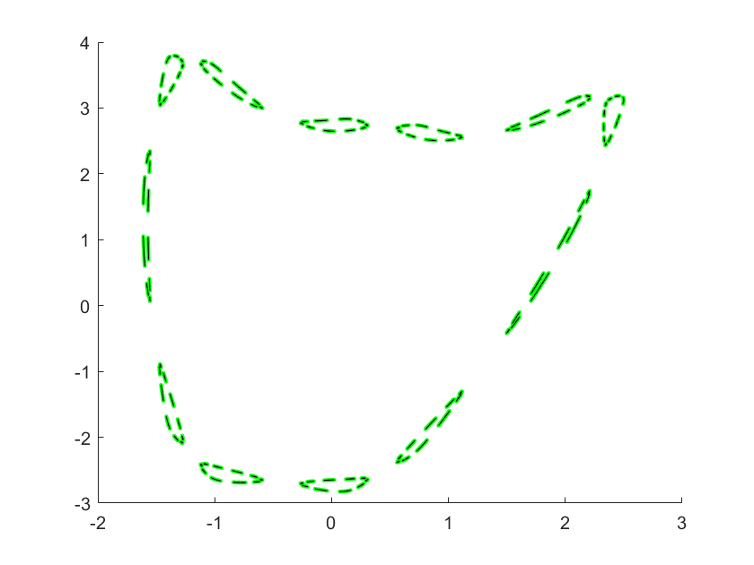
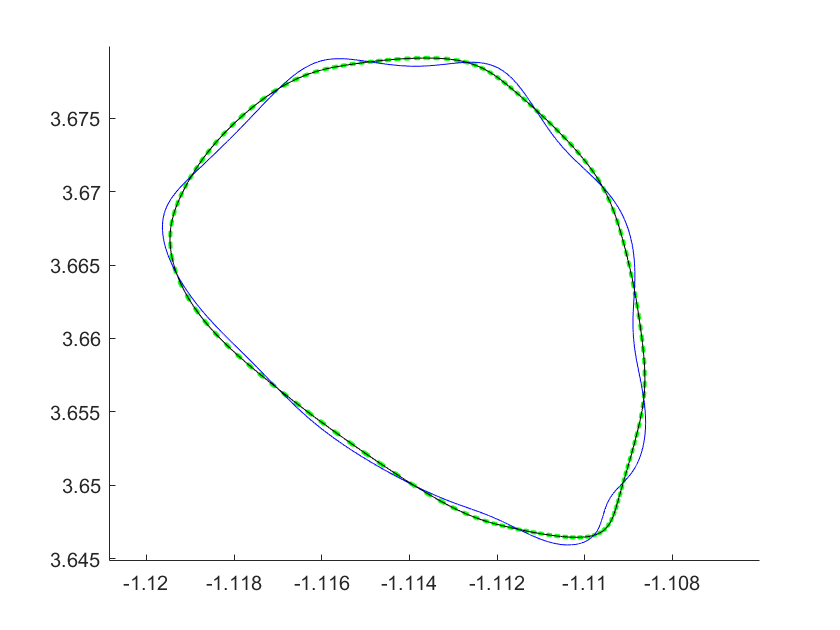
Figure 7: A period 120 system of quasiperiodic invariant circles: left frame is the phase space simulation and orbit data. Middle frame illustrated the images of Fourier parameterizations. Right frame is a close up of the initial and final parameterizations of a single component circle.

The phase space for the area preserving Henon when $\alpha=\arccos(-0.95)$ is illustrated in the left frame of Figure 7, and there is the suggestion of even longer systems of invariant circles. For example, repeating the procedure discussed in the proceeding section using the initial condition $(x_{0},y_{0})=(0,-2.65)$ leads to the period 120 system of quasiperiodic invariant circles illustrated in the left frame of Figure 7. The Fourier mapping $\mathcal{F}_{120}$ generalizes from $\mathcal{F}_{5}$ in the obvious way. Fortunately, the individual circles are not terribly complicated harmonically, and $15$ modes per circle appears to be enough to approximate the Fourier expansions well. Again, the Newton method converges with and we obtain the parameterizations $K_{1},\ldots,K_{120}$ whose images are illustrated in the center frame of Figure 7. The right frame illustrates the initial and final parameterizations at a zoom in on one of the 120 components.

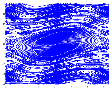
Figure 8: Phase space structure for the standard map with $\alpha=\pi/4$: in the simulation illustrated in this figure, we have taken the first component modulo $2\pi$ so the line at $x=0$ is identified with the line at $x=2pi$. This has the effect of making the phase space into a cylinder, and there are primary invariant tori which appear as smooth curves running from left to right. In the present work however, we study the secondary tori associated with the elliptic fixed point at $(\pi,0)$. These tori are visible wether or not we compute modulo $2pi$.

4.3 Computations for the Standard Map

For an example of a map with non-polynomial nonlinearity, consider the Standard Map of [Chi79]. Since we are interested in secondary (contractable) invariant tori, we treat the map as a diffeomorphism $F:\mathbb{R}^{2}\to\mathbb{R}^{2}$ given by the formula,

$$F(x,y)=\left(\begin{array}[]{c}x+y+\alpha\sin(x)\\ y+\alpha\sin(x)\end{array}\right).$$ (20)

That is, we only take results modulo $2\pi$ in the first component of the map to produce graphical results.

One subtle question is weather to consider the phase space as $\mathbb{R}^{2}$ or $\mathbb{T}\times\mathbb{R}$. In the later case, we take the first component of $F$ defined in Equation (20) modulo $2\pi$, forcing a periodicity in $x$. A phase space simulation is illustrated in Figure 8 for a large value of $\alpha$. Note that while there are many primary invariant circles (curves which wind around the cylinder in a non-trivial) visible in this simulation, the main feature in is that resonance zone near the elliptic fixed point at $(\pi,0)$. We remark that the secondary invariant circles about this fixed point (which are contractible on the cylinder) remain invariant even if we take the phase space to be $\mathbb{R}^{2}$. The non-contractible invariant circles are the focus of this article, as they are in some sense more difficult to compute. This is because they cannot be treated using the skew product formulation, where a non-contractible invariant circle is written as the graph of a periodic function (1d computations).

4.3.1 Period 1 Standard Map

Taking $\alpha=\pi/4$, we consider the orbit of the point $P=(\pi,1)$. Simulations suggest that the orbit is dense in an invariant circle, and we proceed as in the example of the period one computation for the area preserving Henon map discussed in Section 4.1.1, implementing the numerical recipe discussed in Section 3. Computing with $12,000$ data points, we find the rotation number to be $\rho\approx 0.871221766629878$. (Here there is a difference of 5.551115e-16 compared to the rotation number computed with 11000 points, and we trust roughly 15 if the 16 computed digits).

Truncating the parameterization to $N_{0}=20$ Fourier modes, computing with only a length 100 orbit segment yields an approximate parameterization with initial defect of roughly $0.1288$. Beginning with this as an initial approximation, the Newton method (truncated at $N=50$ modes) converges to the solution illustrated in Figure 9. The conjugacy error of the final approximation is on the order of machine epsilon.

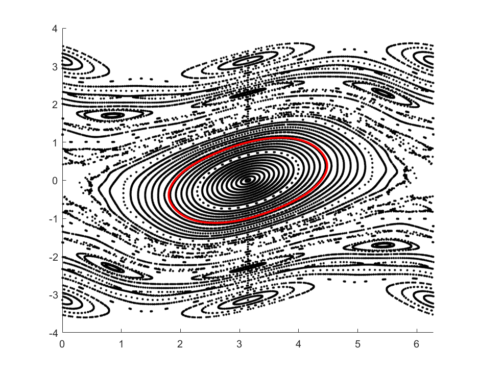
Figure 9: A period 1 quasiperiodic invariant circle for the standard map: phase space simulation and the converged parameterization of a quasiperiodic invariant circle with rotation number $\rho\approx 0.871221766629878$ compute using $50$ Fourier modes.

Taking $\alpha=\pi/2$ and initial points $P=[1.85,0.565]$, and $P=[4.8155,0.5]$, we compute the Fourier parameterizations of period $6$ and period $24$ quasiperiodic systems invariant circles using the ideas described in Section 4.2. These results are illustrated in Figures 10 and 11, and show that the multiple shooting parameterization method works also for non-polynomial nonlinearities.

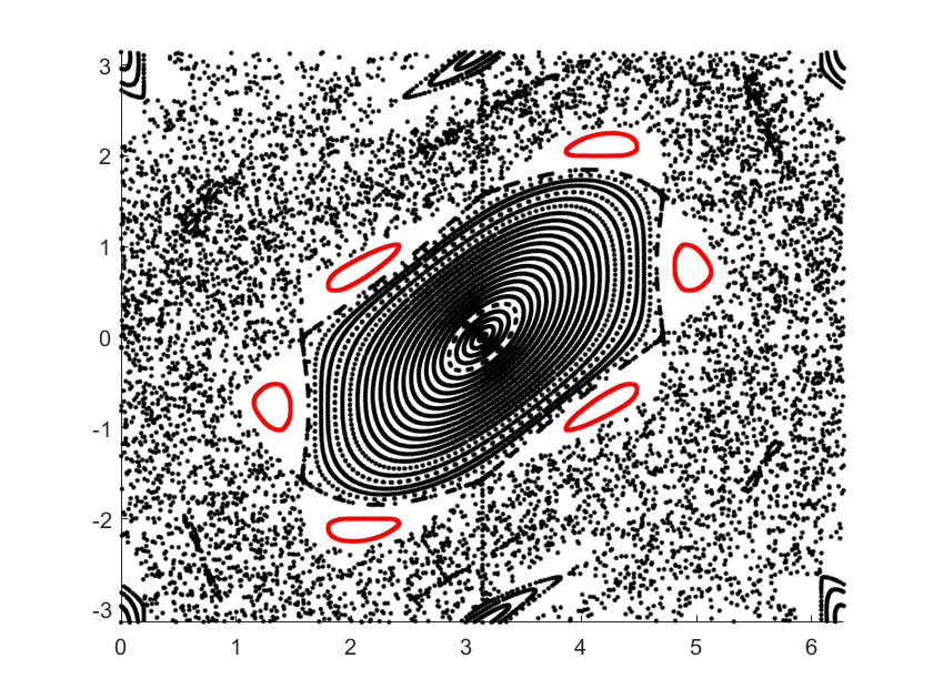
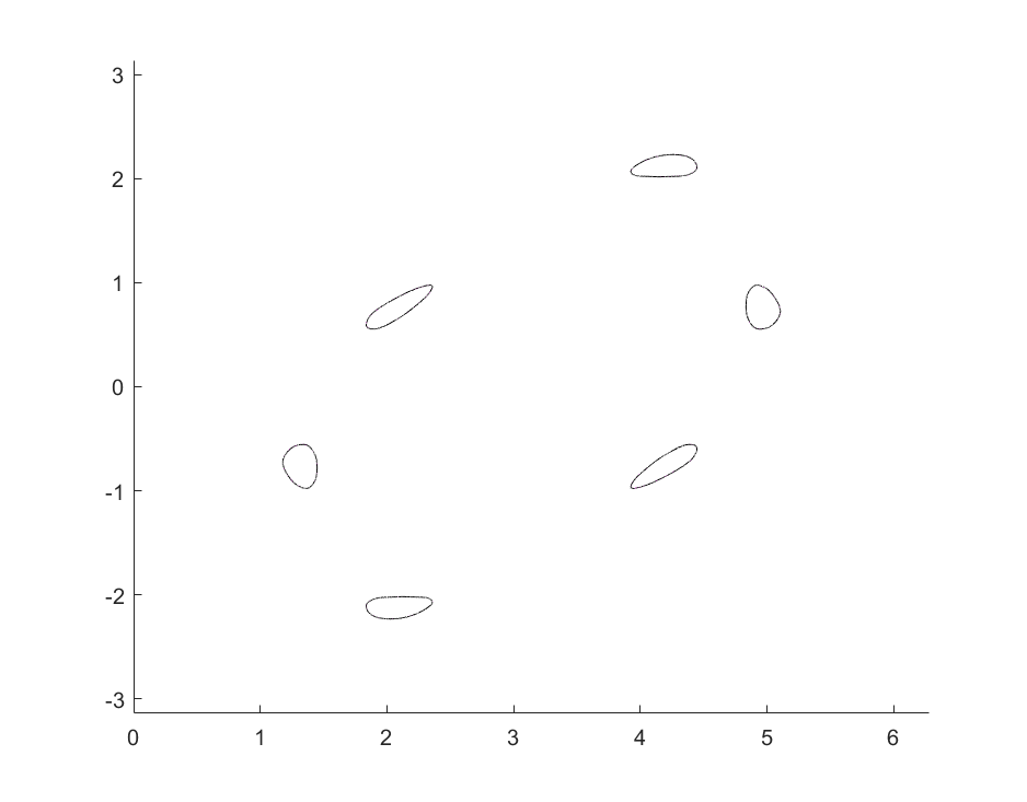
Figure 10: A period 6 quasiperiodic system of invariant circles for the standard map: left figure is a phase space simulation and orbit segment data. Right frame illustrates the image of the converged Fourier approximation.

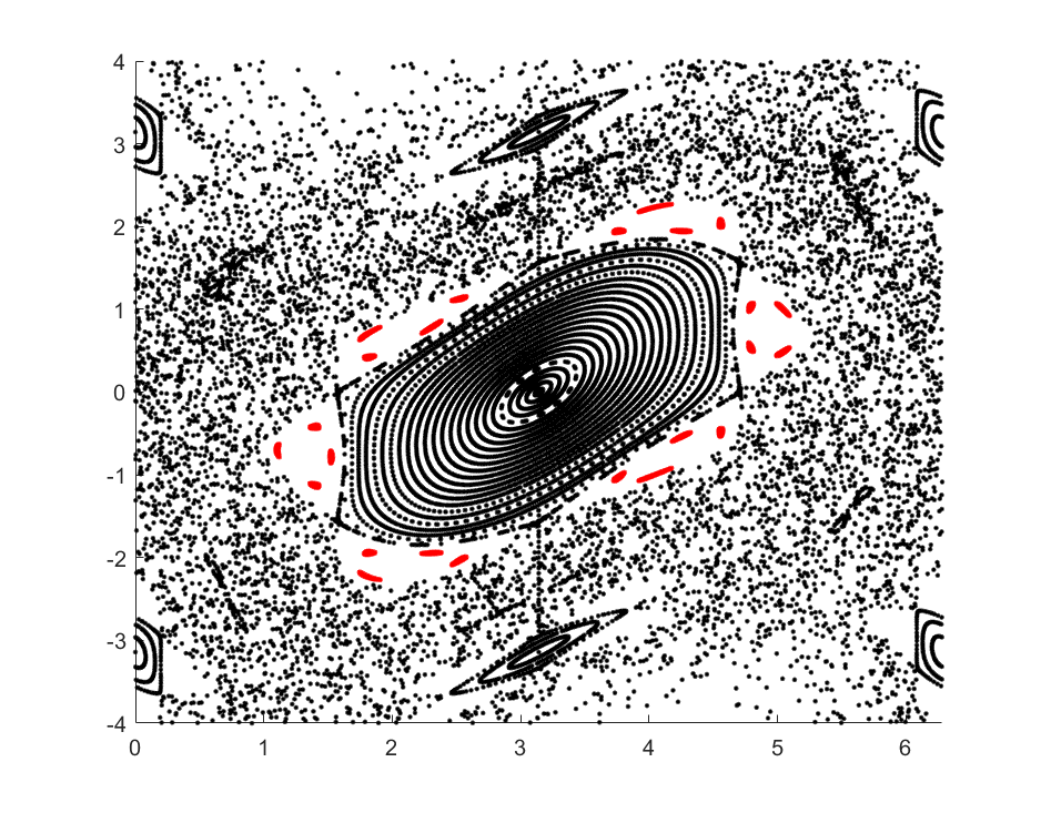
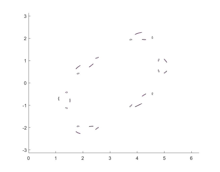
Figure 11: A period 24 quasiperiodic system of invariant circles for the standard map: same left and right as the previous figure.

We cap off this overview of the higher period standard map examples with the observation that the method described produces robust results with small sequence space error. However, the conjugacy error is not so easily controlled, while small, it has so far proved intractable to make arbitrarily so.

4.3.2 Polynomial embedding of non-polynomial nonlinearities

In this section we include a few remarks about the implementation details for the nonlinearity in the standard map. Indeed, suppose that $f$ is a period-$1$ function given by

$$f(\theta)=\sum_{n\in\mathbb{Z}}a_{n}e^{2\pi i\theta},$$

and that we want to compute the Fourier coefficients of the composition

$$\sin(f(\theta))=\sum_{n\in\mathbb{Z}}a_{n}e^{2\pi i\theta}.$$

One approach (perhaps the most natural) is to employ the FFT, and if $f$ is an arbitrary band-limited function and $g$ is smooth, then this in general provides the best known method for computing the Fourier coefficients of $g\circ f$. In the present setting however, the functions being composed have additional structure. They are solutions of certain polynomial functional equations and, by appending these equations to the parameterization method, we obtain a new functional equation whose nonlinearity is only polynomial (in fact quadratic). This avoids the overhead of implementing the FFT, and more importantly overcomes the “numerical stagnation” of the coefficient decay of the composition at 10 or 20 multiples of Machine precision – as is often observed when interpolation based methods for evaluating spectral coefficients are used.

The technique described here is give different names in different communities, for example automatic differentiation [HCF⁺16, LMJR16], polynomial embedding [vdBGL22, H2́1], and quadratic recast [GCV19, CV08] to name only a few. We refer to [BCH⁺06] and also to Chapter 4.7 of [Knu81] for a more thorough discussion of the history of these ideas, going back to the 19th Century. We explain the idea for a period one invariant circle of the standard map.

Consider an invariant circle parameterized by

$$K(\theta)=\left(\begin{array}[]{c}K_{1}(\theta)\\ K_{2}(\theta)\end{array}\right)=\sum_{n\in\mathbb{Z}}\left(\begin{array}[]{c}a_{n}\\ b_{n}\end{array}\right)e^{2\pi i\theta}$$

which passes through the $x$-axis when $\theta=0$. Then an appropriate phase condition is $K_{2}(0)=0$, and we seek a zero of the operator

$$\Psi(a,b,\beta)=\left(\begin{array}[]{c}\sum_{n\in\mathbb{Z}}b_{n}\\ a+b+\alpha S(a)-(1+\beta)R_{\rho}a\\ b+\alpha S(a)-(1+\beta)R_{\rho}b\end{array}\right).$$ (21)

Here $a=\{a_{n}\},b=\{b_{n}\}$ are the Fourier coefficient sequences, $R_{\rho}$ is the diagonal operator defined in coefficient space in Equation (19), and $S$ denotes the map in coefficient space from $a$ to the Fourier coefficients of $\sin(K_{1}(\theta))$. Let $C$ denote the complimentary function which maps the Fourier coefficient sequence $a$ to the Fourier coefficients of the function $\cos(K_{1}(\theta))$.

We write $S=S(K_{1}(\theta))$ and $C=C(K_{1}(\theta))$ to denote the values of $S$ and $C$ at $K_{1}$. Note that $S,C$ have

$$\frac{d}{d\theta}S(K_{1}(\theta))=S^{\prime}(K_{1}(\theta))K_{1}^{\prime}(\theta)=CK_{1}^{\prime}(\theta),$$

and

$$\frac{d}{d\theta}C(K_{1}(\theta))=C^{\prime}(K_{1}(\theta))K_{1}^{\prime}(\theta)=-SK_{1}^{\prime}(\theta),$$

with initial conditions

$$S(0)=\sin\left(\sum_{n\in\mathbb{Z}}a_{n}\right),\quad\quad\mbox{and}\quad\quad C(0)=\cos\left(\sum_{n\in\mathbb{Z}}a_{n}\right).$$

Let $s=\{s_{n}\}$, $c=\{c_{n}\}$ denote the Fourier coefficient sequences of $S$, and $C$, and define the diagonal differentiation operator

$$D(a)_{n}=2\pi ina_{n},\quad\quad\quad n\in\mathbb{Z}.$$

Now suppose that $a,b,c,s,\beta,\gamma,\omega$ is a zero of the operator

$$\Psi(a,b,c,s,\beta,\gamma,\omega)=\left(\begin{array}[]{c}\sum_{n\in\mathbb{Z}}b_{n}\\ \sum_{n\in\mathbb{Z}}s_{n}-\sin\left(\sum_{n\in\mathbb{Z}}a_{n}\right)\\ \sum_{n\in\mathbb{Z}}c_{n}-\cos\left(\sum_{n\in\mathbb{Z}}a_{n}\right)\\ a+b+\alpha s-(1+\beta)R_{\rho}a\\ b+\alpha s-(1+\beta)R_{\rho}b\\ Ds-c*Da-\gamma s+\omega c\\ Dc+c*Da-\gamma c-\omega s\end{array}\right).$$ (22)

It can be shown (using an argument similar to the proof of Lemma 2.3) that $\gamma$ and $\omega$ are unfolding parameters for the differential equations. That is, if the initial conditions are satisfied (i.e. the second and third components of $\Psi$ are zero) and if the sixth and seventh components are zero, then $\gamma=\omega=0$. In this case $s$, $c$ are the Fourier coefficient sequences of $\sin(a),\cos(b)$ respectively. It follows that $a,b,\beta$ solve Equation (21). It then follows from the area preserving property of the standard map that $\beta=0$. Then $a,b$ are the Fourier coefficients of a parameterization of an invariant circle conjugate to irrational rotation $\rho$. We stress that $R_{\rho}$ and $D$ are diagonal linear operators in Fourier space and that $*$ is just the discrete convolution. The operator defined in Equation (22) is then linear except in the last two components where there appear quadratic nonlinearities. This is like a kind of “multiple shooting” for unwrapping compositions, and it is easily extended to the functional equations for periodic systems of invariant circles.

5 Numerical continuation (discrete) for families of periodic invariant circles

While the recipe given in Section 3 is non-perturbative, requiring only finite data sampled form an invariant circle, it is well known (from KAM theory) that quasiperiodic invariant circles for area preserving maps typically appear in Cantor sets of large measure. We refer the reader to any of the classic books/lecture notes of [DlL01, APP90, HK03, Dev03, Rob99], and to their bibliographies for much more complete references. We only note that if $\rho$ is irrational (say Diophantine), then $h\rho$ is irrational (and likely Diophantine) for rational not too small $h$. Suppose now that $\Gamma$ is a quasiperiodic invariant circle with rotation number $\rho$ and that $h$ is a rational number near $1$. Heuristically speaking, it is probable that there exists a nearby quasiperiodic invariant circle $\bar{\Gamma}$ with irrational rotation number $h\rho$.

This suggests that, having found a parameterized invariant circle using the method of Section 3, we perform a kind of (discrete) continuation in the parameter $\rho$. That is, suppose that $\rho_{0}\in[0,1]$ and $K_{0}\colon\mathbb{R}\to\mathbb{R}^{2}$ is one periodic with

$$F(K_{0}(\theta))=K_{0}(\theta+\rho_{0}),\quad\quad\quad\theta\in[0,1].$$

Then we take $\rho_{1}=h\rho_{0}$ (with $h$ close to one) and use $K_{0}$ as the initial condition for a Newton method solving the equation

$$F(K(\theta))=K(\theta+\rho_{1}).$$

The equation just stated is of course solved using the Newton scheme described in Section 2.4.1. Indeed, it is very likely that the new calculation can be performed with exactly the same phase condition. The continuation schemes applies also to period-$K$ systems of quasiperiodic invariant circles.

This kind of discrete continuation (we use the word “discrete” to stress that the family of invariant circles does not vary continuously with $\rho$) has been used many times in the past. Indeed in [CdlL10] the authors show that, for planar symplectic maps, a precursor to “breakdown” or disappearance of a family of KAM tori is the blow-up of certain Sobolev norms associated with the parameterization.

More precisely, a typical invariant circle in the family is actually analytic, so that there is a $\nu>1$ so that

$$\|K\|_{0}=\sum_{n\in\mathbb{Z}}\max(|a_{n}|,|b_{n}|)\nu^{|}n|<\infty.$$

Defining the Sobolev norms

$$\|K\|_{d}^{2}=\sum_{n\in\mathbb{Z}}(1+d^{2})^{|n|}\max(|a_{n}|^{2},|b_{n}|^{2})<\infty,$$

the main result of [CdlL10] can be summarized by saying that if $\Gamma_{\infty}$ is “the last” invariant torus in the Cantor family (the torus at which the family breaks down) then there is a $d$ so that the $d$-th Sobolev norm of the parameterization of $\Gamma_{\infty}$ is infinite. This suggests choosing a $K\in\mathbb{N}$ (perhaps $K=10$) and monitoring the Sobolev norms of the Fourier series coefficients for $1\leq d\leq K$ during the numerical continuation. If one begins to blow up we conclude that we are near the breakdown. This can be used as an automatic stopping procedure for the continuation.

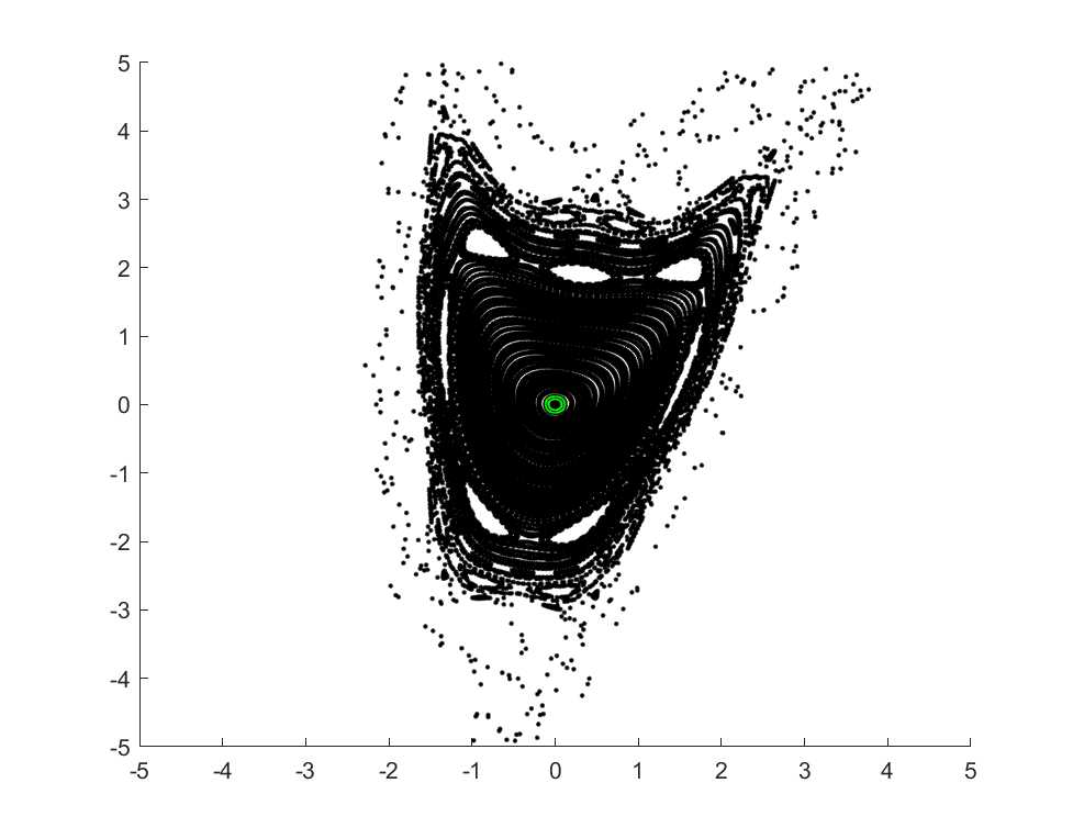
Figure 12: Discrete continuation of a period one family for the area perserving Henon map: in the left frame we see the results of a phase space simulation and the initial small invariant circle. The right frame illustrates the results of the numerical continuation, making it clear that breakdown of the family involves loss of smoothness, as predicted by [CdlL10]. That is, the outermost invariant circles appear to have fairly sharp corners, indicating a blow up in the first Sobolev norm.

Consider for example a small circle, the orbit of $P=[0,0.1]$ in the area preserving Henon maps, and compute the parameterization and the rotation number $\rho\approx 0.550640092644521$. We increment $\rho$ by $0.001$. If the result converges we try again. If not we increase the number of modes, and decrease the increment. In this way we computed 150 invariant circles in the family, and finish with a final increment on the order of $10^{-13}$. At this point the Sobolev norms are large, and we terminate the continuation. The results are illustrated in Figure 12.

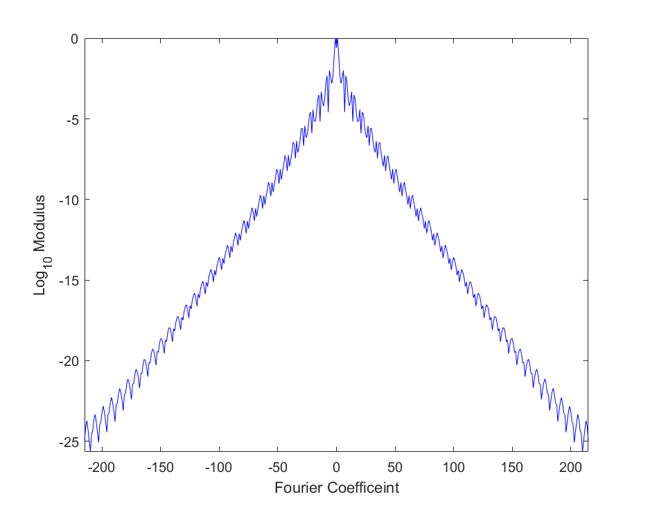
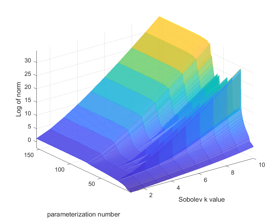
Figure 13: Coefficient decay: The left frame illustrates the decay of the coefficients for the last curve in our continuation computation, and we see that even this circle has quite rapid decay. However the right frame illustrates the Sobolev norms calculated along the entire family, and we see that after about 50 continuation steps they are quite large. We note that for the remaining 100 steps, the step size is very small. That is, most of the progress is made in the first 50 steps.

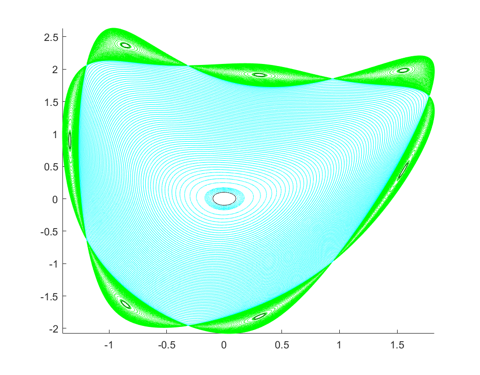
Figure 14: Filling in the phase space: after the period on family we restart the continuation on a period 7 family and continue until breakdown. The union of the results yields a fairly large region of phase space covered by the two Cantor sets.

After the breakdown of the period one family we observe that there appears to be a period 7 family of quasiperiodic circles. We locate the period 7 orbit with a (finite dimensional) Newton scheme, check the elliptic stability type, and look start our search for a period 7 family nearby. Once a single circle is found, we continue again until breakdown. The result os a fairy large set of quasiperiodic motions. The results are illustrated in Figure 14. Continuing in this way, we find – after the original period 1 and period 7 families – a period 1, 19, 1, 55, 1, 12, 120, and 17. These results are illustrated in Figure 15.

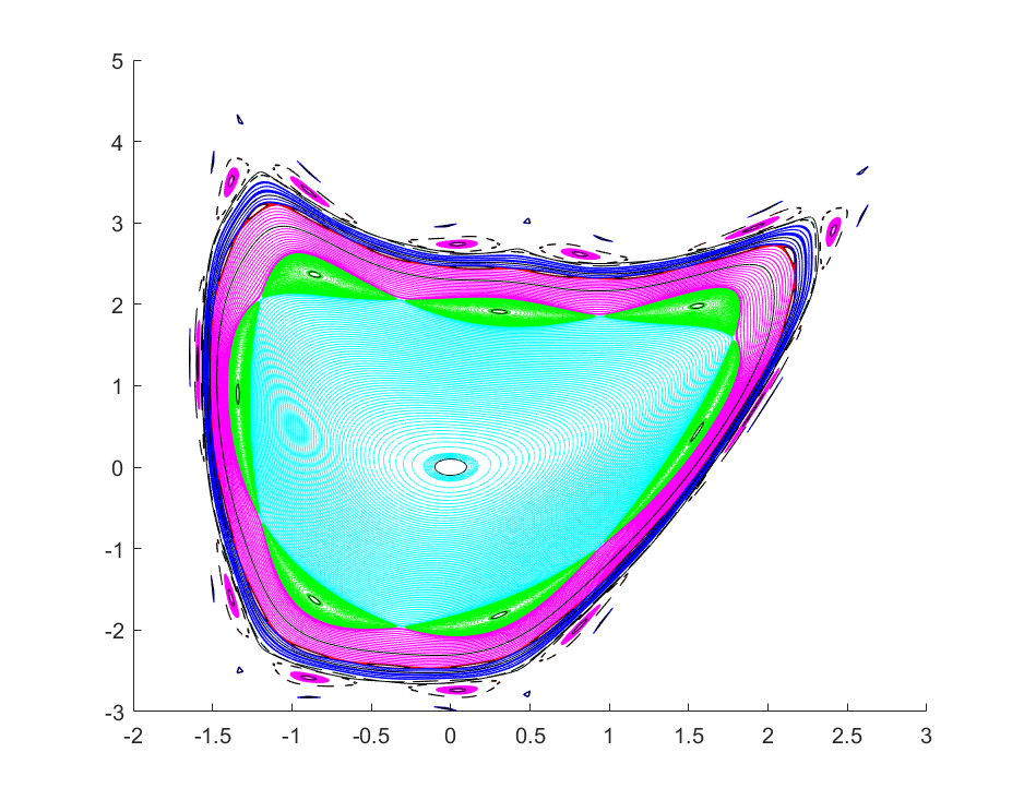
Figure 15: Results of ten different continuations: Note there are no phase space samples in this picture. Only plots of images of Fourier parameterizations. In total – starting from the origin and building out – we see families of period 1 (teal), 7 (green), 1 (magenta), 19 (thin red band), 1 (blue), 55 (thin bands just after blue), 1 (black), 12 (pink), 120 (black spots around the pink family), and 17 (blue). Some of the families are very thin. We do not claim that there are no other tori in this region.

6 Conclusions

The goal of this paper was to demonstrate that the method of weighted Birkhoff averages proves to be the perfect tool for initializing the parameterization method for invariant tori. We have provided detailed example calculations illustrating the approach for classic polynomial and non-polynomial examples. Moreover, we described and implemented a multiple shooting version of the parameterization method for simultaneously computing period-$d$ systems of invariant circles for $d$ as large as 120. We also discuss a quadratic recast/automatic differentiation scheme which reduces the implementation of Newton scheme to diagonal linear operators and discrete convolutions. We also introduced a global unfolding parameter for the parameterization method which is built directly into the nonlinear conjugacy equation. This avoids the need for introducing new parameters in the linear equations at each step of the Newton method. These ideas can be combined with basic numerical schemes to compute large sets of quasiperiodic motions. Taken together, the approach described here provides a flexible general toolkit for computing systems of invariant circles for area preserving maps.

An natural future direction will be to extend the approach taken here for invariant 2-tori in volume preserving maps. For example combining the ergodic averages for 2 tori used in [MS21] with the parameterization method for volume preserving maps developed in [FM16, FdlL15]. We note for example that our unfolding parameter argument extends directly to this case. Extension to invariant tori in higher dimensional symplectic maps should be straight forward, but justifying the unfolding parameter will require considering Calabi invariants. The utility of Calabi invariants in the parameterization method is discussed at length in [HM21]. Another valuable extension is to modify these ideas for application to parameterization of invariant tori for Hamiltonian ODEs, as discussed in [KAdlL22, KAdlL21]. Indeed, the idea of combining rapidly converging Birkhoff averages with Newton schemes for solving invariance equations is so natural it is clear there will be many additional extensions and applications.

7 Acknowledgements

The authors would like to thank Evelyn Sander for illuminating conversations which inspired the present work. In particular, she explained the (then quite recent) results about weighted Birkhoff averages to the second Author during the 2014 AIMS Conference on Dynamical Systems and Applications in Madrid. The author’s also thank Rafael de la Llave for a number of additional helpful discussions. In particular, the idea of using the area preserving property of the dynamical system as a means to formulate an appropriate unfolding parameter for the parameterization method emerged during conversations with the second author during his visit to FAU in 2015. Conversations with Alex Haro, and Jordi-Lluís Figueras are also gratefully acknowledged. The work of the second author was partially supported by NSF grant DMS-1813501 during some of the work on this project.

References

- [APP90] D.K. Arrowsmith, C.M. Place, and C.H. Place. An Introduction to Dynamical Systems. Cambridge University Press, 1990.
- [BCH+06] Martin Bücker, George Corliss, Paul Hovland, Uwe Naumann, and Boyana Norris, editors. Automatic differentiation: applications, theory, and implementations, volume 50 of Lecture Notes in Computational Science and Engineering. Springer-Verlag, Berlin, 2006. Papers from the 4th International Conference on Automatic Differentiation held in Chicago, IL, July 20–24, 2004.
- [CCdlL22] Renato C. Calleja, Alessandra Celletti, and Rafael de la Llave. KAM quasi-periodic solutions for the dissipative standard map. Commun. Nonlinear Sci. Numer. Simul., 106:Paper No. 106111, 29, 2022.
- [CCH21] Renato Calleja, Marta Canadell, and Alex Haro. Non-twist invariant circles in conformally symplectic systems. Commun. Nonlinear Sci. Numer. Simul., 96:Paper No. 105695, 15, 2021.
- [CdlL09] R. Calleja and R. de la Llave. Fast numerical computation of quasi-periodic equilibrium states in 1D statistical mechanics, including twist maps. Nonlinearity, 22(6):1311–1336, 2009.
- [CdlL10] Renato Calleja and Rafael de la Llave. A numerically accessible criterion for the breakdown of quasi-periodic solutions and its rigorous justification. Nonlinearity, 23(9):2029–2058, 2010.
- [CF12] Renato Calleja and Jordi-Lluís Figueras. Collision of invariant bundles of quasi-periodic attractors in the dissipative standard map. Chaos, 22(3):033114, 10, 2012.
- [CFdlL03a] X. Cabré, E. Fontich, and R. de la Llave. The parameterization method for invariant manifolds. I. Manifolds associated to non-resonant subspaces. Indiana Univ. Math. J., 52(2):283–328, 2003.
- [CFdlL03b] X. Cabré, E. Fontich, and R. de la Llave. The parameterization method for invariant manifolds. II. Regularity with respect to parameters. Indiana Univ. Math. J., 52(2):329–360, 2003.
- [CFdlL05] X. Cabré, E. Fontich, and R. de la Llave. The parameterization method for invariant manifolds. III. Overview and applications. J. Differential Equations, 218(2):444–515, 2005.
- [CH17] Marta Canadell and Àlex Haro. Computation of quasi-periodic normally hyperbolic invariant tori: algorithms, numerical explorations and mechanisms of breakdown. J. Nonlinear Sci., 27(6):1829–1868, 2017.
- [Chi79] Boris V. Chirikov. A universal instability of many-dimensional oscillator systems. Phys. Rept., 52:263–379, 1979.
- [CV08] Bruno Cochelin and Christophe Vergez. A high-order, purely frequency based harmonic balance formulation for continuation of periodic solutions: The case of non-polynomial nonlinearities. Journal of Sound and Vibration, 332:968–977, 2008.
- [Dev03] Robert L. Devaney. An introduction to chaotic dynamical systems. Studies in Nonlinearity. Westview Press, Boulder, CO, 2003. Reprint of the second (1989) edition.
- [DlL01] Rafael De la Llave. A tutorial on KAM theory, 01 2001.
- [dlLR90] R. de la Llave and David Rana. Accurate strategies for small divisor problems. Bull. Amer. Math. Soc. (N.S.), 22(1):85–90, 1990.
- [dlLR91] R. de la Llave and D. Rana. Accurate strategies for K.A.M. bounds and their implementation. In Computer aided proofs in analysis (Cincinnati, OH, 1989), volume 28 of IMA Vol. Math. Appl., pages 127–146. Springer, New York, 1991.
- [DSSY16] Suddhasattwa Das, Yoshitaka Saiki, Evelyn Sander, and James A. Yorke. Quasiperiodicity: rotation numbers. In The foundations of chaos revisited: from Poincaré to recent advancements, Underst. Complex Syst., pages 103–118. Springer, [Cham], 2016.
- [DSSY17] Suddhasattwa Das, Yoshitaka Saiki, Evelyn Sander, and James A. Yorke. Quantitative quasiperiodicity. Nonlinearity, 30(11):4111–4140, 2017.
- [DY18] Suddhasattwa Das and James A. Yorke. Super convergence of ergodic averages for quasiperiodic orbits. Nonlinearity, 31(2):491–501, 2018.
- [FdlL15] Adam M. Fox and Rafael de la Llave. Barriers to transport and mixing in volume-preserving maps with nonzero flux. Phys. D, 295/296:1–10, 2015.
- [FH12] Jordi-Lluís Figueras and Àlex Haro. Reliable computation of robust response tori on the verge of breakdown. SIAM J. Appl. Dyn. Syst., 11(2):597–628, 2012.
- [FHL16] Jordi-Lluís Figueras, Alex Haro, and Alejandro Luque. Rigorous computer assisted application of kam theory: a modern approach. (Submitted) arXiv:1601.00084 [math.DS], 2016.
- [FHL17] J.-Ll. Figueras, A. Haro, and A. Luque. Rigorous computer-assisted application of KAM theory: a modern approach. Found. Comput. Math., 17(5):1123–1193, 2017.
- [FM16] Adam M. Fox and James D. Meiss. Computing the conjugacy of invariant tori for volume-preserving maps. SIAM J. Appl. Dyn. Syst., 15(1):557–579, 2016.
- [GCV19] Louis Guillot, Bruno Cochelin, and Christophe Vergez. A generic and efficient Taylor series-based continuation method using a quadratic recast of smooth nonlinear systems. Internat. J. Numer. Methods Engrg., 119(4):261–280, 2019.
- [GHdlL22] Alejandra González, Àlex Haro, and Rafael de la Llave. Efficient and reliable algorithms for the computation of non-twist invariant circles. Found. Comput. Math., 22(3):791–847, 2022.
- [GJMS91] Gerard Gómez, Àngel Jorba, Josep Masdemont, and Carles Simó. Quasiperiodic orbits as a substitute of libration points in the solar system. In Predictability, stability, and chaos in -body dynamical systems (Cortina d’Ampezzo, 1990), volume 272 of NATO Adv. Sci. Inst. Ser. B: Phys., pages 433–438. Plenum, New York, 1991.
- [GMJ17] J. L. Gonzalez and J. D. Mireles James. High-order parameterization of stable/unstable manifolds for long periodic orbits of maps. SIAM J. Appl. Dyn. Syst., 16(3):1748–1795, 2017.
- [H2́1] Olivier Hénot. On polynomial forms of nonlinear functional differential equations. J. Comput. Dyn., 8(3):309–323, 2021.
- [Han69] M. Hanon. Numerical study of quadratic area-preserving mappings. Quarterly of Applied Mathematics, 27(3):291–312, 1969.
- [HCF+16] Àlex Haro, Marta Canadell, Jordi-Lluí s Figueras, Alejandro Luque, and Josep-Maria Mondelo. The parameterization method for invariant manifolds, volume 195 of Applied Mathematical Sciences. Springer, [Cham], 2016. From rigorous results to effective computations.
- [HdlL06a] À. Haro and R. de la Llave. A parameterization method for the computation of invariant tori and their whiskers in quasi-periodic maps: numerical algorithms. Discrete Contin. Dyn. Syst. Ser. B, 6(6):1261–1300 (electronic), 2006.
- [HdlL06b] A. Haro and R. de la Llave. A parameterization method for the computation of invariant tori and their whiskers in quasi-periodic maps: rigorous results. J. Differential Equations, 228(2):530–579, 2006.
- [HdlL07] A. Haro and R. de la Llave. A parameterization method for the computation of invariant tori and their whiskers in quasi-periodic maps: explorations and mechanisms for the breakdown of hyperbolicity. SIAM J. Appl. Dyn. Syst., 6(1):142–207 (electronic), 2007.
- [HK03] Boris Hasselblatt and Anatole Katok. A first course in dynamics. Cambridge University Press, New York, 2003. With a panorama of recent developments.
- [HM21] Alex Haro and J. M. Mondelo. Flow map parameterization methods for invariant tori in Hamiltonian systems. Commun. Nonlinear Sci. Numer. Simul., 101:Paper No. 105859, 34, 2021.
- [HS96] A. Haro and C. Simó. A numerical study of the breakdown of invariant tori in 4D symplectic maps. In XIV CEDYA/IV Congress of Applied Mathematics (Spanish)(Vic, 1995), page 9. Univ. Barcelona, Barcelona, [1996?].
- [Jor01] Àngel Jorba. Numerical computation of the normal behaviour of invariant curves of -dimensional maps. Nonlinearity, 14(5):943–976, 2001.
- [KAdlL21] Bhanu Kumar, Rodney L. Anderson, and Rafael de la Llave. High-order resonant orbit manifold expansions for mission design in the planar circular restricted 3-body problem. Commun. Nonlinear Sci. Numer. Simul., 97:Paper No. 105691, 15, 2021.
- [KAdlL22] Bhanu Kumar, Rodney L. Anderson, and Rafael de la Llave. Rapid and accurate methods for computing whiskered tori and their manifolds in periodically perturbed planar circular restricted 3-body problems. Celestial Mech. Dynam. Astronom., 134(1):Paper No. 3, 38, 2022.
- [KH95] Anatole Katok and Boris Hasselblatt. Introduction to the modern theory of dynamical systems, volume 54 of Encyclopedia of Mathematics and its Applications. Cambridge University Press, Cambridge, 1995. With a supplementary chapter by Katok and Leonardo Mendoza.
- [Knu81] Donald E. Knuth. The art of computer programming. Vol. 2. Addison-Wesley Publishing Co., Reading, Mass., second edition, 1981. Seminumerical algorithms, Addison-Wesley Series in Computer Science and Information Processing.
- [LMJR16] Jean-Philippe Lessard, J. D. Mireles James, and Julian Ransford. Automatic differentiation for Fourier series and the radii polynomial approach. Phys. D, 334:174–186, 2016.
- [MnAFG+03] F. J. Muñoz Almaraz, E. Freire, J. Galán, E. Doedel, and A. Vanderbauwhede. Continuation of periodic orbits in conservative and Hamiltonian systems. Phys. D, 181(1-2):1–38, 2003.
- [MnAGF00] F. J. Muñoz Almaraz, J. Galán, and E. Freire. Numerical continuation of periodic orbits in symmetric Hamiltonian systems. In International Conference on Differential Equations, Vol. 1, 2 (Berlin, 1999), pages 919–921. World Sci. Publ., River Edge, NJ, 2000.
- [MS21] J. D. Meiss and E. Sander. Birkhoff averages and the breakdown of invariant tori in volume-preserving maps. Phys. D, 428:Paper No. 133048, 20, 2021.
- [Rob99] Clark Robinson. Dynamical systems. Studies in Advanced Mathematics. CRC Press, Boca Raton, FL, second edition, 1999. Stability, symbolic dynamics, and chaos.
- [SM20] E. Sander and J. D. Meiss. Birkhoff averages and rotational invariant circles for area-preserving maps. Phys. D, 411:132569, 19, 2020.
- [SVSO06] Frank Schilder, Werner Vogt, Stephan Schreiber, and Hinke M. Osinga. Fourier methods for quasi-periodic oscillations. Internat. J. Numer. Methods Engrg., 67(5):629–671, 2006.
- [TMJ22] Archana Neupane Timsina and J. D. Mireles James. Parameterized stable/unstable manifolds for periodic solutions of implicitly defined dynamical systems. Chaos Solitons Fractals, 161:Paper No. 112345, 20, 2022.
- [vdBGL22] Jan Bouwe van den Berg, Chris Groothedde, and Jean-Philippe Lessard. A general method for computer-assisted proofs of periodic solutions in delay differential problems. J. Dynam. Differential Equations, 34(2):853–896, 2022.