June, 2023

Stability of Electroweak Vacuum and
Supersymmetric Contribution to Muon $g-2$

So Chigusa${}^{(a,b)}$, Takeo Moroi${}^{(c)}$ and Yutaro Shoji${}^{(d)}$

${}^{(a)}$ Berkeley Center for Theoretical Physics, Department of Physics,
University of California, Berkeley, CA 94720, USA

${}^{(b)}$ Theoretical Physics Group, Lawrence Berkeley National Laboratory,
Berkeley, CA 94720, USA

${}^{(c)}$ Department of Physics, The University of Tokyo, Tokyo 113-0033, Japan

${}^{(d)}$ Racah Institute of Physics, Hebrew University of Jerusalem, Jerusalem 91904, Israel

We study the stability of the electroweak vacuum in the supersymmetric (SUSY) standard model (SM), paying particular attention to its relation to the SUSY contribution to the muon anomalous magnetic moment $a_{\mu}$. If the SUSY contribution to $a_{\mu}$ is sizable, the electroweak vacuum may become unstable because of enhanced trilinear scalar interactions in particular when the sleptons are heavy. Consequently, assuming enhanced SUSY contribution to $a_{\mu}$, an upper bound on the slepton masses is obtained. We give a detailed prescription to perform a full one-loop calculation of the decay rate of the electroweak vacuum for the case that the SUSY contribution to $a_{\mu}$ is enhanced. We also give an upper bound on the slepton masses as a function of the SUSY contribution to $a_{\mu}$.

1 Introduction

It has been argued that the electroweak (EW) vacuum, on which we are living, may not be absolutely stable and it can be a false vacuum. For example, even in the standard model (SM) of particle physics, the EW vacuum is known to be metastable [Isidori:2001bm, Degrassi:2012ry, Buttazzo:2013uya, Bednyakov:2015sca, Andreassen:2017rzq, Chigusa:2017dux, Chigusa:2018uuj]. Even though the longevity of the EW vacuum is guaranteed with the observed values of the top-quark mass $m_{t}\simeq$172.69\text{\,}\mathrm{G}\mathrm{e}\mathrm{V}$$ and the Higgs-boson mass $m_{h}\simeq$125.25\text{\,}\mathrm{G}\mathrm{e}\mathrm{V}$$ [ParticleDataGroup:2020ssz], the lifetime of the EW vacuum would have been shorter than the present age of the universe if the top-quark mass were heavier than $\sim 177-178\ {\rm GeV}$. In addition, if we consider physics beyond the standard model (BSM), the stability of the EW vacuum is not guaranteed. This is particularly the case in supersymmetric (SUSY) models, which have attracted attentions as possible solutions to problems that cannot be solved within the SM. In particular, it has been discussed that the SUSY contribution to the muon anomalous magnetic moment $a_{\mu}$ may explain the discrepancy between the experimentally measured value $a_{\mu}^{\rm(exp)}$ and the SM prediction $a_{\mu}^{\rm(SM)}$ (i.e., so-called the muon $g-2$ anomaly). For example, adopting the SM prediction given in Ref. [Aoyama:2020ynm], the deviation between $a_{\mu}^{\rm(exp)}$ and $a_{\mu}^{\rm(SM)}$ is about $4.2\sigma$ (for more detail, see the next section). It has been discussed that the SUSY contribution can be large enough to explain such a deviation (see, for example, [Chakraborti:2021kkr, Endo:2021zal, Han:2021ify, VanBeekveld:2021tgn, Ahmed:2021htr, Cox:2021nbo, Wang:2021bcx, Baum:2021qzx, Yin:2021mls, Iwamoto:2021aaf, Athron:2021iuf, Shafi:2021jcg, Aboubrahim:2021xfi, Chakraborti:2021bmv, Baer:2021aax, Aboubrahim:2021phn, Li:2021pnt, Jeong:2021qey, Ellis:2021zmg, Nakai:2021mha, Forster:2021vyz, Ellis:2021vpp, Chakraborti:2021mbr, Gomez:2022qrb, Chakraborti:2022vds, Agashe:2022uih, Morrison:2022vqe, Li:2022zap, Zhao:2022pnv, He:2023lgi] for recent studies).

In the minimal SUSY SM (MSSM), there is an extra SUSY contribution to the muon anomalous magnetic moment, which can mitigate the muon $g-2$ anomaly. Because the SUSY contribution to the muon $g-2$ is due to the diagrams with superparticles in the loops, it is suppressed as the superparticles become heavier. Thus, in order to explain the muon $g-2$ anomaly, the masses of superparticles are bounded from above. A detailed understanding of the upper bound is important in order to test the SUSY interpretation of the muon $g-2$ anomaly with the on-going and the future collider experiments [Endo:2013lva, Endo:2013xka, Endo:2022qnm, Chigusa:2022xpq]. The muon $g-2$ anomaly can be explained in various parameter regions of the MSSM. If the masses of all the superparticles are comparable, they are required to be of $O(100)\ {\rm GeV}$. Then, the muon $g-2$ anomaly indicates that superparticles (in particular, sleptons, charginos, and neutralinos) are important targets of the on-going and the future collider experiments. The SUSY contribution to the muon $g-2$ can be, however, sizable even if some of the superparticles are much heavier. It happens when the Higgsino mass parameter (i.e., the so-called $\mu$ parameter) is significantly large, which results in the enhanced smuon-smuon-Higgs trilinear scalar coupling.

The enhanced scalar trilinear couplings may cause the EW vacuum instability. In the MSSM, scalar partners of SM fermions (i.e., quarks and leptons) are introduced. As we will discuss in the following sections, the absolute minimum of the scalar potential in the MSSM may be the color- and/or charge-breaking (CCB) minimum at which sfermions acquire non-zero expectation values. When the potential has the CCB absolute minimum, the EW vacuum is a false vacuum and decays into the true vacuum (i.e., CCB one) with a finite lifetime; the model is not viable if the lifetime is shorter than the present age of the Universe. In particular, as the scalar trilinear couplings become larger, the corresponding CCB vacuum tends to have lower potential energy and the EW vacuum becomes less stable [Frere:1983ag, Gunion:1987qv, Casas:1995pd, Kusenko:1996jn]. Thus, requiring that $a_{\mu}^{\rm(SUSY)}$ be large enough to solve (or relax) the muon $g-2$ anomaly, we can obtain upper bounds on the masses of superparticles based on the observed longevity of the EW vacuum.

The stability of the EW vacuum was considered in Ref. [Endo:2021zal] in connection with the muon $g-2$ anomaly. Ref. [Endo:2021zal] estimated the lifetime of the EW vacuum using the tree-level bounce action. (For other studies of the stability of the EW vacuum in the MSSM, see Refs. [Endo:2013lva, Chowdhury:2013dka, Badziak:2014kea, Duan:2018cgb, Hollik:2018wrr, Chigusa:2022xpq]. The tree-level estimation of the decay rate, however, suffers from the uncertainty in determining the normalization factor of the decay rate (i.e., the prefactor $\mathcal{A}$ which will be introduced in Section 4). In order for a reliable estimate of the decay rate, the ab-initio calculation of the prefactor is necessary, which requires a full one-loop calculation of the decay rate. Results of such a calculation were presented in Ref. [Chigusa:2022xpq] by the present authors, leaving the detailed formulas for the calculation to the subsequent publication. In this paper, in the following, we give a detailed prescription to perform such a one-loop calculation, based on the state-of-the-art formula to calculate the decay rate of a false vacuum [Endo:2017gal, Endo:2017tsz, Chigusa:2020jbn].

The aim of this paper is to provide a detailed description of the one-loop calculation of the vacuum decay rate in the MSSM. In this paper, we present explicit formulas based on which the one-loop calculation can be performed. Then, we extend the analysis of Ref. [Chigusa:2022xpq] and derive an upper bound on the smuon mass as a function of the SUSY contribution to the muon anomalous magnetic moment. We also study the case where three flavors of the sleptons and the Bino are relatively light, while all the other superparticles are decoupled.

This paper is organized as follows. In Section 2, we overview the SUSY contribution to the muon anomalous magnetic moment. In Section 3, we define low-energy effective field theories (EFTs), which are obtained by integrating out heavy superparticles irrelevant to our discussion. The EFTs introduced in Section 3 are used for the calculation of the decay rate. In Section 4, we present the prescription to perform the one-loop calculation of the decay rate, taking into account the effects of SUSY particles relevant for the muon $g-2$ anomaly. In Section 5, we discuss phenomenological implications of the EW vacuum stability by numerically evaluating the decay rate of the EW vacuum. Section 6 is devoted to the conclusion and discussions.

2 Muon $g-2$: SM and SUSY Contributions

In this section, we first summarize the SM prediction of $a_{\mu}$ as well as the experimentally measured value. Then, we give a brief overview of the SUSY contributions.

2.1 SM prediction

The muon anomalous magnetic moment has been measured with very high accuracy. Combining the results of BNL and FermiLab experiments, the experimentally measured value of the muon anomalous magnetic moment $a_{\mu}$ is given by [Bennett:2002jb, Bennett:2004pv, Bennett:2006fi, Abi:2021gix]

$$a_{\mu}^{\rm(exp)}=(11\,659\,206.1\pm 4.1)\times 10^{-10}.$$ (2.1)

Significant efforts have been made to understand the theoretical prediction of the muon anomalous magnetic moment. In particular, in the SM, a very precise calculation of $a_{\mu}$ has been performed. One important quantity necessary to obtain the theoretical prediction is the hadronic vacuum polarization (HVP) of photon. The effect of the HVP has been estimated by using the so-called $R$-ratio from the data provided by $e^{+}e^{-}$ collider experiments; combining the HVP contribution based on the $R$-ratio with other contributions, Ref. [Aoyama:2020ynm] obtained the SM prediction as

$$a_{\mu}^{\rm(SM)}=(11\,659\,181.0\pm 4.3)\times 10^{-10}.$$ (2.2)

We adopt the above result as our canonical value of the SM prediction.

Comparing Eqs. (2.1) and (2.2), the experimentally measured value is about $4.2\sigma$ away from the SM prediction:

$$a_{\mu}^{\rm(exp)}-a_{\mu}^{\rm(SM)}=(25.1\pm 5.9)\times 10^{-10}.$$ (2.3)

The deviation is sometimes called the muon $g-2$ anomaly. For later convenience, we define the “$0\sigma$,” “$1\sigma$,” and “$2\sigma$” values of BSM contribution to $a_{\mu}$ necessary to resolve the discrepancy:

$$\Delta a_{\mu}^{(0\sigma)}=25.1\times 10^{-10},$$ (2.4)

$$\Delta a_{\mu}^{(1\sigma)}=19.2\times 10^{-10},$$ (2.5)

$$\Delta a_{\mu}^{(2\sigma)}=13.3\times 10^{-10}.$$ (2.6)

Besides, the HVP has been also estimated by using lattice Monte Carlo simulation. The BMW collaboration reached the sub-percent precision in calculating the leading-order HVP to $a_{\mu}$ [Borsanyi:2020mff], based on which the tension between the experimentally measured value and the SM prediction is significantly weakened. Other recent results of lattice calculations are consistent with the BMW result, particularly for the so-called “intermediate time window observable” [Wang:2022lkq, Ce:2022kxy, ExtendedTwistedMass:2022jpw, Bazavov:2023has, Blum:2023qou]. Adopting the BMW result for the estimation of the HVP contribution, $a_{\mu}^{\rm(exp)}-a_{\mu}^{\rm(SM,BMW)}=(10.7\pm 7.0)\times 10^{-10}$ (with $a_{\mu}^{\rm(SM,BMW)}$ being the SM prediction based on the BMW result), meaning that the consistency between $a_{\mu}^{\rm(exp)}$ and $a_{\mu}^{\rm(SM,BMW)}$ is $1.5\sigma$ [latticeave2023]. In addition, a new measurement of the cross section of the process $e^{+}e^{-}\rightarrow\pi^{+}\pi^{-}$ has been performed in the center of mass energy range from $0.32$ to $1.2\ {\rm GeV}$ using the CMD-3 detector at the $e^{+}e^{-}$ collider VEPP-2000 [CMD-3:2023alj]; its result indicates $\sim 3\ \%$ increase of the $\pi^{+}\pi^{-}$ contribution to the HVP contribution to $a_{\mu}$ compared to the one before the CMD-3 result. If one uses the value given in Ref. [CMD-3:2023alj], the tension between the theoretical prediction and the experimentally measured value of $a_{\mu}$ reduces to $\sim 2.3\ \sigma$. Currently, it is still premature to conclude which value of the SM prediction of $a_{\mu}$ is the most reliable. In this paper, we take Eq. (2.3) seriously and regard the discrepancy as a hint of the BSM physics, although we will also comment on the implications of the lattice results of the HVP contribution on the stability of the EW vacuum in the MSSM.

2.2 Supersymmetric contribution to muon $g-2$

As discussed in the previous subsection, the experimentally measured value of the muon anomalous magnetic moment may be in tension with the SM prediction. The discrepancy may suggest the existence of BSM physics that affects $a_{\mu}$. SUSY is one of such possibilities and, in the following, we assume that it is the case. Below, we overview the SUSY contribution to the muon $g-2$ in the MSSM. We also explain why the stability of the EW vacuum is important in the study of the SUSY contribution.

It is well known that the SUSY contribution to the muon anomalous magnetic moment, which is denoted as $a_{\mu}^{\rm(SUSY)}$, is enhanced when $\tan\beta$ is large. Here $\tan\beta$ is the ratio of the two Higgs bosons (denoted as $H_{u}$ and $H_{d}$, respectively). We concentrate on the large $\tan\beta$ case so that the requirement on the mass scale of the smuons to solve the muon $g-2$ anomaly is expected to become higher. Notice that $\tan\beta$ cannot be arbitrarily large if we require the perturbativity of the coupling constants. In particular, because the grand unified theory (GUT) is one of the strong motivations to consider the MSSM, we require that the coupling constants (in particular, the bottom Yukawa coupling constant) are perturbative up to the GUT scale. Then, $\tan\beta$ should be smaller than $\sim 50-60$.

In order to study the behavior of $a_{\mu}^{\rm(SUSY)}$ in the large $\tan\beta$ case, it is instructive to use the so-called mass insertion approximation in which $a_{\mu}^{\rm(SUSY)}$ is estimated in the gauge-eigenstate basis with treating the interactions proportional to the VEVs of the Higgs bosons as perturbations. (In our following numerical calculation, however, $a_{\mu}^{\rm(SUSY)}$ is estimated more precisely using the mass eigenstates of the sleptons, charginos, and neutralinos, as we will explain.) Because the superparticles are in the loop, $a_{\mu}^{\rm(SUSY)}$ is suppressed as the superparticles become heavier. For the case where the masses of all the superparticles are comparable, for example, the SUSY contribution to the muon anomalous magnetic moment is approximately given by $|a_{\mu}^{\rm(SUSY)}|\simeq\frac{5g_{2}^{2}}{192\pi^{2}}\frac{m_{\mu}^{2}}{m_{\rm SUSY}^{2}}\tan\beta$, where $g_{2}$ is the gauge coupling constant of $SU(2)_{L}$ and $m_{\rm SUSY}^{2}$ is the mass scale of superparticles. (Here, the contributions of the diagrams containing the Bino are neglected because they are subdominant.) Taking $\tan\beta\sim 50$, the superparticles should be lighter than $\sim 700\ {\rm GeV}$ in order to make the total muon anomalous magnetic moment consistent with the observed value at the $2\sigma$ level.

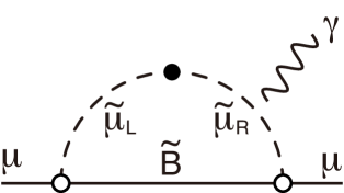
Figure 1: Bino-Smuon diagram of the SUSY contribution to the muon anomalous magnetic moment. The mass insertion approximation is adopted. The black blob is the two-point interaction induced by the VEVs of the Higgs bosons.

Such an upper bound is significantly altered by the Bino-smuon diagram (see Fig. 1). The other $\tan\beta$-enhanced diagrams have slepton, gaugino, and Higgsino propagators in the loop and hence contributions of them are suppressed when any of the sleptons, gauginos, or Higgsinos are heavy. On the contrary, the Bino-smuon diagram has only the smuon and Bino propagators in the loop, and its contribution is approximately proportional to the Higgsino mass parameter, $\mu$. Thus, in the parameter region with a very large $\mu$ parameter, the contribution of the Bino-smuon diagram can be large enough to cure the muon $g-2$ anomaly even if some of the superparticles (in particular, Higgsinos) are much heavier than the upper bound estimated above.

In the following, we study the upper bound on the masses of superparticles in the light of the muon $g-2$ anomaly, paying particular attention to the contribution of the Bino-smuon diagram. In a parameter region where the Bino-smuon diagram dominates $a_{\mu}^{\rm(SUSY)}$, the $\mu$ parameter is large and hence the smuon-smuon-Higgs trilinear coupling is enhanced. A large trilinear scalar coupling is, in general, dangerous because it may make the EW vacuum unstable. In the present case, a large smuon-smuon-Higgs trilinear coupling develops another deeper vacuum, with which the EW vacuum becomes a false vacuum. Consequently, the lifetime of the EW vacuum may become shorter than the present cosmic age [ParticleDataGroup:2020ssz]:

$$t_{\rm now}\simeq 13.8\ {\rm Gyr}.$$ (2.7)

In addition, a large $\mu$ parameter generally enhances all the slepton-slepton-Higgs trilinear couplings. When the stau is light, it is important to study the instability due to the stau-stau-Higgs trilinear coupling since it typically gives a more stringent constraint than the smuon-smuon-Higgs trilinear coupling.

3 Effective Field Theory Analysis

3.1 MSSM

Our main purpose is to calculate the decay rate of the EW vacuum, taking into account the effects of SUSY particles. In particular, we are interested in the upper bound on the masses of superparticles under the requirement that the muon $g-2$ anomaly be solved (or relaxed) by the SUSY contribution. We are interested in the case where the $\mu$ parameter is large so that the Bino-smuon diagram dominates $a_{\mu}^{\rm(SUSY)}$; hereafter, we focus on the case of $\mu\gtrsim O(10)\ {\rm TeV}$. In such a case, $a_{\mu}^{\rm(SUSY)}$ can be large enough to solve the muon $g-2$ anomaly even with relatively large smuon and Bino masses.

A large value of $\mu$ implies heavy Higgsinos. In addition, in order to push the lightest Higgs mass up to the observed value, i.e., about $125\ {\rm GeV}$ [ATLAS:2015yey, ATLAS:2018tdk, CMS:2020xrn], relatively heavy stop masses are preferred [Bagnaschi:2014rsa], which are characterized by a scale $M_{S}$. On the contrary, in order to enhance $a_{\mu}^{\rm(SUSY)}$, smuon and Bino masses should be close to the EW scale. Based on these considerations, in this paper, we consider two cases where the Bino, denoted by $\tilde{B}$, and either only the second generation of sleptons or all three generations of sleptons are relatively light among the MSSM particles. The other MSSM constituents are assumed to have masses of $O(M_{S})$. Here, we assume that Wino and gluino masses are of $O(M_{S})$ just for simplicity. We also assume that there exists a large hierarchy between the EW scale and $M_{S}$.

A large value of $\mu$ suggests relatively large values of the soft SUSY breaking Higgs mass parameters for a viable EW symmetry breaking; the lighter Higgs mass, i.e., the mass of the SM-like Higgs boson $H$, is realized by the cancellation between the contributions of the $\mu$ and soft SUSY breaking parameters. The heavier Higgs bosons are expected to have masses of $O(M_{S})$, comparable to $\mu$. In such a case, the SM-like Higgs $H$ and the heavy doublet $H^{\prime}$ are given by linear combinations of the up- and down-type Higgs bosons as

$$\left(\begin{array}[]{c}H\\ H^{\prime}\end{array}\right)=\left(\begin{array}[]{cc}\cos\beta&\sin\beta\\ -\sin\beta&\cos\beta\end{array}\right)\left(\begin{array}[]{c}H_{d}^{*}\\ H_{u}\end{array}\right).$$ (3.7)

In summary, we are interested in the case where the mass spectrum below $\sim$ TeV scale includes one or three sleptons and the Bino $\tilde{B}$, as well as the SM particles. Hereafter, the leptons (sleptons) in the $\alpha$-th generation in the gauge eigenstate are denoted as $\ell_{L\alpha}$ and $\ell_{R\alpha}$ ($\tilde{\ell}_{L\alpha}$ and $\tilde{\ell}_{R\alpha}$); $\ell_{L\alpha}$ and $\tilde{\ell}_{L\alpha}$ are $SU(2)_{L}$ doublets with hypercharge $-\frac{1}{2}$, while $\ell_{R\alpha}$ and $\tilde{\ell}_{R\alpha}$ are $SU(2)_{L}$ singlets with hypercharge $+1$. For the calculation of the muon $g-2$, sleptons in the second generation are important; they are also denoted as

$$\tilde{\ell}_{L2}=\begin{pmatrix}\tilde{\nu}_{\mu}\\ \tilde{\mu}_{L}\end{pmatrix},~{}~{}~{}\tilde{\ell}_{R2}=\tilde{\mu}_{R}.$$ (3.8)

3.2 EFT

We consider the case where there exists a hierarchy between the masses of MSSM particles. To properly evaluate the coupling constants in such a case, we resort to the EFT approach; we use the renormalization group (RG) analysis to evaluate the EFT parameters at the EW scale.

We adopt the top-quark pole mass $M_{t}$ and $M_{S}$ as matching scales of different EFTs. For the renormalization scale $Q<M_{t}$, we consider the QCD+QED that contains the SM gauge couplings and fermion masses as parameters. For $M_{t}<Q<M_{S}$, we adopt the EFT containing the Bino and the sleptons in addition to all the SM particles, which we call the slepton EFT (see below). At $Q=M_{S}$, the slepton EFT is matched to the MSSM. This matching is necessary to relate scalar couplings in the slepton EFT to gauge and Yukawa couplings. We define $M_{S}$ through the following procedure. At $Q=M_{t}$, we give a tree-level estimation of couplings through the relations described below, with which we estimate the Higgsino mass so that the required size of the muon $g-2$ can be obtained from the MSSM contribution. We use this estimate of the Higgsino mass as $M_{S}$.

To specify the model parameters relevant to the calculation of the decay rate of the EW vacuum, we show the Lagrangian of the slepton EFT, which is obtained by integrating out the heavy MSSM particles. In the following, for simplicity, we assume that the effects of CP and flavor violations are negligible. Then, the EFT Lagrangian is given by

$$\mathcal{L}=\mathcal{L}_{\mathrm{kin}}^{(\mathrm{SM})}+\Delta\mathcal{L}_{\mathrm{kin}}+\Delta\mathcal{L}_{\mathrm{Yukawa}}-V,$$ (3.9)

where $\mathcal{L}_{\mathrm{kin}}^{(\mathrm{SM})}$ is the kinetic terms of the SM fields (including the gauge interactions), while $\mathcal{L}_{\mathrm{Yukawa}}^{(\mathrm{SM})}$ represents the SM-like Yukawa interactions. The latter includes the lepton Yukawa interactions as

$$\mathcal{L}_{\mathrm{Yukawa}}^{\mathrm{(SM)}}\ni Y_{\ell\alpha}\ell_{L\alpha}^{\dagger}H\ell_{R\alpha}+\mathrm{h.c.},$$ (3.10)

where $\alpha$ is the flavor index and the sum over the flavor indices is implicit. The additional kinetic terms and Yukawa couplings are described by

$$\Delta\mathcal{L}_{\mathrm{kin}} =|D_{\mu}\tilde{\ell}_{L\alpha}|^{2}+|D_{\mu}\tilde{\ell}_{R\alpha}|^{2}-i\tilde{B}\sigma^{\mu}\partial_{\mu}\tilde{B}^{\dagger}-\left(\frac{1}{2}M_{1}\tilde{B}\tilde{B}+\mathrm{h.c.}\right),$$ (3.11)

$$\Delta\mathcal{L}_{\mathrm{Yukawa}} =Y_{R\alpha}\tilde{\ell}_{R\alpha}^{\dagger}\ell_{R\alpha}\tilde{B}^{\dagger}+Y_{L\alpha}\tilde{\ell}_{L\alpha}^{\dagger}\ell_{L\alpha}\tilde{B}+\mathrm{h.c.},$$ (3.12)

where $D_{\mu}$ denotes the covariant derivative. The scalar potential $V$ is given by

$$V= \,V_{2}+V_{3}+V_{4},$$ (3.13)

where

$$V_{2}= \,m_{H}^{2}|H|^{2}+m_{R\alpha}^{2}\,|\tilde{\ell}_{R\alpha}|^{2}+m_{L\alpha}^{2}\,|\tilde{\ell}_{L\alpha}|^{2},$$ (3.14)

$$V_{3}= \,-T_{\alpha}\tilde{\ell}_{R\alpha}^{*}H^{\dagger}\tilde{\ell}_{L\alpha}+\text{h.c.},$$ (3.15)

$$V_{4}= \,\lambda_{H}|H|^{4}+\lambda_{HR\alpha}|H|^{2}|\tilde{\ell}_{R\alpha}|^{2}+\lambda_{HL\alpha}|H|^{2}|\tilde{\ell}_{L\alpha}|^{2}+\kappa_{\alpha}(H^{\dagger}\tilde{\ell}_{L\alpha})(\tilde{\ell}_{L\alpha}^{\dagger}H)$$

$$+\lambda_{R\alpha\beta}|\tilde{\ell}_{R\alpha}|^{2}|\tilde{\ell}_{R\beta}|^{2}+\lambda_{L\alpha\beta}|\tilde{\ell}_{L\alpha}|^{2}|\tilde{\ell}_{L\beta}|^{2}+\lambda^{\prime}_{L\alpha\beta}|\tilde{\ell}_{L\alpha}^{\dagger}\tilde{\ell}_{L\beta}|^{2}+\lambda_{LR\alpha\beta}|\tilde{\ell}_{R\alpha}|^{2}|\tilde{\ell}_{L\beta}|^{2}.$$ (3.16)

Note that there are some redundancies in the choice of the coupling constants. To resolve these redundancies, we work under the convention that $\lambda_{R\alpha\beta}=\lambda_{R\beta\alpha}$, $\lambda_{L\alpha\beta}=\lambda_{L\beta\alpha}$, $\lambda^{\prime}_{L\alpha\beta}=\lambda^{\prime}_{L\beta\alpha}$, and $\lambda^{\prime}_{L\alpha\alpha}=0$. The first flavor index of $\lambda_{LR\alpha\beta}$ is for the right-handed sleptons and the second one is for the left-handed sleptons. For the sake of the following discussion, we also define

$$\kappa^{\prime}_{\alpha}\equiv\kappa_{\alpha}+\lambda_{HL\alpha}.$$ (3.17)

Coupling constants in different EFTs are related to each other through the matching conditions at the threshold scales. All the SM parameters including the Higgs quartic coupling $\lambda_{H}^{\mathrm{(SM)}}$ and the mass $m_{H}^{2\mathrm{(SM)}}$ are determined at the energy scale $M_{t}$ and below. Some of the couplings such as the top Yukawa coupling, gauge couplings, $\lambda_{H}^{\mathrm{(SM)}}$, and $m_{H}^{2\mathrm{(SM)}}$ are significantly affected by the weak-scale threshold corrections. We use the results of Ref. [Buttazzo:2013uya] to fix these parameters with using physical parameters $\alpha_{3}(M_{Z})=0.1179$, $M_{t}=172.76\,\mathrm{GeV}$, $M_{W}=80.379\,\mathrm{GeV}$, and $M_{h}=125.25\,\mathrm{GeV}$ [ParticleDataGroup:2020ssz] as inputs. As for the light fermion couplings, we calculate the running of their masses with the one-loop QED and the three-loop QCD beta functions [Gorishnii:1990zu, Tarasov:1980au, Gorishnii:1983zi] to determine the corresponding Yukawa couplings at $Q=M_{t}$.

We perform the matching between the SM and the slepton EFT at $Q=M_{t}$ taking into account important one-loop corrections. For the Higgs quartic coupling and the mass term, we adopt

$$\lambda_{H}^{\mathrm{(SM)}} =\lambda_{H}-\Delta\lambda_{H},$$ (3.18)

$$m_{H}^{2\mathrm{(SM)}} =m_{H}^{2}-\Delta m_{H}^{2},$$ (3.19)

with

$$(16\pi)^{2}\Delta\lambda_{H}= \left(\lambda_{HL\alpha}^{2}+\frac{1}{2}{\kappa^{\prime}_{\alpha}}^{2}+\lambda_{HL\alpha}\kappa^{\prime}_{\alpha}\right)B_{0}(m_{L\alpha}^{2},m_{L\alpha}^{2})+\frac{1}{2}\lambda_{HR\alpha}^{2}B_{0}(m_{R\alpha}^{2},m_{R\alpha}^{2})$$

$$+\lambda_{HL\alpha}T_{\alpha}^{2}C_{0}(m_{L\alpha}^{2},m_{L\alpha}^{2},m_{R\alpha}^{2})+\lambda_{HR\alpha}T_{\alpha}^{2}C_{0}(m_{R\alpha}^{2},m_{R\alpha}^{2},m_{L\alpha}^{2})$$

$$+\frac{1}{2}T_{\alpha}^{4}D_{0}(m_{L\alpha}^{2},m_{R\alpha}^{2},m_{L\alpha}^{2},m_{R\alpha}^{2}),$$ (3.20)

$$(16\pi)^{2}\Delta m_{H}^{2}= \left(2\lambda_{HL\alpha}+\kappa^{\prime}_{\alpha}\right)A_{0}(m_{L\alpha}^{2})+\lambda_{HR\alpha}A_{0}(m_{R\alpha}^{2})+T_{\alpha}^{2}B_{0}(m_{L\alpha}^{2},m_{R\alpha}^{2}),$$ (3.21)

where $A_{0}$, $B_{0}$, $C_{0}$, and $D_{0}$ are the Passarino-Veltman one-, two-, three-, and four-point functions without momentum inflow [Passarino:1978jh], respectively. We also take account of the one-loop corrections to the lepton Yukawa couplings because it can significantly affect the decay rate of the EW vacuum. The one-loop correction to the lepton Yukawa matrix $\Delta Y_{\ell}$, with which the EFT Yukawa matrix $Y_{\ell}$ is related to the SM one $Y_{\ell}^{\mathrm{(SM)}}$ as $Y_{\ell}^{\mathrm{(SM)}}=Y_{\ell}-\Delta Y_{\ell}$, is given by

$$(16\pi)^{2}\Delta Y_{\ell\alpha}=Y_{R\alpha}T_{\alpha}Y_{L\alpha}M_{1}J(M_{1}^{2},m_{R\alpha}^{2},m_{L\alpha}^{2}),$$ (3.22)

with

$$J(a,b,c)\equiv-\frac{ab\ln(a/b)+bc\ln(b/c)+ca\ln(c/a)}{(a-b)(b-c)(c-a)}.$$ (3.23)

These corrections can be sizable because of the hierarchy between $M_{t}$ and $M_{S}$.

Some of the parameters in the slepton EFT are related to each other due to the SUSY relation among coupling constants. Thus, we should impose the matching conditions on the couplings at the matching scale $Q=M_{S}$. At the tree-level, these conditions are given by

$$Y_{L\alpha} =\sqrt{\frac{3}{10}}g_{1},$$ (3.24)

$$Y_{R\alpha} =-\sqrt{\frac{6}{5}}g_{1},$$ (3.25)

for the slepton Yukawa couplings, and

$$\lambda_{R\alpha\beta} =\frac{3}{10}g_{1}^{2},$$ (3.26)

$$\lambda_{L\alpha\beta} =\frac{1}{8}g_{2}^{2}(2\delta_{\alpha\beta}-1)+\frac{3}{40}g_{1}^{2},$$ (3.27)

$$\lambda^{\prime}_{L\alpha\beta} =\frac{1}{4}g_{2}^{2}(1-\delta_{\alpha\beta})$$ (3.28)

$$\lambda_{LR\alpha\beta} =\frac{|Y_{\ell\alpha}|^{2}}{\cos^{2}\beta}\delta_{\alpha\beta}-\frac{3}{10}g_{1}^{2},$$ (3.29)

$$\lambda_{HR\alpha} =|Y_{\ell\alpha}|^{2}-\frac{3}{10}g_{1}^{2}\cos 2\beta,$$ (3.30)

$$\lambda_{HL\alpha} =\left(\frac{1}{4}g_{2}^{2}+\frac{3}{20}g_{1}^{2}\right)\cos 2\beta,$$ (3.31)

$$\kappa^{\prime}_{\alpha} =|Y_{\ell\alpha}|^{2}-\left(\frac{1}{4}g_{2}^{2}-\frac{3}{20}g_{1}^{2}\right)\cos 2\beta,$$ (3.32)

$$T_{\alpha} =Y_{\ell\alpha}\mu\tan\beta,$$ (3.33)

for the scalar quartic and trilinear couplings, where $g_{2}$ and $g_{1}$ are the gauge couplings of $SU(2)_{L}$ and $U(1)_{Y}$, respectively. (Here we use the $SU(5)$ normalization of the $U(1)_{Y}$ coupling $g_{1}^{2}\equiv 5g_{Y}^{2}/3$.) We neglect SUSY breaking trilinear scalar interactions for simplicity. We also neglect the threshold corrections to the above matching conditions due to the MSSM particles as heavy as $\sim M_{S}$, because such corrections depend on the detailed mass spectrum of heavy particles.

Although we determine $\lambda_{H}$ at $Q=M_{t}$, there is also a SUSY relation between $\lambda_{H}$ and other couplings. Considering only the stop contribution to the threshold correction, which is in many cases the largest, we obtain the one-loop matching condition [Bagnaschi:2014rsa]

$$\lambda_{H}=\left[\frac{1}{8}g_{2}^{2}+\frac{3}{40}g_{1}^{2}\right]\cos^{2}2\beta+\delta\lambda_{H},$$ (3.34)

with

$$(16\pi^{2})\delta\lambda_{H}\simeq \,\frac{3}{2}y_{t}^{2}\left[y_{t}^{2}+\left(\frac{1}{2}g_{2}^{2}-\frac{1}{10}g_{1}^{2}\right)\cos 2\beta\right]\ln\frac{m_{Q3}^{2}}{Q^{2}}$$

$$+\frac{3}{2}y_{t}^{2}\left[y_{t}^{2}+\frac{2}{5}g_{1}^{2}\cos 2\beta\right]\ln\frac{m_{U3}^{2}}{Q^{2}}$$

$$+\frac{\cos^{2}2\beta}{200}\left[(25g_{2}^{4}+g_{1}^{4})\ln\frac{m_{Q3}^{2}}{Q^{2}}+8g_{1}^{4}\ln\frac{m_{U3}^{2}}{Q^{2}}+2g_{1}^{4}\ln\frac{m_{D3}^{2}}{Q^{2}}\right],$$ (3.35)

where $y_{t}$ is the top Yukawa coupling, and $m_{Q3}$, $m_{U3}$, and $m_{D3}$ the mass parameters of the third generation left-handed squark, right-handed up-type squark, and right-handed down-type squark, respectively. Once the value of $\lambda_{H}$ at the matching scale $Q=M_{S}$ is obtained, we can solve (3.34) against the stop mass $m_{\tilde{t}}$ assuming the universality $m_{\tilde{t}}\equiv m_{Q3}=m_{U3}=m_{D3}$. It is known that a sizable threshold correction is needed to realize the observed value $M_{h}=125.25\,\mathrm{GeV}$. In the present case, we checked that, with a moderate choice of $m_{\tilde{t}}\lesssim 100\,\mathrm{TeV}$ (and thus $m_{\tilde{t}}\sim\mu$), the observed Higgs mass can be realized in the parameter region consistent with the vacuum stability constraint, which will be shown in subsequent sections. (We note, however, that a larger value of the stop mass may be required in the region excluded by the stability of the EW vacuum. However, it does not affect the upper bound on the smuon mass, which we will derive later from the stability of the EW vacuum.)

In between the two matching scales, we solve the RG equations of the corresponding EFT. For running of the SM parameters, we use the two-loop RG equations [Luo:2002ey] augmented by important three-loop contributions calculated in [Buttazzo:2013uya]. Also, the new physics contributions to the RG equations and the beta functions of new couplings in the slepton EFT are calculated at the one-loop level. We summarize these contributions in Appendix A. Since all the SM parameters are fixed at $Q=M_{t}$ or below, while the other couplings are determined at $Q=M_{S}$, we solve the RG evolution in $M_{t}<Q<M_{S}$ iteratively to obtain the consistent solution.

3.3 SUSY contribution to the muon $g-2$: calculation in EFT

Now, we explain how we calculate $a_{\mu}^{\rm(SUSY)}$, the SUSY contribution to the muon $g-2$. The EFT parameters introduced in previous subsections are used to calculate $a_{\mu}^{\rm(SUSY)}$.

The mass matrix of the smuons is given by

$${\bf M}^{2}_{\tilde{\mu}}=\left(\begin{array}[]{cc}m_{LL}^{2}&-T_{2}v\\ -T_{2}v&m_{RR}^{2}\end{array}\right),$$ (3.38)

where

$$m_{LL}^{2}\equiv m_{L2}^{2}+(\lambda_{HL2}+\kappa_{2})v^{2},~{}~{}~{}m_{RR}^{2}\equiv m_{R2}^{2}+\lambda_{HR2}v^{2},$$ (3.39)

with $v\simeq 174\ {\rm GeV}$ being the vacuum expectation value of the SM-like Higgs. The mass matrix can be diagonalized by a $2\times 2$ unitary matrix $U$ as

$$\mbox{diag}(m^{2}_{\tilde{\mu}_{1}},m^{2}_{\tilde{\mu}_{2}})=U^{\dagger}{\bf M}^{2}_{\tilde{\mu}}U,$$ (3.40)

where $m_{\tilde{\mu}_{1}}$ and $m_{\tilde{\mu}_{2}}$ are lighter and heavier smuon masses, respectively. The gauge eigenstates are related to the mass eigenstates, denoted as $\tilde{\mu}_{A}$ ($A=1$, $2$), as

$$\left(\begin{array}[]{c}\tilde{\mu}_{L}\\ \tilde{\mu}_{R}\end{array}\right)=\left(\begin{array}[]{cc}U_{L,1}&U_{L,2}\\ U_{R,1}&U_{R,2}\end{array}\right)\left(\begin{array}[]{c}\tilde{\mu}_{1}\\ \tilde{\mu}_{2}\end{array}\right)\equiv U\left(\begin{array}[]{c}\tilde{\mu}_{1}\\ \tilde{\mu}_{2}\end{array}\right).$$ (3.49)

At the one-loop level, the Bino-smuon loop contribution to the muon anomalous magnetic moment is given by [Moroi:1995yh]

$$a_{\mu}^{(\tilde{B}\tilde{\mu},\,1\mathchar 45\relax{\rm loop})}=\frac{m_{\mu}^{2}}{16\pi^{2}}\sum_{A=1}^{2}\frac{1}{m_{\tilde{\mu}_{A}}^{2}}\left[-\frac{1}{12}\mathcal{A}_{A}f_{1}(x_{A})-\frac{1}{3}\mathcal{B}_{A}f_{2}(x_{A})\right],$$ (3.50)

where $x_{A}\equiv M_{1}^{2}/m_{\tilde{\mu}_{A}}^{2}$,

$$\mathcal{A}_{A}\equiv Y_{L}^{2}U_{L,A}^{2}+Y_{R}^{2}U_{R,A}^{2},~{}~{}~{}\mathcal{B}_{A}\equiv\frac{M_{1}Y_{L}Y_{R}U_{L,A}U_{R,A}}{m_{\mu}},$$ (3.51)

and the loop functions are given by

$$f_{1}(x)\equiv \,\frac{2}{(1-x)^{4}}(1-6x+3x^{2}+2x^{3}-6x^{2}\ln x),$$ (3.52)

$$f_{2}(x)\equiv \,\frac{3}{(1-x)^{3}}(1-x^{2}+2x\ln x).$$ (3.53)

We also take into account the leading-order Higgsino contribution because the Higgsino mass may become as light as $\sim O(1)$ TeV when we consider the case of relatively light staus. We include the leading-order Bino-Higgsino-smuon diagram contributions to $a_{\mu}^{\rm(SUSY)}$ [Moroi:1995yh]:

$$a_{\mu}^{(\tilde{B}\tilde{H}\tilde{\mu},\,{\rm LO})}= \,\frac{g_{1}^{2}m_{\mu}^{2}M_{1}\mu\tan\beta}{16\pi^{2}}\left[-\frac{1}{20m_{LL}^{4}}g(x_{GL},x_{HL})+\frac{1}{10m_{RR}^{4}}g(x_{GR},x_{HR})\right],$$ (3.54)

where

$$x_{GL}=\frac{M_{1}^{2}}{m_{LL}^{2}},~{}~{}~{}x_{HL}=\frac{\mu^{2}}{m_{LL}^{2}},~{}~{}~{}x_{GR}=\frac{M_{1}^{2}}{m_{RR}^{2}},~{}~{}~{}x_{HR}=\frac{\mu^{2}}{m_{RR}^{2}},$$ (3.55)

and

$$g(x_{G},x_{H})\equiv\frac{6(x_{G}+x_{H}+x_{G}x_{H}-3)}{(x_{G}-1)^{2}(x_{H}-1)^{2}}+\frac{12}{x_{G}-x_{H}}\left[\frac{x_{G}\ln x_{G}}{(x_{G}-1)^{3}}-\frac{x_{H}\ln x_{H}}{(x_{H}-1)^{3}}\right].$$ (3.56)

Because we consider the case where Winos are much heavier than the EW scale, diagrams containing Winos are neglected.

In the MSSM, some of the two-loop contributions to the muon anomalous magnetic moment may become sizable. One important contribution is from the non-holomorphic correction to the muon Yukawa coupling constant [Marchetti:2008hw, Girrbach:2009uy]. In the limit of large $\tan\beta$ (i.e., large $T_{2}$ parameter), such an effect can be significant. In the present setup, it is taken into account when the EFT parameters are matched to the MSSM parameters at the SUSY scale (see the discussion in the previous subsection). Another is the photonic two-loop correction [Degrassi:1998es, vonWeitershausen:2010zr]. It includes large QED logarithms and can affect the SUSY contribution to the muon $g-2$ by $\sim 10\ \%$ or more. The full photonic two-loop correction relevant to our analysis is given by [vonWeitershausen:2010zr]

$$a_{\mu}^{({\rm SUSY,\,photonic})}= \,\frac{m_{\mu}^{2}}{16\pi^{2}}\frac{\alpha}{4\pi}\sum_{A=1}^{2}\frac{1}{m_{\tilde{\mu}_{A}}^{2}}\Bigg{[}16\left\{-\frac{1}{12}\mathcal{A}_{A}f_{1}(x_{A})-\frac{1}{3}\mathcal{B}_{A}f_{2}(x_{A})\right\}\ln\frac{m_{\mu}}{m_{\tilde{\mu}_{A}}}$$

$$\,-\left\{-\frac{35}{75}\mathcal{A}_{A}f_{3}(x_{A})-\frac{16}{9}\mathcal{B}_{A}f_{4}(x_{A})\right\}+\frac{1}{4}\mathcal{A}_{A}f_{1}(x_{A})\ln\frac{m_{\tilde{\mu}_{A}}^{2}}{Q_{\rm DREG}^{2}}\Bigg{]},$$ (3.57)

where $\alpha$ is the fine structure constant, $Q_{\rm DREG}$ is the dimensional-regularization scale, and

$$f_{3}(x)\equiv \,\frac{4}{105(1-x)^{4}}[(1-x)(-97x^{2}-529x+2)+6x^{2}(13x+81)\ln x$$

$$\,+108x(7x+4)\mbox{Li}_{2}(1-x)],$$ (3.58)

$$f_{4}(x)\equiv \,\frac{-9}{4(1-x)^{3}}[(1+3)(x\ln x+x-1)+(6x+2)\mbox{Li}_{2}(1-x)].$$ (3.59)

In our analysis, the SUSY contribution to the muon anomalous magnetic moment is evaluated as

$$a_{\mu}^{\rm(SUSY)}=a_{\mu}^{(\tilde{B}\tilde{\mu},\,1\mathchar 45\relax{\rm loop})}+a_{\mu}^{(\tilde{B}\tilde{H}\tilde{\mu},\,{\rm LO})}+a_{\mu}^{({\rm SUSY,\,photonic})}.$$ (3.60)

4 Decay of the EW Vacuum

Now, we present the detailed formulas necessary to perform the one-loop calculation of the decay rate of the EW vacuum in the MSSM, adopting the method developed in Refs. [Coleman:1977py, Callan:1977pt, Coleman:1985rnk]. In order to study the implications of the muon $g-2$ anomaly in the MSSM, we concentrate on the effects of sleptons. In particular, because we are interested in the upper bound on the smuon masses in the parameter region where the muon $g-2$ anomaly is ameliorated by the SUSY contribution, we consider the case that the smuon masses can be maximized for a given value of $a_{\mu}^{\rm(SUSY)}$. In such a case, the trilinear scalar couplings of the sleptons are enhanced, which may result in the instability of the EW vacuum.

The decay rate of the false vacuum per unit volume (called “the bubble nucleation rate”) is expressed in the following form:

$$\gamma=\mathcal{A}e^{-\mathcal{B}},$$ (4.1)

where $\mathcal{B}$ is the bounce action while $\mathcal{A}$ is a prefactor having mass-dimension four. The prefactor $\mathcal{A}$ is obtained by integrating out the fluctuations around the bounce configuration. It has been often the case that $\mathcal{A}$ is simply estimated as $\sim\Lambda^{4}$, where $\Lambda$ is a typical mass scale in association with the bounce configuration. However, it has been pointed out that, with explicitly integrating out the fluctuations, $\ln\mathcal{A}/\Lambda^{4}$ and ${\mathcal{B}}$ can be of the same order [Endo:2015ixx]. Thus the calculation of $\mathcal{A}$ is important for the accurate determination of the decay rate.

In gauge theories, special care is necessary to calculate ${\cal A}$ because it should be performed with maintaining the gauge invariance. A prescription of the gauge invariant calculation of ${\cal A}$ is given in Refs.  [Endo:2017gal, Endo:2017tsz] for the single-field bounce. For the case of the decay rate of the EW vacuum in the SM, the prefactor was first evaluated in [Isidori:2001bm] and then reevaluated with the correct treatment of the gauge degrees of freedom in [Andreassen:2017rzq, Chigusa:2017dux, Chigusa:2018uuj] using the results of [Endo:2017gal, Endo:2017tsz]. Then, the prescription is generalized to a multi-field bounce in Ref. [Chigusa:2020jbn], which enabled the precise calculation of decay rates in more complex setups.

In this section, we explain how the decay rate of the EW vacuum can be studied in the MSSM using the prescription given in Ref. [Chigusa:2020jbn]. We calculate the decay rate using the EFT defined in the previous section. Thus, in this section, all the coupling constants are understood as those of the EFT.

4.1 Bounce

The first step to calculate the decay rate of a false vacuum is to determine the bounce. The bounce is an $O(4)$-symmetric solution of the equations of motion derived from four-dimensional (4D) Euclidean field theory. In the present case, there are several scalar fields contributing to the bounce, i.e., Higgs boson and sleptons. In the following, we consider two cases:

• The case that smuons are the only sfermions that may affect the stability of the EW vacuum; selectrons and staus are assumed to be so heavy that they are irrelevant. In this case, we consider the EFT containing only the Bino and the smuons (as well as SM particles), and study the instability induced by $T_{2}$. Then, we consider the bounce configuration parameterized as follows:

  $$H=\frac{1}{\sqrt{2}}\matrixquantity(0\\ \rho_{h}(r)),~{}~{}~{}\tilde{\ell}_{L2}=\frac{1}{\sqrt{2}}\matrixquantity(0\\ \rho_{L}(r)),~{}~{}~{}\tilde{\ell}_{R2}=\frac{1}{\sqrt{2}}\rho_{R}(r),$$ (4.2)

  where $\rho_{I}$’s ($I=h$, $L$, and $R$) are functions that depend only on the Euclidean radius $r$.

• The case that all the sleptons are relatively light so that we consider the EFT containing three generations of sleptons. In this case, because $T_{3}$ is the largest among $T_{\alpha}$’s, staus play the most important role for the stability of the EW vacuum. Thus, we concentrate on the bounce configuration consisting of staus as well as $H$, parameterized as follows:

  $$H=\frac{1}{\sqrt{2}}\matrixquantity(0\\ \rho_{h}(r)),~{}~{}~{}\tilde{\ell}_{L3}=\frac{1}{\sqrt{2}}\matrixquantity(0\\ \rho_{L}(r)),~{}~{}~{}\tilde{\ell}_{R3}=\frac{1}{\sqrt{2}}\rho_{R}(r).$$ (4.3)

Notice that the configuration of the Higgs field is fixed by using the local $SU(2)_{L}\times U(1)_{Y}$ transformation, while the directions of $\tilde{\ell}_{L2}$ and $\tilde{\ell}_{L3}$ are chosen so that the potential is destabilized by the trilinear scalar couplings.

The bounce configuration is obtained by solving the Euclidean equations of motion:

$$\partial_{r}^{2}\rho_{I}+\frac{3}{r}\partial_{r}\rho_{I}=\frac{dV}{d\rho_{I}},$$ (4.4)

imposing the boundary conditions given by

$$\rho^{\prime}_{I}(0)=0,~{}~{}~{}\rho_{h}(\infty) =v_{h},~{}~{}~{}\rho_{L}(\infty)=\rho_{R}(\infty)=0,$$ (4.5)

where the “prime” denotes the derivative with respect to $r$. Here, $v_{h}$ is the Higgs amplitude at the local minimum of the scalar potential in the EFT; because the Higgs mass parameter and the quartic coupling in the SM are different from those in the EFT (see Eqs. (3.18) and (3.19)), $v_{h}\neq v$ in general. With the bounce configuration being given, the exponential suppression factor is given by

$$\mathcal{B}=S_{E}^{\rm(bounce)}-S_{E}^{\rm(false)},$$ (4.6)

where $S_{E}^{\rm(false)}$ is the Euclidean action at the false vacuum and $S_{E}^{\rm(bounce)}$ is that of the bounce.

In our numerical calculation, we use the gradient flow method [Chigusa:2019wxb, Sato:2019axv] to obtain the bounce configuration. The details are given in Appendix B.

4.2 Prefactor

The prefactor $\mathcal{A}$ includes quantum corrections to $\mathcal{B}$ and it is important to evaluate both $\mathcal{A}$ and $\mathcal{B}$ to calculate the decay rate of the EW vacuum accurately. The prefactor can be expressed as

$$\mathcal{A}=2\pi\mathcal{J}_{\rm EM}\frac{\mathcal{B}^{2}}{4\pi^{2}}\mathcal{A}^{(A_{\mu}\varphi c\bar{c})}\mathcal{A}^{(\psi)},$$ (4.7)

where $\mathcal{A}^{(A_{\mu}\varphi c\bar{c})}$ is the contribution of gauge bosons and Faddeev-Popov ghosts as well as scalars, while $\mathcal{A}^{(\psi)}$ is due to fermions. Here, $2\pi$ is the volume of the global $U(1)_{\rm EM}$ symmetry which is broken by the bounce configuration, and $\mathcal{J}_{\rm EM}$ is the Jacobian in association with the symmetry breaking (see Appendix C).

At the one-loop level, the prefactor is obtained by evaluating the functional determinants of fluctuation operators. Here, the fluctuation operators are defined through $\mathcal{M}^{(X)}=\delta^{2}S_{E}/\delta X_{i}\delta X_{j}$, where $S_{E}$ is the Euclidean action and $X_{i}$ denotes a field in the model. The functional determinants should be evaluated around the bounce and the false vacuum to calculate the decay rate of the false vacuum. We utilize the $O(4)$ symmetry of the bounce to decompose the fluctuation operators into radial ones. Each radial operator is labeled by “the angular momentum” $\ell$, which runs over integers. The contributions $\mathcal{A}^{(A_{\mu}\varphi c\bar{c})}$ and $\mathcal{A}^{(\psi)}$ are expressed as

$$\mathcal{A}^{(A_{\mu}\varphi c\bar{c})}= \,\frac{\det\mathcal{M}_{0}^{(c\bar{c})}}{\det\mathcal{\widehat{M}}_{0}^{(c\bar{c})}}\quantity(\frac{\det^{\prime}\mathcal{M}_{0}^{(S\varphi)}}{\det\mathcal{\widehat{M}}_{0}^{(S\varphi)}})^{-1/2}\quantity(\frac{\det^{\prime}\mathcal{M}_{1}^{(SL\varphi)}}{\det\mathcal{\widehat{M}}_{1}^{(SL\varphi)}})^{-2}\prod_{\ell=2}^{\infty}\quantity(\frac{\det\mathcal{M}_{\ell}^{(SL\varphi)}}{\det\mathcal{\widehat{M}}_{\ell}^{(SL\varphi)}})^{-\frac{(\ell+1)^{2}}{2}},$$ (4.8)

$$\mathcal{A}^{(\psi)}= \,\prod_{\ell=0}^{\infty}\quantity(\frac{\det\mathcal{M}_{\ell}^{(\psi)}}{\det\mathcal{\widehat{M}}_{\ell}^{(\psi)}})^{\frac{(\ell+1)(\ell+2)}{2}},$$ (4.9)

where $\mathcal{M}_{\ell}^{(X)}$’s indicate radial fluctuation operators around the bounce and $\widehat{\mathcal{M}}_{\ell}^{(X)}$’s are those around the false vacuum. Here, $S$ and $L$ in the superscript denote the specific modes in the gauge fluctuations, and each operator is explicitly given in Appendix C. For $\ell=0,1$, there appear a gauge zero mode and translational zero modes in association with the spontaneous breaking of the $U(1)_{\rm EM}$ symmetry and the translations; $\det^{\prime}$ denotes the functional determinant after the zero mode subtraction.

The radial fluctuation operators have the form of

$$\mathcal{M}_{\ell}=-\partial_{r}^{2}-\frac{3}{r}\partial_{r}+\frac{L^{2}_{\ell}}{r^{2}}+m^{2}(r),$$ (4.10)

and

$$\widehat{\mathcal{M}}_{\ell}=-\partial_{r}^{2}-\frac{3}{r}\partial_{r}+\frac{L^{2}_{\ell}}{r^{2}}+\widehat{m}^{2},$$ (4.11)

where $L^{2}_{\ell}$, $m^{2}(r)$ and $\widehat{m}^{2}$ are $n\times n$ matrices with $n$ being an integer that depends on the operator. Here, $L^{2}_{\ell}$ is a diagonal matrix with elements being the eigenvalues of $r^{2}\partial^{2}$ acting on functions depending only on angular variables, and it depends only on $\ell$. These fluctuation operators can be block-diagonalized and each block is given in Appendix C.

Using the method given in Refs. [Gelfand:1959nq, Dashen:1974ci, Coleman:1985rnk, Kirsten:2003py, Endo:2017tsz], the functional determinants can be evaluated as

$$\frac{\det\mathcal{M}_{\ell}}{\det\widehat{\mathcal{M}}_{\ell}}=\lim_{r\to\infty}\frac{\det\psi_{\ell}(r)}{\det\widehat{\psi}_{\ell}(r)},$$ (4.12)

where $\psi_{\ell}(r)$ and $\widehat{\psi}_{\ell}(r)$ are $n\times n$ functions satisfying

$$\quantity[-\partial_{r}^{2}-\frac{3}{r}\partial_{r}+\frac{L^{2}_{\ell}}{r^{2}}+m^{2}]\psi_{\ell}(r) =0,$$ (4.13)

and

$$\quantity[-\partial_{r}^{2}-\frac{3}{r}\partial_{r}+\frac{L^{2}_{\ell}}{r^{2}}+\widehat{m}^{2}]\widehat{\psi}_{\ell}(r) =0,$$ (4.14)

with

$$\lim_{r\to 0}\frac{\det\psi_{\ell}(r)}{\det\widehat{\psi}_{\ell}(r)}=1.$$ (4.15)

Since the $U(1)_{\rm EM}$ and translation symmetries are broken by the bounce, there appear zero modes. The zero modes can be subtracted from the functional determinants as

$$\frac{\det^{\prime}\mathcal{M}_{\ell}}{\det\widehat{\mathcal{M}}_{\ell}}=\lim_{\nu\to 0}\frac{1}{\nu}\frac{\det[\mathcal{M}_{\ell}+\nu]}{\det\widehat{\mathcal{M}}_{\ell}}.$$ (4.16)

From Eq. (4.12), one can see that this corresponds to

$$\frac{\det^{\prime}\mathcal{M}_{\ell}}{\det\widehat{\mathcal{M}}_{\ell}}=\lim_{\nu\to 0}\frac{1}{\nu}\lim_{r\to\infty}\frac{\det(\psi_{\ell}(r)+\nu\check{\psi}_{\ell}(r))}{\det\widehat{\psi}_{\ell}(r)},$$ (4.17)

where $\check{\psi}$ is the function satisfying

$$\quantity[-\partial_{r}^{2}-\frac{3}{r}\partial_{r}+\frac{L^{2}_{\ell}}{r^{2}}+m^{2}]\check{\psi}_{\ell}(r) =-\psi_{\ell}(r),$$ (4.18)

with $\check{\psi}_{\ell}(0)=0$.

Although the contribution from each partial wave is finite, the prefactor diverges after taking into account all the contributions. The ratio of the functional determinants can be interpreted as one-loop bubble diagrams with insertions of $(m^{2}-\widehat{m}^{2})$; the divergences exist only in the diagrams with one and two insertions. This motivates us to consider a regularized quantity:

$$\ln\frac{\det\mathcal{M}_{\ell}}{\det\widehat{\mathcal{M}}_{\ell}}-s_{\ell} =\lim_{r\to\infty}\quantity[\ln\det\widehat{\psi}_{\ell}^{-1}\psi_{\ell}-\tr\widehat{\psi}_{\ell}^{-1}\psi_{\ell}^{(1)}-\tr\widehat{\psi}_{\ell}^{-1}\psi_{\ell}^{(2)}+\frac{1}{2}\tr\widehat{\psi}_{\ell}^{-1}\psi_{\ell}^{(1)}\widehat{\psi}_{\ell}^{-1}\psi_{\ell}^{(1)}],$$ (4.19)

where the functions $\psi^{(1)}$ and $\psi^{(2)}$ are solutions of the following equations:

$$\quantity[-\partial_{r}^{2}-\frac{3}{r}\partial_{r}+\frac{L^{2}_{\ell}}{r^{2}}+\widehat{m}^{2}]\psi_{\ell}^{(1)} =-(m^{2}-\widehat{m}^{2})\widehat{\psi}_{\ell},$$ (4.20)

$$\quantity[-\partial_{r}^{2}-\frac{3}{r}\partial_{r}+\frac{L^{2}_{\ell}}{r^{2}}+m^{2}]\psi_{\ell}^{(2)} =-(m^{2}-\widehat{m}^{2})\psi_{\ell}^{(1)}.$$ (4.21)

Here, $s_{\ell}$ denotes the divergent part of each partial wave.

The renormalized ratio of the functional determinants is obtained as

$$\evaluated{\ln\frac{\det\mathcal{M}}{\det\widehat{\mathcal{M}}}}_{\rm\overline{MS}}=\sum_{\ell}d_{\ell}\quantity(\ln\frac{\det\mathcal{M}_{\ell}}{\det\widehat{\mathcal{M}}_{\ell}}-s_{\ell})+s_{\rm\overline{MS}},$$ (4.22)

where $d_{\ell}$ is the degeneracy of the partial waves, and

$$s_{\overline{\rm MS}}=\evaluated{\sum_{\ell}d_{\ell}s_{\ell}}_{\overline{\rm MS}},$$ (4.23)

which is the finite quantity after the subtraction of the divergence via the $\overline{\rm MS}$ scheme. Each term in the summation in the right-hand side of Eq. (4.22) scales as $\sim\ell^{-2}$ at a large $\ell$ and hence the sum is convergent. We calculate them up to a large enough $\ell$ and extrapolate the results to $\ell=\infty$. Since $s_{\ell}$ is defined through the expansion with respect to $(m^{2}-\widehat{m}^{2})$, it can be calculated diagrammatically. By the direct evaluation of loop integrals with the $\overline{\rm MS}$ scheme, we can obtain $s_{\rm\overline{MS}}$ (for more details, see Appendix LABEL:sec:ct).

5 Numerical Results

Now, we discuss the stability of the EW vacuum in the MSSM in connection with the muon anomalous magnetic moment. We calculate the decay rate of the EW vacuum with taking into account the loop effects due to the EW gauge bosons, SM-like Higgs boson, and top quark as well as the Bino and the sleptons in the EFT. (For our numerical calculations, we use the coupling constants at the renormalization scale of $Q=M_{t}$.)

In the following argument, we parameterize the bubble nucleation rate as

$$S_{\rm eff}\equiv-\ln\left(\frac{\gamma}{1\ {\rm GeV}^{4}}\right).$$ (5.1)

Then, in order for the bubble nucleation rate within the Hubble volume, $\frac{4}{3}\pi H_{0}^{-3}$ (with $H_{0}$ being the Hubble parameter of the present universe), to be smaller than $t_{\rm now}^{-1}$, $S_{\rm eff}$ is constrained as

$$S_{\rm eff}>386.$$ (5.2)

Hereafter, we take the above constraint as a requirement for the stability of the EW vacuum.

5.1 Case with only second-generation sleptons and Bino

We first consider the minimal case in which the Bino and the second-generation sleptons are the only superparticles whose masses are lighter than a few TeV. Other superparticles are assumed to be so heavy that they do not affect the lifetime of the EW vacuum. Here, we extend the previous analysis [Chigusa:2022xpq] and investigate the dependence of the stability of the EW vacuum on $a_{\mu}^{\rm(SUSY)}$.

For the case of only the smuons (as well as the muon sneutrino), the trilinear coupling constant $T_{2}$ is important for the study of the stability of the EW vacuum. With $a_{\mu}^{\rm(SUSY)}$ being fixed, $T_{2}$ is determined once other EFT parameters (like the Bino and smuon masses) are given; $T_{2}$ becomes larger as the smuons become heavier. This is due to the fact that the loop functions are suppressed as the smuon mass becomes larger so that the left-right mixing should be enhanced (see Fig. 1). For a given value of $T_{2}$, the SUSY invariant Higgs mass parameter $\mu$ is fixed via Eq. (3.33). In Fig. 3, we show the contours of constant $\mu$ on the lighter smuon mass vs. Bino mass plane, assuming $a_{\mu}^{\rm(SUSY)}=\Delta a_{\mu}^{(0\sigma)}$; here, we take $\tan\beta=50$ and $m_{L2}=m_{R2}$. (Notice that $\mu$ becomes larger if we assume a smaller value of $\tan\beta$ than $50$; with fixing $a_{\mu}^{\rm(SUSY)}$ as well as the smuon and Bino masses, $\mu$ is approximately inversely proportional to $\tan\beta$.) We can see that $\mu$ is much larger than the EW scale, which justifies our analysis using the slepton EFT.

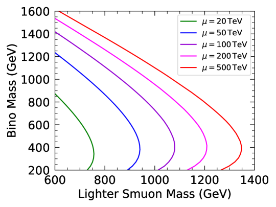
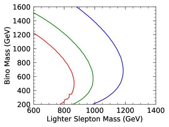
Figure 2: Contours of constant $\mu$ to realize $a_{\mu}^{\rm(SUSY)}=\Delta a_{\mu}^{(0\sigma)}$, taking $\tan\beta=50$, and $m_{L2}=m_{R2}$. The green, blue, violet, magenta, and red contours are for $\mu=20$, $50$, $100$, $200$, and $500\ {\rm TeV}$, respectively.

Figure 3: The boundary between the regions with and without the charge-breaking absolute minimum of the potential, taking $a_{\mu}^{\rm(SUSY)}=\Delta a_{\mu}^{(0\sigma)}$ (red), $\Delta a_{\mu}^{(1\sigma)}$ (green), and $\Delta a_{\mu}^{(2\sigma)}$ (blue). Here, we take $\tan\beta=50$, and $m_{L2}=m_{R2}$.

With the $\mu$ parameter being enhanced, there may appear a charge-breaking minimum of the potential at which sfermions (as well as Higgses) acquire non-vanishing expectation values. The energy density of the charge breaking minimum is often smaller than that of the EW vacuum; if so, the EW vacuum is not absolutely stable. In Fig. 3, on the lighter smuon mass vs. Bino mass plane, we show the parameter region in which the charge breaking minimum becomes the true vacuum; the contours in the figure show the boundary between the regions with and without the charge breaking absolute minimum. Here we take $\tan\beta=50$ and $m_{L2}=m_{R2}$; the red, green, and blue contours are for $a_{\mu}^{\rm(SUSY)}=\Delta a_{\mu}^{(0\sigma)}$, $\Delta a_{\mu}^{(1\sigma)}$, and $\Delta a_{\mu}^{(2\sigma)}$, respectively. The EW vacuum becomes unstable at the right-hand side of the contours.

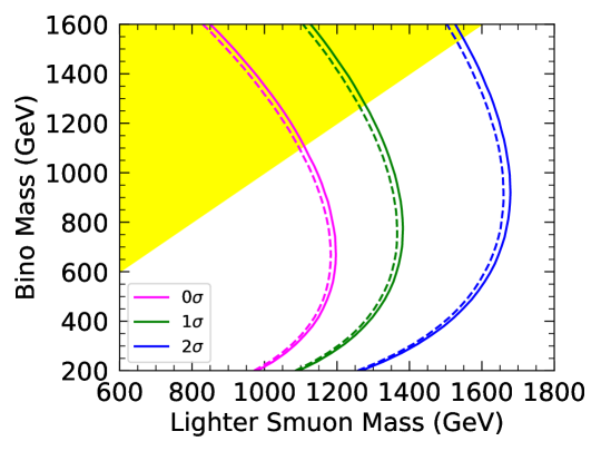
Figure 4: Contours of $S_{\rm eff}=387$, corresponding to $\gamma_{\rm EW}=t_{\rm now}^{-1}$, for the case of $m_{L2}=m_{R2}$. Magenta, green, and blue contours are for $a_{\mu}^{\rm(SUSY)}=\Delta a_{\mu}^{(0\sigma)}$, $\Delta a_{\mu}^{(1\sigma)}$, and $\Delta a_{\mu}^{(2\sigma)}$, respectively, with $\tan\beta=10$ (solid) and $50$ (dashed). In the yellow-shaded region, the lighter smuon becomes lighter than the Bino.

Even if the EW vacuum is unstable, we may still live on it if its lifetime is (much) longer than the present cosmic age. We calculate the decay rate of the EW vacuum using the formulas given in the previous section. Then, we derive constraints on the parameter space.

In Fig. 4, we show the contours of $S_{\rm eff}=387$ on the lighter smuon mass vs. Bino mass plane, taking $a_{\mu}^{\rm(SUSY)}=\Delta a_{\mu}^{(0\sigma)}$, $\Delta a_{\mu}^{(1\sigma)}$, and $\Delta a_{\mu}^{(2\sigma)}$. Here, we take $m_{L2}=m_{R2}$ and $\tan\beta=10$ and $50$. The value of $S_{\rm eff}$ becomes smaller as the smuons become heavier; thus the contours in the figures show the maximal possible value of the lighter smuon mass for a given Bino mass. Notice that, as discussed in Ref. [Chigusa:2022xpq], the upper bound on the lighter smuon mass becomes smaller as the ratio $m_{L2}/m_{R2}$ deviates from $1$; thus the bound is obtained from the study of the case of $m_{L2}=m_{R2}$. In the figure, we show the region in which the lighter smuon becomes lighter than the Bino. In such a parameter region, the lighter smuon becomes the lightest among the MSSM particles and it may be the lightest superparticle (LSP). The LSP is stable assuming $R$-parity conservation. If the lighter smuon is the LSP and is stable, collider and cosmological constraints may apply. The LHC experiment excludes stable sleptons lighter than $\sim 430\ {\rm GeV}$ [CMS:2016kce, ATLAS:2019gqq]. In addition, cosmologically, the existence of a new stable charged particle is disfavored because it can be produced just after the hot big bang and survives until today. These constraints are, however, evaded if there exists a superparticle lighter than the smuon; the examples include gravitino (i.e., the superpartner of the graviton) and axino (i.e., superpartner of the axion). An $R$-parity violation is another possibility to avoid the constraints. Because these constraints are model dependent, we do not take them into account in deriving the vacuum stability bound on the smuon mass.

The vacuum stability bound becomes severer as the value of $a_{\mu}^{\rm(SUSY)}$ becomes larger. In Fig. 5, we show the maximal possible value of the lighter smuon mass as a function of $a_{\mu}^{\rm(SUSY)}$, taking $m_{L2}=m_{R2}$. For the case of adopting the SM prediction given in Eq. (2.2), with which the SM prediction deviates from the experimental value by $4.2\sigma$, the constraint is stringent; requiring $0\sigma$, $1\sigma$, and $2\sigma$ consistency, the lighter smuon mass is required to be smaller than $1.18$, $1.37$, and $1.66\ {\rm TeV}$, respectively, for $\tan\beta=50$. On the contrary, if we adopt the lattice evaluation of the HVP contribution, the bound on the smuon mass becomes less stringent. For example, even if we require that the SM prediction be equal to the central value of $a_{\mu}^{\rm(exp)}$, the lighter smuon mass can be as heavy as $1.86\ {\rm TeV}$ taking $a_{\mu}^{\rm(SM,BMW)}$ as SM prediction.

Figure 5: Maximal possible value of the lighter smuon mass as a function of $a_{\mu}^{\rm(SUSY)}$, taking $m_{L2}=m_{R2}$. Solid and dashed lines are for $\tan\beta=10$ and $50$, respectively.

5.2 Case with three generations of sleptons

Next, we consider the case that all the slepton masses are comparable. In such a case, the stau sector has the most serious effect on the stability of the EW vacuum.

The value of $\mu$ necessary to solve the muon $g-2$ anomaly is (almost) unchanged even with relatively light staus. With the value of $\mu$ suggested from the muon $g-2$ anomaly, the trilinear coupling of staus may be significantly enhanced; it is an order of magnitude larger than that of smuons because the trilinear couplings of sfermions are proportional to corresponding Yukawa coupling constants (as far as we can neglect the so-called $A$-terms, i.e., soft SUSY breaking trilinear couplings). Consequently, if the smuon and stau masses are comparable, the EW vacuum is more easily destabilized by the trilinear coupling of the staus.

We study the decay of the EW vacuum mediated by the bounce configuration consisting of staus and Higgses. For simplicity, we assume that superparticles other than the sleptons and the Bino are much heavier than the EW scale so that the decay rate of the EW vacuum can be studied by the EFT containing only the sleptons and the Bino (as well as the SM particles).

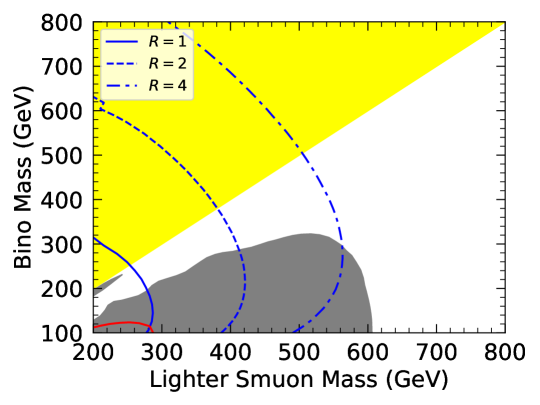
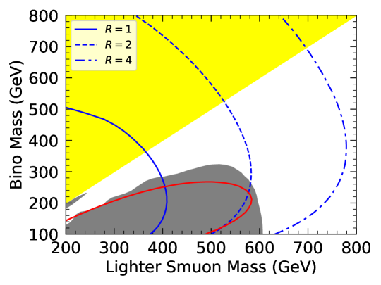
Figure 6: Contours of constant $S_{\rm eff}=387$ for $a_{\mu}^{\rm(SUSY)}=\Delta a_{\mu}^{(0\sigma)}$ with $R=1$ (solid), $2$ (dashed), and $4$ (dash-dotted), taking $\tan\beta=50$. Here, we assume $m_{\tilde{e}_{L}}=m_{\tilde{e}_{R}}=m_{\tilde{\mu}_{L}}=m_{\tilde{\mu}_{R}}$ and $m_{\tilde{\tau}_{L}}=m_{\tilde{\tau}_{R}}$, and parameterize the stau masses as $m_{\tilde{\tau}_{L,R}}=R\,m_{\tilde{\mu}_{L,R}}$. The gray-shaded region is excluded by the ATLAS searches for the smuons assuming that the lightest neutralino is the LSP, while the lighter smuon becomes lighter than the Bino in the yellow-shaded region. In addition, the red contour shows the boundary beyond which the lighter stau becomes the lightest MSSM particle.

Figure 7: Same as Fig. 7, except for the case of $a_{\mu}^{\rm(SUSY)}=\Delta a_{\mu}^{(2\sigma)}$.

In order to see how the upper bound on the lighter smuon mass depends on the mass hierarchy between the smuons and staus, we take $m_{\tilde{e}_{L}}=m_{\tilde{e}_{R}}=m_{\tilde{\mu}_{L}}=m_{\tilde{\mu}_{R}}$ and $m_{\tilde{\tau}_{L}}=m_{\tilde{\tau}_{R}}$, and parameterize the stau masses as follows:

$$m_{\tilde{\tau}_{L,R}}=R\,m_{\tilde{\mu}_{L,R}},$$ (5.3)

where $R$ is a positive constant. In Figs. 7 and 7, we show the contours of constant $S_{\rm eff}=387$ on the lighter smuon mass vs. Bino mass plane, taking $R=1$, $2$ and $4$. We consider the cases of $a_{\mu}^{\rm(SUSY)}=\Delta a_{\mu}^{(0\sigma)}$ and $\Delta a_{\mu}^{(2\sigma)}$ in Figs. 7 and 7, respectively.

If all the slepton masses are of the same order, the lighter stau may become the LSP. This is because the lighter stau mass may be significantly reduced due to the large left-right stau mixing. In the present case, the lighter stau becomes the lightest MSSM particle in a wide parameter space when $R$ becomes close to $1$ (or smaller). In Figs. 7 and 7, we show the contour beyond which the lighter stau becomes the lightest MSSM particle for the case of $R=1$ (red contour). (For the cases of $R=2$ and $4$, we have checked that the stau does not become the LSP in the parameter region of our interest.) In addition, as in the case of Fig. 4, we show the region in which the lighter smuon becomes lighter than the Bino (yellow-shaded region). We also show the region which is excluded by the smuon searches by the ATLAS experiment (gray region) [ATLAS:2022rcw]. For $R=1$, the stau can be the LSP in a wide parameter region; such a parameter region may conflict with the LHC constraint on the stable slepton because the stable slepton lighter than $\sim 430\ {\rm GeV}$ is excluded by the LHC [CMS:2016kce, ATLAS:2019gqq]. In addition, cosmological constraints on stable charged particles may also apply. However, as we have mentioned, these constraints are model dependent and hence we do not take them into account to derive a conservative bound.

To see how the upper bound depends on the ratio of the stau and smuon masses, in Fig. 8, we show the maximal possible value of the lighter smuon mass to guarantee the longevity of the EW vacuum as a function of $R$; here we take $a_{\mu}^{\rm(SUSY)}=\Delta a_{\mu}^{(0\sigma)}$ (magenta), $\Delta a_{\mu}^{(1\sigma)}$ (green), and $\Delta a_{\mu}^{(2\sigma)}$ (blue). We can see that the upper bound on the lighter smuon mass is significantly lowered compared with the case only with the smuons.

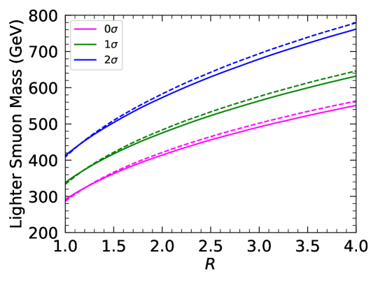
Figure 8: Upper bound on the lighter smuon mass as a function of $R$. The magenta, green, and blue lines show the bound for $a_{\mu}^{\rm(SUSY)}=\Delta a_{\mu}^{(0\sigma)}$, $\Delta a_{\mu}^{(1\sigma)}$, and $\Delta a_{\mu}^{(2\sigma)}$, respectively, taking $\tan\beta=10$ (solid) and $50$ (dashed). Here, we assume $m_{\tilde{e}_{L}}=m_{\tilde{e}_{R}}=m_{\tilde{\mu}_{L}}=m_{\tilde{\mu}_{R}}$ and $m_{\tilde{\tau}_{L}}=m_{\tilde{\tau}_{R}}$, and parameterize the stau masses as $m_{\tilde{\tau}_{L,R}}=R\,m_{\tilde{\mu}_{L,R}}$.

6 Conclusions and Discussion

In this paper, we have studied the stability of the EW vacuum in the MSSM, paying particular attention to its relation to the SUSY contribution to the muon anomalous magnetic moment, $a_{\mu}$. The recent measurement of $a_{\mu}$ suggests a significant deviation from the SM prediction if the HVP contribution is evaluated based on the $R$-ratio. One possible solution to such a deviation is to introduce a sizable SUSY contribution to $a_{\mu}$. However, such a possibility may conflict with the stability of the EW vacuum because a large trilinear scalar coupling, which is necessary to enhance the SUSY contribution to $a_{\mu}$, may destabilize the EW vacuum.

We have performed a detailed analysis of the stability of the EW vacuum in the MSSM. We first give a complete formula to perform a full one-loop calculation of the decay rate. The one-loop calculation is necessary to determine the overall factor of the decay rate as well as to reduce its renormalization-scale dependence. The one-loop contribution to the decay rate can be evaluated by solving relevant differential equations; we have given a set of differential equations for the calculation of the decay rate in the MSSM. The counter terms to remove the ultra-violet divergences are also given in the $\overline{\rm MS}$-scheme.

Then, we have calculated the decay rate of the EW vacuum and derived an upper bound on the lighter smuon mass. In our procedure, we have numerically calculated the bounce configuration with using the gradient-flow method. Once we obtain the bounce, we derive the fluctuation operators, which give the differential equations to be solved for the calculation of the one-loop contribution. We have numerically solved the differential equations and calculated the one-loop effects on the decay rate with properly removing the divergences adopting the $\overline{\rm MS}$ scheme. The upper bound on the lighter smuon mass has been obtained as a function of the SUSY contribution to the muon anomalous magnetic moment. Requiring $1\sigma$ ($2\sigma$) consistency between the experimentally measured and theoretically predicted values of $a_{\mu}$ adopting the HVP contribution based on the $R$-ratio, the smuon mass is required to be lighter than $1.37\ {\rm TeV}$ ($1.66\ {\rm TeV}$). Notice, however, that the upper bound can be relaxed if we adopt the HVP contribution based on the recent lattice results.

Acknowledgments: S.C. is supported by the Director, Office of Science, Office of High Energy Physics of the U.S. Department of Energy under the Contract No. DE-AC02-05CH1123. T.M. is supported by JSPS KAKENHI Grant Number 22H01215. Y.S. is supported by I-CORE Program of the Israel Planning Budgeting Committee (grant No. 1937/12).

Appendix A Beta Functions

In this appendix, we summarize the one-loop beta functions of the slepton EFT used in our analysis, whose Lagrangian is given by Eq. (3.9). Hereafter, we use a matrix notation of the EFT couplings expressed by simply suppressing the flavor indices. Note that some of the couplings, i.e., $\lambda_{HR}$, $\lambda_{HL}$, ${\kappa^{\prime}}$, $m_{R}^{2}$, and $m_{L}^{2}$, have only one flavor index and form diagonal matrices, while some of the couplings, i.e., the Yukawa couplings, $T$, $m_{L}^{2}$, and $m_{R}^{2}$, are diagonal simply because we neglect the flavor-violating effect. (See the discussion at the end of this section for the consistency of our treatment.) We define the beta function of a coupling constant $X$ with

$$\beta_{X}\equiv\frac{d}{dt}X,$$ (A.1)

where $t\equiv\ln Q$ with $Q$ being the renormalization scale.

Taking the $SU(5)$ normalization of the $U(1)_{Y}$ coupling, one-loop beta functions of the gauge couplings are given by

$$\beta_{g_{a}}=\frac{b_{a}}{16\pi^{2}}g_{a}^{3}~{}~{}(a=1,2,3),$$ (A.2)

with

$$(b_{1},b_{2},b_{3})=\left(\frac{41}{10}+\frac{3}{20}N_{f},-\frac{19}{6}+\frac{1}{12}N_{f},-7\right),$$ (A.3)

where the number of slepton flavors is $N_{f}=1$ $(3)$ when only smuon is considered (three generations of sleptons are considered).

One-loop beta functions of the Yukawa couplings are given by

$$(16\pi^{2})\beta_{Y_{\ell}}= \left(Y_{2}(H)+\frac{3}{2}Y_{\ell}^{2}+\frac{1}{2}Y_{R}^{2}+\frac{1}{2}Y_{L}^{2}-\frac{9}{4}g_{2}^{2}-\frac{9}{4}g_{1}^{2}\right)Y_{\ell},$$ (A.4)

$$(16\pi^{2})\beta_{Y_{R}}= \left(\mathrm{Tr}\left[Y_{L}^{2}+\frac{1}{2}Y_{R}^{2}\right]+Y_{\ell}^{2}+\frac{3}{2}Y_{R}^{2}-\frac{9}{5}g_{1}^{2}\right)Y_{R},$$ (A.5)

$$(16\pi^{2})\beta_{Y_{L}}= \left(\mathrm{Tr}\left[Y_{L}^{2}+\frac{1}{2}Y_{R}^{2}\right]+\frac{1}{2}Y_{\ell}^{2}+\frac{3}{2}Y_{L}^{2}-\frac{9}{4}g_{2}^{2}-\frac{9}{20}g_{1}^{2}\right)Y_{L},$$ (A.6)

with

$$Y_{2}(H)\equiv\mathrm{Tr}\left[3Y_{u}^{2}+3Y_{d}^{2}+Y_{\ell}^{2}\right],$$ (A.7)

where $Y_{u}$ and $Y_{d}$ are the SM-like Yukawa couplings of the up-type and down-type quarks, respectively. Note that, since we neglect the flavor- and CP-violating effects, we do not need to carefully treat the ordering of matrix products and Hermite conjugate of Yukawa coupling matrices.

One-loop beta functions of the scalar quartic couplings are given by

$$(16\pi^{2})\beta_{\lambda_{H}}= 24\lambda_{H}^{2}+\left(4Y_{2}(H)-9g_{2}^{2}-\frac{9}{5}g_{1}^{2}\right)\lambda_{H}+\Tr(\lambda_{HL}^{2}+\lambda_{HR}^{2}+{\kappa^{\prime}}^{2})$$

$$-2Y_{4}(H)+\frac{9}{8}g_{2}^{4}+\frac{9}{20}g_{2}^{2}g_{1}^{2}+\frac{27}{200}g_{1}^{4},$$ (A.8)

$$(16\pi^{2})\beta_{\lambda_{R}}= 4(2F-I)\circ\lambda_{R}^{2}+8(F+I)\circ\lambda_{R}\circ\lambda_{R}+2\lambda_{LR}\lambda_{LR}^{T}+2\lambda_{HR}F\lambda_{HR}$$

$$+2Y_{R}^{2}\lambda_{R}+2\lambda_{R}Y_{R}^{2}-\frac{36}{5}g_{1}^{2}\lambda_{R}-2Y_{R}^{2}FY_{R}^{2}+\frac{54}{25}g_{1}^{4}F,$$ (A.9)

$$(16\pi^{2})\beta_{\lambda_{L}}= 4(3F-I)\circ\lambda_{L}^{2}+8(F+I)\circ\lambda_{L}\circ\lambda_{L}+4(\lambda_{L}\lambda^{\prime}_{L}+\lambda^{\prime}_{L}\lambda_{L})$$

$$+4\lambda_{L}^{{}^{\prime}2}+4\lambda^{\prime}_{L}\circ\lambda^{\prime}_{L}+\lambda_{LR}^{T}\lambda_{LR}+\lambda_{HL}^{2}+{\kappa^{\prime}}^{2}+\lambda_{HL}(F-I){\kappa^{\prime}}+{\kappa^{\prime}}(F-I)\lambda_{HL}$$

$$+2Y_{L}^{2}\lambda_{L}+2\lambda_{L}Y_{L}^{2}-\left(9g_{2}^{2}+\frac{9}{5}g_{1}^{2}\right)\lambda_{L}-2Y_{L}^{2}FY_{L}^{2}$$

$$+\left(\frac{9}{8}g_{2}^{4}+\frac{27}{200}g_{1}^{4}\right)F-\frac{9}{20}g_{2}^{2}g_{1}^{2}(F-2I),$$ (A.10)

$$(16\pi^{2})\beta_{\lambda^{\prime}_{L}}= (F-I)\circ\Bigl{(}4(\lambda_{L}\lambda^{\prime}_{L}+\lambda^{\prime}_{L}\lambda_{L})+16\lambda_{L}\circ\lambda^{\prime}_{L}+8\lambda^{\prime}_{L}\circ\lambda^{\prime}_{L}-4Y_{L}^{4}\Bigr{)}$$

$$+(\lambda_{HL}-{\kappa^{\prime}})(F-I)(\lambda_{HL}-{\kappa^{\prime}})$$

$$+2Y_{L}^{2}\lambda^{\prime}_{L}+2\lambda^{\prime}_{L}Y_{L}^{2}-\left(9g_{2}^{2}+\frac{9}{5}g_{1}^{2}\right)\lambda^{\prime}_{L}+\frac{9}{10}g_{2}^{2}g_{1}^{2}(F-I)$$ (A.11)

$$(16\pi^{2})\beta_{\lambda_{LR}}= 4\lambda_{LR}\circ\lambda_{LR}+8\lambda_{LR}\lambda_{L}+4I\circ\lambda_{LR}\circ\lambda_{L}+4((F-I)\circ\lambda_{LR})(I\circ\lambda_{L})$$

$$+4\lambda_{LR}\lambda^{\prime}_{L}+4\lambda_{R}\lambda_{LR}+4I\circ\lambda_{R}\circ\lambda_{LR}+4(I\circ\lambda_{R})((F-I)\circ\lambda_{LR})$$

$$+2\lambda_{HR}F(\lambda_{HL}+{\kappa^{\prime}})$$

$$+2\lambda_{LR}Y_{L}^{2}+2Y_{R}^{2}\lambda_{LR}-\left(\frac{9}{2}g_{2}^{2}+\frac{9}{2}g_{1}^{2}\right)\lambda_{LR}$$

$$-4Y_{R}^{2}FY_{L}^{2}+\frac{27}{25}g_{1}^{4}F,$$ (A.12)

$$(16\pi^{2})\beta_{\lambda_{HR}}= 4\lambda_{HR}^{2}+2f(\lambda_{LR},\lambda_{HL}+{\kappa^{\prime}})$$

$$+f\left(12\lambda_{H}+4\lambda_{R}+4I\circ\lambda_{R}+2Y_{2}(H)+2Y_{R}^{2}-\frac{9}{2}g_{2}^{2}-\frac{9}{2}g_{1}^{2},\lambda_{HR}\right)$$

$$-4Y_{\ell}^{2}Y_{R}^{2}+\frac{27}{25}g_{1}^{4},$$ (A.13)

$$(16\pi^{2})\beta_{\lambda_{HL}}= 6\lambda_{HL}^{2}-4\lambda_{HL}{\kappa^{\prime}}+2{\kappa^{\prime}}^{2}+4f(\lambda_{H}+\lambda_{L},{\kappa^{\prime}})+2f(\lambda_{LR}^{T},\lambda_{HR})$$

$$+f\left(8\lambda_{H}+4\lambda_{L}+4I\circ\lambda_{L}+4\lambda^{\prime}_{L}+2Y_{2}(H)+2Y_{L}^{2}-9g_{2}^{2}-\frac{9}{5}g_{1}^{2},\lambda_{HL}\right)$$

$$+\frac{9}{4}g_{2}^{4}+\frac{9}{10}g_{2}^{2}g_{1}^{2}+\frac{27}{100}g_{1}^{4},$$ (A.14)

$$(16\pi^{2})\beta_{{\kappa^{\prime}}}= 6{\kappa^{\prime}}^{2}-4\lambda_{HL}{\kappa^{\prime}}+2\lambda_{HL}^{2}+4f(\lambda_{H}+\lambda_{L},\lambda_{HL})+2f(\lambda_{LR}^{T},\lambda_{HR})$$

$$+f\left(8\lambda_{H}+4\lambda_{L}+4I\circ\lambda_{L}+4\lambda^{\prime}_{L}+2Y_{2}(H)+2Y_{L}^{2}-9g_{2}^{2}-\frac{9}{5}g_{1}^{2},{\kappa^{\prime}}\right)$$

$$-4Y_{\ell}^{2}Y_{L}^{2}+\frac{9}{4}g_{2}^{4}-\frac{9}{10}g_{2}^{2}g_{1}^{2}+\frac{27}{100}g_{1}^{4},$$ (A.15)

where

$$Y_{4}(H) \equiv\mathrm{Tr}\left[3Y_{u}^{4}+3Y_{d}^{4}+Y_{\ell}^{4}\right],$$ (A.16)

and $I$ and $F$ are constant matrices defined as

$$I\equiv\begin{pmatrix}1&0&0\\ 0&1&0\\ 0&0&1\end{pmatrix},~{}~{}~{}F\equiv\begin{pmatrix}1&1&1\\ 1&1&1\\ 1&1&1\end{pmatrix}.$$ (A.17)

We also use the Hadamard product defined through

$$(M\circ N)_{\alpha\beta} \equiv M_{\alpha\beta}N_{\alpha\beta},$$ (A.18)

and a matrix operation that maps a diagonal matrix $D$ to another diagonal matrix

$$f(M,D)=I\circ(MDF).$$ (A.19)

Finally, one-loop beta functions of dimensionful parameters are given by

$$(16\pi^{2})\beta_{T}= \left(Y_{2}(H)-\frac{9}{2}g_{2}^{2}-\frac{27}{10}g_{1}^{2}\right)T+TY_{L}^{2}+Y_{R}^{2}T$$

$$+2\lambda_{HR}T+T\left(-2\lambda_{HL}+4{\kappa^{\prime}}\right)+2\lambda_{LR}\circ T-4M_{1}Y_{\ell}Y_{R}Y_{L},$$ (A.20)

$$(16\pi^{2})\beta_{M_{1}}= \mathrm{Tr}\left(2Y_{L}^{2}+Y_{R}^{2}\right)M_{1},$$ (A.21)

$$(16\pi^{2})\beta_{m_{H}^{2}}= \left(12\lambda_{H}+2Y_{2}(H)-\frac{9}{2}g_{2}^{2}-\frac{9}{10}g_{1}^{2}\right)m_{H}^{2}$$

$$+\mathrm{Tr}\left[2(\lambda_{HL}+{\kappa^{\prime}})m_{L}^{2}+2\lambda_{HR}m_{R}^{2}+2T^{2}\right],$$ (A.22)

$$(16\pi^{2})\beta_{m_{R}^{2}}= f\left(4\lambda_{R}+4I\circ\lambda_{R}-\frac{18}{5}g_{1}^{2},m_{R}^{2}\right)$$

$$+4f(\lambda_{LR},m_{L}^{2})+4m_{H}^{2}\lambda_{HR}+2Y_{R}^{2}m_{R}^{2}-4Y_{R}^{2}M_{1}^{2}+4T^{2},$$ (A.23)

$$(16\pi^{2})\beta_{m_{L}^{2}}= f\left(8\lambda_{L}+4I\circ\lambda_{L}+4\lambda^{\prime}_{L}-\frac{9}{2}g_{2}^{2}-\frac{9}{10}g_{1}^{2},m_{L}^{2}\right)$$

$$+2f(\lambda_{LR}^{T},m_{R}^{2})+2m_{H}^{2}(\lambda_{HL}+{\kappa^{\prime}})+2Y_{L}^{2}m_{L}^{2}-4Y_{L}^{2}M_{1}^{2}+2T^{2}.$$ (A.24)

Note that, with the above beta-functions, the RG flow does not induce off-diagonal elements of the Yukawa couplings, $T$, $m_{R}^{2}$, and $m_{L}^{2}$, as far as we start from boundary conditions with vanishing off-diagonal elements. This ensures the consistency of our treatment.

Appendix B Bounce

In this appendix, we explain how we calculate the bounce configuration. In our analysis, the bounce configuration is numerically calculated by using the gradient flow method [Chigusa:2019wxb, Sato:2019axv]; in particular, we use the modified version proposed in [Sato:2019axv].

Among the various methods to obtain the bounce, the gradient flow method has an advantage in the calculation of fluctuation operators. In the case of our interest, we need to evaluate the functional determinants of the fluctuation operators of the size as large as $7\times 7$. In order to numerically solve the corresponding seven simultaneous differential equations up to a large enough $r$ (see Eqs. (4.13) and (4.14)), the bounce configuration at a large value of $r$ should be well understood. In particular, we need to numerically follow the evolution of the functions $\psi_{\ell}(r)$ and $\hat{\psi}_{\ell}(r)$, whose evolution equations are given by Eqs. (4.13) and (4.14), respectively, until they show the same asymptotic behavior. For the case of multi-field bounce, a precise calculation at $r\rightarrow\infty$ is highly non-trivial because, at $r\rightarrow\infty$, the functions exponentially grow with different growth rates. The gradient flow method ensures that the solutions approach the false vacuum at $r\rightarrow\infty$ with the correct asymptotic behaviors; we found that it stabilizes the calculation of the functional determinant.

Here, the scalar fields responsible for the bounce configuration are denoted as $\rho_{i}$, with $i$ being the index distinguishing the field species. The field values at the true vacuum and the false vacuum are denoted by $v^{\rm(T)}_{i}$ and $v^{\rm(F)}_{i}$, respectively.

We define

$$\mathcal{V} =2\pi^{2}\int_{0}^{\infty}\differential{r}r^{3}V(\rho(r)),$$ (B.1)

$$\mathcal{T} =2\pi^{2}\int_{0}^{\infty}\differential{r}r^{3}\sum_{i}\frac{1}{2}\rho^{\prime 2}_{i}(r),$$ (B.2)

where $V(\rho)$ is the scalar potential with $V(v^{\rm(F)})=0$. It has been shown that a minimization sequence of $\mathcal{T}$ with a fixed $\mathcal{V}$ converges to a non-trivial configuration, which is related to the bounce through the scale transformation [Coleman:1977th]. Such a minimization sequence can be realized by the gradient flow method [Sato:2019axv]. The flow equation is given by

$$\partial_{s}\rho_{i}=\partial_{r}^{2}\rho_{i}+\frac{3}{r}\partial_{r}\rho_{i}-\lambda(\rho)\partialderivative{V}{\rho_{i}},$$ (B.3)

where $s$ is the flow time and

$$\lambda(\rho)=\frac{\sum_{i}\int_{0}^{\infty}\differential{r}r^{3}\partialderivative{V}{\rho_{i}}\quantity[\partial_{r}^{2}\rho_{i}+\frac{3}{r}\partial_{r}\rho_{i}]}{\sum_{i}\int_{0}^{\infty}\differential{r}r^{3}\quantity(\partialderivative{V}{\rho_{i}})^{2}}.$$ (B.4)

Here, $\rho_{i}$ is promoted to a function of $r$ and the flow time $s$.

In our calculation, we use a different radius variable, which is defined as

$$x=\tanh\frac{r}{r_{0}},$$ (B.5)

where $r_{0}$ is a constant. This allows us to set the boundary conditions explicitly,

$$\partial_{x}\rho_{i}(x=0)=0,~{}~{}~{}\rho_{i}(x=1)=v^{\rm(F)}_{i}.$$ (B.6)

In terms of $x$, $\mathcal{V}$ is written as

$$\mathcal{V}=2\pi^{2}r_{0}^{4}\int_{0}^{1}\differential{x}\frac{\operatorname{arctanh}^{3}x}{1-x^{2}}V(\rho),$$ (B.7)

and the flow equation becomes

$$\partial_{s}\rho_{i}=\quantity(1-x^{2})^{2}\partial_{x}^{2}\rho_{i}+(1-x^{2})\quantity(\frac{3}{\operatorname{arctanh}x}-2x)\partial_{x}\rho_{i}-\lambda(\rho)\partialderivative{V}{\rho_{i}},$$ (B.8)

where

$$\lambda(\rho)=\frac{\sum_{i}\int_{0}^{1}\differential{x}\partialderivative{V}{\rho_{i}}\quantity[\quantity(1-x^{2})\partial_{x}^{2}\rho_{i}+\quantity(\frac{3}{\operatorname{arctanh}x}-2x)\partial_{x}\rho_{i}]\operatorname{arctanh}^{3}x}{\sum_{i}\int_{0}^{1}\differential{x}\frac{\operatorname{arctanh}^{3}x}{1-x^{2}}\quantity(\partialderivative{V}{\rho_{i}})^{2}}.$$ (B.9)

We first find an initial field configuration that gives a negative value of $\mathcal{V}$. We take the following configuration:

$$\rho_{i}(x)=\tilde{v}_{i}+\frac{1}{2}[\tanh\{c_{2}(\operatorname{arctanh}x^{2}-c_{3})\}+1](v^{\rm(F)}_{i}-\tilde{v}_{i}),$$ (B.10)

with

$$\tilde{v}_{i}=c_{1}(v^{\rm(T)}_{i}-v^{\rm(F)}_{i})+v^{\rm(F)}_{i},$$ (B.11)

where $c_{i}$’s are constants. In our numerical calculation, we take $c_{3}=0.3$. Then, we start with $(c_{1},c_{2})=(0.001,3)$ and increase them until $\mathcal{V}<0$ is realized.

We numerically solve the flow equation until the right-hand side of Eq. (B.8) becomes small enough. The bounce solution is then obtained as

$$\rho_{i}(r)=\rho_{i}\quantity(\tanh\frac{r}{\sqrt{\lambda}}).$$ (B.12)

Here, $r$ is rescaled so that the solution satisfies the Derrick’s relation, $\mathcal{T}=-2\mathcal{V}$. Notice that all the above formulas are independent of $r_{0}$ and thus we do not need to know the typical size of the bounce before the calculation.

With the bounce configuration given above, the Euclidean action is given by

$$S_{E} =2\pi^{2}\lambda^{2}\int_{0}^{1}\differential{x}\frac{\operatorname{arctanh}^{3}x}{1-x^{2}}\quantity[\frac{(1-x^{2})^{2}}{2\lambda}(\partial_{x}\rho)^{2}+V(\rho(x))].$$ (B.13)

Appendix C Fluctuation Operators

In this appendix, we summarize the fluctuation operators that we use in our calculation. We decompose all the scalar fields into canonically normalized real scalar fields, denoted as $\Phi_{i}$ (with $i$ being the index distinguishing the species of the scalars). The scalars are expanded around the bounce, $\rho_{i}(r)$, as

$$\Phi_{i}=\rho_{i}+\varphi_{i},$$ (C.1)

where $\varphi_{i}$ is the fluctuation around the bounce.

The fluctuation operators for sleptons with $\rho_{i}\neq 0$ are different from those with $\rho_{i}=0$. In the following, we use index $\rho$ for the sleptons with $\rho_{i}\neq 0$ and $I$ for those with $\rho_{i}=0$. More explicitly, when we consider the instability towards the smuon direction assuming the other sfermions are heavy, $\rho=2$ and there is no contribution from other sfermions (i.e., the index $I$ is irrelevant). When we consider the instability towards the stau direction including the other sleptons, $\rho=3$ and $I=1,2$.

The fluctuation operators, $\mathcal{M}^{(A_{\mu}\varphi)}$, $\mathcal{M}^{(c\bar{c})}$ and $\mathcal{M}^{(\psi)}$, are large matrices containing all the fields in EFT, where $\mathcal{M}^{(A_{\mu}\varphi)}$, $\mathcal{M}^{(c\bar{c})}$ and $\mathcal{M}^{(\psi)}$ are those of the gauge bosons and the scalars, the ghosts, and fermions, respectively. However, in practice, they can be block-diagonalized and we can calculate them one by one. We give each block below.

C.1 Scalars that do not mix with gauge bosons

Concerning $\mathcal{M}^{(A_{\mu}\varphi)}$, we find blocks that contain only scalar fluctuations. (Such scalars are denoted by $\phi_{i}$.) Although the fluctuation operators for them can be derived from the formulas with gauge bosons given in the next subsection, we discuss them separately since they have a much simpler structure.

The bounce-dependent mass terms in each block can be denoted as

$$\mathcal{L}_{\phi}=-\frac{1}{2}\Omega_{ij}^{(\phi)}(\rho)\phi_{i}\phi_{j}.$$ (C.2)

Then, the fluctuation operator is given by

$$\mathcal{M}^{(\phi)}=-\partial^{2}+\Omega^{(\phi)}.$$ (C.3)

We expand the scalar fields by using mode functions as

$$\phi=\alpha_{\ell m_{1}m_{2}}^{\phi}(r)Y_{\ell m_{1}m_{2}},$$ (C.4)

where the sum over $\ell,m_{1}$ and $m_{2}$ are implicit. Here, $Y_{\ell m_{1}m_{2}}$ is the hyperspherical harmonics where $\ell$, which is an integer, is the 4D angular momentum quantum number and $m_{1}$ and $m_{2}$ are the quantum numbers that correspond to the magnetic quantum number. Then,

$$\partial^{2}\alpha_{\ell m_{1}m_{2}}^{\phi}Y_{\ell m_{1}m_{2}}=\quantity(\Delta_{\ell}\alpha_{\ell m_{1}m_{2}}^{\phi})Y_{\ell m_{1}m_{2}},$$ (C.5)

where

$$\Delta_{\ell}\equiv\partial_{r}^{2}+\frac{3}{r}\partial_{r}-\frac{\ell(\ell+2)}{r^{2}}.$$ (C.6)

Since the bounce is $O(4)$-symmetric, there is no mixing among different angular momenta and the contribution to the prefactor is given by

$$\mathcal{A}^{(\phi)}=-\frac{1}{2}\ln\frac{\det\mathcal{M}^{(\phi)}}{\det\widehat{\mathcal{M}}^{(\phi)}}=-\frac{1}{2}\sum_{\ell=0}^{\infty}(\ell+1)^{2}\ln\frac{\det\mathcal{M}_{\ell}^{(\phi)}}{\det\widehat{\mathcal{M}}_{\ell}^{(\phi)}},$$ (C.7)

where

$$\mathcal{M}_{\ell}^{(\phi)}=-\Delta_{\ell}+\Omega^{(\phi)}.$$ (C.8)

Notice that $(\ell+1)^{2}$ is the degeneracy factor due to $m_{1}$ and $m_{2}$.

C.1.1 Scalars with $\rho^{\prime}_{i}(r)\neq 0$

We first consider fluctuations of the fields which the bounce consists of, i.e., $\real H^{0}$, $\real\tilde{\ell}_{L\rho}^{-}$, and $\real\tilde{\ell}_{R\rho}$. Because of the $U(1)_{\rm EM}$ breaking due to the bounce, neutral and charged components mix with each other. They include the fluctuations corresponding to the translation of the bounce, and hence there appear translational zero modes for $\ell=1$.

In the basis of $(\real H^{0},\real\tilde{\ell}_{L\rho}^{-},\real\tilde{\ell}_{R\rho})/\sqrt{2}$, the bounce-dependent mass matrix is given by

$$\Omega_{11}^{(\rho)} =m_{H}^{2}+\frac{\lambda_{HR\rho}}{2}\rho_{R}^{2}+3\lambda_{H}\rho_{h}^{2}+\frac{\kappa^{\prime}_{\rho}}{2}\rho_{L}^{2},$$ (C.9)

$$\Omega_{12}^{(\rho)} =-\frac{T_{\rho}}{\sqrt{2}}\rho_{e}+\kappa^{\prime}_{\rho}\rho_{h}\rho_{L},$$ (C.10)

$$\Omega_{13}^{(\rho)} =-\frac{T_{\rho}}{\sqrt{2}}\rho_{L}+\lambda_{HR\rho}\rho_{R}\rho_{h},$$ (C.11)

$$\Omega_{22}^{(\rho)} =m_{L\rho}^{2}+\frac{\lambda_{LR\rho\rho}}{2}\rho_{R}^{2}+\frac{\kappa^{\prime}_{\rho}}{2}\rho_{h}^{2}+3\lambda_{L\rho\rho}\rho_{L}^{2},$$ (C.12)

$$\Omega_{23}^{(\rho)} =-\frac{T_{\rho}}{\sqrt{2}}\rho_{h}+\lambda_{LR\rho\rho}\rho_{R}\rho_{L},$$ (C.13)

$$\Omega_{33}^{(\rho)} =m_{R\rho}^{2}+3\lambda_{R\rho\rho}\rho_{R}^{2}+\frac{\lambda_{HR\rho}}{2}\rho_{h}^{2}+\frac{\lambda_{LR\rho\rho}}{2}\rho_{L}^{2}.$$ (C.14)

C.1.2 Sleptons with $\rho_{i}(r)=0$

In the case of three generations of sleptons, $\tilde{\ell}_{LI}$ and $\tilde{\ell}_{RI}$ do not mix with gauge bosons. Fluctuation operators of these fields can be decomposed into those for the neutral and charged fields.

The neutral fields, $\real\tilde{\ell}_{LI}^{0}/\sqrt{2}$ and $\imaginary\tilde{\ell}_{LI}^{0}/\sqrt{2}$, have the bounce-dependent mass of

$$\Omega^{(N)}=m_{LI}^{2}+\frac{\lambda_{LR\rho I}}{2}\rho_{R}^{2}+\frac{\lambda_{HLI}}{2}\rho_{h}^{2}+\lambda_{L\rho I}\rho_{L}^{2}.$$ (C.15)

The fluctuation operators of the charged fields become $2\times 2$; those of $(\real\tilde{\ell}_{LI}^{-},\real\tilde{\ell}_{RI})/\sqrt{2}$ and $(-\imaginary\tilde{\ell}_{LI}^{-},\imaginary\tilde{\ell}_{RI})/\sqrt{2}$ are both derived by using the following bounce-dependent mass matrix:

$$\Omega^{(C)}=\matrixquantity(m_{LI}^{2}+\frac{\lambda_{LR\rho I}}{2}\rho_{R}^{2}+\frac{\kappa^{\prime}_{I}}{2}\rho_{h}^{2}+(\lambda_{L\rho I}+\lambda^{\prime}_{L\rho I})\rho_{L}^{2}&-\frac{T_{I}}{\sqrt{2}}\rho_{h}\\ -\frac{T_{I}}{\sqrt{2}}\rho_{h}&m_{RI}^{2}+\lambda_{R\rho I}\rho_{R}^{2}+\frac{\lambda_{HRI}}{2}\rho_{h}^{2}+\frac{\lambda_{LRI\rho}}{2}\rho_{L}^{2}).$$ (C.16)

C.2 Gauge bosons and scalars that mix with each other

Here, we give the fluctuation operators for the blocks that have both the gauge boson fluctuations and the scalar fluctuations. We work in the background gauge with the gauge fixing parameter being $\xi=1$. The gauge fixing terms are given by

$$\mathcal{L}_{\rm GF}=\frac{1}{2}\sum_{a}(\partial^{\mu}A_{\mu}^{a}-\varphi^{i}M_{ia})^{2},$$ (C.17)

where

$$M_{ia}=-g_{a}\tau^{a}_{ij}\rho_{j},$$ (C.18)

and $\tau^{a}_{ij}$ is the generators of the gauge group acting on real fields:

$$D_{\mu}\Phi_{i}\equiv\partial_{\mu}\Phi_{i}+\sum_{a}g_{a}A^{a}_{\mu}\tau^{a}_{ij}\Phi_{j}.$$ (C.19)

Here, $g_{a}$’s are the gauge couplings and $A^{a}_{\mu}$’s are the gauge bosons, namely the photon, the $Z$ boson and the $W$ bosons. The index $a$ runs over all the gauge bosons and $i$ runs over all the scalars. Since we do not break the $SU(3)_{C}$ symmetry, the gluons do not contribute to the decay rate at the one-loop level. In addition, the bounce-dependent mass terms of the Nambu-Goldstone bosons (and the scalars that mix with them) are given in the following form:

$$\mathcal{L}=-\frac{1}{2}\Omega_{ij}^{\rm(NG)}(\rho)\varphi_{i}\varphi_{j}.$$ (C.20)

Then, the fluctuation operator of scalar and gauge bosons are given by

$$\mathcal{M}^{(A_{\mu}\varphi)}=\matrixquantity((-\partial^{2}+M^{t}M)\delta_{\mu\nu}&2(\partial_{\nu}M)^{t}\\ 2(\partial_{\nu}M)&-\partial^{2}+\Omega^{\rm(NG)}+MM^{t}).$$ (C.21)

There also exist contributions from the Faddeev-Popov ghosts. The fluctuation operator of the ghosts is given by

$$\mathcal{M}^{(c\bar{c})}=-\partial^{2}+M^{t}M,$$ (C.22)

which has the degeneracy of two.

We expand the scalar fields and the Faddeev-Popov ghosts with the hyperspherical functions, while the gauge bosons are expanded as

$$A^{a}_{\mu}= \,\alpha^{a}_{S\ell m_{1}m_{2}}(r)\frac{x_{\mu}}{r}Y_{\ell m_{1}m_{2}}+\alpha^{a}_{L\ell m_{1}m_{2}}(r)\frac{r}{L}\partial_{\mu}Y_{\ell m_{1}m_{2}}$$

$$+\alpha^{a}_{T1\ell m_{1}m_{2}}(r)i\epsilon_{\mu\nu\rho\sigma}V_{\nu}^{(1)}L_{\rho\sigma}Y_{\ell m_{1}m_{2}}+\alpha^{a}_{T2\ell m_{1}m_{2}}(r)i\epsilon_{\mu\nu\rho\sigma}V_{\nu}^{(2)}L_{\rho\sigma}Y_{\ell m_{1}m_{2}},$$ (C.23)

where $V_{\nu}^{(i)}$’s are arbitrary independent vectors and

$$L_{\mu\nu}=\frac{i}{\sqrt{2}}(x_{\mu}\partial_{\nu}-x_{\nu}\partial_{\mu}).$$ (C.24)

The $\ell>0$ contributions from the ghost and the contributions from $\alpha^{a}_{T1\ell m_{1}m_{2}}$ and $\alpha^{a}_{T2\ell m_{1}m_{2}}$ are canceled out and we are left with

$$\mathcal{A}^{(A_{\mu}\varphi c\bar{c})} =\ln\frac{\det\mathcal{M}^{(c\bar{c})}}{\det\widehat{\mathcal{M}}^{(c\bar{c})}}-\frac{1}{2}\ln\frac{\det\mathcal{M}^{(A_{\mu}\varphi)}}{\det\widehat{\mathcal{M}}^{(A_{\mu}\varphi)}}$$

$$=\ln\frac{\det\mathcal{M}_{0}^{(c\bar{c})}}{\det\widehat{\mathcal{M}}_{0}^{(c\bar{c})}}-\frac{1}{2}\ln\frac{\det\mathcal{M}_{0}^{(S\varphi)}}{\det\widehat{\mathcal{M}}_{0}^{(S\varphi)}}-\frac{1}{2}\sum_{\ell=1}^{\infty}(\ell+1)^{2}\ln\frac{\det\mathcal{M}_{\ell}^{(SL\varphi)}}{\det\widehat{\mathcal{M}}_{\ell}^{(SL\varphi)}},$$ (C.25)

where

(C.26)

We block-diagonalize the above operators; each block is given below.

C.2.1 Charged gauge bosons

Here, we give the fluctuation operators for $W^{1}$, $W^{2}$, and the scalars that mix with them. For $W^{1}$, the basis of the scalars is $(\imaginary H^{+},\imaginary\ell_{L\rho}^{0})/\sqrt{2}$. For $W^{2}$, it is $(\real H^{+},\real\tilde{\ell}_{L\rho}^{0})/\sqrt{2}$. The fluctuation operator is constructed by

$$M^{(W\pm)}=\matrixquantity(\frac{g_{2}}{2}\rho_{h}\\ \frac{g_{2}}{2}\rho_{L}),$$ (C.27)

and

$$\Omega^{(W\pm)}=\matrixquantity(m_{H}^{2}+\frac{\lambda_{HR\rho}}{2}\rho_{R}^{2}+\lambda_{H}\rho_{h}^{2}+\frac{\lambda_{HL\rho}}{2}\rho_{L}^{2}&-\frac{T_{\rho}}{\sqrt{2}}\rho_{R}+\frac{\kappa_{\rho}}{2}\rho_{h}\rho_{L}\\ -\frac{T_{\rho}}{\sqrt{2}}\rho_{R}+\frac{\kappa_{\rho}}{2}\rho_{h}\rho_{L}&m_{L\rho}^{2}+\frac{\lambda_{HL\rho}}{2}\rho_{h}^{2}+\frac{\lambda_{LR\rho\rho}}{2}\rho_{R}^{2}+\lambda_{L\rho\rho}\rho_{L}^{2}).$$ (C.28)

C.2.2 Neutral gauge bosons

The two neutral gauge bosons become massive and mix with each other because of the $U(1)_{\rm EM}$ symmetry breaking due to the bounce. We take the basis of $(W^{3},B)$ for the gauge bosons, and $(\imaginary H^{0},\imaginary\tilde{\ell}_{L\rho}^{-},\imaginary\tilde{\ell}_{R\rho})/\sqrt{2}$ for the scalars. The fluctuation operator is constructed by

$$M^{(Z\gamma)}=\matrixquantity(-\frac{g_{2}}{2}\rho_{h}&\sqrt{\frac{3}{5}}\frac{g_{1}}{2}\rho_{h}\\ -\frac{g_{2}}{2}\rho_{L}&-\sqrt{\frac{3}{5}}\frac{g_{1}}{2}\rho_{L}\\ 0&\sqrt{\frac{3}{5}}g_{1}\rho_{R}),$$ (C.29)

and

$$\Omega_{11}^{(Z\gamma)} =m_{H}^{2}+\frac{\lambda_{HR\rho}}{2}\rho_{R}^{2}+\lambda_{H}\rho_{h}^{2}+\frac{\kappa^{\prime}_{\rho}}{2}\rho_{L}^{2},$$ (C.30)

$$\Omega_{12}^{(Z\gamma)} =-\frac{T_{\rho}}{\sqrt{2}}\rho_{e},$$ (C.31)

$$\Omega_{13}^{(Z\gamma)} =-\frac{T_{\rho}}{\sqrt{2}}\rho_{L},$$ (C.32)

$$\Omega_{22}^{(Z\gamma)} =m_{L\rho}^{2}+\frac{\lambda_{LR\rho\rho}}{2}\rho_{R}^{2}+\frac{\kappa^{\prime}_{\rho}}{2}\rho_{h}^{2}+\lambda_{L\rho\rho}\rho_{L}^{2},$$ (C.33)

$$\Omega_{23}^{(Z\gamma)} =\frac{T_{\rho}}{\sqrt{2}}\rho_{h},$$ (C.34)

$$\Omega_{33}^{(Z\gamma)} =m_{R\rho}^{2}+\lambda_{R\rho\rho}\rho_{R}^{2}+\frac{\lambda_{HR\rho}}{2}\rho_{h}^{2}+\frac{\lambda_{LR\rho\rho}}{2}\rho_{L}^{2}.$$ (C.35)

There appears a zero mode in $\ell=0$ in association with the $U(1)_{\rm EM}$ breaking. Following [Chigusa:2020jbn], the Jacobian for the gauge zero mode is given by

$$\mathcal{J}_{\rm EM}=\quantity(\frac{e^{2}}{\pi\det\mathcal{K}})^{-1/2},$$ (C.36)

where

$$\mathcal{K}=\lim_{r\to\infty}r^{3}\mathcal{U}^{T}(\partial_{r}\psi^{(c\bar{c})}_{0})(\psi^{(c\bar{c})}_{0})^{-1}\mathcal{U}.$$ (C.37)

Here, $\psi^{(c\bar{c})}_{0}$ is the solution of $\mathcal{M}_{0}^{(c\bar{c})}\psi^{(c\bar{c})}_{0}=0$. In addition, $\mathcal{U}$ is a vector satisfying $\widehat{M}^{(Z\gamma)}\mathcal{U}=0$ and $|\mathcal{U}|=1$, where $\widehat{M}^{(Z\gamma)}$ is given by Eq. (C.29) evaluated at $r\rightarrow\infty$ (i.e., the false vacuum).

C.3 Fermions

We also consider the fluctuation operators of the fermions with block-diagonalizing the bounce-dependent fermion mass matrix. For each block, the mass terms can be expressed as

$$\mathcal{L}=-\frac{1}{2}m_{ij}^{(\psi)}(\rho)\bar{\psi}_{i}\psi_{j},$$ (C.38)

where $\psi_{i}$’s are the 4-component Weyl fermion and $m^{(\psi)}$ is a real-valued symmetric matrix. Then, the fluctuation operator is given by

$$\mathcal{M}^{(\psi)} =\cancel{\partial}+m^{(\psi)}.$$ (C.39)

We do not consider the mass terms that are proportional to $\gamma^{5}$ since they do not exist in the present setup.

We can expand the fermionic fluctuations with the eigenfunctions characterized by $(K,K^{\prime}=K+1/2,m_{K},m_{K^{\prime}})$ and $(K,K^{\prime}=K-1/2,m_{K},m_{K^{\prime}})$, where $K$ and $K^{\prime}$ are the total spin quantum numbers for $so(4)\simeq su(2)\times su(2)$, and $m_{K}$ and $m_{K^{\prime}}$ are the second spin quantum numbers for them [Avan:1985eg]. Notice that $K$ and $K^{\prime}$ differ by $1/2$ to construct the spinor representation. We have two independent eigenvectors for each: $\Psi_{L\pm\frac{1}{2},L,m_{K},m_{L},\lambda,i}$ with $\lambda=1,2$. The fluctuation operator acts on these states as

$$\mathcal{M}^{(\psi)}\begin{pmatrix}\Psi_{K,K+\frac{1}{2},m_{K},m_{L},1}\\ \Psi_{K,K+\frac{1}{2},m_{K},m_{L},2}\end{pmatrix}=\begin{pmatrix}\partial_{r}-\frac{2K}{r}&m^{(\psi)}\\ m^{(\psi)}&\partial_{r}+\frac{2K+3}{r}\end{pmatrix}\begin{pmatrix}\Psi_{K,K+\frac{1}{2},L,m_{K},m_{L},1}\\ \Psi_{K,K+\frac{1}{2},L,m_{K},m_{L},2}\end{pmatrix},$$ (C.40)

for $K^{\prime}=K+1/2$ and

$$\mathcal{M}^{(\psi)}\begin{pmatrix}\Psi_{K,K-\frac{1}{2},m_{K},m_{L},1}\\ \Psi_{K,K-\frac{1}{2},m_{K},m_{L},2}\end{pmatrix}=\begin{pmatrix}\partial_{r}+\frac{2K+2}{r}&m^{(\psi)}\\ m^{(\psi)}&\partial_{r}-\frac{2K-1}{r}\end{pmatrix}\begin{pmatrix}\Psi_{K,K-\frac{1}{2},m_{K},m_{L},1}\\ \Psi_{K,K-\frac{1}{2},m_{K},m_{L},2}\end{pmatrix},$$ (C.41)

for $K^{\prime}=K-1/2$. Then, the second derivative operators are obtained as

(C.42)

and[detM(ψ)K,K-12,mK,mL]2=det[(∂r+2K+2rm(ψ)m(ψ)∂r-2K-1r)(-∂r+2K-1rm(ψ)m(ψ)-∂r-2K+2r)]=det(-Δ2K-1+m(ψ)m(ψ)∂rm(ψ)∂rm(ψ)-Δ2K+m(ψ)m(ψ)).Here,m(ψ)m(ψ)indicatesthema