Recipes for computing radiation from a Kerr black hole using Generalized Sasaki-Nakamura formalism: I. Homogeneous solutions

Abstract

Central to black hole perturbation theory calculations is the Teukolsky equation that governs the propagation and the generation of radiation emitted by Kerr black holes. However, it is plagued by a long-ranged potential associated to the perturbation equation and hence a direct numerical integration of the equation is challenging. Sasaki and Nakamura devised a formulation that transforms the equation into a new equation that is free from the issue for the case of out-going gravitational radiation. The formulation was later generalized by Hughes to work for any type of radiation. In this work, we revamp the Generalized Sasaki-Nakamura (GSN) formalism and explicitly show the transformations that convert solutions between the Teukolsky and the GSN formalism for both in-going and out-going radiation of scalar, electromagnetic and gravitational type. We derive all necessary ingredients for the GSN formalism to be used in numerical computations. In particular, we describe a new numerical implementation of the formalism, GeneralizedSasakiNakamura.jl, that computes homogeneous solutions to both perturbation equation in the Teukolsky and the GSN formalism. The code works well at low frequencies and is even better at high frequencies by leveraging the fact that black holes are highly permeable to waves at high frequencies. This work lays the foundation for an efficient scheme to compute gravitational radiation from Kerr black holes and an alternative way to compute quasi-normal modes of Kerr black holes.

I Introduction

The first detection of binary black hole merger by the two detectors of the Laser Interferometer Gravitational-Wave Observatory (LIGO) in 2015 [1] marked the beginning of a new era in physics where scientists can directly observe gravitational radiation emitted from collisions of compact objects such as black holes (BHs), allowing the strong field regime of gravity to be probed. Subsequent observing runs of the Advanced LIGO [2], Advanced Virgo [3], and KAGRA [4, 5, 6] detectors have unveiled about a hundred more such gravitational waves (GWs) coming from the collisions of compact objects [7, 8, 9, 10]. With planned updates to the current detectors [11] and constructions of new detectors [12, 13], some targeting different frequency ranges such as the Laser Interferometer Space Antenna (LISA) [14] and the Deci-hertz Interferometer Gravitational wave Observatory (DECIGO) [15], we will be observing GWs coming from various kind of sources on a regular basis.

In order to identify GW signals from noisy data and characterize properties of their sources, it is imperative to have theoretical understanding of what those waveforms look like so that we can compare them with observations. Gravitational waveforms can be computed using a number of approaches, such as numerically solving the full non-linear Einstein field equation, or solving a linearized field equation as an approximation. BH perturbation theory is one such approximation scheme where the dynamical spacetime is decomposed into a stationary background spacetime and a small radiative perturbation on top of it. The metric of the background spacetime is known exactly, and we only need to solve, usually numerically, for the metric perturbation. See for example Refs. [16, 17, 18, 19] for a comprehensive review on BH perturbation theory.

At the core of BH perturbation theory is the Teukolsky formalism [20, 21, 22, 23] where a rotating (and uncharged) BH of mass $M$ and angular momentum per unit mass $a$ is used as the background spacetime. The metric for such a spacetime is known as the Kerr metric [24], and in the Boyer-Lindquist coordinates $(t,r,\theta,\phi)$ the exact line element $ds$ is given by [25, 26]

$$ds^{2}=-\left(1-\dfrac{2Mr}{\Sigma}\right)dt^{2}-\dfrac{4Mar\sin^{2}\theta}{\Sigma}dtd\phi+\dfrac{\Sigma}{\Delta}dr^{2}\\ +\Sigma d\theta^{2}+\sin^{2}\theta\left(r^{2}+a^{2}+\dfrac{2Ma^{2}r\sin^{2}\theta}{\Sigma}\right)d\phi^{2},$$ (1)

where $\Sigma\equiv r^{2}+a^{2}\cos^{2}\theta$ and $\Delta\equiv r^{2}-2Mr+a^{2}=(r-r_{+})(r-r_{-})$ with $r_{+}=M+\sqrt{M^{2}-a^{2}}$ as the outer event horizon and $r_{-}=M-\sqrt{M^{2}-a^{2}}$ as the inner Cauchy horizon. In the Teukolsky formalism, instead of solving directly the perturbed radiative field (e.g. the metric for gravitational radiation, and the electromagnetic field tensor for electromagnetic radiation), we solve for its (gauge-invariant) scalar projections onto a tetrad. For instance, the (Weyl) scalar $\psi_{0}$ and $\psi_{4}$ contain information about the in-going and the out-going gravitational radiation respectively [20]. Teukolsky showed that these scalar quantities all follow the same form of the master equation (aptly named the Teukolsky equation), and it is given by [20]

$$\left[\dfrac{\left(r^{2}+a^{2}\right)^{2}}{\Delta}-a^{2}\sin^{2}\theta\right]\dfrac{\partial^{2}\psi}{\partial t^{2}}+\dfrac{4Mar}{\Delta}\dfrac{\partial^{2}\psi}{\partial t\partial\phi}\\ +\left[\dfrac{a^{2}}{\Delta}-\dfrac{1}{\sin^{2}\theta}\right]\dfrac{\partial^{2}\psi}{\partial\phi^{2}}-\Delta^{-s}\dfrac{\partial}{\partial r}\left(\Delta^{s+1}\dfrac{\partial\psi}{\partial r}\right)\\ -\dfrac{1}{\sin\theta}\dfrac{\partial}{\partial\theta}\left(\sin\theta\dfrac{\partial\psi}{\partial\theta}\right)-2s\left[\dfrac{a\left(r-M\right)}{\Delta}+\dfrac{i\cos\theta}{\sin^{2}\theta}\right]\dfrac{\partial\psi}{\partial\phi}\\ -2s\left[\dfrac{M\left(r^{2}-a^{2}\right)}{\Delta}-r-ia\cos\theta\right]\dfrac{\partial\psi}{\partial t}\\ +\left(s^{2}\cot^{2}\theta-s\right)\psi=4\pi\Sigma T,$$ (2)

where $T$ is a source term for the Teukolsky equation, and $\psi$ can correspond to different scalar projections with different spin weights $s$. In particular, $s=0$ for scalar radiation, $s=\pm 1$ for in-going and out-going electromagnetic radiation respectively, and $s=\pm 2$ for in-going and out-going gravitational radiation respectively. For example, $\psi_{0}$ satisfies Eq. (2) by setting $\psi\equiv\psi_{0}$ and $s=2$, whereas $\psi_{4}$ satisfies the equation by setting $\psi\equiv(r-ia\cos\theta)^{4}\psi_{4}$ and $s=-2$.

Despite its fearsome look, Eq. (2) is actually separable by writing $\psi(t,r,\theta,\phi)=R(r)S(\theta,\phi)e^{-i\omega t}$. The separation of variables gives one ordinary differential equation (ODE) for the angular part in $\theta$ (since the $\phi$ dependence must be $\psi\sim e^{im\phi}$ with $m$ being an integer due to the azimuthal symmetry of a Kerr BH), and another ODE for the radial part in $r$. We discuss the angular part of the Teukolsky equation and the recipes for solving the equation numerically more in depth in App. A. Limiting ourselves to consider the source-free ($T=0$) case for now, the ODE for the radial part is given by [20]

$$\Delta^{-s}\dfrac{d}{dr}\left(\Delta^{s+1}\dfrac{dR}{dr}\right)-V_{\mathrm{T}}(r)R=0,$$ (3)

with

$$V_{\mathrm{T}}(r)=\lambda-4is\omega r-\dfrac{K^{2}-2is(r-M)K}{\Delta},$$ (4)

where $K\equiv(r^{2}+a^{2})\omega-ma$, and $\lambda$ is a separation constant related to the angular Teukolsky equation (see App. A, and in particular Eq. (73)). The general solution of $\psi(t,r,\theta,\phi)$ can then be written as

$$\psi(t,r,\theta,\phi)=\sum_{\ell m\omega}{}_{s}R_{\ell m\omega}(r){}_{s}S_{\ell m\omega}(\theta,\phi)e^{-i\omega t},$$ (5)

where $\ell$ labels an eigenfunction of the angular Teukolsky equation (c.f. App. A).

While the radial Teukolsky equation in Eq. (3) looks benign, it is challenging to solve it numerically in that form because the potential associated to the ODE is long-ranged. To see this, we can re-cast Eq. (3) into the Schrödinger equation form that is schematically given by

$$\dfrac{d^{2}Y}{dr_{*}^{2}}+\left(\omega^{2}-V_{Y}\right)Y=0,$$ (6)

with $r_{*}$ being the tortoise coordinate for Kerr BHs defined by

$$\dfrac{dr_{*}}{dr}=\frac{r^{2}+a^{2}}{\Delta},$$ (7)

where $Y$ is some function transformed from the Teukolsky function $R$, and $V_{Y}$ is the potential associated to the ODE [21]. For the radial Teukolsky equation, the potential $V_{Y}$ is long-ranged in the sense that $V_{Y}\sim-2is\omega/r$ as $r\to\infty$, as opposed to a short-ranged potential that falls at $1/r^{n}$ with $n\geq 2$ (for an illustration, see Fig. 3). The long-ranged-ness of the potential $V_{\mathrm{T}}$ implies that the two wave-like “left-going” and “right-going” solutions of Eq. (3) will have different power-law dependences of $r$ in their wave amplitudes as $r\to\infty$ [21, 27]. A direct numerical integration of Eq. (3) will suffer from the problem where the solution with a higher power of $r$ in its asymptotic amplitude will overwhelm the other solution and eventually take over the entire numerical solution due to finite precision in computation when $r$ becomes large [21, 27]. In fact, the same problem arises when $r\to r_{+}$ (equivalently when $\Delta\to 0$) where the left- and the right-going waves have again different power-law dependences of $\Delta$ in their wave amplitudes and the solution with a smaller power of $\Delta$ in its asymptotic amplitude will overwhelm the other one numerically as $\Delta\to 0$ [21, 27]. Therefore, a direct numerical integration, at least with the Boyer-Lindquist coordinates, is not suitable for solving the radial Teukolsky equation accurately.

Fortunately, there are other techniques that can get around this issue and allow us to solve for $R(r)$ accurately. One such technique is the Mano-Suzuki-Takasugi (MST) method [28], originally as a low frequency expansion and later extended by Fujita and Tagoshi [29, 30] as a numerical method for solving the homogeneous radial Teukolsky equation at arbitrary frequency. The Sasaki-Nakamura (SN) formalism [31, 32, 33], which is the main topic of this paper (and subsequent papers), also enables accurate and efficient numerical computations of homogeneous solutions to the radial Teukolsky equation. In short, Sasaki and Nakamura devised a class of transformations, originally only for $s=-2$, that convert the radial Teukolsky equation with the long-ranged potential $V_{\mathrm{T}}$ into another ODE with a short-ranged potential. One can then solve the numerically better-behaved ODE instead. The transformations were later generalized by Hughes [27] to work for arbitrary integer spin-weight $s$.

Comparing to the MST method, the Generalized Sasaki-Nakamura (GSN) formalism is conceptually simpler and thus easier to implement. Practically speaking, the MST method expresses a homogeneous solution to the radial Teukolsky solution $R(r)$ in terms of special functions, which makes it ideal for analytical work. However, for numerical work there are no closed-form expressions for these special functions and oftentimes the evaluations of these special functions involve solving some ODEs numerically [34]! Thus, efficiency-wise the GSN formalism is not inferior, at the very least, to the MST method even at low frequencies. On the other hand, while the extension of the MST method by Fujita and Tagoshi [29, 30] allows the method to in principle compute homogeneous solutions at arbitrary frequency, practically the authors of Refs. [29, 30] reported that it was numerically challenging to find solutions when wave frequencies become somewhat large. The GSN formalism, as we will show later, becomes even more efficient in those cases at high frequencies.

Another appealing capability of the SN formalism has to do with computing solutions to the inhomogeneous radial Teukolsky equation. The solutions encode the physical information about the radiation emitted by a perturbed BH, say for example the GW emitted when a test particle plunges towards a BH. Based on the SN transformation (for the source-free case), the SN formalism has a prescription to convert a Teukolsky source term that could be divergent, near infinity or the horizon (or both), into a well-behaved source term.

In this paper, we revamp the GSN formalism for the source-free case to take full advantages of the formalism for computing radiation from a Kerr BH. We explicitly show the GSN transformations for physically relevant radiation fields ($s=0,\pm 1,\pm 2$) that transform the radial Teukolsky equation with a long-ranged potential into a new ODE, referred to as the GSN equation, which has a short-ranged potential instead. To aid numerical computations using the GSN formalism, we derive expressions for the higher-order corrections to the asymptotic solutions of the GSN equation, improving the accuracy of numerical solutions. We also derive expressions for the frequency-dependent conversion factors that convert asymptotic amplitudes of GSN solutions to that of their corresponding Teukolsky solutions, which are needed in wave scattering problems and computations of inhomogeneous solutions.

Furthermore, we describe an open-source implementation of the aforementioned GSN formalism that is written in julia [35], a modern programming language designed with numerical analysis and scientific computing in mind. The numerical implementation leverages the re-formulation of the GSN equation, which is a second-order linear ODE, into a form of first-order non-linear ODE known as a Riccati equation to gain additional performance. Our new code is validated by comparing results with an established code Teukolsky [36] that implements the MST method.

The paper is structured as follows: In Sec. II, we first review the GSN formalism for the source-free case. We then derive the asymptotic behaviors and the appropriate boundary conditions for solving the GSN equation. In Sec. III, we describe our numerical implementation of the GSN formalism and compare it with the MST method. Finally, in Sec. IV we summarize our results and briefly discuss two applications of the GSN formalism developed in this paper, namely laying the foundation for an efficient procedure to compute gravitational radiation from BHs near both infinity and the horizon, and as an alternative method for determining quasi-normal modes (QNMs). For busy readers, in App. E we give “ready-to-use” expressions for both the GSN transformations, the asymptotic solutions to the corresponding GSN equation, as well as the conversion factors to convert between the Teukolsky and the GSN formalism.

Throughout this paper, we use geometric units $c=G=M=1$, and a prime to denote differentiation with respect to $r$.

II Generalized Sasaki-Nakamura formalism

In this section, we first review, following Ref. [27] closely, the core idea behind the Generalized Sasaki-Nakamura (GSN)formalism, i.e. performing a transformation, which is different for each spin weight $s$, from the Teukolsky function $R(r)$ into a new function $X(r_{*})$. This new function $X(r_{*})$ is referred to as the GSN function, expressed in the tortoise coordinate $r_{*}$ (for Kerr BHs) instead of the Boyer-Lindquist $r$-coordinate. A defining feature of the $r_{*}$-coordinate is that it maps the horizon to $r_{*}\to-\infty$ and infinity to $r_{*}\to\infty$. The GSN transformations were chosen such that the new ODE that $X(r_{*})$ satisfies, which is referred to as the GSN equation, is more suitable for numerical computations than the original radial Teukolsky equation in Eq. (3). We then study the leading asymptotic behaviors, approaching the horizon $r\to r_{+}\,(r_{*}\to-\infty)$ and approaching infinity $r\to\infty\,(r_{*}\to\infty)$, of both the GSN equation and the GSN transformations to establish the boundary conditions to be imposed, as well as the conversion factors for converting the complex amplitude of a GSN function to that of the corresponding Teukolsky function at the two boundaries. To aid numerical computations when using numerically-finite inner and outer boundaries (in place of negative and positive infinity respectively in the $r_{*}$ coordinate), we also derive the higher-order corrections to the asymptotic boundary conditions.

II.1 Generalized Sasaki-Nakamura transformation

The GSN transformation can be broken down into two parts. The first part transforms the Teukolsky function $R(r)$ and its derivative $R^{\prime}(r)$ into a new set of functions $\left(\chi(r),\chi^{\prime}(r)\right)$ as an intermediate step. In general, we write such a transformation as

$$\chi(r)=\tilde{\alpha}(r)R(r)+\tilde{\beta}(r)R^{\prime}(r),$$ (8)

where $\tilde{\alpha}(r)$ and $\beta(r)$ are weighting functions that generate the transformation. This kind of transformation is also known as a Generalized Darboux transformation [37], but differs from a “conventional” Darboux transformation that the weighting function $\tilde{\beta}(r)$ for a conventional Darboux transformation is a constant instead of a function of $r$. For later convenience, we rescale $\tilde{\beta}$ by $\Delta^{s+1}$ and write $\alpha(r)=\tilde{\alpha}(r)$ and $\beta(r)=\tilde{\beta}(r)\Delta^{-(s+1)}$. Differentiating Eq. (8) with respect to $r$ and packaging them into a matrix equation, we have [27]

$$\begin{pmatrix}\chi\\ \chi^{\prime}\end{pmatrix}=\begin{pmatrix}\alpha&\beta\Delta^{s+1}\\ \alpha^{\prime}+\beta V_{\mathrm{T}}\Delta^{s}&\alpha+\beta^{\prime}\Delta^{s+1}\\ \end{pmatrix}\begin{pmatrix}R\\ R^{\prime}\end{pmatrix},$$ (9)

where we have used Eq. (3) to write $R^{\prime\prime}$ in terms of $R,R^{\prime}$ as

$$R^{\prime\prime}(r)=\dfrac{V_{\mathrm{T}}}{\Delta}R(r)-\dfrac{2(s+1)(r-1)}{\Delta}R^{\prime}(r).$$ (10)

The inverse transformation going from $\left(\chi(r),\chi^{\prime}(r)\right)$ to $\left(R(r),R^{\prime}(r)\right)$ is obtained by inverting Eq. (9) and is given by [27]

$$\begin{pmatrix}R\\ R^{\prime}\end{pmatrix}=\dfrac{1}{\eta}\begin{pmatrix}\alpha+\beta^{\prime}\Delta^{s+1}&-\beta\Delta^{s+1}\\ -(\alpha^{\prime}+\beta V_{\mathrm{T}}\Delta^{s})&\alpha\\ \end{pmatrix}\begin{pmatrix}\chi\\ \chi^{\prime}\end{pmatrix},$$ (11)

where $\eta(r)$ is the determinant of the above matrix, which is given by [27]

$$\eta=\alpha\left(\alpha+\beta^{\prime}\Delta^{s+1}\right)-\beta\Delta^{s+1}\left(\alpha^{\prime}+\beta V_{\mathrm{T}}\Delta^{s}\right).$$ (12)

In the second step of the GSN transformation, we further rescale $\chi(r)$ to $X(r_{*})$ (the motivation of doing so can be found in Ref. [27]) by

$$X(r_{*}(r))=\chi(r)\sqrt{(r^{2}+a^{2})\Delta^{s}},$$ (13)

where an analytical expression of $r_{*}(r)$ can be obtained by integrating Eq. (7) (with a particular choice of the integration constant) such that the transformation from $r$ to $r_{*}$ is given by

$$r_{*}(r)=r+\frac{2r_{+}}{r_{+}-r_{-}}\ln\left(\frac{r-r_{+}}{2}\right)-\frac{2r_{-}}{r_{+}-r_{-}}\ln\left(\frac{r-r_{-}}{2}\right).$$ (14)

It should be noted that there is no simple analytical expression for the inverse transformation $r=r(r_{*})$ and one has to invert $r_{*}$ numerically, typically using root-finding algorithms (for example see App. B).

In short, the GSN transformation amounts to acting a linear differential operator ${}_{s}\Lambda$ on the Teukolsky radial function $R(r)$ that transforms it into the GSN function $X(r_{*})$. Schematically this means

$$X(r_{*}(r))={}_{s}\Lambda\left[R(r)\right].$$ (15)

Using Eq. (9) and Eq. (13) we see that the ${}_{s}\Lambda$ operator is given by

$${}_{s}\Lambda\left[R(r)\right]=\sqrt{\left(r^{2}+a^{2}\right)\Delta^{s}}\left[\left(\alpha+\beta\Delta^{s+1}\dfrac{d}{dr}\right)R(r)\right]$$ (16)

While the inverse GSN transformation amounts to acting the inverse operator ${}_{s}\Lambda^{-1}$ on the GSN function that gives back the Teukolsky function. Again, schematically this can be written as

$$R(r(r_{*}))={}_{s}\Lambda^{-1}\left[X(r_{*})\right].$$ (17)

Using Eq. (11) and Eq. (13) we see that ${}_{s}\Lambda^{-1}$ is given by

$${}_{s}\Lambda^{-1}\left[X(r_{*})\right]=\\ \dfrac{1}{\eta}\left\{\left[\left(\alpha+\beta^{\prime}\Delta^{s+1}\right)-\beta\Delta^{s+1}\dfrac{d}{dr}\right]\dfrac{X(r_{*})}{\sqrt{\left(r^{2}+a^{2}\right)\Delta^{s}}}\right\}.$$ (18)

Equipped with the transformation, one can show that by substituting $R(r),R^{\prime}(r)$ given by Eq. (11) into Eq. (3), the intermediate function $\chi(r)$ satisfies the following ODE, which is given by [27]

$$\Delta^{-s}\left(\Delta^{s+1}\chi^{\prime}\right)^{\prime}-\Delta F_{1}\chi^{\prime}-U_{1}\chi=0,$$ (19)

with

$$F_{1}(r) =\dfrac{\eta^{\prime}}{\eta},$$ (20)

$$U_{1}(r) =V_{\mathrm{T}}+\dfrac{1}{\beta\Delta^{s}}\left[\left(2\alpha+\beta^{\prime}\Delta^{s+1}\right)^{\prime}-F_{1}\left(\alpha+\beta^{\prime}\Delta^{s+1}\right)\right].$$ (21)

Further rewriting Eq. (19) in terms of $X$ and its first and second derivatives with respect to $r_{*}$ using Eq. (13) and (7), one can show that $X(r_{*})$ satisfies the GSN equation, which is given by [27]

$$\dfrac{d^{2}X}{dr_{*}^{2}}-\mathcal{F}(r)\dfrac{dX}{dr_{*}}-\mathcal{U}(r)X=0,$$ (22)

with the GSN potentials $\mathcal{F}(r)$ and $\mathcal{U}(r)$ given by [27]

$$\mathcal{F}(r)= \dfrac{\Delta F_{1}}{r^{2}+a^{2}},$$ (23)

$$\mathcal{U}(r)= \dfrac{\Delta U_{1}}{\left(r^{2}+a^{2}\right)^{2}}+G^{2}+\dfrac{\Delta G^{\prime}}{r^{2}+a^{2}}-\dfrac{\Delta GF_{1}}{r^{2}+a^{2}},$$ (24)

where

$$G=\dfrac{r\Delta}{\left(r^{2}+a^{2}\right)^{2}}+\dfrac{s(r-1)}{r^{2}+a^{2}}.$$

While the GSN equation given by Eq. (22) looks significantly more complicated than the original radial Teukolsky equation given by Eq. (3), Eq. (22) actually represents a collection of ODEs equivalent to Eq. (3) that we can engineer so that the resulting ODE has a short-ranged potential and thus can be solved more easily and efficiently with numerical algorithms.

Up to this point, the weighting functions $\alpha(r)$ and $\beta(r)$ are arbitrary, apart from being continuous and differentiable (so that Eq. (9) and Eq. (11) make sense). However, in order to generate useful transformations, these functions have to satisfy certain criteria. For example, they can be constrained by requiring that when $a\to 0$, the function $X(r_{*})$ satisfies the Regge-Wheeler equation [31, 32, 33, 27]. Transformations for fields with different spin-weight $s$ that satisfy such a constraint were first given in Ref. [27] and can be written in the form of

$$\chi=\begin{cases}\left(\sqrt{(r^{2}+a^{2})\Delta}\right)^{|s|}g_{0}(r)J_{-}\left[g_{1}(r)J_{-}\left[g_{2}(r)\dots J_{-}\left[g_{|s|}(r)\left(\dfrac{1}{\sqrt{r^{2}+a^{2}}}\right)^{|s|}R\right]\right]\right],&s<0\\ g_{0}(r)R,&s=0\\ \left(\sqrt{\dfrac{r^{2}+a^{2}}{\Delta}}\right)^{s}g_{0}(r)J_{+}\left[g_{1}(r)J_{+}\left[g_{2}(r)\dots J_{+}\left[g_{s}(r)\left(\dfrac{\Delta}{\sqrt{r^{2}+a^{2}}}\right)^{s}R\right]\right]\right],&s>0\\ \end{cases},$$ (25)

where $J_{\pm}$ are two linear differential operators defined by

$$J_{\pm}=\dfrac{d}{dr}\pm i\frac{K}{\Delta}.$$ (26)

Inspecting Eq. (25), we see that for a spin-$|s|$ field, the operator $J_{\pm}$ will act on $R(r)$ $|s|$-many times, leading to an expression relating $\chi(r)$ linearly to $R(r),R^{\prime}(r),\dots,R^{(|s|)}(r)$. Higher-order derivatives $R^{(n)}(r)$ can be evaluated in terms of $R(r),R^{\prime}(r)$ by using Eq. (10) successively for $n\geq 2$. Therefore, by comparing Eq. (9) and Eq. (25), one can extract the appropriate $\alpha(r)$ and $\beta(r)$ for different $s$ modulo some functions $g_{i}(r)$ that remain unspecified.

These functions $g_{i}(r)$ should reduce to non-vanishing constants when $a\to 0$ such that Eq. (22) is exactly the Regge-Wheeler equation for Schwarzschild BHs. In practice it was found that choosing $g_{i}(r)$ as simple rational functions of $r$ leads to desirable short-ranged GSN potentials. With some particular choices of $g_{i}(r)$, which we explicitly show in App. E for fields with spin-weight $s=0,\pm 1,\pm 2$, the expressions for $\alpha(r)$ and $\beta(r)$ can be quite concise, and we can write $\eta(r)$ in a compact form as

$$\eta(r)=c_{0}+c_{1}/r+c_{2}/r^{2}+c_{3}/r^{3}+c_{4}/r^{4}.$$ (27)

It should be noted that if one chooses instead $g_{i}(r)=1$, while the associated GSN potentials are still short-ranged, the corresponding expression for $\eta(r)$ cannot be written in the form of Eq. (27) and the weighting functions $\alpha(r)$ and $\beta(r)$ are long (except for $s=0$).

II.2 Asymptotic behaviors and boundary conditions of the Generalized Sasaki-Nakamura equation

II.2.1 Teukolsky equation

Before studying the asymptotic behaviors of the GSN equation, it is educational to first revisit the asymptotic behaviors of the radial Teukolsky equation so that we can compare the behaviors of the two equations and understand the reasons why it is preferred to use the GSN equation instead of the Teukolsky equation when performing numerical computations.

It can be shown that (for example see Refs. [21, 19]) when $r\to\infty\left(r_{*}\to\infty\right)$ the radial Teukolsky equation admits two (linearly-independent) asymptotic solutions that go like $R\sim r^{-1}e^{-i\omega r_{*}}$ or $R\sim r^{-\left(2s+1\right)}e^{i\omega r_{*}}$. Similarly, when $r\to r_{+}\left(r_{*}\to-\infty\right)$ the equation admits two (linearly-independent) asymptotic solutions $R\sim\Delta^{-s}e^{-ipr_{*}}$ or $R\sim e^{ipr_{*}}$, where we define a new wave frequency

$$p\equiv\omega-m\Omega_{\mathrm{H}},$$ (28)

with $\Omega_{\mathrm{H}}\equiv a/(2r_{+})$ being the angular velocity of the horizon (therefore intuitively speaking $p$ is the “effective” wave frequency near the horizon).

Using these asymptotic solutions at the two boundaries, we can construct pairs of linearly independent solutions. A pair that is commonly used in literature (and is physically motivated) is $\left\{R^{\mathrm{in}},R^{\mathrm{up}}\right\}$ with $R^{\mathrm{in}}$ satisfying a purely-ingoing boundary condition at the horizon and $R^{\mathrm{up}}$ satisfying a purely out-going boundary condition at infinity. Mathematically,

$$R^{\mathrm{in}}(r) =\begin{cases}B^{\mathrm{trans}}_{\mathrm{T}}\Delta^{-s}e^{-ipr_{*}},&r\to r_{+}\\ B^{\mathrm{inc}}_{\mathrm{T}}\dfrac{e^{-i\omega r_{*}}}{r}+B^{\mathrm{ref}}_{\mathrm{T}}\dfrac{e^{i\omega r_{*}}}{r^{2s+1}},&r\to\infty\\ \end{cases},$$ (29)

$$R^{\mathrm{up}}(r) =\begin{cases}C^{\mathrm{ref}}_{\mathrm{T}}\Delta^{-s}e^{-ipr_{*}}+C^{\mathrm{inc}}_{\mathrm{T}}e^{ipr_{*}},&r\to r_{+}\\ C^{\mathrm{trans}}_{\mathrm{T}}\dfrac{e^{i\omega r_{*}}}{r^{2s+1}},&r\to\infty\end{cases}.$$ (30)

Here we follow mostly Ref. [17] in naming the coefficients/amplitudes in front of each of the asymptotic solutions (except renaming $C^{\mathrm{up}}$ in Ref. [17] to $C^{\mathrm{inc}}$ for a more symmetric form and adding a subscript $\mathrm{T}$ for Teukolsky formalism). These amplitudes carry physical interpretations. Conceptually for the $R^{\mathrm{in}}$ ($R^{\mathrm{up}}$) solution, imagine sending a “left-going” wave from infinity towards the horizon (a “right-going” wave from the horizon towards infinity) with an amplitude $B^{\mathrm{inc}}_{\mathrm{T}}$ ($C^{\mathrm{inc}}_{\mathrm{T}}$). As the wave propagates through the potential barrier (see Fig. 1), part of the incident wave is transmitted through the barrier and continues to travel with an amplitude $B^{\mathrm{trans}}_{\mathrm{T}}$ ($C^{\mathrm{trans}}_{\mathrm{T}}$), while part of the incident wave is reflected by the barrier and travels in the opposite direction with an amplitude $B^{\mathrm{ref}}_{\mathrm{T}}$ ($C^{\mathrm{ref}}_{\mathrm{T}}$). This setup is reminiscent to a potential well problem in quantum mechanics.

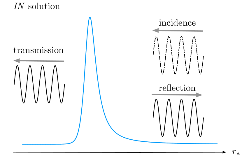
(a) IN solution

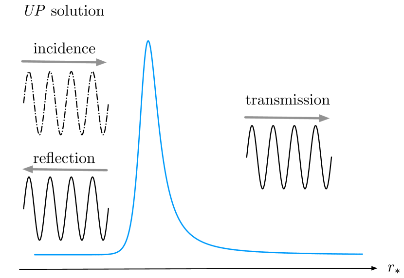
(b) UP solution

Figure 1: Physical interpretations of the amplitudes in front of each of the asymptotic solutions, for the IN solution (upper panel) and for the UP solution (lower panel).

In numerical computations, however, instead of starting with an incident wave, it is easier to start with a transmitted wave, and then integrate outward (inward) for $R^{\mathrm{in}}$ ($R^{\mathrm{up}}$) to extract the corresponding incidence and reflection amplitude at infinity (at the horizon). Inspecting Eq. (29) and (30), we can see why it is challenging to accurately read off those amplitudes if one solves the Teukolsky equation numerically using Eq. (3) directly as the amplitude of the incident and the reflected wave are of different orders of magnitude. For the $R^{\mathrm{in}}$ solution as $r\to\infty$, the ratio of the amplitude of the right-going wave to that of the left-going wave is $\sim 1/r^{2s}$ (which becomes infinitely-large for $s<0$ and infinitely-small for $s>0$). While for the $R^{\mathrm{up}}$ solution as $r\to r_{+}$, that ratio is $\sim\Delta^{s}$ (which again becomes infinitely-large for $s<0$ and infinitely-small for $s>0$ as $\Delta\to 0$ when $r\to r_{+}$). This implies that when solving Eq. (3) numerically with a finite precision, the numerical solution will be completely dominated by the right-going wave and thus impossible to extract the amplitude for the left-going wave.

To see that $R^{\mathrm{in}}$ and $R^{\mathrm{up}}$ are indeed linearly independent, we can calculate the scaled Wronskian $\mathcal{W}_{R}$ of the two solutions, which is given by

$$\mathcal{W}_{R}=\Delta^{s+1}\left(R^{\mathrm{in}}{R^{\mathrm{up}}}^{\prime}-R^{\mathrm{up}}{R^{\mathrm{in}}}^{\prime}\right).$$ (31)

Substituting the asymptotic forms of the two solutions $R^{\mathrm{in,up}}$ in Eq. (29) and (30) respectively when $r\to\infty$ gives the relation

$$\mathcal{W}_{R}=2i\omega C^{\mathrm{trans}}_{\mathrm{T}}B^{\mathrm{inc}}_{\mathrm{T}},$$ (32)

which is a non-zero constant (when $\omega\neq 0$) and thus they are indeed linearly independent. If instead we substitute the asymptotic forms of $R^{\mathrm{in,up}}$ when $r\to r_{+}$ into Eq. (31), we obtain another relation for $\mathcal{W}_{R}$, which is

$$\mathcal{W}_{R}=\left[2ip(r_{+}^{2}+a^{2})+2s(r_{+}-1)\right]B^{\mathrm{trans}}_{\mathrm{T}}C^{\mathrm{inc}}_{\mathrm{T}}.$$ (33)

By equating Eq. (32) and Eq. (33), we get an identity relating $(B^{\mathrm{inc}}_{\mathrm{T}}/B^{\mathrm{trans}}_{\mathrm{T}})$ with $(C^{\mathrm{inc}}_{\mathrm{T}}/C^{\mathrm{trans}}_{\mathrm{T}})$. From a numerical standpoint, we can use this identity as a sanity check of numerical solutions. More explicitly, the identity is given by

$$\dfrac{B^{\mathrm{inc}}_{\mathrm{T}}}{B^{\mathrm{trans}}_{\mathrm{T}}}=\dfrac{p(r_{+}^{2}+a^{2})-is(r_{+}-1)}{\omega}\dfrac{C^{\mathrm{inc}}_{\mathrm{T}}}{C^{\mathrm{trans}}_{\mathrm{T}}}.$$ (34)

It also means that we technically only need to read off $\left\{B^{\mathrm{ref}}_{\mathrm{T}},B^{\mathrm{inc}}_{\mathrm{T}},C^{\mathrm{ref}}_{\mathrm{T}}\right\}$ or $\left\{B^{\mathrm{ref}}_{\mathrm{T}},C^{\mathrm{ref}}_{\mathrm{T}},C^{\mathrm{inc}}_{\mathrm{T}}\right\}$ from numerical solutions since the rest of the amplitudes are either fixed by the normalization convention (which will be covered shortly below), or by the constant scaled Wronskian which can be computed at an arbitrary location within the domain of the numerical solutions.

II.2.2 Generalized Sasaki-Nakamura equation

Now we turn to the GSN equation. Suppose the GSN transformation is of the form of Eq. (25) and satisfies Eq. (27), the GSN potentials $\mathcal{F}(r)$ and $\mathcal{U}(r)$ then have the following asymptotic behaviors (see Fig. 2 for a visualization)

$$\mathcal{F}(r)\sim\begin{cases}0+\mathcal{O}(r-r_{+})&r\to r_{+}\\ \dfrac{-c_{1}/c_{0}}{r^{2}}+\mathcal{O}(r^{-3})&r\to\infty\\ \end{cases},$$ (35)

$$\mathcal{U}(r)\sim\begin{cases}-p^{2}+\mathcal{O}(r-r_{+})&r\to r_{+}\\ -\omega^{2}+\mathcal{O}(r^{-2})&r\to\infty\\ \end{cases}.$$ (36)

To see more clearly that the GSN potentials are indeed short-ranged, we re-cast the GSN equation into the same form as Eq. (6) by writing $Y\equiv X/\sqrt{\eta}$. Fig. 3 shows the magnitude of the potential $V_{Y}(r)$ associated to the Teukolsky equation (blue) and the GSN equation (orange) respectively. Specifically we are showing the potentials of the $s=-2,\ell=2,m=2$ mode with $a=0.7$ and $\omega=1$ as examples. We can see that the potential for the Teukolsky equation decays only at $1/r$ when $r\to\infty$ (and hence long-ranged) while the potential for the GSN equation decays at $1/r^{2}$ when $r\to\infty$ (and hence short-ranged).

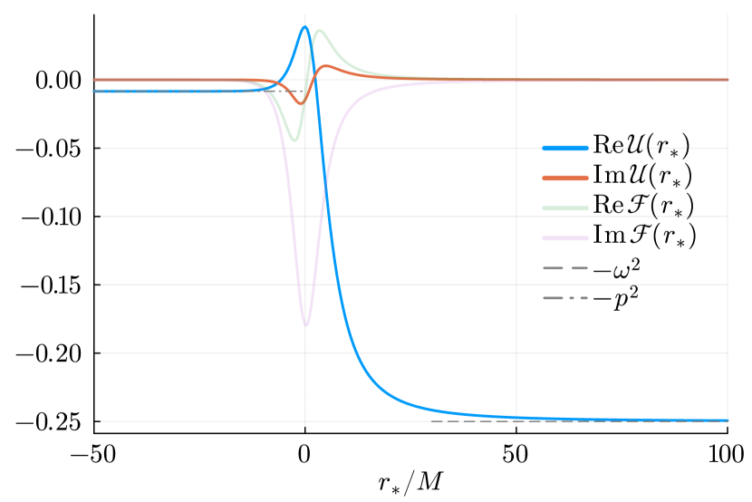
Figure 2: Asymptotic behaviors of the GSN potentials $\mathcal{F}(r)$ and $\mathcal{U}(r)$. Both potentials quickly approach to their corresponding asymptotic values. In particular, $\mathcal{U}(r)$ approaches to $-p^{2}$ near the horizon and $-\omega^{2}$ near infinity respectively.

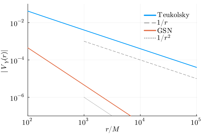
Figure 3: Potential $V_{Y}(r)$ associated to the Teukolsky equation and the GSN equation. As $r\to\infty$, the potential for the Teukolsky equation decays at $1/r$ and thus it is long-ranged, while the potential for the GSN equation decays at a steeper $1/r^{2}$ and hence it is short-ranged.

The asymptotic behaviors of the GSN potentials imply that as $r\to r_{+}$, the GSN equation behaves like a simple wave equation $d^{2}X/dr_{*}^{2}+p^{2}X=0$, admitting simple plane-wave solutions $e^{\pm ipr_{*}}$. Similarly when $r\to\infty$, the GSN equation behaves like $d^{2}X/dr_{*}^{2}+\omega^{2}X=0$, again admitting plane-wave solutions $e^{\pm i\omega r_{*}}$. Therefore, we can similarly construct the pair of linearly-independent solutions $\left\{X^{\mathrm{in}},X^{\mathrm{up}}\right\}$ that satisfies the purely-ingoing boundary condition at the horizon and the purely-outgoing boundary condition at infinity respectively using these asymptotic solutions. Mathematically,

$$X^{\mathrm{in}}(r_{*}) =\begin{cases}B^{\mathrm{trans}}_{\mathrm{SN}}e^{-ipr_{*}}&r_{*}\to-\infty\\ B^{\mathrm{inc}}_{\mathrm{SN}}e^{-i\omega r_{*}}+B^{\mathrm{ref}}_{\mathrm{SN}}e^{i\omega r_{*}}&r_{*}\to\infty\\ \end{cases},$$ (37)

$$X^{\mathrm{up}}(r_{*}) =\begin{cases}C^{\mathrm{ref}}_{\mathrm{SN}}e^{-ipr_{*}}+C^{\mathrm{inc}}_{\mathrm{SN}}e^{ipr_{*}}&r_{*}\to-\infty\\ C^{\mathrm{trans}}_{\mathrm{SN}}e^{i\omega r_{*}}&r_{*}\to\infty\end{cases}.$$ (38)

Here the amplitudes in front of each of the asymptotic solutions have the same physical interpretations as in Eq. (29) and (30) (c.f. Fig. 1). Again by inspecting Eq. (37) and (38), we can see that it is easy to accurately read off those amplitudes as the ratio of the asymptotic amplitude of the incident wave to that of the reflected wave at both boundaries is $\sim\mathcal{O}(1)$, instead of being infinitely-large or infinitely-small in the Teukolsky formalism.

Similar to the case of Teukolsky functions, we can also define a scaled Wronskian $\mathcal{W}_{X}$ for the GSN functions, namely

$$\mathcal{W}_{X}=\dfrac{1}{\eta}\left[X^{\mathrm{in}}(dX^{\mathrm{up}}/dr_{*})-(dX^{\mathrm{in}}/dr_{*})X^{\mathrm{up}}\right],$$ (39)

which is also a constant. Substituting the asymptotic forms of $X^{\mathrm{in,up}}$ in Eq. (37) and (38) respectively as $r_{*}\to\infty$, and the fact that $\eta(r)\to c_{0}$ as $r\to\infty$, it can be shown that

$$\mathcal{W}_{X}=\dfrac{2i\omega C^{\mathrm{trans}}_{\mathrm{SN}}B^{\mathrm{inc}}_{\mathrm{SN}}}{c_{0}}.$$ (40)

Equivalently, we can also use the asymptotic forms of $X^{\mathrm{in,up}}$ as $r_{*}\to-\infty$, and the fact that $\eta(r\to r_{+})\sim\mathcal{O}(1)$ to show that

$$\mathcal{W}_{X}=\dfrac{2ipB^{\mathrm{trans}}_{\mathrm{SN}}C^{\mathrm{inc}}_{\mathrm{SN}}}{\eta(r_{+})},$$ (41)

We can again equate Eq. (40) and Eq. (41) to get an identity relating $B^{\mathrm{inc}}_{\mathrm{SN}}/B^{\mathrm{trans}}_{\mathrm{SN}}$ with $C^{\mathrm{inc}}_{\mathrm{SN}}/C^{\mathrm{trans}}_{\mathrm{SN}}$ to check the sanity of numerical solutions. Explicitly, the identity is given by

$$\dfrac{B^{\mathrm{inc}}_{\mathrm{SN}}}{B^{\mathrm{trans}}_{\mathrm{SN}}}=\dfrac{pc_{0}}{\omega\eta(r_{+})}\dfrac{C^{\mathrm{inc}}_{\mathrm{SN}}}{C^{\mathrm{trans}}_{\mathrm{SN}}}.$$ (42)

An interesting and useful relation between the scaled Wronskians for GSN functions $\mathcal{W}_{X}$ and that for Teukolsky functions $\mathcal{W}_{R}$ (with the same $s,\ell,m,a,\omega$) is that despite having different definitions (see Eq. (31) for $\mathcal{W}_{R}$ and Eq. (39) for $\mathcal{W}_{X}$), they are actually identical, i.e.

$$\mathcal{W}_{X}=\mathcal{W}_{R},$$ (43)

where we give a derivation in App. C. This means that GSN transformations (not limited only to our particular choices of $g_{i}$) are scaled-Wronskian-preserving. This also means that one can compute the QNM spectra of Kerr BHs using either the Teukolsky formalism or the GSN formalism (see Sec. IV.2).

Since one can freely rescale a homogeneous solution by a constant factor, we use this freedom to set $B^{\mathrm{trans}}_{\mathrm{SN}}=C^{\mathrm{trans}}_{\mathrm{SN}}=1$, i.e. we normalize our solutions to the GSN equation to have a unit SN transmission amplitude. However, the common normalization convention in literature is to normalize $R^{\mathrm{in}}(r)$ and $R^{\mathrm{up}}(r)$ to each have a unit transmission amplitude, i.e. $B^{\mathrm{trans}}_{\mathrm{T}}=C^{\mathrm{trans}}_{\mathrm{T}}=1$. In fact, one can relate incidence/reflection/transmission amplitudes in the GSN formalism to that in the Teukolsky formalism and vice versa by frequency-dependent conversion factors. To see why this is the case and to obtain the conversion factors, note that when going from a Teukolsky function to the corresponding GSN function, we have the ${}_{s}\Lambda$ operator that satisfies

$${}_{s}\Lambda\left[f(r)e^{\pm ikr_{*}}\right]\propto e^{\pm ikr_{*}},$$ (44)

and vice versa with the inverse operator ${}_{s}\Lambda^{-1}$ that satisfies

$${}_{s}\Lambda^{-1}\left[f(r)e^{\pm ikr_{*}}\right]\propto e^{\pm ikr_{*}},$$ (45)

for any differentiable function $f(r)$ and $k$ is any non-zero constant, since both ${}_{s}\Lambda$ and ${}_{s}\Lambda^{-1}$ are linear differential operators. This means that we can simply match the asymptotic solution in one formalism with the corresponding asymptotic solution with the same exponential dependence in another formalism transformed by either ${}_{s}\Lambda$ or ${}_{s}\Lambda^{-1}$ at the appropriate boundary.

For example, to get the conversion factor $C^{\mathrm{trans}}_{\mathrm{T}}/C^{\mathrm{trans}}_{\mathrm{SN}}$, we match the asymptotic solution as $r\to\infty$ for the Teukolsky and the GSN formalism like

$$C^{\mathrm{trans}}_{\mathrm{SN}}\left[1+\mathcal{O}\left(\dfrac{1}{r}\right)\right]e^{i\omega r_{*}}=\\ C^{\mathrm{trans}}_{\mathrm{T}}{}_{s}\Lambda\left\{\dfrac{1}{r^{2s+1}}\left[1+\mathcal{O}\left(\dfrac{1}{r}\right)\right]e^{i\omega r_{*}}\right\},$$ (46)

where the expression on the RHS, to the leading order, should be $\sim\mathcal{O}\left(1\right)e^{i\omega r_{*}}$. We can then obtain the desired conversion factor by taking the limit as

$$\dfrac{C^{\mathrm{trans}}_{\mathrm{SN}}}{C^{\mathrm{trans}}_{\mathrm{T}}}=\lim_{r\to\infty}{}_{s}\Lambda\left\{\dfrac{1}{r^{2s+1}}\left[1+\mathcal{O}\left(\dfrac{1}{r}\right)\right]e^{i\omega r_{*}}\right\}e^{-i\omega r_{*}},$$ (47)

and we know that the expression on the RHS does not depend on $e^{\pm i\omega r_{*}}$ using Eq. (44) so that the limit could be determinate. Equivalently, we can also match the asymptotic solution as $r\to\infty$ in the two formalism like this instead

$$C^{\mathrm{trans}}_{\mathrm{T}}\dfrac{1}{r^{2s+1}}\left[1+\mathcal{O}\left(\dfrac{1}{r}\right)\right]e^{i\omega r_{*}}=\\ C^{\mathrm{trans}}_{\mathrm{SN}}{}_{s}\Lambda^{-1}\left\{\left[1+\mathcal{O}\left(\dfrac{1}{r}\right)\right]e^{i\omega r_{*}}\right\},$$ (48)

where the expression on the RHS, to the leading order, should be $\sim\mathcal{O}\left(1\right)r^{-\left(2s+1\right)}e^{i\omega r_{*}}$. Similarly we can obtain

$$\dfrac{C^{\mathrm{trans}}_{\mathrm{T}}}{C^{\mathrm{trans}}_{\mathrm{SN}}}=\lim_{r\to\infty}{}_{s}\Lambda^{-1}\left\{\left[1+\mathcal{O}\left(\dfrac{1}{r}\right)\right]e^{i\omega r_{*}}\right\}r^{2s+1}e^{-i\omega r_{*}},$$ (49)

and again we know that the RHS of the expression does not depend on $e^{\pm i\omega r_{*}}$ using Eq. (45) so that the limit could be determinate.

We find that sometimes it is more convenient to compute the limit in the form of Eq. (47) than to use the limit in the form of Eq. (49) in order to find the same conversion factor, and in some cases the reverse is true even though formally both expressions should give the same answer. In fact, using the identity between the scaled Wronskian of the GSN functions $\mathcal{W}_{X}$ and that of the Teukolsky functions $\mathcal{W}_{R}$, we can simplify expressions for these conversion factors by equating expressions of $\mathcal{W}_{X}$ in terms of the incidence and transmission amplitudes in the GSN formalism with expressions of $\mathcal{W}_{R}$ in terms of those amplitudes in the Teukolsky formalism. In particular, we get identities relating these conversion factors as

$$\dfrac{C^{\mathrm{trans}}_{\mathrm{T}}}{C^{\mathrm{trans}}_{\mathrm{SN}}}\dfrac{B^{\mathrm{inc}}_{\mathrm{T}}}{B^{\mathrm{inc}}_{\mathrm{SN}}} =\dfrac{1}{c_{0}},$$ (50)

$$\dfrac{B^{\mathrm{trans}}_{\mathrm{T}}}{B^{\mathrm{trans}}_{\mathrm{SN}}}\dfrac{C^{\mathrm{inc}}_{\mathrm{T}}}{C^{\mathrm{inc}}_{\mathrm{SN}}} =\dfrac{2ip}{\eta(r_{+})\left[2ip(r_{+}^{2}+a^{2})+2s(r_{+}-1)\right]}.$$ (51)

These identities imply that we only need to derive either $\dfrac{C^{\mathrm{trans}}_{\mathrm{T}}}{C^{\mathrm{trans}}_{\mathrm{SN}}}$ or $\dfrac{B^{\mathrm{inc}}_{\mathrm{T}}}{B^{\mathrm{inc}}_{\mathrm{SN}}}$ and either $\dfrac{B^{\mathrm{trans}}_{\mathrm{T}}}{B^{\mathrm{trans}}_{\mathrm{SN}}}$ or $\dfrac{C^{\mathrm{inc}}_{\mathrm{T}}}{C^{\mathrm{inc}}_{\mathrm{SN}}}$.

II.2.3 Higher-order corrections to asymptotic behaviors

In Eq. (37) and (38), we use the asymptotic solutions of the GSN equation only to their leading order (i.e. $\mathcal{O}(r^{0})$). However, in order to obtain accurate numerical solutions solved on a numerically-finite interval (e.g. $\left[r^{\mathrm{in}}_{*},r^{\mathrm{out}}_{*}\right]$), it is more efficient to include higher-order corrections to the asymptotic solutions than to simply set $r^{\mathrm{in}}_{*}$ as a small number and $r^{\mathrm{out}}_{*}$ as a large number. To find such higher-order corrections, we use an ansatz of the form

$$X(r_{*})\sim\begin{cases}f^{\infty}_{\pm}(r)e^{\pm i\omega r_{*}},&r_{*}\to\infty\\ g^{\mathrm{H}}_{\pm}(r)e^{\pm ipr_{*}},&r_{*}\to-\infty\end{cases},$$ (52)

where the plus (minus) sign corresponds to the out/right-going (in/left-going) mode, and the superscript $\infty$ ($\mathrm{H}$) corresponds to the outer (inner) boundary at infinity (the horizon). Substituting Eq. (52) back to the GSN equation in Eq. (22), we get four second-order ODEs for each of the functions $f^{\infty}_{\pm}(r)$ and $g^{\mathrm{H}}_{\pm}(r)$ (c.f. Eq. (95)). We look for their formal series expansions of the form

$$f^{\infty}_{\pm}(r)= \sum_{j=0}^{\infty}\dfrac{\mathcal{C}^{\infty}_{\pm,j}}{\left(\omega r\right)^{j}},$$ (53)

$$g^{\mathrm{H}}_{\pm}(r)= \sum_{j=0}^{\infty}\mathcal{C}^{\mathrm{H}}_{\pm,j}\left[\omega(r-r_{+})\right]^{j},$$ (54)

where $\mathcal{C}^{\infty/\mathrm{H}}_{\pm,j}$ are the expansion coefficients. In App. D, we show how one can compute these coefficients using recurrence relations. Such recurrence relations for some of the spin weights ($s=0$ and $s=-2$) can also be found in literature (e.g. Refs. [38, 39, 40]). In App. E, we show explicitly the expressions of the expansion coefficients $\mathcal{C}^{\infty}_{\pm,j}$ for $j=0,1,2,3$.

With the explicit GSN transformation and hence the GSN potentials and the GSN equation as discussed in Sec. II.1, as well as the asymptotic solutions to the GSN equation and the conversion factors for converting asymptotic amplitudes between the Teukolsky and the GSN formalism as discussed in Sec. II.2, we now have all the necessary ingredients to use the GSN formalism to perform numerical computations. In the next section, we describe the recipes to use those ingredients to get homogenous solutions to both the Teukolsky and the GSN equation.

III Numerical implementation

In principle, a frequency-domain Teukolsky/GSN equation solver can be implemented in any programming language with the help of the ingredients in Sec. II and App. E. Here we describe an open-source implementation of the GSN formalism that is written in julia [35], namely GeneralizedSasakiNakamura.jl. Instead of fixing a particular choice of an numerical integrator for solving Eq. (22), the code can be used in conjunction with other julia packages, such as DifferentialEquations.jl [41], which implements a suite of ODE solvers. The GSN potentials $\mathcal{F}(r),\mathcal{U}(r)$ for $s=0,\pm 1,\pm 2$ are implemented as pure functions in julia, and can be evaluated to arbitrary precision. This also allows us to use automatic differentiation (AD) to compute corrections to the asymptotic boundary conditions at arbitrary order (see App. D).

III.1 Numerical solutions to the Generalized Sasaki-Nakamura equation

III.1.1 Rewriting Generalized Sasaki-Nakamura functions as complex phase functions

Instead of solving directly for the GSN function $X(r_{*})$, we follow Ref. [44] and introduce a complex phase function $\Phi(r_{*})$ such that

$$X(r_{*})\equiv\exp\left[i\Phi\left(r_{*}\right)\right].$$ (55)

Substituting Eq. (55) into Eq. (22), we obtain a first-order non-linear differential equation as

$$\dfrac{d}{dr_{*}}\left(\dfrac{d\Phi}{dr_{*}}\right)=-i\,\mathcal{U}+\mathcal{F}\left(\dfrac{d\Phi}{dr_{*}}\right)-i\left(\dfrac{d\Phi}{dr_{*}}\right)^{2}.$$ (56)

Such a differential equation is also known as a Riccati equation. Furthermore, the conversion between $\left(X,dX/dr_{*}\right)$ and $\left(\Phi,d\Phi/dr_{*}\right)$ is given by

$$\Phi =-i\log\left(X\right),$$ (57)

$$\dfrac{d\Phi}{dr_{*}} =-i\dfrac{dX/dr_{*}}{X}.$$ (58)

While at first glance it may seem unwise to turn a linear problem into a non-linear problem, solving Eq. (56) numerically presents no additional challenge compared to solving directly Eq. (22). In fact, there are advantages in writing the GSN function in the form of Eq. (55), especially when $|\omega|$ is large. Recall that asymptotically (both near infinity and near the horizon) GSN functions behave like plane waves, i.e. $X$ oscillates like $\exp\left(\pm ikr_{*}\right)$ where $|k|$ is the oscillation frequency (assuming $k$ is real, and recall that $|k|\to|\omega|$ when $r_{*}\to\infty$ and $|k|\to|p|$ when $r_{*}\to-\infty$). Therefore, in order to properly resolve the oscillations, the step size $\delta r_{*}$ for the numerical integrator needs to be much less than the wavelength, i.e. $\delta r_{*}\ll 1/|k|$. This can get quite small for large $|k|$, which results in taking a longer time to integrate Eq. (22) for a fixed accuracy.

Fortunately this is not the case when solving for the complex phase function $\Phi(r_{*})$ since it is varying much slower (spatially) than the GSN function $X(r_{*})$. Intuitively this is because the complex exponential in Eq. (55) accounts for most of the oscillatory behaviors. This is especially true if we consider the asymptotic plane-wave-like solutions of the GSN equation, where the real part of the phase function $\Phi_{\mathrm{Re}}(r_{*})\sim kr_{*}$ is linear in $r_{*}$, and the imaginary part of the phase function $\Phi_{\mathrm{Im}}(r_{*})$ is constant in $r_{*}$.

However, this might not be the case when we consider general solutions to the GSN equation where the left-going and the right-going modes are superimposed, for example the $X^{\mathrm{in,up}}$ pair as shown in Eq. (37) and Eq. (38). That being said, the variation of the complex phase function due to the beating or interference between the left-/right-going modes depends on their relative amplitude (which is in general a complex number and hence introduces a phase shift). In particular, physically Kerr BHs are much more permeable to waves at high frequencies (see Fig. 6). This means that at those high frequencies, the relative amplitudes of the left-/right-going modes are going to be extreme and hence the beating will be suppressed.

III.1.2 Solving $X^{\mathrm{in,up}}$ as initial value problems

Recall that there is a pair of linearly-independent solutions to the GSN equation that is of particular interest, namely $\left\{X^{\mathrm{in}},X^{\mathrm{up}}\right\}$, where $X^{\mathrm{in}}$ satisfies the boundary condition that it is purely in-going at the horizon as given by Eq. (37), and $X^{\mathrm{up}}$ satisfies the boundary condition that it is purely out-going at infinity as given by Eq. (38), respectively.

Despite the usage of the term “boundary condition”, what we are really enforcing is the asymptotic form of a solution at one of the two boundaries, $X^{\mathrm{in}}$ at the horizon and $X^{\mathrm{up}}$ at infinity respectively. This can be formulated as an initial value problem. Explicitly for $\hat{X}^{\mathrm{in}}$, where a hat denotes a numerical solution hereafter, we integrate Eq. (56) outwards from the (finite) inner boundary $r_{*}^{\mathrm{in}}$ to the (finite) outer boundary $r_{*}^{\mathrm{out}}$ with

$$\hat{X}(r^{\mathrm{in}}_{*}) =g^{\mathrm{H}}_{-}\left(r(r^{\mathrm{in}}_{*})\right)e^{-ipr^{\mathrm{in}}_{*}},$$ (59)

$$\dfrac{d\hat{X}(r^{\mathrm{in}}_{*})}{dr_{*}} =-ip\hat{X}(r^{\mathrm{in}}_{*})+\left.\dfrac{dr}{dr_{*}}\dfrac{dg^{\mathrm{H}}_{-}(r)}{dr}\right|_{r=r(r^{\mathrm{in}}_{*})}e^{-ipr^{\mathrm{in}}_{*}},$$ (60)

as the initial values at $r_{*}=r_{*}^{\mathrm{in}}$ after converting them to $\hat{\Phi}^{\mathrm{in}}$ and $d\hat{\Phi}^{\mathrm{in}}/dr_{*}$ using Eq. (57) and Eq. (58) respectively. Similarly for $\hat{X}^{\mathrm{up}}$, we integrate Eq. (56) inwards from the outer boundary $r_{*}^{\mathrm{out}}$ to the inner boundary $r_{*}^{\mathrm{in}}$ with

$$\hat{X}(r^{\mathrm{out}}_{*}) =f^{\infty}_{+}\left(r(r^{\mathrm{out}}_{*})\right)e^{i\omega r^{\mathrm{out}}_{*}},$$ (61)

$$\dfrac{d\hat{X}(r^{\mathrm{out}}_{*})}{dr_{*}} =i\omega\hat{X}(r^{\mathrm{out}}_{*})+\left.\dfrac{dr}{dr_{*}}\dfrac{df^{\infty}_{+}(r)}{dr}\right|_{r=r(r^{\mathrm{out}}_{*})}e^{i\omega r^{\mathrm{out}}_{*}},$$ (62)

as the initial values at $r_{*}=r_{*}^{\mathrm{out}}$ after converting them to $\hat{\Phi}^{\mathrm{up}}$ and $d\hat{\Phi}^{\mathrm{up}}/dr_{*}$ using again Eq. (57) and Eq. (58) respectively. Note that for both $\hat{X}^{\mathrm{in}}$ and $\hat{X}^{\mathrm{up}}$, we have chosen the normalization convention of a unit transmission amplitude, i.e. $B^{\mathrm{trans}}_{\mathrm{SN}}=C^{\mathrm{trans}}_{\mathrm{SN}}=1$. After solving Eq. (56) numerically for a complex phase function $\hat{\Phi}(r_{*})$ and its derivative $d\hat{\Phi}/dr_{*}$ on a grid of $r_{*}\in[r_{*}^{\mathrm{in}},r_{*}^{\mathrm{out}}]$, we first convert them back to $\hat{X}$ and $d\hat{X}/dr_{*}$ using Eq. (55) and Eq. (58) respectively.

III.1.3 Transforming Generalized Sasaki-Nakamura functions to Teukolsky functions

In principle, if we want to transform a GSN function $\hat{X}$ back to a Teukolsky function, we simply need to apply the inverse operator ${}_{s}\Lambda^{-1}$ on the numerical GSN function. Since we have the numerical solutions to both $\hat{X}$ and $d\hat{X}/dr_{*}$, the inverse operator can actually be written as a matrix multiplication to the column vector $\left(\hat{X},d\hat{X}/dr_{*}\right)^{T}$.

First, consider the conversion from $\left(\hat{X},d\hat{X}/dr_{*}\right)^{T}$ to $\left(\hat{X},\hat{X}^{\prime}\right)^{T}$. This can be done by left-multiplying the column vector with the matrix

$$M_{1}=\begin{pmatrix}1&0\\ 0&\dfrac{r^{2}+a^{2}}{\Delta}\end{pmatrix}.$$ (63)

Next, consider the transformation from $\left(\hat{X},\hat{X}^{\prime}\right)^{T}$ to $\left(\hat{\chi},\hat{\chi}^{\prime}\right)^{T}$ using Eq. (13). Again this can be done by left-multiplying the column vector $\left(\hat{X},\hat{X}^{\prime}\right)^{T}$ by the matrix

$$M_{2}=\begin{pmatrix}\dfrac{1}{\sqrt{\left(r^{2}+a^{2}\right)\Delta^{s}}}&0\\ \left(\dfrac{1}{\sqrt{\left(r^{2}+a^{2}\right)\Delta^{s}}}\right)^{\prime}&\dfrac{1}{\sqrt{\left(r^{2}+a^{2}\right)\Delta^{s}}}\end{pmatrix}.$$ (64)

At last, the transformation from $\left(\hat{\chi},\hat{\chi}^{\prime}\right)^{T}$ to $\left(R,R^{\prime}\right)^{T}$ is given by the matrix equation as shown in Eq. (11), where we now explicitly define the matrix as

$$M_{3}=\dfrac{1}{\eta}\begin{pmatrix}\alpha+\beta^{\prime}\Delta^{s+1}&-\beta\Delta^{s+1}\\ -(\alpha^{\prime}+\beta V_{\mathrm{T}}\Delta^{s})&\alpha\\ \end{pmatrix}.$$ (65)

The overall transformation from $\hat{X}$ and $d\hat{X}/dr_{*}$ to $R$ and $R^{\prime}$ is thus given by the matrix equation

$$\begin{pmatrix}\hat{R}\\ \hat{R}^{\prime}\end{pmatrix}=M_{3}M_{2}M_{1}\begin{pmatrix}\hat{X}\\ \dfrac{d\hat{X}}{dr_{*}}\end{pmatrix}.$$ (66)

By multiplying $\left(\hat{X},d\hat{X}/dr_{*}\right)^{T}$ with the overall transformation matrix $M_{3}M_{2}M_{1}$ that we explicitly simplified in order to facilitate cancellations between terms. This allows us to accurately convert numerical GSN functions to Teukolsky functions close to the horizon ($\Delta\to 0$) when some of the terms, such as $\alpha(r)$, diverge near the horizon.

III.2 Extracting incidence and reflection amplitudes from numerical solutions

Apart from evaluating a GSN or a Teukolsky function numerically on a grid of $r$- or $r_{*}$-coordinates, it is also useful to be able to determine the incidence and the reflection amplitude at a particular frequency $\omega$ (see Sec. II.2 for a theoretical discussion) from a numerical solution accurately. This is essential for constructing inhomogeneous solutions using the Green’s function method (e.g. calculating gravitational waveforms observed at infinity) and for scattering problems (e.g. calculating the greybody factor of a BH as a function of the wave frequency $\omega$).

Since we only have numerical solutions on a finite grid of $r_{*}\in[r_{*}^{\mathrm{in}},r_{*}^{\mathrm{out}}]$, in order to determine the reflection amplitude $\hat{B}^{\mathrm{ref}}_{\mathrm{SN}}$ and the incidence amplitude $\hat{B}^{\mathrm{inc}}_{\mathrm{SN}}$ of a $\hat{X}^{\mathrm{in}}$ solution in the GSN formalism we solve the system of linear equations at the outer boundary $r_{*}^{\mathrm{out}}$ that

$$\left.\begin{pmatrix}f^{\infty}_{+}(r)e^{i\omega r_{*}}&f^{\infty}_{-}(r)e^{-i\omega r_{*}}\\[10.00002pt] (df^{\infty}_{+}/dr_{*}+i\omega f^{\infty}_{+})e^{i\omega r_{*}}&(df^{\infty}_{-}/dr_{*}-i\omega f^{\infty}_{-})e^{-i\omega r_{*}}\end{pmatrix}\right|_{r^{\mathrm{out}}_{*}}$$ (67)

$$\times\begin{pmatrix}\hat{B}^{\mathrm{ref}}_{\mathrm{SN}}\\[10.00002pt] \hat{B}^{\mathrm{inc}}_{\mathrm{SN}}\end{pmatrix}=\left.\begin{pmatrix}\hat{X}^{\mathrm{in}}\\ \dfrac{d\hat{X}^{\mathrm{in}}}{dr_{*}}\end{pmatrix}\right|_{r^{\mathrm{out}}_{*}},$$

where we impose continuity of the numerical solution $(\hat{X}^{\mathrm{in}},d\hat{X}^{\mathrm{in}}/dr_{*})$ with the analytical asymptotic solution near infinity at $r_{*}=r_{*}^{\mathrm{out}}$. Similarly, we use the same scheme to determine the reflection amplitude $\hat{C}^{\mathrm{ref}}_{\mathrm{SN}}$ and the incidence amplitude $\hat{C}^{\mathrm{inc}}_{\mathrm{SN}}$ of a $\hat{X}^{\mathrm{up}}$ solution in the GSN formalism at the inner boundary $r_{*}^{\mathrm{in}}$ by solving

$$\left.\begin{pmatrix}g^{\mathrm{H}}_{+}(r)e^{ipr_{*}}&g^{\mathrm{H}}_{-}(r)e^{-ipr_{*}}\\[10.00002pt] (dg^{\mathrm{H}}_{+}/dr_{*}+ipg^{\mathrm{H}}_{+})e^{ipr_{*}}&(dg^{\mathrm{H}}_{-}/dr_{*}-ipg^{\mathrm{H}}_{-})e^{-ipr_{*}}\end{pmatrix}\right|_{r^{\mathrm{in}}_{*}}$$ (68)

$$\times\begin{pmatrix}\hat{C}^{\mathrm{inc}}_{\mathrm{SN}}\\[10.00002pt] \hat{C}^{\mathrm{ref}}_{\mathrm{SN}}\end{pmatrix}=\left.\begin{pmatrix}\hat{X}^{\mathrm{up}}\\ \dfrac{d\hat{X}^{\mathrm{up}}}{dr_{*}}\end{pmatrix}\right|_{r^{\mathrm{in}}_{*}},$$

where again we impose continuity of the numerical solution $(\hat{X}^{\mathrm{up}},d\hat{X}^{\mathrm{up}}/dr_{*})$ to the asymptotic solution near the horizon at $r_{*}=r_{*}^{\mathrm{in}}$.

Indeed, the inclusion of the higher-order corrections $f^{\infty}_{\pm}$ at the outer boundary and $g^{\mathrm{H}}_{\pm}$ at the inner boundary respectively allow us to get very good agreements on the incidence and the reflection amplitudes over a range of frequencies with the MST method, which we will show in the next sub-section.

III.3 Numerical results

Here we showcase some numerical results obtained using our GeneralizedSasakiNakamura.jl implementation. Unless otherwise specified, we use the ODE solver Vern9 [45] as implemented in DifferentialEquations.jl [41], and we include corrections to the asymptotic solutions at infinity up to the third order (i.e. truncating the sum in Eq. (53) at $j=3$) and that at the horizon only to the zeroth order (i.e. taking only the leading term $j=0$ in the sum in Eq. (54)). We set the numerical inner boundary at $r_{*}^{\mathrm{in}}=-50M$ and the outer boundary at $r_{*}^{\mathrm{out}}=1000M$. We use double-precision floating-point numbers throughout, and both the “absolute tolerance” abstol (roughly the error around the zero point) and the “relative tolerance” reltol (roughly the local error) passed to the numerical ODE solver are set to $10^{-12}$.

III.3.1 Numerical solutions

Fig. 4 shows the IN solution in the GSN formalism of the $s=-2,\ell=2,m=2$ mode for a BH with $a/M=0.7$ and two different values of $\omega$, in terms of the GSN function $X$ and the complex frequency function $d\Phi/dr_{*}$. Recall that for an IN solution, it is purely in-going at the horizon. We see from the figure that for both $M\omega=0.5$ (upper panel) and $M\omega=1$ (lower panel), near the horizon, $d\hat{\Phi}/dr_{*}$ is flat and approaches to the imposed asymptotic value $-p^{2}$, while $\hat{X}$ is oscillating with the frequency $p$. On the other hand when $r_{*}\to\infty$, the IN solution is an admixture of the left- and the right-going modes where their relative amplitude, $B^{\mathrm{ref}}_{\mathrm{SN}}/B^{\mathrm{inc}}_{\mathrm{SN}}$, is $\omega$-dependent. We see from Fig. 4a that both $\hat{X}$ and $d\hat{\Phi}/dr_{*}$ exhibit oscillatory behaviors, and that the oscillation frequency for $d\hat{\Phi}/dr_{*}$ from beating is twice of that for $\hat{X}$. While we see from Fig. 4b that $\hat{X}$ is oscillatory but $d\hat{\Phi}/dr_{*}$ is flat as the ratio of the left- and right-going mode is extreme and hence beating is heavily suppressed.

This can be more easily seen in Fig. 5 where it shows the first derivative of the numerical IN solutions $d\hat{\Phi}/dr_{*}$, i.e. $d^{2}\hat{\Phi}/dr_{*}^{2}$, as indicators of how much they change locally as functions of $r_{*}$, for both the $M\omega=0.5$ and the $M\omega=1$ case. We compute the numerical derivatives using AD on the interpolant of the numerical solutions of $d\hat{\Phi}/dr_{*}$ to avoid issues with using a finite difference method. We see from the upper panel (Fig. 5a) that for $M\omega=0.5$ the oscillation in $d\hat{\Phi}/dr_{*}$ is significant, while for $M\omega=1$ we can see from the lower panel (Fig. 5b) that the oscillation is much more minute. Note that the two panels have very different scales for their $y$-axes.

Physically this boils down to the fact that the potential barriers of a Kerr BH for different types of radiation are all very permeable to waves at high frequencies. Fig. 6 shows the reflectivity of the potential barriers (for $s=0,\pm 1,\pm 2$ with $a/M=0.7$) as defined by $B^{\mathrm{ref}}_{\mathrm{SN}}/B^{\mathrm{inc}}_{\mathrm{SN}}$. This ratio compares the wave amplitude $B^{\mathrm{ref}}_{\mathrm{SN}}$ that is reflected off the potential barrier when a wave with an asymptotic amplitude $B^{\mathrm{inc}}_{\mathrm{SN}}$ is approaching the barrier from infinity. We see from Fig. 6 that the reflectivities become zero when the wave frequency gets large (while we only show for the $a/M=0.7$ case, the same is true for other values of $a/M$ as well). A low reflectivity means that the ratio of the left- and the right-going mode is going to be extreme. Explicitly for the case in Fig. 6, the right-going mode has an amplitude $|B^{\mathrm{ref}}_{\mathrm{SN}}|$ that is much smaller than the left-going mode $|B^{\mathrm{inc}}_{\mathrm{SN}}|$ when $M\omega\gtrsim 1$. The lack of beating in Fig. 4b is a manifestation of this fact.

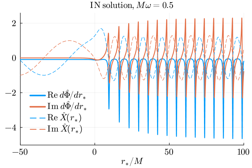
(a)

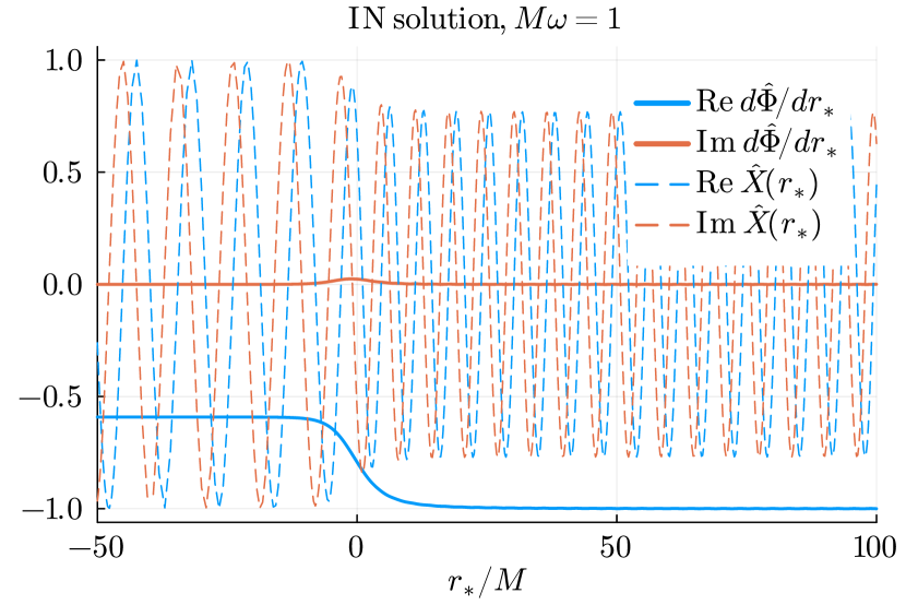
(b)

Figure 4: GSN IN solution of the $s=-2,\ell=2,m=2$ mode of a BH with $a/M=0.7$ and two different values of $\omega$ (upper panel: $M\omega=0.5$; lower panel: $M\omega=1$), in terms of the GSN function $X$ and the complex frequency function $d\Phi/dr_{*}$.

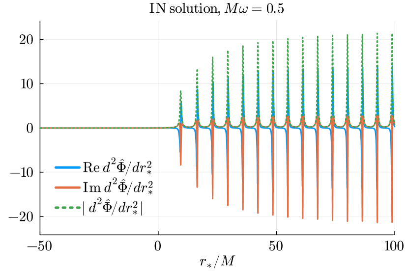
(a)

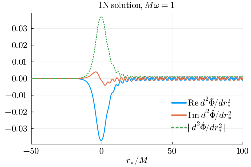
(b)

Figure 5: First derivative of the numerical solutions to the complex frequency function in Fig. 4 (i.e. $d/dr_{*}(d\hat{\Phi}/dr_{*})$), computed using AD, as indicators of how much the numerical solutions are changed locally as functions of $r_{*}$ (upper panel: $M\omega=0.5$; lower panel: $M\omega=1$).

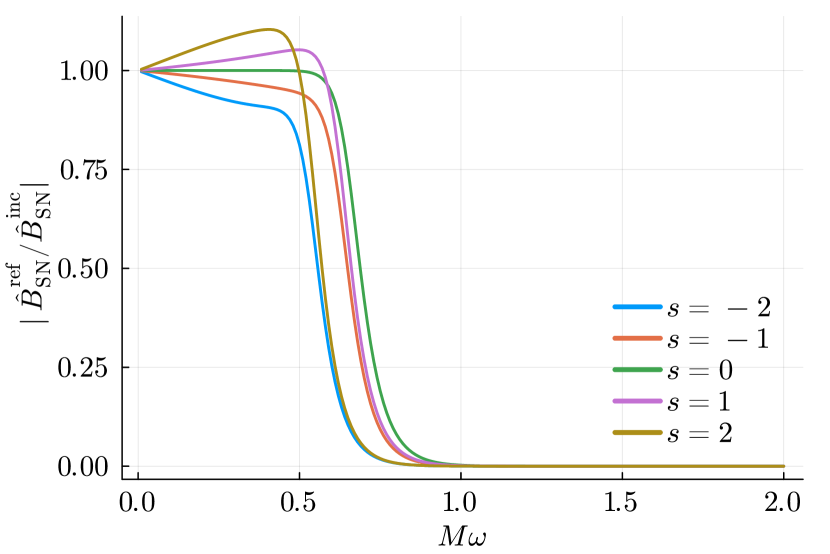
Figure 6: Reflectivity $B^{\mathrm{ref}}_{\mathrm{SN}}/B^{\mathrm{inc}}_{\mathrm{SN}}$ of a Kerr BH potential barrier in the GSN formalism. We see that for all the spin weights $s$ considered in this paper, the corresponding potential barriers are very permeable to high-frequency ($M\omega\gtrsim 1$) waves, meaning that the potentials will not reflect off the incidence waves and instead allow them to pass right through. In this figure, the BH angular momentum was set to $a/M=0.7$ but the same is true for other values of $a/M$ as well.

Fig. 7 is similar to Fig. 4 but showing the UP solution instead. Recall that for an UP solution, it is purely out-going at infinity. Again, we see from the figure that for both $M\omega=0.5$ and $M\omega=1$ (upper and lower panel respectively), $d\hat{\Phi}/dr_{*}$ is flat and approaches to the imposed asymptotic value $\omega^{2}$ as $r_{*}\to\infty$, while $\hat{X}$ is oscillating with the frequency $\omega$. Similar to the IN solutions shown in Fig. 4, since an UP solution is an admixture of the left- and the right-going modes near the horizon, depending on their relative amplitude $C^{\mathrm{ref}}_{\mathrm{SN}}/C^{\mathrm{inc}}_{\mathrm{SN}}$, both $\hat{X}$ and $d\hat{\Phi}/dr_{*}$ can be oscillatory near the horizon as shown in Fig. 7a. When the frequency $\omega$ is sufficiently high, the beating in $d\hat{\Phi}/dr_{*}$ is suppressed while $\hat{X}$ remains oscillatory as shown in Fig. 7b.

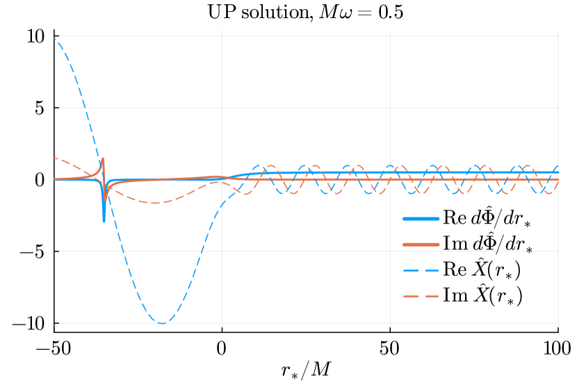
(a)

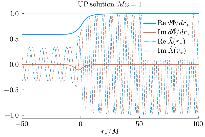
(b)

Figure 7: GSN UP solution of the $s=-2,\ell=2,m=2$ mode of a BH with $a/M=0.7$ and two different values of $\omega$ (upper panel: $M\omega=0.5$; lower panel: $M\omega=1$), in terms of the GSN function $X$ and the complex frequency function $d\Phi/dr_{*}$.

III.3.2 Numerical accuracy

As numerical solutions are only approximations to the true solutions, it is necessary to verify their accuracies. First, we need to show that the initial conditions $\hat{X}$ and $d\hat{X}/dr_{*}$ that we use are sufficiently accurate such that when solving for $\hat{X}^{\mathrm{in,up}}$ the corresponding asymptotic boundary forms are satisfied. Next, we need to show that the numerical solutions actually satisfy the GSN equation inside the integration domain. In both cases, we can evaluate the residual $\varepsilon$, which is defined as

$$\varepsilon=\left|\dfrac{d^{2}\hat{X}}{dr_{*}^{2}}-\mathcal{F}(r)\dfrac{d\hat{X}}{dr_{*}}-\mathcal{U}(r)\hat{X}\right|,$$ (69)

where a smaller value (ideally zero) means a better agreement of a numerical solution $\hat{X}$ with the GSN equation.

Fig. 8 shows the residual $\varepsilon$ of the ansatz, $f^{\infty}_{\pm}$ near infinity (upper panel) and $g^{\mathrm{H}}_{\pm}$ near the horizon (lower panel) as functions of $r_{*}$. For both panels, solid lines correspond to the out-going ansatzes and dash lines correspond to the in-going ansatzes truncated to different orders $N=0,1,2,3$, i.e. keeping the first $N+1$ terms in Eq. (53) and Eq. (54) respectively. Recall that for all the numerical results we have shown previously, we set the numerical outer boundary $r_{*}^{\mathrm{out}}=1000M$ and truncate $f^{\infty}_{\pm}$ at $N=3$ (i.e. including the first four terms). From Fig. 8a we see that this corresponds to $\varepsilon\approx 10^{-13}$. As expected, for a fixed $r_{*}\gg 1$, the residual $\varepsilon$ decreases as one keeps more terms (i.e. higher $N$) in the summation in Eq. (53). Alternatively, for a fixed $N$, the residual $\varepsilon$ goes down as one has an numerical outer boundary $r_{*}^{\mathrm{out}}$ further away from the BH.

As for the numerical inner boundary $r_{*}^{\mathrm{in}}$, recall that we set $r_{*}^{\mathrm{in}}=-50M$ and truncate $g^{\mathrm{H}}_{\pm}$ such that only the leading term is kept (i.e. $N=0$). From Fig. 8b we see that this corresponds to $\varepsilon\approx 10^{-10}$. Similar to $f^{\infty}_{\pm}$, the residual decreases with a higher $N$ in the summation of Eq. (54) for a fixed $r_{*}$ until the precision of a double-precision floating-point number (around $10^{-15}$) is reached and $\varepsilon$ plateaus. Again, for a fixed $N$, as one sets the inner boundary closer to the horizon, the residual drops until around $10^{-15}$.

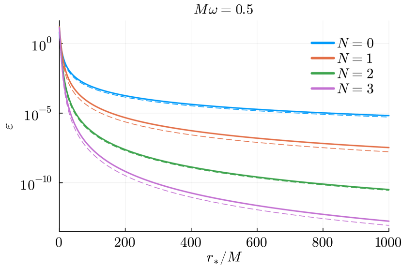
(a) for ansatz near infinity, $f^{\infty}_{\pm}$

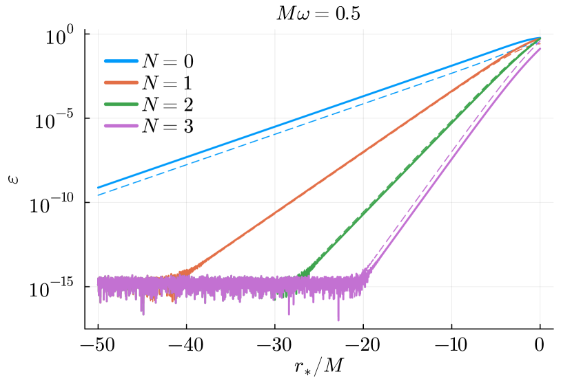
(b) for ansatz near the horizon, $g^{\mathrm{H}}_{\pm}$

Figure 8: Residual $\varepsilon$ of the ansatz (c.f. Eq. (52)) $f^{\infty}_{\pm}$ (upper panel) and $g^{\mathrm{H}}_{\pm}$ (lower panel) that we use in evaluating the initial conditions when solving for $X^{\mathrm{in,up}}$ and extracting the incidence and reflection amplitudes from the numerical solutions. In particular, we set $s=-2,\ell=2,m=2,a/M=0.7$ for the purpose of demonstration. For both plots, solid lines correspond to the out-going ansatzes and dash lines correspond to the in-going ansatzes truncated to different orders $N=0,1,2,3$ respectively.

Fig. 9 shows the residual $\varepsilon$ for the numerical GSN UP solutions in Fig. 7 (with $s=-2,\ell=2,m=2$, and $a/M=0.7$), for both $M\omega=0.5$ and $M\omega=1$. We see that the residuals are indeed very small, and stay roughly at $\varepsilon\approx 10^{-12}$, which is the absolute and relative tolerance given to the ODE solver. As for the numerical GSN IN solutions, the residuals are similar to that for the UP solutions.

The scaled Wronskian $\mathcal{W}_{X}$ (c.f. Eq. (39)) can be used as a sanity check. Using again the numerical solutions in Fig. 7 for the UP solution and Fig. 4 for the IN solution with $M\omega=0.5$ and $M\omega=1$, we evaluate the magnitude of the complex scaled Wronskian $|\mathcal{W}_{X}|$, which should be constant, at four different values of $r_{*}/M=-50,0,50,1000$ respectively. The scaled Wronskian can also be computed using the asymptotic amplitudes at infinity (c.f. Eq. (40)) and at the horizon (c.f. Eq. (41)) respectively. The values are tabulated in Tab. 1. We see that the scaled Wronskians computed from the numerical solutions for the two values of $M\omega$ are indeed constant, at least up to the eleventh digit, across the integration domain $r_{*}\in[-50M,1000M]$. This means that our method for solving GSN functions are numerically stable. The agreement of the scaled Wronskian evaluated at different locations in the integration domain and that evaluated using the asymptotic amplitudes at both boundaries also implies that our procedure of extracting incidence and reflection amplitudes from numerical solutions works.

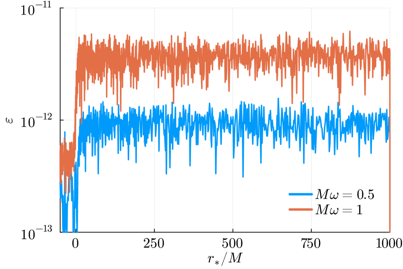
Figure 9: Residual $\varepsilon$ of the numerical GSN UP solutions shown in Fig. 7 for $M\omega=0.5$ and $M\omega=1$ respectively. Recall that both the absolute tolerance and the relative tolerance passed to the numerical ODE solver are set to $10^{-12}$.

$r_{*}/M$	$M\omega=0.5$	$M\omega=1$
$-\infty$	0.06686918718(132409)	0.09801150092(211632)
$-50$	0.06686918718(132406)	0.09801150092(220787)
$0$	0.06686918718(135844)	0.09801150092(220655)
$50$	0.06686918718(137257)	0.09801150092(220637)
$1000$	0.06686918718(173902)	0.09801150092(220587)
$\infty$	0.06686918718(244163)	0.09801150092(220785)

Table 1: Magnitude of the (complex) scaled Wronskian $|\mathcal{W}_{X}|$ of two frequencies, $M\omega=0.5$ and $M\omega=1$, evaluated at four different positions, $r_{*}/M=-50,0,50,1000$ respectively, and evaluated using the asymptotic amplitudes, with the GeneralizedSasakiNakamura.jl code. Digits beyond the eleventh digit are shown in brackets.

III.3.3 Comparisons with the Mano-Suzuki-Takasugi method

As mentioned in Sec. I, there are other ways of computing homogeneous solutions to the radial Teukolsky equation, and one of which is the MST method. Using the MST method, asymptotic amplitudes of Teukolsky functions (i.e. incidence and reflection amplitudes normalized by transmission amplitudes) can be determined accurately, together with the homogenous solutions themselves. Here we compare our numerical solutions and asymptotic amplitudes using the GSN formalism with that using the MST method. In particular, we use the implementation in the Teukolsky [46] Mathematica package from the Black Hole Perturbation Toolkit [36].

We compute the scaled Wronskian $\mathcal{W}_{R}$ of the numerical solutions for $s=-2,\ell=2,m=2,a/M=0.7$ mode for both $M\omega=0.5$ and $M\omega=1$ (the same setup as in Tab. 1), using the MST method. Similar to the case for GSN functions, we can compute $\mathcal{W}_{R}$ either from the numerical solutions $R^{\mathrm{in,up}}$ using Eq. (31), or from the asymptotic amplitudes using Eq. (32) or Eq. (33), and they should agree. In addition, the values for $\mathcal{W}_{R}$ should be the same as $\mathcal{W}_{X}$. The results are tabulated in Tab. 2. We see that the numbers shown in Tab. 1, which were computed using the GSN formalism, agree with the numbers in Tab. 2 at least up to the eleventh digit, testifying the numerical accuracy and correctness of the solutions and the asymptotic amplitudes computed using GeneralizedSasakiNakamura.jl. It should also be remarked that the implementation of the MST method in the Teukolsky package seems to be struggling either very close (e.g. $r_{*}=-50M$) or very far away (e.g. $r_{*}=1000M$) from the BH, and in general the MST method struggles more as $M\omega$ becomes larger while the GSN formalism becomes more efficient instead.

$r_{*}/M$	$M\omega=0.5$	$M\omega=1$
$-\infty$	0.06686918718(210336)	0.09801150092(219980)
$-50$	Aborted	Aborted
$0$	0.06686918718(210336)	0.09801150092(219978)
$50$	0.06686918718(210336)	Error
$1000$	Error	Error
$\infty$	0.06686918718(210336)	0.09801150092(219980)

Table 2: Magnitude of the (complex) scaled Wronskian $|\mathcal{W}_{R}|$ of two frequencies, $M\omega=0.5$ and $M\omega=1$, evaluated at four different positions, $r_{*}/M=-50,0,50,1000$ respectively, and evaluated using the asymptotic amplitudes, with the MST method implemented in the Teukolsky code. Note that in the computations we use the arbitrary-precision arithmetic in Mathematica (specifically 64-digit accurate). Digits beyond the eleventh digit are shown in brackets and truncated to the seventeenth digit to match Tab. 1. The computations at $r_{*}=-50M$ for both cases were aborted after running for an hour.

IV Conclusion and future work

In this paper, we have revamped the Generalized Sasaki-Nakamura (GSN)formalism for computing homogeneous solutions to both the GSN equation and the radial Teukolsky equation for scalar, electromagnetic and gravitational perturbations. Specifically, we have provided explicitly expressions for the transformations between the Teukolsky formalism and the GSN formalism. We have also derived expressions for higher-order corrections to asymptotic solutions of the GSN equation, as well as frequency-dependent conversion factors between asymptotic solutions in the Teukolsky and the GSN formalism. Both are essential for using the GSN formalism to perform numerical work. We have also described an open-source implementation of the now-complete GSN formalism for solving homogeneous solutions, where the implementation re-formulated the GSN equation further into a Riccati equation so as to gain extra efficiency at high frequencies.

In the following we discuss two potential applications of the GSN formalism in BH perturbation theory, namely as an efficient procedure for computing gravitational radiation from BHs, and as an alternative method for QNM determination.

IV.1 An efficient procedure for computing gravitational radiation from Kerr black holes

As we have demonstrated in Sec. III.3, the GSN formalism is capable of producing accurate and stable numerical solutions to the homogenous GSN equation, which can then be converted to numerical Teukolsky functions, across a wide range of $r_{*}/M$ when the MST method tends to struggle when $r_{*}/M\ll 1$ and $r_{*}/M\gg 1$ as shown in Sec. III.3.3. While we have only shown the numerical results for $M\omega=0.5$ and $M\omega=1$ explicitly, it is reasonable to expect the formalism to also work for other frequencies, if not even better at high frequencies when we gain extra efficiency by further transforming a GSN function $X(r_{*})$ into a complex frequency function $d\Phi/dr_{*}$, while the MST method requires a much higher working precision for computation. This can occur, for example, when computing a higher harmonic of an extreme mass-ratio inspiral (EMRI) waveform. For a generic orbit, the harmonic has a frequency $\omega$ given by [48]

$$\omega=m\Omega_{\phi}+k\Omega_{\theta}+n\Omega_{r},$$ (70)

where $\Omega_{\phi},\Omega_{\theta},\Omega_{r}$ are the fundamental orbital frequency for the $\phi$-, $\theta$- and $r$- motion respectively.

Indeed, we see from Sec. III.3.1 that in some regions of the parameter space, it is more efficient to solve for the complex frequency function $d\Phi/dr_{*}$ than to solve for the GSN function $X$ itself. There are, however, cases where the reverse is true instead, especially at a lower wave frequency when the BH potential barrier is less transmissive, since it is numerically more efficient (requiring fewer nodes) to track a less oscillatory function than a more oscillatory function (c.f. Fig. 4). This means that a better numerical scheme solving for $X^{\mathrm{in,up}}$ (and by extension $R^{\mathrm{in,up}}$) can be formulated by first solving the first-order non-linear ODE for $d\Phi/dr_{*}$, and then “intelligently” switching to solving the second-order linear ODE for $X$ when it is more efficient, for example, when $d/dr_{*}(d\hat{\Phi}/dr_{*})$ is above some pre-defined threshold. This hybrid approach is similar in sprit to some of the state-of-the-art solvers for oscillatory second order linear ODEs [49].

While the GSN formalism is a great alternative to the MST method for computing homogeneous solutions (i.e. $T=0$) to the radial Teukolsky equation, the real strength of the GSN formalism is the ability to also compute inhomogeneous solutions (i.e. $T\neq 0$). Given an extended Teukolsky source term, such as a plunging test particle from infinity, the convolution integral with the Teukolsky functions can be divergent when using the Green’s function method to compute the inhomogeneous solution and regularization of the integral is needed [50, 51]. In Ref. [33], Sasaki and Nakamura had worked out a formalism, which was developed upon their SN transformation, to compute the inhomogeneous solution for $s=-2$ where the new source term, constructed from the Teukolsky source term, is short-ranged such that the convolution integral with the SN functions is convergent when using the Green’s function method.

In a forthcoming paper, we show that their construction can also be extended to work for $s=2$, and the corresponding GSN transformation, in a similar fashion, serves as the foundation of the method. This will be important for studying near-horizon physics [52, 53, 54], such as computing gravitational radiation from a point particle plunging towards a BH as observed near the horizon, where the polarization contents are encoded in $\psi_{0}$ (with $s=2$) instead of $\psi_{4}$ (with $s=-2$). In particular, the Teukolsky-Starobinsky identities [55, 23] are not valid in this case (since the source term does not vanish near the horizon) and we cannot use them to convert the asymptotic amplitude for $\psi_{4}$ to that for $\psi_{0}$.

IV.2 An alternative method for quasi-normal mode determination

The re-formulation of a Schrödinger-like equation into a Riccati equation introduced in Sec. III.1.1 is not new and had actually been used previously, for instance, in the seminal work by Chandrasekhar and Detweiler on QNMs of Schwarzschild BHs [57]. It was used (c.f. Eq. (5) of Ref. [57]) to alleviate the numerical instability associated with directly integrating the Zerilli equation, and equivalently also the Regge-Wheeler equation to which the GSN equation reduces in the non-spinning limit. Therefore, it is reasonable to expect that the re-formulation to be useful for determining QNM frequencies and their associated radial solutions.

Recall that a QNM solution is both purely-ingoing at the horizon and purely-outgoing at infinity. In terms of the asymptotic amplitudes of the corresponding Teukolsky function (c.f. Eq. (29) and Eq. (30)) at a particular frequency $\omega_{\mathrm{QNM}}$, we have

$$B^{\mathrm{inc}}_{\mathrm{T}}(\omega_{\mathrm{QNM}})=C^{\mathrm{inc}}_{\mathrm{T}}(\omega_{\mathrm{QNM}})=0$$ (71)

$$\Rightarrow\mathcal{W}_{R}(\omega_{\mathrm{QNM}})=0,$$

where the second line uses Eq. (32). This means that searching for QNM frequencies is the same as searching for zeros of $\mathcal{W}_{R}$, the scaled Wronskian for Teukolsky functions. Also recall that in App. C, we proved that the scaled Wronskian for Teukolsky functions $\mathcal{W}_{R}$ and that for the corresponding GSN functions $\mathcal{W}_{X}$ are the same, implying that the QNM spectra for Teukolsky functions coincide with the QNM spectra for GSN functions. Thus, we can use the GSN equation, which has a short-ranged potential, instead of the Teukolsky equation for determining the QNM frequencies and the corresponding excitation factors (after applying the conversion factors shown in App. E).

Indeed, Glampedakis and Andersson proposed methods to calculate QNM frequencies and excitation factors given a short-ranged potential [58], alternative to the Leaver’s method [59]. They demonstrated their methods by computing a few of the QNM frequencies for scalar perturbations ($s=0$) and gravitational perturbations ($|s|=2$), as well as the QNM excitation factors for scalar perturbations of Kerr BHs. Together with the GSN transformations and the asymptotic solutions from this paper, it is straightforward to compute the QNM frequencies and their excitation factors for scalar, electromagnetic, and gravitational perturbations using the GSN formalism. We leave this for future work.

Appendix A Angular Teukolsky equation

After performing the separation of variables to the Teukolsky equation in Eq. (2) using an ansatz of the form $\psi(t,r,\theta,\phi)=R(r)S(\theta,\phi)e^{-i\omega t}$, the equation is separated into two parts: the angular part and the radial part. In this appendix, we focus only on solving the angular part (aptly named the angular Teukolsky equation) numerically, and the radial part is treated in the main text.

Let us define ${}_{s}S_{\ell m\omega}(\theta,\phi)\equiv{}_{s}S_{\ell m}(x\equiv\cos\theta;c\equiv a\omega)e^{im\phi}$, where the integer $m$ labels the (trivial) eigenfunctions that satisfy the azimuthal symmetry. The angular Teukolsky equation then reads

$$\dfrac{d}{dx}\left[(1-x^{2})\dfrac{d}{dx}{}_{s}S_{\ell m}(x;c)\right]+\\ \left[(cx)^{2}-2csx+s+{}_{s}\mathcal{A}_{\ell m}(c)-\frac{(m+sx)^{2}}{1-x^{2}}\right]{}_{s}S_{\ell m}(x;c)=0,$$ (72)

where ${}_{s}\mathcal{A}_{\ell m}$ is the angular separation constant and it is related to $\lambda$ (c.f. Eq. (4)) by

$$\lambda={}_{s}\mathcal{A}_{\ell m}+c^{2}-2mc.$$ (73)

The angular Teukolsky equation is solved under the boundary conditions that the solutions at $x=\pm 1$ (or equivalently at $\theta=0,\pi$) are finite, and the solutions are also known as the spin-weighted spheroidal harmonics, denoted by ${}_{s}S_{\ell m\omega}(\theta,\phi)$.

There are multiple methods for solving the angular Teukolsky equation numerically, such as Leaver’s continued fraction method [59]. A spectral decomposition method for solving the angular Teukolsky equation can be formulated [63, 64] by writing a spin-weighted spheroidal harmonic ${}_{s}S_{\ell m\omega}(\theta,\phi)$ as a sum of spin-weighted spherical harmonics ${}_{s}Y_{\ell m}(\theta,\phi)$. The details for such a formulation can be found in, for example, Ref. [63] and Ref. [64]. We briefly summarize the method here, mostly following and using the notations in Ref. [64], for the sake of completeness.

A.1 Spectral decomposition method

A spin-weighted spheroidal harmonic ${}_{s}S_{\ell m}(x;c)$ is expanded using spin-weighted spherical harmonics ${}_{s}Y_{\ell m}(\theta)$, or equivalently ${}_{s}S_{\ell m}(x;0)$ as [64]

$${}_{s}S_{\ell m}(x;c) =\sum_{\ell^{\prime}=\ell_{\mathrm{min}}}^{\infty}{}_{s}C_{\ell^{\prime}\ell m}(c)\;{}_{s}S_{\ell^{\prime}m}(x;0)$$ (74)

$$=\left(\vec{C}_{\ell}\right)^{T}\vec{S}_{\ell},$$

where $\ell_{\mathrm{min}}=\max(|m|,|s|)$ and ${}_{s}C_{\ell^{\prime}\ell m}(c)$ is the expansion coefficient of the $\ell$-th spheroidal harmonic with the $\ell^{\prime}$-th spherical harmonic (of the same value of $s$ and $m$ and we drop them in the subscripts hereafter), as a function of $c\equiv a\omega$. Equivalently, we can define two column vectors $\vec{C}_{\ell}$ and $\vec{S}_{\ell}$, where the rows are labelled by the index $\ell^{\prime}$. For example, the first row of the vectors (of index $\ell^{\prime}=\ell_{\mathrm{min}}$) are ${}_{s}C_{\ell_{\mathrm{min}}\ell m}$ and ${}_{s}S_{\ell_{\mathrm{min}}m}(x;0)$ respectively. The index for the rows goes up to $\ell^{\prime}=\ell_{\mathrm{max}}\to\infty$, and the vectors have a size of $\ell_{\mathrm{max}}-\ell_{\mathrm{min}}+1$. Then the spin-weighted spheroidal harmonic $S_{\ell}(x;c)$ is the dot product of the two vectors.

Substituting Eq. (74) into Eq. (72), we get an eigenvalue equation [64]

$$\mathbb{M}\vec{C}_{\ell}=\mathcal{A}_{\ell}\vec{C}_{\ell},$$ (75)

where $\mathbb{M}$ is a $\left(\ell_{\mathrm{max}}-\ell_{\mathrm{min}}+1\right)\times\left(\ell_{\mathrm{max}}-\ell_{\mathrm{min}}+1\right)$ matrix, and recall that $\mathcal{A}_{\ell}\equiv{}_{s}\mathcal{A}_{\ell m}(c\equiv a\omega)$ is the angular separation constant (after writing back all the subscripts). The matrix elements $\mathbb{M}_{\ell\ell^{\prime}}$ are given by [64]

$$\mathbb{M}_{\ell\ell^{\prime}}=\begin{cases}-c^{2}\mathbb{A}_{\ell^{\prime}m}&\mathrm{if}\;\;\ell^{\prime}=\ell-2,\\ -c^{2}\mathbb{D}_{\ell^{\prime}m}+2cs\mathbb{F}_{\ell^{\prime}m}&\mathrm{if}\;\;\ell^{\prime}=\ell-1,\\ \mathcal{A}_{\ell^{\prime}}(0)-c^{2}\mathbb{B}_{\ell^{\prime}m}+2cs\mathbb{H}_{\ell^{\prime}m}&\mathrm{if}\;\;\ell^{\prime}=\ell,\\ -c^{2}\mathbb{E}_{\ell^{\prime}m}+2cs\mathbb{G}_{\ell^{\prime}m}&\mathrm{if}\;\;\ell^{\prime}=\ell+1,\\ -c^{2}\mathbb{C}_{\ell^{\prime}m}&\mathrm{if}\;\;\ell^{\prime}=\ell+2,\\ 0&\mathrm{otherwise.}\\ \end{cases},$$ (76)

where

$$\mathbb{A}_{\ell m} = \mathbb{F}_{\ell m}\mathbb{F}_{(\ell+1)m},$$ (77a)

$$\mathbb{B}_{\ell m} = \mathbb{F}_{\ell m}\mathbb{G}_{(\ell+1)m}+\mathbb{G}_{\ell m}\mathbb{F}_{(\ell-1)m}+\mathbb{H}_{\ell m}^{2},$$ (77b)

$$\mathbb{C}_{\ell m} = \mathbb{G}_{\ell m}\mathbb{G}_{(\ell-1)m},$$ (77c)

$$\mathbb{D}_{\ell m} = \mathbb{F}_{\ell m}\mathbb{H}_{(\ell+1)m}+\mathbb{F}_{\ell m}\mathbb{H}_{\ell m},$$ (77d)

$$\mathbb{E}_{\ell m} = \mathbb{G}_{\ell m}\mathbb{H}_{(\ell-1)m}+\mathbb{G}_{\ell m}\mathbb{H}_{\ell m},$$ (77e)

$$\mathbb{F}_{\ell m} = \sqrt{\dfrac{(\ell+1)^{2}-m^{2}}{(2\ell+3)(2\ell+1)}\dfrac{(\ell+1)^{2}-s^{2}}{(\ell+1)^{2}}},$$ (77f)

$$\mathbb{G}_{\ell m} = \begin{cases}\sqrt{\dfrac{\ell^{2}-m^{2}}{4\ell^{2}-1}\dfrac{\ell^{2}-s^{2}}{\ell^{2}}}&\mathrm{if}\;\;\ell\neq 0\\ 0&\mathrm{if}\;\;\ell=0\end{cases},$$ (77g)

$$\mathbb{H}_{\ell m} = \begin{cases}-\dfrac{ms}{\ell(\ell+1)}&\mathrm{if}\;\;\ell\neq 0\;\;\mathrm{and}\;\;s\neq 0\\ 0&\mathrm{if}\;\;\ell=0\;\;\mathrm{or}\;\;s=0\end{cases},$$ (77h)

$$\mathcal{A}_{\ell}(0) = \ell(\ell+1)-s(s+1).$$ (77i)

Solving the angular Teukolsky equation now amounts to solving the eigenvalue problem in Eq. (75) for the eigenvalue $\mathcal{A}_{\ell}$ and the eigenvector $\vec{C}_{\ell}$. The spin-weighted spheroidal harmonic can then be constructed using the eigenvector $\vec{C}_{\ell}$ and the corresponding spin-weight spherical harmonics with Eq. (74). In practice, we cannot solve a matrix eigenvalue problem of infinite size and we truncate the column vector $\vec{C}_{\ell}$ to have a finite value of $\ell_{\mathrm{max}}$. The accuracy of the numerical eigenvalue and eigenvector solution depends on the size of the truncated matrix.

SpinWeightedSpheroidalHarmonics.jl is our open-source implementation of the abovementioned spectral decomposition method for solving spin-weighted spheroidal harmonics in julia. The code solves the truncated version of Eq. (75) to obtain the angular separation constant ${}_{s}\mathcal{A}_{\ell m}$ and the eigenvector ${}_{s}\vec{C}_{\ell m}$. Apart from the angular separation constant, the code can also compute the separation constant $\lambda$ (c.f. Eq. (4)), and evaluate numerical values of spin-weight spheroidal harmonics and their derivatives. In particular, the code adopts the normalization convention for ${}_{s}S_{\ell m\omega}(\theta,\phi)$ that

$$\int_{0}^{\pi}\left[{}_{s}S_{\ell m}(\theta;c)\right]^{2}\sin(\theta)\,d\theta=\frac{1}{2\pi}.$$ (78)

To evaluate numerical values of the spin-weighted spheroidal harmonics ${}_{s}S_{\ell m\omega}(\theta,\phi)$ and their derivatives, it is necessary to also be able to numerically (and possibly efficiently) evaluate the spin-weighted spheroidal harmonics ${}_{s}Y_{\ell m}(\theta,\phi)$.

A.2 Evaluation of ${}_{s}S_{\ell m\omega}(\theta,\phi)$

Recall from Eq. (74) that the spin-weighted spheroidal harmonic ${}_{s}S_{\ell m\omega}(\theta,\phi)$ is expanded in terms of the spin-weighted spherical harmonics, i.e.

$${}_{s}S_{\ell m}(\theta,\phi;a\omega)=\sum_{\ell^{\prime}=\ell_{\mathrm{min}}}^{\infty}{}_{s}C_{\ell^{\prime}\ell m}(a\omega)\;{}_{s}Y_{\ell m}(\theta,\phi),$$

and the spectral decomposition method solves for the expansion coefficients ${}_{s}C_{\ell^{\prime}\ell m}(a\omega)$, which is only part of the ingredients. It is possible to evaluate ${}_{s}Y_{\ell m}(\theta,\phi)$ exactly, and the expression is given by [65]

$$\begin{aligned} {}_{s}Y_{\ell m}(\theta,\phi)&=(-1)^{m}e^{im\phi}\sqrt{\frac{(\ell+m)!(\ell-m)!(2\ell+1)}{4\pi(\ell+s)!(\ell-s)!}}\\ &\times\sum_{r=0}^{\ell-s}\left[\binom{\ell-s}{r}\binom{\ell+s}{r+s-m}(-1)^{\ell-r-s}\right.\\ &\times\left.\cos^{2r+s-m}(\frac{\theta}{2})\sin^{2\ell-2r-s+m}(\frac{\theta}{2})\vphantom{}\right]\end{aligned}.$$ (79)

In principle, obtaining the value of a spin-weighted spherical harmonic ${}_{s}Y_{\ell m}(\theta,\phi)$ is as simple as evaluating the sum as shown in Eq. (79). Oftentimes, however, when we solve the eigenvalue problem in Eq. (75), the index $\ell$ can be big enough so that a direct evaluation of the pre-factor

$$\sqrt{\frac{(\ell+m)!(\ell-m)!}{(\ell+s)!(\ell-s)!}}$$

in Eq. (79) on a machine can cause an overflow error because of the large factorials involved in the computation. Fortunately, the expression for the pre-factor can be simplified. In fact,

$$\sqrt{\dfrac{(\ell+m)!(\ell-m)!}{(\ell+s)!(\ell-s)!}}=\begin{cases}\sqrt{\dfrac{\left(\ell-m\right)\left(\ell-m-1\right)\dots\left(\ell-m-(s-m)+1\right)}{\left(\ell+m+(s-m)\right)\left(\ell+m+(s-m)-1\right)\dots\left(\ell+m+1\right)}}&\mathrm{if}\;\;s>m,\\ \sqrt{\dfrac{\left(\ell+s+(m-s)\right)\left(\ell+s+(m-s)-1\right)\dots\left(\ell+s+1\right)}{\left(\ell-s\right)\left(\ell-s-1\right)\dots\left(\ell-s-(m-s)+1\right)}}&\mathrm{if}\;\;s<m,\\ 1&\mathrm{if}\;\;|s|=|m|.\end{cases},$$ (80)

and now evaluations of ${}_{s}S_{\ell m\omega}(\theta,\phi)$ using Eq. (74) are free from overflow.

A.3 Evaluation of $\partial_{\theta,\phi}^{n}\;{}_{s}S_{\ell m\omega}(\theta,\phi)$

In order to evaluate partial derivatives of spin-weighted spheroidal harmonics, $\partial_{\theta,\phi}^{n}\;{}_{s}S_{\ell m\omega}(\theta,\phi)$, which are needed for evaluating source terms $T$ of the Teukolsky equation (c.f. Eq. (2)), we can use the fact that the expansion coefficients ${}_{s}C_{\ell^{\prime}\ell m}(c\equiv a\omega)$ in Eq. (74) are independent of $\theta$ and $\phi$. This means that the partial derivatives $\partial_{\theta,\phi}^{n}\;{}_{s}S_{\ell m\omega}(\theta,\phi)$ are given by the sum of the partial derivatives of ${}_{s}Y_{\ell m}(\theta,\phi)$ with the same set of the expansion coefficients, i.e.

$$\left(\dfrac{\partial}{\partial\left\{\theta,\phi\right\}}\right)^{n}\;{}_{s}S_{\ell m\omega}(\theta,\phi)=\\ \sum_{\ell^{\prime}=\ell_{\mathrm{min}}}^{\infty}\left[{}_{s}C_{\ell^{\prime}\ell m}(a\omega)\;\left(\dfrac{\partial}{\partial\left\{\theta,\phi\right\}}\right)^{n}{}_{s}Y_{\ell m}(\theta,\phi)\right].$$ (81)

In principle, we can evaluate the partial derivatives using AD. However, the evaluation can be more performant by noticing that the exact evaluation of the partial derivative with respect to $\phi$ is trivial because of the $e^{im\phi}$ dependence. Each partial differentiation with respect to $\phi$ gives a factor of $im$. As for the partial derivative of a spin-weighted spherical harmonic with respect to $\theta$, the computation scheme is less trivial. Note that each term in Eq. (79) is of the form $c_{r}\cos^{\alpha_{r}}(\theta/2)\sin^{\beta_{r}}(\theta/2)$, where $r$ is the summation index and $c_{r}$ is the pre-factor with $\alpha_{r}$ and $\beta_{r}$ being the exponent for the $\cos(\theta/2)$ and $\sin(\theta/2)$ factor respectively. Each partial differentiation with respect to $\theta$ splits the term into two terms, one with $(c_{r}/2)\beta_{r}\cos^{\alpha_{r}+1}(\theta/2)\sin^{\beta_{r}-1}(\theta/2)$, and one with $(-c_{r}/2)\alpha_{r}\cos^{\alpha_{r}-1}(\theta/2)\sin^{\beta_{r}+1}(\theta/2)$.

We can keep track of the coefficients and the exponents for the cosine and the sine factor with the help of a binary tree. We represent each term in the summation with index $r$ in Eq. (79) as the root node of a tree (for an illustration, see Fig. 10) with an entry of three numbers $\left(c_{r},\alpha_{r},\beta_{r}\right)$. Each partial differentiation with respect to $\theta$ corresponds to adding two child nodes with the entry $\left(c_{r}\beta_{r}/2,\alpha_{r}+1,\beta_{r}-1\right)$ and $\left(-c_{r}\alpha_{r}/2,\alpha_{r}-1,\beta_{r}+1\right)$ respectively. Therefore, the $n$-th order partial derivative of $\theta$ can be evaluated exactly by traversing all the nodes of depth $n$ and then summing over their contributions.

Figure 10: Binary tree representation of a term and its partial derivatives with respect to $\theta$ in the summation of Eq. (79). In each node, the three numbers correspond to the pre-factor, the exponent for the $\cos(\theta/2)$ and the $\sin(\theta/2)$ factor respectively. A partial differentiation with respect to $\theta$ creates two leaf nodes with the pre-factor and the exponents computed according to rules of partial differentiation. The $n$-th partial derivative with respect to $\theta$ of the term in the root node can be evaluated by simply summing over all the nodes of depth $n$.

Appendix B Fast inversion from the tortoise coordinate $r_{*}$ to the Boyer-Lindquist coordinate $r$

The tortoise coordinate $r_{*}$ (for Kerr BHs) is defined by

$$\dfrac{dr_{*}}{dr}=\dfrac{r^{2}+a^{2}}{\Delta}=\dfrac{r^{2}+a^{2}}{\left(r-r_{+}\right)\left(r-r_{-}\right)}.$$ (82)

Using Eq. (7) one can generate different “tortoise coordinate” which differ to each other only by an integration constant. Here, and in most of the literature, we choose the integration constant such that

$$r_{*}(r)=r+\frac{2r_{+}}{r_{+}-r_{-}}\ln\left(\frac{r-r_{+}}{2}\right)-\frac{2r_{-}}{r_{+}-r_{-}}\ln\left(\frac{r-r_{-}}{2}\right).$$ (82)

However, there is no simple analytical expression that gives $r=r(r_{*})$, and one will have to instead numerically invert Eq. (14). Such an inversion scheme that is both fast and accurate is needed for our numerical implementation of the GSN formalism because we numerically solve the GSN equation in the $r_{*}$-coordinate instead of the Boyer-Lindquist $r$-coordinate, and yet the GSN potentials, which will be evaluated at many different values of $r_{*}$ during the numerical integration, are written in terms of $r$.

This coordinate inversion is equivalent to a root-finding problem. Given a value of the tortoise coordinate $r_{*}^{0}$, we solve for $h^{0}\equiv\left(r^{0}-r_{+}\right)>0$ that satisfies

$$r_{*}^{0}-r_{*}(r_{+}+h^{0})=0,$$ (83)

in order to find the corresponding Boyer-Lindquist coordinate $r^{0}\equiv r_{+}+h^{0}$ that is outside the horizon .

Fig. 11 shows a plot of $r$ as a function of $r_{*}$ for $a/M=0.7$. As the value of $r_{*}$ becomes larger, the simple approximation $r(r_{*})\approx r_{*}$ works better. In fact, the slope $dr/dr_{*}\to 1$ as $r_{*}\gg 0$. Therefore, derivative-based methods such as the Newton-Raphson method and secant methods [34] are efficient in performing the coordinate inversion (since we can evaluate the derivatives exactly and cheaply). However, these methods are going to be inefficient for negative values of $r_{*}$ near the horizon since the slope tends to zero.

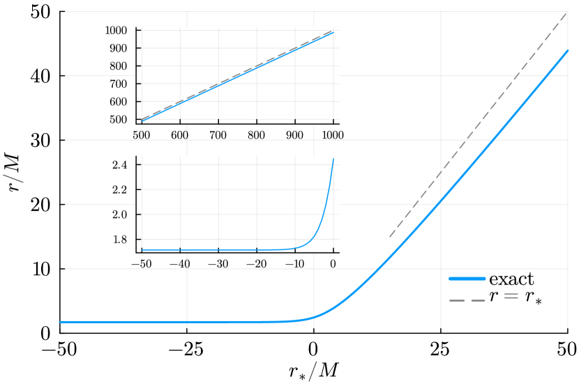
Figure 11: The Boyer-Lindquist $r$-coordinate as a function of the tortoise $r_{*}$ coordinate for $a/M=0.7$. As the value of $r_{*}$ becomes larger (upper inset), the approximation $r(r_{*})\approx r_{*}$ (dashed) gets increasingly better as $dr/dr_{*}\to 1$. Meanwhile as the value of $r_{*}$ becomes more negative (lower inset), $r(r_{*})$ approaches $r=r_{+}$ as constructed and $dr/dr_{*}\to 0$.

In our numerical implementation, we use a hybrid of root-finding algorithms. For $r_{*}^{0}>0$, we use the Newton-Raphson method [34] with an initial guess of $h=r_{*}^{0}$, and switch to using the bisection method [34] for $r_{*}^{0}\leq 0$. To use the bisection method, an interval of $h$ that contains the root of Eq. (83) is given to the algorithm as an initial guess. Since $r=r_{+}$ maps to $r_{*}\to-\infty$, a natural choice for the lower bound of the bracketing interval would be $h=0$. For the upper bracketing bound, from Fig. 12 we see that the value of $h$ that corresponds to $r_{*}=0$ is a monotonically-increasing function of the spin magnitude $|a|$. Therefore, we can simply choose the upper bound value to be (equal to or greater than) the limiting value of $h$ that corresponds to $r_{*}=0$ when $|a|\to 1$. Explicitly, the numerical implementation in GeneralizedSasakiNakamura.jl uses the bracketing interval $0<h<1.4$.

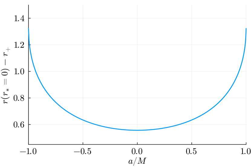
Figure 12: The difference between $r_{*}=0$ and the horizon in the Boyer-Lindquist $r$-coordinate, $r(r_{*}=0)-r_{+}$, as a function of the spin $a$ of the BH. We see that the difference is monotonically increasing with $|a|$, and it is the smallest when $a=0$, and the largest ($\approx 1.3$) when $|a|\to 1$. We can use this to construct an interval of $r$ that must contain $r=r(r_{*})$ for $r_{*}\leq 0$ when using the bisection method.

Appendix C Deriving the identity between the scaled Wronskians for Teukolsky functions and Generalized Sasaki-Nakamura functions

Recall that the scaled Wronskian $\mathcal{W}_{R}$ for the Teukolsky functions $R^{\mathrm{in,up}}$ is defined by

$$\mathcal{W}_{R}=\Delta^{s+1}\left(R^{\mathrm{in}}{R^{\mathrm{up}}}^{\prime}-R^{\mathrm{up}}{R^{\mathrm{in}}}^{\prime}\right),$$ (84)

whereas the scaled Wronskian $\mathcal{W}_{X}$ for the GSN functions $X^{\mathrm{in,up}}$ is defined by

$$\mathcal{W}_{X}=\dfrac{1}{\eta}\left[X^{\mathrm{in}}(dX^{\mathrm{up}}/dr_{*})-(dX^{\mathrm{in}}/dr_{*})X^{\mathrm{up}}\right].$$ (85)

They are called scaled Wronskians because they are not the same as “ordinary” Wronskians. For a generic second-order linear ODE

$$\dfrac{d^{2}y(x)}{dx^{2}}+p(x)\dfrac{dy(x)}{dx}+q(x)y(x)=0,$$ (86)

suppose it admits two linearly-independent solutions $y_{1}(x)$ and $y_{2}(x)$, then the Wronskian $W(x)$ is defined by

$$W(x)=y_{1}\dfrac{dy_{2}}{dx}-y_{2}\dfrac{dy_{1}}{dx},$$ (87)

which is a function of $x$ in general. It can be shown that $W(x)$ satisfies the ODE [66]

$$\dfrac{dW}{dx}+p(x)W=0.$$ (88)

Let us define the scaled Wronskian $\mathcal{W}$ such that

$$\mathcal{W}\equiv\exp\left(\int^{x}p(x^{\prime})\;dx^{\prime}\right)W(x),$$ (89)

we see that $d\mathcal{W}/dx=0$, i.e. $\mathcal{W}$ is a constant.

It is not immediately obvious that $\mathcal{W}_{X}$, evaluated using Eq. (39), is the same as $\mathcal{W}_{R}$, evaluated using Eq. (31). From Eq. (39) and using Eq. (7), we have

$$\mathcal{W}_{X}=\dfrac{\Delta}{(r^{2}+a^{2})\eta}\left(X^{\mathrm{in}}{X^{\mathrm{up}}}^{\prime}-X^{\mathrm{up}}{X^{\mathrm{in}}}^{\prime}\right).$$ (90)

Recall that the GSN function $X$ is transformed from a Teukolsky function $R$ using the ${}_{s}\Lambda$ operator that

$$X(r) ={}_{s}\Lambda\left[R(r)\right]$$ (91)

$$=\sqrt{\left(r^{2}+a^{2}\right)\Delta^{s}}\left[\left(\alpha+\beta\Delta^{s+1}\dfrac{d}{dr}\right)R(r)\right].$$

One can show that

$$X^{\mathrm{in}}{X^{\mathrm{up}}}^{\prime}-X^{\mathrm{up}}{X^{\mathrm{in}}}^{\prime}$$ (92)

$$= \left(r^{2}+a^{2}\right)\Delta^{s}\left\{\eta-(s+1)\alpha\beta\Delta^{s}\left[2\left(r-1\right)-\Delta^{\prime}\right]\right\}$$

$$\times\left(R^{\mathrm{in}}{R^{\mathrm{up}}}^{\prime}-R^{\mathrm{up}}{R^{\mathrm{in}}}^{\prime}\right)$$

$$= \dfrac{\left(r^{2}+a^{2}\right)\eta}{\Delta}\Delta^{s+1}\left(R^{\mathrm{in}}{R^{\mathrm{up}}}^{\prime}-R^{\mathrm{up}}{R^{\mathrm{in}}}^{\prime}\right)$$

$$= \dfrac{\left(r^{2}+a^{2}\right)\eta}{\Delta}\mathcal{W}_{R},$$

using Eq. (10) and the fact that $\Delta^{\prime}=2(r-1)$. From here, we see that indeed

$$\mathcal{W}_{X}=\mathcal{W}_{R}.$$ (93)

Appendix D Recurrence relations for the higher order corrections to the asymptotic boundary conditions of the Generalized Sasaki-Nakamura equation

In addition to the asymptotic boundary conditions to the leading order as shown in Eq. (37) and (38), it is useful to also compute these boundary conditions to higher orders. To start off, we assume the following ansatz for the GSN function

$$X(r_{*})\sim\begin{cases}f^{\infty}_{\pm}(r)e^{\pm i\omega r_{*}},&r_{*}\to\infty\\ g^{\mathrm{H}}_{\pm}(r)e^{\pm ipr_{*}},&r_{*}\to-\infty\end{cases}.$$ (94)

By substituting the ansatz in Eq. (52) into the GSN equation in Eq. (22), it can be shown that as $r\to\infty$, the functions $f^{\infty}_{\pm}$ satisfy the following second-order ODE

$${f^{\infty}_{\pm}}^{\prime\prime}+P^{\infty}_{\pm}(r){f^{\infty}_{\pm}}^{\prime}+Q_{\pm}^{\infty}(r){f^{\infty}_{\pm}}=0,$$ (95)

where we define the functions

$$P_{\pm}^{\infty}(r) =\left(\dfrac{r^{2}+a^{2}}{\Delta}\right)\left[\left(\dfrac{\Delta}{r^{2}+a^{2}}\right)^{\prime}\pm 2i\omega-\mathcal{F}\right],$$ (96)

$$Q_{\pm}^{\infty}(r) =\left(\dfrac{r^{2}+a^{2}}{\Delta}\right)^{2}\left(-\omega^{2}\mp i\omega\mathcal{F}-\mathcal{U}\right).$$ (97)

As $r\to r_{+}$, the functions $g^{\mathrm{H}}_{\pm}$ satisfy the following second-order ODE

$${g^{\mathrm{H}}_{\pm}}^{\prime\prime}+P^{\mathrm{H}}_{\pm}(r){g^{\mathrm{H}}_{\pm}}^{\prime}+Q_{\pm}^{\mathrm{H}}(r){g^{\mathrm{H}}_{\pm}}=0,$$ (98)

where we define the functions

$$P_{\pm}^{{\mathrm{H}}}(r) =\left(\dfrac{r^{2}+a^{2}}{\Delta}\right)\left[\left(\dfrac{\Delta}{r^{2}+a^{2}}\right)^{\prime}\pm 2ip-\mathcal{F}\right],$$ (99)

$$Q_{\pm}^{{\mathrm{H}}}(r) =\left(\dfrac{r^{2}+a^{2}}{\Delta}\right)^{2}\left(-p^{2}\mp ip\mathcal{F}-\mathcal{U}\right).$$ (100)

We look for formal series expansions of the solutions $f^{\infty}_{\pm}$ at infinity and $g^{\mathrm{H}}_{\pm}$ at the horizon respectively. We then truncate these expansions at an arbitrary order and use them to set the boundary conditions when solving the GSN equation on a numerically-finite interval.

D.1 Formal series expansion about infinity

Inspecting Eq. (95) with $P_{\pm}^{\infty}(r)$ and $Q_{\pm}^{\infty}(r)$ defined in Eq. (96) and (97) respectively and performing the standard change of variable $z\equiv 1/r$, we see that infinity (i.e. $z=0$) is an irregular singularity of rank $1$. We expand $P_{\pm}^{\infty}(r)$ and $Q_{\pm}^{\infty}(r)$ as $r\to\infty$ with

$$P_{\pm}^{\infty}(r) =\sum_{j=0}^{\infty}\dfrac{P_{\pm,j}^{\infty}}{r^{j}},$$ (101)

$$Q_{\pm}^{\infty}(r) =\sum_{j=0}^{\infty}\dfrac{Q_{\pm,j}^{\infty}}{r^{j}}.$$ (102)

In particular, we find that $Q_{\pm,0}^{\infty}$ and $Q_{\pm,1}^{\infty}$ are zero. Using these facts, the functions $f^{\infty}_{\pm}$ have the following formal series expansions near infinity as [67]

$$f^{\infty}_{\pm}(r)=e^{\nu_{\pm}r}r^{\kappa_{\pm}}\sum_{j=0}^{\infty}\dfrac{a_{\pm,j}}{r^{j}},$$ (103)

(note that we suppress the $\infty$ superscript on the RHS since the context is clear) where $\kappa_{\pm}$ is given by

$$\kappa_{\pm}=-\dfrac{P_{\pm,1}\nu_{\pm}+Q_{\pm,1}}{P_{\pm,0}+2\nu_{\pm}},$$ (104)

and $\nu_{\pm}$ is a solution to the characteristic equation

$$\nu_{\pm}^{2}-P_{\pm,0}\nu_{\pm}=0.$$ (105)

There are two solutions to the characteristic equation: $\nu_{\pm}=0$ or $\nu_{\pm}=P_{\pm,0}$. We pick $\nu_{+}=\nu_{-}=0$ as this gives the desired form for the series expansions and as a result we have both $\kappa_{+}=\kappa_{-}=0$ (recall that $Q_{\pm,1}=0$). The expansion coefficients $a_{\pm,j}$ can be evaluated using the recurrence relation [67]

$$P_{0}ja_{j}=j(j-1)a_{j-1}+\sum_{k=1}^{j}\left[Q_{k+1}-\left(j-k\right)P_{k}\right]a_{j-k},$$ (106)

where we further suppress the $\pm$ subscript (both the out-going and the in-going mode have the same form above for the recurrence relations), and we set $a_{0}=1$. As an example, the coefficient $a_{1}$ is given by $a_{1}=Q_{2}/P_{0}$. Comparing Eq. (53) with Eq. (103), we have

$$\mathcal{C}^{\infty}_{\pm,j}=\omega^{j}a^{\infty}_{\pm,j}.$$ (107)

D.2 Formal series expansion about the horizon

Inspecting Eq. (98) with $P_{\pm}^{\mathrm{H}}(r)$ and $Q_{\pm}^{\mathrm{H}}(r)$ defined in Eq. (99) and Eq. (100) respectively, we see that $r=r_{+}$ is a regular singularity. In particular, $P_{\pm}^{\mathrm{H}}(r)\left(r-r_{+}\right)$ and $Q_{\pm}^{\mathrm{H}}(r)\left(r-r_{+}\right)^{2}$ are analytic at $r=r_{+}$ since

$$P_{\pm}^{\mathrm{H}}(r)\left(r-r_{+}\right) =\left(\dfrac{r^{2}+a^{2}}{r-r_{-}}\right)\left[\left(\dfrac{\Delta}{r^{2}+a^{2}}\right)^{\prime}\pm 2ip-\mathcal{F}\right],$$

$$Q_{\pm}^{\mathrm{H}}(r)\left(r-r_{+}\right)^{2} =\left(\dfrac{r^{2}+a^{2}}{r-r_{-}}\right)^{2}\left(-p^{2}\mp ip\mathcal{F}-\mathcal{U}\right).$$

A formal series expansion near the horizon can be obtained using the Frobenius method. We expand $P_{\pm}^{\mathrm{H}}(r)$ and $Q_{\pm}^{\mathrm{H}}(r)$ near $r=r_{+}$ as

$$P_{\pm}^{\mathrm{H}}(r) =\sum_{j=0}^{\infty}P_{\pm,j}^{\mathrm{H}}(r-r_{+})^{j-1},$$ (108)

$$Q_{\pm}^{\mathrm{H}}(r) =\sum_{j=0}^{\infty}Q_{\pm,j}^{\mathrm{H}}(r-r_{+})^{j-2}.$$ (109)

The functions $g^{\mathrm{H}}_{\pm}(r)$ again have the formal series expansions near the horizon as [67]

$$g^{\mathrm{H}}_{\pm}(r)=(r-r_{+})^{\nu_{\pm}}\sum_{j=0}^{\infty}a_{\pm,j}(r-r_{+})^{j},$$ (110)

(note that we again suppress the ${\mathrm{H}}$ superscript on the RHS since the context is clear) where $\nu_{\pm}$ is a root to the indicial polynomial $I(\nu_{\pm})$, which is given by [67]

$$I(\nu_{\pm})=\nu_{\pm}(\nu_{\pm}-1)+P_{\pm,0}\nu_{\pm}+Q_{\pm,0}.$$ (111)

Note that we have $Q_{\pm,0}=0$, therefore the indicial equation $I(\nu_{\pm})=0$ has two solutions: $\nu_{\pm}=0$ or $\nu_{\pm}=\left(1-P_{\pm,0}\right)$. Again we pick $\nu_{+}=\nu_{-}=0$ as this gives the desired expansions. The expansion coefficients $a_{\pm,j}$ can be evaluated again using a recurrence relation as [67]

$$I(j)a_{j}=-\sum_{k=0}^{j-1}\left(kP_{j-k}+Q_{j-k}\right)a_{k},$$ (112)

where we again further suppress the $\pm$ subscript (both the out-going and the in-going mode have the same form above for the recurrence relations), and we set $a_{0}=1$. For example, explicitly $a_{1}=-Q_{1}/P_{0}$. Comparing Eq. (54) with Eq. (110), we have

$$\mathcal{C}^{\mathrm{H}}_{\pm,j}=\omega^{-j}a^{\mathrm{H}}_{\pm,j}.$$ (113)

Appendix E Explicit Generalized Sasaki-Nakamura transformations for physically relevant radiation fields

Here in this appendix we explicitly show our choices of $g_{i}(r)$ for radiation fields with spin weight $s=0,\pm 1,\pm 2$ that we use to construct the GSN transformation. For each transformation, we give explicit expressions for the weighting functions $\alpha(r),\beta(r)$, the determinant of the transformation matrix $\eta(r)$, the asymptotic solutions to the GSN equation at infinity and at the horizon for both the in-going and the out-going mode, and the conversion factors for transforming the asymptotic amplitudes between the Teukolsky function $R$ and the SN function $X$. Together with Sec. II and this appendix, one should have all the necessary ingredients to use the GSN formalism to numerically solve the homogenous radial Teukolsky equation for physically relevant radiation fields ($s=0$ for scalar radiation, $s=\pm 1$ for electromagnetic radiation, and $s=\pm 2$ for gravitational radiation).

Despite being long-winded, we opt to show the expressions explicitly for the sake of completeness. Accompanying this paper are Mathematica notebooks deriving and storing all the expressions shown here, and they can be found on Zenodo. While the GSN formalism was proposed to facilitate numerical computations, all the expressions in this appendix and Sec. II are exact. In particular, we do not assume that $\omega$ is real when deriving expressions shown here and they can be used in QNM calculations with the GSN formalism (such as Ref. [68] using the parametrized BH quasi-normal ringdown formalism [69, 70, 71] to compute semi-analytical corrections from QNM frequencies for a non-rotating BH, and Sec. IV.2). We also do not use the identities shown in Eq. (50) and Eq. (51) to simplify the expressions for the conversion factors below.

E.1 Scalar radiation $s=0$

By choosing $g_{0}(r)=1$, we have the weighting functions

$$\alpha(r) = 1,$$ (114a)

$$\beta(r) = 0.$$ (114b)

The determinant of the transformation matrix $\eta(r)$ can be written as

$$\eta=c_{0}+c_{1}/r+c_{2}/r^{2}+c_{3}/r^{3}+c_{4}/r^{4}$$

with the coefficients

$$c_{0} = 1,$$ (115a)

$$c_{1,2,3,4} = 0.$$ (115b)

The asymptotic out-going mode of $X$ when $r_{*}\to\infty$ is given by

$$X(r_{*}\to\infty)\propto f^{\infty}_{+}(r)e^{i\omega r_{*}}=e^{i\omega r_{*}}\left(1+\sum_{j=1}^{\infty}\dfrac{\mathcal{C}^{\infty}_{+,j}}{r^{j}}\right)$$

with the first three expansion coefficients

$$\mathcal{C}^{\infty}_{+,1} = \dfrac{1}{2}i\left(\lambda+2am\omega\right),$$ (116a)

$$\mathcal{C}^{\infty}_{+,2} = \dfrac{1}{8}\left\{-\lambda^{2}+\lambda\left(2-4am\omega\right)\right.$$

$$\left.+4\omega\left[i-a^{2}m^{2}\omega+a\left(m+2im\omega\right)\right]\right\},$$

$$\mathcal{C}^{\infty}_{+,3} = -\dfrac{1}{48}i\left\{\lambda^{3}+\lambda^{2}(-8+6am\omega)\right.$$

$$\left.+4\lambda\left[3-\left(9i+8am\right)\omega+a\left(2a-6im+3am^{2}\right)\omega^{2}\right]\right.$$

$$\left.+8\omega\left[3i+a^{2}\left(-1+m^{2}(-3-6i\omega)\right)\omega\right.\right.$$

$$\left.\left.+a^{3}m\left(2+m^{2}\right)\omega^{2}+am\left(3-3i\omega-8\omega^{2}\right)\right]\right\}.$$

The asymptotic in-going mode of $X$ when $r_{*}\to\infty$ is given by

$$X(r_{*}\to\infty)\propto f^{\infty}_{-}(r)e^{-i\omega r_{*}}=e^{-i\omega r_{*}}\left(1+\sum_{j=1}^{\infty}\dfrac{\mathcal{C}^{\infty}_{-,j}}{r^{j}}\right)$$

with the first three expansion coefficients

$$\mathcal{C}^{\infty}_{-,1} = -\dfrac{1}{2}i\left(\lambda+2am\omega\right),$$ (117a)

$$\mathcal{C}^{\infty}_{-,2} = \dfrac{1}{8}\left\{-\lambda^{2}+\lambda\left(2-4am\omega\right)\right.$$

$$\left.-4\omega\left[i+am\left(-1+2i\omega\right)+a^{2}m^{2}\omega\right]\right\},$$

$$\mathcal{C}^{\infty}_{-,3} = \dfrac{1}{48}i\left\{\lambda^{3}+\lambda^{2}\left(-8+6am\omega\right)\right.$$

$$\left.+4\lambda\left[3+\left(9i-8am\right)\omega+a\left(2a+6im+3am^{2}\right)\omega^{2}\right]\right.$$

$$\left.+8\omega\left[-3i+a^{2}\left(-1+m^{2}(-3+6i\omega)\right)\omega\right.\right.$$

$$\left.\left.+a^{3}m\left(2+m^{2}\right)\omega^{2}+am\left(3+3i\omega-8\omega^{2}\right)\right]\right\}.$$

These expressions (except for $\mathcal{C}^{\infty}_{+,j}$) match with those found in Ref. [27]. Note that $\mathcal{C}^{\infty}_{+,j}=\left(\mathcal{C}^{\infty}_{-,j}\right)^{*}$ as claimed in Ref. [27] is true only for real $\omega$ since the GSN potentials $\mathcal{F},\mathcal{U}$ are real-valued in this case.

The conversion factors between the GSN and the Teukolsky formalism are found to be

$$\dfrac{B^{\mathrm{ref}}_{\mathrm{T}}}{B^{\mathrm{ref}}_{\mathrm{SN}}}=\dfrac{C^{\mathrm{trans}}_{\mathrm{T}}}{C^{\mathrm{trans}}_{\mathrm{SN}}} = 1,$$ (118a)

$$\dfrac{B^{\mathrm{inc}}_{\mathrm{T}}}{B^{\mathrm{inc}}_{\mathrm{SN}}} = 1,$$ (118b)

$$\dfrac{C^{\mathrm{inc}}_{\mathrm{T}}}{C^{\mathrm{inc}}_{\mathrm{SN}}} = \dfrac{1}{\sqrt{2r_{+}}},$$ (118c)

$$\dfrac{B^{\mathrm{trans}}_{\mathrm{T}}}{B^{\mathrm{trans}}_{\mathrm{SN}}}=\dfrac{C^{\mathrm{ref}}_{\mathrm{T}}}{C^{\mathrm{ref}}_{\mathrm{SN}}} = \dfrac{1}{\sqrt{2r_{+}}}.$$ (118d)

Note that these conversion factors are frequency-independent.

E.2 Electromagnetic radiation

E.2.1 $s=+1$

By choosing $g_{0}(r)=\dfrac{r^{2}+a^{2}}{r^{2}}$ and $g_{1}(r)=1$, we have the weighting functions

$$\alpha(r) = \dfrac{1}{r^{2}\sqrt{\Delta}}\left[-ia^{3}m-iamr^{2}+ia^{4}\omega\right.$$

$$\left.+r^{3}\left(1+ir\omega\right)+a^{2}\left(-2+r+2ir^{2}\omega\right)\right],$$

$$\beta(r) = \dfrac{\left(r^{2}+a^{2}\right)}{r^{2}\Delta^{3/2}}.$$ (119b)

The determinant of the transformation matrix $\eta(r)$ can be written as

$$\eta=c_{0}+c_{1}/r+c_{2}/r^{2}+c_{3}/r^{3}+c_{4}/r^{4}$$

with the coefficients

$$c_{0} = -\left(2+\lambda\right),$$ (120a)

$$c_{1} = 2iam,$$ (120b)

$$c_{2} = -a^{2}\left(3+2\lambda\right),$$ (120c)

$$c_{3} = -2a^{2}\left(1-iam\right),$$ (120d)

$$c_{4} = -a^{4}\left(1+\lambda\right).$$ (120e)

The asymptotic out-going mode of $X$ when $r_{*}\to\infty$ is given by

$$X(r_{*}\to\infty)\propto f^{\infty}_{+}(r)e^{i\omega r_{*}}=e^{i\omega r_{*}}\left(1+\sum_{j=1}^{\infty}\dfrac{\mathcal{C}^{\infty}_{+,j}}{r^{j}}\right)$$

with the first three expansion coefficients

$$\mathcal{C}^{\infty}_{+,1} = \dfrac{1}{2}i\left(2+\lambda+2am\omega\right),$$ (121a)

$$\mathcal{C}^{\infty}_{+,2} = \dfrac{1}{8}\left[-\lambda^{2}-2\lambda\left(1+2am\omega\right)\right.$$

$$\left.-4a\omega\left(m-2a\omega-2im\omega+am^{2}\omega\right)\right],$$

$$\mathcal{C}^{\infty}_{+,3} = -\dfrac{1}{48}i\left\{\lambda^{3}+\lambda^{2}\left(-2+6am\omega\right)\right.$$

$$\left.+4\lambda\left[-2-2\left(3i+am\right)\omega\right.\right.$$

$$\left.\left.+a\left(-4a-6im+3am^{2}\right)\omega^{2}\right]\right.$$

$$\left.+8\omega\left[-6i+a^{3}m\left(-4+m^{2}\right)\omega^{2}\right.\right.$$

$$\left.\left.+3a^{2}\omega\left(-1-2im^{2}\omega\right)-am\left(3+6i\omega+8\omega^{2}\right)\right]\right\}.$$

The asymptotic in-going mode of $X$ when $r_{*}\to\infty$ is given by

$$X(r_{*}\to\infty)\propto f^{\infty}_{-}(r)e^{-i\omega r_{*}}=e^{-i\omega r_{*}}\left(1+\sum_{j=1}^{\infty}\dfrac{\mathcal{C}^{\infty}_{-,j}}{r^{j}}\right)$$

with the first three expansion coefficients

$$\mathcal{C}^{\infty}_{-,1} = \dfrac{1}{2c_{0}}i\left[4+\lambda^{2}+8am\omega+2\lambda\left(2+am\omega\right)\right],$$ (122a)

$$\mathcal{C}^{\infty}_{-,2} = \dfrac{1}{8c_{0}}\left\{\lambda^{3}+4\lambda^{2}(1+am\omega)\right.$$

$$\left.+8a\omega\left[m\left(2+2i\omega\right)-a\omega+3am^{2}\omega\right]\right.$$

$$\left.+4\lambda\left[1+am\left(5+2i\omega\right)\omega+a^{2}\left(-2+m^{2}\right)\omega^{2}\right]\right\},$$

$$\mathcal{C}^{\infty}_{-,3} = -\dfrac{1}{48c_{0}}i\left\{\lambda^{4}+6am\lambda^{3}\omega\right.$$

$$\left.+4\lambda^{2}\left[-3+\left(6i+4am\right)\omega\right.\right.$$

$$\left.\left.+a\left(-4a+6im+3am^{2}\right)\omega^{2}\right]\right.$$

$$\left.+8\lambda\left[-2+\left(12i-5am\right)\omega\right.\right.$$

$$\left.\left.+a\left(12im+a(-4+9m^{2})\right)\omega^{2}\right.\right.$$

$$\left.\left.+am\left(-8+6iam+a^{2}(-4+m^{2})\right)\omega^{3}\right]\right.$$

$$\left.+16\omega\left[6i+a^{3}m\left(-1+4m^{2}\right)\omega^{2}\right.\right.$$

$$\left.\left.+3ia^{2}\omega\left(i-2\omega+4m^{2}\omega\right)\right.\right.$$

$$\left.\left.+am\left(-3+12i\omega-8\omega^{2}\right)\right]\right\}.$$

The conversion factors between the GSN and the Teukolsky formalism are found to be

$$\dfrac{B^{\mathrm{ref}}_{\mathrm{T}}}{B^{\mathrm{ref}}_{\mathrm{SN}}}=\dfrac{C^{\mathrm{trans}}_{\mathrm{T}}}{C^{\mathrm{trans}}_{\mathrm{SN}}} = \dfrac{1}{2i\omega},$$ (123a)

$$\dfrac{B^{\mathrm{inc}}_{\mathrm{T}}}{B^{\mathrm{inc}}_{\mathrm{SN}}} = \dfrac{2i\omega}{c_{0}},$$ (123b)

$$\dfrac{C^{\mathrm{inc}}_{\mathrm{T}}}{C^{\mathrm{inc}}_{\mathrm{SN}}} = \dfrac{r_{+}^{3/2}}{4\sqrt{2}},$$

$$\times\left[r_{+}(1+4i\omega-iam)-a^{2}(1+2i\omega)\right]^{-1}$$

$$\dfrac{B^{\mathrm{trans}}_{\mathrm{T}}}{B^{\mathrm{trans}}_{\mathrm{SN}}}=\dfrac{C^{\mathrm{ref}}_{\mathrm{T}}}{C^{\mathrm{ref}}_{\mathrm{SN}}} = \sqrt{2r_{+}}\dfrac{2r_{+}\omega-am}{2am+2i(2+\lambda)}.$$ (123d)

E.2.2 $s=-1$

By choosing $g_{0}(r)=\dfrac{r^{2}+a^{2}}{r^{2}}$ and $g_{1}(r)=1$, we have the weighting functions

$$\alpha(r) = -\dfrac{\sqrt{\Delta}}{r^{2}}\left[r+i\dfrac{\left(r^{2}+a^{2}\right)K}{\Delta}\right],$$ (124a)

$$\beta(r) = \dfrac{\sqrt{\Delta}\left(r^{2}+a^{2}\right)}{r^{2}}.$$ (124b)

The determinant of the transformation matrix $\eta(r)$ can be written as

$$\eta=c_{0}+c_{1}/r+c_{2}/r^{2}+c_{3}/r^{3}+c_{4}/r^{4}$$

with the coefficients

$$c_{0} = -\lambda,$$ (125a)

$$c_{1} = -2iam,$$ (125b)

$$c_{2} = a^{2}\left(1-2\lambda\right),$$ (125c)

$$c_{3} = -2a^{2}\left(1+iam\right),$$ (125d)

$$c_{4} = a^{4}\left(1-\lambda\right).$$ (125e)

The asymptotic out-going mode of $X$ when $r_{*}\to\infty$ is given by

$$X(r_{*}\to\infty)\propto f^{\infty}_{+}(r)e^{i\omega r_{*}}=e^{i\omega r_{*}}\left(1+\sum_{j=1}^{\infty}\dfrac{\mathcal{C}^{\infty}_{+,j}}{r^{j}}\right)$$

with the first three expansion coefficients

$$\mathcal{C}^{\infty}_{+,1} = -\frac{1}{2c_{0}}i\left(\lambda^{2}+4am\omega+2am\lambda\omega\right),$$ (126a)

$$\mathcal{C}^{\infty}_{+,2} = \frac{1}{8c_{0}}\left[\lambda^{3}-\lambda^{2}\left(2-4am\omega\right)-\right.$$

$$\left.8a\omega\left(m-a\omega-2am^{2}\omega\right)\right.$$

$$\left.+4a\omega\lambda\left(m-2a\omega-2im\omega+am^{2}\omega\right)\right],$$

$$\mathcal{C}^{\infty}_{+,3} = \dfrac{1}{48c_{0}}i\left\{\lambda^{4}+\lambda^{3}(-8+6am\omega)\right.$$

$$\left.+4\lambda^{2}\left[3-\left(6i+5am\right)\omega\right.\right.$$

$$\left.\left.+a\left(-4a-6im+3am^{2}\right)\omega^{2}\right]\right.$$

$$\left.+48a\omega\left[a(-1+2i\omega)\omega+a^{2}m^{3}\omega^{2}\right.\right.$$

$$\left.\left.-2iam^{2}\omega(-i+\omega)+m\left(1-2i\omega+a^{2}\omega^{2}\right)\right]\right.$$

$$\left.+8a\lambda\omega\left[4a\omega+3am^{2}(1-2i\omega)\omega+a^{2}m^{3}\omega^{2}\right.\right.$$

$$\left.\left.-4m\left(1+(2+a^{2})\omega^{2}\right)\right]\right\}.$$

The asymptotic in-going mode of $X$ when $r_{*}\to\infty$ is given by

$$X(r_{*}\to\infty)\propto f^{\infty}_{-}(r)e^{-i\omega r_{*}}=e^{-i\omega r_{*}}\left(1+\sum_{j=1}^{\infty}\dfrac{\mathcal{C}^{\infty}_{-,j}}{r^{j}}\right)$$

with the first three expansion coefficients

$$\mathcal{C}^{\infty}_{-,1} = -\dfrac{1}{2}i\left(\lambda+2am\omega\right),$$ (127a)

$$\mathcal{C}^{\infty}_{-,2} = \dfrac{1}{8}\left[-\lambda^{2}+\lambda\left(2-4am\omega\right)\right.$$

$$\left.+4a\omega\left(m+2a\omega-2im\omega-am^{2}\omega\right)\right],$$

$$\mathcal{C}^{\infty}_{-,3} = \dfrac{1}{48}i\left\{\lambda^{3}+\lambda^{2}(-8+6am\omega)\right.$$

$$\left.+4\lambda\left[3+(6i-8am)\omega+a\left(-4a+6im+3am^{2}\right)\omega^{2}\right]\right.$$

$$\left.+8a\omega\left[a\omega+3am^{2}\left(-1+2i\omega\right)\omega+a^{2}m^{3}\omega^{2}\right.\right.$$

$$\left.\left.+m\left(2-4\left(2+a^{2}\right)\omega^{2}\right)\right]\right\}.$$

These expressions (except for $\mathcal{C}^{\infty}_{+,j}$) match with those found in Ref. [27]. Note that $\mathcal{C}^{\infty}_{+,j}=\left(\mathcal{C}^{\infty}_{-,j}\right)^{*}$ as claimed in Ref. [27] is not true even for real $\omega$ since the GSN potentials $\mathcal{F},\mathcal{U}$ are in general complex-valued.

The conversion factors between the GSN and the Teukolsky formalism are found to be

$$\dfrac{B^{\mathrm{ref}}_{\mathrm{T}}}{B^{\mathrm{ref}}_{\mathrm{SN}}}=\dfrac{C^{\mathrm{trans}}_{\mathrm{T}}}{C^{\mathrm{trans}}_{\mathrm{SN}}} = -\dfrac{2i\omega}{c_{0}},$$ (128a)

$$\dfrac{B^{\mathrm{inc}}_{\mathrm{T}}}{B^{\mathrm{inc}}_{\mathrm{SN}}} = -\dfrac{1}{2i\omega},$$ (128b)

$$\dfrac{C^{\mathrm{inc}}_{\mathrm{T}}}{C^{\mathrm{inc}}_{\mathrm{SN}}} = -\dfrac{\sqrt{r_{+}}\left[\left(am-4\omega\right)r_{+}+2a^{2}\omega\right]}{\sqrt{2}\left(am-i\lambda\right)},$$ (128c)

$$\dfrac{B^{\mathrm{trans}}_{\mathrm{T}}}{B^{\mathrm{trans}}_{\mathrm{SN}}}=\dfrac{C^{\mathrm{ref}}_{\mathrm{T}}}{C^{\mathrm{ref}}_{\mathrm{SN}}} = \dfrac{r_{+}^{3/2}}{4\sqrt{2}}$$

$$\times\left[\left(1+iam-4i\omega\right)r_{+}-a^{2}\left(1-2i\omega\right)\right]^{-1}.$$

E.3 Gravitational radiation

E.3.1 $s=+2$

By choosing $g_{0}(r)=\dfrac{r^{2}}{r^{2}+a^{2}}$, $g_{1}(r)=1$, and $g_{2}(r)=\dfrac{r^{2}+a^{2}}{r^{2}}$ , we have the weighting functions

$$\alpha(r) = \dfrac{1}{r^{2}\Delta}\left\{4a^{3}mr\left(i+r\omega\right)+2amr^{2}\left(i-3ir+2r^{2}\omega\right)-2a^{4}\left(-3+2ir\omega+r^{2}\omega^{2}\right)\right.$$

$$\left.+r^{3}\left[-2\lambda+r\left(2+\lambda+10i\omega\right)-2r^{3}\omega^{2}\right]-a^{2}r\left(8+2m^{2}r-r\lambda+2ir\omega+4ir^{2}\omega+4r^{3}\omega^{2}\right)\right\},$$

$$\beta(r) = \dfrac{1}{r\Delta^{3}}\left[-2iamr+a^{2}\left(-4+2ir\omega\right)+2r\left(3-r+ir^{2}\omega\right)\right].$$ (129b)

The determinant of the transformation matrix $\eta(r)$ can be written as

$$\eta=c_{0}+c_{1}/r+c_{2}/r^{2}+c_{3}/r^{3}+c_{4}/r^{4}$$

with the coefficients

$$c_{0} = 24+12i\omega+\lambda(10+\lambda)-12a\omega\left(a\omega-m\right),$$ (130a)

$$c_{1} = -32iam-8iam\lambda+8ia^{2}\omega(1+\lambda),$$ (130b)

$$c_{2} = 12a^{2}-24iam-24a^{2}m^{2}+24ia^{2}\omega+48a^{3}m\omega-24a^{4}\omega^{2},$$ (130c)

$$c_{3} = -24ia^{3}\left(a\omega-m\right)-24a^{2},$$ (130d)

$$c_{4} = 12a^{4}.$$ (130e)

The asymptotic out-going mode of $X$ when $r_{*}\to\infty$

$$X(r_{*}\to\infty)\propto f^{\infty}_{+}(r)e^{i\omega r_{*}}=e^{i\omega r_{*}}\left(1+\sum_{j=1}^{\infty}\dfrac{\mathcal{C}^{\infty}_{+,j}}{r^{j}}\right)$$

with the first three expansion coefficients

$$\mathcal{C}^{\infty}_{+,1} = \dfrac{1}{2}i\left(6+\lambda+2am\omega\right),$$ (131a)

$$\mathcal{C}^{\infty}_{+,2} = -\dfrac{1}{8}\left\{\lambda^{2}+2\lambda\left(5+2am\omega\right)+4\left[6+\left(3i+5am\right)\omega+am\left(-2i+am\right)\omega^{2}\right]\right\},$$ (131b)

$$\mathcal{C}^{\infty}_{+,3} = -\frac{1}{48}i\left\{\lambda^{3}+2\lambda^{2}\left(5+3am\omega\right)+4\lambda\left[6+\left(3i+10am\right)\omega+a\left(2a-6im+3am^{2}\right)\omega^{2}\right]\right.$$ (131d)

$$\left.+8a\omega\left[a\omega+6am^{2}\left(1-i\omega\right)\omega+a^{2}m^{3}\omega^{2}+m\left(2-9i\omega+2(-4+a^{2})\omega^{2}\right)\right]\right\}.$$

The asymptotic out-going mode of $X$ when $r_{*}\to\infty$

$$X(r_{*}\to\infty)\propto f^{\infty}_{+}(r)e^{i\omega r_{*}}=e^{i\omega r_{*}}\left(1+\sum_{j=1}^{\infty}\dfrac{\mathcal{C}^{\infty}_{+,j}}{r^{j}}\right)$$

with the first three expansion coefficients

$$\mathcal{C}^{\infty}_{-,1} = \dfrac{1}{2c_{0}}i\left\{-\lambda^{3}-2\lambda^{2}(8+am\omega)+4\lambda\left[-21-3\left(i+4am\right)\omega+7a^{2}\omega^{2}\right]\right.$$

$$\left.+8\left[-18-\left(9i+23am\right)\omega+a\left(11a-3im-3am^{2}\right)\omega^{2}+3a^{3}m\omega^{3}\right]\right\},$$

$$\mathcal{C}^{\infty}_{-,2} = -\dfrac{1}{8c_{0}}\left\{\lambda^{4}+4\lambda^{3}\left(5+am\omega\right)+4\lambda^{2}\left[37+2am\left(13+i\omega\right)\omega+a^{2}\left(-11+m^{2}\right)\omega^{2}\right]\right.$$

$$\left.-8\lambda\left[-60+8am\left(-11-2i\omega\right)\omega+a^{2}\left(39-19m^{2}\right)\omega^{2}+14a^{3}m\omega^{3}\right]\right.$$

$$\left.-16\left[a^{2}\left(34+m^{2}(-49-9i\omega)+3i\omega\right)\omega^{2}+a^{3}m\left(43-3m^{2}+6i\omega\right)\omega^{3}+3a^{4}\left(-4+m^{2}\right)\omega^{4}\right.\right.$$

$$\left.\left.-9\left(4+\omega^{2}\right)+2am\omega\left(-44-15i\omega+3\omega^{2}\right)\right]\right\},$$

$$\mathcal{C}^{\infty}_{-,3} = -\dfrac{1}{48c_{0}}i\left\{-\lambda^{5}-2\lambda^{4}(10+3am\omega)-4\lambda^{3}\left[37+2am\left(20+3i\omega\right)\omega+a^{2}\left(-13+3m^{2}\right)\omega^{2}\right]\right.$$

$$\left.-8\lambda^{2}\left[60+2a^{2}\left(-29+3m^{2}(9+i\omega)\right)\omega^{2}+a^{3}m\left(-31+m^{2}\right)\omega^{3}+am\omega\left(157+48i\omega-8\omega^{2}\right)\right]\right.$$

$$\left.+16\lambda\left[a^{2}\left(91+m^{2}(-210-81i\omega)+9i\omega\right)\omega^{2}+2a^{3}m\left(73-13m^{2}+21i\omega\right)\omega^{3}+3a^{4}\left(-10+7m^{2}\right)\omega^{4}\right.\right.$$

$$\left.\left.-9\left(4+\omega^{2}\right)+2am\omega\left(-116-63i\omega+29\omega^{2}\right)\right]+96a\omega\left[-a^{3}m^{4}\omega^{3}+a\omega\left(18+9i\omega-11a^{2}\omega^{2}\right)\right.\right.$$

$$\left.\left.+a^{2}m^{3}\omega^{2}\left(-28-7i\omega+a^{2}\omega^{2}\right)+am^{2}\omega\left(-70-55i\omega+2(7+15a^{2})\omega^{2}+6ia^{2}\omega^{3}\right)\right.\right.$$

$$\left.\left.+m\left(-36-36i\omega+(25+47a^{2})\omega^{2}+i(8+23a^{2})\omega^{3}-2a^{2}(4+5a^{2})\omega^{4}\right)\right]\right\}.$$

The conversion factors

$$\dfrac{B^{\mathrm{ref}}_{\mathrm{T}}}{B^{\mathrm{ref}}_{\mathrm{SN}}}=\dfrac{C^{\mathrm{trans}}_{\mathrm{T}}}{C^{\mathrm{trans}}_{\mathrm{SN}}} = -\dfrac{1}{4\omega^{2}},$$ (133a)

$$\dfrac{B^{\mathrm{inc}}_{\mathrm{T}}}{B^{\mathrm{inc}}_{\mathrm{SN}}} = -\dfrac{4\omega^{2}}{c_{0}},$$ (133b)

$$\dfrac{C^{\mathrm{inc}}_{\mathrm{T}}}{C^{\mathrm{inc}}_{\mathrm{SN}}} = -\dfrac{r_{+}^{3/2}}{4\sqrt{2}}\left\{\left[2\left(-1-6i\omega+8\omega^{2}\right)+a^{2}\left(2+m^{2}+9i\omega-8\omega^{2}\right)+am\left(3i-8\omega\right)\right]r_{+}^{2}\right.$$

$$\left.+a^{3}\left(-3i+4\omega\right)\left(mr_{+}-a\omega\right)\right\}^{-1},$$

$$\dfrac{B^{\mathrm{trans}}_{\mathrm{T}}}{B^{\mathrm{trans}}_{\mathrm{SN}}}=\dfrac{C^{\mathrm{ref}}_{\mathrm{T}}}{C^{\mathrm{ref}}_{\mathrm{SN}}} = 2\sqrt{2}r_{+}^{3/2}$$

$$\times\left\{\left[4\omega\left(i-4\omega\right)-am\left(i-8\omega\right)-a^{2}\left(m^{2}+2i\omega-4\omega^{2}\right)\right]r_{+}^{2}+a^{2}\left(i-4\omega\right)\left(am-2\omega\right)r_{+}\right\}$$

$$\times\left\{2r_{+}^{3}\left(24+10\lambda+\lambda^{2}+12i\omega\right)-r_{+}^{2}\left[8iam\left(11+2\lambda+6i\omega\right)\right.\right.$$

$$\left.\left.+a^{2}\left(24+24m^{2}+10\lambda+\lambda^{2}-28i\omega-16i\lambda\omega+48\omega^{2}\right)\right]\right.$$

$$\left.+8ia^{3}r_{+}\left[m\left(7+\lambda-6i\omega\right)-a\omega\left(4+\lambda\right)\right]+12a^{5}\omega\left(a\omega-3m\right)\right\}^{-1}.$$

E.3.2 $s=-2$

By choosing $g_{0}(r)=\dfrac{r^{2}}{r^{2}+a^{2}}$, $g_{1}(r)=1$, and $g_{2}(r)=\dfrac{r^{2}+a^{2}}{r^{2}}$ , we have the weighting functions

$$\alpha(r) = \dfrac{1}{r^{2}\Delta}\left\{4a^{3}mr\left(-i+r\omega\right)+2amr^{2}\left(3i-ir+2r^{2}\omega\right)+a^{4}\left(6+4ir\omega-2r^{2}\omega^{2}\right)\right.$$

$$+a^{2}r\left[-24+r\left(12-2m^{2}+\lambda-6i\omega\right)+12ir^{2}\omega-4r^{3}\omega^{2}\right]$$

$$\left.+r^{2}\left[24-2r\left(12+\lambda\right)+r^{2}\left(6+\lambda-18i\omega\right)+8ir^{3}\omega-2r^{4}\omega^{2}\right]\right\},$$

$$\beta(r) = \dfrac{2\Delta}{r}\left[iamr+a^{2}\left(-2-ir\omega\right)+r\left(3-r-ir^{2}\omega\right)\right].$$ (134b)

The determinant of the transformation matrix $\eta(r)$ can be written as

$$\eta=c_{0}+c_{1}/r+c_{2}/r^{2}+c_{3}/r^{3}+c_{4}/r^{4}$$

with the coefficients

$$c_{0} = -12i\omega+\lambda(2+\lambda)-12a\omega\left(a\omega-m\right),$$ (135a)

$$c_{1} = 8iam\lambda+8ia^{2}\omega(3-\lambda),$$ (135b)

$$c_{2} = -24ia\left(a\omega-m\right)+12a^{2}\left[1-2\left(a\omega-m\right)^{2}\right],$$ (135c)

$$c_{3} = 24ia^{3}\left(a\omega-m\right)-24a^{2},$$ (135d)

$$c_{4} = 12a^{4}.$$ (135e)

The asymptotic out-going mode of $X$ when $r_{*}\to\infty$

$$X(r_{*}\to\infty)\propto f^{\infty}_{+}(r)e^{i\omega r_{*}}=e^{i\omega r_{*}}\left(1+\sum_{j=1}^{\infty}\dfrac{\mathcal{C}^{\infty}_{+,j}}{r^{j}}\right)$$

with the first three expansion coefficients

$$\mathcal{C}^{\infty}_{+,1} = -\dfrac{1}{2c_{0}}i\left\{-\lambda^{3}-2\lambda^{2}(2+am\omega)+4\lambda\left[-1+\left(3i-8am\right)\omega+7a^{2}\omega^{2}\right]\right.$$

$$\left.+24\omega\left[i-a^{2}\left(1+m^{2}\right)\omega+a^{3}m\omega^{2}+iam(i+\omega)\right]\right\},$$

$$\mathcal{C}^{\infty}_{+,2} = -\dfrac{1}{8c_{0}}\left\{\lambda^{4}+4\lambda^{3}(1+am\omega)+4\lambda^{2}\left[1+2am\left(7-i\omega\right)\omega+a^{2}\left(-11+m^{2}\right)\omega^{2}\right]\right.$$

$$\left.-8a\lambda\omega\left[-5a\omega-15am^{2}\omega+2m\left(-4+4i\omega+7a^{2}\omega^{2}\right)\right]\right.$$

$$\left.-48\omega^{2}\left[-3-a^{3}m\left(-5+m^{2}+2i\omega\right)\omega+a^{4}\left(-4+m^{2}\right)\omega^{2}+2am\left(i+\omega\right)+ia^{2}\left(-\omega+5im^{2}+3m^{2}\omega\right)\right]\right\},$$

$$\mathcal{C}^{\infty}_{+,3} = \dfrac{1}{48c_{0}}i\left\{-\lambda^{5}-6am\lambda^{4}\omega-4\lambda^{3}\left[-3+2am\left(8-3i\omega\right)\omega+a^{2}\left(-13+3m^{2}\right)\omega^{2}\right]\right.$$

$$\left.-8\lambda^{2}\left[-2+2a^{2}\left(10+3m^{2}(6-i\omega)\right)\omega^{2}+a^{3}m\left(-31+m^{2}\right)\omega^{3}-am\omega\left(11+12i\omega+8\omega^{2}\right)\right]\right.$$

$$+16\lambda\omega\left[-9\omega+3a^{2}\left(5+m^{2}(-10+19i\omega)-3i\omega\right)\omega-2a^{3}m\left(-11+11m^{2}+21i\omega\right)\omega^{2}+3a^{4}\left(-10+7m^{2}\right)\omega^{3}\right.$$

$$\left.\left.+2am\left(6+3i\omega+13\omega^{2}\right)\right]+96\omega^{2}\left[6+am(-3-8i\omega)\omega+a^{4}\left(9-m^{4}+2m^{2}(8-3i\omega)\right)\omega^{2}+a^{5}m\left(-10+m^{2}\right)\omega^{3}\right.\right.$$

$$\left.\left.+a^{3}m\omega\left(-9+m^{2}(-12+7i\omega)+5i\omega-8\omega^{2}\right)+a^{2}\left(-3i\omega+m^{2}\left(6+9i\omega+14\omega^{2}\right)\right)\right]\right\}.$$

The asymptotic in-going mode of $X$ when $r_{*}\to\infty$

$$X(r_{*}\to\infty)\propto f^{\infty}_{-}(r)e^{-i\omega r_{*}}=e^{-i\omega r_{*}}\left(1+\sum_{j=1}^{\infty}\dfrac{\mathcal{C}^{\infty}_{-,j}}{r^{j}}\right)$$

with the first three expansion coefficients

$$\mathcal{C}^{\infty}_{-,1} = -\dfrac{1}{2}i\left(2+\lambda+2am\omega\right),$$ (137a)

$$\mathcal{C}^{\infty}_{-,2} = \dfrac{1}{8}\left\{-\lambda^{2}-2\lambda(1+2am\omega)-4\omega\left[-3i+a^{2}m^{2}\omega+a\left(m+2im\omega\right)\right]\right\},$$ (137b)

$$\mathcal{C}^{\infty}_{-,3} = \dfrac{1}{48}i\left\{\lambda^{3}+\lambda^{2}\left(-2+6am\omega\right)+4\lambda\left[-2-\left(3i+2am\right)\omega+a\left(2a+6im+3am^{2}\right)\omega^{2}\right]\right.$$

$$\left.+8\omega\left[6i+a^{3}m\left(2+m^{2}\right)\omega^{2}+3a^{2}\omega\left(-1+2im^{2}\omega\right)-am\left(6+3i\omega+8\omega^{2}\right)\right]\right\}.$$

The conversion factors

$$\dfrac{B^{\mathrm{ref}}_{\mathrm{T}}}{B^{\mathrm{ref}}_{\mathrm{SN}}}=\dfrac{C^{\mathrm{trans}}_{\mathrm{T}}}{C^{\mathrm{trans}}_{\mathrm{SN}}} = -\dfrac{4\omega^{2}}{c_{0}},$$ (138a)

$$\dfrac{B^{\mathrm{inc}}_{\mathrm{T}}}{B^{\mathrm{inc}}_{\mathrm{SN}}} = -\dfrac{1}{4\omega^{2}},$$ (138b)

$$\dfrac{C^{\mathrm{inc}}_{\mathrm{T}}}{C^{\mathrm{inc}}_{\mathrm{SN}}} = -\dfrac{4p\sqrt{2r_{+}}}{\eta\left(r_{+}\right)}\left[2pr_{+}+i\left(r_{+}-1\right)\right],$$ (138c)

$$\dfrac{B^{\mathrm{trans}}_{\mathrm{T}}}{B^{\mathrm{trans}}_{\mathrm{SN}}}=\dfrac{C^{\mathrm{ref}}_{\mathrm{T}}}{C^{\mathrm{ref}}_{\mathrm{SN}}} = \dfrac{1}{\sqrt{2r_{+}}}\left[\left(8-24i\omega-16\omega^{2}\right)r_{+}^{2}\right.$$

$$\left.+\left(12iam-16+16am\omega+24i\omega\right)r_{+}+\left(-4a^{2}m^{2}-12iam+8\right)\right]^{-1}.$$

These expressions match those found in literature, for example Refs. [63, 72, 40]. Note again that $\mathcal{C}^{\infty}_{+,j}\neq\left(\mathcal{C}^{\infty}_{-,j}\right)^{*}$ even for real $\omega$ since the GSN potentials $\mathcal{F},\mathcal{U}$ are in general complex-valued.

References

- Abbott et al. [2016a] B. P. Abbott et al. (LIGO Scientific, Virgo), Observation of Gravitational Waves from a Binary Black Hole Merger, Phys. Rev. Lett. 116, 061102 (2016a), arXiv:1602.03837 [gr-qc] .
- Aasi et al. [2015] J. Aasi et al. (LIGO Scientific), Advanced LIGO, Class. Quant. Grav. 32, 074001 (2015), arXiv:1411.4547 [gr-qc] .
- Acernese et al. [2015] F. Acernese et al. (VIRGO), Advanced Virgo: a second-generation interferometric gravitational wave detector, Class. Quant. Grav. 32, 024001 (2015), arXiv:1408.3978 [gr-qc] .
- Somiya [2012] K. Somiya (KAGRA), Detector configuration of KAGRA: The Japanese cryogenic gravitational-wave detector, Class. Quant. Grav. 29, 124007 (2012), arXiv:1111.7185 [gr-qc] .
- Aso et al. [2013] Y. Aso, Y. Michimura, K. Somiya, M. Ando, O. Miyakawa, T. Sekiguchi, D. Tatsumi, and H. Yamamoto (KAGRA), Interferometer design of the KAGRA gravitational wave detector, Phys. Rev. D 88, 043007 (2013), arXiv:1306.6747 [gr-qc] .
- Akutsu et al. [2021] T. Akutsu et al. (KAGRA), Overview of KAGRA: Detector design and construction history, PTEP 2021, 05A101 (2021), arXiv:2005.05574 [physics.ins-det] .
- Abbott et al. [2016b] B. P. Abbott et al. (LIGO Scientific, Virgo), Binary Black Hole Mergers in the first Advanced LIGO Observing Run, Phys. Rev. X 6, 041015 (2016b), [Erratum: Phys.Rev.X 8, 039903 (2018)], arXiv:1606.04856 [gr-qc] .
- Abbott et al. [2019] B. P. Abbott et al. (LIGO Scientific, Virgo), GWTC-1: A Gravitational-Wave Transient Catalog of Compact Binary Mergers Observed by LIGO and Virgo during the First and Second Observing Runs, Phys. Rev. X 9, 031040 (2019), arXiv:1811.12907 [astro-ph.HE] .
- Abbott et al. [2021a] R. Abbott et al. (LIGO Scientific, Virgo), GWTC-2: Compact Binary Coalescences Observed by LIGO and Virgo During the First Half of the Third Observing Run, Phys. Rev. X 11, 021053 (2021a), arXiv:2010.14527 [gr-qc] .
- Abbott et al. [2021b] R. Abbott et al. (LIGO Scientific, VIRGO, KAGRA), GWTC-3: Compact Binary Coalescences Observed by LIGO and Virgo During the Second Part of the Third Observing Run, (2021b), arXiv:2111.03606 [gr-qc] .
- Abbott et al. [2018] B. P. Abbott et al. (KAGRA, LIGO Scientific, Virgo, VIRGO), Prospects for observing and localizing gravitational-wave transients with Advanced LIGO, Advanced Virgo and KAGRA, Living Rev. Rel. 21, 3 (2018), arXiv:1304.0670 [gr-qc] .
- Reitze et al. [2019] D. Reitze et al., Cosmic Explorer: The U.S. Contribution to Gravitational-Wave Astronomy beyond LIGO, Bull. Am. Astron. Soc. 51, 035 (2019), arXiv:1907.04833 [astro-ph.IM] .
- Punturo et al. [2010] M. Punturo et al., The third generation of gravitational wave observatories and their science reach, Class. Quant. Grav. 27, 084007 (2010).
- Amaro-Seoane et al. [2017] P. Amaro-Seoane et al. (LISA), Laser Interferometer Space Antenna, (2017), arXiv:1702.00786 [astro-ph.IM] .
- Kawamura et al. [2021] S. Kawamura et al., Current status of space gravitational wave antenna DECIGO and B-DECIGO, PTEP 2021, 05A105 (2021), arXiv:2006.13545 [gr-qc] .
- Mino et al. [1997] Y. Mino, M. Sasaki, M. Shibata, H. Tagoshi, and T. Tanaka, Black hole perturbation: Chapter 1, Prog. Theor. Phys. Suppl. 128, 1 (1997), arXiv:gr-qc/9712057 .
- Sasaki and Tagoshi [2003] M. Sasaki and H. Tagoshi, Analytic black hole perturbation approach to gravitational radiation, Living Rev. Rel. 6, 6 (2003), arXiv:gr-qc/0306120 .
- Pound and Wardell [2020] A. Pound and B. Wardell, Black hole perturbation theory and gravitational self-force, in Handbook of Gravitational Wave Astronomy, edited by C. Bambi, S. Katsanevas, and K. D. Kokkotas (Springer Singapore, Singapore, 2020) pp. 1–119.
- Nakano and Sago [2022] H. Nakano and N. Sago, Gravitational Waves and Perturbation Theory, edited by T. Shiromizu and T. Takayanagi, Research in Theoretical Physics (Asakura Publishing Co., Ltd., Tokyo, Japan, 2022) Chap. 4, ISBN: 978-4-254-13531-2.
- Teukolsky [1972] S. A. Teukolsky, Rotating black holes: Separable wave equations for gravitational and electromagnetic perturbations, Phys. Rev. Lett. 29, 1114 (1972).
- Teukolsky [1973] S. A. Teukolsky, Perturbations of a rotating black hole. 1. Fundamental equations for gravitational electromagnetic and neutrino field perturbations, Astrophys. J. 185, 635 (1973).
- Press and Teukolsky [1973] W. H. Press and S. A. Teukolsky, Perturbations of a Rotating Black Hole. II. Dynamical Stability of the Kerr Metric, Astrophys. J. 185, 649 (1973).
- Teukolsky and Press [1974] S. A. Teukolsky and W. H. Press, Perturbations of a rotating black hole. III - Interaction of the hole with gravitational and electromagnet ic radiation, Astrophys. J. 193, 443 (1974).
- Kerr [1963] R. P. Kerr, Gravitational field of a spinning mass as an example of algebraically special metrics, Phys. Rev. Lett. 11, 237 (1963).
- Boyer and Lindquist [1967] R. H. Boyer and R. W. Lindquist, Maximal analytic extension of the Kerr metric, J. Math. Phys. 8, 265 (1967).
- Misner et al. [1973] C. W. Misner, K. S. Thorne, and J. A. Wheeler, Gravitation (W. H. Freeman, San Francisco, 1973).
- Hughes [2000a] S. A. Hughes, Computing radiation from Kerr black holes: Generalization of the Sasaki-Nakamura equation, Phys. Rev. D 62, 044029 (2000a), [Erratum: Phys.Rev.D 67, 089902 (2003)], arXiv:gr-qc/0002043 .
- Mano et al. [1996] S. Mano, H. Suzuki, and E. Takasugi, Analytic solutions of the Teukolsky equation and their low frequency expansions, Prog. Theor. Phys. 95, 1079 (1996), arXiv:gr-qc/9603020 .
- Fujita and Tagoshi [2004] R. Fujita and H. Tagoshi, New Numerical Methods to Evaluate Homogeneous Solutions of the Teukolsky Equation, Progress of Theoretical Physics 112, 415 (2004), https://academic.oup.com/ptp/article-pdf/112/3/415/5382220/112-3-415.pdf .
- Fujita and Tagoshi [2005] R. Fujita and H. Tagoshi, New Numerical Methods to Evaluate Homogeneous Solutions of the Teukolsky Equation. II: — Solutions of the Continued Fraction Equation —, Progress of Theoretical Physics 113, 1165 (2005), https://academic.oup.com/ptp/article-pdf/113/6/1165/5285582/113-6-1165.pdf .
- Sasaki and Nakamura [1981] M. Sasaki and T. Nakamura, The regge-wheeler equation with sources for both even and odd parity perturbations of the schwarzschild geometry, Physics Letters A 87, 85 (1981).
- Sasaki and Nakamura [1982a] M. Sasaki and T. Nakamura, A class of new perturbation equations for the kerr geometry, Physics Letters A 89, 68 (1982a).
- Sasaki and Nakamura [1982b] M. Sasaki and T. Nakamura, Gravitational Radiation from a Kerr Black Hole. I. Formulation and a Method for Numerical Analysis, Progress of Theoretical Physics 67, 1788 (1982b), https://academic.oup.com/ptp/article-pdf/67/6/1788/5332324/67-6-1788.pdf .
- Press et al. [2007] W. H. Press, S. A. Teukolsky, W. T. Vetterling, and B. P. Flannery, Numerical Recipes 3rd Edition: The Art of Scientific Computing, 3rd ed. (Cambridge University Press, USA, 2007).
- Bezanson et al. [2017] J. Bezanson, A. Edelman, S. Karpinski, and V. B. Shah, Julia: A fresh approach to numerical computing, SIAM Review 59, 65 (2017).
- [36] Black Hole Perturbation Toolkit, (bhptoolkit.org).
- Glampedakis et al. [2017] K. Glampedakis, A. D. Johnson, and D. Kennefick, Darboux transformation in black hole perturbation theory, Phys. Rev. D 96, 024036 (2017), arXiv:1702.06459 [gr-qc] .
- Shah et al. [2012] A. G. Shah, J. L. Friedman, and T. S. Keidl, EMRI corrections to the angular velocity and redshift factor of a mass in circular orbit about a Kerr black hole, Phys. Rev. D 86, 084059 (2012), arXiv:1207.5595 [gr-qc] .
- Gralla et al. [2015] S. E. Gralla, A. P. Porfyriadis, and N. Warburton, Particle on the Innermost Stable Circular Orbit of a Rapidly Spinning Black Hole, Phys. Rev. D 92, 064029 (2015), arXiv:1506.08496 [gr-qc] .
- Piovano et al. [2020] G. A. Piovano, A. Maselli, and P. Pani, Extreme mass ratio inspirals with spinning secondary: a detailed study of equatorial circular motion, Phys. Rev. D 102, 024041 (2020), arXiv:2004.02654 [gr-qc] .
- Rackauckas and Nie [2017] C. Rackauckas and Q. Nie, Differentialequations.jl–a performant and feature-rich ecosystem for solving differential equations in julia, Journal of Open Research Software 5, 15 (2017).
- Revels et al. [2016] J. Revels, M. Lubin, and T. Papamarkou, Forward-mode automatic differentiation in Julia, arXiv:1607.07892 [cs.MS] (2016).
- Benet and Sanders [2019] L. Benet and D. P. Sanders, Taylorseries.jl: Taylor expansions in one and several variables in julia, Journal of Open Source Software 4, 1043 (2019).
- Finn and Thorne [2000] L. S. Finn and K. S. Thorne, Gravitational waves from a compact star in a circular, inspiral orbit, in the equatorial plane of a massive, spinning black hole, as observed by LISA, Phys. Rev. D 62, 124021 (2000), arXiv:gr-qc/0007074 .
- Verner [2010] J. Verner, Numerically optimal Runge-Kutta pairs with interpolants, Numerical Algorithms 53, 383 (2010).
- Wardell et al. [2022] B. Wardell, N. Warburton, L. Durkan, K. Cunningham, B. Leather, znasipak, and TheoTorresV, BlackHolePerturbationToolkit/Teukolsky: Teukolsky 0.3.0 (2022).
- Han and Cao [2011] W.-B. Han and Z. Cao, Constructing EOB dynamics with numerical energy flux for intermediate-mass-ratio inspirals, Phys. Rev. D 84, 044014 (2011), arXiv:1108.0995 [gr-qc] .
- Hughes et al. [2021] S. A. Hughes, N. Warburton, G. Khanna, A. J. K. Chua, and M. L. Katz, Adiabatic waveforms for extreme mass-ratio inspirals via multivoice decomposition in time and frequency, Phys. Rev. D 103, 104014 (2021), [Erratum: Phys.Rev.D 107, 089901 (2023)], arXiv:2102.02713 [gr-qc] .
- Agocs and Barnett [2022] F. J. Agocs and A. H. Barnett, An adaptive spectral method for oscillatory second-order linear ODEs with frequency-independent cost, arXiv e-prints , arXiv:2212.06924 (2022), arXiv:2212.06924 [math.NA] .
- Poisson [1997] E. Poisson, Gravitational radiation from infall into a black hole: Regularization of the Teukolsky equation, Phys. Rev. D 55, 639 (1997), arXiv:gr-qc/9606078 .
- Campanelli and Lousto [1997] M. Campanelli and C. O. Lousto, Regularization of the Teukolsky equation for rotating black holes, Phys. Rev. D 56, 6363 (1997), arXiv:gr-qc/9707017 .
- O’Sullivan and Hughes [2014] S. O’Sullivan and S. A. Hughes, Strong-field tidal distortions of rotating black holes: Formalism and results for circular, equatorial orbits, Phys. Rev. D 90, 124039 (2014), [Erratum: Phys.Rev.D 91, 109901 (2015)], arXiv:1407.6983 [gr-qc] .
- Chen et al. [2021] B. Chen, Q. Wang, and Y. Chen, Tidal response and near-horizon boundary conditions for spinning exotic compact objects, Phys. Rev. D 103, 104054 (2021), arXiv:2012.10842 [gr-qc] .
- Xin et al. [2021] S. Xin, B. Chen, R. K. L. Lo, L. Sun, W.-B. Han, X. Zhong, M. Srivastava, S. Ma, Q. Wang, and Y. Chen, Gravitational-wave echoes from spinning exotic compact objects: Numerical waveforms from the Teukolsky equation, Phys. Rev. D 104, 104005 (2021), arXiv:2105.12313 [gr-qc] .
- Starobinskil and Churilov [1974] A. A. Starobinskil and S. M. Churilov, Amplification of electromagnetic and gravitational waves scattered by a rotating ”black hole”, Sov. Phys. JETP 65, 1 (1974).
- Srivastava and Chen [2021] M. Srivastava and Y. Chen, Gravitational radiation close to a black hole horizon: Waveform regularization and the out-going echo, Phys. Rev. D 104, 104006 (2021), arXiv:2108.01329 [gr-qc] .
- Chandrasekhar and Detweiler [1975] S. Chandrasekhar and S. Detweiler, The quasi-normal modes of the schwarzschild black hole, Proceedings of the Royal Society of London. A. Mathematical and Physical Sciences 344, 441 (1975), https://royalsocietypublishing.org/doi/pdf/10.1098/rspa.1975.0112 .
- Glampedakis and Andersson [2003] K. Glampedakis and N. Andersson, Quick and dirty methods for studying black hole resonances, Class. Quant. Grav. 20, 3441 (2003), arXiv:gr-qc/0304030 .
- Leaver [1985] E. W. Leaver, An Analytic representation for the quasi normal modes of Kerr black holes, Proc. Roy. Soc. Lond. A 402, 285 (1985).
- Berti and Cardoso [2006] E. Berti and V. Cardoso, Quasinormal ringing of Kerr black holes. I. The Excitation factors, Phys. Rev. D 74, 104020 (2006), arXiv:gr-qc/0605118 .
- Zhang et al. [2013] Z. Zhang, E. Berti, and V. Cardoso, Quasinormal ringing of Kerr black holes. II. Excitation by particles falling radially with arbitrary energy, Phys. Rev. D 88, 044018 (2013), arXiv:1305.4306 [gr-qc] .
- Oshita [2021] N. Oshita, Ease of excitation of black hole ringing: Quantifying the importance of overtones by the excitation factors, Phys. Rev. D 104, 124032 (2021), arXiv:2109.09757 [gr-qc] .
- Hughes [2000b] S. A. Hughes, The Evolution of circular, nonequatorial orbits of Kerr black holes due to gravitational wave emission, Phys. Rev. D 61, 084004 (2000b), [Erratum: Phys.Rev.D 63, 049902 (2001), Erratum: Phys.Rev.D 65, 069902 (2002), Erratum: Phys.Rev.D 67, 089901 (2003), Erratum: Phys.Rev.D 78, 109902 (2008), Erratum: Phys.Rev.D 90, 109904 (2014)], arXiv:gr-qc/9910091 .
- Cook and Zalutskiy [2014] G. B. Cook and M. Zalutskiy, Gravitational perturbations of the Kerr geometry: High-accuracy study, Phys. Rev. D 90, 124021 (2014), arXiv:1410.7698 [gr-qc] .
- Goldberg et al. [1967] J. N. Goldberg, A. J. MacFarlane, E. T. Newman, F. Rohrlich, and E. C. G. Sudarshan, Spin s spherical harmonics and edth, J. Math. Phys. 8, 2155 (1967).
- Arfken et al. [2013] G. B. Arfken, H. J. Weber, and F. E. Harris, Chapter 7 - ordinary differential equations, in Mathematical Methods for Physicists (Seventh Edition), edited by G. B. Arfken, H. J. Weber, and F. E. Harris (Academic Press, Boston, 2013) seventh edition ed., pp. 329–380.
- [67] DLMF, NIST Digital Library of Mathematical Functions, https://dlmf.nist.gov/, Release 1.1.9 of 2023-03-15, F. W. J. Olver, A. B. Olde Daalhuis, D. W. Lozier, B. I. Schneider, R. F. Boisvert, C. W. Clark, B. R. Miller, B. V. Saunders, H. S. Cohl, and M. A. McClain, eds.
- Hatsuda and Kimura [2020] Y. Hatsuda and M. Kimura, Semi-analytic expressions for quasinormal modes of slowly rotating kerr black holes, Phys. Rev. D 102, 044032 (2020).
- Cardoso et al. [2019] V. Cardoso, M. Kimura, A. Maselli, E. Berti, C. F. B. Macedo, and R. McManus, Parametrized black hole quasinormal ringdown: Decoupled equations for nonrotating black holes, Phys. Rev. D 99, 104077 (2019).
- McManus et al. [2019] R. McManus, E. Berti, C. F. B. Macedo, M. Kimura, A. Maselli, and V. Cardoso, Parametrized black hole quasinormal ringdown. ii. coupled equations and quadratic corrections for nonrotating black holes, Phys. Rev. D 100, 044061 (2019).
- Kimura [2020] M. Kimura, Note on the parametrized black hole quasinormal ringdown formalism, Phys. Rev. D 101, 064031 (2020).
- Dolan [2008] S. R. Dolan, Scattering and Absorption of Gravitational Plane Waves by Rotating Black Holes, Class. Quant. Grav. 25, 235002 (2008), arXiv:0801.3805 [gr-qc] .
- Hughes [2008] S. A. Hughes, Erratum: Evolution of circular, nonequatorial orbits of kerr black holes due to gravitational-wave emission [phys. rev. d 61, 084004 (2000)], Phys. Rev. D 78, 109902 (2008).