Spatiotemporal Besov Priors for Bayesian Inverse Problems

Abstract

Fast development in science and technology has driven the need for proper statistical tools to capture special data features such as abrupt changes or sharp contrast. Many applications in the data science seek spatiotemporal reconstruction from a sequence of time-dependent objects with discontinuity or singularity, e.g. dynamic computerized tomography (CT) images with edges. Traditional methods based on Gaussian processes (GP) may not provide satisfactory solutions since they tend to offer over-smooth prior candidates. Recently, Besov process (BP) defined by wavelet expansions with random coefficients has been proposed as a more appropriate prior for this type of Bayesian inverse problems. While BP outperforms GP in imaging analysis to produce edge-preserving reconstructions, it does not automatically incorporate temporal correlation inherited in the dynamically changing images. In this paper, we generalize BP to the spatiotemporal domain (STBP) by replacing the random coefficients in the series expansion with stochastic time functions following Q-exponential process which governs the temporal correlation strength. Mathematical and statistical properties about STBP are carefully studied. A white-noise representation of STBP is also proposed to facilitate the point estimation through maximum a posterior (MAP) and the uncertainty quantification (UQ) by posterior sampling. Two limited-angle CT reconstruction examples and a highly non-linear inverse problem involving Navier-Stokes equation are used to demonstrate the advantage of the proposed STBP in preserving spatial features while accounting for temporal changes compared with the classic STGP and a time-uncorrelated approach.

1 Introduction

Recovering model parameters from observed data is the main goal of inverse problems. There are three emerging challenges in solving large-scale and data-intensive inverse problems: i) ill-posedness of the problem, ii) high dimensionality of the parameter space, and iii) complexity of the model constraints. To overcome the ill-posedness and the model constraints, regularization methods are developed to find meaningful solutions of inverse problems [24].

In the literature of optimization, deterministic regularization methods for inverse problems date back to 1943 with the seminal work by Tikhonov [58], followed by Ivanov [28] and [1]. A regularization term reflecting properties of the target solution is typically added to a pre-determined energy function that depends on the forward model and the statistical assumptions of the observational noise. More recent methods and algorithms in this class have been developed for solving large-scale ill-posed problems [22, 23, 33] in signal and image processing [33, 23, 7], geophysics and seismic monitoring [54], satellite imaging [55], etc.

In statistics, there is also a long history of developing models with penalty based on the prior knowledge of unknown parameters. If we view the Bayesian regression model as an inverse problem, there is a natural analogy between the likelihood (prior) and the energy (regularization) function. To promote sparsity, an extensive list of classic shrinkage priors are adopted in Bayesian statistics including Bayesian Lasso [48] and bridge [49], elastic net [42], group Lasso [15], and horseshoe priors [14, 60]. For non-parametric modeling, there are many heavy-tailed priors based on Markov random fields including Laplace [26], Cauchy [44], and total variation (TV) [40]. There has also been a class of data-informed priors based on level set functions [13, 21, 27, 50] recently proposed for solving Bayesian inverse problems while retaining important spatial/graphical features (e.g. shape, edges) of the solution. All these sparsity-promoting and edge-preserving priors find remarkable applications especially in imaging analysis such as image deblurring, X-ray CT reconstruction, image classification. Compared with the optimization based methods, the Bayesian approach to these inverse problems has the added benefit of quantifying the uncertainty of model parameters and evaluating the adequacy of model itself [20].

Among those edge-preserving priors, we particularly focus on the Besov prior which corresponds to the $L_{q}$ (usually set $q=1$) type regularization [19, 6, 41]. [39] discovered that the TV prior degenerates to Gaussian prior as the discretization mesh becomes denser and thus loses the edge-preserving properties in high dimensional applications. Therefore, [38] proposed the Besov prior defined particularly in terms of wavelet basis and random coefficients and proved its discretization-invariant property. (Review of Besov process/measure.) Recently, [37] proposed a stochastic process based on consistent multivariate $Q$-exponential distribution, hence named $Q$-exponential process (Q-EP), which can be viewed as an explicit probabilistic definition of Besov process with direct ways to specify correlation structure and analytic prediction formula. Q-EP is convenient in modeling functional data as GP and also enjoys the edge-preserving capability as BP.

While BP outperforms GP in producing high-quality image reconstructions or solutions to general inverse problems that preserve spatial features, it does not account for the temporal correlations existing in a series of dynamically changing images. In this paper, we generalize BP to the spatiotemporal domain by taking advantage of Q-EP in capturing temporal changes. More specifically, we replace the random coefficients (following univariate $q$-exponential distribution) in the series representation of BP with stochastic time functions following Q-EP. The resulted spatiotemporla Besov process (STBP) can serve as a flexible prior in modeling functional data with spatial features while controlling the temporal correlations explicitly through a covariance kernel. To the best of our knowledge, this is by far the first spatiotemporal generalization of BP. Our proposed work on STBP has multiple contributions to the literature:

1. It generalizes BP to the spatiotemporal domain to capture spatial data features and model the temporal correlations.

2. It demonstrates utility in CT reconstruction and indicates potential impact on medical imaging analysis.

The rest of the paper is organized as follows. Section 2 provides a background review on the set up of Bayesian inverse problem and BP used a flexible edge-preserving prior. Section 3 introduces $Q$-exponential process as random coefficient functions on the time domain. We then formally define STBP and study its theoretic properties in Section 4. In Section 5 we describe a white-noise representation of STBP that facilitates the inference for models with STBP prior. In Section 6 we demonstrate the advantage of the proposed STBP prior in retaining spatial features and capturing temporal correlations for the spatiotemporal inverse problems including two dynamic CT reconstruction and nonlinear inverse problem involving Navier-Stokes equation. Finally we conclude with some discussion on future research in the Section 7.

2 Background on Besov priors for Bayesian Inverse Problems

The Bayesian approach to inverse problems [20] has recently gained increasing popularity because it provides a natural framework for model calibration and uncertainty quantification as well. In this section, we review some background about the set up of Bayesian inverse problems and the definition of Besov process as a flexible prior for modeling objects with spatial features.

2.1 Bayesian Inverse Problems

We consider the inverse problem of recovering an unknown parameter $u\in{\mathbb{X}}$ from a noisy observation $y\in{\mathbb{Y}}$ based on the following Bayesian model

$$y ={\mathcal{G}}(u)+\eta,\quad\eta\sim{\mathbb{Q}}_{0}$$ (1)

$$u \sim\mu_{0}$$

where both ${\mathbb{X}}$ and ${\mathbb{Y}}$ are separable Banach spaces, ${\mathcal{G}}:{\mathbb{X}}\to{\mathbb{Y}}$ is a forward mapping from the parameter space ${\mathbb{X}}$ to the data space ${\mathbb{Y}}$, and $\eta\in{\mathbb{Y}}$ denotes the random noise whose distribution is independent from the prior $\mu_{0}$. We assume the conditional $y|u$ is distributed according to the measure ${\mathbb{Q}}_{u}\ll{\mathbb{Q}}_{0}$ for $u$ $\mu_{0}$-almost surely (a.s.), and hence define the potential (negative log-likelihood) $\Phi:{\mathbb{X}}\times{\mathbb{Y}}\to{\mathbb{R}}$:

$$\frac{d{\mathbb{Q}}_{u}}{d{\mathbb{Q}}_{0}}(y)=\exp(-\Phi(u;y))$$ (2)

The objective of Bayesian inverse problem is to seek the posterior solution of $u|y$ whose distribution, denoted as $\mu^{y}$, is as follows according to the Bayes’ theorem [56, 20] that if $0<Z:=\int_{{\mathbb{X}}}\exp(-\Phi(u;y))\mu_{0}(du)<+\infty$ for $y$ ${\mathbb{Q}}_{0}$-a.s., then

$$\frac{d\mu^{y}}{d\mu_{0}}(u)=\frac{1}{Z}\,\exp(-\Phi(u;y))\ ,$$ (3)

The forward operator ${\mathcal{G}}$ could encode highly nonlinear physical information, represented by a system of ordinary or partial differential equations (ODE/PDE). The resulted posterior $\mu^{y}$ is usually non-Gaussian with complicated geometric structure even if a Gaussian prior $\mu_{0}=\mathcal{GP}(0,{\mathcal{C}})$ is adopted [34, 10, 17, 10].

In the ill-posed inverse problems, proper prior information is crucial to induce well-defined solutions [22, 57, 29, 63, 31, 32]. In a plethora of applications, for instance in image deblurring and computerized tomography [9, 52], the prior is sparse [8] and/or it has sparse gradients (sharp edge features need to be preserved) [38, 20] urging the need to develop methods that can preserve the desired characteristics of such priors. In this work we focus on the Besov prior firstly introduced in [38].

2.2 Besov Prior

Let the spatial domain be $d$-dimensional torus, i.e. ${\mathcal{X}}={\mathbb{T}}^{d}=(0,1]^{d}$ for $d\leq 3$. Consider the Hilbert space $\dot{L}^{2}({\mathcal{X}}):=\{u:{\mathbb{T}}^{d}\to{\mathbb{R}}|\int_{{\mathbb{T}}^{d}}|u({\bf x})|^{2}d{\bf x}<\infty,\int_{\mathcal{X}}u({\bf x})d{\bf x}=0\}$ of real valued periodic functions ${\mathcal{X}}$ with inner product $\langle\cdot|\cdot\rangle$ and norm $\|\cdot\|$. Given an orthonormal basis $\{\phi_{\ell}\}_{\ell=1}^{\infty}$ for $\dot{L}^{2}({\mathcal{X}})$, any function $u\in\dot{L}^{2}({\mathcal{X}})$ can be written as

$$u({\bf x})=\sum_{\ell=1}^{\infty}u_{\ell}\phi_{\ell}({\bf x}),\quad u_{\ell}=\langle u,\phi_{\ell}\rangle$$ (4)

Based on the above series (4), for $s>0$ and $q\geq 1$, we can define the Bananch space ${\mathbb{X}}^{s,q}:=\{u=\sum_{\ell=1}^{\infty}u_{\ell}\phi_{\ell}:{\mathcal{X}}\to{\mathbb{R}}|\|u\|_{s,q}<\infty,\int_{\mathcal{X}}u({\bf x})d{\bf x}=0\}$ with the norm $\|\cdot\|_{s,q}$ specified as

$$\|u\|_{s,q}=\left(\sum_{\ell=1}^{\infty}\ell^{(\frac{sq}{d}+\frac{q}{2}-1)}|u_{\ell}|^{q}\right)^{\frac{1}{q}}$$ (5)

Note, if $q=2$ and $\{\phi_{\ell}\}_{\ell=1}^{\infty}$ form the Fourier basis, then ${\mathbb{X}}^{s,2}$ reduces to the Sobolev space $\dot{H}({\mathbb{T}}^{d})$ of mean-zero periodic functions with $s$-regularity; in particular, ${\mathbb{X}}^{0,2}=\dot{L}^{2}({\mathbb{T}}^{d})$. If $\{\phi_{\ell}\}_{\ell=1}^{\infty}$ is an $r$-regular wavelet basis for $r>s$, then ${\mathbb{X}}^{s,q}$ becomes the Besov space $B^{s}_{qq}$ [59, 65].

Now we construct a probability measure on functions by randomizing the coefficients $\{u_{\ell}\}_{\ell=1}^{\infty}$ of the series expansion (4) in the basis $\{\phi_{\ell}\}_{\ell=1}^{\infty}$. More specifically, we let in (4)

$$u_{\ell}:=\gamma_{\ell}\xi_{\ell},\quad\gamma_{\ell}=\kappa^{-\frac{1}{q}}\ell^{-(\frac{s}{d}+\frac{1}{2}-\frac{1}{q})},\quad\xi_{\ell}\overset{iid}{\sim}\pi_{\xi}(\cdot)\propto\exp{(-\frac{1}{2}|\xi|^{q})}.$$ (6)

where $s>0$, $1\leq q<\infty$, $\kappa>0$ are fixed, and $\pi_{\xi}$ denotes the probability density function of the $q$-exponential distribution.

Denote infinite sequences $\gamma=\{\gamma_{\ell}\}_{\ell=1}^{\infty}$ and $\xi=\{\xi_{\ell}\}_{\ell=1}^{\infty}$. Then $\xi$ is a random element of the probability space $(\Omega,{\mathcal{B}}(\Omega),\mathbb{P})$ with $\Omega={\mathbb{R}}^{\infty}$, product $\sigma$-algebra ${\mathcal{B}}(\Omega)$ and probability measure $\mathbb{P}$ defined by extending the finite product of $\pi_{\xi}$ to infinite product by the Kolmogorov extension theorem [c.f. Theorem 29 in section A.2.1 of 20]. Then we define Besov measure as the pushforward of $\mathbb{P}$ as follows.

Definition 1 (Besov Measure).

Let $\mathbb{P}$ be the measure of random sequences $\xi$. Suppose we have the following map

$$f:\Omega\to{\mathbb{X}}^{s,q},\quad\xi\mapsto u=\sum_{\ell=1}^{\infty}u_{\ell}\phi_{\ell}=\sum_{\ell=1}^{\infty}\gamma_{\ell}\xi_{\ell}\phi_{\ell},\;where\;\xi_{\ell}\overset{iid}{\sim}\pi_{\xi}$$ (7)

Then the pushforward $f^{\sharp}\mathbb{P}$ is Besov measure on ${\mathbb{X}}^{s,q}$, denoted as ${\mathcal{B}}(\kappa,{\mathbb{X}}^{s,q})$.

To make sense of (4) and (6) for $u\sim{\mathcal{B}}(\kappa,{\mathbb{X}}^{s,q})$, we need the following function space

$$L^{q}_{\mathbb{P}}(\Omega;{\mathbb{X}}^{t,q})=\{u:D\times\Omega\to{\mathbb{R}}|\mathbb{E}(\|u\|_{t,q}^{q})<\infty\}$$ (8)

This is a Banach space equipped with the norm $\mathbb{E}(\|u\|_{t,q}^{q})^{\frac{1}{q}}$. Then one can show that the random series (7) exists as an $L_{\mathbb{P}}^{q}$-limit in ${\mathbb{X}}^{t,q}$ for $t<s-\frac{d}{q}$ [Thorem 4 of 20].

Remark 1.

If $q=2$ and $\{\phi_{\ell}\}_{\ell=1}^{\infty}$ is either a wavelet or Fourier basis, we obtain a Gaussian measure with the Cameron-Martin space $B_{22}^{s}$ [12], which is the Hilbert space $H^{s}=H^{s}({\mathbb{T}}^{d})$. Indeed, we have (7) reduced to

$$u({\bf x})=\kappa^{-\frac{1}{2}}\sum_{\ell=1}^{\infty}\ell^{-\frac{s}{d}}\xi_{\ell}\phi_{\ell}({\bf x}),\quad\xi_{\ell}\overset{iid}{\sim}{\mathcal{N}}(0,1)$$ (9)

Next, we want to generalize the series representation of Besov random function (7) to a representation for spatiotemporal Besov process by replacing the random variable $\xi_{\ell}$ with a stochastic process $\xi_{\ell}(t)$ on the temporal domain ${\mathcal{T}}\subset{\mathbb{R}}_{+}$. In the following, we will first introduce a properly defined $q$-exponential process that generalizes the $q$-exponential distribution in order to capture the temporal dependence in the data.

3 $Q$-exponential Process Valued Random Coefficients

3.1 Multivariate Generalization of $Q$-exponential Distribution

Note that the above $q$-exponential distribution (6) is actually a special case of the following exponential power (EP) distribution $\mathrm{EP}(\mu,\sigma,q)$ with $\mu=0$, $\sigma=1$:

$$p(\xi|\mu,\sigma,q)=\frac{q}{2^{1+1/q}\sigma\Gamma(1/q)}\exp\left\{-\frac{1}{2}\left|\frac{\xi-\mu}{\sigma}\right|^{q}\right\}$$ (10)

When $q=2$, this is just normal distribution ${\mathcal{N}}(\mu,\sigma^{2})$. When $q=1$, it becomes Laplace distribution $L(\mu,b)$ with $\sigma=2^{-1/q}b$.

To generalize such univariate EP distribution to a multivariate distribution and further a stochastic process by the Kolmogorov’ extension theorem [47], one should require: i) exchangeability of the joint distribution, i.e. $p(\bm{\xi}_{1:J})=p(\bm{\xi}_{\tau(1:J)})$ for any finite permutation $\tau$; and ii) consistency of marginalization, i.e. $p(\bm{\xi}_{1})=\int p(\bm{\xi}_{1},\bm{\xi}_{2})d\bm{\xi}_{2}$. [37] investigate the family of elliptic contour distributions [30] and propose the following consistent multivariate $q$-exponential distribution.

Definition 2.

A multivariate $q$-exponential distribution, denoted as $\mathrm{q}\!-\!\mathrm{ED}(\bm{\mu},{\bf C})$, has the following density

$$p(\bm{\xi}|\bm{\mu},{\bf C},q)=\frac{q}{2}(2\pi)^{-\frac{J}{2}}|{\bf C}|^{-\frac{1}{2}}r^{(\frac{q}{2}-1)\frac{J}{2}}\exp\left\{-\frac{r^{\frac{q}{2}}}{2}\right\},\quad r(\bm{\xi})={(\bm{\xi}-\bm{\mu})}^{\mathsf{T}}{\bf C}^{-1}(\bm{\xi}-\bm{\mu})$$ (11)

Remark 2.

When $q=2$, $\mathrm{q}\!-\!\mathrm{ED}_{J}(\bm{\mu},{\bf C})$ reduces to MVN ${\mathcal{N}}_{J}(\bm{\mu},{\bf C})$. When $J=1$, if we let $C=1$, then we have the density for $\xi$ as $p(\xi)\propto|\xi|^{\frac{q}{2}-1}\exp\left\{-\frac{1}{2}|\xi|^{q}\right\}$, differing from the original setup (6) by a term $|\xi|^{\frac{q}{2}-1}$. This is needed for the consistency of temporal process generalization.

[37] prove that such multivariate $q$-exponential distribution satisfies the conditions of Kolmogorov’s extension theorem hence can be generalized to a stochastic process.

Theorem 3.1.

The multivariate $q$-exponential distribution is both exchangeable and consistent.

To generate random vectors $\bm{\xi}\sim\mathrm{q}\!-\!\mathrm{ED}_{J}(0,{\bf C})$, one can take advantage of the stochastic representation [53, 11, 30], as detailed in the following proposition [37]:

Proposition 3.1.

If $\bm{\xi}\sim\mathrm{q}\!-\!\mathrm{ED}_{J}(\bm{\mu},{\bf C})$, then we have

$$\bm{\xi}=\bm{\mu}+R{\bf L}S$$ (12)

where $S\sim\mathrm{Unif}({\mathcal{S}}^{J+1})$ uniformly distributed on the unit-sphere ${\mathcal{S}}^{J+1}$, ${\bf L}$ is the Cholesky factor of ${\bf C}$ such that ${\bf C}={\bf L}{{\bf L}}^{\mathsf{T}}$, $R\perp S$ and $R^{q}\overset{d}{=}r^{\frac{q}{2}}\sim\Gamma\left(\alpha=\frac{J}{2},\beta=\frac{1}{2}\right)=\chi^{2}_{J}$.

The method to sample $\bm{\xi}\sim\mathrm{q}\!-\!\mathrm{ED}_{J}(0,{\bf C})$ is very important for the Bayesian inference, as detailed in Section 5. The following proposition describes the role of matrix ${\bf C}$ in characterizing the covariance between the components.

Proposition 3.2.

If $\bm{\xi}\sim\mathrm{q}\!-\!\mathrm{ED}_{J}(\bm{\mu},{\bf C})$, then we have

$$\mathrm{E}[\bm{\xi}]=\bm{\mu},\qquad\mathrm{Cov}(\bm{\xi})=\frac{2^{\frac{2}{q}}\Gamma(\frac{J}{2}+\frac{2}{q})}{J\Gamma(\frac{J}{2})}{\bf C}\overset{\cdot}{\sim}J^{\frac{2}{q}-1}{\bf C},\quad as\quad J\to\infty$$ (13)

3.2 $Q$-exponential Process

To generalize $\bm{\xi}\sim\mathrm{q}\!-\!\mathrm{ED}_{J}(0,{\bf C})$ to a stochastic process, we want to scale it to $\bm{\xi}^{*}=J^{\frac{1}{2}-\frac{1}{q}}\bm{\xi}$ so that its covariance is asymptotically finite. If $\bm{\xi}\sim\mathrm{q}\!-\!\mathrm{ED}_{J}(0,{\bf C})$, then we denote $\bm{\xi}^{*}\sim\mathrm{q}\!-\!\mathrm{ED}^{*}_{J}(0,{\bf C})$ as a scaled $q$-exponential random variable. We define the following $q$-exponential process based on the scaled $q$-exponential distribution $\mathrm{q}\!-\!\mathrm{ED}^{*}_{J}(0,{\bf C})$.

Definition 3.

A (centered) $q$-exponential process $\xi(t)$ with kernel ${\mathcal{C}}$, $\mathrm{q}\!-\!\mathcal{EP}(0,{\mathcal{C}})$, is a collection of random variables such that any finite set, $\bm{\xi}:=(\xi(t_{1}),\cdots\xi(t_{J}))\sim\mathrm{q}\!-\!\mathrm{ED}^{*}_{J}(0,{\bf C})$, follows a scaled multivariate $q$-exponential distribution $\mathrm{q}\!-\!\mathrm{ED}^{*}(0,{\bf C})$.

Remark 3.

When $q=2$, $\mathrm{q}\!-\!\mathcal{EP}(0,{\mathcal{C}})$ reduces to $\mathcal{GP}(0,{\mathcal{C}})$. When $q\in[1,2)$, $\mathrm{q}\!-\!\mathcal{EP}(0,{\mathcal{C}})$ lends flexibility to model functional data with more regularization than GP. See more details in Section 6.

Assume ${\mathcal{C}}$ is a trace-class operator (having a finite sum of all eigenvalues) on ${\mathcal{T}}$. [37] show that we have a Karhunen-Loéve type theorem on the series representation of random function $\xi(t)\sim\mathrm{q}\!-\!\mathcal{EP}(0,{\mathcal{C}})$ from $q$-exponential process.

Theorem 3.2 (Karhunen-Loéve).

If $\xi(t)\sim\mathrm{q}\!-\!\mathcal{EP}(0,{\mathcal{C}})$ with ${\mathcal{C}}$ having eigen-pairs $\{\lambda_{\ell},\psi_{\ell}(t)\}_{\ell=1}^{\infty}$ such that ${\mathcal{C}}\psi_{\ell}(t)=\psi_{\ell}(t)\lambda_{\ell}$, $\|\psi_{\ell}\|_{2}=1$ for all $\ell\in{\mathbb{N}}$ and $\mathrm{tr}({\mathcal{C}}):=\sum_{\ell=1}^{\infty}\lambda_{\ell}<\infty$, then we have the following series representation for $\xi(t)$:

$$\xi(t)=\sum_{\ell=1}^{\infty}\xi_{\ell}\psi_{\ell}(t),\quad\xi_{\ell}:=\int_{D}\xi(t)\psi_{\ell}(t)\overset{ind}{\sim}\mathrm{q}\!-\!\mathrm{ED}^{*}(0,\lambda_{\ell})$$ (14)

where $\mathrm{E}[\xi_{\ell}]=0$ and $\mathrm{Cov}(\xi_{\ell},\xi_{\ell^{\prime}})=\lambda_{\ell}\delta_{\ell\ell^{\prime}}$ with Dirac function $\delta_{\ell\ell^{\prime}}=1$ if $\ell=\ell^{\prime}$ and $0$ otherwise. Moreover, we have

$$\mathrm{E}[\|\xi(\cdot)\|_{2}^{2}]=\mathrm{tr}({\mathcal{C}})<\infty$$ (15)

4 Spatiotemporal Besov Process

Now we generalize the Banach space ${\mathbb{X}}^{s,q}$ to include the temporal domain ${\mathcal{T}}\subset{\mathbb{R}}_{+}$. Let the coefficients in (4) be $L^{p}({\mathcal{T}})$ functions over some finite temporal domain ${\mathcal{T}}$. Denote ${\mathcal{Z}}={\mathcal{X}}\times{\mathcal{T}}$. Then we obtain a spatiotemporal function $u({\bf x},t)$ on ${\mathcal{Z}}$ by the following series expansion with an infinite sequence of $L^{p}({\mathcal{T}})$ functions:

$$u({\bf x},t)=\sum_{\ell=1}^{\infty}u_{\ell}(t)\phi_{\ell}({\bf x}),\quad u_{\ell}(\cdot)\in L^{p}({\mathcal{T}}),\;\forall\ell\in{\mathbb{N}}$$ (16)

Denote $u_{\mathcal{T}}:=\{u_{\ell}(\cdot)\}_{\ell=1}^{\infty}$. We define the following $(r,q,p)$ norm for such sequence $u_{\mathcal{T}}$ with spatial (Besov) index $q$ and temporal (Q-EP) index $p$:

$$\|u\|_{r,q,p}=\left(\sum_{\ell=1}^{\infty}\ell^{rq}\|u_{\ell}(\cdot)\|^{q}_{p}\right)^{\frac{1}{q}}$$ (17)

where we can choose $r=r_{0}:=\frac{s}{d}+\frac{1}{2}-\frac{1}{q}$. Denote the space of such infinite sequences $\ell^{r,q}(L^{p}({\mathcal{T}})):=\{u_{\mathcal{T}}=\{u_{\ell}(\cdot)\}_{\ell=1}^{\infty}|\|u\|_{r,q,p}<\infty\}$. For a fixed orthonormal spatial basis $\{\phi_{\ell}({\bf x})\}_{\ell=1}^{\infty}$, we could define the Banach space of spatiotemporal functions based on the series representation (16), i.e. ${\mathbb{X}}^{r,q,p}:=\{u({\bf x},t)=\sum_{\ell=1}^{\infty}u_{\ell}(t)\phi_{\ell}({\bf x}):{\mathcal{X}}\times{\mathcal{T}}\to{\mathbb{R}}|u_{\mathcal{T}}\in\ell^{r,q}(L^{p}({\mathcal{T}}))\}$, with $(r,q,p)$ norm as specified in (17) for the associated sequence $u_{\mathcal{T}}$.

Next we generalize Besov process $u({\bf x})\sim{\mathcal{B}}(\kappa,{\mathbb{X}}^{s,q})$ as in (7) to be spatiotemporal by letting random coefficients $\{\xi_{\ell}\}$ vary in time according to a $\mathrm{q}\!-\!\mathcal{EP}$ process. In (16) we set

$$u_{\ell}(t)=\gamma_{\ell}\xi_{\ell}(t),\quad\gamma_{\ell}=\kappa^{-\frac{1}{q}}\ell^{-r_{0}},\quad\xi_{\ell}(\cdot)\overset{iid}{\sim}\mathrm{q}\!-\!\mathcal{EP}(0,{\mathcal{C}})$$ (18)

We denote the resulting stochastic process as spatiotemporal Besov process $\mathcal{STBP}(\kappa,{\mathcal{C}},{\mathbb{X}}^{r,q,p})$. Similarly as above, the infinite random sequence $\xi_{\mathcal{T}}:=\{\xi_{\ell}(\cdot)\}_{\ell=1}^{\infty}$ is a random element of the probability space $(\Omega,{\mathcal{B}}(\Omega),\mathbb{P})$ with $\Omega=\ell^{r,q}(L^{p}({\mathcal{T}}))$, product $\sigma$-algebra ${\mathcal{B}}(\Omega)$ and probability measure $\mathbb{P}$ defined by extending the finite product of $\mathrm{q}\!-\!\mathcal{EP}(0,{\mathcal{C}})$ to infinite product by the Kolmogorov extension theorem [c.f. Theorem 29 in section A.2.1 of 20]. Then $\mathcal{STBP}$ also defines a spatiotemporal Besov measure on ${\mathbb{X}}^{r,q,p}$ as follows.

Definition 4 (Spatiotemporal Besov Measure).

Let $\mathbb{P}$ be the measure of random sequences $\xi_{\mathcal{T}}$. Suppose we have the following map

$$f:\Omega\to{\mathbb{X}}^{r,q,p},\quad\xi_{\mathcal{T}}\mapsto u({\bf x},t)=\sum_{\ell=1}^{\infty}u_{\ell}(t)\phi_{\ell}({\bf x})=\sum_{\ell=1}^{\infty}\gamma_{\ell}\xi_{\ell}(t)\phi_{\ell}({\bf x}),\;where\;\xi_{\ell}(\cdot)\overset{iid}{\sim}\mathrm{q}\!-\!\mathcal{EP}(0,{\mathcal{C}})$$ (19)

Then the pushforward $f^{\sharp}\mathbb{P}$ is spatiotemporal Besov measure $\Pi$ on ${\mathbb{X}}^{r,q,p}$.

For a given random draw $u\sim\mathcal{STBP}(\kappa,{\mathcal{C}},{\mathbb{X}}^{r,q,p})$, its norm can be computed as

$$\|u\|_{r,q,p}=\left(\sum_{\ell=1}^{\infty}\ell^{rq}\|u_{\ell}\|^{q}_{p}\right)^{\frac{1}{q}}=\kappa^{-\frac{1}{q}}\left(\sum_{\ell=1}^{\infty}\ell^{(r-r_{0})q}\|\xi_{\ell}\|^{q}_{p}\right)^{\frac{1}{q}}$$ (20)

4.1 STBP as A Prior

The following theorem states the conditions such that a random function $u\sim\mathcal{STBP}(\kappa,{\mathcal{C}},{\mathbb{X}}^{r,q,p})$ in (19) is well-defined in the context of almost sure convergence.

Theorem 4.1.

Let $u\sim\mathcal{STBP}(\kappa,{\mathcal{C}},{\mathbb{X}}^{r_{0},q,p})$ be a random draw as in (19). We have following equivalent:

1. $u\in{\mathbb{X}}^{r,q,p}$ $\mathbb{P}$-a.s.

2. $\mathbb{E}[\exp(\alpha\|u\|_{r,q,p}^{q})]<\infty\;for\;any\;\alpha\in(0,\kappa/2)$.

3. $r<r_{0}-\frac{1}{q}$.

Similarly as in [37], one can prove that an STBP $u({\bf x},t)$ defined in (19) can be represented completely in a series of spatial ($\{\phi_{\ell}\}_{\ell=1}^{\infty}$) and temporal $\{\psi_{\ell^{\prime}}\}_{\ell^{\prime}=1}^{\infty}$ bases.

Theorem 4.2.

If $u\sim\mathcal{STBP}(\kappa,{\mathcal{C}},{\mathbb{X}}^{r_{0},q,p})$ with ${\mathcal{C}}$ having eigen-pairs $\{\lambda_{\ell},\psi_{\ell}(t)\}_{\ell=1}^{\infty}$ such that ${\mathcal{C}}\psi_{\ell}(t)=\psi_{\ell}(t)\lambda_{\ell}$, $\|\psi_{\ell}\|_{2}=1$ for all $\ell\in{\mathbb{N}}$ and $\sum_{\ell=1}^{\infty}\lambda_{\ell}<\infty$, then we have the following series representation for $u({\bf x},t)$:

$$u({\bf x},t)=\sum_{\ell=1}^{\infty}\sum_{\ell^{\prime}=1}^{\infty}u_{\ell\ell^{\prime}}\phi_{\ell}({\bf x})\psi_{\ell^{\prime}}(t),\quad u_{\ell\ell^{\prime}}:=\int_{\mathcal{T}}u_{\ell}(t)\psi_{\ell^{\prime}}(t)dt\overset{ind}{\sim}\mathrm{q}\!-\!\mathrm{ED}^{*}(0,\gamma_{\ell}^{2}\lambda_{\ell^{\prime}})$$ (21)

Let $\{\phi_{\ell}\}_{\ell=1}^{\infty}$ be an $r$-regular wavelet basis of the Besov space $B^{s}_{qq}$. Then we have the following Fernique type theorem regarding the regularity of a random function from STBP.

Theorem 4.3.

Let $u$ be a random function defined as in (19) with $q\geq 1$ and $r_{0}>\frac{1}{q}$. Then for any $r<r_{0}-\frac{1}{q}$, we have

$$\mathrm{E}[\exp(\alpha\|u\|_{C^{t}({\mathcal{Z}})})]<\infty$$ (22)

for all $\alpha\in(0,\kappa/(2r^{*}))$, with $r^{*}$ a constant depend on $q$, $d$, $s$ and $t:=d\left(r+\frac{1}{q}-\frac{1}{2}\right)$.

Based on the construction (19), one can show that the spatiotemporal covariance of STBP bears a separable structure, i.e. $\sum_{\ell=1}^{\infty}\gamma_{\ell}^{2}\phi_{\ell}(\cdot)\phi_{\ell}(\cdot)\otimes{\mathcal{C}}$, as stated in the following proposition.

Proposition 4.1.

If $u\sim\mathcal{STBP}(\kappa,{\mathcal{C}},{\mathbb{X}}^{r_{0},q,p})$, then we have

$$\mathrm{Cov}(u({\bf x},t),u({\bf x}^{\prime},t^{\prime}))=\sum_{\ell=1}^{\infty}\gamma_{\ell}^{2}\phi_{\ell}({\bf x})\phi_{\ell}({\bf x}^{\prime}){\mathcal{C}}(t,t^{\prime})$$ (23)

4.2 Posterior Theories for Inverse Problems with STBP Prior

Following [19], we impose some conditions on the potential function $\Phi$.

Assumption 1.

Let ${\mathbb{X}}$ and ${\mathbb{Y}}$ be Banach spaces. The function $\Phi:{\mathbb{X}}\times{\mathbb{Y}}\to{\mathbb{R}}$ satisfies:

1. there is an $\alpha_{1}>0$ and for every $r>0$, and $M\in{\mathbb{R}}$, such that for all $u\in{\mathbb{X}}$, and for all $y\in{\mathbb{Y}}$ such that $\|y\|_{\mathbb{Y}}<r$,

   $$\Phi(u,y)\geq M-\alpha_{1}\|u\|_{\mathbb{X}}\;;$$

2. for every $r>0$ there exists $K=K(r)>0$ such that for all $u\in{\mathbb{X}},y\in{\mathbb{Y}}$ with $\max\{\|u\|_{\mathbb{X}},\|y\|_{\mathbb{Y}}\}<r$,

   $$\Phi(u,y)\leq K\;;$$

3. for every $r>0$ there exists $L=L(r)>0$ such that for all $u_{1},u_{2}\in{\mathbb{X}}$ and $y\in{\mathbb{Y}}$ with $\max\{\|u_{1}\|_{\mathbb{X}},\|u_{2}\|_{\mathbb{X}},\|y\|_{\mathbb{Y}}\}<r$,

   $$|\Phi(u_{1},y)-\Phi(u_{2},y)|\leq L\|u_{1}-u_{2}\|_{\mathbb{X}}\;;$$

4. there is an $\alpha_{2}>0$ and for every $r>0$ a $C\in{\mathbb{R}}$ such that for all $y_{1},y_{2}\in{\mathbb{Y}}$ with $\max\{\|y_{1}\|_{\mathbb{Y}},\|y_{2}\|_{\mathbb{Y}}\}<r$ and for every $u\in{\mathbb{X}}$,

   $$|\Phi(u,y_{1})-\Phi(u,y_{2})|\leq\exp(\alpha_{2}\|u\|_{\mathbb{X}}+C)\|y_{1}-y_{2}\|_{\mathbb{Y}}\;.$$

4.2.1 Well-definedness and Well-posedness of Bayesian Inverse Problems

Recall the notation $\mu_{0}$ for the STBP defined by (19) and $\mu^{y}$ for the resulting posterior measure. We can prove the well-definedness and well-posedness of the posterior measure based on Assumption 1.

Theorem 4.4 (Well-definedness).

Let $\Phi$ satisfy Assumption 1 (i)-(iii). Suppose that for some $r<\infty$, $C^{t}$ as in Theorem 4.3 is continuously embedded in ${\mathbb{X}}^{r,q,p}$. There exists $\kappa^{*}>0$ such that if $\mu_{0}$ is a $(\kappa,{\mathcal{C}},{\mathbb{X}}^{r_{0},q,p})$ measure with $r_{0}>r-\frac{1}{q}$ and $\kappa>\kappa^{*}$, then $\mu^{y}\ll\mu_{0}$ and satisfies

$$\frac{d\mu^{y}}{d\mu_{0}}(u)=\frac{1}{Z(y)}\exp(-\Phi(u;y)),$$ (24)

with the normalizing factor $Z(y)=\int_{\mathbb{X}}\exp(-\Phi(u;y))\mu_{0}(du)<\infty$. The constant $\kappa^{*}=2c_{e}r^{*}\alpha_{1}$, where $c_{e}$ is the embedding constant satisfying $\|u\|_{\mathbb{X}}\leq c_{e}\|u\|_{C^{t}}$.

We can now show the well-posedness of the posterior measure $\mu^{y}$ with respect to the data $y$. Define the Hellinger metric ${d_{\text{\tiny Hell}}}$ as ${d_{\text{\tiny Hell}}}(\mu,\mu^{\prime})=\sqrt{\frac{1}{2}\int\left(\sqrt{\frac{d\mu}{d\nu}}-\sqrt{\frac{d\mu^{\prime}}{d\nu}}\right)^{2}d\nu}$. Note we require $\mu,\mu^{\prime}\ll\nu$, but this definition is independent of the choice of the measure $\nu$. The following theorem states that the posterior measure is Lipschitz with respect to data $y$, in the Hellinger metric.

Theorem 4.5 (Well-posedness).

Let $\Phi$ satisfy Assumption 1 (i)-(iv). Suppose that for some $r<\infty$, $C^{t}$ as in Theorem 4.3 is continuously embedded in ${\mathbb{X}}^{r,q,p}$. There exists $\kappa^{*}>0$ such that if $\mu_{0}$ is a $(\kappa,{\mathcal{C}},{\mathbb{X}}^{r_{0},q,p})$ measure with $r_{0}>r-\frac{1}{q}$ and $\kappa>\kappa^{*}$, then

$${d_{\text{\tiny Hell}}}(\mu^{y},\mu^{y^{\prime}})\leq C\|y-y^{\prime}\|_{\mathbb{Y}}$$ (25)

where $C=C(r)$ with $\max\{\|y\|_{\mathbb{Y}},\|y^{\prime}\|_{\mathbb{Y}}\}\leq r$. The constant $\kappa^{*}=2c_{e}r^{*}(\alpha+2\alpha_{2})$, where $c_{e}$ is the embedding constant satisfying $\|u\|_{\mathbb{X}}\leq c_{e}\|u\|_{C^{t}}$.

5 Bayesian Inference

In this section, we describe the inference of the Bayesian inverse problem with spatiotemporal data using a spatiotemopral Besov prior. Assume the unknown function $u$ is evaluated at $I$ locations ${\bf X}:=\{{\bf x}_{i}\}_{i=1}^{I}$ and $J$ time points ${\bf t}:=\{t_{j}\}_{j=1}^{J}$, that is $u({\bf X},{\bf t}):=\{u({\bf x}_{i},t_{j})\}_{i,j=1}^{I,J}$. In the dynamic tomography imaging problems, $u({\bf x}_{i},t_{j})$ refers to the image pixel value of point ${\bf x}_{i}$ at time $t_{j}$ with resolution $I=n_{x}\times n_{y}$. The data ${\bf Y}=\{{\bf y}_{j}\}_{j=1}^{J}$ with ${\bf y}_{j}\in{\mathbb{R}}^{m}$ is observed through the forward operator ${\mathcal{G}}$, which could be a linear (Radon) transform or governed by a PDE. In this work we consider Gaussian noise and recap the model as follows.

$${\bf y}_{j} ={\mathcal{G}}(u)({\bf X},t_{j})+\bm{\varepsilon}_{j},\quad\bm{\varepsilon}_{j}\overset{iid}{\sim}{\mathcal{N}}_{I}(0,\Gamma_{\mathrm{noise}}),\quad j=1,2,\dots,J,$$ (26)

$$u \sim\mathcal{STBP}(\kappa,{\mathcal{C}},{\mathbb{X}}^{r,q,p})$$

In our applications of inverse problems, the spatial dimension $I$ is usually tremendously higher than the temporal dimension ($I\gg J$). Therefore we truncate $u$ in (19) for the first $L>0$ terms: $u({\bf x},t)\approx u^{L}({\bf x},t)=\sum_{\ell=1}^{L}\gamma_{\ell}\xi_{\ell}(t)\phi_{\ell}({\bf x})$, Denote ${\bf u}_{j}=u({\bf X},t_{j})\in{\mathbb{R}}^{I}$, and ${\bf U}=[{\bf u}_{1},\cdots,{\bf u}_{J}]_{I\times J}=u^{L}({\bf X},{\bf t})={\bm{\Phi}}\operatorname{diag}({\bm{\gamma}}){{\bm{\Xi}}}^{\mathsf{T}}$ where ${\bm{\Phi}}=[\phi_{1}({\bf X}),\cdots,\phi_{L}({\bf X})]_{I\times L}$, ${\bm{\gamma}}=(\gamma_{1},\cdots,\gamma_{L})$, and ${\bm{\Xi}}=[\xi_{1}({\bf t}),\cdots,\xi_{L}({\bf t})]_{J\times L}$. Instead of the large dimensional matrix ${\bf U}$, we can work with ${\bm{\Xi}}$ of much smaller size. Let $r_{\ell}={\xi_{\ell}({\bf t})}^{\mathsf{T}}{\bf C}_{J}^{-1}\xi_{\ell}({\bf t})$. Then (log) posterior for ${\bm{\Xi}}$ can be computed directly as

$$\log p({\bm{\Xi}},\theta|{\bf Y})= -\frac{J}{2}\log|\Gamma_{\mathrm{noise}}|-\frac{1}{2}\sum_{j=1}^{J}\|{\bf y}_{j}-{\mathcal{G}}({\bf u}_{j})\|^{2}_{\Gamma_{\mathrm{noise}}}$$ (27)

$$-\frac{L}{2}\log|{\bf C}_{J}|+\frac{J}{2}(\frac{q}{2}-1)\sum_{\ell=1}^{L}\log r_{\ell}-\frac{1}{2}\sum_{\ell=1}^{L}r_{\ell}^{\frac{q}{2}}$$

We could optimize $\log p({\bm{\Xi}},\theta|{\bf Y})$ to obtain the maximum a posterior (MAP) estimate. To quantify the uncertainty efficiently, we need dimension-independent sampling methods for models with non-Gaussian priors. We refer to the work of dimension-robust MCMC by [16] based on the pushforward of Gaussian white noise. For the convenience of application we introduce a particular white noise representation for STBP different from the one by [16] in the following.

5.1 White Noise Representation

Recall we have the stochastic representation (12) of $\bm{\xi}\sim\mathrm{q}\!-\!\mathrm{ED}_{J}({\bf 0},{\bf C})$: $\bm{\xi}=R{\bf L}S$ with $R^{q}\sim\chi^{2}(J)$ and $S\sim\mathrm{Unif}({\mathcal{S}}^{J+1})$. We can write

$$S=\frac{{\bf z}}{\|{\bf z}\|_{2}},\quad R^{q}=\|{\bf z}\|_{2}^{2},\quad\textrm{for}\;{\bf z}\sim{\mathcal{N}}_{J}({\bf 0},{\bf I}_{J})$$ (28)

Therefore, $\bm{\xi}$ can be represented in terms of white noise ${\bf z}$ by a mapping $\Lambda$:

$$\bm{\xi}=\Lambda({\bf z})={\bf L}{\bf z}\|{\bf z}\|^{\frac{2}{q}-1}$$ (29)

and its inverse can be solved as follows

$${\bf z}=\Lambda^{-1}(\bm{\xi})={\bf L}^{-1}\bm{\xi}\|{\bf L}^{-1}\bm{\xi}\|^{\frac{q}{2}-1}$$ (30)

Therefore, we propose the following representation of $u({\bf x},t)$ in terms of infinite sequence of white noises, i.e. $z:=\{z_{\ell}(\cdot)\}_{\ell=1}^{\infty}$:

$$u({\bf x},t)=T(z)=\sum_{\ell=1}^{\infty}\gamma_{\ell}\Lambda(z_{\ell}(t))\phi_{\ell}({\bf x}),\quad z_{\ell}(\cdot)\overset{iid}{\sim}\mathcal{GP}(0,{\mathcal{I}})$$ (31)

Denote ${\bf Z}=[z_{1}({\bf t}),\cdots,z_{L}({\bf t})]_{J\times L}$. We are interested in ${\bf Z}_{\text{\tiny MAP}}=T^{-1}({\bf U}_{\text{\tiny MAP}})$. From (31), we have ${\bf U}=T({\bf Z})={\bm{\Phi}}\operatorname{diag}({\bm{\gamma}}){\Lambda({\bf Z})}^{\mathsf{T}}$. When $L\leq I$, we can solve $\Lambda({\bf Z})={{\bf U}}^{\mathsf{T}}{\bm{\Phi}}\operatorname{diag}({\bm{\gamma}}^{-1})$ which can be further solved column by column with (30):

$${\bf Z}_{\text{\tiny MAP}}=T^{-1}({\bf U}_{\text{\tiny MAP}})=[\Lambda^{-1}({{\bf U}}^{\mathsf{T}}_{\text{\tiny MAP}}{\bm{\phi}}_{1}\gamma^{-1}_{1}),\cdots,\Lambda^{-1}({{\bf U}}^{\mathsf{T}}_{\text{\tiny MAP}}{\bm{\phi}}_{L}\gamma^{-1}_{L})]$$ (32)

where ${\bm{\phi}}_{\ell}=\phi_{\ell}({\bf X})$.

5.2 White Noise MCMC

Denote the measure formed by infinite product of $\mathcal{GP}(0,{\mathcal{I}})$ as $\nu$. Then our STBP prior measure $\Pi$ can be regained by the pushforward using $T$, i.e. $\Pi=T^{\sharp}\nu$. A class of dimension-independent MCMC algorithms for Gaussian prior based models including preconditioned Crank-Nicolson (pCN) [18], infinite-dimensional Metropolis adjusted Langevin algorithm ($\infty$-MALA) [5], infinite-dimensional Hamiltonian Monte Carlo ($\infty$-HMC) [2], and infinite-dimensional manifold MALA ($\infty$-mMALA) [3] and HMC ($\infty$-mHMC) [4] can be reintroduced to posterior sampling with STBP prior.

Let $u=T(z)$ with $z\sim\nu$. Consider the following continuous-time Hamiltonian dynamics:

$$\frac{d^{2}z}{dt^{2}}+\mathcal{K}(z)\,\big{\{}\,z+\nabla\Phi(z)\big{\}}=0,\quad\left.\left(\zeta:=\frac{dz}{dt}\right)\right|_{t=0}\sim{\mathcal{N}}(0,\mathcal{K}(z))\ .$$ (33)

where $\Phi(z):=\Phi(T(z))-\log|dT(z)|$. More generally, we could set $\mathcal{K}(z)^{-1}={\mathcal{I}}+\beta\mathcal{H}(z)$ where $\mathcal{H}(z)$ can be chosen as Hessian, Gauss-Newton Hessian, or Fisher information operator [36]. For example, we can choose the Gauss-Newton Hessian computed as $\mathcal{H}(z)=dT^{*}\mathcal{H}(u)dT$ with $dT$ being the Jacobian. Let $g(z):=-\mathcal{K}(z)\{\alpha\nabla\Phi(z)-\beta\mathcal{H}(z)z\}$ where $\nabla_{z}\Phi(z)=dT^{*}\nabla_{u}\Phi(u)-\nabla_{z}\log|dT(z)|$. HMC algorithm [46] solves the dynamics (33) using the following Störmer-Verlet symplectic integrator [62]:

$$\zeta^{-} =\zeta_{0}+\tfrac{\varepsilon}{2}\,g(z_{0})\ ;$$ (34)

$$\begin{bmatrix}z_{\varepsilon}\\ \zeta^{+}\end{bmatrix} =\begin{bmatrix}\cos\varepsilon&\sin\varepsilon\\ -\sin\varepsilon&\cos\varepsilon\end{bmatrix}\begin{bmatrix}z_{0}\\ \zeta^{-}\end{bmatrix}\ ;$$

$$\zeta_{\varepsilon} =\zeta^{+}+\tfrac{\varepsilon}{2}\,g(z_{\varepsilon})\ .$$

Equation (34) gives rise to the leapfrog map $\Psi_{\varepsilon}:(z_{0},\zeta_{0})\mapsto(z_{\varepsilon},\zeta_{\varepsilon})$. Given a time horizon $\tau$ and current position $z$, the MCMC mechanism proceeds by concatenating $I=\lfloor\tau/\varepsilon\rfloor$ steps of leapfrog map consecutively,

$$z^{\prime}=\mathcal{P}_{z}\big{\{}\Psi_{\varepsilon}^{I}(z,\zeta)\big{\}}\ ,\quad\zeta\sim{\mathcal{N}}(0,\mathcal{K}(z))\ .$$

where $\mathcal{P}_{z}$ denotes the projection onto the $z$-argument. Then, the proposal $z^{\prime}$ is accepted with probability $a(z,z^{\prime})=1\wedge\exp(-\Delta E(z,\zeta))$, where

$$\Delta E(z,\zeta)= E(\Psi_{\varepsilon}^{I}(z,\zeta))-E(z,\zeta)$$ (35)

$$= \Phi(z_{I})-\Phi(z_{0})+\frac{\beta}{2}\langle\zeta_{I},\mathcal{H}(z_{I})\zeta_{I}\rangle-\frac{\beta}{2}\langle\zeta_{0},\mathcal{H}(z_{0})\zeta_{0}\rangle$$

$$-\log|\mathcal{K}^{-\frac{1}{2}}(z_{I})|+\log|\mathcal{K}^{-\frac{1}{2}}(z_{0})|-\frac{\varepsilon^{2}}{8}\left\{\|g(z_{I})\|^{2}-\|g(z_{0})\|^{2}\right\}$$

$$-\frac{\varepsilon}{2}\sum_{i=0}^{I-1}(\langle g(u_{i}),\zeta_{i}\rangle+\langle g(u_{i+1}),\zeta_{i+1}\rangle)$$

At last we convert the sample $z$ back to $u=T(z)$. This yields $\infty$-mHMC [4] which reduces to $\infty$-HMC [2] when $\beta=0$. We can use different step-sizes in (34): $\varepsilon_{1}$ for the first and third equations, and $\varepsilon_{2}$ for the second equation and let $I=1$, $\varepsilon_{1}^{2}=h,\cos\varepsilon_{2}=\frac{1-h/4}{1+h/4},\sin\varepsilon_{2}=\frac{\sqrt{h}}{1+h/4}$. Then, $\infty$-HMC reduces to $\infty$-MALA, which can also be derived from Langevin dynamics [5, 4]. When $\alpha=0$, $\infty$-MALA further reduces to pCN [4]. We summarize all the above methods in Algorithm 1 and name them as white-noise dimension-independent MCMC (wn-$\infty$-MCMC).

Algorithm 1 White-noise dimension-independent MCMC (wn-$\infty$-MCMC)

1:Initialize current state $u^{(0)}$ and transform it into the whitened space $z^{(0)}=T^{-1}(u^{(0)})$

2:Sample velocity $\zeta^{(0)}\sim{\mathcal{N}}(0,I)$

3:Calculate current energy $E_{0}=\Phi(z^{(0)})-\frac{\varepsilon^{2}}{8}\|g(z^{(0)})\|^{2}+\frac{1}{2}\log|\mathcal{K}(z^{(0)})|$

4:for  $i=0$ to $I-1$ do

5:   Run $\Psi_{\varepsilon}:(z^{(i)},\zeta^{(i)})\mapsto(z^{(i+1)},\zeta^{(i+1)})$ according to (34).

6:   Update the energy $E_{0}\leftarrow E_{0}+\frac{\varepsilon}{2}(\langle g(u^{(i)}),\zeta^{(i)}\rangle+\langle g(u^{(i+1)}),\zeta^{(i+1)}\rangle)$

7:end for

8:Calculate new energy $E_{1}=\Phi(z^{(I)})-\frac{\varepsilon^{2}}{8}\|g(z^{(I)})\|^{2}+\frac{1}{2}\log|\mathcal{K}(z^{(I)})|$

9:Calculate acceptance probability $a=\exp(-E_{1}+E_{0})$

10:Accept $z^{(I)}$ with probability $a$ for the next state $z^{\prime}$ or set $z^{\prime}=z^{(0)}$.

11:Record the next state $u^{\prime}=T(z^{\prime})$ in the original space.

6 Numerical Experiments

In this section, we compare the proposed STBP with STGP and a time-uncorrelated approach (for which we set ${\mathcal{C}}={\mathcal{I}}$ in STBP) using two dynamic tomography imaging examples and one inverse problem of recovering a spatiotemporal function. Our numerical results demonstrate the advantage of Besov type priors over Gaussian type priors in reconstructing images with edges. Moreover, these examples highlight the importance of temporal correlations in dynamic imaging analysis and spatiotemporal inverse problems.

To asses the quality of image reconstruction (we view the inverse solutions defined on 2d space as images), we refer to several quantitative measures such as the relative error (RLE), $\text{RLE}=\frac{\|u^{*}-u^{\dagger}\|_{2}}{\|u^{\dagger}\|_{2}}$, where $u^{\dagger}$ denotes the reference/true image and $u^{*}$ its reconstruction. Additionally, we adopt the peak signal-to-noise ratio (PSNR), $\text{PSNR}=10*\log_{10}(\frac{\|u^{\dagger}\|_{\infty}^{2}}{\|u^{*}-u^{\dagger}\|_{2}^{2}})$, by using the maximum possible pixel value($\text{MAX}_{I}^{2}$) as a reference point to normalise the MSE. We could also consider the structured similarity index (SSIM) [64], $\text{SSIM($u^{*},u^{\dagger}$)}=\frac{(2\overline{u^{*}}\overline{u^{\dagger}}+c_{1})(2s_{u^{*}u^{\dagger}}+c_{2})}{(\overline{u^{*}}^{2}+\overline{u^{\dagger}}^{2}+c_{1})(s^{2}_{u^{*}}+s^{2}_{u^{\dagger}}+c_{2})}$, where $\overline{u}$, $s^{2}_{u}$ and $s_{u_{1}u_{2}}$ denote the sample mean, sample variance, and sample covariance respectively, $c_{i}=(k_{i}L)^{2}$ for $i=1,2$, $k_{1}=0.01$, $k_{2}=0.03$ and $L$ is the dynamic range of the pixel values of the reference images. Lastly, we report the Haar wavelet-based perceptual similarity index (HaarPSI) proposed in [51], it is an innovative and computationally affordable image quality assessment method that uses Haar wavelet-based decomposition to measure local similarities and the relative importance of image areas. The validation on four extensive benchmark databases confirms its alignment with human perception, ensuring greater consistency.

6.1 STEMPO Tomography Reconstruction

$j=0$

$j=6$

$j=13$

$j=19$

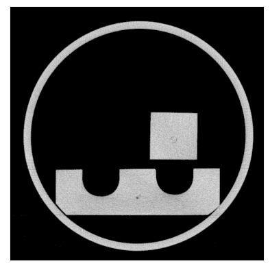
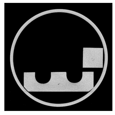
Figure 1: Test 1: STEMPO test problem. True images (first row) and sinograms (second row) from left to right at time instances $j=0,6,13,19$, respectively.

In this example we investigate STBP, STGP and time-uncorrelated prior models on a simulated dynamic tomography reconstruction problem. In particular, we consider the Spatio-TEmporal Motor-POwered (STEMPO) ground truth phantom from [25],
stempo_ground_truth_2d_b4.mat that contains 360 images. From the dataset we obtain $J=20$ images of size $560\times 560$ chosen uniformly from $1$ to $360$ with a factor of $8$, i.e., we choose the $1$st, the $8$th, the $16$th up to the $360$th image that represent the truth at $20$ time instances. Using the ASTRA toolbox [61] we generate the forward operators ${\mathcal{G}}_{j}$, $j=1,2,\dots,J$ by considering $J$ vectors of length $11$ containing projection angles. Each angles vector is generated by choosing $11$ equispaced degree angles from $(5*(j-1),5*(j-1)+140)$, for $j=1,2,\dots,J$ that are then converted to radian. Throughout the paper we denote the number of angles used to generate the forward problem with $n_{a}$. For this example we set $n_{a}=20$.

$j=0$

$j=6$

$j=13$

$j=19$

Figure 2: Reconstruction results of dynamic STEMPO test problem in the whitened space. Row from top to bottom: MAP for STBP ($q=1,p=1$), MAP for STGP ($q=2,p=2$) and MAP for time-uncorrelated model. Left to right: time step $j=0,6,13,19$.

We report the other parameters to generate the forward operators with ASTRA as follows. We choose origin to detector distance (detector_origin) to be $3*n_{x}$, the source to origin distance (source_origin) to be $n_{x}$, and the detector pixel size to be computed as $\frac{(\text{source\_origin}+\text{detector\_origin})}{\text{source\_origin}}$. Each forward operator ${\mathcal{G}}_{j}\in\mathbb{R}^{8701\times 313600}$ and the large operator can be represented by a blockdiagonal matrix $\overline{{\mathcal{G}}}=\operatorname{diag}({\mathcal{G}}_{1},\cdots{\mathcal{G}}_{j})\in\mathbb{R}^{174020\times 6272000}$. We apply the forward operators ${\mathcal{G}}_{j}$, to the $j-th$ true images $u^{\rm true}({\bf X},t_{j}))$, to obtain $J$ sinograms $y_{j}\in\mathbb{R}^{8701}$, with ${\bf Y}_{j}\in\mathbb{R}^{791\times 11}$, for $j=1,2,\dots,J$. We assume that the noise vector follows a multivariate normal Gaussian distribution with mean zero and covariance ${\bm{\Gamma}_{\rm noise}}$, i.e., ${\bf e}\sim\mathcal{N}(\bf{0},{\bm{\Gamma}_{\rm noise}})$. We perturb each measured vectorized sinogram $y^{\rm true}_{j}$ with white Gaussian noise, i.e., the noise vector $\varepsilon_{j}$ has mean zero and a rescaled identity covariance matrix (i.e., ${\Gamma}_{\rm noise}={\bf I}$, where ${\bf I}\in\mathbb{R}^{313600\times 313600}$). We refer to the ratio $\sigma_{j}=\|\varepsilon_{j}\|_{2}/\|{\mathcal{G}}_{j}\left(u^{\rm true}({\bf X},t_{j}))\right)\|_{2}$ as the noise level. The true images $u^{\rm true}({\bf X},t_{j}))$ at time steps $j=0,6,13,19$ are shown in the first rows of Figure 1. Observed noisy sinograms are shown in the second row of Figure  1.

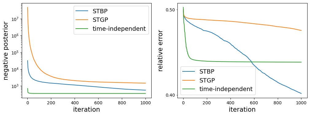
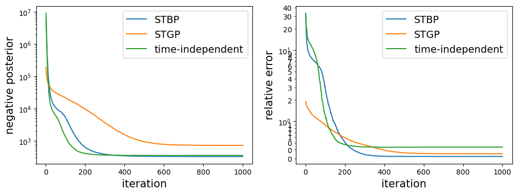
Figure 3: Dynamic STEMPO tomography: negative posterior densities and relative errors for the optimization in the original space (left) and in the whitened space (right) as functions of iterations in the BFGS algorithm used to obtain MAP estimates. Early termination is implemented if the error falls below some threshold or the maximal iteration (1000) is reached.

Table 1: MAP estimates of STEMPO by STBP, STGP and time-uncorrelated prior models. Relative error of MAP ($u^{*}$), RLE, log-likelihood, PSNR, SSIM, and HaarPSi measures. Standard deviations are obtained by repeating the experiments for 10 times with different random seeds.

	time-uncorrelated	STGP	STBP
RLE	0.4354 (2.91e-5)	0.3512(1.42e-4)	0.3217 (2.72e-5)
log-likelihood	-39190.72 (0.65)	-39085.37 (5.49)	-39697.93 (0.71)
PSNR	15.8250	18.7639	19.5753
SSIM	0.9916	0.9968	0.9977
HaarPSI	0.2751	0.4088	0.4983

We minimize negative log-posterior densities for the three models with STBP, STGP and time-uncorrelated priors to obtain the maximum a posterior (MAP) estimates. Figure 2 compares these MAP estimates obtained in the whitened space and mapped to the original space. With STBP, we have the sharpest reconstruction on the second row that is the closest to the truth. However, the results by the other two models are either blurry (by STGP on the third row) or noisy (by the time-uncorrelated model on the last row). Table 1 confirms that STBP model yields higher reconstruction quality with the lowest relative error. Though their log-likelihood values are not comparable in the regularized optimization, STBP achieves the lowest $\textrm{RLE}=32.17\%$ on average in 10 experiments repeated with different random seeds. Other reconstruction quality measures such as PSNR, SSIM, and HaarPSI are shown in 1, rows 3-5. Higher reconstruction quality observed in RLE is reflected by the other measures as well.

$j=0$

$j=6$

$j=13$

$j=19$

Figure 4: MCMC results of dynamic STEMPO test problem in the whitened space. Row from top to bottom: posterior mean for STBP ($q=1,p=1$), posterior standard deviation for STBP ($q=1,p=1$), posterior mean for STGP ($q=2,p=2$), and posterior standard deviation for STGP ($q=2,p=2$). Left to right: time step $t=0,6,13,19$.

On the other hand, the MAP estimates generated by these three models in the original space are illustrated in Figure 9. They are more than $40\%$ RLE’s and are generally more blurry than those obtained in the whitened space. Such difference can also be seen in Figure 3 where the objective functions and RLE’s are compared between the whiten space optimization (left two panels) and the original space optimization (right two panels) for these three models: optimization in the whitened space outputs better results with lower errors and fewer iterations. In general, STBP converges faster to the lowest error state among the three models.

Lastly, we apply the white-noise manifold infinite-dimensional MALA (wn-minfMALA) algorithm to sample the posterior samples for the two models with STBP and STGP priors respectively (the result for time-uncorrelated prior is far worse and hence omitted) and compare their posterior estimates in Figure 4. We generate 3000 samples and discard the first 1000 samples. The remaining 2000 samples are used to estimate the posterior means (the first and third rows) and posterior standard deviations (the second and the last rows). Due to the large dimensionality ($560\times 560\times 20$) and limited number of samples, these posterior estimates tend to be noisy. The posterior mean estimates are not good reconstructions as their MAP estimates. Yet the posterior standard deviations by STBP (the second row) provides more clear uncertainty information compared with those by STGP model (the last row).

6.2 Emoji Tomography Reconstruction

In this example, we test our methods on real data of an “emoji” phantom measured at the University of Helsinki [45]. The forward operator and the data can be obtained from the file DataDynamic_128x30.mat. The available data represents $J=33$ time steps of a series of the X-ray sinogram of emojis made of small ceramic stones obtained by shining $217$ projections from $n_{a}=10$ angles.

$j=6$

$j=14$

$j=22$

$j=30$

Figure 5: Test 2: Emoji test problem. Setup images (first row) and sinograms (second row) from left to right at time instances $j=6,14,22,30$, respectively.

We are interested in reconstructing a sequence of images $u({\bf X},t_{j})$, $j=0,1,\dots,32$, of size $n_{x}\times n_{y}$, where $n_{x}=n_{x}=128$, from low-dose observations measured from a limited number of angles $n_{a}$. Hence, the unknown images are collected in $u\in{\mathbb{R}}^{540,672}$, with $u=\left[(u({\bf X},t_{0})^{T},\\ u({\bf X},t_{1})^{T},\\ \dots\\ ,u({\bf X},t_{32})^{T}\right]^{T}$ representing the dynamic sequence of the emoji changing from an expressionless face with closed eyes and a straight mouth to a face with smiling eyes and mouth, where the outmost circular shape does not change. We refer to Figure 5 for a sample of 4 setup images (first row) and sinograms (second row) at time steps $j=6,14,22,30$. The low-dose available observations can be modeled by the measurement matrix ${\mathcal{G}}$ which describes the forward model of the Radon transform that represents line integrals. In this case, we have blockdiagonal matrix with 33 blocks. Although the ground truth is not available, we can qualitatively compare the visual results.

$j=6$

$j=14$

$j=22$

$j=30$

Figure 6: Reconstruction results for the emoji problem with $n_{a}=10$ in the whitened space. Row from top to bottom: MAP for STBP ($q=1,p=1$), MAP for STGP ($q=2,p=2$) and MAP for time-uncorrelated model. Left to right: time step $t=6,14,22,30$.

Figure 6 compares the MAP estimates by STBP (the second row), STBP (the third row) and the time-uncorrelated (the last row) prior models in the whitened space. Again we observe similar advantage in reconstructing a sequence of sharper tomography images by STBP compared with those more blurry results by STGP. Note, by ignoring the temporal correlation, the time-uncorrelated prior model yields reconstruction images that are difficult to recognize.

We also compare the UQ results generated by white-noise manifold MALA for the two models, STBP and STGP, respectively in Figure 11. Again we observe noisy posterior mean estimates for both models. However, the posterior standard deviation estimates by STBP are slightly clearer than those by STGP in characterizing the uncertainty field representing the changing smiling faces.

6.3 Navier-Stokes Inverse Problem

Lastly, we consider a complex non-linear inverse problem involving the following 2-d Navier-Stokes equation (NSE) for a viscous, incompressible fluid in vorticity form on the unit torus:

$$\begin{split}\partial_{t}w(x,t)+u(x,t)\cdot\nabla w(x,t)&=\nu\Delta w(x,t)+f(x),\qquad x\in(0,1)^{2},t\in(0,T]\\ \nabla\cdot u(x,t)&=0,\qquad\qquad\qquad\qquad\quad x\in(0,1)^{2},t\in[0,T]\\ w(x,0)&=w_{0}(x),\qquad\qquad\qquad\quad x\in(0,1)^{2}\end{split}$$ (36)

where $u\in C([0,T];H^{r}_{\text{per}}((0,1)^{2};\mathbb{R}^{2}))$ for any $r>0$ is the velocity field, $w=\nabla\times u$ is the vorticity, $w_{0}\in L^{2}_{\text{per}}((0,1)^{2};\mathbb{R})$ is the initial vorticity, $\nu\in\mathbb{R}_{+}$ is the viscosity coefficient, and $f\in L^{2}_{\text{per}}((0,1)^{2};\mathbb{R})$ is the forcing function.

Because NSE is well-known computationally intensive to solve, we follow [43, 35] to build an emulator based on the Fourier operator neural network (FNO) that maps the vorticity up to time 10 to the vorticity up to some later time $T>10$:

$${\mathcal{G}}^{\dagger}: C([0,10];H^{r}_{\text{per}}((0,1)^{2};\mathbb{R}^{2}))\to C((10,T];H^{r}_{\text{per}}((0,1)^{2};\mathbb{R}^{2})),$$ (37)

$$w|_{(0,1)^{2}\times[0,10]}\mapsto w|_{(0,1)^{2}\times(10,T]}$$

One of the outstanding features of FNO is that the neural network is built to learn operators defined on function spaces. Compared with traditional neural networks for simulating PDE solutions including CNN, PINNs, ResNet etc, FNO is mesh-independent and very efficient for the inference of Bayesian inverse problem constrained by NSE.

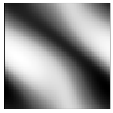
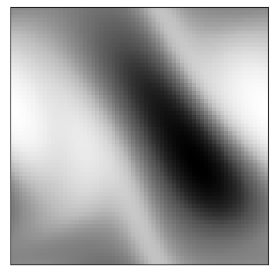
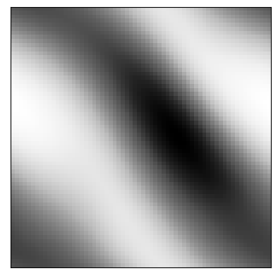
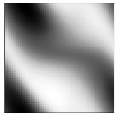
Figure 12: Observed and emulated Navier-Stokes equation solutions. Upper row: true NSE trajectory solved by classical PDE solver; Lower row: emulated NSE trajectory by FNO. Left to right: time step $t=30,36,42,48,54$.

In this example, we choose the viscosity $\nu=1\mathrm{e}-3$ and set $T=30$. Since the target operator, ${\mathcal{G}}^{\dagger}$, is time-dependent, we train a 3-d FNO (FNO-3d) based on 5000 pairs of input vorticity (for the first 10 seconds) and output vorticity (for the following 30 seconds) solved on $64\times 64$ spatial mesh using the network configuration as in [43]. We initialize the vorticity $w_{0}$ with a (star-convex) polygon shown as in the top left of Figure 7 which also demonstrates a few snapshots of true vorticity trajectory, $u^{\dagger}=w^{\dagger}|_{(0,1)^{2}\times[0,10]}$, at $t=0,3,6,9$ in the first row. Figure 12 compares the true NSE trajectory solved by the classical PDE solver (upper row) and the emulated trajectory by FNO network (lower row). The visual difference is hard to discern. We observe data of vorticity $w|_{(0,1)^{2}\times(10,30]}$ based on the true initial input $w^{\dagger}|_{(0,1)^{2}\times[0,10]}$, with Gaussian noise contamination, i.e. $y={\mathcal{G}}(w^{\dagger}|_{(0,1)^{2}\times[0,10]})+\eta$ with $\eta\sim N(0,\sigma^{2}_{\eta})$.

$j=0$

$j=3$

$j=6$

$j=9$

Figure 7: Inverse solutions of Navier-Stokes equation in the whitened space. Row from top to bottom: True NSE trajectories, MAP for STBP ($q=1,p=1$), MAP for STGP ($q=2,p=2$) and MAP for time-uncorrelated model. Left to right: time step $t=0,3,6,9$.

Unlike the traditional time-dependent inverse problems seeking the solution of initial condition $w_{0}$ alone, we are interested in the inverse solution of vorticity for an initial period, i.e. $w|_{(0,1)^{2}\times[0,10]}$. What is more, we want to obtain UQ for such spatiotemporal object in addition to its point estimate (MAP) using STBP, STGP and time-uncorrelated priors. Their point solutions as MAP estimates are compared in Figure 7. Note, this inverse problem for a spatiotemporal solution is much more challenging than the traditional inverse problem for just the initial condition based on the same amount of downstream observations. STBP still yields the inverse solution (the second row) closest to the true trajectory among the three models. Note, due to the lack of temporal correlation, the time-uncorrelated prior model gives a solution trajectory that is very jumpy. Table 2 further confirms that STBP prior model yields the best inverse solution with the lowest RLE, $66.18\%$, compared with the true trajectory, almost $10\%$ lower than the other two methods. Figure 8 compares the optimization objective function, the negative log-posterior and the relative error as functions of iterations. STBP could converge to lower RLE value, while STGP terminates earlier at higher RLE value.

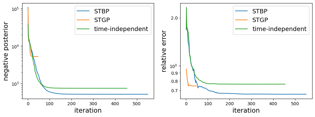
Figure 8: Navier-Stokes inverse problem: negative posterior densities (left) and relative errors (right) for the optimization in the whitened space as functions of iterations in the BFGS algorithm used to obtain MAP estimates. Early termination is implemented if the error falls below some threshold or the maximal iteration (1000) is reached.

Table 2: MAP estimates of NSE trajectory by STBP, STGP and time-uncorrelated prior models. Relative error of MAP ($u^{*}$), $\textrm{RLE}:=\|u^{*}-u^{\dagger}\|/\|u^{\dagger}\|$, log-likelihood, PSNR, SSIM, and HaarPSi measures. Standard deviations are obtained by repeating the experiments for 10 times with different random seeds.

	time-uncorrelated	STGP	STBP
RLE	0.77 (8.633e-05)	0.75 (4.471e-05)	0.66 (0.)
log-lik	-229.3 (0.18)	-1585.97 (0.357)	-173.33 (0.09)
PSNR	15.73 (0.001)	15.96 (0.001)	16.99 (0.002)
SSIM	0.18 (0.)	0.22 (7.648e-05)	0.34 (0.)
HaarPSI	1.0 (1.347e-06)	1.0 (5.799e-07)	1.0 (1.487e-06)

Lastly, because of the computational cost, we apply white-noise infinite-dimensional HMC (wn-infHMC) instead of wn-minfMALA for the UQ. We run 20,000 iterations, discard the first 5,000, and sub-sample every one of three. The remaining 5,000 samples are used to obtain posterior estimates illustrated in Figure 13 comparing STBP model (the first two rows) against STGP model (the last two rows). The posterior mean by STBP (the first row) is more noisy compared with that by STGP (the thrid row). However the posterior standard deviation by STBP (the second row) is more informative than that of STGP (the last row).

7 Conclusion

In this paper we propose a computational framework for Bayesian inverse problems to construct spatiotemporal solutions. We generalize series based Besov measure for spatial functions to a nonparametric prior for spatiotemporal functions, hence named spatiotemporal Besov process (STBP). We make use of the recently proposed $Q$-exponential process [37] to replace the univariate $q$-exponential random variables in the series defining Besov process in order to capture the temporal correlations of multiple images. The proposed STBP simultaneously model the inhomogeneity in space and correlation in time in the spatiotemporal target of Bayesian invers propblems.

To address the challenges in high-dimensional posterior sampling with non-Gaussian priors, we take advantage of the existing literature of dimension-independent MCMC algorithms for Gaussian priors and propose a white-noise representation of the STBP. The derived white-noise MCMC provides robust and efficient inference for Bayesian models with STBP priors.

Through extensive numerical experiments from computerized tomography with simulated and real data and PDE-governed inverse problems we show that spatiotemporal Besov priors with a proper chosen covariance kernel outperform the priors with uncorrelated time and yield higher quality reconstructions with edges well-preserved compared to the spatiotemporal Gaussian priors while reducing the posterior uncertainty. Such promising results from real computerized tomography and limited angle data suggest the potential applications in medical imaging analysis.

Appendix

More Numerical Results

$j=0$

$j=6$

$j=13$

$j=19$

Figure 9: Reconstruction results of dynamic STEMPO test problem. Row from top to bottom: MAP for $q=1,p=1$, MAP for $q=2,p=2$ and MAP $q=1,p=1$ without time correlation. Left to right: time step $t=0,6,13,19$.

$j=6$

$j=14$

$j=22$

$j=30$

Figure 10: Reconstruction results for the emoji problem with $n_{a}=10$. Row from top to bottom: MAP for STBP ($q=1,p=1$), MAP for STGP ($q=2,p=2$) and MAP for time-uncorrelated model. Left to right: time step $t=6,14,22,30$.

$j=6$

$j=14$

$j=22$

$j=30$

Figure 11: MCMC results of the emoji problem with $n_{a}=10$ in the whitened space. Row from top to bottom: posterior mean for STBP ($q=1,p=1$), posterior standard deviation for STBP ($q=1,p=1$), posterior mean for STGP ($q=2,p=2$), and posterior standard deviation for STGP ($q=2,p=2$). Left to right: time step $t=6,14,22,30$.

$j=0$

$j=6$

$j=12$

$j=18$

$j=24$

$j=0$

$j=3$

$j=6$

$j=9$

Figure 13: Bayesian inverse solutions of Navier-Stokes equation in the whitened space. Row from top to bottom: posterior mean for STBP ($q=1,p=1$), posterior standard deviation for STBP ($q=1,p=1$), posterior mean for STGP ($q=2,p=2$), and posterior standard deviation for STGP ($q=2,p=2$). Left to right: time step $t=0,3,6,9$.

References

• [1] Anatolii Borisovich Bakushinskii. A general method of constructing regularizing algorithms for a linear incorrect equation in hilbert space. Zhurnal Vychislitel’noi Matematiki i Matematicheskoi Fiziki, 7(3):672–677, 1967.
• [2] A. Beskos, F. J. Pinski, J. M. Sanz-Serna, and A. M. Stuart. Hybrid Monte-Carlo on Hilbert spaces. Stochastic Processes and their Applications, 121:2201–2230, 2011.
• [3] Alexandros Beskos. A stable manifold MCMC method for high dimensions. Statistics & Probability Letters, 90:46–52, 2014.
• [4] Alexandros Beskos, Mark Girolami, Shiwei Lan, Patrick E. Farrell, and Andrew M. Stuart. Geometric MCMC for infinite-dimensional inverse problems. Journal of Computational Physics, 335, 2017.
• [5] Alexandros Beskos, Gareth Roberts, Andrew Stuart, and Jochen Voss. MCMC methods for diffusion bridges. Stochastics and Dynamics, 8(03):319–350, 2008.
• [6] Tan Bui-Thanh and Omar Ghattas. A scalable algorithm for map estimators in bayesian inverse problems with Besov priors. Inverse Problems & Imaging, 9(1):27, 2015.
• [7] D. Calvetti and E. Somersalo. An Introduction to Bayesian Scientific Computing: Ten Lectures on Subjective Computing, volume 2. Springer Science & Business Media, 2007.
• [8] Daniela Calvetti, Monica Pragliola, Erkki Somersalo, and Alexander Strang. Sparse reconstructions from few noisy data: analysis of hierarchical Bayesian models with generalized gamma hyperpriors. Inverse Problems, 36(2):025010, 2020.
• [9] Daniela Calvetti and Erkki Somersalo. Bayesian image deblurring and boundary effects. In Advanced Signal Processing Algorithms, Architectures, and Implementations XV, volume 5910, pages 281–289. SPIE, 2005.
• [10] Daniela Calvetti and Erkki Somersalo. Inverse problems: From regularization to Bayesian inference. Wiley Interdisciplinary Reviews: Computational Statistics, 10(3):e1427, 2018.
• [11] Stamatis Cambanis, Steel Huang, and Gordon Simons. On the theory of elliptically contoured distributions. Journal of Multivariate Analysis, 11(3):368–385, 1981.
• [12] Robert H Cameron and William T Martin. Transformations of weiner integrals under translations. Annals of Mathematics, pages 386–396, 1944.
• [13] M Cardiff and PK Kitanidis. Bayesian inversion for facies detection: An extensible level set framework. Water Resources Research, 45(10), 2009.
• [14] Carlos M Carvalho, Nicholas G Polson, and James G Scott. The horseshoe estimator for sparse signals. Biometrika, 97(2):465–480, 2010.
• [15] George Casella, Malay Ghosh, Jeff Gill, and Minjung Kyung. Penalized regression, standard errors, and Bayesian Bassos. Bayesian analysis, 5(2):369–411, 2010.
• [16] Victor Chen, Matthew M Dunlop, Omiros Papaspiliopoulos, and Andrew M Stuart. Dimension-robust mcmc in bayesian inverse problems. arXiv preprint arXiv:1803.03344, 2018.
• [17] Simon L Cotter, Massoumeh Dashti, James Cooper Robinson, and Andrew M Stuart. Bayesian inverse problems for functions and applications to fluid mechanics. Inverse problems, 25(11):115008, 2009.
• [18] Simon L Cotter, Gareth O Roberts, AM Stuart, and David White. MCMC methods for functions: modifying old algorithms to make them faster. Statistical Science, 28(3):424–446, 2013.
• [19] Masoumeh Dashti, Stephen Harris, and Andrew Stuart. Besov priors for Bayesian inverse problems. arXiv preprint arXiv:1105.0889, 2011.
• [20] Masoumeh Dashti and Andrew M. Stuart. The Bayesian Approach to Inverse Problems, pages 311–428. Springer International Publishing, Cham, 2017.
• [21] Matthew M Dunlop and Andrew M Stuart. Map estimators for piecewise continuous inversion. Inverse Problems, 32(10):105003, 2016.
• [22] Heinz Werner Engl, Martin Hanke, and Andreas Neubauer. Regularization of inverse problems, volume 375. Springer Science & Business Media, 1996.
• [23] Gene H Golub, Per Christian Hansen, and Dianne P O’Leary. Tikhonov regularization and total least squares. SIAM journal on matrix analysis and applications, 21(1):185–194, 1999.
• [24] Per Christian Hansen. Discrete inverse problems: insight and algorithms. SIAM, 2010.
• [25] Tommi Heikkilä. Stempo–dynamic X-ray tomography phantom. arXiv preprint arXiv:2209.12471, 2022.
• [26] Bamdad Hosseini and Nilima Nigam. Well-posed Bayesian inverse problems: priors with exponential tails. SIAM/ASA Journal on Uncertainty Quantification, 5(1):436–465, 2017.
• [27] Marco A Iglesias, Yulong Lu, and Andrew M Stuart. A bayesian level set method for geometric inverse problems. Interfaces and free boundaries, 18(2):181–217, 2016.
• [28] Valentin Konstantinovich Ivanov. On linear problems which are not well-posed. In Doklady akademii nauk, volume 145, pages 270–272. Russian Academy of Sciences, 1962.
• [29] Bangti Jin, Peter Maaß, and Otmar Scherzer. Sparsity regularization in inverse problems. Inverse Problems, 33(6), 2017.
• [30] Mark E. Johnson. Multivariate Statistical Simulation, chapter 6 Elliptically Contoured Distributions, pages 106–124. Probability and Statistics. John Wiley & Sons, Ltd, 1987.
• [31] Jari Kaipio and Erkki Somersalo. Statistical and computational inverse problems, volume 160. Springer Science & Business Media, 2006.
• [32] Jari P Kaipio and Erkki Somersalo. Statistical inversion theory. Statistical and Computational Inverse Problems, pages 49–114, 2005.
• [33] W Clem Karl. Regularization in image restoration and reconstruction. In Handbook of Image and Video Processing, pages 183–V. Elsevier, 2005.
• [34] Bartek T Knapik, Aad W Van Der Vaart, and J Harry van Zanten. Bayesian inverse problems with gaussian priors. The Annals of Statistics, 39(5):2626–2657, 2011.
• [35] Nikola Kovachki, Zongyi Li, Burigede Liu, Kamyar Azizzadenesheli, Kaushik Bhattacharya, Andrew Stuart, and Anima Anandkumar. Neural operator: Learning maps between function spaces. 08 2021.
• [36] Shiwei Lan. Adaptive dimension reduction to accelerate infinite-dimensional geometric markov chain monte carlo. Journal of Computational Physics, 392:71 – 95, September 2019.
• [37] Shiwei Lan, Shuyi Li, and Michael O’Connor. Bayesian regularization on function spaces via q-exponential process. 10 2022.
• [38] Matti Lassas, Eero Saksman, and Samuli Siltanen. Discretization-invariant bayesian inversion and besov space priors. Inverse Problems and Imaging, 3(1):87–122, 2009.
• [39] Matti Lassas and Samuli Siltanen. Can one use total variation prior for edge-preserving Bayesian inversion? Inverse Problems, 20(5):1537, 2004.
• [40] J Lee and PK Kitanidis. Bayesian inversion with total variation prior for discrete geologic structure identification. Water Resources Research, 49(11):7658–7669, 2013.
• [41] David Leporini and J-C Pesquet. Bayesian wavelet denoising: Besov priors and non-Gaussian noises. Signal processing, 81(1):55–67, 2001.
• [42] Qing Li and Nan Lin. The Bayesian elastic net. Bayesian analysis, 5(1):151–170, 2010.
• [43] Zongyi Li, Nikola Borislavov Kovachki, Kamyar Azizzadenesheli, Burigede liu, Kaushik Bhattacharya, Andrew Stuart, and Anima Anandkumar. Fourier neural operator for parametric partial differential equations. In International Conference on Learning Representations, 2021.
• [44] Markku Markkanen, Lassi Roininen, Janne MJ Huttunen, and Sari Lasanen. Cauchy difference priors for edge-preserving Bayesian inversion. Journal of Inverse and Ill-posed Problems, 27(2):225–240, 2019.
• [45] Alexander Meaney, Zenith Purisha, and Samuli Siltanen. Tomographic x-ray data of 3d emoji. arXiv preprint arXiv:1802.09397, 2018.
• [46] R. M. Neal. MCMC using Hamiltonian dynamics. In S. Brooks, A. Gelman, G. Jones, and X. L. Meng, editors, Handbook of Markov Chain Monte Carlo. Chapman and Hall/CRC, 2010.
• [47] Bernt Øksendal. Stochastic Differential Equations. Springer Berlin Heidelberg, 2003.
• [48] Trevor Park and George Casella. The Bayesian Lasso. Journal of the American Statistical Association, 103(482):681–686, 2008.
• [49] Nicholas G. Polson, James G. Scott, and Jesse Windle. The Bayesian Bridge. Journal of the Royal Statistical Society Series B: Statistical Methodology, 76(4):713–733, 11 2013.
• [50] William Reese, Arvind K Saibaba, and Jonghyun Lee. Bayesian level set approach for inverse problems with piecewise constant reconstructions. arXiv preprint arXiv:2111.15620, 2021.
• [51] Rafael Reisenhofer, Sebastian Bosse, Gitta Kutyniok, and Thomas Wiegand. A Haar wavelet-based perceptual similarity index for image quality assessment. Signal Processing: Image Communication, 61:33–43, 2018.
• [52] Uwe Schmidt, Kevin Schelten, and Stefan Roth. Bayesian deblurring with integrated noise estimation. In CVPR 2011, pages 2625–2632. IEEE, 2011.
• [53] I. J. Schoenberg. Metric spaces and completely monotone functions. Annals of Mathematics, 39:811–841, 1938.
• [54] Roel Snieder and Jeannot Trampert. Inverse problems in geophysics. In Wavefield inversion, pages 119–190. Springer, 1999.
• [55] Scott A Starks and Vladik Kreinovich. Multispectral inverse problems in satellite image processing. In Bayesian Inference for Inverse Problems, volume 3459, pages 138–146. SPIE, 1998.
• [56] Andrew M Stuart. Inverse problems: a Bayesian perspective. Acta Numerica, 19:451–559, 2010.
• [57] Luis Tenorio. Statistical regularization of inverse problems. SIAM review, 43(2):347–366, 2001.
• [58] Andrey Nikolayevich Tikhonov. On the stability of inverse problems. In Dokl. Akad. Nauk SSSR, volume 39, pages 195–198, 1943.
• [59] Hans Triebel. Function spaces and wavelets on domains. Number 7. European Mathematical Society, 2008.
• [60] Felipe Uribe, Yiqiu Dong, and Per Christian Hansen. Horseshoe priors for edge-preserving linear Bayesian inversion. arXiv preprint arXiv:2207.09147, 2022.
• [61] Wim Van Aarle, Willem Jan Palenstijn, Jan De Beenhouwer, Thomas Altantzis, Sara Bals, K Joost Batenburg, and Jan Sijbers. The ASTRA Toolbox: A platform for advanced algorithm development in electron tomography. Ultramicroscopy, 157:35–47, 2015.
• [62] L Verlet and D Levesque. On the theory of classical fluids VI. Physica, 36(2):254–268, 1967.
• [63] Curtis R Vogel. Computational methods for inverse problems. SIAM, 2002.
• [64] Zhou Wang, Alan C Bovik, Hamid R Sheikh, and Eero P Simoncelli. Image quality assessment: From error visibility to structural similarity. IEEE transactions on image processing, 13(4):600–612, 2004.
• [65] Kehe Zhu. Operator theory in function spaces. Number 138. American Mathematical Soc., 2007.