PTArcade
v0.1.0

Abstract

This is a lightweight manual for PTArcade, a wrapper of ENTERPRISE and ceffyl that allows for easy implementation of new-physics searches in PTA data. In this manual, we describe how to get PTArcade installed (either on your local machine or an HPC cluster). We discuss how to define a stochastic or deterministic signal and how PTArcade implements these signals in PTA-analysis pipelines. Finally, we show how to handle and analyze the PTArcade output using a series of utility functions that come together with PTArcade.

1 Introduction

The detection of gravitational waves (GWs) by the LIGO and VIRGO collaborations [1] heralds the beginning of GW astronomy. The extremely weak interaction between GWs and matter makes them ideal probes for dense astrophysical and cosmological environments, one relevant example being the pre-recombination Universe. This epoch in the cosmological evolution is characterized by high densities of charged particles, which makes it opaque to electromagnetic radiation. However, any gravitational-wave signal produced during this epoch would propagate essentially unimpeded over cosmic distances to be measured today. Detecting a primordial GW signal will then provide a direct glimpse into the primordial Universe and potentially allow us to test beyond Standard Model (BSM) physics, where the production of primordial GWs is a ubiquitous feature [2, 3, 4].

Recently, several pulsar timing array (PTA) collaborations have found convincing evidence for a gravitational wave background (GWB) in the nanohertz band (see for example reference [5]). The origin of this background is still unknown, and while supermassive black hole binaries (SMBHBs) remain the primary suspect [6, 7, 8, 9, 10, 11], a primordial origin is also a viable explanation at this stage. The recent NANOGrav search for new-physics signals [12] has considered several BSM models that could generate a primordial GWB compatible with the one observed in the NANOGrav 15yr dataset. However, many models remain to be tested.

In this work, we present PTArcade, a wrapper of ENTERPRISE [13, 14] and ceffyl [15]. PTArcade aims to provide an accessible way to perform Bayesian analyses of new-physics signals with PTA data. The user can either specify the signal by providing the GW energy density spectrum as a fraction of the closure density $\Omega_{\mathrm{GW}}(f;\,\vec{\theta})$ (in case of GWB signals) or the signal time series $h(t,\vec{\theta})$ (in case of deterministic signals). Here, $\vec{\theta}$ is an array containing all the model parameters characterizing the new-physics signal for which PTArcade will allow to derive posterior probability distributions and upper limits.

Users can specify their models by using simple Python files, which allows for great flexibility and allows to specify signals either analytically or using tabulated data. PTArcade is shipped with sensible default settings that closely resemble official PTA analyses, but users may override them on a case-by-case basis through a pure-Python configuration file.

While all the necessary information needed to install and run PTArcade can be found in this manual, more details and examples can be found in the PTArcade documentation web page.

2 Quick Start

The first step consists in installing PTArcade. The easiest way to do this is to use the Python package manager conda. Simply download this environment file, open a terminal, and type

⬇

conda env create -f ptarcade.yml

If everything went smoothly, great, PTArcade is now installed on your machine and you can start using it!

To guide our discussion, we will consider a toy model: Suppose you have a model that produces a GWB with a broken power-law spectrum of the form

$$h^{2}\Omega_{\scriptscriptstyle\mathrm{GW}}(f;A_{*},f_{*})=A_{*}\left(\frac{f_{*}}{f}+\frac{f}{f_{*}}\right)^{-1}\,,$$ (1)

and you want to know for what values of the parameters $A_{*}$ and $f_{*}$ this GWB can reproduce the signal observed in the NG15 data. The first step is to create, what we call, a model file. This is a simple Python file that contains the definition of the GWB spectral shape and the prior distributions for the model parameters. For the GWB from our example, the model file is:

A Typical Model File

⬇

from ptarcade.models_utils import prior

parameters = {’log_A_star’ : prior("Uniform", -14, -6),

’log_f_star’ : prior("Uniform", -10, -6)} ➊0.0pt

def S(x):

return 1 / (1/x + x)

def spectrum(f, log_A_star, log_f_star): ➋0.0pt

A_star = 10**log_A_star

f_star = 10**log_f_star

return A_star * S(f/f_star)

In general, the model file for a GWB signal needs to contain the following two things:

• parameters: This variable has to be assigned to a dictionary whose keys are strings corresponding to the model parameters’ names and whose values are the parameters’ priors. The prior distributions can be specified using the prior function from the models_utils module. The syntax for this function is the following: The first argument that is passed to this function is a string specifying the prior type. The subsequent arguments are the parameters describing the prior. By default, the parameters are assumed to be common across all pulsars in the array. If you want a parameter to be pulsar dependent, you need to add the flag common=False when instantiating the prior object.

  In our example, we have chosen the names log_A_star and log_f_star for the parameters $\log_{10}A_{*}$ and $\log_{10}(f_{*}/{\textrm{H}z})$. For both, we have chosen uniform priors with the ranges $[-14,-6]$ and $[-10,-6]$, respectively.

• spectrum(f, ...): this function specifies the GWB spectrum. Its first parameter should be named f, and it has to be a NumPy array containing the frequencies (in units of Hz) at which the spectrum is evaluated. The names of the remaining parameters should match the ones defined in the parameters dictionary (in our case log_A_star and log_f_star). The spectrum function should return a NumPy array with the same dimensions as f and contain the value of $h^{2}\Omega_{\scriptscriptstyle\mathrm{GW}}$ at each of the frequencies in f.

Once you have created the model file, you are ready to run PTArcade. To proceed, open a terminal window and type the following:

⬇

1ptarcade -m ./model_file.py

The argument passed to the -m input flag is supposed to be the path to the model file. By default, PTArcade will output a chain of Markov Chain Monte Carlo samples (together with other files discussed in the next section) to the directory ./chains/np_model/chain_0. This chain of MC samples can then be used to derive the posterior distribution for the parameters of the user-specified signal.

Once the sampling of the chains is complete, you can use one of the many market-available tools to produce posterior-distribution plots. Two popular choices are corner [16] and GetDist [17]. PTArcade itself provides two modules, chains_utils and plot_utils, that can be used to help in this procedure (see section 3.6). When using these two modules, producing the posterior plots can be done with only a few lines of code:

Loading Chains and Parameter Files

⬇

import ptarcade.plot_utils as p_utils

import ptarcade.chains_utils as c_utils

chain, params = c_utils.import_chains(’./chains/np_model/’) ➌0.0pt

p_utils.plot_posteriors([chain] , [params]) ➍0.0pt

In 2, we use the function import_chains to load the MCMC chains and the parameter files of the run. This function takess the path to a folder containing the chains and loads them into a NumPy array. Additionally, it returns a dictionary containing the names of the model parameters as keys and a list with the parameters’ prior ranges as values. The plot_posteriors function in 2 produces a plot with the 2D and 1D marginalized posteriors for the parameters of our model. For the example at hand, we obtain the plot which is shown in Figure 1. Details on how to control the appearance of this plot are provided in Section 3.6.

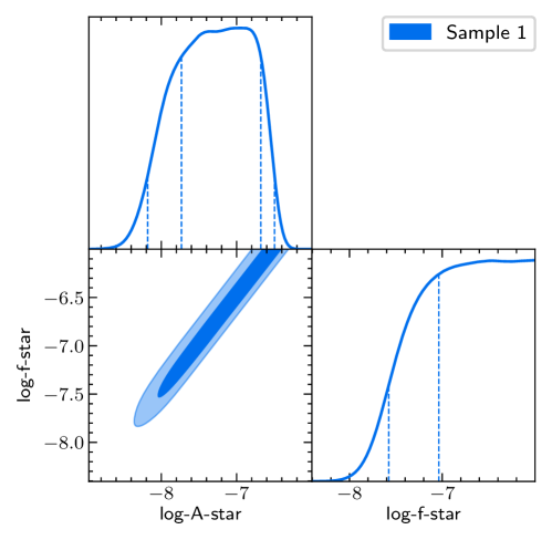
Figure 1: Reconstructed posterior distributions for the parameters of the example GWB described in Eq. (1). On the diagonal of the corner plot, we report the 1D marginalized distributions together with the $68\%$ and $95\%$ Bayesian credible intervals (vertical lines), while the off-diagonal panels show the $68\%$ (darker) and $95\%$ (lighter) Bayesian credible regions in the 2D posterior distributions. We construct all credible intervals and regions by integrating over the regions of highest posterior density.

3 More Details

In this section, we provide more details on the installation procedure (Section 3.1), how to run PTArcade (Section 3.2), how PTArcade implements user-specified signals in PTAs analysis pipelines (Section 3.3), how to personalize a PTArcade run by using model and configuration files (Section 3.5), the structure of the output data (Section 3.4), and the content of the utility modules (Section 3.6). Throughout this section, user-controllable parameters will be highlighted in green and hyperlinked to the relevant discussion in the model or configuration file sections.

3.1 Installation methods

If you are familiar with Python and want to install PTArcade on your local machine, we recommend doing so by using either conda or pip. If you are not familiar with Python or want to install PTArcade on a cluster, we recommend using a docker or a singularity container. In the following, we will discuss all these possible installation methods.

Conda installation recommended

The easiest way of installing PTArcade is via the Python package manager conda. We are in the process of submitting PTArcade to the conda forge-channel, and soon you will be able to install PTArcade as a conda package (refer to the "Installation section" of the PTArcade documentation web page for updates on this). In the meantime, you can install PTArcade using conda by downloading this environment file, and typing in a terminal

⬇

1conda env create -f ptarcade.yml

This will install PTArcade and all the required dependencies in a conda environment named ptarcade, and download the PTA data from the NANOGrav [18] and IPTA collaboration [19]. If you do not have conda installed on your machine, you should follow the instructions at this link.

PyPI installation

PTArcade is also released as a PyPI package and can be installed usingpip. However, the pip installation requires that non-Python dependencies are installed separately on your machine (or in a virtual environment). These dependencies are tempo2, SuiteSparse, and an MPI implementation. You can install these packages by typing the following in a terminal

• tempo2

  ⬇

  1curl -sSL https://raw.githubusercontent.com/vallis/libstempo/master/install_tempo2.sh | sh

• suite-sparse

  ⬇

  1# on mac

  2brew install suite-sparse

  3

  4# on debian

  5sudo apt install libsuitesparse-dev

• MPI

  ⬇

  1# on mac

  2brew install open-mpi

  3

  4# on debian

  5sudo apt install libopenmpi-dev openmpi-bin

Once you have installed these dependencies, you can install PTArcade from a terminal by typing

⬇

1pip install ptarcade

This will install all necessary Python dependencies and download the PTA data from the NANOGrav and IPTA collaboration.

With Docker

PTArcade is also packaged as a Docker image—including its Python and non-Python dependencies. You can download the image from a terminal by typing

⬇

1docker pull ngnewphy/ptarcade:latest

With singularity

You create a Singularity image for PTArcade by typing in your terminal

⬇

1singularity pull ptarcade.sif docker://ngnewphy/ptarcade:latest

This will create a Singularity image and save it as ptarcade.sif in the current working directory.

3.2 Run PTArcade

If you have installed PTArcade with pip or conda, you can run PTArcade by opening a terminal and typing

⬇

1ptarcade -m ./model.py

Here, the argument passed to the -m input flag is the path to a model file (in this example we are passing a model file named model.py and located in the current directory). In addition to a model file, other two optional arguments can be passed when running PTArcade:

• A configuration file can be passed via the input flag -c. Configuration files allow the user to control several aspect of the run, including the PTA dataset used, the number of MC trials, etc. More details on configuration files can be found in Section 3.5.

• A string that will be appended to the MC chain folder. This can be useful if you are running multiple instances of PTArcade for the same model (which can help you to get faster convergence) and you want to use the same output directory for all of them. By default, the chains will be saved in ./chains/np_model/chain_0. Each of the three elements of this path can be controlled by the user. ./chains can be changed by using the out_dir parameter in the configuration file, np_model can be changed by using the name parameter in the model file, and chain_0 can be changed via the argument passed to the -n input flag of the ptarcade command. The argument passed to the -n flag will be appended to chain_, so that passing -n 42 will result in the output directory ./chains/np_model/chain_42.

Run PTArcade with Docker

The commands in Section 3.2 must be slightly modified to run within a Docker container. Docker does not mount any directories into the container by default. You must pass directories to mount inside the container using the syntax -v <source>:<destination>. In the example below, we assume that the only directories you will pass to the command line options of PTArcade are accessible from your current working directory.

⬇

1docker run -v $(pwd):$(pwd) -w $(pwd) -i -t ptarcade -m ./model.py

• -v tells Docker what to mount from the host computer and where to mount it in the container. Here, we mount the current working directory of the host into the container using its full path.

• -w sets the working directory of the container. In this case, it sets it to the current working directory that was just mounted.

• -i -t keeps STDIN open and allocates a pseudo-TTY

The ptarcade in the docker run command refers to the name of the Docker image. If you would like to run something else inside the container, then replace the PTArcade options with the program to run. For example, to run an interactive Bash shell

⬇

1docker run -v $(pwd):$(pwd) -w $(pwd) -i -t ptarcade bash

Run PTArcade with Singularity

As with Docker, the commands to run PTArcade must be slightly modified to run using Singularity. However, the commands are much simpler because Singularity will automatically mount your home directory inside the container. Using the ptarcade.sif file you created in Section 3.1, type into a terminal

⬇

1singularity run ptarcade.sif -m ./model.py

You can also pass another command to run. For example, to start a Jupyter notebook type

⬇

1singularity run ptarcade.sif jupyter notebook

If you want an interactive shell, run the following command

⬇

1singularity shell ptarcade.sif

3.3 Statistical tools and their implementation

In this section, we provide more details on the inner workings of PTArcade and the implementation of the user-specified input in ENTERPRISE or ceffyl.

The PTA likelihood

Searches for stochastic or deterministic signals with PTAs utilize the pulsars’ timing residuals, $\vec{\delta t}$, which measure the discrepancy between the observed times of arrival (TOAs) of the pulses and the TOAs predicted by the pulsar timing model [20, 21, 22]. Timing residuals receive contributions by any effect not captured in the timing models used to derive them. This includes not only instrumental and spin noise but also GWB signals and possible deterministic signals. Specifically, we model the timing residuals as the sum of white noise, red noise, and small errors in the fit to the timing-ephemeris parameter [23]:

$$\vec{\delta t}=\vec{n}+\bm{F}\,\vec{a}+\bm{M}\,\vec{\epsilon}\,.$$ (2)

The first term on the right-hand side of Eq. (2), $\vec{n}$, describes the white noise that is assumed to be left in each of the $N_{\textrm{TOA}}$ timing residuals after subtracting all known systematics. White noise is assumed to be a zero-mean normal random variable, fully characterized by its covariance. Following standard conventions [24, 25], PTArcade sets the parameters of this $N_{\textrm{TOA}}\times N_{\textrm{TOA}}$ covariance matrix to their maximum-posterior values as recovered from single-pulsar noise studies (see reference [26, 27] for NG12, [28] for NG15, and [29] for IPTA DR2).

The second term on the right-hand side of Eq. (2) describes time-correlated stochastic processes, including pulsar-intrinsic red noise and GWB signals. These processes are modeled using a Fourier basis of frequencies $i/T_{\textrm{obs}}$, where $i$ indexes the harmonics of the basis and $T_{\textrm{obs}}$ is the timing baseline, extending from the first to the last recorded TOA in the complete PTA data set. Since we are generally interested in processes that exhibit long timescale correlations, the expansion is truncated after $N_{f,\textrm{red}}$ frequency bins for the intrinsic red-noise component, and $N_{f,\scriptscriptstyle{\textrm{GWB}}}$ frequency bins for the GWB component. This set of $N_{f}$ sine–cosine pairs evaluated at the different observation times are contained in the Fourier design matrix, $\bm{F}$. The Fourier coefficients of this expansion, $\vec{a}$, are assumed to be normally-distributed random variables with zero mean and the covariance matrix, $\langle\vec{a}\vec{a}^{\textrm{T}}\rangle=\bm{\phi}$, given by

$$[\phi]_{(ak)(bj)}=\delta_{ij}\left(\Gamma_{ab}\Phi_{i}+\delta_{ab}\varphi_{a,i}\right).$$ (3)

Here, $a$ and $b$ index the pulsars, $i$ and $j$ index the frequency harmonics, and $\Gamma_{ab}$ is the GWB overlap reduction function, which describes average correlations between pulsars $a$ and $b$ as a function of their angular separation in the sky. For an isotropic and unpolarized GWB, $\Gamma_{ab}$ is given by the Hellings & Downs correlation [30], also known as “quadrupolar” or “HD” correlation.

The first term on the right-hand side of Eq. (3) parameterizes the contribution to the timing residuals induced by a GWB in terms of the model-dependent coefficients $\Phi_{i}$. These coefficients can be related to the GWB energy density per logarithmic frequency interval, $d\rho_{\scriptscriptstyle\textrm{GW}}/d\ln f$, as a fraction of the closure density, $\rho_{c}$, via [31]

$$h^{2}\Omega_{\scriptscriptstyle\textrm{GW}}(f)\equiv\frac{h^{2}}{\rho_{c}}\frac{d\rho_{\scriptscriptstyle\textrm{GW}}(f)}{d\ln f}=\frac{8\pi^{4}f^{5}}{H_{0}^{2}/h^{2}}\,\frac{\Phi(f)}{\Delta f}\,.$$ (4)

Here, $\Delta f=1/T_{\textrm{obs}}$ is the width of the $N_{f}$ frequency bins. $H_{0}$ is the present-day value of the Hubble rate, and $h$ is the reduced Hubble constant, $H_{0}=h\times 100\,\textrm{km}\,\textrm{s}^{-1}\,\textrm{Mpc}^{-1}$. Finally, $\Phi(f)$ determines the coefficients $\Phi_{i}$ in Eq. (3), i.e., $\Phi_{i}=\Phi\left(i/T_{\textrm{obs}}\right)$. PTArcade will build $h^{2}\Omega_{\scriptscriptstyle\textrm{GW}}$ from any spectrum function defined by the user in the model file, and, if smbhb=True, add to it the expected signal produced by SMBHBs. The latter is modeled as a power law of the form

$$h^{2}\Omega_{\scriptscriptstyle\textrm{GW}}(f)=\frac{2\pi^{2}A_{\scriptscriptstyle\textrm{BHB}}^{2}}{3H_{0}^{2}}\left(\frac{f}{\textrm{year}^{-1}}\right)^{5-\gamma_{\scriptscriptstyle\textrm{BHB}}}\textrm{year}^{-2}\,.$$ (5)

For a population of binaries whose orbital evolution is driven purely by GW emission, the expected spectral index is $\gamma_{\scriptscriptstyle\textrm{BHB}}=13/3$ [32]. However, current observations and numerical simulations only provide weak constraints on the value of $A_{\scriptscriptstyle\textrm{BHB}}$. A commonly adopted choice in the literature is a constant value prior for $\gamma_{\scriptscriptstyle\textrm{BHB}}$, and a (somewhat arbitrary) uniform prior, $[\hyperlink{config.a-bhb-logmin}{\hypertarget{a-bhb-logmin}{{\color[rgb]{0.12109375,0.54296875,0.4375}\log_{10}A_{\scriptscriptstyle\textrm{BHB}}^{\textrm{min}}}}},\hyperlink{config.a-bhb-logmax}{\hypertarget{a-bhb-logmax}{{\color[rgb]{0.12109375,0.54296875,0.4375}\log_{10}A_{\scriptscriptstyle\textrm{BHB}}^{\textrm{max}}}}}]$, for $\log_{10}A_{\scriptscriptstyle\textrm{BHB}}$. A more sophisticated prior choice that connects the priors to the underlying SMBHB model has been proposed in [12]. The authors of this work chose a 2D Gaussian prior for the SMBHB parameters, which was fitted to the distribution of $A_{\scriptscriptstyle\textrm{BHB}}$ and $\gamma_{\scriptscriptstyle\textrm{BHB}}$ derived by performing a power-law fit to the SMBHB populations simulated in [11]. These Gaussian priors are available in PTArcade and can be used by setting bhb_th_prior=True in the configuration file.

The last term in Eq. (3) models pulsar-intrinsic red noise in terms of the coefficients $\varphi_{a,i}$, where

$$\varphi_{a}(f)=\frac{A_{a}^{2}}{12\pi^{2}}\frac{1}{T_{\textrm{obs}}}\left(\frac{f}{\textrm{year}^{-1}}\right)^{-\gamma_{a}}\,\textrm{year}^{3}$$ (6)

and $\varphi_{a,i}=\varphi_{a}(i/T_{\textrm{obs}})$ for all $N_{f}$ frequencies. The priors (one per pulsar) for the amplitudes of the intrinsic red-noise processes are taken to be log-uniform in the range $[-20,-11]$, while the priors for the spectral indices are taken to be uniform in the range $[0,7]$.

Finally, $\bm{M}\vec{\epsilon}$ accounts for deviations from the initial best-fit values of the $m$ timing model parameters. The design matrix, $\bm{M}$, is an $N_{\textrm{TOA}}\times m$ matrix containing the partial derivatives of the TOAs with respect to each timing-ephemeris parameter evaluated at the initial best-fit value. $\vec{\epsilon}$ is a vector containing the linear offset from these best-fit parameters.

Since we are not interested in the specific realization of the noise but only in its statistical properties, we can analytically marginalize over all the possible noise realizations, i.e., integrate over all the possible values of $\vec{a}$ and $\vec{\epsilon}$. We are then left with a marginalized likelihood that depends only on the (unknown) parameters describing the red-noise covariance matrix. We collectively denote these parameters with $\vec{\theta}$, which includes $A_{a}$, $\gamma_{a}$, as well as any other parameters describing the user-specified signal. The likelihood reads [33, 34]:

$$p(\vec{\delta t}|\vec{\theta})=\frac{\exp\left(-\frac{1}{2}\vec{\delta t}^{T}\bm{C}^{-1}\vec{\delta t}\right)}{\sqrt{{\textrm{det}}(2\pi\bm{C})}}\,,$$ (7)

where $\bm{C}=\bm{N}+\bm{TBT}^{T}$. Here, $\bm{N}$ is the covariance matrix of the white noise, $\bm{T}=[\bm{M},\bm{F}]$. $\bm{B}=\textrm{diag}(\bm{\infty},\bm{\phi})$ where $\bm{\infty}$ is a diagonal matrix of infinities, which effectively means that we assume flat priors for the parameters in $\vec{\epsilon}$. Since in our calculations, we always deal with the inverse of $\bm{B}$, all these infinities reduce to zeros. If the user specifies a deterministic signal via the signal function in the model file, Eq. (7) will be modified by shifting the timing residuals as $\vec{\delta t}\to\vec{\delta t}-\vec{h}$, where $\vec{h}$ is an array containing the value of the signal function evaluated at each of the TOAs.

Evaluating the likelihood given in Eq. (7) requires inverting the covariance matrix, $\bm{C}$. When spatial correlations are included in the calculation (corr=True), $\bm{C}$ is a dense $N_{\textrm{TOA}}\times N_{\textrm{TOA}}$ matrix, and likelihood evaluation takes $\mathcal{O}(0.2\;\textrm{s})$ [15]. When spatial correlations are ignored (corr=False), the covariance matrix is block diagonal, and the likelihood evaluation time reduces to $\mathcal{O}(0.01\;\textrm{s})$ [15]. However, if we are interested in analyzing a stochastic signal, we can further improve upon this. We can follow the procedure outlined in [15] with a subsequent fit of the stochastic-signal spectrum to the free spectrum of the PTA data, i.e., a violin plot. The free spectrum effectively gives the posterior distribution of $\Phi_{i}$ at each sampling frequency: $p(\Phi_{i}|\vec{\delta t})$. Refitting a stochastic signal to the free spectrum can be effectively accomplished by using, instead of Eq. (7), the following PTA likelihood [15]:

$$p(\vec{\delta t}|\vec{\theta})=\prod_{k=1}^{N_{f,\textrm{GWB}}}\left.\frac{p(\Phi_{k}|\vec{\delta t})}{p(\Phi_{k})}\right|_{\Phi_{k}=\Phi_{\textrm{GWB}}(k/T_{\textrm{obs}};\,\vec{\theta})}\,.$$ (8)

Here, $p(\Phi_{k})$ is the prior probability of $\Phi_{k}$ adopted in the analysis used to derive the free-spectrum $p(\Phi_{k}|\vec{\delta t})$, and $\Phi_{\textrm{GWB}}(f;\,\vec{\theta})$ is the GWB spectrum with $\vec{\theta}$ being the parameter of the model.

Bayesian inference and MCMC sampler

All the techniques implemented in PTArcade use Bayesian inference to derive information on the parameters of the user-specified signal from the pulsars’ timing residuals. Timing residuals measure the discrepancy between the observed pulse times of arrival and the ones predicted by the pulsar timing model (for more details on the timing model used in PTArcade see e.g [35]). Specifically, given the timing residuals, $\vec{\delta t}$, and a set of parameters, $\vec{\theta}$, for the model that we use to describe them, we can use Bayes’ theorem to write

$$p(\vec{\theta}|\vec{\delta t})=\frac{p(\vec{\delta t}|\vec{\theta})p(\vec{\theta})}{p(\vec{\delta t})}.$$ (9)

Here, $p(\vec{\theta}|\vec{\delta t})$ is the posterior probability distribution for the model parameters, $p(\vec{\delta t}|\vec{\theta})$ is the PTA likelihood, $p(\vec{\theta})$ is the prior probability distribution, and

$$\mathcal{Z}\equiv p(\vec{\delta t})=\int\textrm{d}\vec{\theta}\>p(\vec{\delta t}|\vec{\theta})p(\vec{\theta})$$ (10)

is the marginalized likelihood or evidence. We want to derive the posterior distribution, as it encodes the probability distribution for the model parameters (which include the parameters of the user-specified signal) given the observed data. If mode="enterprise", PTArcade will use the PTA likelihood given in Eq. (7) and implement it using ENTERPRISE [13] and ENTERPRISE_EXTENSIONS [14]. If mode="ceffyl", PTArcade will use the PTA likelihood given in Eq. (8) and implement it with ceffyl [15].

While, in principle, the likelihood in Eq. (7) is all we need to derive the (with respect to the noise and DM parameters) marginalized posteriors for the user-specified parameters. However, this is computationally expensive given the large dimensionality of the typical parameter space. Therefore, these integrals are performed by using Monte Carlo sampling. Specifically, PTArcade uses the Markov chain Monte Carlo (MCMC) tools implemented in the PTMCMCSampler package [36] to sample $N_{\textrm{sam}}$ parameter points from the posterior distribution.

Model comparison

PTArcade can also be used to perform a model selection analysis between the user-specified model, $\mathcal{H}_{1}$, and the reference model, $\mathcal{H}_{0}$, where the only source for the GWB is provided by SMBHBs. Specifically, PTArcade can be used to derive the Bayes factor defined as

$$\mathcal{B}_{10}=\frac{\mathcal{Z}_{1}}{\mathcal{Z}_{0}}=\frac{p(\vec{\delta t}|\mathcal{H}_{1})}{p(\vec{\delta t}|\mathcal{H}_{0})}\,.$$ (11)

To compute the Bayes factor between the two models, PTArcade uses product space methods [37, 38, 39]. Correspondingly, if mod_sel=True in the configuration file, a model indexing variable controlling which model likelihood is active at each MCMC iteration will be sampled along with the parameters of the competing models. Then, the Bayes factor between models can be derived by taking the ratio of samples in each bin of the model indexing variable. The uncertainty on the Bayes factors obtained in this way can be derived by using statistical bootstrapping [40]. When bootstrapping, new sets of Monte Carlo draws are created by resampling the original set of draws. We can then obtain a distribution for the Bayes factors from these independent realizations of the sampling procedure and compute the mean and the standard deviation of this distribution that we use to estimate the Bayes factor and its uncertainty. PTArcade provides the function compute_bf in the chains_utils module to compute Bayes factors. This function can either compute the Bayes factor directly from the chain, as described below (11), or use the bootstrapping method.

3.4 Output details

The output generated by PTArcade matches that produced by ENTERPRISE, and it includes, beyond the MC chains, several files that summarize valuable information on the run and the MC sampler. By default, the structure of the output is the following: .1 ./chains/. .2 np_model/. .3 chain_0/. .4 chain_1.txt. .4 pars.txt. .4 priors.txt. .4 $\ldots$. By default, the root directory for the output material is ./chains. The user can change this using the out_dir parameter in the configuration file. Inside this root directory, the results of the current run are saved in a folder that, by default, is called np_model. The user can change the name of this folder via the name parameter in the model file. Finally, inside this folder, there will be one (or more, depending on how many chains you ran for this model) folder named chain_0. In case you want to run multiple chains for the same model, it can be useful to store all your results in the same folder, as discussed in Section 3.2. You can do this by changing the number appended to the chain_ folder via the -n input flag when running PTArcade. For our purposes here, the most important files produced by PTArcade are:

• pars.txt

  This file contains the names of the model parameters. The order in which the parameters appear in this file will also dictate the order in which the parameters appear in the chain_1.txt file.

  When running with mode="ceffyl", the pars.txt file for the example model discussed in Section 2 will read as follows:

  ⬇

  1log_A_star

  2log_f_star

  When running with mode="enterprise", in addition to the user-specified parameters, pars.txt will also include intrinsic red noise parameters (two per pulsar) and, in the case of the IPTA dataset, DM parameters.

• chain_1.txt

  This file contains the MC chains. It is formatted such that each line represents an MC sample, and each column corresponds to a parameter of our model. The ordering of the parameters, i.e., which column is associated with each parameter, can be read out from the pars.txt file. In addition to the model parameters, the last four columns of each row report the values of the posterior, the likelihood, the acceptance rate, and an indicator variable for parallel tempering, which does not matter in our case since PTArcade does not use parallel tempering at the moment. For the example model discussed in Section 2, the output of a run in Ceffyl-mode will be:

  ⬇

  1-7.893 -7.353 -15.606 4.715 -64.582 -60.960 0.507 1.0

  2-8.187 -7.509 -15.606 4.675 -65.498 -61.872 0.507 1.0

  3-8.088 -7.638 -15.741 4.674 -65.598 -61.943 0.507 1.0

  Here, the first two columns give the values of $\log_{10}A_{*}$ and $\log_{10}(f_{*}/{\textrm{H}z})$ and the remaining columns give the value of the posterior, the likelihood, the acceptance rate, and the parallel-tempering indicator. Note that, when running with mode="enterprise", in addition to the user-specified parameters, the chains will also include intrinsic red noise parameters (two per pulsar) and, in the case of the IPTA dataset, DM parameters.

• priors_1.txt

  The prior file is similar to the priors.txt file, but it includes their prior distributions in addition to the parameter names. Here is an example of our test model when running in Ceffyl mode.

  ⬇

  1log_A_star:Uniform(pmin=-14, pmax=-6)

  2log_f_star:Uniform(pmin=-10, pmax=-6)

3.5 User inputs

When running PTArcade, the user can provide two input files:

• Model file · Required – This file, passed via the -m input flag, contains the definition of the new-physics signal. In the case of stochastic signals, this boils down to defining the GWB energy density per logarithmic frequency interval. In the case of deterministic signals, the user should define the time series of induced timing delays, $h(t)$, in units of seconds.

• Configuration file · Optional – In addition to the model file, the user can pass a configuration file via the input flag -c. The configuration file is a simple Python file that allows the user to adjust several run parameters.

In this section, we will discuss in detail the structure and the functionalities of these two input files.

Model file

The model file is a simple Python file that allows the user to define their model. At minimum, the model file needs to contain the two following information:

• parameters

  This variable needs to be assigned to a dictionary. The keys of this dictionary must be strings, which will be used as names for the model parameters. The values of this dictionary are ENTERPRISE Parameter objects. The user can create these objects via the prior helper function defined in the models_utils module. The first argument passed to the prior function needs to be a string identifying the prior type. The following arguments are the parameters of the selected prior type. Several of the most common priors are already implemented in PTArcade. They are listed in Table 1 with their associated parameters and functional form. By default, the parameters are assumed to be common across pulsars. If you want to specify a pulsar-dependent parameter, you can pass common=False as a keyword argument to the prior function.

For stochastic signals

• spectrum

  Stochastic signals are defined via the spectrum function. The first parameter of this function should be named f, and it is supposed to be a NumPy array containing the frequencies (in units of Hz) at which to evaluate the spectrum. The names of the remaining parameters should match the keys of the parameters dictionary. The spectrum function should return a NumPy array containing the value of $h^{2}\Omega_{\mathrm{GW}}$ at each of the frequencies in f.

For deterministic signals

• signal:

  Deterministic signals are defined via the signal function. The first parameter of this function should be named toas and it is supposed to be a NumPy array containing the times of arrival (TOAs) (in units of seconds) at which to evaluate the deterministic signal. The name of the remaining parameters should match the keys of the parameters dictionary. The signal function should return a NumPy array with the same dimensions as toas containing the value of the induced shift for each TOA in toas.

Prior	Functional form	Identifier	Parameters
Uniform	$(\texttt{pmax}-\texttt{pmin})^{-1}$	"Uniform"	(pmin, pmax)
Normal	$\dfrac{(2\pi)^{-\texttt{size}/2}}{\sqrt{\textrm{det}(\texttt{sigma})}}\exp\left(-\frac{1}{2}(\bm{x}-{\mathbf{\texttt{missing}}{mu}})^{\textrm{T}}\texttt{cov}^{-1}(\bm{x}-{\mathbf{\texttt{missing}}{mu}})\right)$	"Normal"	(mu, cov, size)
Exponential	$\text{if: }\texttt{pmin}\leq x\leq\texttt{pmax}:\ln(10)\cdot\frac{10^{x}}{10^{\texttt{pmax}}-10^{\texttt{pmin}}};\;\text{else: }0$	"LinearExp"	(pmin, pmax)
Constant	$\delta(x-\texttt{val})$	"Constant"	(val)
Gamma	$\frac{1}{\texttt{scale}\cdot\Gamma(a)}\left(\frac{x-\texttt{loc}}{\texttt{scale}}\right)^{a-1}\exp\left(-\frac{x-\texttt{loc}}{\texttt{scale}}\right)$	"Gamma"	(a, loc, scale)

Table 1: Common prior functions already implemented in PTArcade. The second column gives the expression for the distribution, the third column gives the string that needs to be passed to the prior function to select the corresponding prior, and the last column gives the prior parameters that need to be passed to the prior function in addition to the string identifier.

The model file can also contain additional (optional) variables that control the new-physics signal in more detail. To be specific, you can control the following:

• name:

  Default: "np_model" – This variable can be assigned to a string to specify the model name. Its value determines the name of the output directory associated with the model file.

• smbhb:

  Default: False – If set to True, the expected signal from SMBHBs will be added to the user-specified signal.

The model files used in the NANOGrav 15-year search for new-physics [12] can be found here.

Configuration file

The configuration file is a Python file that allows the user to adjust several run parameters. The parameters that can be set in the configuration file are:

• pta_data

  Default: "NG15" – This variable needs to be assigned to a string specifying the PTA dataset to be used in the analysis. The datasets currently implemented in PTArcade are NANOGrav 15-year (pta_data="NG15") [35], NANOGrav 12.5-year (pta_data="NG12") [26], and IPTA DR2 (pta_data="IPTA2") [29].

• N_samples:

  Default: 2e6 – This variable can be assigned to an integer, which specifies the number of points generated by the Monte Carlo sampler. Note that the MC chains are automatically thinned by a factor of 10 to reduce the auto-correlation length. Therefore, the number of MC samples that will be saved is given by N_samples$/10$.

• mode:

  Default: ceffyl – PTArcade can be run in two modes:

  • mode="enterprise": In this configuration, the code will analyze the PTA dataset at the level of the timing residuals and use the PTA likelihood given in Eq. (7).

  • mode="ceffyl": In this configuration, the code will analyze the PTA dataset at the level of the Bayesian periodograms and use the PTA likelihood given in Eq. (8).

• out_dir:

  Default: "./chains" – This variable can be assigned to a string to specify the output directory.

• resume:

  Default: "./chains" If resume=True, the code will look for MCMC chains in the output directory and, if it finds any, it will restart sampling from those instead of starting from scratch. If resume = True, but there are no existing chains in the output directory, the sampler will start from scratch.

• mod_sel:

  Default: False – If mod_sel=True, a model-indexing variable controlling which model likelihood is active at each MCMC iteration will be sampled along with the parameters of the competing model. This setup will then allow one to derive the Bayes factor between models by simply taking the ratio of samples spent in each bin of the model-indexing variable (see Section 3.6 for more details on this PTArcade feature). Notice that, at the moment, model selection is only available if mode="enterprise".

• corr:

  Default: "False" – If set to True, the overlap reduction function for the common red noise term in Eq. (3) will be set to the HD correlation; if set to False, the code will ignore cross-correlations and set $\Gamma_{ab}=\delta_{ab}$.

• red_components

  Default: 30 – This variable can be assigned to an integer specifying the number of frequency components that model the intrinsic red noise.

• gwb_components

  Default: 14 – This variable can be assigned to an integer specifying the number of frequency components that model the common red noise produced by a GWB.

• bhb_th_prior:

  Default: True – If bhb_th_prior=True, the prior for the SMBHB signal parameters will be chosen to reflect predictions from astrophysical models. This is only relevant if you have selected smbhb=True in the model file or mod_sel=True in the configuration file.

• A_bhb_logmin

  Default: -18 – This variable can be assigned to a floating point or integer number to set the lower bound on the log-uniform prior of the SMBHB-signal amplitude. This is only relevant if bhb_th_prior=False and you have selected smbhb=True in the model file or mod_sel=True in the configuration file.

• A_bhb_logmax

  Default: -14 – This variable can be assigned to a floating point or integer number to set the upper bound on the log-uniform prior of the SMBHB-signal amplitude. This is only relevant if bhb_th_prior=False and you have selected smbhb=True in the model file or mod_sel=True in the configuration file.

• gamma_bhb

  Default: None – This variable can be assigned to a floating point or integer number to set the value of $\gamma_{\textrm{BHB}}$. If gamma_bhb=None, a uniform prior between $0$ and $7$ will be used instead. This is only relevant if bhb_th_prior=False and you have selected smbhb=True in the model file or mod_sel=True in the configuration file.

If the user passes no configuration file to the -c flag, the default configuration file is the following:

Default configuration file

⬇

1pta_data = ’NG15’

2

3mode = ’ceffyl’

4

5mod_sel = False

6

7out_dir = ’./chains/’

8resume = False

9N_samples = int(2e6)

10

11# intrinsic red noises parameters

12red_components = 14

13

14# bhbh signal parameters

15corr = False

16gwb_components = 14

17bhb_th_prior = True

3.6 Utilities

PTArcade comes with several handy utility modules, which are designed to assist the user in building model files, evaluating MCMC chains, and creating posterior plots.

• ptarcade.models_utils – This module aims at facilitating the creation of model files. It contains several useful constants expressed in natural units, a parametrization of the effective number of relativistic degrees of freedom contributing to the Universe’s energy and entropy densities, $g_{\rho}$ and $g_{s}$, and a function to define spectra for stochastic signals from tabulated data.

• ptarcade.chains_utils – This module serves two primary functions: Loading chains and model parameters of a PTArcade run and computing the Bayes factor and its error for a PTArcade run comparing, e.g., a GWB of new-physics origin to a GWB produced solely from SMBHBs.

• ptarcade.plot_utils – This module contains functions to produce trace plots of MCMC chains to allow for visualization of their convergence. Moreover, it can be utilized to plot the 1D- and 2D-posteriors for all parameters of interest.

Model Utilities

• The constants and conversion factors reported in Table 2 can be loaded from models_utils. Unless otherwise specified, they are all expressed in natural units and their values are taken from [41].

• models_utils.g_rho & models_utils.g_s

  These functions return the effective number of relativistic degrees of freedom contributing to the Universe’s energy and entropy density at a given temperature $T$ (in GeV) or as a function of frequency $f$ (in Hz). In the latter case, they return the value of these functions at the time of the cosmological evolution when GWs with comoving wavenumber $k=2\pi a_{0}f$ re-entered the horizon. Here, $a_{0}$ denotes the value of the cosmological scale factor today, which we set to $a_{0}=1$. The functions are derived by interpolating the tabulated data in [42]. In the following example, we evaluate $g_{\rho}(T)$ and $g_{s}(f)$ for $T=1\,\mathrm{GeV}$ and $f=\left(10^{-9}\,\mathrm{Hz},\,10^{-8}\,\mathrm{Hz},\,10^{-7}\,\mathrm{Hz}\right)$.

  ⬇

  1import numpy as np

  2from ptarcade.models_utils import g_rho, g_s

  3

  4T = 1. #(in GeV)

  5g_1GeV = g_rho(T)

  6

  7f = np.array([1e-9, 1e-8, 1e-7]) #(in Hz)

  8g_sf = g_s(f, is_freq=True)

  Note, that g_rho and g_s accept any array-like input in the first argument and will return an array-like object with the same dimensions. The second argument is a bool. By default, this boolean is set to False, indicating that the first argument is a temperature (in units of GeV). If it is set to True, the first argument is assumed to be a frequency (in units of Hz).

• model_utils.spec_importer

  This function allows to define the spectrum of a stochastic signal by using tabulated data. This is useful if the spectrum you are interested in is only evaluated numerically without a closed analytical expression for the stochastic signal amplitude $h^{2}\Omega_{\textrm{GW}}$. spec_importer expects the path to an HDF5 file containing the spectrum as a function of frequency and eventual other parameters. It returns a callable function of the frequency $f$ and any other relevant parameters. In the example below, we interpolate a spectrum parametrized by frequency and one additional parameter $p$.

  ⬇

  1import os

  2from ptarcade.models_utils import spec_importer

  3

  4path = "/This/Is/A/Path/to/the/HDF5/File/spectrum.h5"

  5

  6log_spectrum = spec_importer(path)

  7

  8def spectrum(f, p):

  9 return 10**log_spectrum(np.log10(f), p = p)

  In this example, the HDF5 file was generated from a plain-text file with the following formatting:

  ⬇

  1p f spectrum

  2-1 -10.000000 -19.000000

  3-1 -9.950000 -18.900000

  4-1 -9.900000 -18.800000

  5...

  6-0.9 -10.000000 -19.100000

  7-0.9 -9.950000 -19.000000

  8-0.9 -9.900000 -18.900000

  9...

  PTArcade provides fast_interpolate.reformat to convert such plain-text files to an HDF5 file that fast_interpolate.interp will use to quickly interpolate tabulated data. The plain-text files must meet the following requirements:

  • The file has a header with at least spectrum and f present

  • Each column is evenly spaced

  • The f column must be last if spectrum is not. If spectrum is last, f must be the second-to-last column.

  fast_interpolate.reformat will convert the supplied plain-text file to an HDF5 file at a specified destination with the the following HDF5 datasets:

  • parameter_names - this dataset contains the parameter names from the header other than spectrum

  • spectrum - this dataset contains the spectrum data from the original file

  • There will be one additional dataset for each parameter other than spectrum. These datasets will contain two values: the minimum value the parameter can take and the step size. The example file above would generate such datasets for f and p. Assuming the HDF5 file has been read into memory as data, then you would have the following:

    ⬇

    1print(data["p"])

    2[-1.0, 0.1]

    3

    4print(data["f"]

    5[-10.0, 0.05]

Chain Utilities

• chains_utils.import_chains

  This function can be used to load chains and model parameters of a PTArcade run. It expects only one argument, namely the path to a folder containing chains generated using PTArcade (for the default output folder structure discussed in Section 3.4, the user should pass the path to the np_model folder). The function loads all chains within the specified folder, merges them, and returns the resulting merged chain as a NumPy array together with a dictionary containing the parameters of the run and their priors. By default, import_chains removes 25% of each chain before merging. You can change the amount of burn-in by using the burn_frac argument, specifying the fraction of each chain that is to be discarded. Also, note that by default, import_chains only loads the part of the chains corresponding to user-specified parameters, the likelihood, the posterior, and the hypermodel index. If you also want to load red noise and eventual DM parameters, you can do so by setting the flag quick_import=False.

• chains_utils.compute_bf

  This function can be used to compute Bayes factors from runs for which mod_sel=True is set in the configuration file (see Section 3.5). The expected inputs are a chain and a parameter file in the output format of import_chains. The function returns an estimate for the Bayes factor comparing the user-specified signal against the SMBHB signal and the associated error. By default, the Bayes factor is calculated by dividing the number of points in the chain that fall in the hypermodel bin of the user-specified signal by the number of points falling in the bin of the reference SMBHB model. For a more precise estimate of the error on the Bayes factor, you can set bootstrap=True. In this case, the Bayes factor and its standard deviation will be derived by using bootstrapping methods.

  ⬇

  1import ptarcade.chains_utils as utils

  2

  3params, chain = utils.import_chains("path_to_chains_folder")

  4

  5bf, bf_err = utils.compute_bf(chain, params)

Plot Utilities

• plot_utils.plot_chains

  This function produces trace plots of chains from PTArcade runs. It expects a chain and the associated parameter dictionary in the output format of import_chains. For example, Figure 2 is produced from a chain stored in ’./chains/np_model/’. We can load the chain using import_chains and then pass the merged chains and parameters to plot_utils.plot_chains.

  ⬇

  1from ptarcade import chains_utils as c_utils

  2from ptarcade import plot_utils as p_utils

  3

  4params, chain = c_utils.import_chains(’./chains/np_model/’)

  5

  6p_utils.plot_chains(chain, params)

  Customization of the trace plots is possible using the optional arguments params_name and label_size. You can produce trace plots for a selected set of parameters or choose the desired format for the y-axis labels using params_name. This argument expects a dictionary containing the names of desired parameters as keys and the desired labels as values. By default, params_name=None, in which case all pulsar-common parameters and all MCMC parameters are plotted without any additional formatting. The label_size argument expects an int, by default label_size=13, specifying the font size for the axis and tick labels.

  

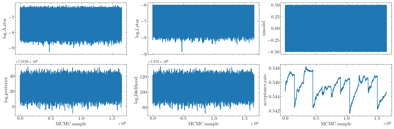
  Figure 2: Trace plots for the default settings of plot_chains for a model with two pulsar-common parameters, "log_A_star" and "log_f_star", and a merged chain of length $\sim 1.7\times 10^{6}$ after thinning and removal of the cut-off.

• plot_utils.plot_posteriors

  This function produces posterior plots from MCMC chains, see for example Figure 1. These plots are created using the GetDist package [17]. This package provides kernel density estimation of the marginalized 1D- and 2D-posterior densities obtained from MC sampling to produce smooth posterior plots. Note that for plot_posteriors, both the arguments chains and params are expected to be a list of chains and a list of parameter dictionaries, even if these lists contain only one item. You can superimpose the results of several runs by adding additional chains and parameter dictionaries to these lists. This is useful to compare a run set up with smbhb=True to a run without the SMBHB contribution. Several handy optional arguments for this function allow for user customization of the posterior plots. Here, we highlight the most useful features. For a more comprehensive list, please refer to the "Reference section" of PTArcade documentation web page.

  • As for plot_chains, you can specify the parameters to be plotted. This is done by passing a list of lists containing the desired parameter names for each model to par_to_plot. By default, all pulsar-common parameters are plotted.

  • You can adjust axis labels by passing a list of lists containing the desired formats for each parameter to par_to_plot. By default, the labels are the parameter names in params.

  • When analyzing a run with mod_sel=True, you can specify which hypermodel you want to plot using the model_id argument. It expects a list of zeros and ones, which select the desired hypermodel for each chain in chains. The default value is None, in which case hypermodel zero is plotted for every chain.

  • You can choose the confidence levels at which the highest posterior density intervals (HPI) are computed and shown in the 1D-posterior plots. The argument hpi_levels expects a list of floats between zero and one corresponding to the desired confidence levels. The default, hpi_levels=[0.68, 0.95], corresponds to 68% and 95% confidence levels. Note that confidence levels are specified for every chain in chains, not on a chain-by-chain basis.

  • You can choose the level at which to compute and plot the K-ratio bound using the k_ratio argument. This argument expects a list of float’s between zero and one corresponding to the desired K-ratio levels which were introduced in [12]. Each element in the list is associated with a chain in chains. The default value is None, in which case the K-ratio is not plotted. The K-ratio depends on the Bayes factor for the selected chain, and is, therefore, only sensible for PTArcade runs with model selection. For this feature to function properly, you need to pass a list of Bayes factors to the bf argument, where each element in bf was previously determined from the corresponding chain in chains. We keep the Bayes factors as an external input since computing the Bayes factor for a chain can be both time intensive and computationally expensive.

  • The 2D-posterior plots generated by plot_posteriors are shown as contour plots. You can adjust the confidence levels at which these contours are drawn using the levels argument. It expects a list of floats between zero and one, corresponding to the desired confidence level. The default value is None, in which case the contours correspond to 68% and 95% confidence level.

  • By setting the verbose argument to True, you can print a statistical summary for the chains in chains. This contains information on the confidence intervals, the K-ratio, the highest posterior density points, and the Bayes estimator for the 1D-marginalized posterior distributions of every parameter specified to plot_posteriors. The K-ratio and HPI intervals are determined based on the values passed to k_ratio and hpi_values.

4 Acknowledgments

We thank our colleagues in NANOGrav for fruitful discussions and feedback during the development of these tools. We particularly thank Luke Z. Kelley for helping derive the priors for the SMBHB signal, William Lamb for helping with the ceffyl implementation, and Rafael R. Lino dos Santos for helping debug PTArcade. This work was supported by the Deutsche Forschungsgemeinschaft under Germany’s Excellence Strategy - EXC 2121 Quantum Universe - 390833306.
Part of this work was conducted using the High Performance Computing Cluster PALMA II at the University of Münster (https://www.uni-muenster.de/IT/HPC). This work used the Maxwell computational resources operated at Deutsches Elektronen-Synchrotron DESY, Hamburg (Germany). This work was conducted in part using the HPC resources of the Texas Advanced Computing Center (TACC) at the University of Texas at Austin. The Tufts University High Performance Computing Cluster (https://it.tufts.edu/high-performance-computing) was utilized for some of the research reported in this paper. This research used the computational resources provided by the University of Central Florida’s Advanced Research Computing Center (ARCC).
The work of R.v.E., K.Sc., and T.S. is supported by the Deutsche Forschungsgemeinschaft (DFG) through the Research Training Group, GRK 2149: Strong and Weak Interactions – from Hadrons to Dark Matter. A.Mi. is supported by the Deutsche Forschungsgemeinschaft under Germany’s Excellence Strategy - EXC 2121 Quantum Universe - 390833306. K.D.O. was supported in part by NSF grants Nos. 2111738 and 2207267. T.T. contribution to this work is supported by the Fermi Research Alliance, LLC, under contract No. DE-AC02-07CH11359 with the U.S. Department of Energy, Office of Science, Office of High Energy Physics.

Attribute	Description
G	Newton’s constant ($\mathrm{GeV}^{-2}$)
	TYPE: np.float64
M_pl	Reduced Planck mass (GeV)
	TYPE: np.float64
T_0	Present-day temperature of the Universe ($\mathrm{GeV}$)
	TYPE: np.float64
z_eq	Redshift of matter-radiation equality
	TYPE: int
T_eq	Temperature of matter-radiation equality (GeV)
	TYPE: np.float64
h	Reduced Hubble parameter
	TYPE: float
H_0	Hubble constant (GeV)
	TYPE: np.float64
H_0_Hz	Hubble constant (Hz)
	TYPE: np.float64
omega_v	Present-day dark-energy density [43]
	TYPE: float
omega_m	Present-day matter density [43]
	TYPE: float
omega_r	Present-day radiation density [43]
	TYPE: float
A_s	Amplitude of the primordial scalar power-spectrum [43]
	TYPE: np.float64
f_cmb	CMB pivot-scale (Hz) [43]
	TYPE: float
gev_to_hz	Conversion from GeV to Hz
	TYPE: np.float64
g_rho_0	Present-day number of relativistic degrees of freedom
	TYPE: np.float64
g_rho_0	Present-day number of entropic relativistic degrees of freedom
	TYPE: np.float64

Table 2: Constants and conversion factors included in the models_utils module.

References

- Abbott et al. [2016] B. P. Abbott et al. (LIGO Scientific, Virgo), Phys. Rev. Lett. 116, 061102 (2016), arXiv:1602.03837 [gr-qc] .
- Maggiore [2000] M. Maggiore, Phys. Rept. 331, 283 (2000), arXiv:gr-qc/9909001 .
- Caprini and Figueroa [2018] C. Caprini and D. G. Figueroa, Class. Quant. Grav. 35, 163001 (2018), arXiv:1801.04268 [astro-ph.CO] .
- Christensen [2019] N. Christensen, Rept. Prog. Phys. 82, 016903 (2019), arXiv:1811.08797 [gr-qc] .
- Agazie et al. [2023a] G. Agazie et al. (NANOGrav), arXiv (2023a), submitted to arXiv.
- Rajagopal and Romani [1995] M. Rajagopal and R. W. Romani, ApJ 446, 543 (1995), arXiv:astro-ph/9412038 [astro-ph] .
- Jaffe and Backer [2003] A. H. Jaffe and D. C. Backer, Astrophys. J. 583, 616 (2003), arXiv:astro-ph/0210148 .
- Wyithe and Loeb [2003] J. S. B. Wyithe and A. Loeb, ApJ 590, 691 (2003), arXiv:astro-ph/0211556 [astro-ph] .
- Sesana et al. [2004] A. Sesana, F. Haardt, P. Madau, and M. Volonteri, Astrophys. J. 611, 623 (2004), arXiv:astro-ph/0401543 .
- Burke-Spolaor et al. [2019] S. Burke-Spolaor et al., Astron. Astrophys. Rev. 27, 5 (2019), arXiv:1811.08826 [astro-ph.HE] .
- Agazie et al. [2023b] G. Agazie et al. (NANOGrav), arXiv (2023b), in preparation.
- Afzal et al. [2023] A. Afzal et al. (NANOGrav), Astrophys. J. Lett. (2023), 10.3847/2041-8213/acdc91.
- Ellis et al. [2019] J. A. Ellis, M. Vallisneri, S. R. Taylor, and P. T. Baker, “ENTERPRISE: Enhanced Numerical Toolbox Enabling a Robust PulsaR Inference SuitE,” Astrophysics Source Code Library, record ascl:1912.015 (2019), ascl:1912.015 .
- Taylor et al. [2021] S. R. Taylor, P. T. Baker, J. S. Hazboun, J. Simon, and S. J. Vigeland, “enterprise_extensions,” (2021), v2.3.3.
- Lamb et al. [2023] W. G. Lamb, S. R. Taylor, and R. van Haasteren, “The need for speed: Rapid refitting techniques for bayesian spectral characterization of the gravitational wave background using ptas,” (2023), arXiv:2303.15442 [astro-ph.HE] .
- Foreman-Mackey [2016] D. Foreman-Mackey, The Journal of Open Source Software 1, 24 (2016).
- Lewis [2019] A. Lewis, (2019), arXiv:1910.13970 [astro-ph.IM] .
- McLaughlin [2013] M. A. McLaughlin, Class. Quant. Grav. 30, 224008 (2013), arXiv:1310.0758 [astro-ph.IM] .
- Hobbs et al. [2010] G. Hobbs et al., Classical and Quantum Gravity 27, 084013 (2010).
- Ramani et al. [2020] H. Ramani, T. Trickle, and K. M. Zurek, JCAP 12, 033 (2020), arXiv:2005.03030 [astro-ph.CO] .
- Lee et al. [2021a] V. S. H. Lee, A. Mitridate, T. Trickle, and K. M. Zurek, JHEP 06, 028 (2021a), arXiv:2012.09857 [astro-ph.CO] .
- Lee et al. [2021b] V. S. H. Lee, S. R. Taylor, T. Trickle, and K. M. Zurek, JCAP 08, 025 (2021b), arXiv:2104.05717 [astro-ph.CO] .
- Vallisneri et al. [2020] M. Vallisneri et al. (NANOGrav), ApJ (2020), 10.3847/1538-4357/ab7b67, arXiv:2001.00595 [astro-ph.HE] .
- Arzoumanian et al. [2016] Z. Arzoumanian et al. (NANOGrav), Astrophys. J. 821, 13 (2016), arXiv:1508.03024 [astro-ph.GA] .
- Arzoumanian et al. [2018] Z. Arzoumanian et al. (NANOGRAV), Astrophys. J. 859, 47 (2018), arXiv:1801.02617 [astro-ph.HE] .
- Alam et al. [2021] M. F. Alam et al. (NANOGrav), Astrophys. J. Suppl. 252, 4 (2021), arXiv:2005.06490 [astro-ph.HE] .
- Arzoumanian et al. [2020] Z. Arzoumanian et al., Astrophys. J. Lett. 905, L34 (2020).
- Agazie et al. [2023c] G. Agazie et al. (NANOGrav), arXiv (2023c), submitted to arXiv.
- Antoniadis et al. [2022] J. Antoniadis et al., Mon. Not. Roy. Astron. Soc. 510, 4873 (2022), arXiv:2201.03980 [astro-ph.HE] .
- Hellings and Downs [1983] R. W. Hellings and G. S. Downs, Astrophys. J. Lett. 265, L39 (1983).
- Allen and Romano [1999] B. Allen and J. D. Romano, Phys. Rev. D 59, 102001 (1999), arXiv:gr-qc/9710117 .
- Phinney [2001] E. S. Phinney, arXiv e-prints , astro-ph/0108028 (2001), arXiv:astro-ph/0108028 [astro-ph] .
- van Haasteren and Levin [2012] R. van Haasteren and Y. Levin, Monthly Notices of the Royal Astronomical Society 428, 1147 (2012).
- Lentati et al. [2013] L. Lentati, P. Alexander, M. P. Hobson, S. Taylor, J. Gair, S. T. Balan, and R. van Haasteren, Physical Review D 87 (2013), 10.1103/physrevd.87.104021.
- Agazie et al. [2023d] G. Agazie et al. (NANOGrav), Astrophys. J. Lett. (2023d), 10.3847/2041-8213/acda9a.
- Ellis and van Haasteren [2017] J. Ellis and R. van Haasteren, “jellis18/ptmcmcsampler: Official release,” (2017).
- Carlin and Chib [1995] B. P. Carlin and S. Chib, Journal of the Royal Statistical Society. Series B (Methodological) 57, 473 (1995).
- Godsill [2001] S. J. Godsill, Journal of Computational and Graphical Statistics 10, 230 (2001).
- Hee et al. [2015] S. Hee, W. J. Handley, M. P. Hobson, and A. N. Lasenby, Monthly Notices of the Royal Astronomical Society 455, 2461 (2015), https://academic.oup.com/mnras/article-pdf/455/3/2461/9377568/stv2217.pdf .
- Efron and Tibshirani [1986] B. Efron and R. Tibshirani, Statist. Sci. 57, 54 (1986).
- Zyla et al. [2020] P. A. Zyla et al. (Particle Data Group), PTEP 2020, 083C01 (2020).
- Saikawa and Shirai [2020] K. Saikawa and S. Shirai, Journal of Cosmology and Astroparticle Physics 2020, 011 (2020).
- Aghanim et al. [2020] N. Aghanim et al. (Planck), Astron. Astrophys. 641, A6 (2020), [Erratum: Astron.Astrophys. 652, C4 (2021)], arXiv:1807.06209 [astro-ph.CO] .