Modeling realistic multiphase flows using a non-orthogonal multiple-relaxation-time lattice Boltzmann method

Abstract

In this paper, we develop a three-dimensional multiple-relaxation-time lattice Boltzmann method (MRT-LBM) based on a set of non-orthogonal basis vectors. Compared with the classical MRT-LBM based on a set of orthogonal basis vectors, the present non-orthogonal MRT-LBM simplifies the transformation between the discrete velocity space and the moment space, and exhibits better portability across different lattices. The proposed method is then extended to multiphase flows at large density ratio with tunable surface tension, and its numerical stability and accuracy are well demonstrated by some benchmark cases. Using the proposed method, a practical case of a fuel droplet impacting on a dry surface at high Reynolds and Weber numbers is simulated and the evolution of the spreading film diameter agrees well with the experimental data. Furthermore, another realistic case of a droplet impacting on a super-hydrophobic wall with a cylindrical obstacle is reproduced, which confirms the experimental finding of Liu et al. [“Symmetry breaking in drop bouncing on curved surfaces,” Nature communications 6, 10034 (2015)] that the contact time is minimized when the cylinder radius is comparable with the droplet cylinder.

I Introduction

Interfaces between different phases and/or components are ubiquitous in multiphase flows and energy applications, such as rain dynamics, plant spraying, water boiling, gas turbine blade cooling, to name but a few Richard, Clanet, and Quéré (2002); Li et al. (2016). A deeper understanding of the fundamental physics of such complex interfaces is of great importance in many natural and industrial processes. The dynamics of the interfaces is difficult to investigate because typical interfaces are extremely thin, complex in shape and deforming at short time scales. In addition, the density ratio, Weber and Reynolds numbers involved in many practical multiphase flows, such as binary droplets collisions and melt-jet breakup, are usually very high, which further increases the complexity of the phenomena involved. Therefore, development of robust and accurate computational methods to capture the complex interfacial phenomena is crucial in the study of multiphase flows.

During the last three decades, the mesoscopic lattice Boltzmann method (LBM), based on the kinetic theory, has become an increasingly important method for numerical simulations of multiphase flows, mainly on account of its meso-scale features, easy implementation and computational efficiency Shan and Chen (1993); Yuan and Schaefer (2006); Gan et al. (2011); Li et al. (2012); Lycett-Brown et al. (2014); Monaco, Brenner, and Luo (2014); Succi (2015); Li et al. (2015); Lycett-Brown and Luo (2015, 2016); Mazloomi Moqaddam, Chikatamarla, and Karlin (2016); Fu et al. (2017); Saito, Abe, and Koyama (2017); Saito et al. (2018); Qin et al. (2018); Cui, Wang, and Liu (2019); Chen et al. (2019). Generally, the existing multiphase LB models can be classified into four categories: the color-gradient model Gunstensen et al. (1991); Grunau, Chen, and Eggert (1993), the pseudopotential model Shan and Chen (1993, 1994), the free-energy model Swift, Osborn, and Yeomans (1995); Swift et al. (1996) and the mean-field model He, Chen, and Zhang (1999). Among them, the pseudopotential model is considered in the present work due to its simplicity and computational efficiency. In this model, the interactions among populations of molecules are modeled by a density-dependent pseudopotential. Through interactions among the particles on the nearest-neighboring sites, phase separation and breakup and/or merging of phase interfaces can be achieved automatically. For further details about the multiphase LB models, interested readers are directed to some comprehensive review papers Li et al. (2016); Chen et al. (2014); Liu et al. (2016a).

In the LBM framework, the fluid is usually represented by populations of fictitious particles colliding locally and streaming to adjacent nodes along the links of a regular lattice. The macroscopic variables are obtained through a set of rules based on the calculated particle distribution functions (DFs). In particular, the simplest scheme to execute the “colliding” (or collision) step is to relax all the distribution functions (DFs) to their local equilibria at an identical rate, known as the single-relaxation-time (SRT) scheme Qian, d’Humières, and Lallemand (1992). However, SRT-LBM usually suffers numerical instability for flows with even moderate Reynolds number. Compared with SRT scheme, the multi-relaxation-time (MRT) scheme, originally formulated in Higuera, Succi, and Benzi (1989); d’Humieres (1994) and later extended in Lallemand and Luo (2000); d’Humières (2002), is able to enhance the stability by carefully separating the time scales among the kinetic modes. To enhance numerical stability of LBM, some modified approaches within the SRT framework have also been proposed, such as the entropic LBM Karlin, Ferrante, and Öttinger (1999); Ansumali and Karlin (2000) and regularized LBM Zhang, Shan, and Chen (2006); Latt and Chopard (2006). In addition, the cascaded lattice Boltzmann method (CLBM), which employs moments in a co-moving frame in contrast to the stationary moments in MRT, has also been shown to improve numerical stability significantly compared with the classical SRT-LBM Geier, Greiner, and Korvink (2006); Lycett-Brown et al. (2014); Lycett-Brown and Luo (2016); De Rosis (2017); Fei et al. (2018a); Saito et al. (2018).

The present work focuses on the MRT-LBM, in which the collision step is carried out in a (raw) moment space via a transformation matrix ${\bf{M}}$, where different moments can be relaxed independently. The post-collision moments are then transformed back via ${{\bf{M}}^{{\rm{-}}1}}$ and the streaming step is implemented in the discrete velocity space as usual. Usually, the Gram-Schmidt procedure is adopted to construct an orthogonal transformation matrix Lallemand and Luo (2000); d’Humières (2002); Suga et al. (2015); Saito, Abe, and Koyama (2017), which means that the basis vectors for the moments are orthogonal to one another. It is known that the widely used orthogonal MRT-LBM is more complex and computationally expensive than SRT-LBM, especially for three-dimensional problems. To the best of our knowledge, orthogonality is not a necessary condition for stability. As an early attempt, Lycett-Brown and Luo Lycett-Brown and Luo (2014) showed that an MRT-LBM based on a non-orthogonal basis vector set enhances the numerical stability compared with the SRT-LBM. The corresponding non-orthogonal MRT-LBM has been extended to simulate incompressible thermal flows by Liu et al. Liu et al. (2016b). In addition, it was shown by Li et al. Li et al. (2018) that a non-orthogonal MRT-LBM can retain the numerical accuracy while simplifying the implementation of its orthogonal counterpart. In parallel, the CLBM Geier, Greiner, and Korvink (2006), which can be viewed as a non-orthogonal MRT-LBM in the co-moving frame, has been shown to possess very good numerical stability for high Rayleigh number thermal flows Fei, Luo, and Li (2018), as well as high Reynolds and Weber numbers multiphase flows Lycett-Brown et al. (2014); Saito et al. (2018); Lycett-Brown and Luo (2016). Recently, an improved three-dimensional (3D) CLBM has been proposed by Fei et al. Fei et al. (2018a), where an improved set of non-orthogonal basis vectors was employed and a generalized multiple-relaxation-time (GMRT) scheme Fei et al. (2018a); Fei and Luo (2017) was adopted to cast MRT-LBM and CLBM into a unified framework. Within the GRMT framework, the CLBM can reduce to a non-orthogonal MRT-LBM when the shift matrix is a unit matrix, where the shift matrix is defined to shift (raw) moments of the DFs to the corresponding central moments.

In this work, we first give a theoretical analysis to construct a generalized non-orthogonal MRT-LBM based on the basis vector set proposed in Ref. Fei, Luo, and Li (2018). Coupled with the pseudopotential multiphase model, the proposed non-orthogonal MRT-LBM is extended to simulate multiphase flows with large density ratio and tunable surface tension, which is then verified by some benchmark cases. Finally, we provide simulations of two practical and challenging problems using our proposed non-orthogonal MRT-LBM, to highlight its capability for simulating realistic multiphase flows.

II Non-orthogonal MRT-LBM for multiphase flows

The theoretical derivation of the non-orthogonal MRT-LBM is given in this section. Firstly, the MRT framework is introduced briefly. Then, the choice of the non-orthogonal basis vector set is presented. In the end, the pseudopotential model is incorporated into the present method to simulate multiphase flows.

II.1 MRT framework

In this section, the MRT-LBM framework is introduced based on the standard D3Q27 discrete velocity model (DVM). However, it should be noted that the procedures shown in this work are not limited to the specified DVM, and can be extended to other DVMs readily. The lattice speed $c=\Delta x=\Delta t=1$ and the lattice sound speed ${c_{s}}=1/\sqrt{3}$ are adopted, in which $\Delta x$ and $\Delta t$ are the lattice spacing and time step, respectively. The discrete velocities ${{\bf{e}}_{i}}=[\left|{{e_{ix}}}\right\rangle,\left|{{e_{iy}}}\right\rangle,\left|{{e_{iz}}}\right\rangle]$ are defined as

$$\begin{array}[]{l}\left|{{e_{ix}}}\right\rangle={[0,1,-1,0,0,0,0,1,-1,1,-1,1,-1,1,-1,0,0,0,0,1,-1,1,-1,1,-1,1,-1]^{\top}},\\ \left|{{e_{iy}}}\right\rangle={[0,0,0,1,-1,0,0,1,1,-1,-1,0,0,0,0,1,-1,1,-1,1,1,-1,-1,1,1,-1,-1]^{\top}},\\ \left|{{e_{i{\rm{z}}}}}\right\rangle={[0,0,0,0,0,1,-1,0,0,0,0,1,1,-1,-1,1,1,-1,-1,1,1,1,1,-1,-1,-1,-1]^{\top}}.\\ \end{array}$$ (1)

where $i=0,1,...,26$, ${\left|\cdot\right\rangle}$ denotes a 27-dimensional column vector, and the superscript $\top$ denotes the transposition.

To execute the collision step in the moment space, we first define moments of the discrete distribution function (DFs) ${f_{i}}$,

$${k_{mnp}}=\left\langle{{f_{i}}|e_{ix}^{m}e_{iy}^{n}e_{iz}^{p}}\right\rangle,$$ (2)

where $m$, $n$, and $p$ are integers. The equilibrium moments $k_{mnp}^{eq}$ are defined analogously by replacing ${f_{i}}$ with the discrete equilibrium distribution functions (EDFs) $f_{i}^{eq}$. To construct an MRT-LBM, an appropriate moment set vector ${\bf{m}}$ is needed,

$${\bf{m}}={[{m_{0}},{m_{1}},...,{m_{26}}]^{\rm T}}$$ (3)

where the elements in ${\bf{m}}$ are combinations of ${k_{mnp}}$. The transformation from the discrete velocity space to the moment space can be performed through a transformation matrix ${\bf{M}}$ by ${\bf{m}}={\bf{Mf}}$. The explicit expression for ${\bf{M}}$ depends on the raw moment set in Eq. (3) , which will be discussed in the next subsection.

A general collision step in MRT-LBM can be written as Li et al. (2010),

$$f_{i}^{*}({\bf{x}},t)={f_{i}}({\bf{x}},t)-{\Lambda_{i,k}}[{f_{k}}-f_{k}^{eq}]{|_{({\bf{x}},t)}}+\frac{{\Delta t}}{2}[{\bar{F}_{i}}({\bf{x}},t)+{\bar{F}_{i}}({\bf{x}}+{{\bf{e}}_{i}}\Delta t,t+\Delta t)],$$ (4)

where ${\bf{x}}$ is the spatial position, $t$ is time, ${\bar{F}_{i}}$ are the forcing terms in the discrete velocity space, and ${\Lambda_{i,k}}={({{\bf{M}}^{{\bf{-1}}}}{\bf{SM}})_{i,k}}$ is the collision operator, in which ${\bf{S}}$ is a diagonal relaxation matrix. The EDFs $f_{i}^{eq}$ are often given by a low-Mach truncation form,

$$f_{i}^{eq}=\rho\omega({\left|{{{\bf{e}}_{i}}}\right|^{2}})\left[{1+\frac{{{{\bf{e}}_{i}}\cdot{\bf{u}}}}{{c_{s}^{2}}}+\frac{{{\bf{uu}}:({{\bf{e}}_{i}}{{\bf{e}}_{i}}-c_{s}^{2})}}{{c_{s}^{4}}}}\right]$$ (5)

where $\rho$ is the fluid density, ${\bf{u}}=[{u_{x}},{u_{y}},{u_{z}}]$ is the fluid velocity, and the weights are $\omega(0)=8/27$, $\omega(1)=2/27$, $\omega(2)=1/54$ and $\omega(3)=1/216$. According to the analysis by Guo et al. Guo, Zheng, and Shi (2002), the forcing terms are defined as,

$${{\bar{F}}_{i}}{\rm{=}}\omega({\left|{{{\bf{e}}_{i}}}\right|^{2}})\left[{\frac{{{{\bf{e}}_{i}}-{\bf{u}}}}{{c_{s}^{2}}}+\frac{{({\bf{u}}\cdot{{\bf{e}}_{i}}){{\bf{e}}_{i}}}}{{c_{s}^{4}}}}\right]\cdot{\bf{F}},$$ (6)

where ${\bf{F}}=[{F_{x}},{F_{y}},{F_{z}}]$ is the total force exerted on the fluid system.

To remove the implicit implementation, Eq. (4) can be modified as,

$${\bar{f}_{i}}({\bf{x}}+{{\bf{e}}_{i}}\Delta t,t+\Delta t)={\bar{f}_{i}}({\bf{x}},t)-{\Lambda_{i,k}}[{\bar{f}_{k}}-f_{k}^{eq}]{|_{({\bf{x}},t)}}+({\bf{I}}-\frac{{{\Lambda_{i,k}}}}{2}){\bar{F}_{i}}({\bf{x}},t)\Delta t,$$ (7)

where ${\bar{f}_{i}}={f_{i}}-\Delta t{\bar{F}_{i}}/2$ and ${\bf{I}}$ is the unit matrix. Multiplying Eq. (7) by the transformation matrix ${\bf{M}}$, the collision step in the moment space can be rewritten as

$${{\bf{\bar{m}}}^{*}}={\bf{\bar{m}}}-{\bf{S}}({\bf{\bar{m}}}-{{\bf{\bar{m}}}^{eq}})+({\bf{I}}-\frac{{\bf{S}}}{2})\Delta t{\bf{\tilde{F}}},$$ (8)

where ${\bf{\bar{m}}}={\bf{M\bar{f}}}$, ${{\bf{m}}^{eq}}={\bf{M}}{{\bf{f}}^{eq}}$ and ${\bf{\tilde{F}}}={\bf{M\bar{F}}}$.

After the collision step, post-collision discrete DFs can be reconstructed by ${{\bf{\bar{f}}}^{\rm{*}}}={{\bf{M}}^{-1}}{{\bf{\bar{m}}}^{*}}$. In the streaming step, the post-collision discrete DFs in space ${\bf{x}}$ stream to their neighbors $({\bf{x}}+{{\bf{e}}_{i}}\Delta t)$ along the characteristic lines as usual,

$${\bar{f}_{i}}({\bf{x}}+{{\bf{e}}_{i}}\Delta t,t+\Delta t)=\bar{f}_{i}^{*}({\bf{x}},t)$$ (9)

The hydrodynamic variables are updated by

$$\rho=\sum\limits_{i}{{{\bar{f}}_{i}},}~{}~{}~{}{\rm{}}\rho{\bf{u}}=\sum\limits_{i}{{{\bar{f}}_{i}}}{{\bf{e}}_{i}}+\frac{{\Delta t{\bf{F}}}}{2}.$$ (10)

II.2 Non-orthogonal basis vector set

In this work, we adopt a moment set ${\bf{m}}={[{m_{0}},{m_{1}},...,{m_{26}}]^{\rm T}}$ with the following 27 moment elements (in the ascending order of $m+n+p$ ),

$$\begin{array}[]{l}{\bf{m}}=[{k_{000}},{k_{100}},{k_{010}},{k_{001}},{k_{110}},{k_{101}},{k_{011}},{k_{200}}+{k_{020}}+{k_{002}},{k_{200}}-{k_{020}},{k_{200}}-{k_{002}},{k_{120}},\\ {\rm{}}{k_{102}},{k_{210}},{k_{201}},{k_{012}},{k_{021}},{k_{111}},{k_{220}},{k_{202}},{k_{022}},{k_{211}},{k_{121}},{k_{112}},{k_{122}},{k_{212}},{k_{221}},{k_{222}}{]^{\rm T}}\\ \end{array}$$ (11)

where the elements ${m_{0}}$ , ${m_{1-3}}$, and ${m_{4-9}}$ are related to the fluid density, momentum, and viscous stress tensor, respectively, while the remaining elements are higher-order moments which do not affect the consistency at the Navier-Stokes level. It should be pointed out that the moments are chosen based on two criteria: (i) the basis vectors for the moments are linearly independent (but not necessarily orthogonal to one another); (ii) the calculation of each moment is as simple as possible. Generally, the high-order elements are related to some kinetic moments, such as energy flux and square of kinetic energy, but the relations are not defined exactly. The above moment set in Eq. (11) was originally adopted in our cascaded LBM to improve the implementation Fei, Luo, and Li (2018), where the mixed second-order moments $({k_{200}}+{k_{020}}+{k_{002}},{k_{200}}-{k_{020}},{k_{200}}-{k_{002}})$ were implicit and the relaxation matrix was slightly modified to simplify the map between the (raw) moment space and central moment space. In the present paper, the relaxation matrix ${\bf{S}}$ is a diagonal matrix,

$${\bf{S}}=diag({s_{0}},{s_{1}},{s_{1}},{s_{1}},{s_{2}},{s_{2}},{s_{2}},{s_{2b}},{s_{2}},{s_{2}},{s_{3}},{s_{3}},{s_{3}},{s_{3}},{s_{3}},{s_{3}},{s_{3b}},{s_{4}},{s_{4}},{s_{4}},{s_{4b}},{s_{4b}},{s_{4b}},{s_{5}},{s_{5}},{s_{5}},{s_{6}}),$$ (12)

where the elements are the relaxation rates for different moments. The kinematic and bulk viscosities are related to the relaxation rates for the second-order moments by $\nu=(1/{s_{2}}-0.5)c_{s}^{2}\Delta t$ and $\xi=2/3(1/{s_{2b}}-0.5)c_{s}^{2}\Delta t$, respectively. Here, we use ${s_{0}}={s_{1}}=1.0$, ${s_{2b}}={s_{3b}}=0.6$ and the others are set to be 1.2.

The transformation matrix ${\bf{M}}$ can be obtained explicitly according to Eq. (2) and Eq. (11),

$${\bf{M}=}\left[\begin{array}[]{l r r r r r r r r r r r r r r r r r r r r r r r r r r}1&1&1&1&1&1&1&1&1&1&1&1&1&1&1&1&1&1&1&1&1&1&1&1&1&1&1\\ 0&1&-1&0&0&0&0&1&-1&1&-1&1&-1&1&-1&0&0&0&0&1&-1&1&-1&1&-1&1&-1\\ 0&0&0&1&-1&0&0&1&1&-1&-1&0&0&0&0&1&-1&1&-1&1&1&-1&-1&1&1&-1&-1\\ 0&0&0&0&0&1&-1&0&0&0&0&1&1&-1&-1&1&1&-1&-1&1&1&1&1&-1&-1&-1&-1\\ 0&0&0&0&0&0&0&1&-1&-1&1&0&0&0&0&0&0&0&0&1&-1&-1&1&1&-1&-1&1\\ 0&0&0&0&0&0&0&0&0&0&0&1&-1&-1&1&0&0&0&0&1&-1&1&-1&-1&1&-1&1\\ 0&0&0&0&0&0&0&0&0&0&0&0&0&0&0&1&-1&-1&1&1&1&-1&-1&-1&-1&1&1\\ 0&1&1&1&1&1&1&2&2&2&2&2&2&2&2&2&2&2&2&3&3&3&3&3&3&3&3\\ 0&1&1&-1&-1&0&0&0&0&0&0&1&1&1&1&-1&-1&-1&-1&0&0&0&0&0&0&0&0\\ 0&1&1&0&0&-1&-1&1&1&1&1&0&0&0&0&-1&-1&-1&-1&0&0&0&0&0&0&0&0\\ 0&0&0&0&0&0&0&1&-1&1&-1&0&0&0&0&0&0&0&0&1&-1&1&-1&1&-1&1&-1\\ 0&0&0&0&0&0&0&0&0&0&0&1&-1&1&-1&0&0&0&0&1&-1&1&-1&1&-1&1&-1\\ 0&0&0&0&0&0&0&1&1&-1&-1&0&0&0&0&0&0&0&0&1&1&-1&-1&1&1&-1&-1\\ 0&0&0&0&0&0&0&0&0&0&0&1&1&-1&-1&0&0&0&0&1&1&1&1&-1&-1&-1&-1\\ 0&0&0&0&0&0&0&0&0&0&0&0&0&0&0&1&-1&1&-1&1&1&-1&-1&1&1&-1&-1\\ 0&0&0&0&0&0&0&0&0&0&0&0&0&0&0&1&1&-1&-1&1&1&1&1&-1&-1&-1&-1\\ 0&0&0&0&0&0&0&0&0&0&0&0&0&0&0&0&0&0&0&1&-1&-1&1&-1&1&1&-1\\ 0&0&0&0&0&0&0&1&1&1&1&0&0&0&0&0&0&0&0&1&1&1&1&1&1&1&1\\ 0&0&0&0&0&0&0&0&0&0&0&1&1&1&1&0&0&0&0&1&1&1&1&1&1&1&1\\ 0&0&0&0&0&0&0&0&0&0&0&0&0&0&0&1&1&1&1&1&1&1&1&1&1&1&1\\ 0&0&0&0&0&0&0&0&0&0&0&0&0&0&0&0&0&0&0&1&1&-1&-1&-1&-1&1&1\\ 0&0&0&0&0&0&0&0&0&0&0&0&0&0&0&0&0&0&0&1&-1&1&-1&-1&1&-1&1\\ 0&0&0&0&0&0&0&0&0&0&0&0&0&0&0&0&0&0&0&1&-1&-1&1&1&-1&-1&1\\ 0&0&0&0&0&0&0&0&0&0&0&0&0&0&0&0&0&0&0&1&-1&1&-1&1&-1&1&-1\\ 0&0&0&0&0&0&0&0&0&0&0&0&0&0&0&0&0&0&0&1&1&-1&-1&1&1&-1&-1\\ 0&0&0&0&0&0&0&0&0&0&0&0&0&0&0&0&0&0&0&1&1&1&1&-1&-1&-1&-1\\ 0&0&0&0&0&0&0&0&0&0&0&0&0&0&0&0&0&0&0&1&1&1&1&1&1&1&1\\ \end{array}\right].$$ (13)

The equilibrium raw moment vector ${{\bf{m}}^{eq}}=[m_{0}^{eq},m_{1}^{eq},...,m_{26}^{eq}]$ finally reads

$$\begin{array}[]{l}{{\bf{m}}^{eq}}=[\rho,\rho{u_{x}},\rho{u_{y}},\rho{u_{z}},\rho{u_{x}}{u_{y}},\rho{u_{x}}{u_{z}},\rho{u_{y}}{u_{z}},\rho(1+{{\bf{u}}^{2}}),\rho(u_{x}^{2}-u_{y}^{2}),\rho(u_{x}^{2}-u_{z}^{2}),\\ \rho c_{s}^{2}{u_{x}},\rho c_{s}^{2}{u_{x}},\rho c_{s}^{2}{u_{y}},\rho c_{s}^{2}{u_{z}},\rho c_{s}^{2}{u_{y}},\rho c_{s}^{2}{u_{z}},0,\rho c_{s}^{2}(c_{s}^{2}+u_{x}^{2}+u_{y}^{2}),\rho c_{s}^{2}(c_{s}^{2}+u_{x}^{2}+u_{z}^{2}),\\ \rho c_{s}^{2}(c_{s}^{2}+u_{y}^{2}+u_{z}^{2}),\rho c_{s}^{2}{u_{y}}{u_{z}},\rho c_{s}^{2}{u_{x}}{u_{z}},\rho c_{s}^{2}{u_{x}}{u_{y}},\rho c_{s}^{4}{u_{x}},\rho c_{s}^{4}{u_{y}},\rho c_{s}^{4}{u_{z}},\rho c_{s}^{4}{{\bf{u}}^{2}}+\rho c_{s}^{6}{]^{\rm T}}\\ \end{array}$$ (14)

and the forcing term vector in the moment space ${\bf{\tilde{F}}}=[{\tilde{F}_{0}},{\tilde{F}_{1}},...,{\tilde{F}_{26}}]$,

$$\begin{array}[]{l}{\bf{\tilde{F}}}=[0,{F_{x}},{F_{y}},{F_{z}},{F_{x}}{u_{y}}+{F_{y}}{u_{x}},{F_{x}}{u_{z}}+{F_{z}}{u_{x}},{F_{y}}{u_{z}}+{F_{z}}{u_{y}},2{\bf{F}}\cdot{\bf{u}},2({F_{x}}{u_{x}}-{F_{y}}{u_{y}}),2({F_{x}}{u_{x}}-{F_{\rm{z}}}{u_{z}}),\\ {F_{x}}c_{s}^{2},{F_{x}}c_{s}^{2},{F_{y}}c_{s}^{2},{F_{z}}c_{s}^{2},{F_{y}}c_{s}^{2},{F_{z}}c_{s}^{2},0,2c_{s}^{2}({F_{x}}{u_{x}}+{F_{y}}{u_{y}}),2c_{s}^{2}({F_{x}}{u_{x}}+{F_{z}}{u_{z}}),2c_{s}^{2}({F_{y}}{u_{y}}+{F_{z}}{u_{z}}),\\ c_{s}^{2}({F_{y}}{u_{z}}+{F_{z}}{u_{y}}),c_{s}^{2}({F_{x}}{u_{z}}+{F_{z}}{u_{x}}),c_{s}^{2}({F_{x}}{u_{y}}+{F_{y}}{u_{x}}),c_{s}^{4}{F_{x}},c_{s}^{4}{F_{y}},c_{s}^{4}{F_{z}},2c_{s}^{4}{\bf{F}}\cdot{\bf{u}}{]^{\rm T}}\\ \end{array}$$ (15)

It can be found that the transformation matrix ${\bf{M}}$ in Eq. (13) is non-orthogonal. Through the Chapman-Enskog analysis (see Appendix A), the proposed non-orthogonal MRT-LBM can recover the Navier-Stokes equations in the low Mach number limit. When all the relaxation parameters in the matrix ${\bf{S}}$ are set equal, the present non-orthogonal MRT-LBM reduces to the SRT-LBM. Compared with the orthogonal MRT-LBM used in d’Humières (2002); Suga et al. (2015), the numbers of non-zeros in the present non-orthogonal ${\bf{M}}$ and its inverse matrix ${{\bf{M}}^{-1}}$ are much smaller (see in Table 1), which indicates the implementation is simplified and the computational efficiency is enhanced. Quantitatively, the non-orthogonal MRT-LBM requires approximately 25% and 15% less computational time for the D3Q27 model and D3Q19 model Fei, Luo, and Li (2018); Li et al. (2018), respectively. Moreover, a non-orthogonal D3Q19 MRT-LBM can be extracted from the D3Q27 model directly (see Appendix C, all the elements in ${\bf{m}}$, ${{\bf{m}}^{eq}}$, ${\bf{s}}$, ${\bf{\tilde{F}}}$, ${\bf{M}}$, and ${{\bf{M}}^{-1}}$ for the D3Q19 model can be extracted from the D3Q27 model directly), which means that the non-orthogonal MRT-LBM exhibits very good portability across lattices. The comparison between the non-orthogonal and orthogonal MRT-LBMs on the D3Q19 lattice is also shown in Table 1. Interested readers are kindly directed to the Supplementary Material for the explicit expressions of ${\bf{M}}$ and ${{\bf{M}}^{-1}}$.

Table 1: Non-zero numbers in ${\bf{M}}$ and ${{\bf{M}}^{{\rm{-}}1}}$ for orthogonal and non-orthognal MRT models.

	Orthogonal d’Humières (2002); Suga et al. (2015)		Non-orthogonal
Models	D3Q27	D3Q19	D3Q27	D3Q19
${\bf{M}}$	416	213	339	139
${{\bf{M}}^{{\rm{-}}1}}$	416	213	226	101

II.3 Multiphase model

To extend the above mentioned non-orthogonal MRT-LBM to multiphase flows, the pseudopotential model Shan and Chen (1993, 1994) is considered in the present work. It may be noted that the present non-orthogonal MRT-LBM can be also coupled with other multiphase models in a similar way. In the pseudopotential model, the interactions among molecules clusters are modeled by a pseudo-interaction force among fictitious particles,

$${{\bf{F}}_{{\rm{int}}}}=-G\psi({\bf{x}})\sum\limits_{i}{w({{\left|{{{\bf{e}}_{i}}}\right|}^{2}})}\psi({\bf{x}}+{{\bf{e}}_{i}}\Delta t){{\bf{e}}_{i}}$$ (16)

where G is the interaction strength, $\psi$ is a density-dependent pseudopotential, and the normalized weights are $w({\left|{{{\bf{e}}_{i}}}\right|^{2}})=\omega({\left|{{{\bf{e}}_{i}}}\right|^{2}})/c_{s}^{2}$ . According to the Chapman-Enskog analysis, the bulk pressure reads,

$$p=\rho c_{s}^{2}+\frac{{G{c^{2}}}}{2}{\psi^{2}}$$ (17)

In order to incorporate different equations of state consistently and achieve large density ratio, the square-root-form pseudopotential Yuan and Schaefer (2006) $\psi=\sqrt{2({p_{EOS}}-\rho c_{s}^{2})/G{c^{2}}}$ is used in this work, where ${p_{EOS}}$ is given by the adopted equation of state. Furthermore, some terms in ${\bf{\tilde{F}}}$ need to be slightly modified for the sake of thermodynamic consistency and tunable surface tension Li et al. (2012); Li, Luo, and Li (2013); Li and Luo (2013), and the details are provided in Appendix B.

III Numerical verification

III.1 Realization of large density ratio

First, we consider the verification of the liquid and vapor coexistence densities at large density ratios. To achieve large density ratios, different equations of state can be incorporated into the pseudopotential model, such as the Carnahan-Starling (C-S) equation, Peng-Robinson (P-R) equation and the piecewise linear equation of state Li, Luo, and Li (2013); Xu et al. (2015); Gong, Chen, and Yan (2017); Colosqui et al. (2012). In this paper, we use the piecewise equation of state, which is given by Colosqui et al. (2012),

$$p(\rho)=\left\{\begin{array}[]{l}\rho{\theta_{v}},~{}~{}{\rm{}}\rho\leq{\rho_{1}}\\ {\rho_{1}}{\theta_{v}}+(\rho-{\rho_{1}}){\theta_{m}},~{}~{}{\rm{}}{\rho_{1}}\leq\rho\leq{\rho_{2}}\\ {\rho_{1}}{\theta_{v}}+({\rho_{2}}-{\rho_{1}}){\theta_{m}}+(\rho-{\rho_{2}}){\theta_{l}},~{}~{}{\rm{}}\rho>{\rho_{2}}\\ \end{array}\right.$$ (18)

where ${\theta_{v}}={(\partial p/\partial\rho)_{v}}>0$ , ${\theta_{l}}={(\partial p/\partial\rho)_{l}}>0$ , and ${\theta_{m}}={(\partial p/\partial\rho)_{m}}<0$ are the slopes of $p(\rho)$ in the vapor-phase region, the liquid-phase region and the mechanically unstable region, respectively. In addition, $\sqrt{{\theta_{v}}}$ and $\sqrt{{\theta_{l}}}$ can be regarded as the sound speed in the vapor and liquid phases, respectively. The unknown ${\rho_{1}}$ and ${\rho_{2}}$, defining the spinodal points are obtained by solving the following two equations, which is related to the mechanical and chemical equilibrium conditions,

$$\begin{array}[]{l}\int_{{\rho_{v}}}^{{\rho_{l}}}{({\rho_{1}}-{\rho_{v}}){\theta_{v}}+({\rho_{2}}-{\rho_{1}})}{\theta_{m}}+({\rho_{l}}-{\rho_{2}}){\theta_{l}}=0,\\ \int_{{\rho_{v}}}^{{\rho_{l}}}{\frac{1}{\rho}dp=\log(}{\rho_{1}}/{\rho_{v}}){\theta_{v}}+\log({\rho_{2}}/{\rho_{1}}){\theta_{m}}+\log({\rho_{l}}/{\rho_{2}}){\theta_{l}}=0.\\ \end{array}$$ (19)

where ${\rho_{v}}$ and ${\rho_{l}}$ are vapor and liquid coexistence densities, respectively. It is known that the equilibrium coexistence densities are completely determined by the mechanical stability condition for flat interfaces. However, for circular interfaces (e.g., droplets, bubbles), the Laplace’s law also affects the coexistence densities. Due to the relatively large surface tension in the pseudopotential model (compared with the case in nature), the coexistence densities, especially the vapor phase density ${\rho_{v}}$, usually change with the radius of curvature, and this density deviation is more significant for the large density ratio problems. For example, the vapor-density deviation can be as large as 60 $\%$ for a system with ${\rho_{l}}/{\rho_{v}}{\rm{=}}100$ Li and Luo (2014). Li et al. proposed that the density deviation can be much reduced by setting the vapor-phase sound speed $\sqrt{{\theta_{v}}}$ to be the same the magnitude as $c_{s}$ Li and Luo (2014). In addition, the interface thickness can be widened (sharpened) by decreasing (increasing) $\left|{{\theta_{m}}}\right|$. In this work, we consider the large density ratio problem with ${\rho_{v}}=0.001$ and ${\rho_{l}}=1$. The parameters ${\theta_{v}}$, ${\theta_{l}}$, and ${\theta_{m}}$ are given as

$${\theta_{v}}=c_{s}^{2}/2,~{}~{}{\theta_{l}}=c_{s}^{2},~{}~{}{\theta_{m}}=-c_{s}^{2}/40.$$ (20)

According to Eq. (19), the variables ${\rho_{1}}$ and ${\rho_{2}}$ are given as ${\rho_{1}}={\rm{0}}{\rm{.001325}}$ and ${\rho_{2}}={\rm{0}}{\rm{.9758}}$. The parameter $\sigma$ in Eq. (39) is set to 0.1 to achieve thermodynamic consistency.

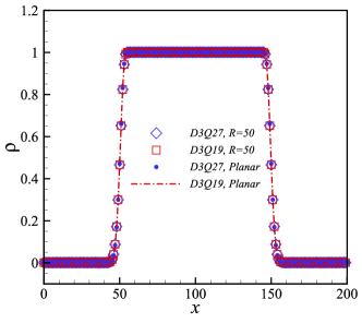
Figure 1: Comparison of the density profiles ( ${\rho_{v}}=0.001$ and ${\rho_{l}}=1.0$ ) at the Planar interfaces and circular interfaces (${R_{0}}=50$) by the non-orthogonal D3Q27 and D3Q19 MRT-LBMs. For the planar interfaces, the two methods reproduce very accurate coexistence densities. For the circular interfaces, the small discrepancies in the vapor phase are within 6 $\%$. The interface widths obtained by Eq. (21) are $5\leq W\leq 6$.

In the simulation, the square-root-form pseudopotential is used and the interaction strength parameter is fixed as $G=-1$. The density profiles along two planar interfaces in the $x$ direction by the D3Q27 and D3Q19 non-orthogonal MRT-LBMs are shown in Fig. 1. It is seen that the numerical coexistence densities are in very good agreement with the equilibrium vapor and liquid densities ( ${\rho_{v}}=0.001$ and ${\rho_{l}}=1.0$ ). A spherical droplet of radius ${R_{0}}=50$ (a representative radius in the following applications) is then initially located at the center of a $200\times 200\times 200$ cubic box to verify the thermodynamic consistency. The steady density profiles along the center line ($y=100,{\rm{}}z=100$) are also shown in Fig. 1 for comparison. The liquid density at ${R_{0}}=50$ is basically the same as the value at the planar interface, while the small discrepancies in the vapor phase are within 6 $\%$. Generally, the density ratio in our simulation is larger than 940. In addition, the interface width, $W$, can be measured by fitting the following curve to the density profile,

$$\rho(x)=\frac{{({\rho_{l}}+{\rho_{v}})}}{2}{\rm{+}}\frac{{({\rho_{l}}-{\rho_{v}})}}{2}\tanh\left[{\frac{{2(x-50)}}{W}}\right],~{}~{}x<=100.$$ (21)

The above equation can be rewritten as $W=({\rho_{l}}-{\rho_{v}})/(\partial\rho/\partial x){|_{x=50}}$ Fei et al. (2018b). Using the numerical differentiation, the interface widths for density profiles in Fig. 1 are obtained as, $5\leq W\leq 6$.

III.2 Evolution of spurious velocities

Spurious currents are usually viewed as an important cause of instability in the pseudopotential model. Here the average spurious velocity magnitude in the gas phase ${{{{\bar{u}}}}_{v}}$ Lycett-Brown and Luo (2014) is considered to compare the numerical performances of the proposed non-orthogonal MRT-LBMs and the classical SRT-LBM. The SRT-LBM is obtained by setting all the relaxation parameters equal to one another. The spurious velocity is measured based on the static droplet case in sec. III.1 at different viscosities. It may be noted that the dynamic viscosity ratio is ${\mu_{l}}/{\mu_{v}}=({\rho_{l}}/{\rho_{v}})\approx 1000$ in this simulation due to the unity kinematic viscosity, while different dynamic viscosity ratios can be used in the following applications.

From Table 2, it is seen that the present non-orthogonal MRT-LBM models help to reduce the spurious currents compared with SRT-LBM, and the D3Q27 model outperforms the D3Q19 model at low viscosities. In addition, we also provide the evolution of spurious kinetic energy for the case $\nu=0.02$ in Fig. 2. Here the spurious kinetic energy is calculated based on the global integral of the spurious velocities. The SRT-LBM case diverges after 1000 steps, while the present models allow us to achieve convergent results. Clearly, the proposed non-orthogonal MRT-LBM has superior numerical stability over the SRT-LBM.

Table 2: Average spurious velocity magnitude in the gas phase ${{{{\bar{u}}}}_{v}}$ produced by different methods.

methods	$\nu=0.075$	$\nu=0.05$	$\nu=0.02$	$\nu=0.01$
D3Q27 MRT	0.00116	0.00293	0.0172	0.0245
D3Q19 MRT	0.00085	0.00333	0.0180	0.0295
D3Q27 SRT	0.0150	0.06542	NaN	NaN

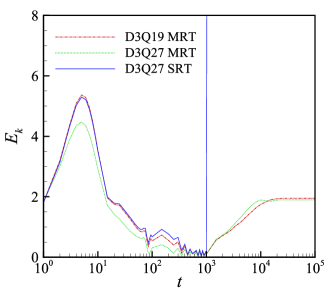
Figure 2: Evolution of spurious kinetic energy ${E_{k}}$ for a static droplet with $\nu=0.02$.

III.3 Realization of tunable surface tension

The adjustment of the surface tension is first verified by simulating droplets with a series of radii, ${R_{0}}=[28,33,38,43,48]$ , in a $180\times 180\times 180$ cubic box. According to the Laplace’s law, the pressure difference across a spherical interface is related to the droplet radius ${R_{0}}$ and the surface tension $\gamma$ via $\Delta p={p_{{\mathop{\rm int}}}}-{p_{out}}=2\gamma/{R_{0}}$. The obtained surface tensions at different $k$ are shown in Fig. 3a. As is shown, there is a good linear scaling between the surface tension and (1-$\kappa$), which confirms the theoretical analysis that surface tension can be reduced linearly with increasing parameter $k$ in Eq. (40). In addition, the numerical pressure differences at $\kappa$=0, 0.4, 0.6, and 0.8 by D3Q19 non-orthogonal MRT model are given in Fig. 3b. It can be seen that the numerical results agree well with the linear fit denoted by the solid lines. In the following simulations, we only adopt the D3Q19 model due to its smaller computational load.

In addition to the static case, we consider the decay of capillary waves between two fluids with equal viscosities ($\nu=0.01$), which is a classical test for the accuracy of numerical models for surface-tension-driven interfacial dynamics Shan and Chen (1994); Li and Luo (2013). The computational domain is in a cuboid of length $L$, height $H$ and depth $D$. For convenience, we use $D=5$ and impose periodic condition in the $z$ direction. As suggested in Shan and Chen (1994); Li and Luo (2013), the aspect ratio $H/L$ should be large enough and is chosen as 5 with $L=160$. The periodic and nonslip boundary conditions are adopted in the $x$ and $y$ directions, respectively. Initially, an interfacial disturbance is given in the middle of the cuboid of the form $y(x)={h_{0}}\cos(kx)$, where $k=2\pi/L$ is the wave number and ${h_{0}}=20$ is the wave amplitude. For the given surface tension, the dispersion relation of capillary wave is Shan and Chen (1994), ${\Theta^{2}}=\gamma{k^{3}}/({\rho_{l}}+{\rho_{v}})$. Figure 3c shows the evolution of the interface at $x=L/2$ for three cases by the present non-orthogonal MRT-LBM. We can clearly see that the dynamic decay of capillary waves can be well captured using the proposed method, and the oscillating period increases with the decrease of surface tension (increase of $k$). To be quantitative, we compare the measured oscillating period ${T^{*}}$ with the theoretical value $T=2\pi/\Theta$. Generally, the present results are in very good agreement with the analytical results, with relative errors of $0.8\%$, $1.0\%$ and $2.9\%$ for $k=0$, $k=0.4$ and $k=0.8$, respectively.

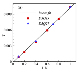
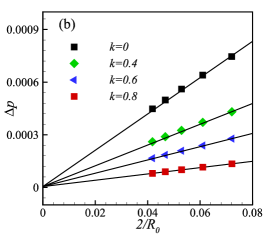
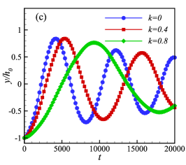
Figure 3: Verification of the surface tension adjustment method in Eq. (40). (a) and (b) are based on the static droplet case: (a) surface tensions achieved at different $k$; (b) numerical pressure difference as a function of $2/{R_{0}}$ at different $k$ by D3Q19 non-orthogonal MRT model. (c) Dynamic decay of capillary waves: for $k=[0,0.4,0.8]$, the analytical oscillation periods based on the surface tension by the static cases are $T=[7959,10504,19056]$, while the measured periods are ${T^{*}}=[8025,10400,18500]$, respectively.

III.4 Validation of spatial accuracy

To test the spatial accuracy of the proposed non-orthogonal MRT-LBM for multiphase flow, we conduct simulations of a static droplet with different mesh sizes, ${N_{x}}\times{N_{y}}\times{N_{z}}=100\times 100\times 100$, $200\times 200\times 200$, $300\times 300\times 300$, and $400\times 400\times 400$. The droplet radius is $R={N_{x}}/4$ and the periodic boundary conditions are imposed in all three directions. As suggested in Xu et al. (2015), we use the finest mesh as the standard case and calculate the relative error for the results on other meshes by $E({N_{x}})=\left|{\rho({N_{x}})-\rho(400)}\right|$, where ${\rho({N_{x}})}$ represents the convergent value of liquid/gas density on the mesh ${N_{x}}\times{N_{y}}\times{N_{z}}$. The changes in the relative error with the mesh size for different values of $k$ are shown in Fig. 4, where the top black line stands for the exact second-order accuracy. It is demonstrated that the present model has approximately second-order accuracy in space.

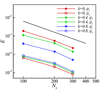
Figure 4: Changes in the relative error $E$ of steady densities with the mesh size ${N_{x}}$. The black solid line represents exact second-order accuracy. Three cases with different surface tensions ($k$) are considered.

III.5 Implementation of wettability conditions

Next, we consider the implementation of the wettability. For the pseudopotential model, various schemes to implement the contact angle between the fluid and solid phases have been proposed in the literature Huang et al. (2007); Li et al. (2014). In this work, we adopt a modified pseudopotential-based contact angle scheme Li et al. (2014), in which a fluid-solid interaction is defined as,

$${{\bf{F}}_{ads}}({\bf{x}})=-{G_{ads}}\psi({\bf{x}})\sum\limits_{i}{w({{\left|{{{\bf{e}}_{i}}}\right|}^{2}})}\psi({\bf{x}})s({\bf{x}}+{{\bf{e}}_{i}}\Delta t){{\bf{e}}_{i}}$$ (22)

where ${G_{ads}}$ is the fluid-solid interaction strength to adjust the contact angle, and $s({\bf{x}})$ is an indicator function, which is equal to 1 or 0 for a solid or a fluid phase, respectively. For such a treatment, ${G_{abs}}<0$ , ${G_{abs}}=0$ , and ${G_{abs}}>0$ recover the hydrophilic, neutral, and hydrophobic walls, respectively. However, there is still no analytical relation between the specified contact angle and the value of ${G_{ads}}$ . Usually, ${G_{ads}}$ is set to match the prescribed one. In the present work, the intrinsic contact angles are implemented without considering contact angle hysteresis. For cases where the three-phase contact line motion is a dominant factor Eddi, Winkels, and Snoeijer (2013); Mistry and Muralidhar (2018), alternative contact angle schemes, such as the geometric formulation Ding and Spelt (2007); Wang, Huang, and Lu (2013), should be adopted to include the contact angle hysteresis.

As a benchmark case, we choose ${G_{abs}}=0.23$, the measured contact angle is around ${157^{\circ}}$, which is a representative value for super-hydrophobic surfaces. To verify the implementation, a droplet impact on a solid wall is simulated. In this problem, the droplet spreads firstly to reach a maximal spreading diameter, then retracts to reduce its interfacial energy, and finally rebounds from the solid surface due to the relatively small energy loss by dissipation and friction. According to the universal scaling summarized by Richard et al. Richard, Clanet, and Quéré (2002), the contact time ${t_{c}}$ , a time period from when the droplet first touches the surface to that when it bounces off the surface, is proportional to the inertia-capillarity time,

$$\tau=\sqrt{{\rho_{l}}{{R_{0}}^{3}}/\gamma},$$ (23)

where the scale factor ${t^{*}}={t_{c}}/\tau\approx 2.2\pm 0.3$ is independent of the impact velocity $U$ and holds in a range of the Weber number, $We={\rho_{L}}{R_{0}}{U^{2}}/\gamma$ .

We consider a series of cases with the droplet radius $30\leq{R_{0}}\leq 50$ and surface tension $0.00395\leq\gamma\leq 0.01034$ ($0\leq\kappa\leq 0.6$). The resulting range of the inertia-capillarity time is $1616\leq\tau\leq 5625$ . The simulations are run in a domain of dimensions around 6${R_{0}}$. In Fig. 5a, we show the time evolution of the spreading film radius $R$ for a representative case with $W{\rm{e}}=27$, where we can see the present simulation is in good agreement with the experimental result reported in Bird et al. (2013). The contact time as a function of the inertia-capillarity time is shown in Fig. 5b. Within the considered range of parameters, a very good scaling ${\tau_{c}}/\tau{\rm{=}}2.26$ is achieved, which validates our implementation of wettability conditions, as well as the adjustment of surface tension.

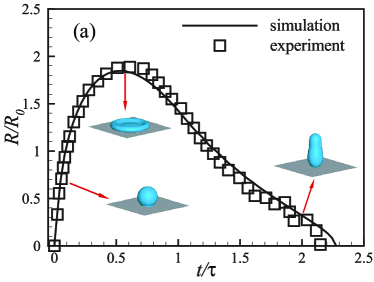
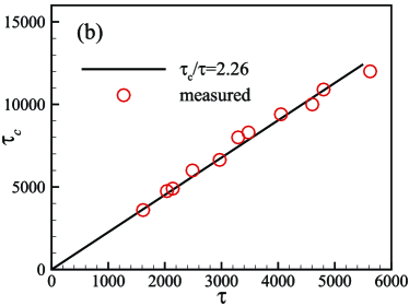
Figure 5: (a) Time evolution of the dimensionless film radius for a water droplet impacting on the superhydrophobic surface at $We=27$. Line: present simulation; symbols: experiment in Bird et al. (2013). Inset: typical snapshots during the impacting process. (b) Contact time ${\tau_{c}}$ as a function of the inertia-capillarity time $\tau$ for a droplet impacting on the superhydrophobic surface.

IV Numerical applications in realistic multiphase flows

IV.1 Fuel droplet impact on a solid surface

Fuel droplet impact on a solid surface occurs in fuel spray in engines, spray cooling, and inking jet printing Moreira, Moita, and Panao (2010). As discussed in the literature, the impact outcome depends on the properties of both the fuel droplet and the surface Moreira, Moita, and Panao (2010). Here we consider the ethanol droplet and diesel fuel droplet impact on hydrophilic surface. The simulation configuration is that a droplet with radius ${R_{0}}$ and velocity $U$ impact on the solid wall vertically (in the $z$ direction). The simulations results by the present non-orthogonal MRT-LBM are compared with the experimental data provided in Ref. Moita and Moreira (2007) and a recent smoothed particle hydrodynamics (SPH) simulation Yang, Dai, and Kong (2017). In the present work, the effect of temperature, such as the phase change process during drop impact on heated surfacesYang et al. (2019), is not considered. For methods of incorporating thermal effects into multiphase LBM, the interested readers are kindly directed to Ref. Li et al. (2016).

The physical properties of the ethanol and diesel have been provided in Ref. Moita and Moreira (2007). Due to the large density ratio for both the two fuel droplets compared with the ambient gas. The density ratio is fixed to be the same with the previous setting. The experimental dynamic viscosity ratio ${\mu_{l}}/{\mu_{v}}$ can be achieved by tuning the vapor-liquid kinematic viscosity ratio ${\nu_{l}}/\nu{{}_{v}}$ through a variable relaxation time, i.e.,

$$\nu={\nu_{v}}+({\nu_{l}}-{\nu_{v}})\frac{{\rho-{\rho_{v}}}}{{{\rho_{l}}-{\rho_{v}}}}.$$ (24)

Remarkably, the impact Reynolds number ${\rm{Re}}={\rho_{l}}{R_{0}}U/{\mu_{l}}$ and Weber number $We={\rho_{l}}{U^{2}}{R_{0}}/\gamma$ in the present method can be tuned independently via the adjustments of the surface tension and the viscosity to match the experimental conditions. It may be noted that the Reynolds and Weber numbers are defined based on the droplet radius ${R_{0}}$ throughout this paper, while the droplet diameter $D=2{R_{0}}$ has also been commonly adopted in the literature. The fluid-solid interaction strength is set to ${G_{ads}}=-0.1$ to match the wettability condition Yang, Dai, and Kong (2017).

The first simulation is an impact case by the ethanol drop. In the experiment, the droplet radius and impact velocity are ${R_{E}}=1.2mm$ and ${U_{E}}=3.1m/s$. According to the physical properties Yang, Dai, and Kong (2017), the corresponding Reynolds and Weber numbers are around ${\mathop{\rm Re}\nolimits}=2500$ and $We=410$, respectively. In the simulation, we choose ${R_{0}}=70$, $U=0.125$ and ${\nu_{l}}=0.0035$. The simulation is run in a domain around $9R\times 9R\times 3.5R$, where the periodic boundary conditions are used in the $x$ and $y$ directions and the non-slip boundary conditions on the top and bottom walls. Figure 6 shows the predicted evolution of the droplet impacting process. Specifically, the liquid droplet spreads out onto the solid wall and gradually forms a thin liquid film without splashing, which is consistent with the experimental observation Moita and Moreira (2007). For comparison, the SPH simulation result in Yang, Dai, and Kong (2017) is also shown in Figure 6. As expected, the present film is smoother than the SPH simulation. It should be noted that the rough boundaries in the film by SPH are not the secondary droplets due to splashing, as mentioned in Yang, Dai, and Kong (2017).

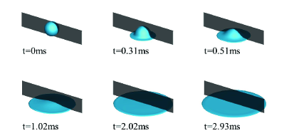
(a)

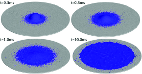
(b)

Figure 6: Snapshots of an ethanol drop impinging on a drying surface (${R_{E}}=1.2mm$, ${U_{E}}=3.1m/s$): (a) the present non-orthogonal MRT-LBM simulation; (b) SPH simulation in Yang, Dai, and Kong (2017).

The diameter of the spreading film ${D_{f}}$ is then measured. To compare with the experimental data, we can convert the lattice time and spreading film diameter to the experimental units using the dimensionless time and length scales, ${t^{*}}=tU/{R_{0}}$ and ${\delta^{*}}={D_{f}}/{R_{0}}$. The predicted spreading diameter, as a function of time, compared with the experimental measurement and SPH simulation, is shown in Fig. 7. In addition, another impact case for diesel droplet (${R_{E}}=1.3mm$ and ${U_{E}}=3.1$) is also shown in Fig. 7. Due to the smaller Reynolds and Weber numbers (${\mathop{\rm Re}\nolimits}=930$ and $We=350$), ${R_{0}}=50$ is used to simulate the diesel droplet impingement and a video for this case is provided in the supplementary movie 1. It can be seen in Fig. 7 that the present simulation results are generally in good agreement with the previous data Moita and Moreira (2007); Yang, Dai, and Kong (2017). More specifically, the spreading diameters by the present method are smaller than the SPH results in the later stages and seem to be more consistent with the experimental results.

In addition, we find that for the cases considered here with large Reynolds and Weber numbers, the SRT scheme always leads to divergence shortly after the droplet lands on the wall, which further confirms the improved numerical stability of the proposed non-orthogonal MRT scheme.

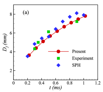
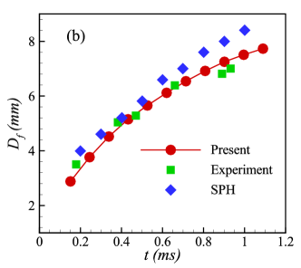
Figure 7: The spreading diameters as a function of time by the present simulation, experimental measurement Moita and Moreira (2007) and SPH simulation Yang, Dai, and Kong (2017): (a) ethanol drop impact (${R_{E}}=1.2mm$ and ${U_{E}}=3.1$); (b) diesel drop impact (${R_{E}}=1.3mm$ and ${U_{E}}=3.1$).

IV.2 Droplet impact on a super-hydrophobic wall with a cylindrical obstacle

Reducing the contact time for a droplet impact on a super-hydrophobic solid surface plays an important role in a broad range of realistic applications, such as self-cleaning, anti-icing and dropwise condensation Liu et al. (2015, 2014); Andrew, Liu, and Yeomans (2017). Recently, several methods have been demonstrated to reduce the contact time Liu et al. (2015, 2014); Gauthier et al. (2015). In this paper, we consider the approach by installing a cylinder on a super-hydrophobic solid surface, while the cylinder has the same wettability with the solid surface. As analyzed by Liu et al. Liu et al. (2015), when a droplet lands, more momentum is transferred into the azimuthal direction of the cylinder rather than the axial direction. As a result, the droplet remains extended in the azimuthal direction when it begins to retract along the axial direction. It is the dynamically asymmetric momentum and mass distribution that reduces the total contact time during the impact process.

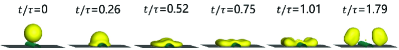
(a)

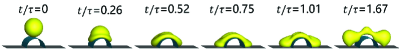
(b)

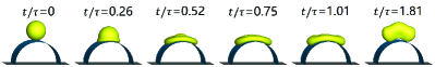
(c)

Figure 8: Snapshots for a droplet impact on a super-hydrophobic surface with a cylindrical obstacle by the present simulation: (a) $R/{R_{0}}=0.4$, rebounce at ${t^{*}}\approx 1.79$; (b) $R/{R_{0}}=1.0$, rebounce at ${t^{*}}\approx 1.67$; (c) $R/{R_{0}}=2.3$, rebounce at ${t^{*}}\approx 1.81$.

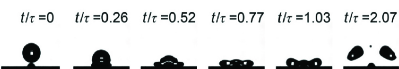
(a)

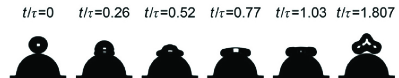
(b)

Figure 9: Experiment measurements for a droplet hitting a cylinder Liu et al. (2015); Andrew, Liu, and Yeomans (2017): (a) $R/{R_{0}}=0.4$ and (b) $R/{R_{0}}=2.3$.

In the simulation, the droplet radius is fixed at ${R_{0}}=50$, and a series cases with the cylinder radii $10\leq R\leq 120$ are considered. The simulations are carried out in a box around $6{R_{0}}\times 6{R_{0}}\times 5{R_{0}}$, with periodic boundaries along $x$ and $y$ directions, and non-slip boundary conditions on the top and bottom, as well as the cylinder surface. The liquid viscosity is set to ${\nu_{l}}=0.0075$ and $Oh=({\rho_{l}}{\nu_{l}})/\sqrt{{\rho_{l}}\gamma{R_{0}}}<0.015$ for two Weber numbers, $We=10$ and $20$. The gravity is neglected since all the simulations are below the inertial capillary length scale. The fluid-solid interaction parameter ${G_{ads}}=0.23$ is used to implement a static contact angle $\theta\approx{157^{\circ}}$. A reference case without the cylinder is simulated first and the dimensionless contact time is $t/\tau\approx 2.35$, which is in good agreement with the universal scaling Richard, Clanet, and Quéré (2002).

Figure 8 shows snapshots for three representative cases, $R<{R_{0}}$, $R={R_{0}}$, and $R>{R_{0}}$ at $We=10$. For the case $R/{R_{0}}=0.4$, the droplet spreads onto the plat surface soon after the impact due to the small cylinder radius. Thus only a small part of the droplet is on the cylinder ridge and this small central part retracts quickly while the main part is still spreading. This results in a central pinch-off, splitting the droplet into two parts on each side of the cylinder and a small satellite. The small satellite is unsteady and lifts off immediately and the two parts finally rebound at $t/\tau=1.79$. The impact process is in very good agreement with the experiment phenomena shown in Fig. 9 and a video for this case is provided in the supplementary movie 2. For the medium cylinder at $R/{R_{0}}=1.0$, a smaller part of the droplet spreads onto the plat surface and the droplet cannot be split into two parts despite the significant deformation. Shortly after the completion of axial retraction, the droplet bounces. Moreover, for the large cylinder radius at $R/{R_{0}}=2.3$, the droplet film changes to be approximately elliptical in the early stage due to the momentum imbalance. More specifically, more momentum is transferred in the azimuthal direction than the axial direction, as analyzed by Liu et al. Liu et al. (2015). Then the drop retracts first in the axial direction while keeping extending around the cylinder. Once the axial retraction is complete, the droplet bounces. The dynamic process is consistent with the experiment phenomena shown in Fig. 9. It should be noted that the difference between the last snapshots in Fig. 8a and Fig. 9a is because the two snapshots are taken at different instants in the evolution.

Figure. 10 presents the variation of the dimensionless contact time ${t^{*}}={t_{c}}/\tau$ as a function of the dimensionless cylinder radius ${R^{*}}=R/{R_{0}}$ at $We=10$ and $20$. Generally, it can be seen that the contact time is minimized at ${R^{*}}\approx 1$. Moreover, the figure is asymmetric, where the contact time decreases quickly from ${R^{*}}=0$ to ${R^{*}}\approx 1$ while it increases slowly at ${R^{*}}>1$. The trend predicted by the present simulation agrees well with previous studies Liu et al. (2015); Andrew, Liu, and Yeomans (2017). In addition, it may be noted that the contact time for droplet hitting small wires (${R^{*}}<0.1$) may be reduced by quite different physical mechanisms and this range is not covered in Fig. 10. For example, Gauthier et al. Gauthier et al. (2015) showed that the contact time for a droplet impact on a small wire scales inversely as the square root of the number of lobes produced.

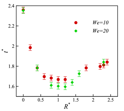
Figure 10: Variation of the dimensionless contact time ${t^{*}}={t_{c}}/\tau$ as a function of the dimensionless cylinder radius ${R^{*}}=R/{R_{0}}$.

Finally, the conservation of volume or mass in our simulations is considered, which is an important factor affecting the accuracy of simulations involving breakup and/or merging of the phase interfaces Aniszewski, Menard, and Marek (2014). In Fig. 11, we show the evolution of dimensionless volume for the liquid phase in the three cases considered in Fig. 8. It is seen that the three cases show similar tendency: the volume increases slightly in the early stage and then decreases gradually to a steady value and the fluctuation is approximately within $\pm 1\%$. This is within the error margin of estimating the volume of complex shapes. In our simulations, we also find that the small secondary droplet produced in Fig. 8a is going to be smaller and smaller, and disappear in the end, which is similar to the interface diffusion phenomenon mentioned in Gong, Yan, and Chen (2018) and leads to slight loss of liquid volume. Generally, it is demonstrated that the present model performs well in terms of global volume conservation.

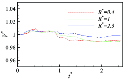
Figure 11: Evolution of dimensionless volume for the liquid phase for three cases at $We=10$.

V Conclusions

Through theoretical analysis, a generalized non-orthogonal multiple-relaxation-time lattice Boltzmann method (MRT-LBM) based on an improved moment set Fei, Luo, and Li (2018) is developed and proved to reproduce the macroscopic Navier-Stokes equations in the low Mach number limit. Compared with the classical MRT-LBM, the numbers of non-zeros in the present transformation matrix ${\bf{M}}$ and its inverse matrix ${{\bf{M}}^{{\rm{-}}1}}$ are much reduced, leading to a simplified implementation and an enhanced computational efficiency in the present method. Moreover, a non-orthogonal MRT-LBM based on a sub-lattice (e.g., D3Q19) can be extracted from the method on the full-lattice (D3Q27) directly, which shows that the proposed non-orthogonal MRT-LBM exhibits good portability across lattices.

The proposed method is further extended to simulate multiphase flows with large density ratio and tunable surface tension, and validated through benchmark cases. It is finally applied to two practical problems, a fuel droplet impacting on a dry surface at high Reynolds and Weber numbers and a droplet impacting on a super-hydrophobic wall with a cylindrical obstacle, achieving satisfactory agreement with recent experimental and numerical data.

Supplementary Material

See supplementary material for the explicit expressions of ${\bf{M}}$ and ${{\bf{M}}^{-1}}$ and supplementary movies.

Appendix A Chapman-Enskog analysis

Using Eq. (4) and the relation ${f_{i}}{\rm{=}}{{\bar{f}}_{i}}{\rm{+}}\Delta t{{\bar{F}}_{i}}/2$, a second-order Taylor series expansion of Eq. (9) at $({\bf{x}},t)$ yields

$$\Delta t({\partial_{t}}+{{\bf{e}}_{i}}\cdot\nabla){f_{i}}+\frac{{\Delta{t^{2}}}}{2}{({\partial_{t}}+{{\bf{e}}_{i}}\cdot\nabla)^{2}}{f_{i}}+O(\Delta{t^{3}})=-{\Lambda_{i,k}}({f_{k}}-f_{k}^{eq})+\Delta t{{\bar{F}}_{i}}+\frac{{\Delta{t^{2}}}}{2}({\partial_{t}}+{{\bf{e}}_{i}}\cdot\nabla){{\bar{F}}_{i}}.$$ (25)

Multiplying Eq. (25) by the transformation matrix ${\bf{M}}$ leads to the following equation

$$({\bf{I}}{\partial_{t}}+{\bf{D}}){\bf{m}}+\frac{{\Delta t}}{2}{({\bf{I}}{\partial_{t}}+{\bf{D}})^{2}}{\bf{m}}+O(\Delta{t^{2}})=-\frac{{\bf{S}}}{{\Delta t}}({\bf{m}}-{{\bf{m}}^{eq}})+{\bf{\tilde{F}}}+\frac{{\Delta t}}{2}({\bf{I}}{\partial_{t}}+{\bf{D}}){\bf{\tilde{F}}}$$ (26)

Where ${\bf{D}}={{\bf{C}}_{x}}{\partial_{x}}+{{\bf{C}}_{y}}{\partial_{y}}+{{\bf{C}}_{z}}{\partial_{z}}$, in which ${{\bf{C}}_{a}}={\bf{M}}{{\bf{E}}_{a}}{{\bf{M}}^{-1}}$ with ${{\bf{E}}_{a}}=diag[{{\bf{e}}_{0,a}},{{\bf{e}}_{1,a}},...,{{\bf{e}}_{26,a}}]$ for $a=x,y,z$. By introducing the following Chapman-Enskog expansions,

$${\partial_{t}}=\varepsilon{\partial_{t1}}+{\varepsilon^{2}}{\partial_{t2}}{\rm{+}}...,{\bf{D}}{\rm{=}}\varepsilon{{\bf{D}}_{1}},{\bf{m}}={{\bf{m}}^{eq}}+\varepsilon{{\bf{m}}^{(1)}}+{\varepsilon^{2}}{{\bf{m}}^{(2)}}+...,{\bf{\tilde{F}}}=\varepsilon{{\bf{\tilde{F}}}^{(1)}},$$ (27)

Eq. (26) can be rewritten in the consecutive orders of the expansion parameter $\varepsilon$ as follows:

$$O(\varepsilon):({\bf{I}}{\partial_{t1}}+{{\bf{D}}_{1}}){{\bf{m}}^{eq}}=-\frac{{\bf{S}}}{{\Delta t}}{{\bf{m}}^{(1)}}+{{\bf{\tilde{F}}}^{(1)}},$$ (28a)

$$O({\varepsilon^{2}}):{\partial_{t2}}{{\bf{m}}^{eq}}+({\bf{I}}{\partial_{t1}}+{{\bf{D}}_{1}}){{\bf{m}}^{(1)}}+\frac{{\Delta t}}{2}{({\bf{I}}{\partial_{t1}}+{{\bf{D}}_{1}})^{2}}{{\bf{m}}^{eq}}=-\frac{{\bf{S}}}{{\Delta t}}{{\bf{m}}^{(2)}}+\frac{{\Delta t}}{2}({\bf{I}}{\partial_{t1}}+{{\bf{D}}_{1}}){{{\bf{\tilde{F}}}}^{(1)}}.$$ (28b)

Using the first-order $O(\varepsilon)$ equation, the second-order $O({\varepsilon^{2}})$ can be simplified as

$$O({\varepsilon^{2}}):{\partial_{t2}}{{\bf{m}}^{eq}}+({\bf{I}}{\partial_{t1}}+{{\bf{D}}_{1}})({\bf{I}}-\frac{{\bf{S}}}{2}){{\bf{m}}^{(1)}}=-\frac{{\bf{S}}}{{\Delta t}}{{\bf{m}}^{(2)}}.$$ (29)

According to Eq. (28a) and the definition in Eq. (14), we can obtain continuity and momentum equations at $O(\varepsilon)$ level,

$$\begin{array}[]{*{20}{c}}{{\partial_{t1}}\rho+{\partial_{x1}}(\rho{u_{x}})+{\partial_{y1}}(\rho{u_{y}})+{\partial_{z1}}(\rho{u_{z}})=0,}\\ {{\partial_{t1}}(\rho{u_{x}})+{\partial_{x1}}(\rho c_{s}^{2}+\rho u_{x}^{2})+{\partial_{y1}}(\rho{u_{x}}{u_{y}})+{\partial_{z1}}(\rho{u_{x}}{u_{z}})=F_{x}^{(1)},}\\ {{\partial_{t1}}(\rho{u_{y}})+{\partial_{x1}}(\rho{u_{x}}{u_{y}})+{\partial_{y1}}(\rho c_{s}^{2}+\rho u_{y}^{2})+{\partial_{z1}}(\rho{u_{y}}{u_{z}})=F_{y}^{(1)},}\\ {{\partial_{t1}}(\rho{u_{z}})+{\partial_{x1}}(\rho{u_{x}}{u_{z}})+{\partial_{y1}}(\rho{u_{y}}{u_{z}})+{\partial_{z1}}(\rho c_{s}^{2}+\rho u_{z}^{2})=F_{z}^{(1)},}\\ \end{array}$$ (30)

Analogously, the continuity and $x$ direction momentum equations at $O({\varepsilon^{2}})$ level can be obtained from Eq. (29)

$${\partial_{t2}}\rho=0,$$ (31a)

$${\partial_{t2}}(\rho{u_{x}})+\frac{1}{3}{\partial_{x1}}\left[{(1-\frac{{{s_{b}}}}{2})m_{7}^{(1)}+(1-\frac{{{s_{\nu}}}}{2})m_{8}^{(1)}+(1-\frac{{{s_{\nu}}}}{2})m_{9}^{(1)}}\right]+{\partial_{y1}}\left[{(1-\frac{{{s_{\nu}}}}{2})m_{4}^{(1)}}\right]+{\partial_{z1}}\left[{(1-\frac{{{s_{\nu}}}}{2})m_{5}^{(1)}}\right]=0,$$ (31b)

where the unknown first-order non-equilibrium moments can be obtained according to Eq. (28a),

$$\begin{array}[]{*{20}{c}}{\partial_{t1}}m_{4}^{eq}+{\partial_{x1}}m_{12}^{eq}+{\partial_{y1}}m_{10}^{eq}+{\partial_{z1}}m_{16}^{eq}=-{s_{\nu}}m_{4}^{(1)}/\Delta t+\tilde{F}_{4}^{(1)},\\ {{\partial_{t1}}m_{5}^{eq}+{\partial_{x1}}m_{13}^{eq}+{\partial_{y1}}m_{16}^{eq}+{\partial_{z1}}m_{11}^{eq}=-{s_{\nu}}m_{5}^{(1)}/\Delta t+\tilde{F}_{5}^{(1)},}\\ {{\partial_{t1}}m_{7}^{eq}+{\partial_{x1}}(m_{1}^{eq}+m_{10}^{eq}+m_{11}^{eq})+{\partial_{y1}}(m_{2}^{eq}+m_{12}^{eq}+m_{14}^{eq})+{\partial_{z1}}(m_{3}^{eq}+m_{13}^{eq}{\rm{+}}m_{15}^{eq})=-{s_{b}}m_{7}^{(1)}/\Delta t+\tilde{F}_{7}^{(1)},}\\ {{\partial_{t1}}m_{8}^{eq}+{\partial_{x1}}(m_{1}^{eq}-m_{10}^{eq})+{\partial_{y1}}(-m_{2}^{eq}+m_{12}^{eq})+{\partial_{z1}}(m_{13}^{eq}-m_{15}^{eq})=-{s_{\nu}}m_{8}^{(1)}/\Delta t+\tilde{F}_{8}^{(1)},}\\ {{\partial_{t1}}m_{9}^{eq}+{\partial_{x1}}(m_{1}^{eq}-m_{11}^{eq})+{\partial_{y1}}(m_{12}^{eq}-m_{14}^{eq})+{\partial_{z1}}(-m_{3}^{eq}+m_{13}^{eq})=-{s_{\nu}}m_{9}^{(1)}/\Delta t+\tilde{F}_{9}^{(1)},}\\ \end{array}$$ (32)

Here, the following relations can be obtained according to Eq. (30),

$${\partial_{t1}}(\rho{u_{\alpha}}{u_{\beta}})={u_{\alpha}}{\partial_{t1}}(\rho{u_{\beta}})+{u_{\beta}}{\partial_{t1}}(\rho{u_{\alpha}})-{u_{\alpha}}{u_{\beta}}{\partial_{t1}}(\rho)\approx-{u_{\alpha}}{\partial_{\beta 1}}(\rho c_{s}^{2})-{u_{\beta}}{\partial_{a1}}(\rho c_{s}^{2})+{u_{\alpha}}F_{\beta}^{(1)}+{u_{\beta}}F_{\alpha}^{(1)}$$ (33)

Substituting the above relations into Eq. (32), the first-order non-equilibrium moments in Eq. (31b) can be written explicitly,

$$\begin{array}[]{l}m_{4}^{(1)}=-\frac{{\Delta t}}{{{s_{\nu}}}}\rho c_{s}^{2}({\partial_{x1}}{u_{y}}+{\partial_{y1}}{u_{x}}),~{}m_{5}^{(1)}=-\frac{{\Delta t}}{{{s_{\nu}}}}\rho c_{s}^{2}({\partial_{x1}}{u_{z}}+{\partial_{z1}}{u_{x}}),~{}m_{7}^{(1)}=-\frac{{2\Delta t}}{{{s_{b}}}}\rho c_{s}^{2}({\partial_{x1}}{u_{x}}+{\partial_{y1}}{u_{y}}+{\partial_{z1}}{u_{z}}),\\ m_{8}^{(1)}=-\frac{{2\Delta t}}{{{s_{\nu}}}}\rho c_{s}^{2}({\partial_{x1}}{u_{x}}-{\partial_{y1}}{u_{y}}),~{}m_{9}^{(1)}=-\frac{{2\Delta t}}{{{s_{\nu}}}}\rho c_{s}^{2}({\partial_{x1}}{u_{x}}-{\partial_{z1}}{u_{z}}).\\ \end{array}$$ (34)

Thus Eq. (31b) can be rewritten as

$$\begin{array}[]{l}{\partial_{t2}}(\rho{u_{x}})={\partial_{x1}}\left[{\rho{\nu_{b}}({\nabla_{1}}\cdot{\bf{u}})+\frac{2}{3}\rho\nu(2{\partial_{x1}}{u_{x}}-{\partial_{y1}}{u_{y}}-{\partial_{z1}}{u_{z}})}\right]\\ +{\partial_{y1}}\left[{\rho\nu({\partial_{y1}}{u_{x}}+{\partial_{x1}}{u_{y}})}\right]+{\partial_{z1}}\left[{\rho\nu({\partial_{z1}}{u_{x}}+{\partial_{x1}}{u_{z}})}\right],\\ \end{array}$$ (35)

where the kinematic viscosity and bulk viscosity are given by

$$\nu=c_{s}^{2}(\frac{1}{{{s_{\nu}}}}-\frac{1}{2})\Delta t,~{}~{}{\nu_{b}}=\frac{2}{3}c_{s}^{2}(\frac{1}{{{s_{b}}}}-\frac{1}{2})\Delta t.$$ (36)

Similarly, the momentum equations in $y$ and $z$ directions at $O({\varepsilon^{2}})$ level are given as

$$\begin{array}[]{l}{\partial_{t2}}(\rho{u_{y}})={\partial_{x1}}\left[{\rho\nu({\partial_{y1}}{u_{x}}+{\partial_{x1}}{u_{y}})}\right]+{\partial_{y1}}\left[{\rho{\nu_{b}}({\nabla_{1}}\cdot{\bf{u}})+\frac{2}{3}\rho\nu(2{\partial_{y1}}{u_{y}}-{\partial_{x1}}{u_{x}}-{\partial_{z1}}{u_{z}})}\right]\\ +{\partial_{z1}}\left[{\rho\nu({\partial_{z1}}{u_{y}}+{\partial_{y1}}{u_{z}})}\right]\\ {\partial_{t2}}(\rho{u_{z}})={\partial_{x1}}\left[{\rho\nu({\partial_{z1}}{u_{x}}+{\partial_{x1}}{u_{z}})}\right]+{\partial_{y1}}\left[{\rho\nu({\partial_{z1}}{u_{y}}+{\partial_{y1}}{u_{z}})}\right]\\ +{\partial_{z1}}\left[{\rho{\nu_{b}}({\nabla_{1}}\cdot{\bf{u}})+\frac{2}{3}\rho\nu(2{\partial_{z1}}{u_{z}}-{\partial_{x1}}{u_{x}}-{\partial_{y1}}{u_{y}})}\right].\\ \end{array}$$ (37)

Combining the $O({\varepsilon})$ level and $O({\varepsilon^{2}})$ level equations using the expansion relations in Eq. (27), we can obtain,

$$\begin{array}[]{l}{\partial_{t}}\rho+\nabla\cdot(\rho{\bf{u}})=0,\\ {\partial_{t}}(\rho{\bf{u}})+\nabla\cdot(\rho{\bf{uu}})=-\nabla(\rho c_{s}^{2})+\nabla\cdot\left[{\rho\nu(\nabla{\bf{u}}+{{(\nabla{\bf{u}})}^{\rm T}})-\frac{2}{3}\rho\nu(\nabla\cdot{\bf{u}}){\bf{I}}}\right]+\nabla\left[{\rho{\nu_{b}}(\nabla\cdot{\bf{u}})}\right]+{\bf{F}}.\\ \end{array}$$ (38)

From the above Chapman-Enskog analysis, we can see that the Navier-Stokes equations can be correctly recovered from the present non-orthogonal MRT-LB model in the low Mach number limit.

Appendix B Pseudopotential Multiphase model with high density ratio and tunable surface tension

When the square-root-form pseudopotential is used, the mechanical stability condition can not be accurately satisfied in the pseudopotential model. To solve this problem, Li et al. proposed a modified forcing scheme to adjust the mechanical stability condition Li et al. (2012); Li, Luo, and Li (2013). In addition, the original Shan-Chen pseudopotential model also suffers from the problem that the surface tension cannot be tuned independently of the density ratio. Li et al. developed another method to tune the surface tension in the 2D MRT LBM by incorporating a source term into the LB equation Li and Luo (2013). Due to the simplicity and efficiency, the above mentioned methods Li et al. (2012); Li, Luo, and Li (2013); Li and Luo (2013) have been adopted by different researchers Xu et al. (2015); Gong, Chen, and Yan (2017); Xu, Shyy, and Zhao (2017). Inspired by Li et al. Li et al. (2012); Li, Luo, and Li (2013); Li and Luo (2013), to achieve large density ratio and tunable surface tension in the present non-orthogonal MRT-LBM, several elements in ${\bf{\tilde{F}}}$ can be modified as,

$$\begin{array}[]{l}\tilde{F}_{4}^{{}^{\prime}}={{\tilde{F}}_{4}}-\frac{{{Q_{xy}}}}{{(s_{\nu}^{-1}-0.5)\Delta t}},~{}~{}\tilde{F}_{5}^{{}^{\prime}}={{\tilde{F}}_{5}}-\frac{{{Q_{xz}}}}{{(s_{\nu}^{-1}-0.5)\Delta t}},~{}~{}\tilde{F}_{6}^{{}^{\prime}}={{\tilde{F}}_{6}}-\frac{{{Q_{yz}}}}{{(s_{\nu}^{-1}-0.5)\Delta t}},\\ \tilde{F}_{7}^{{}^{\prime}}={{\tilde{F}}_{7}}+\frac{{6\sigma{{\left|{{{\bf{F}}_{{\mathop{\rm int}}}}}\right|}^{2}}}}{{{\psi^{2}}(s_{e}^{-1}-0.5)\Delta t}}+\frac{{4({Q_{xx}}+{Q_{yy}}+{Q_{zz}})}}{{5(s_{e}^{-1}-0.5)\Delta t}},~{}~{}\tilde{F}_{8}^{{}^{\prime}}={{\tilde{F}}_{8}}-\frac{{({Q_{xx}}-{Q_{yy}})}}{{(s_{\nu}^{-1}-0.5)\Delta t}},~{}~{}\tilde{F}_{9}^{{}^{\prime}}={{\tilde{F}}_{9}}-\frac{{({Q_{xx}}-{Q_{zz}})}}{{(s_{\nu}^{-1}-0.5)\Delta t}},\\ \end{array}$$ (39)

where the parameter $\sigma$, usually within $0.0625\leq\sigma\leq 0.125$, is employed to adjust the mechanical stability condition and its exact value can be determined by fitting the liquid-gas coexistence densities. The variable ${Q_{\alpha\beta}}$ is obtained via Li and Luo (2013),

$${Q_{\alpha\beta}}=\kappa\frac{G}{2}\psi({\bf{x}})\sum\limits_{i}{w({{\left|{{{\bf{e}}_{i}}}\right|}^{2}})}\left[{\psi({\bf{x}}+{{\bf{e}}_{i}}\Delta t)-\psi({\bf{x}})}\right]{{\rm{e}}_{i\alpha}}{e_{i\beta}},$$ (40)

where the parameter $\kappa$ is used to tune the surface tension. Consistent with Eq. (16), only the nearest or single-range neighboring nodes are needed in the calculation of ${Q_{\alpha\beta}}$, thus no additional computational complexity is introduced even at the boundary nodes.

In the Chapman analysis, the above modifications do not affect the equations at $O({\varepsilon})$ level. For the equations at $O({\varepsilon^{2}})$ level, it can be seen that Eq. (34) is changed due to the modifications of in the forcing terms. As a result, Eq. (35) is changed correspondingly,

$$\begin{array}[]{l}{\partial_{t2}}(\rho{u_{x}})={\partial_{x1}}\left[{\rho{\nu_{b}}({\nabla_{1}}\cdot{\bf{u}})+\frac{2}{3}\rho\nu(2{\partial_{x1}}{u_{x}}-{\partial_{y1}}{u_{y}}-{\partial_{z1}}{u_{z}})-\frac{{2\sigma{{\left|{{\bf{F}}_{{\mathop{\rm int}}}^{(1)}}\right|}^{2}}}}{{{\psi^{2}}}}+(\frac{2}{5}{Q_{xx1}}-\frac{3}{5}{Q_{yy1}}-\frac{3}{5}{Q_{zz1}})}\right]\\ {\rm{}}+{\partial_{y1}}\left[{\rho\nu({\partial_{y1}}{u_{x}}+{\partial_{x1}}{u_{y}})+{Q_{xy1}}}\right]+{\partial_{z1}}\left[{\rho\nu({\partial_{z1}}{u_{x}}+{\partial_{x1}}{u_{z}})+{Q_{xz1}}}\right].\\ \end{array}$$ (41)

The Taylor expansions of the interaction force ${{\bf{F}}_{{\mathop{\rm int}}}}$ and the term ${\bf{Q}}$ yield Li et al. (2012); Li and Luo (2013); Xu et al. (2015)

$${{\bf{F}}_{{\mathop{\rm int}}}}=-G{c^{2}}\left[{\psi\nabla\psi+\frac{1}{6}{c^{2}}\psi\nabla({\nabla^{2}}\psi)+...}\right],~{}~{}{\bf{Q}}=\frac{1}{{12}}\kappa G{c^{4}}\left[{\psi{\nabla^{2}}\psi{\bf{I}}+2\psi\nabla\nabla\psi+...}\right]$$ (42)

Substituting Eq. (42) into Eq. (41) and combining the correspondingly modified equations in y and z directions, the macroscopic momentum equation in Eq. (41) is rewritten as,

$$\begin{array}[]{*{20}{c}}{{\partial_{t}}(\rho{\bf{u}})+\nabla\cdot(\rho{\bf{uu}})=-\nabla(\rho c_{s}^{2})+\nabla\cdot\left[{\rho\nu(\nabla{\bf{u}}+{{(\nabla{\bf{u}})}^{\rm{T}}})-\frac{2}{3}\rho\nu(\nabla\cdot{\bf{u}}){\bf{I}}}\right]+\nabla\left[{\rho{\nu_{b}}(\nabla\cdot{\bf{u}})}\right]+{\bf{F}}}\\ {-2G^{2}{c^{4}}\sigma\nabla\cdot\left({{{\left|{\nabla\psi}\right|}^{2}}{\bf{I}}}\right)-\nabla\cdot\left[{\kappa\frac{{G{c^{4}}}}{6}(\psi{\nabla^{2}}\psi{\bf{I}}-\psi\nabla\nabla\psi)}\right].}\\ \end{array}$$ (43)

Following the standard approach by Shan Shan (2008), it can be shown that the surface tension coefficient finally reads Li and Luo (2013); Xu et al. (2015)

$$\gamma=\int_{-\infty}^{\infty}{({p_{0}}-{p_{T}})dx}=-\frac{{G{c^{4}}(1-\kappa)}}{6}\int_{{\rho_{g}}}^{{\rho_{l}}}{\psi{{}^{\prime 2}}(\frac{{d\rho}}{{dx}})d}\rho$$ (44)

where the integral extends across a planar interface normal to the $x$ direction, ${p_{0}}$ is the normal pressure tensor, ${p_{T}}$ is the transversal pressure tensor, and $\psi^{\prime}=d\psi/d\rho$ . From the above, it is shown that the surface tension $\gamma$ is proportional to $(1-\kappa)$ and can be tuned independently of the density ratio.

Appendix C D3Q19 non-orthogonal MRT-LBM

For the D3Q19 lattice, the discrete velocities ${{\bf{e}}_{j}}=[\left|{{e_{jx}}}\right\rangle,\left|{{e_{jy}}}\right\rangle,\left|{{e_{jz}}}\right\rangle]$ ($j=0,1,..,18$) are the first 19 elements in the D3Q27 lattice,

$$\begin{array}[]{l}\left|{{e_{jx}}}\right\rangle={\left[{0,{\rm{1}},-{\rm{1}},{\rm{}}0,{\rm{}}0,{\rm{}}0,{\rm{}}0,{\rm{1}},-{\rm{1}},{\rm{1}},-{\rm{1}},{\rm{1}},-{\rm{1}},{\rm{1}},-{\rm{1}},{\rm{}}0,{\rm{}}0,{\rm{}}0,{\rm{}}0}\right]^{\rm T}},\\ \left|{{e_{jx}}}\right\rangle={\left[{0,{\rm{}}0,{\rm{}}0,{\rm{1}},-{\rm{1}},{\rm{}}0,{\rm{}}0,{\rm{1}},{\rm{1}},-{\rm{1}},-{\rm{1}},{\rm{}}0,{\rm{}}0,{\rm{}}0,{\rm{}}0,{\rm{1}},-{\rm{1}},{\rm{1}},-{\rm{1}}}\right]^{\rm T}},\\ \left|{{e_{jz}}}\right\rangle={\left[{0,{\rm{}}0,{\rm{}}0,{\rm{}}0,{\rm{}}0,{\rm{1}},-{\rm{1}},{\rm{}}0,{\rm{}}0,{\rm{}}0,{\rm{}}0,{\rm{1}},{\rm{1}},-{\rm{1}},-{\rm{1}},{\rm{1}},{\rm{1}},-{\rm{1}},-{\rm{1}}}\right]^{\rm T}}.\\ \end{array}$$ (45)

The raw moment set ${\bf{m}}={[{m_{0}},{m_{1}},...,{m_{18}}]^{\rm T}}$ can be extracted from Eq. (11),

$$\begin{array}[]{l}{\bf{m}}=[{k_{000}},{k_{100}},{k_{010}},{k_{001}},{k_{110}},{k_{101}},{k_{011}},{k_{200}}+{k_{020}}+{k_{002}},{k_{200}}-{k_{020}},\\ {k_{200}}-{k_{002}},{k_{120}},{k_{102}},{k_{210}},{k_{201}},{k_{012}},{k_{021}},{k_{220}},{k_{202}},{k_{022}}{]^{\rm{T}}}\\ \end{array}$$ (46)

so do the relaxation matrix,

$${\bf{S}}=diag({s_{0}},{s_{1}},{s_{1}},{s_{1}},{s_{2}},{s_{2}},{s_{2}},{s_{2b}},{s_{2}},{s_{2}},{s_{3}},{s_{3}},{s_{3}},{s_{3}},{s_{3}},{s_{3}},{s_{4}},{s_{4}},{s_{4}}).$$ (47)

The transformation matrix here is a $19\times 19$ matrix and is extracted from the corresponding rows and columns in Eq. (13) directly,

$${\bf{M}=}\left[\begin{array}[]{l r r r r r r r r r r r r r r r r r r r r r r r r r r}1&1&1&1&1&1&1&1&1&1&1&1&1&1&1&1&1&1&1\\ 0&1&-1&0&0&0&0&1&-1&1&-1&1&-1&1&-1&0&0&0&0\\ 0&0&0&1&-1&0&0&1&1&-1&-1&0&0&0&0&1&-1&1&-1\\ 0&0&0&0&0&1&-1&0&0&0&0&1&1&-1&-1&1&1&-1&-1\\ 0&0&0&0&0&0&0&1&-1&-1&1&0&0&0&0&0&0&0&0\\ 0&0&0&0&0&0&0&0&0&0&0&1&-1&-1&1&0&0&0&0\\ 0&0&0&0&0&0&0&0&0&0&0&0&0&0&0&1&-1&-1&1\\ 0&1&1&1&1&1&1&2&2&2&2&2&2&2&2&2&2&2&2\\ 0&1&1&-1&-1&0&0&0&0&0&0&1&1&1&1&-1&-1&-1&-1\\ 0&1&1&0&0&-1&-1&1&1&1&1&0&0&0&0&-1&-1&-1&-1\\ 0&0&0&0&0&0&0&1&-1&1&-1&0&0&0&0&0&0&0&0\\ 0&0&0&0&0&0&0&0&0&0&0&1&-1&1&-1&0&0&0&0\\ 0&0&0&0&0&0&0&1&1&-1&-1&0&0&0&0&0&0&0&0\\ 0&0&0&0&0&0&0&0&0&0&0&1&1&-1&-1&0&0&0&0\\ 0&0&0&0&0&0&0&0&0&0&0&0&0&0&0&1&-1&1&-1\\ 0&0&0&0&0&0&0&0&0&0&0&0&0&0&0&1&1&-1&-1\\ 0&0&0&0&0&0&0&1&1&1&1&0&0&0&0&0&0&0&0\\ 0&0&0&0&0&0&0&0&0&0&0&1&1&1&1&0&0&0&0\\ 0&0&0&0&0&0&0&0&0&0&0&0&0&0&0&1&1&1&1\\ \end{array}\right].$$ (48)

Its inverse ${{\bf{M}}^{-1}}$ can be easily obtained by software like MATLAB. It is also shown that ${{\bf{M}}^{-1}}$ for the D3Q19 model can be extracted from the corresponding rows and columns for the D3Q27 ${{\bf{M}}^{-1}}$ (see in the Supplementary Material). In the same way, equilibrium raw moments and the forcing terms are given respectively,

$$\begin{array}[]{l}{{\bf{m}}^{eq}}=[\rho,\rho{u_{x}},\rho{u_{y}},\rho{u_{z}},\rho{u_{x}}{u_{y}},\rho{u_{x}}{u_{z}},\rho{u_{y}}{u_{z}},\rho(1+{{\bf{u}}^{2}}),\rho(u_{x}^{2}-u_{y}^{2}),\rho(u_{x}^{2}-u_{z}^{2}),\rho c_{s}^{2}{u_{x}},\rho c_{s}^{2}{u_{x}},\\ \rho c_{s}^{2}{u_{y}},\rho c_{s}^{2}{u_{z}},\rho c_{s}^{2}{u_{y}},\rho c_{s}^{2}{u_{z}},\rho c_{s}^{2}(c_{s}^{2}+u_{x}^{2}+u_{y}^{2}),\rho c_{s}^{2}(c_{s}^{2}+u_{x}^{2}+u_{z}^{2}),\rho c_{s}^{2}(c_{s}^{2}+u_{y}^{2}+u_{z}^{2}){]^{\rm T}{\rm{}}}\\ \end{array}$$ (49)

$$\begin{array}[]{l}{\bf{\tilde{F}}}=[0,{F_{x}},{F_{y}},{F_{z}},{\rm{}}{F_{x}}{u_{y}}+{F_{y}}{u_{x}},{F_{x}}{u_{z}}+{F_{z}}{u_{x}},{F_{y}}{u_{z}}+{F_{z}}{u_{y}},2{\bf{F}}\cdot{\bf{u}},2({F_{x}}{u_{x}}-{F_{y}}{u_{y}}),2({F_{x}}{u_{x}}-{F_{z}}{u_{z}}),\\ {F_{x}}c_{s}^{2},{F_{x}}c_{s}^{2},{F_{y}}c_{s}^{2},{F_{z}}c_{s}^{2},{F_{y}}c_{s}^{2},{F_{z}}c_{s}^{2},2c_{s}^{2}({F_{x}}{u_{x}}+{F_{y}}{u_{y}}),2c_{s}^{2}({F_{x}}{u_{x}}+{F_{z}}{u_{z}}),2c_{s}^{2}({F_{y}}{u_{y}}+{F_{z}}{u_{z}}){]^{\rm T}}\\ \end{array}$$ (50)

Through the Chapman-Enskog analysis, it can be seen that the Navier-Stokes equations can be correctly recovered from the D3Q19 non-orthogonal MRT-LB model in the low Mach number limit. When coupled with the pseudopotential multiphase model, the modification method in Eq. (39) is also applicable. It can be further shown that the D2Q9 non-orthogonal MRT-LBM in Lycett-Brown and Luo (2014) can be extracted from the present D3Q27 model easily. From the above, we can see the non-orthogonal MRT-LBM has very good portability across lattices (a model in a sub-lattice can be extracted from the model in the full-lattice directly), while the conventional orthogonal MRT-LBM does not have this feature, to the best of our knowledge.

References

References

- Richard, Clanet, and Quéré (2002) D. Richard, C. Clanet, and D. Quéré, “Surface phenomena: Contact time of a bouncing drop,” Nature 417, 811 (2002).
- Li et al. (2016) Q. Li, K. H. Luo, Q. Kang, Y. He, Q. Chen, and Q. Liu, “Lattice boltzmann methods for multiphase flow and phase-change heat transfer,” Progress in Energy and Combustion Science 52, 62–105 (2016).
- Shan and Chen (1993) X. Shan and H. Chen, “Lattice boltzmann model for simulating flows with multiple phases and components,” Physical Review E 47, 1815 (1993).
- Yuan and Schaefer (2006) P. Yuan and L. Schaefer, “Equations of state in a lattice boltzmann model,” Physics of Fluids 18, 042101 (2006).
- Gan et al. (2011) Y. Gan, A. Xu, G. Zhang, and Y. Li, “Lattice boltzmann study on kelvin-helmholtz instability: Roles of velocity and density gradients,” Physical Review E 83, 056704 (2011).
- Li et al. (2012) Q. Li, K. H. Luo, X. Li, et al., “Forcing scheme in pseudopotential lattice boltzmann model for multiphase flows,” Physical Review E 86, 016709 (2012).
- Lycett-Brown et al. (2014) D. Lycett-Brown, K. H. Luo, R. Liu, and P. Lv, “Binary droplet collision simulations by a multiphase cascaded lattice boltzmann method,” Physics of Fluids 26, 023303 (2014).
- Monaco, Brenner, and Luo (2014) E. Monaco, G. Brenner, and K. H. Luo, “Numerical simulation of the collision of two microdroplets with a pseudopotential multiple-relaxation-time lattice boltzmann model,” Microfluidics and nanofluidics 16, 329–346 (2014).
- Succi (2015) S. Succi, “Lattice boltzmann 2038,” EPL (Europhysics Letters) 109, 50001 (2015).
- Li et al. (2015) Q. Li, Q. Kang, M. M. Francois, Y. He, and K. H. Luo, “Lattice boltzmann modeling of boiling heat transfer: The boiling curve and the effects of wettability,” International Journal of Heat and Mass Transfer 85, 787–796 (2015).
- Lycett-Brown and Luo (2015) D. Lycett-Brown and K. H. Luo, “Improved forcing scheme in pseudopotential lattice boltzmann methods for multiphase flow at arbitrarily high density ratios,” Physical Review E 91, 023305 (2015).
- Lycett-Brown and Luo (2016) D. Lycett-Brown and K. H. Luo, “Cascaded lattice boltzmann method with improved forcing scheme for large-density-ratio multiphase flow at high reynolds and weber numbers,” Physical Review E 94, 053313 (2016).
- Mazloomi Moqaddam, Chikatamarla, and Karlin (2016) A. Mazloomi Moqaddam, S. S. Chikatamarla, and I. V. Karlin, “Simulation of binary droplet collisions with the entropic lattice boltzmann method,” Physics of Fluids 28, 022106 (2016).
- Fu et al. (2017) Y. Fu, L. Bai, Y. Jin, and Y. Cheng, “Theoretical analysis and simulation of obstructed breakup of micro-droplet in t-junction under an asymmetric pressure difference,” Physics of Fluids 29, 032003 (2017).
- Saito, Abe, and Koyama (2017) S. Saito, Y. Abe, and K. Koyama, “Lattice boltzmann modeling and simulation of liquid jet breakup,” Physical Review E 96, 013317 (2017).
- Saito et al. (2018) S. Saito, A. De Rosis, A. Festuccia, A. Kaneko, Y. Abe, and K. Koyama, “Color-gradient lattice boltzmann model with nonorthogonal central moments: Hydrodynamic melt-jet breakup simulations,” Physical Review E 98, 013305 (2018).
- Qin et al. (2018) F. Qin, A. Mazloomi Moqaddam, Q. Kang, D. Derome, and J. Carmeliet, “Entropic multiple-relaxation-time multirange pseudopotential lattice boltzmann model for two-phase flow,” Physics of Fluids 30, 032104 (2018).
- Cui, Wang, and Liu (2019) Y. Cui, N. Wang, and H. Liu, “Numerical study of droplet dynamics in a steady electric field using a hybrid lattice boltzmann and finite volume method,” Physics of Fluids 31, 022105 (2019).
- Chen et al. (2019) G.-Q. Chen, X. Huang, A.-M. Zhang, and S.-P. Wang, “Simulation of three-dimensional bubble formation and interaction using the high-density-ratio lattice boltzmann method,” Physics of Fluids 31, 027102 (2019).
- Gunstensen et al. (1991) A. K. Gunstensen, D. H. Rothman, S. Zaleski, and G. Zanetti, “Lattice boltzmann model of immiscible fluids,” Physical Review A 43, 4320 (1991).
- Grunau, Chen, and Eggert (1993) D. Grunau, S. Chen, and K. Eggert, “A lattice boltzmann model for multiphase fluid flows,” Physics of Fluids A: Fluid Dynamics 5, 2557–2562 (1993).
- Shan and Chen (1994) X. Shan and H. Chen, “Simulation of nonideal gases and liquid-gas phase transitions by the lattice boltzmann equation,” Physical Review E 49, 2941 (1994).
- Swift, Osborn, and Yeomans (1995) M. R. Swift, W. Osborn, and J. Yeomans, “Lattice boltzmann simulation of nonideal fluids,” Physical Review Letters 75, 830 (1995).
- Swift et al. (1996) M. R. Swift, E. Orlandini, W. Osborn, and J. Yeomans, “Lattice boltzmann simulations of liquid-gas and binary fluid systems,” Physical Review E 54, 5041 (1996).
- He, Chen, and Zhang (1999) X. He, S. Chen, and R. Zhang, “A lattice boltzmann scheme for incompressible multiphase flow and its application in simulation of rayleigh-taylor instability,” Journal of Computational Physics 152, 642–663 (1999).
- Chen et al. (2014) L. Chen, Q. Kang, Y. Mu, Y.-L. He, and W.-Q. Tao, “A critical review of the pseudopotential multiphase lattice boltzmann model: Methods and applications,” International Journal of Heat and Mass Transfer 76, 210–236 (2014).
- Liu et al. (2016a) H. Liu, Q. Kang, C. R. Leonardi, S. Schmieschek, A. Narváez, B. D. Jones, J. R. Williams, A. J. Valocchi, and J. Harting, “Multiphase lattice boltzmann simulations for porous media applications,” Computational Geosciences 20, 777–805 (2016a).
- Qian, d’Humières, and Lallemand (1992) Y. Qian, D. d’Humières, and P. Lallemand, “Lattice bgk models for navier-stokes equation,” EPL (Europhysics Letters) 17, 479 (1992).
- Higuera, Succi, and Benzi (1989) F. Higuera, S. Succi, and R. Benzi, “Lattice gas dynamics with enhanced collisions,” EPL (Europhysics Letters) 9, 345 (1989).
- d’Humieres (1994) D. d’Humieres, “Generalized lattice-boltzmann equations,” Rarefied gas dynamics- Theory and simulations , 450–458 (1994).
- Lallemand and Luo (2000) P. Lallemand and L.-S. Luo, “Theory of the lattice boltzmann method: Dispersion, dissipation, isotropy, galilean invariance, and stability,” Physical Review E 61, 6546 (2000).
- d’Humières (2002) D. d’Humières, “Multiple–relaxation–time lattice boltzmann models in three dimensions,” Philosophical Transactions of the Royal Society of London A: Mathematical, Physical and Engineering Sciences 360, 437–451 (2002).
- Karlin, Ferrante, and Öttinger (1999) I. V. Karlin, A. Ferrante, and H. C. Öttinger, “Perfect entropy functions of the lattice boltzmann method,” EPL (Europhysics Letters) 47, 182 (1999).
- Ansumali and Karlin (2000) S. Ansumali and I. V. Karlin, “Stabilization of the lattice boltzmann method by the h theorem: A numerical test,” Physical Review E 62, 7999 (2000).
- Zhang, Shan, and Chen (2006) R. Zhang, X. Shan, and H. Chen, “Efficient kinetic method for fluid simulation beyond the navier-stokes equation,” Physical Review E 74, 046703 (2006).
- Latt and Chopard (2006) J. Latt and B. Chopard, “Lattice boltzmann method with regularized pre-collision distribution functions,” Mathematics and Computers in Simulation 72, 165–168 (2006).
- Geier, Greiner, and Korvink (2006) M. Geier, A. Greiner, and J. G. Korvink, “Cascaded digital lattice boltzmann automata for high reynolds number flow,” Physical Review E 73, 066705 (2006).
- De Rosis (2017) A. De Rosis, “Nonorthogonal central-moments-based lattice boltzmann scheme in three dimensions,” Physical Review E 95, 013310 (2017).
- Fei et al. (2018a) L. Fei, K. H. Luo, C. Lin, and Q. Li, “Modeling incompressible thermal flows using a central-moments-based lattice boltzmann method,” International Journal of Heat and Mass Transfer 120, 624–634 (2018a).
- Suga et al. (2015) K. Suga, Y. Kuwata, K. Takashima, and R. Chikasue, “A d3q27 multiple-relaxation-time lattice boltzmann method for turbulent flows,” Computers & Mathematics with Applications 69, 518–529 (2015).
- Lycett-Brown and Luo (2014) D. Lycett-Brown and K. H. Luo, “Multiphase cascaded lattice boltzmann method,” Computers & Mathematics with Applications 67, 350–362 (2014).
- Liu et al. (2016b) Q. Liu, Y.-L. He, D. Li, and Q. Li, “Non-orthogonal multiple-relaxation-time lattice boltzmann method for incompressible thermal flows,” International Journal of Heat and Mass Transfer 102, 1334–1344 (2016b).
- Li et al. (2018) Q. Li, D. Du, L. Fei, K. H. Luo, and Y. Yu, “Three-dimensional non-orthogonal multiple-relaxation-time lattice boltzmann model for multiphase flows,” arXiv preprint arXiv:1805.08643 (2018).
- Fei, Luo, and Li (2018) L. Fei, K. H. Luo, and Q. Li, “Three-dimensional cascaded lattice boltzmann method: Improved implementation and consistent forcing scheme,” Physical Review E 97, 053309 (2018).
- Fei and Luo (2017) L. Fei and K. H. Luo, “Consistent forcing scheme in the cascaded lattice boltzmann method,” Physical Review E 96, 053307 (2017).
- Li et al. (2010) Q. Li, Y. He, G. Tang, and W. Tao, “Improved axisymmetric lattice boltzmann scheme,” Physical Review E 81, 056707 (2010).
- Guo, Zheng, and Shi (2002) Z. Guo, C. Zheng, and B. Shi, “Discrete lattice effects on the forcing term in the lattice boltzmann method,” Physical Review E 65, 046308 (2002).
- Li, Luo, and Li (2013) Q. Li, K. H. Luo, and X. Li, “Lattice boltzmann modeling of multiphase flows at large density ratio with an improved pseudopotential model,” Physical Review E 87, 053301 (2013).
- Li and Luo (2013) Q. Li and K. H. Luo, “Achieving tunable surface tension in the pseudopotential lattice boltzmann modeling of multiphase flows,” Physical Review E 88, 053307 (2013).
- Xu et al. (2015) A. Xu, T. Zhao, L. An, and L. Shi, “A three-dimensional pseudo-potential-based lattice boltzmann model for multiphase flows with large density ratio and variable surface tension,” International Journal of Heat and Fluid Flow 56, 261–271 (2015).
- Gong, Chen, and Yan (2017) W. Gong, S. Chen, and Y. Yan, “A thermal immiscible multiphase flow simulation by lattice boltzmann method,” International Communications in Heat and Mass Transfer 88, 136–138 (2017).
- Colosqui et al. (2012) C. E. Colosqui, G. Falcucci, S. Ubertini, and S. Succi, “Mesoscopic simulation of non-ideal fluids with self-tuning of the equation of state,” Soft Matter 8, 3798–3809 (2012).
- Li and Luo (2014) Q. Li and K. H. Luo, “Thermodynamic consistency of the pseudopotential lattice boltzmann model for simulating liquid–vapor flows,” Applied Thermal Engineering 72, 56–61 (2014).
- Fei et al. (2018b) L. Fei, A. Scagliarini, A. Montessori, M. Lauricella, S. Succi, and K. H. Luo, “Mesoscopic model for soft flowing systems with tunable viscosity ratio,” Phys. Rev. Fluids 3, 104304 (2018b).
- Huang et al. (2007) H. Huang, D. T. Thorne Jr, M. G. Schaap, and M. C. Sukop, “Proposed approximation for contact angles in shan-and-chen-type multicomponent multiphase lattice boltzmann models,” Physical Review E 76, 066701 (2007).
- Li et al. (2014) Q. Li, K. H. Luo, Q. Kang, and Q. Chen, “Contact angles in the pseudopotential lattice boltzmann modeling of wetting,” Physical Review E 90, 053301 (2014).
- Eddi, Winkels, and Snoeijer (2013) A. Eddi, K. G. Winkels, and J. H. Snoeijer, “Short time dynamics of viscous drop spreading,” Physics of Fluids 25, 013102 (2013).
- Mistry and Muralidhar (2018) A. Mistry and K. Muralidhar, “Spreading of a pendant liquid drop underneath a textured substrate,” Physics of Fluids 30, 042104 (2018).
- Ding and Spelt (2007) H. Ding and P. D. M. Spelt, “Wetting condition in diffuse interface simulations of contact line motion,” Physical Review E 75, 046708 (2007).
- Wang, Huang, and Lu (2013) L. Wang, H.-b. Huang, and X.-Y. Lu, “Scheme for contact angle and its hysteresis in a multiphase lattice Boltzmann method,” Physical Review E 87, 013301 (2013).
- Bird et al. (2013) J. C. Bird, R. Dhiman, H.-M. Kwon, and K. K. Varanasi, “Reducing the contact time of a bouncing drop,” Nature 503, 385 (2013).
- Moreira, Moita, and Panao (2010) A. Moreira, A. Moita, and M. Panao, “Advances and challenges in explaining fuel spray impingement: How much of single droplet impact research is useful?” Progress in energy and combustion science 36, 554–580 (2010).
- Moita and Moreira (2007) A. Moita and A. Moreira, “Experimental study on fuel drop impacts onto rigid surfaces: Morphological comparisons, disintegration limits and secondary atomization,” Proceedings of the Combustion Institute 31, 2175–2183 (2007).
- Yang, Dai, and Kong (2017) X. Yang, L. Dai, and S.-C. Kong, “Simulation of liquid drop impact on dry and wet surfaces using sph method,” Proceedings of the Combustion Institute 36, 2393–2399 (2017).
- Yang et al. (2019) X. Yang, M. Ray, S.-C. Kong, and C.-B. M. Kweon, “SPH simulation of fuel drop impact on heated surfaces,” Proceedings of the Combustion Institute 37, 3279–3286 (2019).
- Liu et al. (2015) Y. Liu, M. Andrew, J. Li, J. M. Yeomans, and Z. Wang, “Symmetry breaking in drop bouncing on curved surfaces,” Nature communications 6, 10034 (2015).
- Liu et al. (2014) Y. Liu, L. Moevius, X. Xu, T. Qian, J. M. Yeomans, and Z. Wang, “Pancake bouncing on superhydrophobic surfaces,” Nature physics 10, 515 (2014).
- Andrew, Liu, and Yeomans (2017) M. Andrew, Y. Liu, and J. M. Yeomans, “Variation of the contact time of droplets bouncing on cylindrical ridges with ridge size,” Langmuir 33, 7583–7587 (2017).
- Gauthier et al. (2015) A. Gauthier, S. Symon, C. Clanet, and D. Quéré, “Water impacting on superhydrophobic macrotextures,” Nature communications 6, 8001 (2015).
- Aniszewski, Menard, and Marek (2014) W. Aniszewski, T. Menard, and M. Marek, “Volume of Fluid (VOF) type advection methods in two-phase flow: A comparative study,” Computers & fluids 97, 52–73 (2014).
- Gong, Yan, and Chen (2018) W. Gong, Y. Yan, and S. Chen, “A study on the unphysical mass transfer of SCMP pseudopotential LBM,” International Journal of Heat and Mass Transfer 123, 815–820 (2018).
- Xu, Shyy, and Zhao (2017) A. Xu, W. Shyy, and T. Zhao, “Lattice boltzmann modeling of transport phenomena in fuel cells and flow batteries,” Acta Mechanica Sinica 33, 555–574 (2017).
- Shan (2008) X. Shan, “Pressure tensor calculation in a class of nonideal gas lattice boltzmann models,” Physical Review E 77, 066702 (2008).