Estimation of several parameters in discretely-observed Stochastic Differential Equations with additive fractional noise

Abstract

We investigate the problem of joint statistical estimation of several parameters for a stochastic differential equations driven by an additive fractional Brownian motion. Based on discrete-time observations of the model, we construct an estimator of the Hurst parameter, the diffusion parameter and the drift, which lies in a parametrised family of coercive drift coefficients. Our procedure is based on the assumption that the stationary distribution of the SDE and of its increments permits to identify the parameters of the model. Under this assumption, we prove consistency results and derive a rate of convergence for the estimator. Finally, we show that the identifiability assumption is satisfied in the case of a family of fractional Ornstein-Uhlenbeck processes and illustrate our results with some numerical experiments.

1 Introduction

Consider the following $\mathbb{R}^{d}$-valued stochastic differential equation

$$Y_{t}=Y_{0}+\int_{0}^{t}b_{\xi_{0}}(Y_{s})ds+\sigma_{0}B_{t},$$ (1.1)

where $B$ is an $\mathbb{R}^{d}$-fractional Brownian motion (fBm) with Hurst parameter $H_{0}\in(0,1)$. The goal in this work is to estimate simultaneously the parameter $\xi_{0}$, the diffusion coefficient $\sigma_{0}$ and the Hurst parameter $H_{0}$ from discrete observations of the process $Y$. We will assume that the drift parameter $\xi_{0}$ lies in a set $\Xi$ of $\mathbb{R}^{m}$ and $\{b_{\xi}(\cdot),\xi\in\Xi\}$ is a parametrised family of drift coefficients with $b_{\xi}(\cdot):\mathbb{R}^{d}\rightarrow\mathbb{R}^{d}$, and $\sigma_{0}$ is an invertible $\mathbb{R}^{d\times d}$ matrix. The unknown parameters are denoted by $\theta_{0}=(\xi_{0},\sigma_{0},H_{0})\in\mathbb{R}^{q+1}$, where $q=m+d^{2}$.

In the framework of SDEs driven by fBm, many recent works have focused on the parametric estimation of the drift, mostly assuming that the process $Y$ is observed continuously and that the parameters $H$ and $\sigma$ are known (see e.g [1, 15, 23, 27, 16]). These works propose estimators of $\xi_{0}$ which are strongly consistent, providing a rate of convergence towards $\xi_{0}$ and even sometimes a central limit theorem [15, 16]. In these works, the drift function is of the form $b_{\xi}(y)=-\xi y$, i.e. a family of Ornstein-Uhlenbeck (OU) processes, or of the form $b_{\xi}(y)=\xi b(y)$ as in [27]. In addition, the process $Y$ is observed in continuous time. In practical situations though, we only have access to discrete-time observations. Taking into account this constraint, two recent papers [22, 17] constructed estimators of $\xi_{0}$ which were proven to be strongly consistent. Their rate of convergence is studied and a central limit theorem is also proven in [17]: while [17] considers the fractional OU case, [22] treats general drift functions which satisfy a coercivity assumption.

The diffusion coefficient $\sigma_{0}$ is usually estimated using the quadratic variations of $Y$, which is possible only when the process is either observed continuously or the step-size goes to zero (i.e high frequency data), see [29] and [2]. The Hurst parameter $H_{0}$ is also estimated using quadratic variations, see e.g. [21], or by a direct access to discrete observations of a fractional Brownian motion path with a step-size that goes to zero as in [11].

When it comes to estimating all the parameters $(\xi_{0},\sigma_{0},H_{0})$, we refer to [4] where the observations are assumed to be made continuously, and [13] which is, to the best of our knowledge, the only work which estimates all the parameters of a fractional Ornstein-Uhlenbeck process in a discrete-time setting.

In this paper, we consider an ergodic setting that allows for (1.1) to have a stationary distribution for any $\theta_{0}\in\Theta$. We work with the assumption that the stationary distribution of $Y$ identifies the parameters, as initiated in [22]. However, as illustrated by the authors of [13], in the simple case of a one-dimensional fractional OU process, this claim is false for more than one parameter to estimate. In fact, the stationary distribution of $Y$ is Gaussian and therefore distinguished by its mean (which does not depend on the parameters) and its variance. In this case, the variance itself cannot identify the three parameters. In [13], this issue is circumvented by considering the increments of $Y$; the increments of the stationary solution are also Gaussian but have different variances. Thus, adding two increments, the authors have access to three functions and show that these functions are sufficient to estimate the parameters. We propose here to generalise the approach presented in [13]. We add $q$ linear transformations of the original process and assume that they are enough to identify the parameters. Therefore, our assumption (which is detailed later) will be that the stationary distribution of $Y$ and its increments identify the parameters $(\xi,\sigma,H)$.

Assume for simplicity that the observations are of the form $(Y_{kh}^{\theta_{0}})_{k=0,\dots,n+q}$ and consider $q$ linear transformations $\{\ell^{i}(Y^{\theta_{0}}_{kh},\dots,Y^{\theta_{0}}_{kh+ih})\}_{k=0,\dots,n}$ where $i\in\llbracket 1,q\rrbracket$. Hence, we now have access to $q+1$ paths, which we use to define the path of a higher-dimensional process $X^{\theta_{0}}$ that we call the augmented process associated to the SDE (1.1). With access to a path of $X^{\theta_{0}}$, we construct the estimator of $\theta_{0}$ by

$$\hat{\theta}_{n}=\underset{\theta\in\Theta}{\operatorname{argmin}}\ d\left(\frac{1}{n}\sum_{k=0}^{n-1}\delta_{X_{kh}^{\theta_{0}}},\mu_{\theta}\right),$$ (1.2)

where $\mu_{\theta}$ is the stationary distribution of $X^{\theta}$. We prove that $\hat{\theta}_{n}$ is a strongly consistent estimator of $\theta_{0}$ and obtain a rate of convergence.

In [13], the authors provided numerical evidence of the identifiability assumption (i.e the fact that the stationary distribution of $Y$ and its increments identify the parameters). We prove here that in the setting of [13], i.e. of a fractional OU process, the aforementioned identifiability assumption holds. Also, as in [22], we consider two variations of this assumption, a weak one which we will just call the identifiability assumption and a strong one. Moreover, to construct an estimator of the drift parameter $\xi$, the authors of [22] proved beforehand results on the regularity of $Y$ with respect to $\xi$. This is a natural procedure, since the estimation method relies on minimizing a certain functional of $Y$, by showing that it has enough regularity so that its minimum is attained at the true parameter $\xi_{0}$. Here, in view of estimating all the parameters, we will will study the regularity of $Y$ with respect to $\xi,\sigma$ and $H$.

Since we are interested in ergodic estimators, we need the regularity of $Y$ in all the parameters to be uniform in time. In particular we need the regularity in $H$ to hold uniformly in $t\geq 0$. To achieve this, the drift will be assumed to be contractive.

Let us mention that the sensitivity in the Hurst parameter has been studied in various situations and is an important topic in modeling. The fBm is known to be infinitely differentiable w.r.t its Hurst parameter (see [20]). In addition, other functionals of the fBm were considered. In [19, 18], the law of the integral w.r.t the fBm is proven to be continuous in $H$; in [24], the Hölder continuity in is obtained for generalised fractional Brownian fields; and in [10], the law of stochastic heat and wave equations with additive fractional noise is proven to be continuous in $H$. Let us also mention that in [26], the law of functionals of fractional SDEs is proven to be Lipschitz continuous around its Markovian counterpart ($H=\frac{1}{2}$), including irregular functionals such as the law of the first hitting time (see also [25] for a numerical approach and applications, in particular in neuroscience).

In this work, new results on the Hurst regularity of fractional models were needed, and they have been gathered in a separate paper [14].

In the formula (1.2), the stationary distribution $\mu_{\theta}$ is generally unknown, except in some simple cases like for Ornstein-Uhlenbeck processes. This means that the estimator cannot be implemented. This problem can be solved by considering a numerical approximation of $\mu_{\theta}$ via an Euler scheme $Y^{\theta,\gamma}$ of time-step $\gamma>0$. Given $N+q$ simulated points of the form $(Y^{\theta,\gamma}_{k\gamma})_{k=0,\dots,N+q}$, we consider as before $q$ linear transformations $\{\ell^{i}(Y^{\theta,\gamma}_{k\gamma},\dots,Y^{\theta,\gamma}_{k\gamma+i\gamma})\}_{k=0,\dots,N}$, which we use to define a higher-dimensional process $X^{\theta,\gamma}$. We then define the estimator of $\theta_{0}$ by

$$\hat{\theta}_{N,n,\gamma}=\underset{\theta\in\Theta}{\operatorname{argmin}}\ d\left(\frac{1}{n}\sum_{k=0}^{n-1}\delta_{X_{kh}^{\theta_{0}}},\frac{1}{N}\sum_{k=0}^{N-1}\delta_{X^{\theta,\gamma}_{k\gamma}}\right).$$ (1.3)

We prove that $\hat{\theta}_{N,n,\gamma}$ is a strongly consistent estimator of $\theta_{0}$ and obtain a rate of convergence.

Organisation of the paper.

In Section 2, we first detail the notations and some assumptions. Then, we present the main results for the estimator (1.2). In Section 3, we prove the consistency of the estimator and the rate of convergence. In Section 4, we prove that our estimator can be implemented by estimating the stationary distribution through an Euler scheme. We prove consistency and obtain a rate of convergence with this additional layer of estimation. In Section 5.1, we prove that the identifiability assumption holds in the case of a fractional Ornstein-Uhlenbeck process for the estimation of two parameters, and in Section 5.2, we exhibit a more general family of SDEs that verifies a stronger identifiability assumption for the estimation of one parameter. We also implement our method and run numerical simulations in Section 5.3. In the Appendix A, we recall some results from our companion paper [14]. In Appendix B, we prove continuity and tightness results on $Y$ and the solution of the Euler scheme associated to (1.1). Finally Appendix C is dedicated to the proof of Proposition 4.1.

2 A general procedure

We first give some general notations. Then we state the assumptions on the coefficients of (1.1) and define the estimator. At the end of this section, we give an almost sure convergence for this estimator result as well as a convergence rate.

2.1 Notation and assumptions

Notations.

Let $\mathcal{M}_{1}(\mathbb{R}^{d})$ denote the set of probability measures on $\mathbb{R}^{d}$. For any given $p$, we will consider the $p$-Wasserstein distance, which is defined for every $\mu,\nu$ in $\mathcal{M}_{1}(\mathbb{R}^{d})$ as follows:

$$\mathcal{W}_{p}(\mu,\nu)=\inf\{\left(\mathbb{E}|X-Y|^{p}\right)^{\frac{1}{p}};\mathcal{L}(X)=\mu,~{}\mathcal{L}(Y)=\nu\}.$$

We denote by $\mathcal{D}_{p}$ the set of distances dominated by the $p$-Wasserstein distance. As in [22], we will also work with the distance $d_{CF,p}\in\mathcal{D}_{1}$ defined for $p>(\frac{d}{2}\vee 1)$ as

$$d_{CF,p}(\mathcal{L}(X),\mathcal{L}(Y))=\left(\int_{\mathbb{R}^{d}}(\mathbb{E}[e^{i\langle\chi,X\rangle}]-\mathbb{E}[e^{i\langle\chi,Y\rangle}])^{2}g_{p}(\chi)d\chi\right)^{1/2},$$ (2.1)

where $g_{p}$ is the integrable kernel given by

$$g_{p}(\chi)=c_{p}(1+|\chi|^{2})^{-p},$$ (2.2)

and $c_{p}=(\int_{\mathbb{R}^{d}}(1+|\chi|^{2})^{-p}d\chi)^{-1}$ is a normalizing constant.

We denote by $\mathbb{N}^{*}$ the set $\mathbb{N}\backslash\{0\}$ and by $C$ a constant that can change from line to line and that does not depend on time and the parameters $\xi,\sigma,H$. When we want to make the dependence of $C$ on some other parameter $a$ explicit, we will write $C_{a}$.

The $\mathbb{R}^{d}$-fBm will be denoted by $B$, or by $B^{H}$ if we need to emphasize on the Hurst parameter $H$ of the process. Whenever we compare, on the same probability space, two fBm with different Hurst parameters $B^{H_{1}}$ and $B^{H_{2}}$, it is assumed that they are built from the same Brownian motion $W$ by the Mandelbrot-Van Ness formula:

$$B^{H_{i}}_{t}=\frac{1}{\Gamma(H_{i}+\frac{1}{2})}\int_{\mathbb{R}}\left((t-s)_{+}^{H_{i}-\frac{1}{2}}-(-s)_{+}^{H_{i}-\frac{1}{2}}\right)dW_{s},\quad t\geq 0,\ i=1,2.$$ (2.3)

Assumptions.

First, we assume that the number of unknown parameters $q+1$ is such that $q\geq 1$ (we have at least two unknowns), which is decomposed into $m$ parameters for the drift $b_{\xi_{0}}$, $\xi_{0}\in\Xi\subset\mathbb{R}^{m}$, $d^{2}$ parameters for $\sigma\in\mathbb{R}^{d\times d}$ and the last one which is the Hurst parameter. The next assumption states the compactness of the spaces where the parameters lie.

• $\Xi$ is compactly embedded in $\mathbb{R}^{m}$ for a given $m\geq 1$. $H_{0}$ belongs to $\mathcal{H}$, a compact subset of $(0,1)$. The diffusion matrix $\sigma_{0}$ belongs to $\Sigma$ a compact set of $d\times d$-invertible matrices.

Therefore, we have that $\Theta=\Xi\times\Sigma\times\mathcal{H}$ is a compact subset of $\mathbb{R}^{q+1}$. We will also assume a coercivity assumption on the drift $b$.

• $b\in\mathcal{C}^{1,1}(\mathbb{R}^{d}\times\Xi;\mathbb{R}^{d})$ and there exist constants $\beta,K,c>0$ and $r\in\mathbb{N}$ such that
  (i) For every $x,y\in\mathbb{R}^{d}$ and $\xi\in\Xi$, we have

  $$\langle b_{\xi}(x)-b_{\xi}(y),x-y\rangle\leq-\beta|x-y|^{2}~{}\text{and}~{}|b_{\xi}(x)-b_{\xi}(y)|\leq K|x-y|.$$ (2.4)

  (ii) For every $x\in\mathbb{R}^{d}$ and $\xi_{1},\xi_{2}\in\Xi$, the following growth bound is satisfied:

  $$|b_{\xi_{1}}(x)-b_{\xi_{2}}(x)|\leq c(1+|x|^{r}).$$ (2.5)

For $\theta=(\xi,\sigma,H)\in\Theta$, we denote by $Y^{\theta}$ the unique solution of the following equation

$$Y^{\theta}_{t}=Y_{0}+\int_{0}^{t}b_{\xi}(Y^{\theta}_{s})ds+\sigma B_{t},$$ (2.6)

where $Y_{0}\in\mathbb{R}^{d}$ and $B$ is an fBm of Hurst parameter $H$. Under $\mathbf{A_{1}}$., [12] (see also [22, Remark 2.4] and the references therein) gives the existence and uniqueness of the invariant measure to (2.6). We denote by $\bar{Y}^{\theta}$ the unique stationary solution and by $\nu_{\theta}$ its law. For each $i\in\llbracket 1,q\rrbracket$, let $\ell^{i}$ be a linear transformation from $\left(\mathbb{R}^{d}\right)^{i+1}$ to $\mathbb{R}^{d}$.

Let us define the following processes for all $i\in\llbracket 1,q\rrbracket$:

$$Z^{i,\theta}_{.} =\ell^{i}(Y^{\theta}_{\cdot},\dots,Y^{\theta}_{\cdot+ih})$$

$$\bar{Z}^{i,\theta}_{\cdot} =\ell^{i}(\bar{Y}^{\theta}_{\cdot},\dots,\bar{Y}^{\theta}_{\cdot+ih})$$

$$X^{\theta}_{\cdot} =(Y^{\theta}_{\cdot},Z^{1,\theta}_{\cdot},\dots,Z^{q,\theta}_{\cdot})$$ (2.7)

$$\bar{X}^{\theta}_{.}\cdot =(\bar{Y}^{\theta}_{\cdot},\bar{Z}^{1,\theta}_{\cdot},\dots,\bar{Z}^{q,\theta}_{\cdot}).$$ (2.8)

Observe that for all $\theta\in\Theta$ and $i\in\llbracket 1,q\rrbracket$, the processes $\bar{Z}^{i,\theta}$ and $\bar{X}^{\theta}$ are stationary. Denote by $\mu_{\theta}$ the law of $\bar{X}^{\theta}$. For simplicity, we will not write the parameter $\theta$ on the processes when $\theta$ is the true parameter $\theta_{0}$. The triangle inequality yields the following inequalities for all $\theta,\theta^{\prime}\in\Theta$ and $p>0$,

$$|X^{\theta}_{\cdot}|^{p} \leq C_{p,q}\Biggl{(}\sum_{i=0}^{q}|Y^{\theta}_{\cdot+ih}|^{p}\Biggr{)}$$

$$|X^{\theta}_{\cdot}-X^{\theta^{\prime}}_{\cdot}|^{p} \leq C_{p,q}\Biggl{(}\sum_{i=0}^{q}|Y^{\theta}_{\cdot+ih}-Y^{\theta^{\prime}}_{\cdot+ih}|^{p}\Biggr{)}$$ (2.9)

$$|X^{\theta}_{\cdot}-\bar{X}^{\theta}_{\cdot}|^{p} \leq C_{p,q}\Biggl{(}\sum_{i=0}^{q}|Y^{\theta}_{\cdot+ih}-\bar{Y}^{\theta}_{\cdot+ih}|^{p}\Biggr{)},$$

where $C_{p,q}$ is a constant that do not depend on $\theta$ or $\theta^{\prime}$. This means that upper bounds on $X$ will be obtained by bounding $Y$, and the regularity of the process $X$ will be studied through the regularity of the process $Y$.

As was highlighted previously in the introduction, the estimators are defined by assuming that $\mu_{\theta}$ characterizes $\theta$. This weak identifiability hypothesis reads as follows:

• For any $\theta$ in $\Theta$,

  $$\mu_{\theta}=\mu_{\theta_{0}}\Longleftrightarrow\theta=\theta_{0},$$ (2.10)

  where we recall that $\mu_{\theta}$ is the stationary distribution of $\bar{X}^{\theta}$.

Remark 2.1.

A similar assumption is considered in [22] based on the stationary distribution of $\bar{Y}$: assume that $\nu_{\theta}=\nu_{\theta_{0}}\text{ iff }\theta=\theta_{0}$. We will see that Assumption $\mathbf{I_{w}}$. is weaker, in the sense that it is satisfied in situations where the assumption from [22] is not (see discussion in the introduction). Indeed, let $\theta,\theta_{0}$ in $\Theta$ such that $\mu_{\theta}=\mu_{\theta_{0}}$. This implies $d_{CF,p}(\mu_{\theta},\mu_{\theta_{0}})=0$. Using the definition of $d_{CF,p}$, we have

$$\text{for almost all}~{}\chi_{q}\in\mathbb{R}^{(q+1)d},\ \mathbb{E}\left[e^{i\langle\chi_{q},\bar{X}^{\theta}_{t}\rangle}\right]=\mathbb{E}\left[e^{i\langle\chi_{q},\bar{X}^{\theta_{0}}_{t}\rangle}\right],$$

which implies that

$$\text{for almost all}~{}\chi\in\mathbb{R}^{d},\ \mathbb{E}\left[e^{i\langle\chi,\bar{Y}^{\theta}_{t}\rangle}\right]=\mathbb{E}\left[e^{i\langle\chi,\bar{Y}^{\theta_{0}}_{t}\rangle}\right].$$

Hence, we have $d_{CF,p}(\nu_{\theta},\nu_{\theta_{0}})=0$, i.e. $\nu_{\theta}=\nu_{\theta_{0}}$, which then implies that $\theta=\theta_{0}$.

2.2 Main results

Assume that the solution $Y$ is discretely observed at times $\{kh;k=1,\dots,n+q\}$ for a fixed time step $h>0$. Under Assumption $\mathbf{A_{1}}$., we have the following lemma (the proof is postponed to Section 3.2):

Lemma 2.2.

For any $d\in\mathcal{D}_{2}$ and any $\theta\in\Theta$, we have

$$d\left(\frac{1}{t}\int_{0}^{t}\delta_{X_{s}^{\theta}}ds,\mu_{\theta}\right)\underset{t\rightarrow+\infty}{\longrightarrow}0\quad a.s.\,,$$

and

$$d\left(\frac{1}{n}\sum_{k=0}^{n-1}\delta_{X_{kh}^{\theta}},\mu_{\theta}\right)\underset{n\rightarrow+\infty}{\longrightarrow}0\quad a.s.$$

Remark 2.3.

The integral $\int_{0}^{t}\delta_{X_{s}}ds$ is to be understood as the probability measure which associates to each Borel set $A$ the value $\int_{0}^{t}\delta_{X_{s}}(A)ds$.

Hence, for some observations $X_{0}^{\theta_{0}},\dots,X_{(n-1)h}^{\theta_{0}}$ and under the identifiability assumption $\mathbf{I_{w}}$., the previous lemma justifies to use the estimator $\hat{\theta}_{n}$ defined in (1.2).

However, this means that we need to compute $\mu_{\theta}$ which in most cases is not explicitly known. We discuss a way to overcome this problem in Section 4.

The first result (Theorem 2.4) states the strong consistency of the estimator (1.2) under the assumptions $\mathbf{A_{0}}$., $\mathbf{A_{1}}$., $\mathbf{I_{w}}$. (see Section 3.3 for the proof).

Theorem 2.4.

Assume that $\mathbf{A_{0}}$., $\mathbf{A_{1}}$., $\mathbf{I_{w}}$. hold. Consider a distance $d$ on $\mathcal{M}_{1}(\mathbb{R}^{d})$ which belongs to $\mathcal{D}_{2}$. Then $(\hat{\theta}_{n})_{n\in\mathbb{N}}$ defined in (1.2) is a strongly consistent estimator of $\theta_{0}$ in the following sense:

$$\lim_{n\rightarrow\infty}\hat{\theta}_{n}=\theta_{0}\ \text{a.s.}$$

We will also establish a rate of convergence of this estimator when $d=d_{CF,p}$ for some $p\in\mathbb{N^{*}}$, under the strong identifiability assumption:

• There exists a constant $c_{1}>0$ and $\alpha\geq 2$, such that for every $\theta$ in $\Theta$,

  $$d_{CF,p}(\mu_{\theta},\mu_{\theta_{0}})^{\alpha}\geq c_{1}|\theta-\theta_{0}|^{2}.$$

Under this assumption, we obtain a rate of convergence, which will be proved in Section 3.4.

Theorem 2.5.

Assume that $\mathbf{A_{0}}$. and $\mathbf{A_{1}}$. hold, and that $\mathbf{I_{s}}$. holds for $p>\frac{\alpha+d}{2}$. Then $\lim_{n\rightarrow\infty}\hat{\theta}_{n}=\theta_{0}\ \text{a.s.}$ and there exists a constant $C>0$ such that for any $n\in\mathbb{N}^{*}$,

$$\mathbb{E}|\hat{\theta}_{n}-\theta_{0}|^{2}\leq Cn^{-\alpha(1-(\max(\mathcal{H})\vee\frac{1}{2}))}.$$

3 Proof of consistency of the estimator and rate of convergence

To prove the almost sure convergence, we will use [22, Proposition 4.3] that we recall in Proposition 3.1 below for the reader’s convenience. It concerns the limiting property of a collection of real-valued processes $\{L_{v}(\theta)\}_{v}$ indexed by a generic $v$ which lies in a topological space and converges to a generic $v_{0}$. In this Section, we always have $v\equiv n\in\mathbb{N}$, and so $\lim_{v\rightarrow v_{0}}$ is to be understood as $\lim_{n\rightarrow\infty}$. In Section 4, we will take $v\equiv(\gamma,n,N)$ with $\gamma\rightarrow 0$ and $n,N\rightarrow\infty$, and therefore $\lim_{v\rightarrow v_{0}}$ will be understood as $\lim_{n\rightarrow\infty,N\rightarrow\infty,\gamma\rightarrow 0}$.

Proposition 3.1 ([22, Proposition 4.3]).

Let $\Theta$ be a compact set and $\{\theta\in\Theta\mapsto L_{v}(\theta)\}_{v}$ a family of non-negative stochastic processes. Assume that

• Almost surely, $\lim_{v\rightarrow v_{0}}L_{v}(\theta)=L(\theta)$ uniformly in $\theta$.

• $\theta\mapsto L(\theta)$ is deterministic and continuous in $\theta$.

• For any $v$, the set $\operatorname{argmin}\{L_{v}\theta),\theta\in\Theta\}$ is non-empty.

Let $\theta_{v}\in\operatorname{argmin}_{\theta\in\Theta}L_{v}(\theta)$. If $A$ is a limit point of $\theta_{v}$, then $A\in\operatorname{argmin}_{\theta\in\Theta}L(\theta)$.

In this Section, we always have $L_{v}(\theta)=d(\frac{1}{n}\sum_{k=0}^{n-1}\delta_{X_{kh}},\mu_{\theta})$, with $v\equiv n$ and $v_{0}\equiv\infty$.

3.1 Continuity of $\theta\mapsto d(\mu_{\theta},\mu_{\theta_{0}})$

First, we prove two lemmas that state the $L^{p}(\Omega)$-continuity with respect to $\theta$ of the solution to (2.6), and the exponential convergence of the law of $X^{\theta}$ (defined in (2.7)) towards its stationary distribution $\mu_{\theta}$. Then we deduce the continuity of the mapping $\theta\mapsto d(\mu_{\theta},\mu_{\theta_{0}})$ in Proposition 3.4.

Lemma 3.2.

Assume $\mathbf{A_{0}}$. and $\mathbf{A_{1}}$. are satisfied. Let $T>0$ and $p>0$. Let $W$ be an $\mathbb{R}^{d}$-Brownian motion and for any $H\in(0,1)$, denote by $B^{H}$ the fBm with underlying noise $W$ (i.e. as in (2.3)). There exists a constant $C_{T,p}>0$ such that for any $\theta_{1},\theta_{2}\in\Theta$,

$$\|Y_{T}^{\theta_{1}}-Y_{T}^{\theta_{2}}\|_{L^{p}} \leq C_{T,p}|\theta_{1}-\theta_{2}|,$$

where $Y^{\theta_{1}}$ (resp. $Y^{\theta_{2}}$) is the solution to (2.6) with parameter $\theta_{1}$ (resp. $\theta_{2}$) and driving fBm $B^{H_{1}}$ (resp. $B^{H_{2}}$), and both $Y^{\theta_{1}}$ and $Y^{\theta_{2}}$ start from the same initial condition.

Proof.

Without any loss of generality, we assume $p\geq 2$. Up to introducing pivot terms, we can consider three different cases:

$$\text{1)}~{}\theta_{1}=(\xi,\sigma,H_{1}) ~{}\text{and}~{}\theta_{2}=(\xi,\sigma,H_{2})$$

$$~{}\text{2)}~{}\theta_{1}=(\xi,\sigma_{1},H) ~{}\text{and}~{}\theta_{2}=(\xi,\sigma_{2},H)$$

$$~{}\text{3)}~{}\theta_{1}=(\xi_{1},\sigma,H) ~{}\text{and}~{}\theta_{2}=(\xi_{2},\sigma,H).$$

In the first case, where only $H$ changes, we get from the definition of $Y_{t}^{\theta_{1}}$ and $Y_{t}^{\theta_{2}}$ that for any $t\in[0,T]$,

$$Y_{t}^{\theta_{1}}-Y_{t}^{\theta_{2}}=\int_{0}^{t}[b_{\xi}(Y_{t}^{\theta_{1}})-b_{\xi}(Y_{t}^{\theta_{2}})]ds+\sigma(B_{t}^{H_{1}}-B_{t}^{H_{2}}).$$

Since $b$ is $K$-Lipschitz, we get

$$|Y_{t}^{\theta_{1}}-Y_{t}^{\theta_{2}}|^{2} \leq 2\left(\int_{0}^{t}K|Y_{t}^{\theta_{1}}-Y_{t}^{\theta_{2}}|ds\right)^{2}+2|\sigma|^{2}|B_{t}^{H_{1}}-B_{t}^{H_{2}}|^{2}.$$

By Jensen’s inequality, we have

$$|Y_{t}^{\theta_{1}}-Y_{t}^{\theta_{2}}|^{2} \leq 2K^{2}t\int_{0}^{t}|Y_{t}^{\theta_{1}}-Y_{t}^{\theta_{2}}|^{2}ds+2|\sigma|^{2}|B_{t}^{H_{1}}-B_{t}^{H_{2}}|^{2}$$

By Grönwall’s lemma, we deduce that

$$|Y_{t}^{\theta_{1}}-Y_{t}^{\theta_{2}}|^{2}\leq 2K^{2}T\int_{0}^{t}|\sigma|^{2}|B_{s}^{H_{1}}-B_{s}^{H_{2}}|^{2}e^{2K^{2}T(t-s)}ds+2|\sigma|^{2}|B_{t}^{H_{1}}-B_{t}^{H_{2}}|^{2}.$$

By Jensen’s inequality, there exists a constant $C_{p}$ such that

$$|Y_{t}^{\theta_{1}}-Y_{t}^{\theta_{2}}|^{p}\leq C_{p}\left(2^{p/2}K^{p}T^{p-1}\int_{0}^{t}|\sigma|^{p}|B_{s}^{H_{1}}-B_{s}^{H_{2}}|^{p}e^{K^{2}Tp(t-s)}ds+|\sigma|^{p}|B_{t}^{H_{1}}-B_{t}^{H_{2}}|^{p}\right).$$

Since $B_{t}^{H_{1}}-B_{t}^{H_{2}}$ is a Gaussian random variable, $\mathbb{E}|B_{t}^{H_{1}}-B_{t}^{H_{2}}|^{p}$ is proportional to $\left(\mathbb{E}|B_{t}^{H_{1}}-B_{t}^{H_{2}}|^{2}\right)^{p/2}$. Using [14, Proposition 2.1], the fractional Brownian motion verifies

$$\mathbb{E}|B_{t}^{H_{1}}-B_{t}^{H_{2}}|^{p} \leq C\,\big{(}t^{pH_{1}}\vee t^{pH_{2}}\big{)}\,(\log^{2}(t)+1)^{p/2}\,|H_{1}-H_{2}|^{p}.$$

Therefore,

$$\mathbb{E}|Y_{t}^{\theta_{1}}-Y_{t}^{\theta_{2}}|^{p}\leq C_{p}|\sigma|^{p}\left(2^{p/2}K^{p}T^{p}e^{K^{2}T^{2}p}+1\right)\left(T^{pH_{1}}\vee T^{pH_{2}}\right)(\log^{2}(T)+1)^{p/2}|H_{1}-H_{2}|^{p}.$$

Since $\sigma\in\Sigma$, we conclude that

$$\|Y_{t}^{\theta_{1}}-Y_{t}^{\theta_{2}}\|_{L^{p}} \leq C_{p,\sigma,K}(Te^{K^{2}T^{2}}+1)(T^{H_{1}}\vee T^{H_{2}})(\log^{2}(T)+1)^{1/2}|H_{1}-H_{2}|$$

$$\leq C_{p,\sigma,K}(Te^{K^{2}T^{2}}+1)(1+T^{\max(\mathcal{H})})(\log^{2}(T)+1)^{1/2}|H_{1}-H_{2}|.$$

In the second case, since $b$ is $K$-Lipschitz, using Jensen’s inequality, we have

$$|Y_{t}^{\theta_{1}}-Y_{t}^{\theta_{2}}|^{2} =\left(\int_{0}^{t}[b_{\xi}(Y_{t}^{\theta_{1}})-b_{\xi}(Y_{t}^{\theta_{2}})]ds+(\sigma_{1}-\sigma_{2})B_{t}\right)^{2}$$

$$\leq 2K^{2}T\int_{0}^{t}|Y_{s}^{\theta_{1}}-Y_{t}^{\theta_{s}}|^{2}ds+2|\sigma_{1}-\sigma_{2}|^{2}|B_{t}|^{2}.$$

By Grönwall’s lemma, we get

$$|Y_{t}^{\theta_{1}}-Y_{t}^{\theta_{2}}|^{2}\leq|\sigma_{1}-\sigma_{2}|^{2}\left(|B_{t}|^{2}+2K^{2}T\int_{0}^{t}|B_{s}|^{2}e^{2K^{2}T(t-s)}ds\right).$$

Therefore, by Jensen’s inequality, there exists a constant $C_{p}$ such that

$$|Y_{t}^{\theta_{1}}-Y_{t}^{\theta_{2}}|^{p}\leq C_{p}|\sigma_{1}-\sigma_{2}|^{p}\left(|B_{t}|^{p}+2^{p/2}K^{p}T^{p-1}\int_{0}^{t}|B_{s}|^{p}e^{K^{2}Tp(t-s)}ds\right).$$

It follows that

$$\|Y_{t}^{\theta_{1}}-Y_{t}^{\theta_{2}}\|_{L^{p}} \leq C_{p}|\sigma_{1}-\sigma_{2}|(T^{H}+T^{1+H}e^{K^{2}T^{2}})$$

$$\leq C_{p}|\sigma_{1}-\sigma_{2}|(1+T^{\max(\mathcal{H})})(Te^{K^{2}T^{2}}+1).$$

Finally, in the third case, we have by [22, Proposition 3.5] that

$$\|Y_{t}^{\theta_{1}}-Y_{t}^{\theta_{2}}\|_{L^{p}}\leq C_{T,p}|\xi_{1}-\xi_{2}|,$$

where it appears from the proof of [22, Proposition 3.5] that $C_{T,p}$ does not depend on $H$ or $\sigma$. ∎

Lemma 3.3.

Assume $\mathbf{A_{0}}$. and $\mathbf{A_{1}}$. hold. Let $d$ be a distance in $\mathcal{D}_{p}$. Then there exists a constant $C>0$ such that for all $\theta\in\Theta$ and for all $t\geq 0$, we have

$$d(\mathcal{L}(X_{t}^{\theta}),\mu_{\theta})\leq Ce^{-\frac{1}{C}t}.$$ (3.1)

Proof.

Since $d\in\mathcal{D}_{p}$, we have:

$$d(\mathcal{L}(X_{t}^{\theta}),\mu_{\theta}) \leq\mathbb{E}(|X_{t}^{\theta}-\bar{X}_{t}^{\theta}|^{p})^{\frac{1}{p}}$$

$$\leq C\Biggl{(}\sum_{i=0}^{q}\mathbb{E}(|Y_{t+ih}^{\theta}-\bar{Y}_{t+ih}^{\theta}|^{p})^{\frac{1}{p}}\Biggr{)}.$$

Using $\mathbf{A_{1}}$., we have

$$\frac{d}{dt}|Y_{t}^{\theta}-\bar{Y}_{t}^{\theta}|^{2} =2\langle Y_{t}^{\theta}-\bar{Y}_{t}^{\theta},b_{\xi}(Y_{t}^{\theta})-b_{\xi}(\bar{Y}_{t}^{\theta})\rangle$$

$$\leq-2\beta|Y_{t}^{\theta}-\bar{Y}_{t}^{\theta}|^{2}.$$

It follows that

$$|Y_{t}^{\theta}-\bar{Y}_{t}^{\theta}|^{2}\leq|Y_{0}^{\theta}-\bar{Y}_{0}^{\theta}|^{2}e^{-2\beta t}.$$

Hence for $p\geq 2$,

$$\|Y_{t}^{\theta}-\bar{Y}_{t}^{\theta}\|_{L^{p}} \leq\|Y_{0}^{\theta}-\bar{Y}_{0}^{\theta}\|_{L^{p}}e^{-\beta t}$$

$$\leq(\|Y_{0}^{\theta}\|_{L^{p}}+\|\bar{Y}_{0}^{\theta}\|_{L^{p}})\,e^{-\beta t}.$$ (3.2)

Moreover, by stationarity and Proposition B.1$(i)$, we have

$$\|\bar{Y}_{0}^{\theta}\|_{L^{p}}=\lim_{t\rightarrow\infty}\|Y_{t}^{\theta}\|_{L^{p}}\leq\sup_{t\geq 1}\sup_{\theta\in\Theta}\|Y_{t}^{\theta}\|_{L^{p}}<\infty.$$

This concludes the proof. ∎

We can now state the main continuity result of this section.

Proposition 3.4.

Assume $\mathbf{A_{0}}$. and $\mathbf{A_{1}}$. hold and let $d$ be a distance in $\mathcal{D}_{p}$. Then the mapping $\theta\mapsto d(\mu_{\theta},\mu_{\theta_{0}})$ is continuous on $\Theta$.

Proof.

Let now $\theta_{1},\theta_{2}\in\Theta$. Then for $t\geq 0$,

$$d(\mu_{\theta_{1}},\mu_{\theta_{2}})\leq C\mathcal{W}_{p}(\mu_{\theta_{1}},\mu_{\theta_{2}}) \leq C\mathcal{W}_{p}(\mu_{\theta_{1}},\mathcal{L}(X_{t}^{\theta_{1}}))+C\mathcal{W}_{p}(\mu_{\theta_{2}},\mathcal{L}(X_{t}^{\theta_{2}}))+C\|X_{t}^{\theta_{1}}-X_{t}^{\theta_{2}}\|_{L^{p}}$$

$$\leq 2C\sup_{\theta\in\Theta}\mathcal{W}_{p}(\mathcal{L}(X_{t}^{\theta}),\mu_{\theta})+C\|X_{t}^{\theta_{1}}-X_{t}^{\theta_{2}}\|_{L^{p}}.$$

Let $\epsilon>0$. By Lemma 3.3 there exists $t_{0}$ such that

$$2C\sup_{\theta\in\Theta}\mathcal{W}(\mathcal{L}(X_{t_{0}}^{\theta}),\mu_{\theta})\leq\frac{\epsilon}{2}.$$

Now in view of (2.1) and Lemma 3.2, there exists a constant $C_{t_{0},p}$ such that $\|X_{t_{0}}^{\theta_{1}}-X_{t_{0}}^{\theta_{2}}\|_{L^{p}}\leq C_{t_{0},p}|\theta_{1}-\theta_{2}|$. Let $\delta>0$ be such that $C_{t_{0},p}\delta\leq\epsilon/2$. Then for $|\theta_{1}-\theta_{2}|\leq\delta$, we have

$$d(\mu_{\theta_{1}},\mu_{\theta_{2}})\leq\epsilon,$$

and this proves the continuity of $\theta\mapsto d(\mu_{\theta},\mu_{\theta_{0}})$. ∎

3.2 Convergence of the contrast: proof of Lemma 2.2

Let $\theta=(\xi,\sigma,H)\in\Theta$. We will first prove that almost surely, the random measure $\frac{1}{t}\int_{0}^{t}\delta_{X_{s}^{\theta}}ds$ converges in law to $\mu_{\theta}$. This implies that $\frac{1}{t}\int_{0}^{t}\delta_{X_{s}^{\theta}}ds$ converges to $\mu_{\theta}$ in the Prokhorov distance. To extend this result to distances $d$ in $\mathcal{D}_{2}$ (i.e dominated by the $2$-Wasserstein distance), we use the fact that the $2$-Wasserstein distance is dominated by the Prokorov distance $d_{P}$ as follows (see [9, Theorem 2]):

$$d\left(\frac{1}{t}\int_{0}^{t}\delta_{X_{s}^{\theta}}ds,\mu_{\theta}\right)\leq C_{p}\sup_{t\geq 0}\left(\max\left(\frac{1}{t}\int_{0}^{t}|X_{s}^{\theta}|^{2}ds,\,\mathbb{E}|\bar{X}_{t}^{\theta}|^{2}\right)+1\right)\,d_{P}\left(\frac{1}{t}\int_{0}^{t}\delta_{X_{s}^{\theta}}ds,\mu_{\theta}\right).$$

By definition of the process $X^{\theta}$, we have that

$$\max\left(\frac{1}{t}\int_{0}^{t}|X_{s}^{\theta}|^{2}ds,\,\mathbb{E}|\bar{X}_{t}^{\theta}|^{2}\right)\leq C_{q}\sum_{i=0}^{q}\max\left(\frac{1}{t}\int_{0}^{t}|Y_{s+ih}^{\theta}|^{2}ds,\,\mathbb{E}|\bar{Y}_{t+ih}^{\theta}|^{2}\right).$$ (3.3)

Therefore, we conclude thanks to Proposition B.1 that in the present case, the convergence in law (i.e. in Prokhorov distance) implies the convergence for the $2$-Wasserstein distance. Let us now prove the convergence in law. The proof of the convergence in law follows the same steps as [22, Proposition 3.3] and relies on a tightness argument. While we can show that the family $\{\frac{1}{t}\int_{0}^{t}\delta_{X_{s}^{\theta}}ds\}_{t\geq 0}$ is tight, it is not easy to identify the limit points. That is why we consider a family of probability measures on the set of continuous functions for which the identification of the limit is easier, namely $\{\pi_{t}^{\theta}=\frac{1}{t}\int_{0}^{t}\delta_{X_{s+.}^{\theta}}ds\}_{t\geq 0}$. The criterion from [3, Corollary p.83] ensures that $\{\pi_{t}^{\theta};t\geq 0\}$ is a.s. tight if for every positive $T,\eta$ and $\varepsilon$, there exists $\delta>0$ such that for all $t_{0}\in[0,T]$,

$$\limsup_{t\rightarrow+\infty}\frac{1}{t}\int_{0}^{t}\frac{1}{\delta}\mathds{1}_{\left\{\sup_{u\in\left[t_{0},t_{0}+\delta\right]}\left|X^{\theta}_{s+u}-X^{\theta}_{s+t_{0}}\right|\geq\varepsilon\right\}}ds\leq\eta\quad~{}\text{a.s.}$$

Moreover, the above inequality holds true if there exist some positive $r$ and $\rho$ such that

$$\forall T>0,\ \exists\delta>0,~{} r>0,~{}\rho>0~{}\text{ s.t. }~{}\forall t_{0}\in[0,T],$$

$$\limsup_{t\rightarrow\infty}\frac{1}{t}\int_{0}^{t}\sup_{u\in[t_{0},t_{0}+\delta]}|X_{s+u}^{\theta}-X_{s+t_{0}}^{\theta}|^{r}ds\leq C_{r,T}\delta^{1+\rho}\quad~{}\text{a.s}.$$ (3.4)

For $T,r,\delta>0$, by definition of $X^{\theta}$ and (2.1), we have

$$\limsup_{t\rightarrow\infty}\frac{1}{t}\int_{0}^{t}\sup_{u\in[t_{0},t_{0}+\delta]}|X_{s+u}^{\theta}-X_{s+t_{0}}^{\theta}|^{r}ds \leq\sum_{i=0}^{q}\limsup_{t\rightarrow\infty}\frac{1}{t}\int_{0}^{t}\sup_{u\in[t_{0},t_{0}+\delta]}|Y_{s+u+ih}^{\theta}-Y_{s+t_{0}+ih}^{\theta}|^{r}ds$$

$$\leq\sum_{i=0}^{q}\limsup_{t\rightarrow\infty}\frac{t+ih}{t}\frac{1}{t+ih}\int_{0}^{t+ih}\sup_{u\in[t_{0},t_{0}+\delta]}|Y_{s+u}^{\theta}-Y_{s+t_{0}}^{\theta}|^{r}ds$$

$$\leq C_{q}\limsup_{t\rightarrow\infty}\max_{i\in\llbracket 0,q\rrbracket}\frac{1}{t+ih}\int_{0}^{t+ih}\sup_{u\in[t_{0},t_{0}+\delta]}|Y_{s+u}^{\theta}-Y_{s+t_{0}}^{\theta}|^{r}ds$$

$$\leq C_{q}\limsup_{t\rightarrow\infty}\frac{1}{t}\int_{0}^{t}\sup_{u\in[t_{0},t_{0}+\delta]}|Y_{s+u}^{\theta}-Y_{s+t_{0}}^{\theta}|^{r}ds.$$

By [22, Eq A.19], we can further bound the right-hand side above by $C\delta^{r-1}+C_{r}\delta^{Hr}$. Choosing $\delta<1$ and $r>\max(2,\frac{1}{\min(\mathcal{H})})$, we get (3.2).

Hence, let $(t_{n})_{n\geq 1}$ be an increasing sequence going to $+\infty$ such that $\{\frac{1}{t_{n}}\int_{0}^{t_{n}}\delta_{X_{s+.}^{\theta}}ds\}_{n\geq 1}$ converges (pathwise) to a probability measure $\gamma$. We first show that $\gamma$ is the law of a stationary process. For any bounded functional $F:\mathcal{C}\left([0,\infty),\mathbb{R}^{d}\right)\rightarrow\mathbb{R}$, we have

$$\gamma\left(F\circ\theta_{T}\right)-\gamma(F)=\lim_{n\rightarrow+\infty}\frac{1}{t_{n}}\int_{0}^{t_{n}}F\left(X_{s+T+.}^{\theta}\right)-F\left(X_{s+.}^{\theta}\right)\,ds.$$

By a simple change of variables, we have

$$\lim_{n\rightarrow+\infty}\frac{1}{t_{n}}\int_{0}^{t_{n}}F\left(X_{s+T+.}^{\theta}\right)-F\left(X_{s+.}^{\theta}\right)\,ds=\lim_{n\rightarrow+\infty}\frac{1}{t_{n}}\left(\int_{t_{n}}^{t_{n}+T}F\left(X_{s+.}^{\theta}\right)ds-\int_{0}^{T}F\left(X_{s+.}^{\theta}\right)ds\right)=0.$$

We thus get that $\gamma$ is stationary. Let us now prove that $\gamma$ is the law of $\bar{X}^{\theta}$. A process ${x_{t}=(y_{t},z^{1}_{t},\dots,z^{q}_{t})}$ has the law of $X^{\theta}$ if

$$y_{\cdot}-y_{0}-\int_{0}^{.}b_{\xi}(y_{u})du\text{ has the law of $\sigma B$ where B has Hurst parameter $H$};$$

$$z^{i}_{\cdot}-\ell^{i}\left(\int_{0}^{\cdot}b_{\xi}(y_{u})du,\dots,\int_{0}^{.+ih}b_{\xi}(y_{u})du\right)\text{ has the law of}~{}\sigma\ell^{i}(B_{\cdot},\dots,B_{\cdot+ih})~{}\text{for all $i\in\llbracket 1,q\rrbracket$}.$$

Let us define

$$G(x_{\cdot})=\begin{pmatrix}y_{\cdot}-y_{0}-\int_{0}^{.}b_{\xi}(y_{u})du\\ z^{1}_{\cdot}-\ell^{1}\left(\int_{0}^{\cdot}b_{\xi}(y_{u})du,\int_{0}^{.+h}b_{\xi}(y_{u})du\right)\\ \vdots\\ z^{q}_{\cdot}-\ell^{q}\left(\int_{0}^{\cdot}b_{\xi}(y_{u})du,\dots,\int_{0}^{.+qh}b_{\xi}(y_{u})du\right)\end{pmatrix}$$

and

$$\mathbf{B}_{\cdot} =\left(\sigma B_{\cdot},\dots,\sigma\ell^{q}(B_{\cdot},\dots,B_{qh+\cdot})\right).$$

Hence we have to prove that

$$\gamma\circ G^{-1}~{}\text{is the law of}~{}\mathbf{B}_{\cdot}.$$

Using that $G$ is continuous for the u.s.c topology, we have

$$\gamma\circ G^{-1}=\lim_{n\rightarrow\infty}\frac{1}{t_{n}}\int_{0}^{t_{n}}\delta_{G(X^{\theta}_{s+.})}ds.$$

Let $T>0$ and $F:\mathcal{C}([0,T],\mathbb{R}^{d(q+1)})\mapsto\mathbb{R}$ be a bounded measurable function. We want to show that

$$\lim_{n\rightarrow\infty}\frac{1}{t_{n}}\int_{0}^{t_{n}}F\left(G(X^{\theta}_{s+\cdot})\right)ds=\mathbb{E}F\left(\mathbf{B}_{\cdot}\right).$$ (3.5)

It is sufficient to check the convergence for the finite dimensional distributions. For any $N\geq 1$, $\{u_{1},\dots,u_{N}\}\in\mathbb{R}^{N}$ and a measurable and bounded $f:\mathbb{R}^{d(q+1)N}\mapsto\mathbb{R}$, we want to show that

$$\lim_{n\rightarrow\infty}\frac{1}{t_{n}}\int_{0}^{t_{n}}f\left(G(X^{\theta}_{s+u_{1}}),\dots,G(X^{\theta}_{s+u_{N}})\right)ds=\mathbb{E}f\left(\mathbf{B}_{u_{1}},\dots,\mathbf{B}_{u_{N}}\right).$$

By construction, we have

$$G(X_{s+.})=\begin{pmatrix}\sigma(B_{s+\cdot}-B_{s})\\ \sigma\ell^{1}(B_{s+\cdot}-B_{s},B_{s+h\cdot}-B_{s})\\ \vdots\\ \sigma\ell^{q}(B_{s+\cdot}-B_{s},\dots,B_{s+qh+\cdot}-B_{s})\end{pmatrix}.$$

Therefore, we can write

$$f(G(X^{\theta}_{s+u_{1}}),\dots,G(X^{\theta}_{s+u_{N}})) =\tilde{f}\left(\{B_{s+u_{1}+ih}-B_{s}\}_{i=0,\dots,q},\dots,\{B_{s+u_{N}+ih}-B_{s}\}_{i=0,\dots,q}\right)$$

$$f\left(\mathbf{B}_{u_{1}},\dots,\mathbf{B}_{u_{N}}\right) =\tilde{f}\left(\{B_{u_{1}+ih}\}_{i=0,\dots,q},\dots,\{B_{u_{N}+ih}\}_{i=0,\dots,q}\right),$$

where $\tilde{f}=f\circ\lambda$ for some linear transformation $\lambda$, so $\tilde{f}$ is still a bounded measurable function. By the ergodicity of the increments of the fractional Brownian motion [6, Eq 5], we have

$$\lim_{n\rightarrow\infty}\frac{1}{t_{n}}\int_{0}^{t_{n}}f\left(G(X^{\theta}_{s+u_{1}}),\dots,G(X^{\theta}_{s+u_{N}})\right)ds$$

$$\quad=\lim_{n\rightarrow\infty}\frac{1}{t_{n}}\int_{0}^{t_{n}}\tilde{f}\left(\{B_{s+u_{1}+ih}-B_{s}\}_{i=0,\dots,q},\dots,\{B_{s+u_{N}+ih}-B_{s}\}_{i=0,\dots,q}\right)ds$$

$$\quad=\mathbb{E}\tilde{f}\left(\{B_{u_{1}+ih}\}_{i=0,\dots,q},\dots,\{B_{u_{N}+ih}\}_{i=0,\dots,q}\right)=\mathbb{E}f(\mathbf{B}_{u_{1}},\dots,\mathbf{B}_{u_{N}}).$$

Hence, $\gamma\circ G^{-1}$ has the law of $\mathbf{B}$ and we conclude that $\gamma$ is the law of $\bar{X}^{\theta}$.

The same analysis presented in this Section still holds if we replace $\frac{1}{t}\int_{0}^{t}|X_{s}^{\theta}|^{p}ds$ by $\frac{1}{n}\sum_{k=0}^{n-1}|X_{kh}^{\theta}|^{p}$. This is mostly due to the fact that in Proposition B.1, we also proved that the moments $\frac{1}{n}\sum_{k=0}^{n-1}|X_{kh}^{\theta}|^{p}$ are finite uniformly in $n$, and therefore the right-hand side in (3.3) is finite even when the integral is replaced by a discrete sum.

3.3 Proof of Theorem 2.4

Let $d$ be a distance that belongs to $\mathcal{D}_{p}$. We want to apply Proposition 3.1 to $v\equiv n$ and

$$L_{n}(\theta)=d\left(\frac{1}{n}\sum_{k=0}^{n-1}\delta_{X^{\theta_{0}}_{kh}},\mu_{\theta}\right).$$

In view of Lemma 2.2, we know that for each $\theta$, $L_{n}(\theta)$ converges a.s. to $L(\theta)=d(\mu_{\theta_{0}},\mu_{\theta})$. Besides, the continuity of $L(\theta)$ comes from Proposition 3.4. If we prove the uniform convergence, then we can finally apply Proposition 3.1 to get that the limit points of $\hat{\theta}_{n}$ are included in the set $\operatorname{argmin}\{L(\theta),\theta\in\Theta\}$, which under assumption $\mathbf{I_{w}}$. is reduced to $\{\theta_{0}\}$.

Now to prove the uniform convergence, it is sufficient to show that the family

$$\left\{\theta\mapsto d\left(\frac{1}{n}\sum_{k=0}^{n-1}\delta_{X^{\theta_{0}}_{kh}},\mu_{\theta}\right),n\geq 1,\ \theta\in\Theta\right\}$$

is equicontinuous. Actually, for any $\theta_{1}$ and $\theta_{2}$ in $\Theta$, we have

$$\left|d\left(\frac{1}{n}\sum_{k=0}^{n-1}\delta_{X^{\theta_{0}}_{kh}},\mu_{\theta_{1}}\right)-d\left(\frac{1}{n}\sum_{k=0}^{n-1}\delta_{X^{\theta_{0}}_{kh}},\mu_{\theta_{2}}\right)\right|\leq d(\mu_{\theta_{1}},\mu_{\theta_{2}}).$$

In view of Proposition 3.4, the term on the right-hand side goes to $0$ as $|\theta_{1}-\theta_{2}|\rightarrow 0$. This proves the equicontinuity and thus the uniform convergence.

3.4 Proof of Theorem 2.5

Since $\mathbf{I_{s}}$. implies $\mathbf{I_{w}}$. and $d_{CF,p}\in\mathcal{D}_{1}\subset\mathcal{D}_{2}$, we can apply Theorem 2.4 to obtain the strong consistency. For the rest of this section, $d$ always refer to the distance $d_{CF,p}$. We recall that $X=X^{\theta_{0}}$ denotes the observed process with the true parameter $\theta_{0}$. In view of the strong identifiability assumption $\mathbf{I_{s}}$., it suffices to bound $\mathbb{E}d(\mu_{\hat{\theta}_{n}},\mu_{\theta_{0}})^{\alpha}$ to obtain a rate of convergence on $\mathbb{E}|\hat{\theta}_{n}-\theta_{0}|^{2}$.

Our strategy is in line with the Section 5 of [22], with adaptations due to the estimation of $\sigma$ and $H$. It is based on the following decomposition: since $\hat{\theta}_{n}$ minimizes the function $\theta\mapsto d(\frac{1}{n}\sum_{k=0}^{n-1}\delta_{X_{kh}},\mu_{\theta_{0}})$, we have

$$d(\mu_{\hat{\theta}_{n}},\mu_{\theta_{0}}) \leq d\left(\frac{1}{n}\sum_{k=0}^{n-1}\delta_{X_{kh}},\mu_{\theta_{0}}\right)+d\left(\frac{1}{n}\sum_{k=0}^{n-1}\delta_{X_{kh}},\mu_{\hat{\theta}_{n}}\right)$$

$$\leq 2d\left(\frac{1}{n}\sum_{k=0}^{n-1}\delta_{X_{kh}},\mu_{\theta_{0}}\right)$$

$$=:2D_{n}^{(1)}.$$

$L^{\alpha}(\Omega)$ bound on $D_{n}^{(1)}$.

Following the proof of [22, Section 5.1], we obtain a bound on $D_{n}^{(1)}$.

Lemma 3.5.

Assume that $\mathbf{I_{s}}$. holds with $p$ and $\alpha$ satisfying $p>\frac{\alpha+d}{2}$. There exist positive constants $C_{\alpha,q}$ and $C_{\alpha}$ such that for any $n\in\mathbb{N}$,

$$\mathbb{E}[|D_{n}^{(1)}|^{\alpha}]\leq\frac{C_{\alpha,q}}{n^{\alpha}}+C_{\alpha}(n+q)^{-\frac{\alpha}{2}(2-2\max(\mathcal{H})\vee 1))}),$$

where we recall that $q$ is the number of linear transformations added to construct the augmented process $X^{\theta_{0}}$.

Proof.

Decompose $D_{n}^{(1)}$ as $D_{n}^{(1)}\leq D_{n}^{(11)}+D_{n}^{(12)}$ where

$$D_{n}^{(11)} :=d\left(\mu_{\theta_{0}},\frac{1}{n}\sum_{k=0}^{n-1}\mathbb{E}[\delta_{X_{kh}}]\right),$$

$$D_{n}^{(12)} :=d\left(\frac{1}{n}\sum_{k=0}^{n-1}\mathbb{E}[\delta_{X_{kh}}],\frac{1}{n}\sum_{k=0}^{n-1}\delta_{X_{kh}}\right).$$

The expectation of the random measure $\mathbb{E}[\delta_{X_{t}}]$ is understood as a deterministic measure given by $\mathbb{E}[\delta_{X_{t}}](f)=\mathbb{E}[f(X_{t})]$ for any bounded measurable $f$.

Let us first bound $D_{n}^{(12)}$. Recall the concentration result [28, Theorem 2.3]: There exists a constant $C>0$ such that for $d_{n}(x,y)=\frac{1}{n}\sum_{k=0}^{n-1}|x_{i}-y_{i}|$, any Lipschitz functions $F:((\mathbb{R}^{d})^{n},d_{n})\rightarrow(\mathbb{R},|\,.\,|)$ and any $x>0$,

$$\mathbb{P}(F_{Y}-\mathbb{E}(F_{Y})\geq x)\leq\exp\left(-\frac{x^{2}n^{2-\max(2H,1)}}{C\left\|F\right\|_{Lip}^{2}}\right),$$

where $F_{Y}=F(Y_{h},Y_{2h},\dots,Y_{nh})$. Hence in view of $\mathbb{E}(X^{\alpha})=\int_{0}^{\infty}\alpha x^{\alpha-1}\mathbb{P}(X\geq x)dx$, we get that

$$\mathbb{E}[|F_{Y}-\mathbb{E}(F_{Y})|^{\alpha}]\leq C_{\alpha}\left\|F\right\|_{Lip}^{\alpha}n^{-\frac{\alpha}{2}{(2-\max(2H,1))}},$$

for some positive constant $C_{\alpha}$ that depends on $\alpha$. Using the definition of $d_{CF,p}$, Jensen’s inequality and the notation $f_{\chi}(x)=e^{i\langle\chi,x\rangle}$, we get

$$\mathbb{E}[|D_{n}^{(12})|^{\alpha}]\leq\int_{\mathbb{R}^{d}}\mathbb{E}\left[\left|\frac{1}{n}\sum_{k=0}^{n-1}f_{\chi}(X_{kh})-\mathbb{E}(f_{\chi}(X_{kh}))\right|^{\alpha}\right]g_{p}(\chi)d\chi.$$

Since $\left\|f_{\chi}\right\|_{Lip}\leq|\chi|$, we deduce by taking $F_{Y}=F(Y_{h}^{\theta_{0}},\dots,Y_{(n+q)h}^{\theta_{0}})=\frac{1}{n}\sum_{k=0}^{n-1}f_{\chi}(X_{kh})$ the following bound on $D_{n}^{(12)}$:

$$\mathbb{E}[|D_{n}^{(12)}|^{\alpha}]\leq C_{\alpha}(n+q)^{-\frac{\alpha}{2}(2-\max(2H,1))}\int_{\mathbb{R}^{d}}|\chi|^{\alpha}g_{p}(\chi)d\chi.$$ (3.6)

The integral on the right-hand side is finite if we choose $p>\frac{\alpha+d}{2}$.

We now bound $D_{n}^{(11)}$. Since $Y$ converge exponentially fast to $\bar{Y}$ as $t\rightarrow\infty$ (see (3.1)), and so does $X$ towards $\bar{X}$ in view of (2.1), and since $f_{\chi}$ is Lipschitz we have

$$\left|\frac{1}{n}\sum_{k=0}^{n-1}\mathbb{E}f_{\chi}\left(X_{kh}\right)-\mu_{\theta_{0}}(f_{\chi})\right| =\left|\frac{1}{n}\sum_{k=0}^{n-1}\mathbb{E}\left[f_{\chi}\left(X_{kh}\right)-f_{\chi}\left(\bar{X}_{kh}\right)\right]\right|$$

$$\leq\frac{1}{n}\|f_{\chi}\|_{Lip}\sum_{k=0}^{n-1}\mathbb{E}\left[\left|X_{kh}-\bar{X}_{kh}\right|\right]\leq\frac{C}{n}\|f_{\chi}\|_{Lip}.$$ (3.7)

Thus by the definition (2.1) of $d_{CF,p}$, we get

$$d\left(\mu_{\theta_{0}},\frac{1}{n}\sum_{k=0}^{n-1}\mathbb{E}[\delta_{X_{kh}}]\right)\leq\frac{C}{n},$$

which leads to

$$\mathbb{E}[|D_{n}^{(11)}|^{\alpha}]\leq\frac{C}{n^{\alpha}}.$$ (3.8)

We conclude the proof by combining the bounds (3.6) and (3.8). ∎

4 A practical implementation of the estimators

In this section, we show that the estimator (1.2) can be implemented by consider an approximation $\mu_{\theta}$ via an Euler scheme. This increases the complexity that is required to compute the estimator, but we still obtain similar results regarding the consistency and the rate of convergence.

4.1 Estimating the stationary distribution

To approximate $\mu_{\theta}$, we consider the Euler scheme of the stochastic process $Y^{\theta}$, solution to (2.6). For a time-step $\gamma>0$, the Euler scheme $Y^{\theta,\gamma}$ is then defined by $Y^{\theta,\gamma}_{0}=y_{0}\in\mathbb{R}^{d}$ and

$$\begin{split}Y^{\theta,\gamma}_{(k+1)\gamma}&=Y^{\theta,\gamma}_{k\gamma}+\gamma b_{\theta}(Y^{\theta,\gamma}_{k\gamma})+\sigma(\widehat{B}_{(k+1)\gamma}-\widehat{B}_{k\gamma})\\ Y_{t}^{\theta,\gamma}&=Y^{\theta,\gamma}_{t_{\gamma}}=Y^{\theta,\gamma}_{k\gamma}~{}\text{for}~{}t\in[k\gamma,(k+1)\gamma),\end{split}$$ (4.1)

where $t_{\gamma}=\gamma\lfloor t/\gamma\rfloor$ and $\widehat{B}$ is a simulated fractional Brownian motion, which is a priori different from the process $B$ in (2.6), since $B$ is unobserved. In practice, this means that we will not be able to compare pathwise the observed process and the simulated one. When necessary, to mark the dependence of $Y^{\theta,\gamma}_{\cdot}$ on $\widehat{B}$, we write $Y^{\theta,\gamma}_{\cdot}(\widehat{B})$. We will say that $\left(\bar{Y}^{\theta,\gamma}_{t}\right)_{t\geq 0}$ is a discrete stationary solution to (4.1) if it is a solution of (4.1) satisfying

$$\left(\bar{Y}^{\theta,\gamma}_{t_{1}+k\gamma},\ldots,\bar{Y}^{\theta,\gamma}_{t_{n}+k\gamma}\right)\stackrel{{\scriptstyle\mathcal{L}}}{{=}}\left(\bar{Y}^{\theta,\gamma}_{t_{1}},\ldots,\bar{Y}^{\theta,\gamma}_{t_{n}}\right)\quad\forall\,0<t_{1}<\cdots<t_{n},\,\forall n,k\in\mathbb{N}.$$

By [22, Proposition 3.4], there exists $\gamma_{0}>0$ such that for any $\gamma\in(0,\gamma_{0}]$ and $\theta\in\Theta$, (4.1) admits a unique stationary solution $\bar{Y}^{\theta,\gamma}$. As in Section 2.1, we define the augmented Euler scheme $X^{\theta,\gamma}$ by

$$X^{\theta,\gamma}_{\cdot}=\left(Y^{\theta,\gamma}_{\cdot},\ell^{1}(Y^{\theta,\gamma}_{\cdot},Y^{\theta,\gamma}_{\cdot+h}),\dots,\ell^{q}(Y^{\theta,\gamma}_{\cdot},\dots,Y^{\theta,\gamma}_{\cdot+qh})\right).$$

Similarly, we write $X^{\theta,\gamma}_{\cdot}(\widehat{B})$ to insist on the dependence on $\widehat{B}$ when necessary. We also define the stationary augmented Euler scheme $\bar{X}^{\theta,\gamma}$ and denote its distribution by $\mu_{\theta}^{\gamma}$. We construct the estimator based on the following result, whose proof is postponed to Appendix C.

Proposition 4.1.

Let $(X^{\theta,\gamma}_{k\gamma})_{k\geq 0}$ be the augmented Euler scheme with time-step $\gamma$. Assume that $\mathbf{A_{0}}$. and $\mathbf{A_{1}}$. hold. Then for any distance $d\in\mathcal{D}_{2}$, there exists $\gamma_{0}>0$ such that for all $\theta\in\Theta$ and $\gamma\in\left(0,\gamma_{0}\right]$, we have

$$\lim_{N\rightarrow\infty}d\left(\frac{1}{N}\sum_{k=0}^{N-1}\delta_{X^{\theta,\gamma}_{k\gamma}},\mu_{\theta}^{\gamma}\right)=0.$$

In Proposition 4.5$(i)$, we show that for any $\theta\in\Theta$, $d(\mu_{\theta},\mu_{\theta}^{\gamma})$ goes to $0$ as $\gamma\rightarrow 0$. This suggests to study the estimator $\hat{\theta}_{N,n,\gamma}$ defined in (1.3).

4.2 Consistency and convergence results

Strong Consistency.

The following result states the strong consistency of (1.3) under the assumptions $\mathbf{A_{0}}$., $\mathbf{A_{1}}$. and $\mathbf{I_{w}}$..

Theorem 4.2.

Consider a distance $d$ on $\mathcal{M}_{1}(\mathbb{R}^{d})$ which belongs to $\mathcal{D}_{2}$. Assume that the exponent $r$ in the sub-linear growth of $b_{\xi}$ in (2.5) satisfies $r\leq 1$. Then the family $\{\hat{\theta}_{n,N,\gamma},\ (n,N,\gamma)\in\mathbb{N}^{2}\times\mathbb{R}_{+}\}$ is a strong consistent estimator of $\theta_{0}$ in the following sense:

$$\lim_{\begin{subarray}{c}n\rightarrow\infty\\ N\rightarrow\infty\\ \gamma\rightarrow 0\end{subarray}}\ \hat{\theta}_{n,N,\gamma}=\theta_{0}\ \text{a.s.}$$

Proof.

We use again Proposition 3.1 with

$$L_{v}\theta)=d\left(\frac{1}{n}\sum_{k=0}^{n-1}\delta_{X_{kh}^{\theta_{0}}},\frac{1}{N}\sum_{k=0}^{N-1}\delta_{X^{\theta,\gamma}_{k\gamma}}\right),$$

this time with $v=(n,N,\gamma)$. We will prove in Section 4.3 that the contrast $L_{v}(\theta)$ converges uniformly as $(n,N,\gamma)\rightarrow(\infty,\infty,0)$ to $L(\theta)=d(\mu_{\theta},\mu_{\theta_{0}})$, by first proving pointwise convergence and then using an equicontinuity argument. Since $L(\theta)$ is the same as in Section 3, we have by Proposition 3.4 that $L(\theta)$ is continuous. Then we apply Proposition 3.1 to conclude. ∎

Rate of Convergence.

A rate of convergence is obtained for the estimators under the strong identifiability assumption $\mathbf{I_{s}}$..

Theorem 4.3.

Assume that $\mathbf{A_{0}}$. and $\mathbf{A_{1}}$. hold and that $\mathbf{I_{s}}$. holds for $p>\frac{\alpha+d}{2}$. Assume that the exponent $r$ in the sub-linear growth of $b_{\xi}$ in (2.5) satisfies $r\leq 1$. Then $\lim_{n\rightarrow\infty,N\rightarrow\infty,\gamma\rightarrow 0}\hat{\theta}_{n,N,\gamma}=\theta_{0}$ a.s. Moreover, for any $\varepsilon\in(0,\min(\mathcal{H}))$ and $\varpi\in(0,1)$, there exists positive constants $C,\gamma_{0}$ such that for any $\gamma\in(0,\gamma_{0}]$ and $n,N\in\mathbb{N}$ satisfying $N\gamma\geq 1$, we have

$$\mathbb{E}\left|\hat{\theta}_{n,N,\gamma}-\theta_{0}\right|^{2}\leq C\left(n^{-1+\max(\mathcal{H})\vee\frac{1}{2}}+N^{-1+\max(\mathcal{H})\vee\frac{1}{2}}+\gamma^{\min(\mathcal{H})-\varepsilon}+(N\gamma)^{-\frac{\varpi\alpha^{2}}{2(\varpi\alpha+2d)}(2-2\max(\mathcal{H}\vee 1))}\right).$$

Proof.

Since $\mathbf{I_{s}}$. implies $\mathbf{I_{w}}$. and $d_{CF,p}\in\mathcal{D}_{1}\subset\mathcal{D}_{2}$, we can apply Theorem 4.2 to obtain the strong consistency. To prove the convergence above, we proceed similarly to Section 3.4. We decompose the term $\mathbb{E}d(\mu_{\hat{\theta}_{n,N,\gamma}},\mu_{\theta_{0}})^{\alpha}$ slightly differently. First we use the triangle inequality to get

$$d\left(\mu_{\theta_{0}},\mu_{\hat{\theta}_{n,N,\gamma}}\right) \leq d\left(\mu_{\theta_{0}},\frac{1}{n}\sum_{k=0}^{n-1}\delta_{X^{\theta_{0}}_{kh}}\right)+d\left(\frac{1}{n}\sum_{k=0}^{n-1}\delta_{X^{\theta_{0}}_{kh}},\frac{1}{N}\sum_{k=0}^{N-1}\delta_{X_{k\gamma}^{\hat{\theta}_{n,N,\gamma},\gamma}}\right)$$

$$\quad+d\left(\frac{1}{N}\sum_{k=0}^{N-1}\delta_{X_{k\gamma}^{\hat{\theta}_{n,N,\gamma},\gamma}}\,,\,\mu_{\hat{\theta}_{n,N,\gamma}}\right).$$

Now, notice that since $\hat{\theta}_{n,N,\gamma}$ minimizes the function $\theta\mapsto d\left(\frac{1}{n}\sum_{k=0}^{n-1}\delta_{X^{\theta_{0}}_{kh}},\frac{1}{N}\sum_{k=0}^{N-1}\delta_{X^{\theta,\gamma}_{k\gamma}}\right)$, we can further bound $d(\mu_{\theta_{0}},\mu_{\hat{\theta}_{n,N,\gamma}})$ as

$$d\left(\mu_{\theta_{0}},\mu_{\hat{\theta}_{n,N,\gamma}}\right) \leq d\left(\mu_{\theta_{0}},\frac{1}{n}\sum_{k=0}^{n-1}\delta_{X^{\theta_{0}}_{kh}}\right)+d\left(\frac{1}{n}\sum_{k=0}^{n-1}\delta_{X^{\theta_{0}}_{kh}},\frac{1}{N}\sum_{k=0}^{N-1}\delta_{X_{k\gamma}^{\theta_{0},\gamma}}\right)$$

$$\quad+\sup_{\theta\in\Theta}d\left(\frac{1}{N}\sum_{k=0}^{N-1}\delta_{X^{\theta,\gamma}_{k\gamma}},\mu_{\theta}\right).$$ (4.2)

To allow pathwise comparison, let us define the following processes. For any $\theta\in\Theta$, define $Y^{\theta,\gamma}_{\cdot}(B)$, an Euler scheme of $Y^{\theta}$, computed with the same fBm $B$. Namely, $Y^{\theta,\gamma}_{\cdot}(B)$ is defined by (4.1) where $\widehat{B}$ is replaced by $B$. Similarly as in Section 2.1, we define $X^{\theta,\gamma}(B)$ by

$$X^{\theta,\gamma}(B)=\left(Y^{\theta,\gamma}_{\cdot}(B),\ell^{1}(Y^{\theta,\gamma}_{\cdot}(B),Y^{\theta,\gamma}_{\cdot+h}(B)),\dots,\ell^{q}(Y^{\theta,\gamma}_{\cdot}(B),\dots,Y^{\theta,\gamma}_{\cdot+qh}(B))\right).$$

We also define $Y(\widehat{B})$ which is the solution to (2.6) with the fBm $\widehat{B}$, and similarly we define $X(\widehat{B})$. Now, we can do pathwise comparison between $X^{\theta}$ and $X^{\theta,\gamma}(B)$, and between $X^{\theta,\gamma}$ and $X^{\theta}(\widehat{B})$.

Bounding the second term in (4.2).

We split the second term in the right-hand side of (4.2) as follows

$$d\left(\frac{1}{n}\sum_{k=0}^{n-1}\delta_{X^{\theta_{0}}_{kh}},\frac{1}{N}\sum_{k=0}^{N-1}\delta_{X_{k\gamma}^{\theta_{0},\gamma}}\right) \leq d\left(\frac{1}{n}\sum_{k=0}^{n-1}\delta_{X^{\theta_{0}}_{kh}},\mu_{\theta_{0}}\right)+d\left(\mu_{\theta_{0}},\frac{1}{N}\sum_{k=0}^{N-1}\delta_{X_{k\gamma}^{\theta_{0},\gamma}}\right)$$

$$\quad+d\left(\frac{1}{N}\sum_{k=0}^{N-1}\delta_{X_{k\gamma}^{\theta_{0}}},\frac{1}{N}\sum_{k=0}^{N-1}\delta_{X_{k\gamma}^{\theta_{0},\gamma}}\right).$$ (4.3)

Furthermore, we split the last term above as

$$d\left(\frac{1}{N}\sum_{k=0}^{N-1}\delta_{X_{k\gamma}^{\theta_{0}}},\frac{1}{N}\sum_{k=0}^{N-1}\delta_{X_{k\gamma}^{\theta_{0},\gamma}}\right) \leq d\left(\frac{1}{N}\sum_{k=0}^{N-1}\delta_{X_{k\gamma}^{\theta_{0}}},\frac{1}{N}\sum_{k=0}^{N-1}\delta_{X_{k\gamma}^{\theta_{0},\gamma}(B)}\right)+d\left(\frac{1}{N}\sum_{k=0}^{N-1}\delta_{X_{k\gamma}^{\theta_{0},\gamma}(B)},\mu_{\theta_{0}}\right)$$

$$\quad+d\left(\frac{1}{N}\sum_{k=0}^{N-1}\delta_{X^{\theta_{0},\gamma}_{k\gamma}},\mu_{\theta_{0}}\right).$$

Moreover,

$$d\left(\frac{1}{N}\sum_{k=0}^{N-1}\delta_{X_{k\gamma}^{\theta_{0}}},\frac{1}{N}\sum_{k=0}^{N-1}\delta_{X_{k\gamma}^{\theta_{0},\gamma}}\right) \leq 2d\left(\frac{1}{N}\sum_{k=0}^{N-1}\delta_{X_{k\gamma}^{\theta_{0}}},\frac{1}{N}\sum_{k=0}^{N-1}\delta_{X_{k\gamma}^{\theta_{0},\gamma}(B)}\right)+d\left(\frac{1}{N}\sum_{k=0}^{N-1}\delta_{X_{k\gamma}^{\theta_{0}}},\mu_{\theta_{0}}\right)$$

$$\quad+d\left(\frac{1}{N}\sum_{k=0}^{N-1}\delta_{X^{\theta_{0},\gamma}_{k\gamma}},\frac{1}{N}\sum_{k=0}^{N-1}\delta_{X_{k\gamma}^{\theta_{0}}(\widehat{B})}\right)+d\left(\frac{1}{N}\sum_{k=0}^{N-1}\delta_{X_{k\gamma}^{\theta_{0}}(\widehat{B})},\mu_{\theta_{0}}\right).$$

Injecting the above bound into (4.2), we get

$$d\left(\frac{1}{n}\sum_{k=0}^{n-1}\delta_{X^{\theta_{0}}_{kh}},\frac{1}{N}\sum_{k=0}^{N-1}\delta_{L_{k\gamma}^{\theta_{0}}}\right) \leq d\left(\frac{1}{n}\sum_{k=0}^{n-1}\delta_{X^{\theta_{0}}_{kh}},\mu_{\theta_{0}}\right)+2d\left(\mu_{\theta_{0}},\frac{1}{N}\sum_{k=0}^{N-1}\delta_{X_{k\gamma}^{\theta_{0}}}\right)+d\left(\frac{1}{N}\sum_{k=0}^{N-1}\delta_{X_{k\gamma}^{\theta_{0}}(\widehat{B})},\mu_{\theta_{0}}\right)$$

$$+2d\left(\frac{1}{N}\sum_{k=0}^{N-1}\delta_{X_{k\gamma}^{\theta_{0}}},\frac{1}{N}\sum_{k=0}^{N-1}\delta_{X_{k\gamma}^{\theta_{0},\gamma}(B)}\right)+d\left(\frac{1}{N}\sum_{k=0}^{N-1}\delta_{X^{\theta_{0},\gamma}_{k\gamma}},\frac{1}{N}\sum_{k=0}^{N-1}\delta_{X_{k\gamma}^{\theta_{0}}(\widehat{B})}\right).$$ (4.4)

Bounding the third term in (4.2).

We split the third term in (4.2) as follows

$$\sup_{\theta\in\Theta}d\left(\frac{1}{N}\sum_{k=0}^{N-1}\delta_{X^{\theta,\gamma}_{k\gamma}},\mu_{\theta}\right)\leq\sup_{\theta\in\Theta}d\left(\frac{1}{N}\sum_{k=0}^{N-1}\delta_{X^{\theta,\gamma}_{k\gamma}},\frac{1}{N}\sum_{k=0}^{N-1}\delta_{X_{k\gamma}^{\theta_{0}}(\widehat{B})}\right)+\sup_{\theta\in\Theta}d\left(\frac{1}{N}\sum_{k=0}^{N-1}\delta_{X_{k\gamma}^{\theta_{0}}(\widehat{B})},\mu_{\theta}\right).$$ (4.5)

Final bound on $d\left(\mu_{\theta_{0}},\mu_{\hat{\theta}_{n,N,\gamma}}\right)$.

Using (4.2) and (4.5) in (4.2), we get

$$d\left(\mu_{\theta_{0}},\mu_{\hat{\theta}_{n,N,\gamma}}\right) \leq 2d\left(\frac{1}{n}\sum_{k=0}^{n-1}\delta_{X^{\theta_{0}}_{kh}},\mu_{\theta_{0}}\right)+2d\left(\frac{1}{N}\sum_{k=0}^{N-1}\delta_{X_{k\gamma}^{\theta_{0}}},\mu_{\theta_{0}}\right)+d\left(\frac{1}{N}\sum_{k=0}^{N-1}\delta_{X_{k\gamma}^{\theta_{0}}(\widehat{B})},\mu_{\theta_{0}}\right)$$

$$\quad+\sup_{\theta\in\Theta}d\left(\frac{1}{N}\sum_{k=0}^{N-1}\delta_{X_{k\gamma}^{\theta_{0}}(\widehat{B})},\mu_{\theta}\right)$$

$$\quad+2\sup_{\theta\in\Theta}d\left(\frac{1}{N}\sum_{k=0}^{N-1}\delta_{X_{k\gamma}^{\theta_{0}}},\frac{1}{N}\sum_{k=0}^{N-1}\delta_{X_{k\gamma}^{\theta_{0},\gamma}(B)}\right)+2\sup_{\theta\in\Theta}d\left(\frac{1}{N}\sum_{k=0}^{N-1}\delta_{X^{\theta_{0},\gamma}_{k\gamma}},\frac{1}{N}\sum_{k=0}^{N-1}\delta_{X_{k\gamma}^{\theta_{0}}(\widehat{B})}\right).$$ (4.6)

The first three terms on the right-hand side can be bounded exactly as the term $D_{n}^{(11)}$ in the proof of Lemma 3.5, we thus get

$$d\left(\frac{1}{n}\sum_{k=0}^{n-1}\delta_{X^{\theta_{0}}_{kh}},\mu_{\theta_{0}}\right) \leq\frac{C_{\alpha,q}}{n^{\alpha}}+C_{\alpha}(n+q)^{-\frac{\alpha}{2}(2-2\max(\mathcal{H})\vee 1)})$$ (4.7)

$$d\left(\frac{1}{N}\sum_{k=0}^{N-1}\delta_{X_{k\gamma}^{\theta_{0}}},\mu_{\theta_{0}}\right) \leq\frac{C_{\alpha,q}}{N^{\alpha}}+C_{\alpha}(N+q)^{-\frac{\alpha}{2}(2-2\max(\mathcal{H})\vee 1)})$$ (4.8)

$$d\left(\frac{1}{N}\sum_{k=0}^{N-1}\delta_{X_{k\gamma}^{\theta_{0}}(\widehat{B})},\mu_{\theta_{0}}\right) \leq\frac{C_{\alpha,q}}{N^{\alpha}}+C_{\alpha}(N+q)^{-\frac{\alpha}{2}(2-2\max(\mathcal{H})\vee 1)}).$$ (4.9)

Remark 4.4.

For the term $d\left(\frac{1}{N}\sum_{k=0}^{N-1}\delta_{X_{k\gamma}^{\theta_{0}}(\widehat{B})},\mu_{\theta_{0}}\right)$, notice that $\mu_{\theta_{0}}$ is also the law of $\bar{X}^{\theta_{0},\hat{B}}$, the stationary augmented process associated to (1.1) with the fBm $\hat{B}$ instead of $B$, so (3.4) in the proof of Lemma 3.5 still holds since we compare two solutions with the same noise, and therefore we know that they converge exponentially to each other as $t\rightarrow\infty$ by Proposition 3.3.

Let us define

$$\begin{split}D_{N,\gamma}^{(21)}(\theta)&:=d\left(\frac{1}{N}\sum_{k=0}^{N-1}\delta_{X_{k\gamma}^{\theta_{0}}},\frac{1}{N}\sum_{k=0}^{N-1}\delta_{X_{k\gamma}^{\theta_{0},\gamma}(B)}\right)\\ D_{N,\gamma}^{(22)}(\theta)&:=d\left(\frac{1}{N}\sum_{k=0}^{N-1}\delta_{X^{\theta_{0},\gamma}_{k\gamma}},\frac{1}{N}\sum_{k=0}^{N-1}\delta_{X_{k\gamma}^{\theta_{0}}(\widehat{B})}\right)\\ D_{N,\gamma}^{(3)}(\theta)&:=d\left(\frac{1}{N}\sum_{k=0}^{N-1}\delta_{X_{k\gamma}^{\theta}(\widehat{B})},\mu_{\theta}\right).\end{split}$$ (4.10)

In Section 4.4, we show how to bound the moments of $\sup_{\theta\in\Theta}D_{N,\gamma}^{(21)}(\theta),\ \sup_{\theta\in\Theta}D_{N,\gamma}^{(22)}(\theta)$ and $\sup_{\theta\in\Theta}D_{N,\gamma}^{(3)}(\theta)$. Namely, we prove that for any $\varepsilon<\alpha\min(\mathcal{H})$ and any $\varpi\in(0,1)$, there exist constants $C_{\alpha,\varepsilon}$ and $C_{\alpha,\varepsilon,\varpi}$ such that for any $N\geq 1$ and $\gamma\leq\gamma_{0}$ with $N\gamma\geq 1$, the following bounds hold:

$$\mathbb{E}\sup_{\theta\in\Theta}\left|D_{N,\gamma}^{(21)}(\theta)\right|^{\alpha} \leq C_{\alpha,\varepsilon}\gamma^{\alpha\min(\mathcal{H})-\varepsilon}$$ (4.11)

$$\mathbb{E}\sup_{\theta\in\Theta}\left|D_{N,\gamma}^{(22)}(\theta)\right|^{\alpha} \leq C_{\alpha,\varepsilon}\gamma^{\alpha\min(\mathcal{H})-\varepsilon}$$ (4.12)

$$\mathbb{E}\sup_{\theta\in\Theta}\left|D_{N,\gamma}^{(3)}(\theta)\right|^{\alpha} \leq C_{\alpha,\varepsilon,\varpi}\left(\gamma^{\alpha\min(\mathcal{H})-\varepsilon}+(N\gamma)^{-\bar{\eta}}\right),$$ (4.13)

with $\bar{\eta}=\frac{\varpi\alpha^{2}}{2(\alpha\varpi+2d)}(2-(2\max(\mathcal{H})\vee 1))$. Injecting the bounds (4.7), (4.8), (4.9), (4.11), (4.12) and (4.13) into the decomposition (4.2) concludes the proof. ∎

4.3 Proof of the uniform convergence of the contrast

In this section, we obtain the uniform convergence of the contrast

$$(n,N,\gamma)\mapsto d\left(\frac{1}{n}\sum_{k=0}^{n-1}\delta_{X_{kh}^{\theta_{0}}},\frac{1}{N}\sum_{k=0}^{N-1}\delta_{X^{\theta,\gamma}_{k\gamma}}\right)$$

towards $d(\mu_{\theta_{0}},\mu_{\theta})$, that we use in the proof of Theorem 4.2. First we prove that almost surely, there is convergence as $(n,N,\gamma)\rightarrow(\infty,\infty,0)$ for each fixed $\theta$. We have already proven in Section 3.2 that $d(\frac{1}{n}\sum_{k=0}^{n-1}\delta_{X_{kh}^{\theta_{0}}},\mu_{\theta})$ converges to $d(\mu_{\theta_{0}},\mu_{\theta})$ as $n$ goes to infinity. By Proposition 4.1, we have that $d(\frac{1}{N}\sum_{k=0}^{N-1}\delta_{X^{\theta,\gamma}_{k\gamma}},\mu_{\theta}^{\gamma})$ converges to $0$ as $N\rightarrow\infty$. Finally, we prove in Proposition 4.5$(i)$ that $d(\mu_{\theta},\mu_{\theta}^{\gamma})$ converges to $0$ as $\gamma\rightarrow 0$. Therefore we conclude that

$$d\left(\frac{1}{n}\sum_{k=0}^{n-1}\delta_{X_{kh}^{\theta_{0}}},\frac{1}{N}\sum_{k=0}^{N-1}\delta_{X^{\theta,\gamma}_{k\gamma}}\right)\underset{\begin{subarray}{c}(n,N,\gamma)\rightarrow(\infty,\infty,0)\end{subarray}}{\longrightarrow}d(\mu_{\theta_{0}},\mu_{\theta}).$$

We extend the convergence result to a uniform convergence in $\theta$ in the following Proposition.

Proposition 4.5.

Let $0<p\leq 2$ and $d\in\mathcal{D}_{p}$. Under the assumptions $\mathbf{A_{0}}$., $\mathbf{A_{1}}$. and $\mathbf{I_{w}}$., there exists $\gamma_{0}>0$ such that for all $\gamma\in(0,\gamma_{0}]$, the following assertions hold true.

• $\displaystyle\lim_{\gamma\rightarrow 0}\sup_{\theta\in\Theta}d(\mu_{\theta},\mu_{\theta}^{\gamma})=0$.

• $\displaystyle\lim_{N\rightarrow\infty}\sup_{\theta\in\Theta}d\left(\frac{1}{N}\sum_{k=0}^{N-1}\delta_{X_{k\gamma}^{\theta,\gamma}},\mu_{\theta}^{\gamma}\right)=0$.

• $\displaystyle\lim_{\gamma\rightarrow 0}\lim_{n,N\rightarrow\infty}\sup_{\theta\in\Theta}\left|d\left(\frac{1}{n}\sum_{k=0}^{n-1}\delta_{X_{kh}^{\theta_{0}}},\frac{1}{N}\sum_{k=0}^{N-1}\delta_{X_{k\gamma}^{\theta,\gamma}}\right)-d(\mu_{\theta_{0}},\mu_{\theta})\right|=0$.

Proof.

Notice that $(iii)$ is a simple consequence of the previous statements $(i)$ and $(ii)$.

Proof of $(i)$.

By the triangle inequality,

$$d(\mu_{\theta},\mu_{\theta}^{\gamma})\leq d(\mu_{\theta},\mathcal{L}(X_{N\gamma}^{\theta}))+d(\mu_{\theta}^{\gamma},\mathcal{L}(X_{N\gamma}^{\theta,\gamma}))+d(\mathcal{L}(X_{N\gamma}^{\theta,\gamma}),\mathcal{L}(X_{N\gamma}^{\theta})).$$

Since $d$ is bounded by the 2-Wasserstein distance, for all $N\geq 1$ there is

$$d(\mu_{\theta},\mu_{\theta}^{\gamma}) \leq\mathcal{W}_{2}(\mu_{\theta},\mathcal{L}(X_{N\gamma}^{\theta}))+\mathcal{W}_{2}(\mu_{\theta}^{\gamma},\mathcal{L}(X_{N\gamma}^{\theta,\gamma}))+\mathcal{W}_{2}(\mathcal{L}(X_{N\gamma}^{\theta,\gamma}),\mathcal{L}(X_{N\gamma}^{\theta}))$$

$$=:W^{(1)}+W^{(2)}+W^{(3)}.$$ (4.14)

As for $W^{(1)}$, we have

$$W^{(1)}=\mathcal{W}_{2}(\mu_{\theta},\mathcal{L}(X_{N\gamma}^{\theta}))\leq\left(\mathbb{E}|X_{N\gamma}^{\theta}-\bar{X}_{N\gamma}^{\theta}|^{2}\right)^{\frac{1}{2}}.$$

By Proposition 3.3, the right-hand side term converges to $0$ as $N\to\infty$ uniformly in $\theta$. We now look at the second term:

$$W^{(2)}=\mathcal{W}_{2}(\mu_{\theta}^{\gamma},\mathcal{L}(X_{N\gamma}^{\theta,\gamma})) \leq\left(\mathbb{E}|\bar{X}_{N\gamma}^{\theta,\gamma}-X_{N\gamma}^{\theta,\gamma}|^{2}\right)^{\frac{1}{2}}$$

$$\leq C_{q}\sum_{i=0}^{q}\left(\mathbb{E}|\bar{Y}_{N\gamma+ih}^{\theta,\gamma}-Y_{N\gamma+ih}^{\theta,\gamma}|^{2}\right)^{\frac{1}{2}}.$$ (4.15)

By [22, Equation (4.2)], we have for any $k\in\mathbb{N}$,

$$\left|\bar{Y}_{k\gamma}^{\theta,\gamma}-Y_{k\gamma}^{\theta,\gamma}\right|^{2}\leq\left(1-2\gamma\beta+\gamma^{2}K^{2}\right)^{k}\left|\bar{Y}_{0}^{\theta,\gamma}-Y_{0}^{\theta,\gamma}\right|^{2}.$$ (4.16)

Furthermore, for any $i\in\llbracket 0,q\rrbracket$, there exists $j\in\mathbb{N}$ such that $Y_{N\gamma+ih}^{\theta,\gamma}=Y_{j\gamma}^{\theta,\gamma}$ and $\bar{Y}_{N\gamma+ih}^{\theta,\gamma}=\bar{Y}_{j\gamma}^{\theta,\gamma}$. Therefore, the bound (4.16) holds for all the terms in (4.3). We conclude that there exists $\gamma_{0}>0$, such that for $\gamma\leq\gamma_{0}$, the second term goes to $0$ uniformly in $\theta$ when $N\to\infty$. Now for the last term in (4.3), by definition of the Wasserstein distance, we have

$$W^{(3)}=\mathcal{W}_{2}(\mathcal{L}(X_{N\gamma}^{\theta}),\mathcal{L}(X_{N\gamma}^{\theta,\gamma})) \leq\left(\mathbb{E}|X_{N\gamma}^{\theta}-X_{N\gamma}^{\theta,\gamma}(B)|^{2}\right)^{\frac{1}{2}}$$

$$\leq C_{q}\sum_{i=0}^{q}\left(\mathbb{E}|Y_{N\gamma+ih}^{\theta}-Y_{N\gamma+ih}^{\theta,\gamma}(B)|^{2}\right)^{\frac{1}{2}}.$$

In [22, Proposition 3.7 (i)], it was proved that there exists positive constants $C$ and $\rho$ that depend only the Lipschitz constant $K$ from $\mathbf{A_{1}}$. such that for any $m\in\mathbb{N}$,

$$|Y_{m\gamma}^{\theta}-Y_{m\gamma}^{\theta,\gamma}(B)|^{2}\leq C\sum_{j=0}^{m-1}\phi_{j}(Y_{j\gamma}^{\theta,\gamma}(B))e^{-\rho\gamma(m-j+1)},$$

where

$$\phi_{j}(z)=\gamma^{3}|b_{\xi}(z)|^{2}+\int_{0}^{\gamma}|B_{j\gamma+t}-B_{j\gamma}|^{2}dt.$$

Note that this pathwise comparison is possible because the two processes are defined with the same noise $B$. Since $b_{\xi}$ is uniformly sub-linear, it follows that

$$|Y_{m\gamma}^{\theta}-Y_{m\gamma}^{\theta,\gamma}(B)|^{2}\leq C\sum_{j=0}^{m-1}\left(\gamma^{3}(1+|Y_{j\gamma}^{\theta,\gamma}(B)|^{2r})+\int_{0}^{\gamma}|B_{j\gamma+t}-B_{j\gamma}|^{2}dt\right)e^{-\rho\gamma(m-j+1)}.$$ (4.17)

Now for $i\in\llbracket 0,q\rrbracket$ and $k\in\mathbb{N}$, since the process $Y^{\theta,\gamma}$ is constant over intervals of size $\gamma$, recalling the notation $t_{\gamma}=\gamma\lfloor\frac{t}{\gamma}\rfloor$, we can always write

$$Y_{k\gamma+ih}^{\theta}-Y_{k\gamma+ih}^{\theta,\gamma}(B)=\left(Y_{(k\gamma+ih)_{\gamma}+\varepsilon_{k,i}}^{\theta}-Y_{(k\gamma+ih)_{\gamma}}^{\theta}\right)+\left(Y_{(k\gamma+ih)_{\gamma}}^{\theta}-Y_{(k\gamma+ih)_{\gamma}}^{\theta,\gamma}(B)\right),$$ (4.18)

where

$$\varepsilon_{k,i}=k\gamma+ih-(k\gamma+ih)_{\gamma}<\gamma.$$

For the first term in (4.18), using the sub-linear growth of $b$, we write

$$|Y_{(k\gamma+ih)_{\gamma}+\varepsilon_{k,i}}^{\theta}-Y_{(k\gamma+ih)_{\gamma}}^{\theta}|\leq C\left(\int_{(k\gamma+ih)_{\gamma}}^{(k\gamma+ih)_{\gamma}+\varepsilon}(1+|Y_{s}^{\theta}|^{r})ds+|B_{(k\gamma+ih)_{\gamma}+\varepsilon_{k,i}}-B_{(k\gamma+ih)_{\gamma}}|\right).$$

It follows from Jensen’s inequality that

$$|Y_{j(k\gamma+ih)_{\gamma}+\varepsilon_{k,i}}^{\theta}-Y_{(k\gamma+ih)_{\gamma}}^{\theta}|^{2} \leq C\left(\varepsilon_{k,i}\int_{(k\gamma+ih)_{\gamma}}^{(k\gamma+ih)_{\gamma}+\varepsilon_{k,i}}(1+|Y_{s}^{\theta}|^{2r})ds+|B_{(k\gamma+ih)_{\gamma}+\varepsilon_{k,i}}-B_{(k\gamma+ih)_{\gamma}}|^{2}\right).$$ (4.19)

The second term in (4.18) can be bounded using (4.17) with $m\equiv\frac{(k\gamma+ih)_{\gamma}}{\gamma}$. Combining this and (4.19) in (4.18), we get that for any $k\in\mathbb{N}$,

$$\begin{split}\sum_{i=0}^{q}&|Y_{k\gamma+ih}^{\theta}-Y_{k\gamma+ih}^{\theta,\gamma}(B)|^{2}\leq C\sum_{i=0}^{q}\gamma\int_{(k\gamma+ih)_{\gamma}}^{(k\gamma+ih)_{\gamma}+\varepsilon_{k,i}}(1+|Y_{s}^{\theta}|^{2r})ds+|B_{(k\gamma+ih)_{\gamma}+\varepsilon_{k,i}}-B_{(k\gamma+ih)_{\gamma}}|^{2}\\ &+C\sum_{i=0}^{q}\sum_{j=0}^{\lfloor\frac{k\gamma+ih}{\gamma}\rfloor-1}\Big{(}\gamma^{2}(1+|Y_{j\gamma}^{\theta,\gamma}(B)|^{2r})+\gamma^{-1}\int_{0}^{\gamma}|B_{j\gamma+t}-B_{j\gamma}|^{2}dt\Big{)}\gamma e^{-\rho(\lfloor\frac{k\gamma+ih}{\gamma}\rfloor-j+1)}.\end{split}$$ (4.20)

Taking the expectation, using

$$\limsup_{\begin{subarray}{c}n\rightarrow\infty\\ \gamma\rightarrow 0\end{subarray}}\gamma\sum_{j=0}^{n}e^{-\rho(n-j+1)}<+\infty\quad~{}\text{and}~{}\quad r\leq 1,$$

we get

$$\sup_{\theta\in\Theta,\gamma\in(0,\gamma_{0})}\limsup_{k\rightarrow\infty}\gamma^{-2\max(\mathcal{H})}\sum_{i=0}^{q}\mathbb{E}\left|Y_{N\gamma+ih}^{\theta}-Y_{N\gamma+ih}^{\theta,\gamma}(B)\right|^{2}$$

$$\quad\leq C\left(1+\sup_{\theta\in\Theta,\gamma\in(0,\gamma_{0})}\limsup_{k\rightarrow\infty}\mathbb{E}|Y_{k\gamma}^{\theta,\gamma}(B)|^{2r}+\sup_{\theta\in\Theta}\limsup_{t\rightarrow\infty}\mathbb{E}|Y_{t}^{\theta}|^{2r}\right).$$

Using Proposition B.2$(i)$ and Proposition B.1$(i)$, it follows that there exists $\gamma_{0}$ such that for $\gamma\leq\gamma_{0}$, the right-hand side is finite. This conclude the proof of $(i)$.

Proof of $(ii)$.

We already know that the convergence is true for fixed $\theta$. In order to extend the result to uniform convergence, we show that the family $\{\theta\mapsto d(\frac{1}{N}\sum_{k=0}^{N}\delta_{X_{k\gamma}^{\theta,\gamma}},\mu_{\theta}^{\gamma});N\geq 1;\theta\in\Theta\}$ is equicontinuous for a fixed $\gamma\in(0,\gamma_{0}]$. For some $\theta_{1}$ and $\theta_{2}$ in $\Theta$, there is

$$\left|d\left(\frac{1}{N}\sum_{k=0}^{N-1}\delta_{X_{k\gamma}^{\theta_{1},\gamma}},\mu_{\theta_{1}}^{\gamma}\right)-d\left(\frac{1}{N}\sum_{k=0}^{N-1}\delta_{X_{k\gamma}^{\theta_{2},\gamma}},\mu_{\theta_{2}}^{\gamma}\right)\right|\leq d(\mu_{\theta_{1}}^{\gamma},\mu_{\theta_{2}}^{\gamma})+d\left(\frac{1}{N}\sum_{k=0}^{N-1}\delta_{X_{k\gamma}^{\theta_{1},\gamma}},\frac{1}{N}\sum_{k=0}^{N-1}\delta_{X_{k\gamma}^{\theta_{2},\gamma}}\right).$$

Decompose the second term to get

$$d\left(\frac{1}{N}\sum_{k=0}^{N-1}\delta_{X_{k\gamma}^{\theta_{1},\gamma}},\frac{1}{N}\sum_{k=0}^{N-1}\delta_{X_{k\gamma}^{\theta_{2},\gamma}}\right)^{2} \leq C\mathcal{W}_{2}\left(\frac{1}{N}\sum_{k=0}^{N-1}\delta_{X_{k\gamma}^{\theta_{1},\gamma}},\frac{1}{N}\sum_{k=0}^{N-1}\delta_{X_{k\gamma}^{\theta_{2},\gamma}}\right)^{2}$$

$$\leq C\frac{1}{N}\sum_{k=0}^{N-1}|X_{k\gamma}^{\theta_{1},\gamma}-X_{k\gamma}^{\theta_{2},\gamma}|^{2}$$

$$\leq C_{q}\frac{1}{N}\sum_{k=0}^{N-1}\sum_{i=0}^{q}|Y_{k\gamma+ih}^{\theta_{1},\gamma}-Y_{k\gamma+ih}^{\theta_{2},\gamma}|^{2}$$

$$\leq C_{q}\sum_{i=0}^{q}\frac{1}{N}\sum_{k=0}^{N-1}|Y_{k\gamma+ih}^{\theta_{1},\gamma}-Y_{k\gamma+ih}^{\theta_{2},\gamma}|^{2}.$$

Let $\varpi\in(0,1)$ and $p\geq 1$. By Proposition B.3, we get that there exists a random variable $\mathbf{C}$ with finite moments of order $p$ such that for all $\theta_{1},\theta_{2}\in\Theta$,

$$\frac{1}{N}\sum_{k=0}^{N-1}|Y_{k\gamma}^{\theta_{1},\gamma}-Y_{k\gamma}^{\theta_{2},\gamma}|^{2} \leq\mathbf{C}\left(1\wedge|\theta_{1}-\theta_{2}|^{\varpi}\right).$$

These results still hold when we replace $Y_{k\gamma}^{\theta,\gamma}$ by $Y_{k\gamma+ih}^{\theta,\gamma}$, since we compare two piecewise constant processes. Therefore, we have that $d(\frac{1}{N}\sum_{k=0}^{N-1}\delta_{X_{k\gamma}^{\theta_{1},\gamma}},\frac{1}{N}\sum_{k=0}^{N-1}\delta_{X_{k\gamma}^{\theta_{2},\gamma}})$ goes to $0$ as $|\theta_{1}-\theta_{2}|\rightarrow 0$ uniformly in $N$. The same goes for $d(\mu_{\theta_{1}}^{\gamma},\mu_{\theta_{2}}^{\gamma})$ by taking the limit $N\rightarrow\infty$. This concludes the proof of the equicontinuity and therefore the proof of $(ii)$. ∎

4.4 Proof of the bounds (4.11), (4.12) and (4.13)

We prove here the bounds (4.11), (4.12) and (4.13) on $D_{N,\gamma}^{(21)}$, $D_{N,\gamma}^{(22)}$ and $D_{N,\gamma}^{(3)}$ that were defined in (4.10). In this section, $d$ always refer to the distance $d_{CF,p}$.

Proposition 4.6.

Recall that $\alpha$ is the exponent in the strong identifiability assumption $\mathbf{I_{s}}$.. Assume that the exponent $r$ in the sub-linear growth of $b_{\xi}$ in (2.5) satisfies $r\leq 1$. For any $\varepsilon\in(0,\alpha\min(\mathcal{H}))$ and any $\varpi\in(0,1)$, there exist constants $C_{\alpha,\varepsilon}>0$ and $C_{\alpha,\varepsilon,\varpi}>0$ such that for all $\gamma\in(0,\gamma_{0}]$ and $N\geq 1$ satisfying $N\gamma\geq 1$, we have

$$\mathbb{E}\sup_{\theta\in\Theta}\left|D_{N,\gamma}^{(21)}(\theta)\right|^{\alpha} \leq C_{\alpha,\varepsilon}\gamma^{\alpha\min(\mathcal{H})-\varepsilon}$$

$$\mathbb{E}\sup_{\theta\in\Theta}\left|D_{N,\gamma}^{(22)}(\theta)\right|^{\alpha} \leq C_{\alpha,\varepsilon}\gamma^{\alpha\min(\mathcal{H})-\varepsilon}$$

$$\mathbb{E}\sup_{\theta\in\Theta}\left|D_{N,\gamma}^{(3)}(\theta)\right|^{\alpha} \leq C_{\alpha,\varepsilon,\varpi}\left(\gamma^{\alpha\min(\mathcal{H})-\varepsilon}+(N\gamma)^{-\frac{\varpi\alpha^{2}}{2(\alpha\varpi+2d)}(2-(2\max(\mathcal{H})\vee 1))}\right).$$

Proof.

First, observe that in both the terms $D_{N,\gamma}^{(21)}$ and $D_{N,\gamma}^{(22)}$ we compare a solution of an SDE with its respective Euler scheme, where both processes are defined with the same noise $B$. This allows us to do a pathwise comparison. We only detail the bound on $D_{N,\gamma}^{(21)}$, the bound on $D_{N,\gamma}^{(22)}$ can be obtained in the same way. Since $d_{CF,p}$ is an element of $\mathcal{D}_{1}$, we have

$$\sup_{\theta\in\Theta}D_{N,\gamma}^{(21)}(\theta) \leq\frac{1}{N}\sum_{k=0}^{N-1}\sup_{\theta\in\Theta}|X_{k\gamma}^{\theta}-X_{k\gamma}^{\theta,\gamma}(B)|$$

$$\leq C_{q}\sum_{i=0}^{q}\frac{1}{N}\sum_{k=0}^{N-1}\sup_{\theta\in\Theta}|Y_{k\gamma+ih}^{\theta}-Y_{k\gamma+ih}^{\theta,\gamma}(B)|.$$

Recall that $\alpha\geq 2$ in $\mathbf{I_{s}}$.. Hence, an application of Jensen’s inequality gives

$$\mathbb{E}\sup_{\theta\in\Theta}D_{N,\gamma}^{(21)}(\theta)^{\alpha}\leq C_{q,\alpha}\sum_{i=0}^{q}\mathbb{E}\Biggl{[}\sup_{\theta\in\Theta}\frac{1}{N}\sum_{k=0}^{N-1}|Y_{k\gamma+ih}^{\theta}-Y_{k\gamma+ih}^{\theta,\gamma}(B)|^{\alpha}\Biggr{]}$$

Define

$$\mathcal{I}:=\sum_{i=0}^{q}\sup_{\theta\in\Theta}\frac{1}{N}\sum_{k=0}^{N-1}|Y_{k\gamma+ih}^{\theta}-Y_{k\gamma+ih}^{\theta,\gamma}(B)|^{2}.$$

We will first provide a bound on $\mathcal{I}$. Using (4.20), we have

$$\sum_{i=0}^{q}|Y_{k\gamma+ih}^{\theta}-Y_{k\gamma+ih}^{\theta,\gamma}(B)|^{2}$$

$$\quad\leq C\sum_{i=0}^{q}\Bigg{(}\gamma\int_{(k\gamma+ih)_{\gamma}}^{(k\gamma+ih)_{\gamma}+\varepsilon_{k,i}}(1+|Y_{s}^{\theta}|^{2r})ds+|B_{(k\gamma+ih)_{\gamma}+\varepsilon_{k,i}}-B_{(k\gamma+ih)_{\gamma}}|^{2}\Bigg{)}$$

$$\quad+C\sum_{i=0}^{q}\Bigg{(}\sum_{j=0}^{\lfloor\frac{k\gamma+ih}{\gamma}\rfloor-1}\Big{(}\gamma^{2}(1+|Y_{j\gamma}^{\theta,\gamma}(B)|^{2r})+\gamma^{-1}\int_{0}^{\gamma}|B_{j\gamma+t}-B_{j\gamma}|^{2}dt\Big{)}\gamma e^{-\rho(\lfloor\frac{k\gamma+ih}{\gamma}\rfloor-j+1)}\Bigg{)}$$

$$=:C\sum_{i=0}^{q}\left(\mathcal{I}_{1,k}(i)+\mathcal{I}_{2,k}(i)+\mathcal{I}_{3,k}(i)+\mathcal{I}_{4,k}(i)\right).$$ (4.21)

Hence there is

$$\mathcal{I}\leq C_{q}\sup_{\theta\in\Theta}\sum_{i=0}^{q}\frac{1}{N}\sum_{k=0}^{N-1}\left(\mathcal{I}_{1,k}(i)+\mathcal{I}_{2,k}(i)+\mathcal{I}_{3,k}(i)+\mathcal{I}_{4,k}(i)\right).$$

Let us provide uniform bounds in $\theta$ on the sum over $k$ of the terms $\mathcal{I}_{1,k}(i),\,\mathcal{I}_{2,k}(i),\,\mathcal{I}_{3,k}(i),\,\mathcal{I}_{4,k}(i)$. First we have

$$\frac{1}{N}\sum_{k=0}^{N-1}\mathcal{I}_{1,k}(i) \leq\frac{1}{N}\int_{(ih)_{\gamma}}^{(N\gamma+ih)_{\gamma}}\gamma(1+|Y_{s}^{\theta}|^{2r})ds$$

$$\leq\frac{\gamma}{N}\int_{ih}^{N\gamma+ih}(1+|Y_{s}^{\theta}|^{2r})ds+\frac{\gamma}{N}\int_{(ih)_{\gamma}}^{ih}(1+|Y_{s}^{\theta}|^{2r})ds$$

$$\leq\frac{\gamma}{N}\int_{ih}^{N\gamma+ih}(1+|Y_{s}^{\theta}|^{2r})ds+2\gamma^{2}\mathds{1}_{i\neq 0}\left(\frac{1}{ih}\int_{0}^{ih}(1+|Y_{s}^{\theta}|^{2r})ds\right)$$

$$\leq\frac{\gamma^{2}}{N\gamma}\int_{0}^{N\gamma}(1+|Y_{s+ih}^{\theta}|^{2r})ds+2\gamma^{2}\mathds{1}_{i\neq 0}\left(\frac{1}{ih}\int_{0}^{ih}(1+|Y_{s}^{\theta}|^{2r})ds\right).$$ (4.22)

For $\mathcal{I}_{3,k}(i)$, we write

$$\frac{1}{N}\sum_{k=0}^{N-1}\mathcal{I}_{3,k}(i) \leq C\frac{\gamma^{2}}{N}\sup_{\theta\in\Theta}\sum_{k=0}^{\lfloor\frac{N\gamma+ih}{\gamma}\rfloor-1}(1+|Y_{k\gamma}^{\theta,\gamma}(B)|^{2r})$$

$$\leq C\frac{\gamma}{N}\sup_{\theta\in\Theta}\int_{0}^{(N\gamma+ih)_{\gamma}-\gamma}(1+|Y_{t_{\gamma}}^{\theta,\gamma}(B)|^{2r})dt$$

$$\leq C\frac{\gamma}{N}\sup_{\theta\in\Theta}\int_{0}^{N\gamma-\gamma}(1+|Y_{t_{\gamma+ih}}^{\theta,\gamma}(B)|^{2r})dt+C\mathds{1}_{i\neq 0}\frac{\gamma}{N}\sup_{\theta\in\Theta}\int_{0}^{ih}(1+|Y_{t_{\gamma}}^{\theta,\gamma}(B)|^{2r})dt$$

$$\leq C\frac{\gamma^{2}}{N\gamma}\sup_{\theta\in\Theta}\int_{0}^{N\gamma}(1+|Y_{t_{\gamma+ih}}^{\theta,\gamma}(B)|^{2r})dt+C\frac{\gamma^{2}}{N\gamma}\mathds{1}_{i\neq 0}\sup_{\theta\in\Theta}\frac{1}{ih}\int_{0}^{ih}(1+|Y_{t_{\gamma}}^{\theta,\gamma}(B)|^{2r})dt.$$ (4.23)

For $\mathcal{I}_{4,k}(i)$ we have

$$\frac{1}{N}\sum_{k=0}^{N-1}\mathcal{I}_{4,k}(i) \leq\frac{1}{N}\sum_{k=0}^{\lfloor\frac{N\gamma+ih}{\gamma}\rfloor-1}\gamma^{-1}\int_{0}^{\gamma}|B_{k\gamma+t}-B_{k\gamma}|^{2}dt$$

$$\leq\frac{\gamma^{-2}}{N}\int_{0}^{N\gamma+ih-\gamma}\left(\int_{0}^{\gamma}|B_{s_{\gamma}+t}-B_{s_{\gamma}}|^{2}dt\right)ds$$

$$\leq\frac{1}{N\gamma}\int_{0}^{ih}\left(\gamma^{-1}\int_{0}^{\gamma}|B_{s_{\gamma}+t}-B_{s_{\gamma}}|^{2}dt\right)ds+\frac{1}{N\gamma}\int_{0}^{N\gamma}\left(\gamma^{-1}\int_{0}^{\gamma}|B_{s_{\gamma}+ih+t}-B_{s_{\gamma}+ih}|^{2}dt\right)ds.$$ (4.24)

Therefore, using (4.22), (4.23), (4.24) in (4.21), it comes

$$\mathcal{I} \leq C\sum_{i=0}^{q}\Bigg{(}\sup_{\theta\in\Theta}\frac{\gamma^{2}}{N\gamma}\int_{0}^{N\gamma}(1+|Y_{s+ih}^{\theta}|^{2r})ds+2\mathds{1}_{i\neq 0}\sup_{\theta\in\Theta}\gamma^{2}\frac{1}{ih}\int_{0}^{ih}(1+|Y_{s}^{\theta}|^{2r})ds$$

$$\quad+C\frac{\gamma^{2}}{N\gamma}\sup_{\theta\in\Theta}\int_{0}^{N\gamma}(1+|Y_{t_{\gamma+ih}}^{\theta,\gamma}(B)|^{2r})dt+C\frac{\gamma^{2}}{N\gamma}\mathds{1}_{i\neq 0}\sup_{\theta\in\Theta}\frac{1}{ih}\int_{0}^{ih}(1+|Y_{t_{\gamma}}^{\theta,\gamma}(B)|^{2r})dt$$

$$\quad+\frac{1}{N\gamma}\int_{0}^{ih}\left(\gamma^{-1}\int_{0}^{\gamma}\sup_{\theta\in\Theta}|B_{s_{\gamma}+t}-B_{s_{\gamma}}|^{2}dt\right)ds+\frac{1}{N\gamma}\int_{0}^{N\gamma}\left(\gamma^{-1}\int_{0}^{\gamma}\sup_{\theta\in\Theta}|B_{s_{\gamma}+ih+t}-B_{s_{\gamma}+ih}|^{2}dt\right)ds$$

$$\quad+\frac{1}{N}\sum_{k=0}^{N-1}\sup_{\theta\in\Theta}|B_{(k\gamma+ih)_{\gamma}+\varepsilon_{k,i}}-B_{(k\gamma+ih)_{\gamma}}|^{2}\Bigg{)}.$$

Since $N\gamma\geq 1$ and $\varepsilon_{k,i}<\gamma$, using Jensen’s inequality ($\alpha/2\geq 1$) and taking the expectation, we get by applying [14, Proposition 3.5] that for $\varepsilon\in(0,\alpha\min(\mathcal{H}))$,

$$\mathbb{E}[\mathcal{I}^{\alpha/2}] \leq C_{q}\sum_{i=0}^{q}\Bigg{(}\mathbb{E}\left[\sup_{\theta\in\Theta}\frac{1}{N\gamma}\int_{0}^{N\gamma}(1+|Y_{s+ih}^{\theta}|^{2r})ds\right]^{\alpha/2}+2\gamma^{2}\mathds{1}_{i\neq 0}\mathbb{E}\left[\sup_{\theta\in\Theta}\frac{1}{ih}\int_{0}^{ih}(1+|Y_{s}^{\theta}|^{2r})ds\right]^{\alpha/2}$$

$$\quad+C\gamma^{2}\mathbb{E}\left[\frac{1}{N\gamma}\sup_{\theta\in\Theta}\int_{0}^{N\gamma}(1+|Y_{t_{\gamma+ih}}^{\theta,\gamma}(B)|^{2r})dt\right]^{\alpha/2}+C\gamma^{2}\mathds{1}_{i\neq 0}\mathbb{E}\left[\sup_{\theta\in\Theta}\frac{1}{ih}\int_{0}^{ih}(1+|Y_{t_{\gamma}}^{\theta,\gamma}(B)|^{2r})dt\right]^{\alpha/2}$$

$$\quad+\gamma^{\alpha\min(\mathcal{H})-\varepsilon}+\frac{1}{N\gamma}\int_{0}^{N\gamma}\gamma^{\alpha\min(\mathcal{H})-\varepsilon}\,ds+\frac{1}{N}\sum_{k=0}^{N-1}\gamma^{\alpha\min(\mathcal{H})-\varepsilon}\Bigg{)}$$

$$\leq C_{q}\sum_{i=0}^{q}\Bigg{(}\mathbb{E}\left[\sup_{\theta\in\Theta}\frac{1}{N\gamma}\int_{0}^{N\gamma}|Y_{s+ih}^{\theta}|^{2r}ds\right]^{\alpha/2}+2\gamma^{2}\mathds{1}_{i\neq 0}\mathbb{E}\left[\sup_{\theta\in\Theta}\frac{1}{ih}\int_{0}^{ih}|Y_{s}^{\theta}|^{2r}ds\right]^{\alpha/2}$$

$$\quad+C\gamma^{2}\mathbb{E}\left[\frac{1}{N\gamma}\sup_{\theta\in\Theta}\int_{0}^{N\gamma}|Y_{t_{\gamma+ih}}^{\theta,\gamma}(B)|^{2r}dt\right]^{\alpha/2}+C\gamma^{2}\mathds{1}_{i\neq 0}\mathbb{E}\left[\sup_{\theta\in\Theta}\frac{1}{ih}\int_{0}^{ih}|Y_{t_{\gamma}}^{\theta,\gamma}(B)|^{2r}dt\right]^{\alpha/2}$$

$$\quad+\gamma^{\alpha}+\gamma^{\alpha\min(\mathcal{H})-\varepsilon}\Bigg{)}.$$

By Proposition B.1$(iii)$, Proposition B.2$(ii)$ and since $r\leq 1$, we have that the quantities

$$\mathbb{E}\left[\sup_{\theta\in\Theta}\frac{1}{N\gamma}\int_{0}^{N\gamma}|Y_{s}^{\theta}|^{2r}ds\right]^{\alpha/2}~{}\text{and}~{}\mathbb{E}\left[\frac{1}{N\gamma}\sup_{\theta\in\Theta}\int_{0}^{N\gamma}|Y_{t_{\gamma}}^{\theta,\gamma}(B)|^{2r}dt\right]^{\alpha/2}$$

are bounded uniformly in $N$ and $\gamma$. One can check that the result still holds when the process is shifted by $ih$ since the shifted process is still solution of an SDE that satisfies the necessary assumptions. Therefore, for $\varepsilon\in(0,\alpha\max(\mathcal{H}))$,

$$\mathbb{E}[\mathcal{I}^{\alpha/2}] \leq C\gamma^{\alpha\min(\mathcal{H})-\varepsilon}.$$

We conclude by observing that by Jensen’s inequality

$$\mathcal{I} \geq\sum_{i=0}^{q}\left(\sup_{\theta\in\Theta}\frac{1}{N}\sum_{k=0}^{N-1}|Y_{k\gamma+ih}^{\theta}-Y_{k\gamma+ih}^{\theta,\gamma}(B)|\right)^{2}$$

$$\geq C\left(\sum_{i=0}^{q}\sup_{\theta\in\Theta}\frac{1}{N}\sum_{k=0}^{N-1}|Y_{k\gamma+ih}^{\theta}-Y_{k\gamma+ih}^{\theta,\gamma}(B)|\right)^{2}.$$

Hence

$$\mathbb{E}\sup_{\theta\in\Theta}D_{N,\gamma}^{(21)}(\theta)^{\alpha}\leq C\mathbb{E}[\mathcal{I}^{\alpha/2}]\leq C\gamma^{\alpha\min(\mathcal{H})-\varepsilon}.$$ (4.25)

Consider now $D_{N,\gamma}^{(3)}(\theta)$, which was defined in (4.10). Since $\mu_{\theta}$ is also the stationary law of the process $X^{\theta}(\hat{B})$, we drop the dependence on $\hat{B}$ for the rest of the proof. We first start with the following decomposition:

$$\sup_{\theta\in\Theta}D_{N,\gamma}^{(3)}(\theta)\leq\sup_{\theta\in\Theta}D_{N,\gamma}^{(31)}(\theta)+\sup_{\theta\in\Theta}D_{N,\gamma}^{(32)}(\theta),$$

where, noticing that $\frac{1}{N}\sum_{k=0}^{N-1}\delta_{X_{k\gamma}^{\theta}}=\frac{1}{T}\int_{0}^{T}\delta_{X_{t_{\gamma}}^{\theta}}dt$ for $T=N\gamma$,

$$D_{N,\gamma}^{(31)}(\theta) =d\left(\mu_{\theta},\frac{1}{T}\int_{0}^{T}\delta_{X_{t}^{\theta}}dt\right)$$

$$D_{N,\gamma}^{(32)}(\theta) =d\left(\frac{1}{T}\int_{0}^{T}\delta_{X_{t}^{\theta}}dt,\frac{1}{T}\int_{0}^{T}\delta_{X_{t_{\gamma}}^{\theta}}dt\right).$$

Bound on $\sup_{\theta\in\Theta}D_{N,\gamma}^{(32)}(\theta)$.

Similar arguments as before lead to

$$\mathbb{E}\sup_{\theta\in\Theta}D_{N,\gamma}^{(32)}(\theta)^{\alpha}\leq C_{q,\alpha}\sum_{i=0}^{q}\frac{1}{T}\int_{0}^{T}\sup_{\theta\in\Theta}|Y_{t+ih}^{\theta}-Y_{t_{\gamma}+ih}^{\theta}|^{\alpha}\,dt.$$

We will show how to bound the quantity above for $i=0$. The same arguments can be used for any value of $i$. Since $Y^{\theta}$ is a solution of (2.6), it follows by the triangle inequality that

$$|Y_{t}^{\theta}-Y_{t_{\gamma}}^{\theta}|\leq\int_{t_{\gamma}}^{t}|b_{\xi}(Y_{s}^{\theta})|ds+|\sigma||B_{t}-B_{t_{\gamma}}|.$$

Moreover, using Jensen’s inequality and integrating over $t$, we have

$$\frac{1}{T}\int_{0}^{T}|Y_{t}^{\theta}-Y_{t_{\gamma}}^{\theta}|^{\alpha}\,dt\leq 2^{\alpha-1}\gamma^{\alpha-1}\frac{1}{T}\int_{0}^{T}\int_{t_{\gamma}}^{t}|b_{\xi}(Y_{s}^{\theta})|^{\alpha}\,ds\,dt+2^{\alpha-1}|\sigma|^{\alpha}\frac{1}{T}\int_{0}^{T}|B_{t}-B_{t_{\gamma}}|^{\alpha}dt.$$

By Fubini’s theorem, we get that

$$\frac{1}{T}\int_{0}^{T}|Y_{t}^{\theta}-Y_{t_{\gamma}}^{\theta}|^{\alpha}\,dt\leq 2^{\alpha-1}\gamma^{\alpha}\frac{1}{T}\int_{0}^{T}|b_{\xi}(Y_{s}^{\theta})|^{\alpha}ds+2^{\alpha-1}|\sigma|^{\alpha}\frac{1}{T}\int_{0}^{T}|B_{t}-B_{t_{\gamma}}|^{\alpha}dt.$$

The drift term above is bounded thanks to the sublinear growth of $b_{\xi}$ given by (2.5) and the uniform bounds on the $L^{q}$ moments of $Y_{t}^{\theta}$ given in Proposition B.1 (ii). As for the term $|B_{t}-B_{t_{\gamma}}|$, we have thanks to [14, Proposition 3.5] that for all $\varepsilon>0$,

$$\mathbb{E}\left(\sup_{H\in\mathcal{H}}|B_{t}-B_{t_{\gamma}}|^{\alpha}\right)\leq C\gamma^{\alpha\min(\mathcal{H})-\varepsilon}.$$

From here, it is readily checked that

$$\mathbb{E}\left(\sup_{\theta\in\Theta}\frac{1}{T}\int_{0}^{T}|Y_{t}^{\theta}-Y_{t_{\gamma}}^{\theta}|^{\alpha}dt\right)\leq C\gamma^{\alpha\min(\mathcal{H})-\varepsilon}.$$

Bound on $D_{N,\gamma}^{(31)}(\theta)$.

The quantity $D_{N,\gamma}^{(31)}(\theta)$ can be handled the same way as $D_{n}^{(1)}$ in the proof of Lemma 3.5. Namely, we get that

$$\mathbb{E}D_{N,\gamma}^{(31)}(\theta)^{\alpha}\leq C_{\alpha}\left(T^{-\alpha}+T^{-\frac{\alpha}{2}(2-\max(2\max(\mathcal{H}),1))}\right).$$ (4.26)

The hardest part is to obtain a bound on the supremum of $D_{N,\gamma}^{(31)}(\theta)$ over $\theta$.

Bound on $\sup_{\theta\in\Theta}D_{N,\gamma}^{(31)}(\theta)$.

Let $\varphi(\theta)=d(\mu_{\theta},\frac{1}{T}\int_{0}^{T}\delta_{X_{t}^{\theta}}dt)$. In order to obtain a bound for the supremum over $\Theta$, we discretise the parameter space $\Theta$. Let $\varepsilon>0$ and $\Theta^{(\varepsilon)}:=\left\{\theta_{i}^{(\varepsilon)}\mid 1\leq i\leq M_{\varepsilon}\right\}$ such that $\Theta\subset\bigcup_{i=1}^{M_{\varepsilon}}B\left(\theta_{i}^{(\varepsilon)},\varepsilon\right)$ for some points $\theta_{i}^{(\varepsilon)}$ in $\Theta$. Then, for any $\theta\in\Theta$,

$$\varphi(\theta)\leq\left|\varphi(\theta)-\varphi\left(\theta_{\varepsilon}\right)\right|+\left|\varphi\left(\theta_{\varepsilon}\right)\right|,$$

where $\theta_{\varepsilon}:=\underset{\theta^{\prime}\in\left\{\theta_{i}^{(\varepsilon)}\right\}}{\operatorname{argmin}}\left|\theta^{\prime}-\theta\right|$. Therefore

$$\varphi(\theta)\leq\left|\varphi(\theta)-\varphi\left(\theta_{\varepsilon}\right)\right|+\max_{1\leq i\leq M_{\varepsilon}}\left|\varphi\left(\theta_{i}^{(\varepsilon)}\right)\right|.$$

Using (4.26), we have

$$\mathbb{E}\sup_{\theta\in\Theta}\varphi(\theta)^{\alpha}\leq C_{\alpha}\left(\mathbb{E}\sup_{\theta\in\Theta}|\varphi(\theta)-\varphi(\theta_{\varepsilon})|^{\alpha}+M_{\varepsilon}\Bigl{(}T^{-\alpha}+T^{-\frac{\alpha}{2}(2-\max(2\max(\mathcal{H}),1)}\Bigr{)}\right).$$

Let us split the quantity $|\varphi(\theta)-\varphi(\theta_{\varepsilon})|$ in two terms:

$$|\varphi(\theta)-\varphi(\theta_{\varepsilon})|\leq d(\mu_{\theta},\mu_{\theta_{\varepsilon}})+d\left(\frac{1}{T}\int_{0}^{T}\delta_{X_{t}^{\theta}}dt,\frac{1}{T}\int_{0}^{T}\delta_{X_{t}^{\theta_{\varepsilon}}}dt\right).$$

Since $d$ belongs to $\mathcal{D}_{2}$, the second term in the right-hand side yields

$$d\left(\frac{1}{T}\int_{0}^{T}\delta_{X_{t}^{\theta}}dt,\frac{1}{T}\int_{0}^{T}\delta_{X_{t}^{\theta_{\varepsilon}}}dt\right) \leq C_{q}\sum_{i=0}^{q}\frac{1}{T}\int_{0}^{T}|Y_{t+ih}^{\theta}-Y_{t+ih}^{\theta_{\varepsilon}}|^{2}dt.$$

For $\varpi\in(0,1)$, Proposition B.3 yields that there exists a random variable $\mathbf{C}$ with finite moments such that

$$\frac{1}{T}\int_{0}^{T}|Y_{t}^{\theta}-Y_{t}^{\theta_{\varepsilon}}|^{2}dt\leq\mathbf{C}|\theta-\theta_{\varepsilon}|^{\frac{\varpi}{2}}.$$

This bound still holds if $Y_{t}$ is replaced by $Y_{t+ih}$ since

$$\frac{1}{T}\int_{0}^{T}|Y_{t+ih}^{\theta}-Y_{t+ih}^{\theta_{\varepsilon}}|^{2}dt\leq\frac{T+ih}{T}\frac{1}{T+ih}\int_{0}^{T+ih}|Y_{t}^{\theta}-Y_{t}^{\theta_{\varepsilon}}|^{2}dt.$$

Overall, we get

$$d\left(\frac{1}{T}\int_{0}^{T}\delta_{X_{t}^{\theta}}dt,\frac{1}{T}\int_{0}^{T}\delta_{X_{t}^{\theta_{\varepsilon}}}dt\right)\leq\mathbf{C}_{q}|\theta-\theta_{\varepsilon}|^{\frac{\varpi}{2}},$$

where $\mathbf{C}_{q}$ is a random variable that has finite moments. By letting $T$ go to infinity, we obtain a similar bound for $d(\mu_{\theta},\mu_{\theta_{\epsilon}})$. It follows that

$$d\left(\frac{1}{T}\int_{0}^{T}\delta_{X_{t}^{\theta}}dt,\frac{1}{T}\int_{0}^{T}\delta_{X_{t}^{\theta_{\varepsilon}}}dt\right)^{\alpha}\leq\mathbf{C}_{q}^{\alpha}\,|\theta-\theta_{\varepsilon}|^{\frac{\alpha\varpi}{2}}.$$

Hence we have obtained

$$\mathbb{E}\sup_{\theta\in\Theta}\varphi(\theta)^{\alpha}\leq C_{\alpha,q,\varpi}\left(\varepsilon^{\frac{\alpha\varpi}{2}}+M_{\varepsilon}\Bigl{(}T^{-\alpha}+T^{-\frac{\alpha}{2}(2-\max(2\max(\mathcal{H}),1))}\Bigr{)}\right).$$

Choosing $M_{\varepsilon}\leq\frac{C}{\varepsilon^{d}}$ and $\varepsilon=T^{-\chi}$ for some $\chi>0$, we have that

$$\mathbb{E}\sup_{\theta\in\Theta}\varphi(\theta)^{\alpha}\leq C_{\alpha,q,\varpi}\left(T^{-\chi\alpha\frac{\varpi}{2}}+T^{-\frac{\alpha}{2}(2-\max(2\max(\mathcal{H}),1))+\chi d}\right).$$

Finally we optimize over $\chi$ to get

$$\mathbb{E}\sup_{\theta\in\Theta}\varphi(\theta)^{\alpha}\leq C_{\alpha,q,\varpi}T^{-\bar{\eta}},$$

for $\bar{\eta}=\frac{\varpi\alpha^{2}}{2(\alpha\varpi+2d)}(2-(2\max(\mathcal{H})\vee 1))$. ∎

5 Fractional Ornstein-Uhlenbeck processes

We first study the identifiability assumption for the fractional Ornstein-Uhlenbeck (OU) process in Section 5.1, then a family of small perturbations of the fractional OU process in Section 5.2. Finally in Section 5.3 we provide some numerical experiments to illustrate our main results.

5.1 Identifiability assumption

In this section, we study the assumption $\mathbf{I_{w}}$. for the one-dimensional fractional Ornstein-Uhlenbeck process given by

$$\begin{array}[]{ll}dU^{\theta}=-\xi U^{\theta}dt+\sigma dB\\ U^{\theta}_{0}=0.\end{array}$$ (5.3)

Here, $\xi$ and $\sigma$ are in compact subsets of $(0,\infty)$ and the linear transformations $\ell^{i}$ are increments of the form

$$\ell^{1}(U^{\theta}_{\cdot},\dots,U^{\theta}_{.+ih})=U^{\theta}_{.+ih}-U^{\theta}_{\cdot}\ .$$

We suppose here that $\theta$ is of dimension 2, i.e. only two of the three parameters $(\xi,\sigma,H)$ are unknown. We prove the following result.

Proposition 5.1.

Consider the fractional Ornstein-Uhlenbeck model defined by equation (5.3) and assume that one of the parameters $\xi$, $\sigma$ or $H$ is known. Let $p>1$ and let $\mu_{\theta}$ denote the stationary measure of $(U^{\theta}_{\cdot},U^{\theta}_{\cdot+h}-U^{\theta}_{\cdot})$. Then there exists $h_{0}>0$ such that for all $h\in(0,h_{0})$, we have

$$\forall\theta_{1},\theta_{2}\in\Theta,\quad d_{CF,p}(\mu_{\theta_{1}},\mu_{\theta_{2}})=0\ \ \ \text{iff}\ \ \ \theta_{1}=\theta_{2}.$$

The proof is given in Section 5.1.1 and is based on the injectivity of a specific function, as stated in the following Lemma (the proof is given in Section 5.1.2).

Lemma 5.2.

Assume one of the three cases $\theta=(\xi,H)$, $\theta=(\xi,\sigma)$ or $\theta=(\sigma,H)$, then there exists $h_{0}>0$ such that for $h\in(0,h_{0})$, the function $f$ defined by

$$f:\theta\mapsto\begin{pmatrix}\sigma^{2}H\Gamma(2H)\xi^{-2H}\\ \sigma^{2}\Gamma(2H+1)\frac{\sin(\pi H)}{\pi}\int_{0}^{\infty}\cos(hx)\frac{x^{1-2H}}{\xi^{2}+x^{2}}dx\\ \end{pmatrix}$$ (5.4)

is one-to-one.

5.1.1 Simplification of the problem: proof of Proposition 5.1

For the fractional Ornstein-Uhlenbeck process, we know from the last equation in the proof of [16, Lemma 19] that the stationary measure is Gaussian with mean $0$ and a variance given by

$$\mathcal{N}(0,\sigma^{2}H\Gamma(2H)\xi^{-2H}).$$ (5.5)

Furthermore, the processes $\bar{U}_{.+ih}^{\theta}$ are also Gaussian with the same law. The correlation between these processes is given by (see [5, Eq (2.2)]):

$$\mathbb{E}(\bar{U}^{\theta}_{t}\bar{U}^{\theta}_{t+ih})=\sigma^{2}\frac{\Gamma(2H+1)\sin(\pi H)}{\pi}\int_{0}^{\infty}\cos(ihx)\frac{x^{1-2H}}{\xi^{2}+x^{2}}dx.$$ (5.6)

Now for $\theta_{1},\theta_{2}$ in $\Theta$, there is

$$d_{CF,p}(\mu_{\theta_{1}},\mu_{\theta_{2}})^{2} =\int_{\mathbb{R}^{2}}\left(\mathbb{E}e^{i\langle\chi,(\bar{U}_{t}^{\theta_{1}},\bar{U}_{t+h}^{\theta_{1}}-\bar{U}_{t}^{\theta_{1}})\rangle}-\mathbb{E}e^{i\langle\chi,(\bar{U}_{t}^{\theta_{2}},\bar{U}_{t+h}^{\theta_{2}}-\bar{U}_{t}^{\theta_{2}})\rangle}\right)^{2}g_{p}(\chi)d\chi.$$

Since the process $(\bar{U}_{\cdot}^{\theta},\bar{U}^{\theta}_{\cdot+h}-\bar{U}^{\theta}_{\cdot})$ is Gaussian and stationary, it comes:

$$d_{CF,p}(\mu_{\theta_{1}},\mu_{\theta_{2}})=0~{}\text{iff}~{}\begin{array}[]{cc}\mathbb{E}(\bar{U}_{0}^{\theta_{1}})^{2}=\mathbb{E}(\bar{U}_{0}^{\theta_{2}})^{2}\\ \mathbb{E}\left(\bar{U}_{0}^{\theta_{1}}(\bar{U}_{h}^{\theta_{1}}-\bar{U}_{0}^{\theta_{1}})\right)=\mathbb{E}\left(\bar{U}_{0}^{\theta_{2}}(\bar{U}_{h}^{\theta_{2}}-\bar{U}_{0}^{\theta_{2}})\right)\end{array}$$

which thus reads

$$d_{CF,p}(\mu_{\theta_{1}},\mu_{\theta_{2}})=0~{}\text{iff}~{}\begin{array}[]{cc}\mathbb{E}(\bar{U}_{0}^{\theta_{1}})^{2}=\mathbb{E}(\bar{U}_{0}^{\theta_{2}})^{2}\\ \mathbb{E}\left(\bar{U}_{0}^{\theta_{1}}\bar{U}_{h}^{\theta_{1}}\right)=\mathbb{E}\left(\bar{U}_{0}^{\theta_{2}}\bar{U}_{h}^{\theta_{2}}\right)\end{array}.$$

In view of (5.5) and (5.6), assumption $\mathbf{I_{w}}$. becomes equivalent to the injectivity of the function $f$ defined in (5.4), which is therefore given by Lemma 5.2.

Remark 5.3.

In [13], the authors studied fractional OU processes and proposed a similar estimator for $(\xi,\sigma,H)$ simultaneously. Similarly to our case, for a consistency argument to hold, they are left to study the injectivity of

$$f:(\xi,\sigma,H)\mapsto\begin{pmatrix}\sigma^{2}H\Gamma(2H)\xi^{-2H}\\ \sigma^{2}\Gamma(2H+1)\frac{\sin(\pi H)}{\pi}\int_{0}^{\infty}\cos(hx)\frac{x^{1-2H}}{\xi^{2}+x^{2}}dx\\ \sigma^{2}\Gamma(2H+1)\frac{\sin(\pi H)}{\pi}\int_{0}^{\infty}\cos(2hx)\frac{x^{1-2H}}{\xi^{2}+x^{2}}dx\\ \end{pmatrix}.$$

The injectivity was not proven but numerical arguments were provided to support this claim.

5.1.2 Injectivity of $f$: proof of Lemma 5.2

The case $\theta=(\sigma,H)$.

Let $(a,b)$ be in the range of $f$. We will show that the equation

$$\begin{split}a&=\sigma^{2}H\Gamma(2H)\xi^{-2H}\\ b&=\sigma^{2}\Gamma(2H+1)\frac{\sin(\pi H)}{\pi}\xi^{-2H}\int_{0}^{\infty}\cos(\xi hx)\frac{x^{1-2H}}{1+x^{2}}dx,\end{split}$$ (5.7)

has a unique solution in $\sigma,H$. First, thanks to the first equation, notice that we can write $\sigma^{2}=\frac{a\xi^{2H}}{H\Gamma(2H)}$. Injecting this in the second equation we get

$$b\pi =a\sin(\pi H)\int_{0}^{\infty}\cos(\xi hx)\frac{x^{1-2H}}{1+x^{2}}\,dx:=ag(H).$$

We will show that the function $g$ is injective. Since $g$ is continuously differentiable, it suffices to show that $g^{\prime}(H)>0$ for all $H\in\mathcal{H}$. We have

$$g^{\prime}(H) =\pi\cos(\pi H)\int_{0}^{\infty}\cos(\xi hx)\frac{x^{1-2H}}{1+x^{2}}dx-2\sin(\pi H)\int_{0}^{\infty}\cos(\xi hx)\log(x)\frac{x^{1-2H}}{1+x^{2}}dx.$$ (5.8)

By (5.5) and (5.6), we have

$$\mathbb{E}(\bar{U}^{\theta}_{t}\bar{U}^{\theta}_{t+0})=\sigma^{2}\frac{\Gamma(2H+1)\sin(\pi H)}{\pi}\int_{0}^{\infty}\frac{x^{1-2H}}{\xi^{2}+x^{2}}dx=\mathbb{E}(\bar{U}^{\theta}_{t})^{2}=\sigma^{2}H\Gamma(2H)\xi^{-2H}.$$

Using $\Gamma(2H+1)=2H\Gamma(2H)$ and the change of variables $y=x/\xi$ yields

$$\sin(\pi H)\int_{0}^{\infty}\frac{x^{1-2H}}{1+x^{2}}dx=\frac{\pi}{2}.$$

By differentiating with respect to $H$, we get

$$\pi\cos(\pi H)\int_{0}^{\infty}\frac{x^{1-2H}}{1+x^{2}}dx-2\sin(\pi H)\int_{0}^{\infty}\log(x)\frac{x^{1-2H}}{1+x^{2}}dx=0.$$

Subtracting this term to $g^{\prime}(H)$ in (5.8), we get

$$g^{\prime}(H)=\int_{0}^{\infty}(1-\cos(\xi hx))(2\sin(\pi H)\log(x)-\pi\cos(\pi H))\frac{x^{1-2H}}{1+x^{2}}dx.$$

Let $\beta_{H}=e^{\frac{\pi\cos(\pi H)}{2\sin(\pi H)}}$. Then

$$g^{\prime}(H) =\int_{0}^{\beta_{H}}(1-\cos(\xi hx))(2\sin(\pi H)\log(x)-\pi\cos(\pi H))\frac{x^{1-2H}}{1+x^{2}}dx$$

$$\quad+\int_{\beta_{H}}^{\infty}(1-\cos(\xi hx))(2\sin(\pi H)\log(x)-\pi\cos(\pi H))\frac{x^{1-2H}}{1+x^{2}}dx.$$

For $x\in(0,\beta_{H}]$, $2\sin(\pi H)\log(x)-\pi\cos(\pi H)\leq 0$. In addition, using $1-\cos(x)\leq\frac{x^{2}}{2}$ in the first integral and the change of variables $y=hx$ in the second integral, we get

$$g^{\prime}(H) \geq\frac{\xi^{2}h^{2}}{2}\int_{0}^{\beta_{H}}x^{2}(2\sin(\pi H)\log(x)-\pi\cos(\pi H))\frac{x^{1-2H}}{1+x^{2}}dx$$

$$\quad+h^{2H}\int_{\beta_{H}h}^{\infty}(1-\cos(\xi x))(2\sin(\pi H)\log(x)-2\sin(\pi H)\log(h)-\pi\cos(\pi H))\frac{x^{1-2H}}{h^{2}+x^{2}}dx.$$

For $x\geq\beta_{H}h$, we have $2\sin(\pi H)\log(x)-2\sin(\pi H)\log(h)-\pi\cos(\pi H)\geq 0$. Assuming $h\leq 1$, it thus follows that

$$g^{\prime}(H) \geq\frac{\xi^{2}h^{2}}{2}\int_{0}^{\beta_{H}}x^{2}(2\sin(\pi H)\log(x)-\pi\cos(\pi H))\frac{x^{1-2H}}{1+x^{2}}dx$$

$$\quad+h^{2H}\int_{\beta_{H}}^{\infty}(1-\cos(\xi x))(2\sin(\pi H)\log(x)-2\sin(\pi H)\log(h)-\pi\cos(\pi H))\frac{x^{1-2H}}{h^{2}+x^{2}}dx$$

$$\geq\frac{\xi^{2}h^{2}}{2}\int_{0}^{\beta_{H}}x^{2}(2\sin(\pi H)\log(x)-\pi\cos(\pi H))\frac{x^{1-2H}}{1+x^{2}}dx$$

$$\quad+h^{2H}\int_{\beta_{H}}^{\infty}(1-\cos(\xi x))(2\sin(\pi H)\log(x)-\pi\cos(\pi H))\frac{x^{1-2H}}{1+x^{2}}dx$$

$$\quad+2h^{2H}|\log(h)|\sin(\pi H)\int_{\beta_{H}}^{\infty}(1-\cos(\xi x))\frac{x^{1-2H}}{h^{2}+x^{2}}dx.$$

Since $H\in\mathcal{H}$ and $\xi\in\Xi$, we deduce that there exists $C_{1},C_{2},C_{3}>0$ such that

$$g^{\prime}(H) \geq C_{1}h^{2H}|\log(h)|+C_{2}h^{2H}-C_{3}h^{2}.$$

Therefore, there exists $C>0$ and $h_{0}>0$ such that for $h\in(0,h_{0})$, we have

$$g^{\prime}(H)\geq Ch^{2H}|\log(h)|>0.$$ (5.9)

We have thus proved that $f$ is one-to-one.

The case $\theta=(\xi,H)$.

Let $(a,b)$ be in the range of $f$. We prove that the following equation has a unique solution in $(\xi,H)$:

$$a =H\Gamma(2H)\xi^{-2H}$$

$$b =2H\Gamma(2H)\xi^{-2H}\frac{\sin(\pi H)}{\pi}\int_{0}^{\infty}\cos(\xi hx)\frac{x^{1-2H}}{1+x^{2}}dx,$$

which is equivalent to solving

$$\xi =\left(\frac{a}{H\Gamma(2H)}\right)^{-\frac{1}{2H}}$$

$$b =2a\frac{\sin(\pi H)}{\pi}\int_{0}^{\infty}\cos\left(\left(\frac{a}{H\Gamma(2H)}\right)^{-\frac{1}{2H}}hx\right)\frac{x^{1-2H}}{1+x^{2}}dx.$$

For the rest of this section, we will focus on the function

$$g_{a}(H) =\sin(\pi H)\int_{0}^{\infty}\cos\left(\left(\frac{a}{H\Gamma(2H)}\right)^{-\frac{1}{2H}}hx\right)\frac{x^{1-2H}}{1+x^{2}}dx.$$

We will show that for all possible values of $a$, $g_{a}$ is a bijection and therefore there exists a unique $H$ such that $g_{a}(H)=\frac{\pi b}{2a}$. For this $H$, $\xi$ is then uniquely determined by the equality $\xi=(\frac{a}{H\Gamma(2H)})^{-\frac{1}{2H}}$.

We plan to differentiate $g_{a}$. For $H>1/2$, the derivative in the $H$ variable of the function $x\mapsto\cos((\frac{a}{H\Gamma(2H)})^{-\frac{1}{2H}}hx)\frac{x^{1-2H}}{1+x^{2}}$ is integrable and we get

$$\begin{split}g_{a}^{\prime}(H)&=\pi\cos(\pi H)\int_{0}^{\infty}\cos\left(\left(\frac{a}{H\Gamma(2H)}\right)^{-\frac{1}{2H}}hx\right)\frac{x^{1-2H}}{1+x^{2}}dx\\ &\quad-\sin(\pi H)\left[H\mapsto(\frac{a}{H\Gamma(2H)})^{-\frac{1}{2H}}\right]^{\prime}(H)\ h\int_{0}^{\infty}x\sin\left(\left(\frac{a}{H\Gamma(2H)}\right)^{-\frac{1}{2H}}hx\right)\frac{x^{1-2H}}{1+x^{2}}dx\\ &\quad-2\sin(\pi H)\int_{0}^{\infty}\cos\left(\left(\frac{a}{H\Gamma(2H)}\right)^{-\frac{1}{2H}}hx\right)\log(x)\frac{x^{1-2H}}{1+x^{2}}dx\\ &=:g^{\prime}_{a,1}(H)+g^{\prime}_{a,2}(H)+g^{\prime}_{a,3}(H).\end{split}$$ (5.10)

Unfortunately when $H\leq 1/2$, the integral that appears in $g^{\prime}_{a,2}(H)$ is not defined in Lebesgue’s sense. However, we have for any $A>1$ that

$$\int_{1}^{A}\sin(Cx)\frac{x^{2-2H}}{1+x^{2}}dx=\int_{1}^{A}\sin(Cx)x^{-2H}dx-\int_{1}^{A}\sin(Cx)\frac{x^{-2H}}{(1+x^{2})}dx.$$

The first integral in the right-hand side converges in Riemann’s sense as $A\to\infty$ and the second one converges as a classical Lebesgue’s integral. Thus we get that $g^{\prime}_{a,1}(H)+g^{\prime}_{a,2}(H)+g^{\prime}_{a,3}(H)$ is well-defined even for $H\in(0,1/2]$, and then that the equality (5.10) also holds for $H\leq 1/2$.

Now notice that $g_{a,1}^{\prime}(H)+g_{a,3}^{\prime}(H)$ is exactly the term $g^{\prime}(H)$ handled in the previous case $\theta=(\sigma,H)$ with $\xi\equiv(\frac{a}{H\Gamma(2H)})^{-\frac{1}{2H}}$. We have shown in (5.9) that there exists $C_{1}>0$ and $h_{0}>0$ such that for $h\in(0,h_{0})$,

$$g_{a,1}^{\prime}(H)+g_{a,3}^{\prime}(H)>C_{1}h^{2H}|\log(h)|.$$ (5.11)

We now prove an upper bound on the absolute value of $g_{a,2}^{\prime}(H)$. Using the change of variable $y=hx$, we have

$$|g_{a,2}^{\prime}(H)| \leq\sin(\pi H)\left|\left[H\mapsto(\frac{a}{H\Gamma(2H)})^{-\frac{1}{2H}}\right]^{\prime}(H)\right|h^{2H}\left|\int_{0}^{\infty}\sin\left(\left(\frac{a}{H\Gamma(2H)}\right)^{-\frac{1}{2H}}x\right)\frac{x^{2-2H}}{h^{2}+x^{2}}dx\right|.$$ (5.12)

Let us show that the integral $\mathcal{J}=|\int_{0}^{\infty}\sin((\frac{a}{H\Gamma(2H)})^{-\frac{1}{2H}}x)\frac{x^{2-2H}}{h^{2}+x^{2}}dx|$ is bounded uniformly in $h\in(0,h_{0})$. Using that $|\sin(x)|\leq x$ for $x\geq 0$ we have for $\alpha_{H}=2\pi(\frac{a}{H\Gamma(2H)})^{\frac{1}{2H}}$ that

$$\mathcal{J} \leq\int_{0}^{\alpha_{H}}\left(\frac{a}{H\Gamma(2H)}\right)^{-\frac{1}{2H}}\frac{x^{3-2H}}{h^{2}+x^{2}}dx+\left|\int_{\alpha_{H}}^{\infty}\sin\left(\left(\frac{a}{H\Gamma(2H)}\right)^{-\frac{1}{2H}}x\right)\frac{x^{2-2H}}{h^{2}+x^{2}}dx\right|$$

$$\leq\int_{0}^{\alpha_{H}}\left(\frac{a}{H\Gamma(2H)}\right)^{-\frac{1}{2H}}x^{1-2H}dx+\left|\int_{\alpha_{H}}^{\infty}\sin\left(\left(\frac{a}{H\Gamma(2H)}\right)^{-\frac{1}{2H}}x\right)\left(\frac{x^{2-2H}}{h^{2}+x^{2}}-\frac{x^{2-2H}}{x^{2}}\right)dx\right|$$

$$\quad+\left|\int_{\alpha_{H}}^{\infty}\sin\left(\left(\frac{a}{H\Gamma(2H)}\right)^{-\frac{1}{2H}}x\right)x^{-2H}dx\right|.$$

Hence bounding the sine function by $1$ in the second integral and using the change of variables $y=(\frac{a}{H\Gamma(2H)})^{-\frac{1}{2H}}x$ in the third, we get

$$\mathcal{J} \leq\left(\frac{a}{H\Gamma(2H)}\right)^{-\frac{1}{2H}}\frac{\alpha_{H}^{2-2H}}{2-2H}+h^{2}\left|\int_{\alpha_{H}}^{\infty}\sin\left(\left(\frac{a}{H\Gamma(2H)}\right)^{-\frac{1}{2H}}x\right)\frac{x^{-2H}}{h^{2}+x^{2}}dx\right|$$

$$\quad+\left(\frac{a}{H\Gamma(2H)}\right)^{-\frac{2H-1}{2H}}\left|\int_{2\pi}^{\infty}\frac{\sin(x)}{x^{2H}}dx\right|$$

$$\leq\left(\frac{a}{H\Gamma(2H)}\right)^{-\frac{1}{2H}}\frac{\alpha_{H}^{2-2H}}{2-2H}+h^{2}\int_{\alpha_{H}}^{\infty}x^{-2-2H}dx+\left(\frac{a}{H\Gamma(2H)}\right)^{\frac{1-2H}{2H}}\left|\int_{2\pi}^{\infty}\frac{\sin(x)}{x^{2H}}dx\right|$$

$$\leq\left(\frac{a}{H\Gamma(2H)}\right)^{-\frac{1}{2H}}\frac{1}{2-2H}+h^{2}\frac{\alpha_{H}^{-1-2H}}{1+2H}+\left(\frac{a}{H\Gamma(2H)}\right)^{\frac{1-2H}{2H}}\left|\int_{2\pi}^{\infty}\frac{\sin(x)}{x^{2H}}dx\right|.$$

Writing $\int_{2\pi}^{\infty}\frac{\sin(x)}{x^{2H}}dx$ as the sum of positive terms

$$\int_{2\pi}^{\infty}\sin(x)x^{-2H}dx =\sum_{k=0}^{\infty}\int_{2k\pi}^{(2k+1)\pi}\frac{\sin(x)}{x^{2H}}dx+\int_{(2k+1)\pi}^{(2k+2)\pi}\frac{\sin(x)}{x^{2H}}dx$$

$$=\sum_{k=0}^{\infty}\int_{2k\pi}^{(2k+1)\pi}\sin(x)(\frac{1}{x^{2H}}-\frac{1}{(x+\pi)^{2H}})dx$$ (5.13)

$$\leq\sum_{k=1}^{\infty}\frac{\pi}{(2k\pi)^{2H}}\left(1-\frac{1}{(1+k^{-1})^{2H}}\right),$$

we get that the last sum can be bounded uniformly for $H\in\mathcal{H}$. Thus, $\mathcal{J}$ can be bounded uniformly for $H\in\mathcal{H}$ by a constant $C_{2}>0$. From (5.12), we thus get

$$|g_{a,2}^{\prime}(H)| \leq C_{2}\,h^{2H}\sin(\pi H)\left|[H\mapsto(\frac{a}{H\Gamma(2H)})^{-\frac{1}{2H}}]^{\prime}(H)\right|.$$

Since the mapping $H\mapsto(\frac{a}{H\Gamma(2H)})^{-\frac{1}{2H}}$ is smooth on $(0,+\infty)$ and $\mathcal{H}$ is a compact subset of $(0,1)$, we deduce that there exists a constant $\tilde{C}_{2}>0$ such that

$$|g_{a,2}^{\prime}(H)|\leq\tilde{C}_{2}h^{2H}.$$

Combining this with (5.11), we conclude that for any $h\in(0,h_{0})$,

$$g_{a,1}^{\prime}(H)+g_{a,2}^{\prime}(H)+g_{a,3}^{\prime}(H)\geq C_{1}h^{2H}|\log(h)|-\tilde{C}_{2}h^{2H}.$$

Hence, there exists $C,h_{1}>0$ such that for any $h\in(0,h_{1})$, we have

$$g_{a,1}^{\prime}(H)+g_{a,2}^{\prime}(H)+g_{a,3}^{\prime}(H)\geq Ch^{2H}|\log(h)|>0.$$

This proves that $g_{a}$ is a bijection.

The case $\theta=(\xi,\sigma)$.

As before, for $(a,b)$ in the range of $f$, we need to show that (5.7) has a unique solution in $\xi,\sigma$, for a given $H$. Notice that (5.7) is equivalent to

$$a =\sigma^{2}H\Gamma(2H)\xi^{-2H}$$

$$b =a\frac{\sin(\pi H)}{\pi}\int_{0}^{\infty}\cos(\xi hx)\frac{x^{1-2H}}{1+x^{2}}dx=:a\frac{\sin(\pi H)}{\pi}\tilde{g}(\xi).$$

Thus, it is enough to show that $\tilde{g}^{\prime}(\xi)<0$ for all $\xi$. We have

$$\tilde{g}^{\prime}(\xi)=-h\int_{0}^{\infty}\sin(\xi hx)\frac{x^{2-2H}}{1+x^{2}}dx.$$

Let $C$ be a constant that may depend only on $\Theta$ and may change from line to line. We decompose $\tilde{g}^{\prime}(\xi)$ as

$$\tilde{g}^{\prime}(\xi) =-h\int_{0}^{1}\sin(\xi hx)\frac{x^{2-2H}}{1+x^{2}}dx-h\int_{1}^{\infty}\sin(\xi hx)\frac{x^{2-2H}}{1+x^{2}}dx.$$

Using $|\sin(x)|\leq x$ in the first integral, we get

$$\tilde{g}^{\prime}(\xi) \leq Ch^{2}-h\int_{1}^{\infty}\sin(\xi hx)\frac{x^{2-2H}}{1+x^{2}}dx$$

$$=Ch^{2}+h\int_{1}^{\infty}\sin(\xi hx)\frac{x^{-2H}}{1+x^{2}}dx-h\int_{1}^{\infty}\sin(\xi hx)x^{-2H}dx.$$

Since $\xi$ is in a compact, we use in the first integral that $|\sin(\xi hx)|\leq Chx$. As for the second integral, we use the change of variables $y=\xi hx$ to get

$$\tilde{g}^{\prime}(\xi) \leq Ch^{2}+Ch^{2}\int_{1}^{\infty}\frac{x^{1-2H}}{1+x^{2}}dx-\xi^{2H-1}h^{2H}\int_{\xi h}^{\infty}\sin(x)x^{-2H}dx$$

$$\leq Ch^{2}+\xi^{2H-1}h^{2H}\int_{0}^{\xi h}\sin(x)x^{-2H}dx-\xi^{2H-1}h^{2H}\int_{0}^{\infty}\sin(x)x^{-2H}dx.$$

Using the inequality $|\sin(x)|\leq x$ and the fact that $\xi$ is in a compact, we have $|\xi^{2H-1}h^{2H}\int_{0}^{\xi h}\sin(x)x^{-2H}dx|\leq Ch^{2}$. As for the last term, we write $\int_{0}^{\infty}\sin(x)x^{-2H}dx=\int_{0}^{2\pi}\sin(x)x^{-2H}dx+\int_{2\pi}^{\infty}\sin(x)x^{-2H}dx$. The second term is positive by (5.13), therefore

$$\int_{0}^{\infty}\sin(x)x^{-2H}dx \geq\int_{0}^{2\pi}\sin(x)x^{-2H}dx=\int_{0}^{\pi}\sin(x)x^{-2H}dx+\int_{\pi}^{2\pi}\sin(x)x^{-2H}dx$$

$$=\int_{0}^{\pi}\sin(x)(\frac{1}{x^{2H}}-\frac{1}{(x+\pi)^{2H}})dx>0.$$

Since the last integral is continuous in $H$, it follows that $\inf_{\theta\in\Theta}\xi^{2H-1}\int_{0}^{\infty}\sin(x)x^{-2H}dx\geq c>0$ and we get

$$\tilde{g}^{\prime}(\xi) \leq Ch^{2}-c\,h^{2H}.$$

It follows that there exists $h_{0}>0$ such that for any $h<h_{0}$, we have $g^{\prime}(\xi)<0$.

5.2 Strong identifiability assumption for a small perturbation of the fractional OU process

In this section, we check Assumption $\mathbf{I_{s}}$. for some specific examples of (2.6) and for the distance $d=d_{CF,p}$. Specifically, we consider a family $U^{\lambda,\theta}$ of real-valued processes defined by

$$dU_{t}^{\lambda,\theta}=\left(-\xi U_{t}^{\lambda,\theta}+\lambda b_{\xi}(U_{t}^{\lambda,\theta})\right)dt+\sigma dB_{t}.$$ (5.14)

Under the assumption that the coefficient $b_{\xi}$ is bounded altogether with its derivatives with respect to $\xi$ and $y$, one can check that the drift term $b(\cdot)=-\xi\cdot+b_{\xi}(\cdot)$ satisfies $\mathbf{A_{1}}$. for $\lambda$ small enough. Therefore, the equation has a unique invariant measure, which we denote by $\mu_{\theta}^{\lambda}$. The process $U^{\lambda,\theta}$ can be seen as a small perturbation of the fractional Ornstein-Uhlenbeck process, since $U^{0,\theta}=U^{\theta}$, where $U^{\theta}$ is the fractional OU process defined in (5.3). For the fractional OU process, we simply write $\mu_{\theta}$ for the invariant measure. We make the following assumption on the parameters:

• Assume that $\xi$, $\sigma$ and $H$ are one-dimensional parameters and that

  $$\begin{split}\xi\in[m_{\Xi},M_{\Xi}],&~{}\text{with}~{}0<m_{\Xi}<M_{\Xi}<\infty\\ \sigma\in[m_{\Sigma},M_{\Sigma}],&~{}\text{with}~{}0<m_{\Sigma}<M_{\Sigma}<\infty\\ H\in[m_{\mathcal{H}},M_{\mathcal{H}}],&~{}\text{with}~{}0<m_{\mathcal{H}}<M_{\mathcal{H}}<1.\end{split}$$

We shall prove that $U^{\lambda,\theta}$ satisfies assumption $\mathbf{I_{s}}$. when only one parameter is unknown (so either $\theta=\xi$, $\theta=\sigma$ or $\theta=H$). When referring to $\theta$, we will write our assumption above as $\theta\in[m_{\Theta},M_{\Theta}]$.

First, we show that $\mathbf{I_{s}}$. is satisfied for $U^{\theta}:=U^{0,\theta}$.

Lemma 5.4.

Let $\theta$ represent either $\xi$, $\sigma$ or $H$. Assume that $\mathbf{\widetilde{A_{0}}}$. holds and if $\theta=H$, assume further that

$$\xi>\sup_{H\in[m_{\mathcal{H}},M_{\mathcal{H}}]}\exp\left({\frac{\Gamma(2H)+2H\Gamma^{\prime}(2H)}{2H\Gamma(2H)}}\right)~{}\text{or}~{}\xi<\inf_{H\in[m_{\mathcal{H}},M_{\mathcal{H}}]}\exp\left({\frac{\Gamma(2H)+2H\Gamma^{\prime}(2H)}{2H\Gamma(2H)}}\right).$$ (5.15)

Let $p\geq 1$, then for all $\theta_{1},\theta_{2}\in[m_{\Theta},M_{\Theta}]$,

$$d_{CF,p}(\mu_{\theta_{1}},\mu_{\theta_{2}})\geq c|\theta_{1}-\theta_{2}|,$$

where $c$ is a constant that does not depend on $\theta_{1}$ or $\theta_{2}$.

Proof.

The condition $p\geq 1$ ensures that $d_{CF,p}$ is well-defined in dimension $d=1$. When $\theta=\xi$, this lemma was proved in [22, Lemma 6.2].

Let us deal with the case $\theta=H$. We have already seen that $\mu_{\theta}=\mathcal{N}\left(0,\sigma^{2}H\Gamma(2H)\xi^{-2H}\right)$. Taking into account the expression of $d_{CF,p}$ in (2.1) yields

$$d_{CF,p}(\mu_{\theta_{1}},\mu_{\theta_{2}})^{2}=\int_{\mathbb{R}}\left(\exp\left(-\frac{\sigma^{2}H_{1}\Gamma(2H_{1})}{2\xi^{2H_{1}}}\eta^{2}\right)-\exp\left(-\frac{\sigma^{2}H_{2}\Gamma(2H_{2})}{2\xi^{2H_{2}}}\eta^{2}\right)\right)^{2}g_{p}(\eta)d\eta.$$

Let $g(H,\eta)=\exp(-\frac{\sigma^{2}H\Gamma(2H)}{2\xi^{2H}}\eta^{2})$, then we have

$$d_{CF,p}(\mu_{\theta_{1}},\mu_{\theta_{2}})^{2}=\int_{\mathbb{R}}\left(\int_{H_{1}}^{H_{2}}\partial_{H}g(H,\eta)\,dH\right)^{2}g_{p}(\eta)d\eta.$$ (5.16)

We will show that $\partial_{H}g(H,\eta)$ is bounded away from $0$. We have

$$\partial_{H}g(H,\eta)=\frac{\sigma^{2}\eta^{2}}{2\xi^{2H}}\exp\left(-\frac{\sigma^{2}H\Gamma(2H)}{2\xi^{2H}}\eta^{2}\right)\left(\Gamma(2H)+2H\Gamma^{\prime}(2H)-2H\Gamma(2H)\log(\xi)\right).$$

Under (5.15), we have $|\Gamma(2H)+2H\Gamma^{\prime}(2H)-2H\Gamma(2H)\log(\xi)|>0$ for all $H\in\mathcal{H}$. Hence, there exists two positive constants $c,C$ that depend only on $\Theta$ such that, we have

$$|\partial_{H}g(H,\eta)|\geq C\eta^{2}\exp(-c\eta^{2})~{}\text{for all}~{}H\in[m_{\mathcal{H}},M_{\mathcal{H}}].$$

Using this in (5.16), it follows that

$$d_{CF,p}(\mu_{\theta_{1}},\mu_{\theta_{2}})^{2}\geq C^{2}|H_{1}-H_{2}|^{2}\int_{\mathbb{R}}\eta^{2}\exp(-2c\eta^{2})g_{p}(\eta)d\eta.$$

A similar analysis can be done when $\theta=\sigma$. In this case, one needs to show that the derivative of $g(\sigma)=\exp(-\frac{\sigma^{2}H\Gamma(2H)}{2\xi^{2H}}\eta^{2})$ is bounded away from $0$. Since there is

$$g^{\prime}(\sigma)=-\frac{2\sigma H\Gamma(2H)}{2\xi^{2H}}\eta^{2}\exp\left(-\frac{\sigma^{2}H\Gamma(2H)}{2\xi^{2H}}\eta^{2}\right),$$

and all the parameters live in compact sets that do not contain $0$, there exists positive constants $\tilde{C},\tilde{c}$ such that all $\sigma\in[m_{\Sigma},M_{\Sigma}]$, we have $g^{\prime}(\sigma)<-\tilde{C}\eta^{2}\exp(-\tilde{c}\eta^{2})$. Hence we can conclude as in the previous case. ∎

We now wish to extend Lemma 5.4 to the solution of Equation (5.14).

Proposition 5.5.

Let $U^{\lambda,\theta}$ be the process defined by (5.14) where $\theta$ is either $\xi$, $\sigma$ or $H$, and let $p>3/2$. Assume that $\mathbf{\widetilde{A_{0}}}$. holds and that $b_{\xi}$, $\partial_{y}b_{\xi}$, $\partial_{\xi}b_{\xi}$ are bounded. Moreover, if $\theta=\xi$, assume that $|\partial^{2}_{y,\xi}b_{\xi}|\leq 1$ and if $\theta=H$, assume that (5.15) holds.
Then there exists $\lambda_{0}=\lambda_{0}(m_{\Theta},M_{\Theta},p)>0$ and $c_{m_{\Theta},M_{\Theta},p}>0$ such that for any $\lambda\in(0,\lambda_{0})$ and any $\theta_{1},\theta_{2}\in[m_{\Theta},M_{\Theta}]$,

$$d_{CF,p}(\mu_{\theta_{1}}^{\lambda},\mu_{\theta_{2}}^{\lambda})\geq c_{m_{\Theta},M_{\Theta},p}|\theta_{1}-\theta_{2}|.$$

Proof.

The case $\theta=\xi$ was considered in [22, Proposition 6.4] under the same assumptions. Our proof for $\theta=H$ or $\theta=\sigma$ will be very similar. More specifically, we decompose $d_{CF,p}(\mu_{\theta_{1}}^{\lambda},\mu_{\theta_{2}}^{\lambda})$ as

$$d_{CF,p}(\mu_{\theta_{1}}^{\lambda},\mu_{\theta_{2}}^{\lambda})\geq I_{3}^{1/2}-\left(I_{2}^{1/2}+I_{11}^{1/2}+I_{12}^{1/2}\right),$$ (5.17)

where

$$I_{1j} =\int_{\mathbb{R}}\left(\mathbb{E}[\exp(i\eta\bar{U}^{\lambda,\theta_{j}}_{t})]-\mathbb{E}[\exp(i\eta U^{\lambda,\theta_{j}}_{t})]\right)^{2}g_{p}(\eta)d\eta,\quad j=1,2,$$

$$I_{2} =\int_{\mathbb{R}}\left(\mathbb{E}[\exp(i\eta U^{\lambda,\theta_{1}}_{t})]-\mathbb{E}[\exp(i\eta U^{0,\theta_{1}}_{t})-\mathbb{E}[\exp(i\eta U^{\lambda,\theta_{2}}_{t})]+\mathbb{E}[\exp(i\eta U^{0,\theta_{2}}_{t})]\right)^{2}g_{p}(\eta)d\eta,$$

$$I_{3} =\int_{\mathbb{R}}\left(\mathbb{E}[\exp(i\eta U^{0,\theta_{1}}_{t})]-\mathbb{E}[\exp(i\eta U^{0,\theta_{2}}_{t})]\right)^{2}g_{p}(\eta)d\eta.$$

In the above definition of $I_{1j},\,I_{2}$ and $I_{3}$, $t$ is an arbitrary large time to be determined later. Our goal is to bound $I_{3}$ from below and bound $I_{2}$ and $I_{1j}$ from above.

Lower bound for $I_{3}$.

We bound $I_{3}$ from below as follows:

$$I_{3} \geq\frac{1}{3}\int_{\mathbb{R}}\left(\mathbb{E}[\exp(i\eta\bar{U}^{0,\theta_{1}}_{t})]-\mathbb{E}[\exp(i\eta\bar{U}^{0,\theta_{2}}_{t})]\right)^{2}g_{p}(\eta)d\eta$$

$$\quad-\bigg{(}\int_{\mathbb{R}}\left(\mathbb{E}[\exp(i\eta\bar{U}^{0,\theta_{1}}_{t})]-\mathbb{E}[\exp(i\eta U^{0,\theta_{1}}_{t})]\right)^{2}g_{p}(\eta)d\eta$$

$$\quad\quad+\int_{\mathbb{R}}\left(\mathbb{E}[\exp(i\eta\bar{U}^{0,\theta_{2}}_{t})]-\mathbb{E}[\exp(i\eta U^{0,\theta_{2}}_{t})]\right)^{2}g_{p}(\eta)d\eta\bigg{)}\,$$

Now, by Lemma 5.4, there exists a constant $c_{1}$ such that the first term is bounded from below by $c_{1}|\theta_{1}-\theta_{2}|^{2}$. In view of Proposition 3.3, the other terms are bounded by $Ce^{-ct}$. Choosing $t$ large enough, we can thus bound $I_{3}$ from below by

$$I_{3}\geq\frac{c_{1}}{6}|\theta_{1}-\theta_{2}|^{2}.$$

Upper bound for $I_{1j}$.

The term $I_{1j}$ also represents a distance between the solution of (5.14) and its stationary version. Under the assumption that $b_{\xi}$, $\partial_{\xi}b_{\xi}$ and $\partial_{y}b_{\xi}$ are bounded and $\lambda$ is small enough, the drift $-\xi.+\lambda b_{\xi}(.)$ satisfies assumption $\mathbf{A_{1}}$.. Theorefore by Proposition 3.3 we have $I_{1j}\leq Ce^{-ct}$. Setting $t$ large enough we get that

$$I_{1j}\leq\frac{c_{1}}{16}|\theta_{1}-\theta_{2}|^{2}.$$

Upper bound for $I_{2}$.

It was shown in [22, Equation (6.17)]) under $p>3/2$ that

$$I_{2} \leq C\mathbb{E}\Biggl{[}\left(|U^{0,\theta_{2}}_{t}-U^{0,\theta_{1}}_{t}|+|\Delta_{R}(U_{t})|\right)\left(|U^{\lambda,\theta_{2}}_{t}-U^{0,\theta_{2}}_{t}|+|\Delta_{R}(U_{t})|\right)+|\Delta_{R}(U_{t})|\Biggr{]},$$

where $\Delta_{R}(U_{t})$ are the rectangular increments defined by

$$\Delta_{R}(Y_{t})=U_{t}^{\lambda,\theta_{1}}-U_{t}^{0,\theta_{1}}-U_{t}^{\lambda,\theta_{2}}+U_{t}^{0,\theta_{2}}.$$

Notice that when $\theta=H$ or $\theta=\sigma$, we have $\Delta_{R}(U_{t})=0$. So we get

$$I_{2}\leq\lambda^{2}C\mathbb{E}\left(|U_{t}^{0,\theta_{2}}-U_{t}^{0,\theta_{1}}|^{2}\|\partial_{\lambda}U^{\lambda,\theta}\|^{2}_{\infty}\right).$$

It was also proved in [22, equation (6.18) and thereafter] that when $b_{\xi}$ and $\partial_{y}b_{\xi}$ are both bounded and $\lambda\leq m_{\Xi}(1-\epsilon)$, we have $\|\partial_{\lambda}U^{\lambda,\theta}\|^{2}_{\infty}\leq c_{m_{\Xi},M_{\Xi},\epsilon}$. Hence we deduce that

$$I_{2}\leq C_{m_{\Xi},M_{\Xi},\epsilon}\lambda^{2}\mathbb{E}|U_{t}^{0,\theta_{2}}-U_{t}^{0,\theta_{1}}|^{2}.$$

Now if $\theta=H$, we get from the same computation as from the stationary case (see [14, Lemma A.1]) that

$$\mathbb{E}\left|U_{t}^{0,\theta_{2}}-U_{t}^{0,\theta_{1}}\right|^{2}\leq C|\theta_{2}-\theta_{1}|^{2},$$

where $C$ does not depend on $t$. When $\theta=\sigma$, we have

$$\mathbb{E}\left|U_{t}^{0,\theta_{2}}-U_{t}^{0,\theta_{1}}\right|^{2} =\mathbb{E}\left(\int_{0}^{t}(\theta_{2}-\theta_{1})e^{-t+u}dB_{u}\right)^{2}$$

$$\leq C(\theta_{2}-\theta_{1})^{2}.$$

Thus our bound on $I_{2}$ becomes

$$I_{2}\leq C_{m_{\Xi},M_{\Xi},\epsilon}\lambda^{2}|\theta_{2}-\theta_{1}|^{2}.$$

Finally, we choose $\lambda$ small enough so that

$$I_{2}\leq\frac{c_{1}}{16}|\theta_{1}-\theta_{2}|^{2}.$$

To finish the proof, it remains to combine the bounds we obtained for $I_{1j},\,I_{2}$ and $I_{3}$ into (5.17). ∎

5.3 Numerical results

In this section, we provide numerical examples to illustrate the main results of this paper. We only deal with the one-dimensional Ornstein-Uhlenbeck model defined in (5.3) that starts from $0$, as it already raises numerous questions about the numerical implementation. We explain at the end how one might extend our approach to more general SDEs of the form (1.1).

Simulated data.

The fractional Ornstein-Uhlenbeck process cannot be simulated exactly. Therefore, we have chosen to approximate it by the Euler scheme with very small time-step $\underline{\gamma}$ (namely $\underline{\gamma}=10^{-3}$). Recall that the $L^{2}$-distance between the true SDE and the Euler scheme is of order $\underline{\gamma}^{H}$ when both are defined with the same fBm. This results hold independently of the horizon, see e.g. [22, Proposition 3.7 (i)].

Recall also that the fBm can be simulated through the Davies-Harte method. Therefore, up to the approximation of the true SDE, we now assume that we are given a sequence $(U_{k\underline{\gamma}})_{k\geq 0}$, where $(U_{t})_{t\geq 0}$ is a solution to (5.3) with a given $\theta_{0}$. Then we create from this path a subsequence of augmented observations $(X_{t_{k}})_{k=1}^{n}$ as defined in (2.7). Here we take $q=2$ and consider the linear transformation to be the simple increments:

$$\ell^{i}(U^{\theta_{0}}_{\cdot},\dots,U_{.+ih}^{\theta_{0}})=U_{.+ih}^{\theta_{0}}-U_{\cdot}^{\theta_{0}},\ \ \ i=1,2.$$

Furthermore, we consider the time-steps $t_{k}$ to be of the form $t_{k}=k\gamma$, which means in particular that we assume $\gamma$ to be of the form $k_{0}\underline{\gamma}$ with $k_{0}\in\mathbb{N}_{*}$ (namely $k_{0}=100$).

For the rest of this section, we will use the following terminology:

• One-dimensional case: This is when we only use the first component of $X^{\theta_{0}}$ (i.e. $U^{\theta_{0}}$) as observations. This means that we are only interested in estimating one parameter (either the drift, the diffusion or the Hurst parameter) and we assume the other two are known. There are thus three choices to consider.

• Two-dimensional case: This when we want to estimate two parameters and therefore take the first two components of $X^{\theta_{0}}$ as observations. There are also three choices to consider.

• Three-dimensional case: This when we want to estimate all the parameters and therefore consider all the components included in $X^{\theta_{0}}$.

Computation of the distance between the empirical measures.

In practice, to implement the estimator (1.2), one needs to compute the distance $d\in\mathcal{D}_{p}$ between the average of Dirac measures and the stationary distribution. If the observed process is $\mathbb{R}$-valued, and $d$ is given by the Wasserstein distance, an explicit computation is possible. However, as we explained in the introduction, using the observations of $U^{\theta_{0}}$ only allows us to estimate one parameter. If we want to estimate more, we need to add increments of the process into the observations. Unfortunately, the computation of the Wasserstein distance in higher dimension requires approximation/optimization methods that are highly expensive in terms of complexity and are not discussed in this paper. In this context and as in [22], it is simple to consider an approximation of the distance $d_{CF,p}$ defined in (2.1), which we also worked with to obtain the rate of convergence. More specifically, we want a discretisation technique for the integral that appears in (2.1).

Minimization of the distance with respect to $\theta$.

To implement the estimators, we see the problem of computing the $\operatorname{argmin}$ in (1.2) as an optimization problem. More specifically, in the Ornstein-Uhlenbeck case, we already have an expression of the stationary distribution (5.5). Furthermore, we also know how to express the covariance between the process and its increments (5.6). Since the stationary distribution is Gaussian $\mu_{\theta}\sim N(0,\Sigma_{\theta})$, we have all the information that is needed to simulate it.

In this case, we want to minimize

$$F:\theta\rightarrow d(\frac{1}{n}\sum_{k=0}^{n-1}\delta_{X_{t_{k}}^{\theta_{0}}},\mu_{\theta}).$$ (5.18)

In the one-dimensional case, the computation of $F$ is quite fast, so we simply use the Python library scipy.optimize to minimize $F$.

In higher dimensions, when we use more than one path of $X$, we adapt the technique described in Equations (7.5)-(7.6) in [22]. Taking $d=d_{CF,p}$, the idea is to write the functional $F$ as

$$F(\theta)=d_{CF,p}(\mu,\mu_{\theta})=\mathbb{E}[|\mu(f_{\Phi})-\mu_{\theta}(f_{\Phi})|^{2}].$$ (5.19)

where $\mu=\frac{1}{n}\sum_{k=0}^{n-1}\delta_{X_{t_{k}}^{\theta_{0}}}\,$, $f_{\phi}(x)=e^{i\langle x,\phi\rangle}$ and $\Phi$ is random variable that has $g_{p}$ as density (see (2.2)). Writing $F$ like this allows to perform a stochastic gradient descent algorithm. In fact, the gradient $\nabla F$ is formally obtained as

$$\nabla F=\mathbb{E}\Lambda(\theta,\Phi),$$

where

$$\Lambda(\theta,\phi) =\partial_{\theta}\left(|\mu(f_{\phi})-\mu_{\theta}(f_{\phi})|^{2}\right)$$

$$=2\left(\frac{1}{n}\sum_{k=0}^{n-1}\cos(\langle\phi,X_{t_{k}}^{\theta_{0}}\rangle)-e^{-\frac{1}{2}\phi^{T}\Sigma_{\theta}\phi}\right)\nabla\left(e^{-\frac{1}{2}\phi^{T}\Sigma_{\theta}\phi}\right)$$

$$=-\left(\frac{1}{n}\sum_{k=0}^{n-1}\cos(\langle\phi,X_{t_{k}}^{\theta_{0}}\rangle)-e^{-\frac{1}{2}\phi^{T}\Sigma_{\theta}\phi}\right)e^{-\frac{1}{2}\phi^{T}\Sigma_{\theta}\phi}\,\nabla\left(\phi^{T}\Sigma_{\theta}\phi\right).$$

Hence the gradient algorithm reads

$$\theta_{n+1}=\theta_{n}-\eta_{n}\Lambda(\theta_{n},\Phi_{n+1}),$$ (5.20)

where $(\eta_{n})_{n}$ is a sequence of positive steps and $(\Phi_{n})_{n}$ is a sequence of i.i.d random variables with law $g_{p}$.

Simulation of the variable $\Phi$.

Since $g_{p}$ has a spherical form, $\Phi$ can be simulated using the spherical coordinates and the inverse transform sampling method in any dimension (see e.g. [22, Section 7] for $d=2$).

Numerical illustrations.

Recall that we consider the process $U$ given by (5.3) and we assume $\theta$ to be in a compact interval. The assumptions $\mathbf{A_{0}}$. and $\mathbf{A_{1}}$. are clearly satisfied, where $\mathbf{I_{w}}$. follows from Proposition 5.1. Moreover, Lemma 5.4 proves that $\mathbf{I_{s}}$. is satisfied when we are only interested in estimating one parameter. Using the strategy described before, we get a discretely observed path of $X$ with the following parameters:

$$\theta_{0} =(\xi_{0},\sigma_{0},H_{0})=(2,0.5,0.7)$$

$$\underline{\gamma} =10^{-3}$$

$$\gamma =10^{-1}$$

$$n =10000$$

$$q =3.$$

We start with the one-dimensional case (Figure 1). The Wasserstein distance can be used as its implementation is quite fast. We compute the functional $F$ defined in (5.18) and minimize it using the Python function minimize (from the scipy.optimize library). We compute the minimum of $F$ over many trials, which allows us to plot statistics like the mean and the variance. In the two-dimensional case (Figure 2) and the three-dimensional case (Figure 3), we implement the stochastic descent described above. Since the parameters $\xi,\,\sigma$ and $H$ have different magnitudes, we decided to plot the normalised loss function

$$\mathrm{Loss}(\theta)=\frac{1}{3}\sum_{i=1}^{3}\frac{|\theta^{i}-\theta_{0}^{i}|}{|\theta^{0,i}-\theta_{0}^{i}|},$$

where $\theta^{0}=(\xi^{0}=1,\sigma^{0}=0.7,H^{0}=0.5)$ denotes the initial point in our algorithm and $\theta^{i}$ is the $i$-th coordinate of $\theta$.

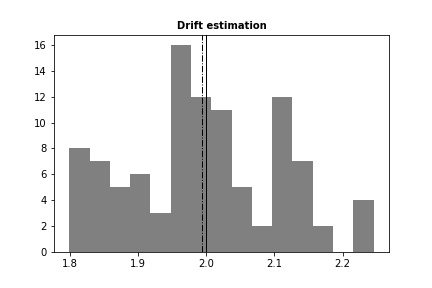
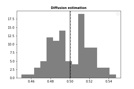
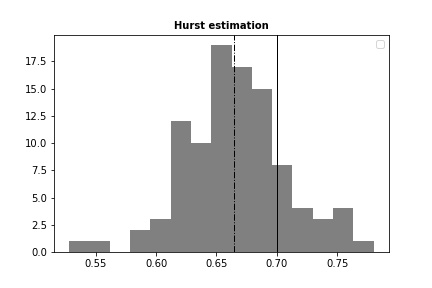
Figure 1: Histograms for the estimation of each parameter separately. The dashed vertical line represents the empirical mean of the estimators and the filled vertical line the true parameters. Left: estimation of $\xi$, the empirical variance is $\sim 10^{-2}$. Right: estimation of $\sigma$, the empirical variance is $\sim 10^{-4}$. Bottom: estimation of $H$, the empirical variance is $\sim 10^{-3}$.

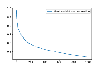
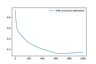
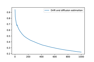
Figure 2: Evolution of the loss function with respect to the number of iterations in the gradient descent. The size of the sample is fixed to $10000$. The true parameters are $\xi=2,\ \sigma=0.5,\ H=0.7$. Left: the estimated parameters are $\sigma=0.57,\ H=0.67$. Right: the estimated parameters are $\xi=1.82,\ H=0.72$. Bottom: the estimated parameters are $\xi=1.83,\ \sigma=0.53$.

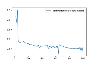
Figure 3: The evolution of the loss function with respect to the number of iterations in the gradient descent, the size of the sample is fixed to $10000$. The true parameters are $\xi=2,\ \sigma=0.5,\ H=0.7$. The estimated parameters are $\xi=1.57,\ \sigma=0.43,\ H=0.81$.

Discussion.

In the one-dimensional case, we get accurate estimators of the parameters (see Figure 1). When estimating $\xi$, $\sigma$ or $H$, the bias and the variance of the estimator are always of order $10^{-2}$ or less. In the two-dimensional case (Figure 2), we used a mini-batch procedure to reduce the randomness of the algorithm. That is, in equation (5.20), we replace the random simulated term $\Lambda(\theta_{n},\Phi_{n+1})$ by an average over $m=100$ simulations. The results displayed in Figure 2 show the convergence of the estimate to the true parameter $\theta$. We decided to stop the algorithm after $1000$ iterations since the gradient gets flat around the true parameter. We also noticed that the partial derivatives $\Lambda(\theta,\Phi)^{i}$ have different magnitudes and decided to adapt our steps $\eta_{n}$ accordingly.

In the three-dimensional case (Figure 3), the gradient gets flat very soon and the algorithm moves very slowly after a few iterations. Here, we stopped the algorithm after $100$ iterations as the three-dimensional case is quite expensive in terms of numerical complexity.

In general, further exploration and in-depth analysis would be necessary to enhance the integration of our statistical procedure with gradient descent algorithms. This aspect remains open for future investigation.

Beyond the fractional O-U model.

When the stationary distribution is unknown, one can approximate $\mu_{\theta}(f_{\Phi})$ in (5.19) by $\frac{1}{N}\sum_{k=0}^{N-1}f(X^{\theta,\gamma}_{k\bar{\gamma}})$ for some large $N$ and small $\bar{\gamma}$ as we explained in Section 4. In this case, we can write the gradient $\Lambda$ as in [22, Eq (7.6)]:

$$\begin{split}\Lambda(\theta,\phi)&=2(\mu_{\theta}-\mu)\,\cos(\langle\phi,.\rangle)\,\rho_{\theta}(-\sin\langle\phi,.\rangle)\\ &\quad+2(\mu_{\theta}-\mu)\,\sin(\langle\phi,.\rangle)\,\rho_{\theta}(\cos\langle\phi,.\rangle),\end{split}$$ (5.21)

where for any function $g:\mathbb{R}\rightarrow\mathbb{R}$, each component of $\rho_{\theta}(g(\langle\phi,.\rangle))$ reads:

$$\rho_{\theta}(g(\langle\phi,.\rangle))^{i}=\frac{1}{N}g(\langle\phi,X^{\theta,\gamma}_{k\bar{\gamma}}\rangle)\langle\phi,\partial_{\theta^{i}}X^{\theta,\gamma}_{k\bar{\gamma}}\rangle.$$

Therefore, the question is how to simulate paths of the process $\partial_{\theta^{i}}X^{\theta,\gamma}_{\cdot}$. In [22] the authors handle the case when $\theta^{i}$ is the drift parameter $\xi$ and explain how the process can be simulated recursively as

$$\partial_{\xi}U_{(k+1)\bar{\gamma}}^{\theta,\gamma}=\partial_{\xi}U_{k\bar{\gamma}}^{\theta,\gamma}+\bar{\gamma}\left(\partial_{\xi}b_{\xi}(U_{k\bar{\gamma}}^{\theta,\gamma})+\nabla b_{\xi}(U_{k\bar{\gamma}}^{\theta,\gamma})\partial_{\xi}U_{k\bar{\gamma}}^{\theta,\gamma}\right).$$

The same technique can be used when $\theta^{i}$ is the diffusion parameter $\sigma$:

$$\partial_{\sigma}U_{(k+1)\bar{\gamma}}^{\theta,\gamma}=\partial_{\sigma}U_{k\bar{\gamma}}^{\theta,\gamma}+\bar{\gamma}\nabla b_{\xi}(U_{k\bar{\gamma}}^{\theta,\gamma})\partial_{\sigma}U_{k\bar{\gamma}}^{\theta,\gamma}+\left(B_{(k+1)\bar{\gamma}}-B_{k\bar{\gamma}}\right).$$

Finally, in order to compute $(\partial_{H}U_{k\gamma})_{k=0,\dots,N}$ in the same way, one needs to compute $\partial_{H}B_{\cdot}$, which is not an obvious task. For instance, using the Mandelbrot-Van Ness representation (2.3), one cannot simply differentiate the integrand with respect to $H$ to get $\partial_{H}B_{\cdot}$. In [20], it is shown that for all $t\geq 0$, $B_{t}$ is almost surely infinitely differentiable with respect to $H$. But since we consider ergodic increments, we need a result that states: almost surely, for all $t\geq 0$, $B_{t}$ is infinitely differentiable with respect to $H$. So maybe in this case, one should look into derivative-free methods for optimization (e.g [8]), where one can perform a gradient descent without having to compute the gradient. This opens new potential problems when considering models beyond the fractional Ornstein-Uhlenbeck, which we leave for future investigation.

Appendix A Regularity in the Hurst parameter

In this section, we recall and adapt some results from our companion paper [14, Sections 4 and 5] that state the regularity in the Hurst parameter of continuous and discrete ergodic means. Recall that the fractional OU process is defined by (5.3), and let us denote by $\bar{U}^{(1,\sigma,H)}$ the stationary fractional OU process with drift $\xi=1$, diffusion matrix $\sigma$ and Hurst parameter $H$.

In the whole Appendix, let $\mathcal{H}$ be a compact subset of $(0,1)$, $\Xi$ be a compact subset of $\mathbb{R}^{m}$, $\Sigma$ a compact subset of the space of $d\times d$ invertible matrices and denote $\Theta=\Xi\times\Sigma\times\mathcal{H}$.

Lemma A.1.

Let $\varpi\in\left(0,1\right)$ and $p\geq 1$. Let $W$ be an $\mathbb{R}^{d}$-Brownian motion and for any $H\in(0,1)$, denote by $B^{H}$ the fBm with underlying noise $W$ (i.e. as in (2.3)). There exists a random variable $\mathbf{C}$ with a finite moment of order $p$ such that almost surely, for any $t\geq 0$, any $\theta_{1}=(\xi,\sigma,H_{1})\in\Theta$ and $\theta_{2}=(\xi,\sigma,H_{2})\in\Theta$,

$$\frac{1}{t+1}\int_{0}^{t+1}\left|Y_{s}^{\theta_{1}}-Y_{s}^{\theta_{2}}\right|^{2}ds\leq\mathbf{C}|H_{1}-H_{2}|^{\varpi},$$

where $Y^{\theta_{1}}$ (resp. $Y^{\theta_{2}}$) is the solution to (2.6) with parameter $\theta_{1}$ (resp. $\theta_{2}$), a drift $b_{\xi}$ satisfying $\mathbf{A_{1}}$. and driving fBm $B^{H_{1}}$ (resp. $B^{H_{2}}$), and $Y^{\theta_{1}}$ and $Y^{\theta_{2}}$ start from the same initial condition.

Proof.

For $i=1,2$, the process $\sigma^{-1}Y_{\cdot}^{\theta_{i}}$ is solution to the SDE

$$\sigma^{-1}Y_{t}^{\theta_{i}}=\sigma^{-1}Y_{0}+\int_{0}^{t}\tilde{b}_{\xi}(\sigma^{-1}Y_{s}^{\theta_{i}})ds+B^{H_{i}}_{t},$$

with $\tilde{b}_{\xi}(x)=\sigma^{-1}b_{\xi}(\sigma\cdot)$. We have $\tilde{b}_{\xi}\in\mathcal{C}^{1,1}(\mathbb{R}^{d}\times\Xi,\mathbb{R}^{d})$ and since $\sigma$ lives in the compact set $\Sigma$, $\tilde{b}_{\xi}$ still satisfies (2.4) and (2.5). We choose the stationary fOU $\bar{U}^{(1,\operatorname{Id},H_{1})}$ with the same noise $B^{H_{1}}$ as $Y^{\theta_{1}}$ (similarly for $\bar{U}_{s}^{(1,\operatorname{Id},H_{2})}$). As in the proof of [14, Theorem 4.5], a comparison between $Y_{s}^{\theta_{1}}-Y_{s}^{\theta_{2}}$ and $\bar{U}^{(1,\operatorname{Id},H_{1})}-\bar{U}^{(1,\operatorname{Id},H_{2})}$ gives

$$\frac{1}{t+1}\int_{0}^{t+1}\left|\sigma^{-1}(Y_{s}^{\theta_{1}}-Y_{s}^{\theta_{2}})\right|^{2}ds \leq C|\bar{U}_{0}^{(1,\operatorname{Id},H_{1})}-\bar{U}_{0}^{(1,\operatorname{Id},H_{2})}|^{2}$$

$$\quad+\frac{1}{t+1}\int_{0}^{t+1}|\bar{U}_{s}^{(1,\operatorname{Id},H_{1})}-\bar{U}_{s}^{(1,\operatorname{Id},H_{2})}|^{2}ds.$$

We can now apply [14, Proposition 4.2] with $t^{\prime}=t=0$ and [14, Proposition 4.4] with $H^{\prime}=K=K^{\prime}$ and $t^{\prime}=t$ to get that there exists a random variable $\mathbf{C}_{1}$ (independent of $\xi$ and $\sigma$) with a finite moment of order $p$ such that

$$\frac{1}{t+1}\int_{0}^{t+1}\left|\sigma^{-1}(Y_{s}^{\theta_{1}}-Y_{s}^{\theta_{2}})\right|^{2}ds\leq\mathbf{C}_{1}|H_{1}-H_{2}|^{\varpi}.$$

Since $\left|\sigma^{-1}(Y_{s}^{\theta_{1}}-Y_{s}^{\theta_{2}})\right|\geq|\sigma^{-1}|\left|(Y_{s}^{\theta_{1}}-Y_{s}^{\theta_{2}})\right|$, dividing by $|\sigma^{-1}|$ and taking the supremum over $\Sigma$, we get the desired result by setting $\mathbf{C}=|\sigma^{-1}|^{-1}\mathbf{C}_{1}$. ∎

Lemma A.2.

Let $\mathcal{H}$ be a compact subset of $\left(0,1\right)$, $\varpi\in\left(0,1\right)$, and $p\geq 1$. There exists $\gamma_{0}>0$ such that for $\gamma\in\left(0,\gamma_{0}\right)$, there exists a random variable $\mathbf{C}_{\gamma}$ with a finite moment of order $p$ such that almost surely, for all $t,t^{\prime}\geq 0$ and all $H_{1},H_{2}\in\mathcal{H}$,

$$\frac{1}{t+1}\int_{0}^{t+1}|\bar{U}_{s_{\gamma}}^{(1,\operatorname{Id},H_{1})}-\bar{U}_{s_{\gamma}}^{(1,\operatorname{Id},H_{2})}|^{2}ds\leq\mathbf{C}_{\gamma}|H_{1}-H_{2}|^{\varpi},$$

where $s_{\gamma}$ denotes the leftmost point in a time-discretisation of step $\gamma$.

Proof.

Apply [14, Proposition 5.1], with $t^{\prime}=t$ and $H^{\prime}=K^{\prime}=K$ to get that

$$\frac{1}{t+1}\int_{0}^{t+1}|\bar{U}_{s_{\gamma}}^{(1,\operatorname{Id},H_{1})}-\bar{U}_{s_{\gamma}}^{(1,\operatorname{Id},H_{2})}|^{2}ds\leq\mathbf{C}_{\gamma}|H_{1}-H_{2}|^{\varpi}+C\mathbb{E}|\bar{U}_{0}^{(1,\operatorname{Id},H_{1})}-\bar{U}_{0}^{(1,\operatorname{Id},H_{2})}|^{2}.$$

Now apply [14, Proposition 4.2] with $t=t^{\prime}=0$ to get the desired result. ∎

Lemma A.3.

Let $\mathcal{H}$ be a compact subset of $\left(0,1\right)$. Let $\varpi\in\left(0,1\right)$ and $p\geq 1$. There exists $\gamma_{0}>0$ such that for $\gamma\in\left(0,\gamma_{0}\right]$, there exists a random variable $\mathbf{C}_{\gamma}$ with a finite moment of order $p$ such that almost surely, for any $N\in\mathbb{N}^{*}$, any $\theta=(\xi,\sigma,H_{1})$ and any $\theta_{2}=(\xi,\sigma,H_{2})\in\Theta$,

$$\frac{1}{N}\sum_{k=1}^{N}\left|Y_{k\gamma}^{\theta_{1},\gamma}-Y_{k\gamma}^{\theta_{2},\gamma}\right|^{2}\leq\mathbf{C}_{\gamma}|H_{1}-H_{2}|^{\varpi},$$

where $Y^{\theta_{2},\gamma}$ and $Y^{\theta_{2},\gamma}$ are Euler schemes (4.1) with the same initial condition and driven by fBm with the same underlying noise (see (2.3)).

Proof.

For any $\theta\in\Theta$, the process $\sigma^{-1}Y_{\cdot}^{\theta,\gamma}$ is solution to the SDE

$$\sigma^{-1}Y_{t}^{\theta,\gamma}=\sigma^{-1}Y_{0}+\int_{0}^{t}\tilde{b}_{\xi}(\sigma^{-1}Y_{s_{\gamma}}^{\theta,\gamma})ds+B_{t}^{H},$$

with $\tilde{b}_{\xi}(x)=\sigma^{-1}b_{\xi}(\sigma\cdot)$. We have $\tilde{b}_{\xi}\in\mathcal{C}^{1,1}(\mathbb{R}^{d}\times\Xi,\mathbb{R}^{d})$ and since $\sigma$ lives in the compact set $\Sigma$, one can check that $\tilde{b}_{\xi}$ still satisfies (2.4) and (2.5). As in the proof of [14, Eq. (5.5)], a comparison with the stationary fOU process $\bar{U}$ gives

$$\frac{1}{N}\sum_{k=0}^{N}\left|\sigma^{-1}(Y_{k\gamma}^{\theta_{1},\gamma}-Y_{k\gamma}^{\theta_{2},\gamma})\right|^{2} \leq C\Bigg{(}\frac{1}{N}\sum_{k=0}^{N}\left|\bar{U}_{j\gamma}^{(1,\operatorname{Id},H_{1})}-\bar{U}_{j\gamma}^{(1,\operatorname{Id},H_{2})}\right|^{2}$$

$$\quad+\left|\bar{U}_{0}^{(1,\operatorname{Id},H_{1})}-\bar{U}_{0}^{(1,\operatorname{Id},H_{2})}\right|^{2}+\frac{1}{N\gamma}\int_{0}^{N\gamma}\left|U_{s}^{(1,\operatorname{Id},H_{1})}-U_{s}^{(1,\operatorname{Id},H_{2})}\right|^{2}ds\Bigg{)}.$$

The regularity of the second term in the right-hand side is given by [14, Proposition 4.2] and the regularity of the third term is given by [14, Theorem 4.5]. To bound the first term, we apply Lemma A.2. To conclude the proof, we notice that $|\sigma^{-1}(Y_{k\gamma}^{\theta_{1},\gamma}-Y_{k\gamma}^{\theta_{2},\gamma})|\geq|\sigma^{-1}||(Y_{k\gamma}^{\theta_{1}}-Y_{k\gamma}^{\theta_{2}})|$, divide by $|\sigma^{-1}|$ and take the supremum over $\Sigma$. ∎

Appendix B Continuity and Tightness results

In Proposition B.1 and Proposition B.2, we prove that the solutions $Y^{\theta}$ and $Y^{\theta,\gamma}$ to (2.6) and (4.1) and their ergodic means have finite moments uniformly in time and $\theta$. Finally, in Proposition B.3, we state a result on the the regularity of the ergodic means in $\theta$.

Proposition B.1.

Assume $\mathbf{A_{0}}$. and $\mathbf{A_{1}}$.. Let $Y^{\theta}$ be the unique solution of (2.6). Let $p>1$. Then the following inequalities hold true:

• $\displaystyle\sup_{t\geq 0}\sup_{\theta\in\Theta}\mathbb{E}|Y_{t}^{\theta}|^{p}<\infty$.

• $\displaystyle\mathbb{E}\left(\sup_{t\geq 0}\sup_{\theta\in\Theta}\frac{1}{t}\int_{0}^{t}|Y_{s}^{\theta}|^{2}ds\right)^{p}<\infty$.

• $\displaystyle\mathbb{E}\left(\sup_{t\geq 0}\sup_{\theta\in\Theta}\frac{1}{n}\sum_{k=0}^{n-1}|Y_{kh}^{\theta}|^{2}\right)^{p}<\infty$.

Proof.

Throughout the proof, $C$ will denote a constant that do not depend on $\theta$ or $t$ and that may change from line to line. Observe that when the supremum is taken only over $\xi$, the proof is already done in [22, Proposition A.1]. The proofs of all three items are based on a comparison with fractional OU processes defined in (5.3).

For the proof of $(i)$, by [12, p 725], a comparison with the stationary fractional OU process $U^{(1,\sigma,H)}$ yields that there exist constants $c_{1},c_{2}>0$ independent of $\xi$ such that,

$$|Y_{t}-\bar{U}_{t}^{(1,\sigma,H)}|^{p}\leq e^{-2c_{1}t}|Y_{0}|^{p}+c_{2}\int_{0}^{t}e^{-2c_{2}(t-s)}(1+|\bar{U}_{s}^{(1,\sigma,H)}|^{p})ds.$$

Moreover, since $U^{(1,\sigma,H)}$ is a Gaussian process, for any $t\geq 1$, we have $\mathbb{E}|\bar{U}_{t}^{(1,\sigma,H)}|^{p}\lesssim(\mathbb{E}|\bar{U}_{t}^{(1,\sigma,H)}|^{2})^{p/2}$. By (5.5), we know that $\mathbb{E}|\bar{U}_{t}^{(1,\sigma,H)}|^{2}=\sigma^{2}H\Gamma(2H)$. Therefore

$$\sup_{t\geq 0}\sup_{\theta\in\Theta}\mathbb{E}|Y_{t}^{\theta}|^{p}\leq C(1+\sup_{t\geq 0}\sup_{\theta\in\Theta}\mathbb{E}|\bar{U}_{t}^{(1,\sigma,H)}|^{p})<\infty.$$

For the proof of $(ii)$, we follow the steps of the proof of Proposition A.1 in [22] (see equation (A.6) and what follows), to get that for all $t>0$,

$$\sup_{\theta\in\Theta}\frac{1}{t}\int_{0}^{t}|Y_{s}^{\theta}|^{2}ds \leq C\sup_{\theta\in\Theta}\frac{1}{t}\int_{0}^{t}|U_{s}^{\theta}|^{2}ds\leq C\sup_{\theta=(1,\sigma,H)\in\Theta}\frac{1}{t}\int_{0}^{t}|\sigma||U_{s}^{(1,\operatorname{Id},H)}|^{2}ds.$$

It follows that

$$\sup_{\theta\in\Theta}\frac{1}{t}\int_{0}^{t}|Y_{s}^{\theta}|^{2}ds \leq C\sup_{H\in\mathcal{H}}\frac{1}{t}\int_{0}^{t}|U_{s}^{(1,\operatorname{Id},H)}|^{2}ds$$

$$\leq C\Biggl{(}\sup_{H\in\mathcal{H}}\frac{1}{t}\int_{0}^{t}|U_{s}^{(1,\operatorname{Id},H)}-U_{s}^{(1,\operatorname{Id},1/2)}|^{2}ds+\frac{1}{t}\int_{0}^{t}|U_{s}^{(1,\operatorname{Id},1/2)}|^{2}ds\Biggr{)}.$$

Moreover, by Lemma A.1 applied to $Y^{\theta}\equiv U^{(1,\operatorname{Id},H)}$ we have that for any $\varpi\in(0,1)$, there exists a random variable $\mathbf{C}$ with a finite moment of order $p$ such that for any $t\geq 1$,

$$\frac{1}{t}\int_{0}^{t}\sup_{\theta\in\Theta}|Y_{s}^{\theta}|^{2}ds \leq C\Biggl{(}\mathbf{C}\sup_{H\in\mathcal{H}}|H-\frac{1}{2}|^{\varpi}+\frac{1}{t}\int_{0}^{t}|U_{s}^{(1,\operatorname{Id},1/2)}|^{2}ds\Biggr{)}.$$

The ergodicity of $U^{(1,\operatorname{Id},1/2)}$ implies that $\frac{1}{t}\int_{0}^{t}|U_{s}^{(1,\operatorname{Id},1/2)}|^{2}ds$ converges as $t\to\infty$. It follows that

$$\mathbb{E}\left(\sup_{t>0}\sup_{\theta\in\Theta}\frac{1}{t}\int_{0}^{t}|Y_{s}^{\theta}|^{2}ds\right)^{p}<\infty.$$

The proof of $(iii)$ can be done in the exact same way by transcribing all the integrals to discrete sums and using Lemma A.2. ∎

Proposition B.2.

Assume $\mathbf{A_{0}}$. and $\mathbf{A_{1}}$.. Let $Y_{\cdot}^{\theta,\gamma}$ be the Euler scheme (4.1). Then there exists $\gamma_{0}>0$ such that for any $p>1$, there is

• $\displaystyle\sup_{\theta\in\Theta,\gamma\in(0,\gamma_{0})}\limsup_{N\rightarrow\infty}\mathbb{E}\left|Y^{\theta,\gamma}_{N\gamma}\right|^{p}<\infty$.

• For $\gamma\in(0,\gamma_{0}]$, $\displaystyle\mathbb{E}\left(\sup_{\theta\in\Theta}\sup_{N\geq 1}\frac{1}{N}\sum_{k=0}^{N-1}|Y^{\theta,\gamma}_{k\gamma}|^{2}\right)^{p}<\infty$.

Proof.

Note that the same results are proven in [22, Proposition A.4] when $\Theta$ only represents the range of the parameter $\xi$. With this in mind, as in Proposition B.1, the proof of $(i)$ is based on comparisons with the discrete Ornstein-Uhlenbeck process, which has finite moments uniformly in $\theta$. The proof $(ii)$ is the same as the proof of $(ii)$ in Proposition B.1 and is based on a comparison with the discrete OU process and Lemma A.3. ∎

Proposition B.3.

Let the assumptions $\mathbf{A_{0}}$. and $\mathbf{A_{1}}$. hold. Assume also that the exponent $r$ in the sub-linear growth of $b_{\xi}$ in (2.5) satisfies $r\leq 1$. Let $p\geq 1$ and $\varpi\in(0,1)$, then there exists a positive random variable $\mathbf{C}$ that has a finite moment of order $p$, such that almost surely for all $\theta_{1},\theta_{2}\in\Theta$ and for all $t\geq 1$,

$$\frac{1}{t}\int_{0}^{t}|Y_{s}^{\theta_{1}}-Y_{s}^{\theta_{2}}|^{2}ds\leq\mathbf{C}|\theta_{1}-\theta_{2}|^{\varpi},$$ (B.1)

where $Y^{\theta_{1}}$ and $Y^{\theta_{2}}$ are solutions to (2.6) with the same initial condition and driven by an fBm with the same underlying noise (see (2.3)). Furthermore, there exists $\gamma_{0}$ such that for any $\gamma\in(0,\gamma_{0}]$, there exists a positive random variable $\mathbf{C}_{\gamma}$ that has a finite moment of order $p$, such that almost surely, for any $\theta_{1},\theta_{2}\in\Theta$ and any $N\geq 1$,

$$\frac{1}{N}\sum_{k=0}^{N}|Y_{k\gamma}^{\theta_{1},\gamma}-Y_{k\gamma}^{\theta_{2},\gamma}|^{2}ds\leq\mathbf{C}_{\gamma}|\theta_{1}-\theta_{2}|^{\varpi}.$$ (B.2)

Proof.

In the proof, we denote by $C$ a constant independent of time and $\theta$ that may change from line to line. Similarly, $\mathbf{C}$ will denote a positive random variable that has a finite moment of order $p$, that does not depend on $\theta$ and may change from line to line. Let us first focus on on the proof of (B.1). Up to introducing pivot terms, we can consider three different cases:

$$\text{1)}~{}\theta_{1} =(\xi_{1},\sigma,H),\theta_{2}=(\xi_{2},\sigma,H)$$

$$\text{2)}~{}\theta_{1} =(\xi,\sigma,H_{1}),~{}\theta_{2}=(\xi,\sigma,H_{2})$$

$$\text{3)}~{}\theta_{1} =(\xi,\sigma_{1},H),~{}\theta_{2}=(\xi,\sigma_{2},H).$$

In the first case, we have by [22, Eq. (5.32)] that

$$\frac{1}{t}\int_{0}^{t}|Y_{s}^{\theta_{1}}-Y_{s}^{\theta_{2}}|^{2}ds\leq C|\xi_{1}-\xi_{2}|^{2}\left(1+\sup_{\theta\in\Theta}\frac{1}{t}\int_{0}^{t}|Y_{s}^{\theta}|^{2r}ds\right),$$

where $r$ is the exponent in the sub-linear growth assumption on $b_{\xi}$. Since $r\leq 1$, we have

$$\frac{1}{t}\int_{0}^{t}|Y_{s}^{\theta_{1}}-Y_{s}^{\theta_{2}}|^{2}ds\leq C|\xi_{1}-\xi_{2}|^{2}\left(1+\sup_{\theta\in\Theta}\frac{1}{t}\int_{0}^{t}|Y_{s}^{\theta}|^{2}ds\right).$$ (B.3)

It follows from the uniform bound on the moments of $Y_{t}^{\theta}$ in Proposition B.1(ii) that there exists a random variable $\mathbf{C}$ with finite moment of order $p$ such that

$$\frac{1}{t}\int_{0}^{t}|Y_{s}^{\theta_{1}}-Y_{s}^{\theta_{2}}|^{2}ds\leq\mathbf{C}|\xi_{1}-\xi_{2}|^{2}.$$

The second case is directly the result of Lemma A.1.

As for the third case, the idea is to compare the process $Y$ with the fractional OU processes $U^{(1,\sigma_{1},H)}$ and $U^{(1,\sigma_{2},H)}$ defined by (5.3) with the same initial condition and the same driving fBm. For $s\geq 1$, we have

$$\frac{\partial}{\partial s}|Y_{s}^{\theta_{1}}-Y_{s}^{\theta_{2}}-\left(U_{s}^{(1,\sigma_{1},H)}-U_{s}^{(1,\sigma_{2},H)}\right)|^{2}$$

$$\quad=2\langle Y_{s}^{\theta_{1}}-Y_{s}^{\theta_{2}}-\left(U_{s}^{(1,\sigma_{1},H)}-U_{s}^{(1,\sigma_{2},H)}\right),b(Y_{s}^{\theta_{1}})-b(Y_{s}^{\theta_{2}})+\left(U_{s}^{(1,\sigma_{1},H)}-U_{s}^{(1,\sigma_{2},H)}\right)\rangle$$

$$\quad\leq-c_{1}|Y_{s}^{\theta_{1}}-Y_{s}^{\theta_{2}}|^{2}-c_{2}|U_{s}^{(1,\sigma_{1},H)}-U_{s}^{(1,\sigma_{2},H)}|^{2}+c_{3}|Y_{s}^{\theta_{1}}-Y_{s}^{\theta_{2}}||U_{s}^{(1,\sigma_{1},H)}-U_{s}^{(1,\sigma_{2},H)}|,$$

where the last inequality follows from $\mathbf{A_{1}}$.. Next, we apply Young’s inequality to get

$$\frac{\partial}{\partial s}|Y_{s}^{\theta_{1}}-Y_{s}^{\theta_{2}}-\left(U_{s}^{(1,\sigma_{1},H)}-U_{s}^{(1,\sigma_{2},H)}\right)|^{2}$$

$$\quad\leq-c_{1}|Y_{s}^{\theta_{1}}-Y_{s}^{\theta_{2}}|^{2}-c_{2}|U_{s}^{(1,\sigma_{1},H)}-U_{s}^{(1,\sigma_{2},H)}|^{2}+c_{3}|U_{s}^{(1,\sigma_{1},H)}-U_{s}^{(1,\sigma_{2},H)}|^{2}$$

$$\quad\leq-c_{1}|Y_{s}^{\theta_{1}}-Y_{s}^{\theta_{2}}-\left(U_{s}^{(1,\sigma_{1},H)}-U_{s}^{(1,\sigma_{2},H)}\right)|^{2}+c_{2}|U_{s}^{(1,\sigma_{1},H)}-U_{s}^{(1,\sigma_{2},H)}|^{2}.$$

We can now apply Grönwall’s lemma to get

$$|Y_{s}^{\theta_{1}}-Y_{s}^{\theta_{2}}-\left(U_{s}^{(1,\sigma_{1},H)}-U_{s}^{(1,\sigma_{2},H)}\right)|^{2}\leq C\int_{0}^{s}e^{-(s-u)}|U_{u}^{(1,\sigma_{1},H)}-U_{u}^{(1,\sigma_{2},H)}|^{2}du.$$

Jensen’s inequality yields that

$$|Y_{s}^{\theta_{1}}-Y_{s}^{\theta_{2}}-\left(U_{s}^{(1,\sigma_{1},H)}-U_{s}^{(1,\sigma_{2},H)}\right)|^{2}\leq C\int_{0}^{s}e^{-(s-u)}|U_{u}^{(1,\sigma_{1},H)}-U_{u}^{(1,\sigma_{2},H)}|^{2}du,$$

and therefore

$$|Y_{s}^{\theta_{1}}-Y_{s}^{\theta_{2}}|^{2}\leq C\Bigg{(}|U_{s}^{(1,\sigma_{1},H)}-U_{s}^{(1,\sigma_{2},H)}|^{2}+\int_{0}^{s}e^{-(s-u)}|U_{u}^{(1,\sigma_{1},H)}-U_{u}^{(1,\sigma_{2},H)}|^{2}du\Bigg{)}.$$

Then, using Fubini’s theorem, it comes that

$$\frac{1}{t}\int_{0}^{t}|Y_{s}^{\theta_{1}}-Y_{s}^{\theta_{2}}|^{2}ds \leq\frac{C}{t}\int_{0}^{t}|U_{u}^{(1,\sigma_{1},H)}-U_{u}^{(1,\sigma_{2},H)}|^{2}\int_{u}^{t}\mathds{1}_{[0,s]}e^{-(s-u)}dsdu$$

$$\quad+\frac{C}{t}\int_{0}^{t}|U_{s}^{(1,\sigma_{1},H)}-U_{s}^{(1,\sigma_{2},H)}|^{2}ds$$

$$\leq\frac{C}{t}\int_{0}^{t}|U_{u}^{(1,\sigma_{1},H)}-U_{u}^{(1,\sigma_{2},H)}|^{2}du.$$ (B.4)

Now, observe that

$$U_{s}^{(1,\sigma_{1},H)}-U_{s}^{(1,\sigma_{2},H)}=(\sigma_{1}-\sigma_{2})U_{s}^{(1,\operatorname{Id},H)}.$$

Since $U_{s}^{(1,\operatorname{Id},H)}$ has finite moments uniformly in $\theta$ (recall (5.5) and that $U^{(1,\operatorname{Id},H)}$ is a Gaussian process), it follows that

$$\frac{1}{t}\int_{0}^{t}|Y_{s}^{\theta_{1}}-Y_{s}^{\theta_{2}}|^{2}ds\leq\mathbf{C}|\sigma_{1}-\sigma_{2}|^{2},$$

where $\mathbf{C}$ has a finite moment of order $p$. This concludes the proof of (B.1).

The proof of (B.2) is obtained using discrete analogues of the previous arguments. More precisely, in the first case, similarly to (B.3), we have from [22, Proposition 3.8 (ii)] that

$$\frac{1}{N}\sum_{k=0}^{N}|Y_{k\gamma}^{\theta_{1},\gamma}-Y_{k\gamma}^{\theta_{2},\gamma}|^{2}\leq C|\xi_{1}-\xi_{2}|^{2}\left(1+\sup_{\theta\in\Theta}\frac{1}{N}\sum_{k=0}^{N}|Y_{k\gamma}^{\theta,\gamma}|^{2}\right).$$

Note that while the dependence of the right-hand side on $\sigma$ and $H$ in [22] is not explicit, one can show that the upper bound they obtain in the continuous setting (i.e [22, Eq. (5.32)]) still holds if the integrals are replaced by discrete sums. Then, using the uniform bound on the moments of $Y^{\theta,\gamma}$ in Proposition B.2 (ii), we conclude.

The second case is directly the result of Lemma A.3. In the third case, similarly to (B.4), via a comparison with the discrete fOU process $U^{\theta,\gamma}$ (that solves (4.1) with $b_{\xi}(\cdot)=-\xi\cdot$), one can show that

$$\frac{1}{N}\sum_{k=0}^{N}|Y_{k\gamma}^{\theta_{1},\gamma}-Y_{k\gamma}^{\theta_{2},\gamma}|^{2} \leq\frac{C}{N}\sum_{k=0}^{N}|U_{k\gamma}^{(1,\sigma_{1},H),\gamma}-U_{k\gamma}^{(1,\sigma_{2},H),\gamma}|^{2}.$$

Then we use the linearity of $U^{(1,\sigma,H),\gamma}$ in $\sigma$ to conclude. ∎

Appendix C Proof of Proposition 4.1

The proof follows the same steps as the proof of Lemma 2.2. Let $\theta=(\xi,\sigma,H)\in\Theta$. We will first prove that almost surely, the random measure $\frac{1}{t}\int_{0}^{t}\delta_{X^{\theta,\gamma}_{s}}ds$ converges in law to $\mu_{\theta}^{\gamma}$ as $t\rightarrow\infty$. This implies that $\frac{1}{t}\int_{0}^{t}\delta_{X^{\theta,\gamma}_{s}}ds$ converges to $\mu_{\theta}$ in the Prokhorov distance. To extend this result to distances $d$ in $\mathcal{D}_{2}$ (i.e dominated by the $2$-Wasserstein distance), we use the fact that the $2$-Wasserstein distance is dominated by the Prokorov distance $d_{P}$ as follows (see [9, Theorem 2]):

$$d\left(\frac{1}{t}\int_{0}^{t}\delta_{X^{\theta,\gamma}_{s}}ds,\mu_{\theta}\right)\leq C_{p}\sup_{t\geq 0}\left(\max\left(\frac{1}{t}\int_{0}^{t}|X^{\theta,\gamma}_{s}|^{2}ds,\,\mathbb{E}|\bar{X}^{\theta,\gamma}_{t}|^{2}\right)+1\right)d_{P}\left(\frac{1}{t}\int_{0}^{t}\delta_{X^{\theta,\gamma}_{s}}ds,\mu_{\theta}\right).$$

By definition of the process $X^{\theta,\gamma}$, we have that

$$\max\left(\frac{1}{t}\int_{0}^{t}|X^{\theta,\gamma}_{s}|^{2}ds,\,\mathbb{E}|\bar{X}^{\theta,\gamma}_{t}|^{2}\right)\leq C_{q}\sum_{i=0}^{q}\max\left(\frac{1}{t}\int_{0}^{t}|Y^{\theta,\gamma}_{s+ih}|^{2}ds,\,\mathbb{E}|\bar{Y}^{\theta,\gamma}_{s+ih}|^{2}\right).$$

Therefore, we conclude thanks to Proposition B.2 that in the present case, the convergence in law is equivalent to the convergence for the $2$-Wasserstein distance. Similarly to Section 3.2, we consider a family of probability measures on the set of càdlàg functions for which the identification of the limit will be easier, namely $\{\pi_{N}=\frac{1}{N}\sum_{k=0}^{N-1}\delta_{X_{k\gamma+.}^{\theta,\gamma}}\}_{N\geq 0}$. We first prove that the family is tight and then identify the limit as the stationary law of the augmented process $\bar{X}^{\theta,\gamma}$. Tightness in $D(\mathbb{R}_{+},\mathbb{R}^{d})$, the space of functions that are right-continuous and have limits from the left is equivalent to tightness in $D([0,T],\mathbb{R}^{d})$ for every $T>0$. Thus by [3, Theorem 13.2], tightness is equivalent to the following two points that must hold for any $T>0$:

1. $\displaystyle\lim_{a\rightarrow\infty}\limsup_{N\rightarrow\infty}\pi_{N}\left(x:\sup_{t\in[0,T]}|x_{t}|\geq a\right)=0.$

2. For any $\eta>0$,

   $$\limsup_{\delta\rightarrow 0}\limsup_{N\rightarrow+\infty}\pi_{N}\left(x:w_{T}^{\prime}(x,\delta)\geq\eta\right)=\limsup_{\delta\rightarrow 0}\limsup_{N\rightarrow+\infty}\frac{1}{N}\sum_{k=0}^{N-1}\mathds{1}_{\left\{w_{T}^{\prime}\left(X^{\theta,\gamma}_{k\gamma+\cdot},\delta\right)\geq\eta\right\}}=0\quad\text{ a.s.}\,,$$

   with

   $$w_{T}^{\prime}(x,\delta)=\inf_{\left\{t_{i}\right\}}\left\{\max_{i\leq r}\sup_{s,t\in\left[t_{i},t_{i+1}\right)}\left|x_{t}-x_{s}\right|\right\},$$

   where the infimum runs over finite sets $\left\{t_{i}\right\}_{i=1,\dots,r},r\in\mathbb{N}^{*}$, satisfying

   $$0=t_{0}<t_{1}<\cdots<t_{r}=T\quad\text{ and }\quad\inf_{i\leq r}\left(t_{i}-t_{i-1}\right)\geq\delta.$$

Since the process has only jumps at times $n\gamma$ with $n\in\mathbb{N}$, $w_{T}^{\prime}\left(X^{\theta,\gamma},\delta\right)=0$ when $\delta<\gamma$, which implies that the second condition (ii) holds.

The first condition (i) is equivalent to tightness in the space of probability measures on $\mathbb{R}$ of the sequence $(\mu_{T}^{N})_{N\in\mathbb{N}^{*}}$ defined by

$$\mu_{T}^{N}=\frac{1}{N}\sum_{k=0}^{N-1}\delta_{\left\{\sup_{t\in[0,T]}\left|X_{k\gamma+t}^{\theta,\gamma}\right|\right\}}.$$

Recall that by definition of $X$ we have $|X^{\theta,\gamma}_{k\gamma}|^{2}\leq C_{q}\sum_{i=0}^{q}|Y^{\theta,\gamma}_{k\gamma+ih}|^{2}\leq C_{q}\sup_{i\in\llbracket 0,q\rrbracket}|Y^{\theta,\gamma}_{k\gamma+ih}|^{2}$. Hence, for $V(x)=|x|^{2}$ and

$$\tilde{\mu}^{N}_{T}=\frac{1}{N}\sum_{k=0}^{N-1}\delta_{\left\{\sup_{t\in[0,T+qh]}\left|Y^{\theta,\gamma}_{k\gamma+t}\right|\right\}},$$

we deduce that

$$\mu_{T}^{N}(V)\leq C_{q}\,\tilde{\mu}^{N}_{T}(V).$$

From the last equation in the proof of [6, Proposition 2], we have $\sup_{N\geq 1}\tilde{\mu}^{N}_{T}(V)<+\infty$ almost surely, which implies that $(\mu_{T}^{N})_{N\geq 1}$ is a.s. tight on $\mathbb{R}$ (see e.g. [7, Proposition 2.1.6]).

Now let $(t_{n})_{n\geq 1}$ be an increasing sequence going to $+\infty$ and $\{\frac{1}{t_{n}}\sum_{k=0}^{t_{n}-1}\delta_{X^{\theta,\gamma}_{k\gamma+\cdot}}\}_{n\geq 1}$ be a (pathwise) sequence with limiting distribution $\rho$. We first show that $\rho$ is the law of a stationary process. Let $M\geq 1$, $(u_{1},\dots,u_{M})\in\mathbb{N}^{M}$ and $f:\mathbb{R}^{M(q+1)}\mapsto\mathbb{R}$, then for all $T\in\mathbb{N}^{*}$,

$$\frac{1}{t_{n}}\sum_{k=0}^{t_{n}-1}\left(f\left(X^{\theta,\gamma}_{u_{1}\gamma+k\gamma+T\gamma},\ldots,X^{\theta,\gamma}_{u_{M}\gamma+k\gamma+T\gamma}\right)\right)-f\left(X^{\theta,\gamma}_{u_{1}+k\gamma},\ldots,X^{\theta,\gamma}_{u_{M}+k\gamma}\right)$$

$$\quad=\frac{1}{t_{n}}\left(\sum_{k=t_{n}}^{t_{n}+T-1}f\left(X^{\theta,\gamma}_{u_{1}+k\gamma},\ldots,X^{\theta,\gamma}_{u_{M}+k\gamma}\right)-\sum_{k=0}^{T-1}f\left(X^{\theta,\gamma}_{u_{1}+k\gamma},\ldots,X^{\theta,\gamma}_{u_{M}+k\gamma}\right)\right).$$

Since $f$ is bounded and both the sums in the last term are over bounded intervals, we deduce that the last term converges a.s. to $0$ when $t_{n}\rightarrow\infty$. Therefore, $\rho$ is the law of a stationary process. Let us now prove that $\rho$ is the law of $\bar{X}^{\theta,\gamma}$.

A process ${x_{t}=(y_{t},z^{1}_{t},\dots,z^{q}_{t})}$ has the law of $\bar{X}^{\theta,\gamma}$ if $x_{t}=x_{k\gamma}$ for $t\in[k\gamma,(k+1)\gamma]$, and

$$y_{\cdot}-y_{0}-\int_{0}^{\cdot_{\gamma}}b_{\xi}(y_{u})du~{}\text{has the law of a $\sigma B_{\cdot_{\gamma}}$ where B has Hurst parameter $H$};$$

$$z^{i}_{\cdot}-\ell^{i}\left(\int_{0}^{\cdot_{\gamma}}b_{\xi}(y_{u})du,\dots,\int_{0}^{(\cdot+ih)_{\gamma}}b_{\xi}(y_{u})du\right)~{}\text{has the law of}~{}\sigma\ell^{i}(B_{\cdot_{\gamma}},\dots,B_{(\cdot+ih)_{\gamma}})~{}\text{for all $i\in\llbracket 1,q\rrbracket$},$$

where for all $t\geq 0$, $t_{\gamma}=\gamma\lfloor t/\gamma\rfloor$. Let us define

$$G_{\gamma}(x_{\cdot})=\begin{pmatrix}y_{\cdot}-y_{0}-\int_{0}^{\cdot_{\gamma}}b_{\xi}(y_{u})du\\ z^{1}_{\cdot}-\ell^{1}\left(\int_{0}^{\cdot_{\gamma}}b_{\xi}(y_{u})du,\int_{0}^{(\cdot+h)_{\gamma}}b_{\xi}(y_{u})du\right)\\ \vdots\\ z^{q}_{\cdot}-\left(\int_{0}^{\cdot_{\gamma}}b_{\xi}(y_{u})du,\dots,\int_{0}^{(\cdot+qh)_{\gamma}}b_{\xi}(y_{u})du\right)\end{pmatrix},$$

and

$$\mathbf{B}_{\cdot} =\left(\sigma B_{\cdot_{\gamma}},\dots,\sigma\ell^{q}(B_{\cdot_{\gamma}},\dots,B_{(\cdot+qh)_{\gamma}})\right).$$

In other words, we have to prove that $\rho\circ G_{\gamma}^{-1}~{}\text{is the law of}~{}\mathbf{B}_{\cdot}$. Since $G_{\gamma}$ is continuous for the u.s.c. topology, we have

$$\gamma\circ G_{\rho}^{-1}=\lim_{n\rightarrow\infty}\frac{1}{t_{n}}\int_{0}^{t_{n}}\delta_{G_{\gamma}(X^{\theta,\gamma}_{s+\cdot})}ds.$$

We omit the rest of the proof as it is almost identical to Section 3.2. That is, for $T>0$ and $F:\mathcal{C}([0,T],\mathbb{R}^{d(q+1)})\mapsto\mathbb{R}$ a bounded measurable function, following the same steps after (3.5), one can show that

$$\lim_{n\rightarrow\infty}\frac{1}{t_{n}}\int_{0}^{t_{n}}F\left(G_{\gamma}(X^{\theta,\gamma}_{s+\cdot})\right)ds=\mathbb{E}F(\mathbf{B}_{\cdot}).$$

Hence, $\rho\circ G_{\gamma}^{-1}$ has the law of $\mathbf{B}$.

References

- [1] Rachid Belfadli, Khalifa Es-Sebaiy, and Youssef Ouknine. Parameter estimation for fractional Ornstein-Uhlenbeck processes: non-ergodic case. Preprint arXiv:1102.5491, 2011.
- [2] Corinne Berzin, Alain Latour, and José R. León. Variance estimator for fractional diffusions with variance and drift depending on time. Electron. J. Stat., 9(1):926–1016, 2015.
- [3] Patrick Billingsley. Convergence of probability measures. Wiley Series in Probability and Statistics: Probability and Statistics. John Wiley & Sons, Inc., New York, second edition, 1999. A Wiley-Interscience Publication.
- [4] Alexandre Brouste and Stefano M. Iacus. Parameter estimation for the discretely observed fractional Ornstein-Uhlenbeck process and the Yuima R package. Comput. Statist., 28(4):1529–1547, 2013.
- [5] Patrick Cheridito, Hideyuki Kawaguchi, and Makoto Maejima. Fractional Ornstein-Uhlenbeck processes. Electron. J. Probab., 8:no. 3, 14, 2003.
- [6] Serge Cohen and Fabien Panloup. Approximation of stationary solutions of Gaussian driven stochastic differential equations. Stochastic Process. Appl., 121(12):2776–2801, 2011.
- [7] Marie Duflo. Random iterative models, volume 34 of Applications of Mathematics (New York). Springer-Verlag, Berlin, 1997. Translated from the 1990 French original by Stephen S. Wilson and revised by the author.
- [8] Abraham D. Flaxman, Adam T. Kalai, and Brendan H. McMahan. Online convex optimization in the bandit setting: gradient descent without a gradient. In Proceedings of the sixteenth annual ACM-SIAM symposium on Discrete algorithms, pages 385–394, 2005.
- [9] Alison L. Gibbs and Francis E. Su. On choosing and bounding probability metrics. International statistical review, 70(3):419–435, 2002.
- [10] Luca M. Giordano, Maria Jolis, and Lluís Quer-Sardanyons. SPDEs with fractional noise in space: continuity in law with respect to the Hurst index. Bernoulli, 26(1):352–386, 2020.
- [11] Arnaud Gloter and Marc Hoffmann. Estimation of the Hurst parameter from discrete noisy data. Ann. Statist., 35(5):1947–1974, 2007.
- [12] Martin Hairer. Ergodicity of stochastic differential equations driven by fractional Brownian motion. Ann. Probab., 33(2):703–758, 2005.
- [13] El Mehdi Haress and Yaozhong Hu. Estimation of all parameters in the fractional Ornstein-Uhlenbeck model under discrete observations. Stat. Inference Stoch. Process., 24(2):327–351, 2021.
- [14] El Mehdi Haress and Alexandre Richard. Long time Hurst regularity of fractional SDEs and their ergodic means. Preprint arXiv:2206.06648, 2022.
- [15] Yaozhong Hu and David Nualart. Parameter estimation for fractional Ornstein-Uhlenbeck processes. Statist. Probab. Lett., 80(11-12):1030–1038, 2010.
- [16] Yaozhong Hu, David Nualart, and Hongjuan Zhou. Parameter estimation for fractional Ornstein-Uhlenbeck processes of general Hurst parameter. Stat. Inference Stoch. Process., 22(1):111–142, 2019.
- [17] Yaozhong Hu and Jian Song. Parameter estimation for fractional Ornstein-Uhlenbeck processes with discrete observations. In Malliavin calculus and stochastic analysis, volume 34 of Springer Proc. Math. Stat., pages 427–442. Springer, New York, 2013.
- [18] Maria Jolis and Noèlia Viles. Continuity with respect to the Hurst parameter of the laws of the multiple fractional integrals. Stochastic Process. Appl., 117(9):1189–1207, 2007.
- [19] Maria Jolis and Noèlia Viles. Continuity in the Hurst parameter of the law of the Wiener integral with respect to the fractional Brownian motion. Statist. Probab. Lett., 80(7-8):566–572, 2010.
- [20] Stefan Koch and Andreas Neuenkirch. The Mandelbrot–Van Ness fractional Brownian motion is infinitely differentiable with respect to its Hurst parameter. Discrete Contin. Dyn. Syst. Ser. B, 24(8):3865–3880, 2019.
- [21] K. Kubilius and Y. Mishura. The rate of convergence of Hurst index estimate for the stochastic differential equation. Stochastic Process. Appl., 122(11):3718–3739, 2012.
- [22] Fabien Panloup, Samy Tindel, and Maylis Varvenne. A general drift estimation procedure for stochastic differential equations with additive fractional noise. Electron. J. Stat., 14(1):1075–1136, 2020.
- [23] B. L. S. Prakasa Rao. Statistical inference for fractional diffusion processes. Wiley Series in Probability and Statistics. John Wiley & Sons, Ltd., Chichester, 2010.
- [24] Alexandre Richard. A fractional Brownian field indexed by and a varying Hurst parameter. Stochastic Process. Appl., 125(4):1394–1425, 2015.
- [25] Alexandre Richard and Denis Talay. Noise sensitivity of functionals of fractional Brownian motion driven stochastic differential equations: results and perspectives. In Modern problems of stochastic analysis and statistics, volume 208 of Springer Proc. Math. Stat., pages 219–235. Springer, Cham, 2017.
- [26] Alexandre Richard and Denis Talay. Lipschitz continuity in the Hurst parameter of functionals of Stochastic Differential Equations driven by fractional Brownian motion. Preprint arXiv:1605.03475v4, 2022.
- [27] Ciprian A. Tudor and Frederi G. Viens. Statistical aspects of the fractional stochastic calculus. Ann. Statist., 35(3):1183–1212, 2007.
- [28] Maylis Varvenne. Concentration inequalities for stochastic differential equations with additive fractional noise. Electron. J. Probab., 24:Paper No. 124, 22, 2019.
- [29] Weilin Xiao, Weiguo Zhang, and Weidong Xu. Parameter estimation for fractional Ornstein-Uhlenbeck processes at discrete observation. Appl. Math. Model., 35(9):4196–4207, 2011.