Electro-Chemo-Mechanical Model for Polymer Electrolytes

Abstract

Polymer electrolytes (PEs) are promising candidates for use in next-generation high-voltage batteries, as they possess advantageous elastic and electrochemical properties. However, PEs still suffer from low ionic conductivity and need to be operated at higher temperatures. Furthermore, the wide variety of different types of PEs and the complexity of the internal interactions constitute challenging tasks for progressing towards a systematic understanding of PEs. Here, we present a continuum transport theory which enables a straight-forward and thermodynamically consistent method to couple different aspects of PEs relevant for battery performance. Our approach combines mechanics and electrochemistry in non-equilibrium thermodynamics, and is based on modeling the free energy, which comprises all relevant bulk properties. In our model, the dynamics of the polymer-based electrolyte are formulated relative to the highly elastic structure of the polymer. For validation, we discuss a benchmark polymer electrolyte. Based on our theoretical description, we perform numerical simulations and compare the results with data from the literature. In addition, we apply our theoretical framework to a novel type of single-ion conducting PE and derive a detailed understanding of the internal dynamics.

I Introduction

Batteries play a significant role as energy storage devices in the transition to a renewable energy system. ¹ This comes with an increasing demand for low-cost, environmentally friendly batteries with high energy and power densities, especially in the electric automotive sector. As result, there exists a tremendous research stimulus for improved battery materials.² Hence, substantial effort has been put into improving established materials and developing novel materials for all cell components. Among them, the electrolyte plays a significant role for the performance of a battery,³ as it provides the transport pathway of the ions from electrode to electrode.

Currently, most commercially available batteries use liquid electrolytes (LE). However, these electrolytes are limited due to several factors. One factor is the typically low transference number of LEs, which results in concentration polarization. This increases the electrolyte overpotential, limits the charging rate, while it also creates a more uneven lithium deposition and promotes dendrite growth.^{4, 5, 6} Another factor is limited electrochemical stability, which makes them not suited for high-voltage cell concepts.⁷

One approach to overcome these obstacles and to increase the performance and safety of batteries is to change from liquid to solid electrolytes (SEs).^{5, 8} SEs have many advantageous properties. Among them is the property that they can suppress the growth of dendrites, thereby enabling the use of Lithium metal anodes for batteries having high energy densities.^{3, 9, 10, 11} SEs can be split up into two groups, inorganic crystalline SEs,¹² and (organic) polymer electrolytes.¹³

Inorganic SEs posses various advantageous properties. They usually inhibit good thermal stability and high ionic conductivities in their bulk phases. Because the transference number of inorganic SEs is often close to unity, they are competitive to conventional liquid electrolytes.⁶ Nevertheless, inorganic SEs also exhibit some undesirable properties as electrolytes.^{14, 15} Among them are grain boundaries inside the material acting as barriers for the ion transport, thus reducing the effective conductivity.^{16, 17} Also, imperfect mechanical contacts or brittle mechanical properties constitute another challenge for the commercialization of SEs.¹⁸

Polymer electrolytes comprise a large class of materials consisting of long polymeric chains with high ion concentrations.¹⁹ Because the degree of crystalline structure varies significantly between these materials, they share liquid-like properties (e.g. for gel polymer electrolytes) with solid-like properties (e.g. for solid polymer electrolytes). This diversity implies a wide range of polymer chemistry, which allows for a high degree of tunability, most importantly of their elastic properties. Thus, polymers can be tailor-cut to satisfy desired characteristics for task-specific applications, e.g. large thermal and electrochemical stabilities or low material and processing costs. In particular, through their elastic properties, they can also inhibit dendrite growth,²⁰ which makes them promising materials for Li-based batteries. However, in contrast to inorganic SEs, (organic) polymer electrolytes generally show lower conductivities and need to be operated at elevated temperatures.¹⁵

The widely studied polyethylene glycole (PEO) constitutes a benchmark material among the wide class of polymer electrolytes. PEOs are low cost and easy to process and were among the first polymers studied for electrolyte applications. They exhibit promising transport properties and have a good stability against reduction, including the contact with Lithium metal electrodes.^{21, 22} However, PEOs have a low ionic conductivity at room temperature and limited stability against oxidation. This has led to the development of several distinct polymer electrolytes, following different strategies to overcome these shortcomings.^{11, 23, 22, 24, 25} Various approaches have been proposed in the literature to increase the conductivity of PEOs. One approach is based on increasing the molar ratio between the Li salt and the polymer, which showed higher ionic conductivities accompanied by high transference numbers at ambient temperatures. ²⁶ Another approach is the creation of composite electrolytes, which consist of combinations of two or more different materials.^{14, 24} As such, composite electrolytes consisting of polymer electrolytes and inorganic SEs combine the advantageous elastic properties of the polymer, especially the good adhesion to Lithium surfaces, with the high ion-conductivity of the inorganic solid material. This combination promises the suppression of dendrite growth and a more homogeneous Li-ion flux at the interface.^{27, 14, 15}

However, there are still major challenges for our understanding of these systems. Here, theoretical methods can deliver beneficial insights and evaluate performance characteristics. Atomistic methods like density functional theory or molecular dynamics are able to illuminate important aspects of PEs, from transport mechanisms ^{28, 29} to electrochemical properties.^{30, 31, 32, 33, 34} However, due to their numerical complexity, they are confined to studies of small systems. For larger systems, continuum models are more capable. In particular, several (semi)-empirical approaches have been employed for the description of complete battery cells, e.g. Monte-Carlo simulations or resistor network approaches. ^{35, 36} Also, continuum models which were originally developed for liquid electrolytes have been modified to the description of polymer electrolytes.^{37, 38, 39} However, because polymer electrolytes exhibit some quite unique features, such approaches prove difficult.^{34, 40} In recent years, a coupled electro-chemo-mechanical model was proposed for polyelectrolyte gels.⁴¹ This model describes the swelling and deswelling of these gels in baths of varying pH and ionic strengths. In contrast, our approach focuses on polymer electrolytes used in batteries. Here, migration is a crucial transport process occurring in the polymer when subjected to electric fields.

In this work, we propose a continuum model for polymer electrolytes using non-equilibrium thermodynamics. Our approach is based on the work of Latz, Horstmann, Schammer and coworkers, who developed transport models for concentrated electrolytes, ionic liquids and inorganic solid electrolytes.^{42, 43, 44, 45, 46, 47} Their approach is based on a rigorous physical basis, and takes account for universal balancing laws, e.g. for momentum, charge and energy. As consequence of this fully coupled description, the resulting transport theory ensures a non-negative entropy production (”thermodynamic completeness”), in accordance with the second law of thermodynamics. The focal quantity in this description is the (Helmholtz) free energy, which incorporates all material specific properties. Hence, in order to apply this description of liquid electrolytes to polymer electrolytes, it mostly suffices to modify the free energy.

One important difference between polymer electrolytes and liquid electrolytes which must be taken into account in the free energy is that there is typically an excess amount of polymer species present in the electrolyte mixture (both with respect to mass and volume). In combination with the property that convection becomes important in highly correlated electrolytes,⁴⁵ this suggests using an internal description for our transport model, i.e. for the frame of reference, which is either based on the motion of the polymer species or on the motion of the volume-averaged convection velocity.⁴⁷ It is important to note that the choice of reference frame plays an important role when discussing transport parameters, too.⁴⁸ However, both descriptions have the advantage that they can be parameterized using results from MD simulations,²⁹ or results based on eNMR experiments.⁴⁷ Another important material specific property of polymer based electrolytes which must be incorporated into the free energy is their advantageous mechanical behaviour, which makes it highly attractive for using them in lithium metal batteries or in composite electrolytes. Here, we derive a consistent, kinematical description for the electrolyte transport, which comprises all mechanical couplings.

We structure this document as follows. In section II, we derive a transport theory for elastic materials and taylor-cut it to the case of polymer electrolytes. In section III, we show the results obtained from numerical simulations of a standard PEO polymer electrolyte and validate our transport theory by comparison with in-situ experments. In section IV, we apply our model to a novel single ion conducting polymer electrolyte. In section V, we discuss the positioning of our polymer theory within the current status of the literature.

II Transport Theory

Depending upon the perspective, highly viscoelastic polymer electrolytes can be either classified as liquid or solid electrolytes.⁴⁹ For example, upon the exertion of mechanical stress, they behave like elastic materials on short time scales. In contrast, on longer time scales, they behave more like liquids, as they exhibit viscous flow.⁵⁰

Recently, we derived thermodynamically consistent transport theories for both types of electrolyte-materials, i.e. highly correlated liquid electrolytes,^{43, 45, 51} and solid electrolytes.^{44, 46, 52} Both frameworks are based on the methodology of rational thermodynamics (RT), and couple non-equilibrium thermodynamics with electromagnetic theory and mechanics. In RT, the focal quantity is the Helmholtz free energy density, which incorporates all material-specific electrolyte properties, and which determines the description of the system via constitutive equations. In this work, we utilize the broad generality of our transport theory for multi-component liquid electrolytes presented in Ref. 45, and extend it to the description of polymers via modification of the model for the free energy.

We split this theory chapter into three main sections. First, in section II.1 we derive a framework for multi-component electrolytes, where one species is designated by bulk-excess of mass and volume and determines the elastic behaviour. Second, in section II.2, we tailor-cut this universal description to polymer electrolytes and close the set of equations of motion.

Throughout the text, we use a notation which is similar to Ref. 45, i.e. Greek indices relate to electrolyte species, Latin indices relate to spatial components, and capital Latin indices relate to elements of a set of variables. We highlight the prominent role of the polymer-species in the N-component electrolyte mixture, and assign the polymer to the first species using the index ”$\ce{p}$”.

II.1 General Transport Theory of Elastic Electrolytes

In this section we derive our transport theory for elastic electrolytes.

Our derivation is based on the previous work on highly correlated liquid electrolytes presented in Ref. 45, and follows the same logical structure. However, there are two major conceptual differences between our model for viscous and for elastic electrolytes. First, instead of using a description based on the bulk momentum by the center-of-mass convection velocity, we here use the species-related frame of reference defined by the polymer velocity. Second, we replace the rate of strain tensor appearing in the viscous model by the strain tensor, which incorporates the elastic properties. Apart from these conceptual differences, the derivation of our polymer description is similar as outlined in Ref. 45. In particular, we formulate universal balance equations for mass, energy and momentum, and derive the corresponding entropy inequality. Then, we state our model for the free energy density and determine the constitutive equations. Finally, we state the closure-relations for the fluxes using an Onsager approach.

We begin our derivation by accounting for the bulk-excess of mass and volume-fraction of the dominant polymer species. As consequence, it can be advantageous for the description of polymers to use the velocity of the polymer species $\bm{v}_{\ce{p}}$ as convection velocity. However, for liquid electrolytes, the convection velocity is often defined by the center-of-mass motion, $\bm{v}=\sum_{\alpha=1}^{N}\uprho_{\alpha}\bm{v}_{\alpha}/\uprho$. We emphasize that both descriptions are related by suitable transformation rules,⁴⁷ and the evolution of a physical quantity $\Psi=\int_{V}\uprho\cdot\psi\ce{d}V$ can be described in both ways. In particular, in the mass-based description, we have

$$\dot{\psi}=\partial_{t}\psi+\bm{v}\cdot\mbox{grad}{\left(\psi\right)},$$ (1)

or, in the polymer-based description,

$$\mathrel{\mathop{\psi}\limits^{\vbox to0.0pt{\kern-2.0pt\hbox{$\scriptstyle\prime$}\vss}}}\,=\partial_{t}\psi+\bm{v}_{\ce{p}}\cdot\mbox{grad}\left(\psi\right).$$ (2)

Here, $\partial_{t}=\partial/\partial t$ is the change with time at fixed laboratory coordinates.

Because of the bulk-excess of the polymer species, we assume that the mechanical properties of the multi-component electrolyte are mainly determined by the elastic deformation / swelling of the polymer-matrix.⁵³ For the description of the mechanical properties of the polymer, we use an elastic model based on finite strain theory.⁵⁴ According to this material-based description, the deformation of the system is described relative to a reference configuration $\bm{x}_{\ce{p}}^{0}$ of the polymer matrix, where the volume occupied by the polymer in this reference configuration is $V_{\ce{p}}^{0}=\upnu_{\ce{p}}^{0}\mathcal{N}_{\ce{p}}$. Here, $\upnu_{\alpha}^{0}$ and $\mathcal{N}_{\alpha}$ are the reference partial molar volume and the molar number of species $\alpha$, respectively. In this description,⁵⁴ the deformation gradient tensor (”polymer strain”) reads

$$\bm{F}=\frac{\text{d}\bm{x}_{\ce{p}}}{\text{d}\bm{x}_{\ce{p}}^{0}}.$$ (3)

Here, the position $\bm{x}_{\ce{p}}$ describes the current configuration with respect to fixed laboratory coordinates, and the volume occupied by the polymer in this configuration is $V_{\ce{p}}=\upnu_{\ce{p}}\mathcal{N}_{\ce{p}}$. However, in the isotropic liquid one is more interested in the determinant of the deformation gradient,

$$J=\det\left(\bm{F}\right),$$ (4)

as it defines a transformation between the polymer-frame and the fixed laboratory frame, and measures the volume-expansion of the system via $V=JV^{0}$. Here, $V^{0}=V_{\ce{p}}^{0}$ is the polymer volume of the strain-free polymer-matrix in the reference configuration ($\bm{F}=\bm{\mathbb{1}}$). Furthermore, the polymer derivative connects the polymer strain-tensor with the polymer rate-of-strain tensor⁵⁴

$$\mbox{grad}\left(\bm{v}_{\ce{p}}\right)=\mathrel{\mathop{\bm{F}}\limits^{\vbox to0.0pt{\kern-2.0pt\hbox{$\scriptstyle\prime$}\vss}}}\cdot\bm{F}^{-1}.$$ (5)

The whole volume of the complete multi-component electrolyte consists of the volume of the polymer, and the volume of minor non-polymeric species, $V=J\upnu_{\ce{p}}^{0}\mathcal{N}_{\ce{p}}=\upnu_{\ce{p}}\mathcal{N}_{\ce{p}}+\sum_{\alpha=2}^{N}\upnu_{\alpha}\mathcal{N}_{\alpha}$. Thus, beneath polymer-swelling, we must account for molar volumes of non-polymeric species in the evolution of the whole electrolyte-volume too. Altogether, we find for the Euler equation for the volume,⁴⁵

$$1=J\upnu_{\ce{p}}^{0}c_{\ce{p}}=\sum\limits_{\alpha=1}^{N}\nu_{\alpha}c_{\alpha},$$ (6)

where $c_{\alpha}=\mathcal{N}_{\alpha}/V$ are the specific molar concentrations. Note that, in the literature, the deformation gradient is sometimes factorized such that the individual terms account for specific properties, e.g. polymer swelling.^{46, 41} Here, the swelling of the polymer matrix due to the presence of other species leads to (isotropic) mechanical stresses. However, our mechanical model can be modified easily to account for additional elastic or plastic effects.⁵⁴ Altogether, this constitutes our mechanical description of the material properties, which shall be incorporated into our existing framework. The next steps in our derivation are closely aligned to Ref. 45.

The assumption of mass conservation, $\partial_{t}\uprho=-\mbox{div}(\uprho\bm{v})$, leads to continuity equations for the species concentrations.⁴⁵ These are expressed by frame-dependent fluxes. For example, in the center-of-mass description, there exist N fluxes $\bm{N_{\alpha}}=c_{\alpha}(\bm{v}_{\alpha}-\bm{v})$. Furthermore, in the polymer-based description, we use polymer-fluxes $\bm{N}_{\alpha}^{\text{p}}=c_{\alpha}\left(\bm{v}_{\alpha}-\bm{v}_{\text{p}}\right)$ such that

$$\partial_{t}c_{\alpha}=-\mbox{div}{(\bm{N}_{\alpha}^{\ce{p}})}-\mbox{div}{(c_{\alpha}\bm{v}_{\ce{p}})}+r_{\alpha}.$$ (7)

Here, we model reactions as source-terms in our transport equations, where $r_{\alpha}$ denote reaction rates of species $\alpha$. By construction, $\bm{N}_{\ce{p}}^{\ce{p}}=0$ such that only N-1 polymer-frame fluxes are independent. The property that only N-1 fluxes are independent is true in any internal frame of reference.^{45, 47} For example, in the mass-based description, there exists a flux constraint $\sum_{\alpha=1}^{\ce{N}}M_{\alpha}\bm{N}_{\alpha}=0$. Assuming charge continuity, $\varrho^{\ce{F}}=F\sum_{\alpha=1}^{\ce{N}}z_{\alpha}c_{\alpha}$, eq. 7 implies

$$\partial_{t}\varrho^{\text{F}}=-\mbox{div}\left(\bm{\mathcal{J}}^{\text{p}}\right)-\mbox{div}\left(\varrho^{\text{F}}\bm{v}_{\text{p}}\right)+F\sum_{\alpha=1}^{\ce{N}}z_{\alpha}r_{\alpha},$$ (8)

with the current density $\bm{\mathcal{J}}^{\ce{p}}=F\sum_{\alpha=2}^{\ce{N}}z_{\alpha}\bm{N}_{\alpha}^{\ce{p}}$.

In the following, we couple the balance equation for momentum and for energy, which are both formulated with respect to the center-of-mass convection velocity. We express the balance of total momentum $\bm{G}=\int\rho\bm{g}\ce{d}V$, where $\bm{G}$ comprises kinematic, mechanical and electromagnetic contributions, via the standard approach

$$\rho\dot{\bm{g}}=\uprho\bm{b}+\mbox{div}\left(\bm{\uptau}\right),$$ (9)

with long ranged body-forces $\uprho\bm{b}$, and a stress tensor $\bm{\tau}$.⁴⁵

We formulate the balance of total energy as the sum of kinematic contributions $\Pi=\uprho\bm{v}\cdot\bm{b}+\mbox{div}(\bm{\uptau}^{\text{T}}\cdot\bm{v})$, and heating contributions $Q=\uprho h-\mbox{div}\left(\bm{q}\right)-\mbox{div}(\bm{\mathcal{S}})$, viz.

$$\rho\dot{\epsilon}=\Pi+Q.$$ (10)

Here, $\uprho h$ is the body heating, $\bm{q}$ is the heat-flux, and $\bm{\mathcal{S}}=\bm{\mathcal{E}}\times\bm{\mathcal{H}}$ is the Poynting vector expressed via Galilei-invariant electric and magnetic fields $\bm{\mathcal{E}}=\bm{E}+\bm{v}\times\bm{B}$ and $\bm{\mathcal{H}}=\bm{H}-\bm{v}\times\bm{D}$. ^{45, 55} From this, we obtain balance of internal energy by eliminating the kinematic parts $\bm{v}(\uprho\dot{\bm{v}}+\dot{\bm{\bm{D}}\times\bm{\bm{B}}})$ from the total energy,⁵⁶ $\uprho\dot{u}=\rho h+\bm{v}\cdot(\uprho\dot{\bm{g}}-\uprho\dot{\bm{v}}-\dot{\left(\bm{\bm{D}}\times\bm{\bm{B}}\right)})+\bm{\uptau}:\mbox{grad}(\bm{v})-\mbox{div}(\bm{q}+\bm{\mathcal{S}})$.

However, focal modeling quantity in our framework is the Helmholtz free energy $F_{\ce{H}}=\int\ce{d}V\uprho\upvarphi_{\ce{H}}$, where $\upvarphi_{\ce{H}}=u-Ts$, i.e. the Legendre-transformed quantity with respect to the internal energy. We constitute our material model for viscoelastic electrolytes via the variable set $\bm{\mathbb{V}}_{0}=\left\{T,\bm{F},c_{\alpha},\bm{D},\bm{B}\right\}$ for the free energy in the mass-based description,^{45, 57} where the canonic expansion^{54, 58}

$$\text{d}F_{\text{H}}(\bm{\mathbb{V}}_{0})=\int\text{d}V\Bigl{(}-\uprho s\cdot\text{d}T+\bm{\upsigma}:\left(\text{d}\bm{F}\cdot\bm{F}^{-1}\right)+\\ +\sum_{\alpha=1}^{N}\upmu_{\alpha}\cdot\text{d}c_{\alpha}+\bm{\mathcal{E}}\cdot\text{d}\bm{D}+\bm{\mathcal{H}}\cdot\text{d}\bm{B}\Bigr{)}$$ (11)

identifies the conjugate variables and determines constitutive equations,⁴⁵

$$s=-\frac{\partial\upvarphi_{\text{H}}}{\partial T}\bigg{|}_{\bm{\mathbb{V}}_{0}\setminus T},$$ (12)

$$\bm{\upsigma}=\frac{\partial\left(\rho\varphi_{\text{H}}\right)}{\partial\bm{F}}\bigg{|}_{\bm{\mathbb{V}}_{0}\setminus\bm{F}}\cdot\bm{F}^{\text{T}},$$ (13)

$$\upmu_{\alpha}=\frac{\partial\left(\uprho\upvarphi_{\text{H}}\right)}{\partial c_{\alpha}}\bigg{|}_{\bm{\mathbb{V}}_{0}\setminus c_{\alpha}},$$ (14)

$$\bm{\mathcal{E}}=\frac{\partial\left(\uprho\upvarphi_{\text{H}}\right)}{\partial\bm{D}}\bigg{|}_{\bm{\mathbb{V}}_{0}\setminus\bm{D}},$$ (15)

$$\bm{\mathcal{H}}=\frac{\partial\left(\uprho\upvarphi_{\text{H}}\right)}{\partial\bm{B}}\bigg{|}_{\bm{\mathbb{V}}_{0}\setminus\bm{B}}.$$ (16)

Here, $\upmu_{\alpha}$ are the chemical potentials of the species. We defined the deformation tensor using the polymer species coordinates (c.f. eq. 3), so the stress tensor $\bm{\upsigma}$ is conjugate to the polymer rate of strain tensor (see also eq. 5). We name $\bm{\upsigma}$ the polymer stress tensor, since it describes the elastic stress in the polymer matrix.

Finally, we describe evolution of entropy via the standard Clausius-Duhem inequality, $\uprho\dot{s}+\mbox{div}\bm{j}_{\ce{s}}-\uprho h/T\geq 0$, where $\bm{j}_{\text{s}}=(\bm{q}-\sum_{\alpha=1}^{N}\upmu_{\alpha}\bm{N}_{\alpha}+\bm{d}_{\text{p}}\cdot\bm{\upsigma})/T$ is the entropy flux density (see LABEL:subsec:SIentropy_flux). Here, the velocity difference $\bm{d}_{\ce{p}}=\bm{v}_{\ce{p}}-\bm{v}$ defines the relative motion between the mass-based and the polymer-based frame of reference.

As measure for the deviation from equilibrium, we define the rate of entropy production $R_{\text{s}}$,⁴⁵ such that $T\uprho\dot{s}=R_{\text{s}}+\uprho h-T\mbox{div}{(\bm{j}_{\ce{s}})}$. Note that consistency with the second law of thermodynamics requires that this quantity is non-negative, $R_{\ce{s}}\geq 0$. As we show in LABEL:subsec:SIentropy_flux, this thermodynamic constraint can be used to resolve the mutual couplings between the balance laws, and yields an expression for the Minkowski-momentum $\dot{\bm{g}}=\dot{\bm{v}}+\dot{(\bm{D}\times\bm{B})}$ and for the generalized stress tensor

$$\bm{\uptau}=\bm{\sigma}+\bm{\Sigma}^{\ce{M}}+\left(\uprho\upvarphi_{\text{H}}{-}\sum_{\alpha=1}^{\ce{N}}\upmu_{\alpha}c_{\alpha}{-}\frac{\bm{\mathcal{E}}{\cdot}\bm{D}{+}\bm{\mathcal{H}}{\cdot}\bm{B}}{2}\right)\bm{\mathbb{1}},$$ (17)

where $\bm{\Sigma}^{\ce{M}}=\bm{\mathcal{E}}\otimes\bm{D}+\bm{\mathcal{H}}\otimes\bm{B}-(\bm{\mathcal{E}}{\cdot}\bm{D}/2+\bm{\mathcal{H}}{\cdot}\bm{B}/2)\bm{\mathbb{1}}$ is the Maxwell-stress tensor.

From now on, we neglect magnetic fields such that the electric field is determined by the electrostatic potential $\Phi$ via $\bm{\mathcal{E}}\to\bm{E}=-\mbox{grad}(\Phi)$.

After evaluation of the constitutive equations, the residual part of the entropy production rate is given by products of the thermodynamic fluxes and forces,

$$R_{\text{s}}=-\bm{N}_{\ce{p}}\cdot\bm{\mathcal{F}}_{\text{mech}}-\bm{j}_{\ce{s}}\cdot\bm{\mathcal{F}}_{\ce{T}}-\sum_{\alpha=1}^{\text{N}}\bm{N}_{\alpha}\cdot\bm{\mathcal{F}}_{\alpha}^{\text{el}}.$$ (18)

Here, we defined a mechanical force

$$\bm{\mathcal{F}}_{\ce{mech}}=-\left[\mbox{div}(\bm{\sigma})+\left(\mbox{grad}(\bm{F})\cdot\bm{F}^{-1}\right):\bm{\sigma}\right]/c_{\ce{p}},$$ (19)

and N+1 electrochemical and thermal forces

$$\bm{\mathcal{F}}_{\alpha}^{\ce{el}}=\mbox{grad}(\upmu_{\alpha}^{\ce{el}}),\quad\textnormal{and}\quad\bm{\mathcal{F}}_{\ce{T}}{=}\mbox{grad}(T),$$ (20)

with electrochemical potentials $\upmu_{\alpha}^{\ce{el}}=\upmu_{\alpha}+Fz_{\alpha}\Phi$.

We make use of the thermodynamical requirement that eq. 18 be non-negative, and determine the N-1 independent fluxes $\bm{N}_{\alpha}^{\text{p}}$ using an Onsager approach with respect to the polymer-frame. For this purpose, we first transform the N-1 mass-based species fluxes $\bm{N}_{\alpha}$ to the polymer-frame (see LABEL:subsec:SIentropy_flux),

$$\bm{N}_{\alpha}^{\text{p}}=\sum_{\beta=2}^{\ce{N}}A_{\alpha\beta}\bm{N}_{\beta},$$ (21)

such that $\bm{\mathcal{J}}^{\text{p}}=\sum_{\alpha=2}^{\ce{N}}Fz_{\alpha}\bm{N}_{\alpha}^{\text{p}}$. The matrix $\bm{A}$ is a $(\ce{N}{-}1){\times}(\ce{N}{-}1)$-dimensional representation of the frame-transformation from the center-of-mass description to the polymer-based description. It is defined via $A_{\alpha\beta}=(\delta_{\alpha\beta}+c_{\alpha}M_{\beta}/\uprho_{\text{p}})$ (see LABEL:subsec:SIentropy_flux). Furthermore, the entropy flux transforms via $\bm{j}_{\text{s}}^{\text{p}}=\bm{j}_{\text{s}}+\uprho s/\uprho_{\text{p}}\cdot\sum_{\alpha,\beta=2}^{\ce{N}}M_{\alpha}A_{\alpha\beta}^{-1}\bm{N}_{\beta}^{\text{p}}$, and the non-thermal forces via

$$\bm{\mathcal{F}}_{\beta}^{\text{el,p}}{=}\sum_{\alpha{=}2}^{\ce{N}}\left(\bm{\mathcal{F}}_{\alpha}^{\ce{el}}{-}M_{\alpha}/M_{\ce{p}}\cdot\bm{\mathcal{F}}_{\ce{p}}^{\ce{el}}\right)A_{\alpha\beta}^{-1}{-}M_{\beta}c_{\ce{p}}/\uprho\cdot\bm{\mathcal{F}}_{\ce{T}}\\ {-}M_{\beta}s\bm{\mathcal{F}}_{\ce{mech}},$$ (22)

where $\bm{\mathcal{F}}_{\text{T}}^{\ce{p}}=\bm{\mathcal{F}}_{\text{T}}$ is frame invariant. Thus, eq. 18 reads

$$R_{\text{s}}=-\sum_{\alpha=2}^{\ce{N}}\bm{N}_{\alpha}^{\text{p}}\cdot\bm{\mathcal{F}}_{\alpha}^{\text{el,p}}-\bm{j}_{\text{s}}^{\text{p}}\cdot\bm{\mathcal{F}}_{\text{T}}^{\text{p}}.$$ (23)

Via an Onsager-Ansatz, we ensure non-negativity of $R_{\text{s}}$,

$$\left(\begin{matrix}\bm{N}^{\ce{p}}_{2}\\ \vdots\\ \bm{N}^{\ce{p}}_{\ce{N}}\\ \bm{j}_{\text{s}}^{\text{p}}\end{matrix}\right)=-\left(\begin{matrix}\mathcal{L}_{22}^{\text{p}}&\ldots&\mathcal{L}_{2\ce{N}}^{\text{p}}&\mathcal{L}_{2T}^{\text{p}}\\ \vdots&\ddots&\vdots&\vdots\\ \mathcal{L}_{\ce{N}2}^{\text{p}}&\ldots&\mathcal{L}_{\ce{N}\ce{N}}^{\text{p}}&\mathcal{L}_{\ce{N}T}^{\text{p}}\\ \mathcal{L}_{2T}^{\text{p}}&\ldots&\mathcal{L}_{\ce{N}T}^{\text{p}}&\mathcal{L}_{TT}^{\text{p}}\end{matrix}\right)\cdot\left(\begin{matrix}\bm{\mathcal{F}}_{\text{2}}^{\text{el,p}}\\ \vdots\\ \bm{\mathcal{F}}_{\text{N}}^{\text{el,p}}\\ \bm{\mathcal{F}}_{\text{T}}^{\text{p}}\end{matrix}\right).$$ (24)

Here, $\bm{\mathcal{L}}^{\text{p}}$ is the positive semi-definite Onsager matrix of dimension $\ce{N}{\times}\ce{N}$. Since we neglect magnetic fields, the Onsager-matrix is symmetric ,⁵⁷ and only N(N+1)/2 Onsager coefficients are independent.

Because the independent Onsager coefficients determine the complete set of independent transport parameters,⁴⁵ a total of N(N+1)/2 independent transport parameters exists. We use the rationale described in Ref. 45 and expand the fluxes via

$$\bm{\mathcal{J}}^{\ce{p}}=-\kappa^{\ce{p}}\cdot\mbox{grad}\left(\varphi\right)-\sum\limits_{\alpha=3}^{\ce{N}}\frac{t_{\alpha}^{\ce{p}}\kappa^{\ce{p}}}{Fz_{\alpha}}\cdot\tilde{\bm{\mathcal{F}}}_{\alpha}^{\ce{p}},$$ (25)

$$\bm{N}_{\alpha}^{\ce{p}}=\frac{t_{\alpha}^{\ce{p}}}{Fz_{\alpha}}\cdot\bm{\mathcal{J}}^{\ce{p}}-\sum\limits_{\beta=3}^{\ce{N}}\mathcal{D}_{\alpha\beta}^{\ce{p}}\cdot\tilde{\bm{\mathcal{F}}}_{\beta}^{\ce{p}},$$ (26)

where $\mbox{grad}\left(\varphi\right)=\mbox{grad}\left(\Phi\right)+\bm{\mathcal{F}}_{2}^{p}/Fz_{2}$ is the chemo-eletrical potential,⁴³ and $\tilde{\bm{\mathcal{F}}}_{\alpha}^{\ce{p}}=\bm{\mathcal{F}}_{\alpha}^{\ce{p}}-z_{\alpha}/z_{2}\cdot\bm{\mathcal{F}}_{2}^{\ce{p}}$. The transport parameters appearing above are the ionic conductivity $\kappa^{\ce{p}}$, N-1 transference numbers $t_{\alpha}^{\ce{p}}$ and diffusion coefficients $\mathcal{D}_{\alpha\beta}^{\ce{p}}$, defined by ^{43, 45, 47}

$$\kappa^{\ce{p}}=\sum\limits_{\alpha,\beta=2}^{\ce{N}}F^{2}z_{\alpha}\mathcal{L}_{\alpha\beta}^{\ce{p}}z_{\beta},$$ (27)

$$t_{\alpha}^{\ce{p}}=\frac{F^{2}z_{\alpha}}{\kappa^{\ce{p}}}\sum\limits_{\beta=2}^{\ce{N}}z_{\beta}\mathcal{L}_{\beta\alpha}^{\ce{p}},$$ (28)

$$\mathcal{D}_{\alpha\beta}^{\ce{p}}=\mathcal{L}_{\alpha\beta}^{\ce{p}}-\frac{t_{\alpha}^{\ce{p}}t_{\beta}^{\ce{p}}\kappa^{\ce{p}}}{F^{2}z_{\alpha}z_{\beta}}.$$ (29)

However, the transport parameters are subject to the constraints $\sum_{\alpha=2}^{\ce{N}}t_{\alpha}^{\text{p}}=1$, and $\sum_{\alpha=2}^{\ce{N}}z_{\alpha}D_{\alpha\beta}^{\ce{p}}=0$, for $\beta{\geq}$2$$. The Onsager coefficients, and, by extension, the transport parameters, encode the kinetic transport contributions. These macroscopic quantities comprise microscopic effects, such as energy barriers, ion-hopping along polymer chains or polymer segmental motion.^{29, 22} In contrast, the driving forces comprise thermodynamic transport contributions. These encode the tendency of the macroscopic system to reach a stable configuration (minimal free energy) of thermodynamic equilibrium.

II.2 Polymer Electrolyte Model

In this section we specify our yet universal framework to polymer electrolytes. First, in section II.2.1 we state our model for the free energy density. Next, in section II.2.2 we discuss incompressible electrolytes and determine the set of independent material variables. Finally, in section II.2.3, we state the equations of motion.

II.2.1 Free Energy

Here, we state our isothermal model for the free energy density, which closes our constitutive modelling (see eqs. 12, 14, 15, 16 and 13). Because we assume constant temperature throughout the system, our model for the free energy does not comprise thermal contributions.⁴⁵

We model the free energy density in the mass-based description in analogy to the model for viscous electrolytes outlined in Ref.45,

$$\uprho\upvarphi_{\ce{H}}{=} \sum_{\alpha=1}^{\ce{N}}c_{\alpha}\upmu_{\alpha}^{0}{+}\frac{1}{2}\frac{\bm{D}^{2}}{\varepsilon_{0}\varepsilon_{r}}+\frac{\mathscr{K}}{2}\left(1-\sum_{\alpha=1}^{\ce{N}}\upnu_{\alpha}^{0}c_{\alpha}\right)^{2}$$

$${+}RT\sum_{\alpha=1}^{\ce{N}}c_{\alpha}\ln\left(\upnu_{\alpha}^{0}c_{\alpha}\right)+\frac{RT}{2}\sum_{\begin{subarray}{c}\alpha,\beta{=}1\\ \alpha\neq\beta\end{subarray}}^{\ce{N}}\upxi_{\alpha\beta}\upnu_{\alpha}^{0}c_{\alpha}\upnu_{\beta}^{0}c_{\beta}$$

$${+}G_{\ce{p}}{\cdot}\frac{\mbox{tr}(J^{{-}2/3}\bm{F}^{T}{\cdot}\bm{F}{-}\bm{\mathbb{1}})}{2J}{+}K_{\ce{p}}{\cdot}\frac{J^{2}{-}1{-}2\ln J}{4J}.$$ (30)

The first term appearing in eq. 30 measures the constant reference chemical potentials of the pure constituents (species).

The second and third terms in eq. 30 are standard contributions, which appear also in models for viscous electrolytes.⁴⁵. The second term in eq. 30 measures the electrostatic energy comprised in polarizable media, where we assume a linear relation $\bm{D}=\varepsilon_{0}\varepsilon_{\ce{r}}\bm{E}$ with constant dielectric parameter $\varepsilon_{\ce{r}}$. The third term in eq. 30 accounts for volumetric energy contributions, and is defined relative to a reference configuration where the partial molar volumes take the values $\upnu_{\alpha}^{0}$,⁴⁵ and where $\mathscr{K}$ is the bulk modulus (see also section II.2.2).

The fourth and fifth terms are entropic contributions. The fourth term measures the energy of the mixing entropy and accounts for packing of the highly compressed polymer-states using volume-fractions $\upnu^{0}_{\alpha}c_{\alpha}$ (instead of mole-fractions $c_{\alpha}/c$).⁵¹ The fifth term additionally accounts for non-ideal local species-interactions via Flory-Huggins interaction parameters $\upxi_{\alpha\beta}$.⁵⁹ Note that the Flory-Huggins interaction parameters appearing here differ slightly from parameters $\upchi_{\alpha\beta}$ appearing in the literature,⁵⁹ where both are related via $\upchi_{\alpha\beta}{=}\upxi_{\alpha\beta}\upnu_{\alpha}$.

The last two terms in eq. 30 measure the energy of the elastic polymer matrix. Here, we use an Ogden-model for compressible rubber-like materials,⁶⁰ where $\frac{1}{2}G_{\text{p}}{\cdot}\mbox{tr}(J^{-2/3}\bm{F}^{T}{\cdot}\bm{F}-\bm{\mathbb{1}})$ accounts for isochoric deformations, i.e. volume-preserving shearing, with a shear modulus $G_{\ce{p}}$. In addition, $\frac{1}{4}K_{\text{p}}(J^{2}-1-2\log(J))$ accounts for isotropic volume-expansion, with a polymer bulk-modulus $K_{\ce{p}}$. Note that these two contributions are formulated in the material (Lagrange) frame. However, because our theory is formulated with respect to the external, resting frame of the laboratory (Eulerian frame), an additional factor $1/J$ is required in the formulation of the free energy density.

The chemical potentials follow from eq. 14,

$$\upmu_{\alpha}=\upmu_{\alpha}^{0}-\mathscr{K}\upnu^{0}_{\alpha}\Bigl{(}1{-}\sum_{\beta=1}^{\ce{N}}\upnu_{\beta}^{0}c_{\beta}\Bigr{)}+RT\Bigl{(}1{+}\ln(\upnu_{\alpha}^{0}c_{\alpha})\\ {+}\upnu_{\alpha}^{0}\sum_{\beta\neq\alpha}^{\ce{N}}\upxi_{\alpha\beta}\upnu_{\beta}^{0}c_{\beta}\Bigr{)}.$$ (31)

The polymer stresses in $\bm{\sigma}$ follow from eq. 13 and determine the total stress $\bm{\uptau}$ (see eq. 17 and LABEL:subsec:SI_evaluation_driving_forces)

$$\bm{\uptau}=\bm{\uptau}^{\text{mech}}+\bm{\Sigma}^{\ce{M}}+\Biggl{(}\frac{\mathscr{K}}{2}\Big{(}1-\Bigl{[}\sum_{\alpha=1}^{\ce{N}}c_{\alpha}\upnu_{\alpha}^{0}\Bigr{]}{}^{2}\Bigr{)}-RTc\\ -RT\frac{1}{2}\sum_{\begin{subarray}{c}\alpha,\beta{=}1\\ \beta\neq\alpha\end{subarray}}^{\ce{N}}\upxi_{\alpha\beta}\upnu_{\alpha}^{0}c_{\alpha}\upnu_{\beta}^{0}c_{\beta}\Biggr{)}\bm{\mathbb{1}},$$ (32)

where

$$\bm{\uptau}^{\ce{mech}}=\frac{G_{\ce{p}}}{J^{5/3}}\left(\bm{F}{\cdot}\bm{F}^{T}{-}\frac{\mbox{tr}(\bm{F}^{T}{\cdot}\bm{F})}{3}\bm{\mathbb{1}}\right)+K_{\ce{p}}\frac{J^{2}{-}1}{2J}\bm{\mathbb{1}}$$ (33)

comprises all mechanical contributions. The pressure is determined by the stress tensor $\bm{\uptau}$ via

$$p=-\mbox{tr}\left(\bm{\uptau}\right)/3,$$ (34)

and thus comprises thermodynamic, mechanical and electrostatic contributions (see also LABEL:subsec:SI_mechanochemical_coupling).

II.2.2 Volume Constraint, Polymer Convection And Variable Reduction For Incompressible Polymers

Next, we state the equation for the polymer convection velocity and discuss microscopic compressibility of our electrolyte-model. For a more detailed derivation, we refer to Ref. 45 and to the SI (see LABEL:subsec:SI_convection_incompressibility).

From now on we assume the incompressible limit, where the partial molar volumes do not depend on pressure (i.e. $\upnu_{\alpha}^{0}=\upnu_{\alpha}$). Thus, we find⁴⁵

$$\mbox{div}(\bm{v}_{\text{p}})=-\sum_{\alpha=2}^{\ce{N}}\upnu_{\alpha}\cdot\mbox{div}(\bm{N}_{\alpha}^{\text{p}})+\sum_{\alpha=1}^{\ce{N}}\upnu_{\alpha}r_{\alpha}.$$ (35)

Charge continuity, $\varrho^{\ce{F}}{=}\sum_{\alpha=1}^{\ce{N}}Fz_{\alpha}c_{\alpha}$, the Euler equation for volume, $\sum_{\alpha=1}^{\ce{N}}c_{\alpha}\upnu_{\alpha}{=}1$ and $\det\left(\bm{F}\right)\upnu_{\ce{p}}c_{\ce{p}}{=}1$ (see eq. 6), constitute three constraints for the species concentrations. These constraints imply that only N-3 independent species concentrations $c_{4},\ldots,c_{\ce{N}}$ exist. This reduces the set of independent material variables for the free energy density. By convention, for $\upvarphi_{\ce{H}}(\bm{\mathbb{V}}_{1})$, we choose

$$\bm{\mathbb{V}}_{1}=\left\{\bm{F},\varrho^{\text{F}},c_{4},\ldots,c_{\ce{N}},\Phi\right\}.$$ (36)

We use charge continuity, eq. 21, and the property $\bm{N}_{\ce{p}}^{\text{p}}=0$ to reduce the set of independent fluxes to $(\bm{\mathcal{J}}^{\text{p}},\bm{N}_{3}^{\text{p}},{\ldots},\bm{N}_{\ce{N}}^{\text{p}})$. Hence, eq. 35 becomes,

$$\mbox{div}(\bm{v}_{\text{p}}){=}{-}\frac{\upnu_{2}}{Fz_{2}}\mbox{div}(\bm{\mathcal{J}}^{\text{p}}){-}\sum_{\alpha=3}^{\ce{N}}\left(\upnu_{\alpha}{-}\frac{z_{\alpha}}{z_{2}}\upnu_{2}\right)\mbox{div}(\bm{N}_{\alpha}^{\text{p}})\\ +\sum_{\alpha=1}^{\ce{N}}\upnu_{\alpha}r_{\alpha}.$$ (37)

Note that $\mbox{div}(\bm{\mathcal{J}}^{\ce{p}}){=}F\sum_{\alpha=1}^{\ce{N}}z_{\alpha}r_{\alpha}$ for electroneutral electrolytes.⁴²

II.2.3 Independent Equations of Motion

Finally, we state the equations of motion for our polymer description.

The stress tensor and the chemical potentials (see eqs. 32, 33 and 31) are yet not fully closed, as they still depend on unknown pressure-like forces involving the bulk modulus $\mathscr{K}$. We resolve this issue based on the kinematical approach described in Ref. 45, and assume that the elastic polymer-matrix absorbs momentum diffusion via highly effective dissipation, i.e. $\mbox{div}\left(\bm{\uptau}\right)=0$. This assumption of mechanical equilibrium implies a coupling between the stresses and the chemical potentials which closes our description. In the SI (see LABEL:subsec:SI_mechanochemical_coupling), we evaluate this coupling to incorporate elastic contributions into the chemical potentials, i.e. the transport equations. Altogether, the set of transport equations reads,

$$\partial_{t}\bm{F}=\mbox{grad}\left(\bm{v}_{\text{p}}\right)\cdot\bm{F}-\bm{v}_{\text{p}}\cdot\mbox{grad}\left(\bm{F}\right),$$ (38)

$$\partial_{t}\varrho^{\text{F}}=-\mbox{div}(\bm{\mathcal{J}}^{\text{p}})-\mbox{div}\left(\varrho^{\text{F}}\bm{v}_{\text{p}}\right)+F\sum_{\alpha=1}^{\ce{N}}z_{\alpha}r_{\alpha},$$ (39)

$$\partial_{t}c_{\alpha}=-\mbox{div}(\bm{N}_{\alpha}^{\text{p}})-\mbox{div}\left(c_{\alpha}\bm{v}_{\text{p}}\right)+r_{\alpha},\quad\textnormal{for}\ \alpha\geq 4$$ (40)

$$-\varepsilon\mbox{div}(\mbox{grad}(\Phi))=\varrho^{\text{F}},$$ (41)

where the fluxes are given by eqs. 25, 26 and 37.

III Validation: Simulation of a Li Cell With Polymer Based Electrolyte

In this section, we validate our transport theory for polymer electrolytes.

For this purpose, we focus on the work described by Steinrück and co-workers in the publication Ref. 61, and investigate the polymer based electrolyte mixture composed of PEO and LiTFSI salt in a symmetric Li-metal cell. We compare our numerical results with the experimental data and with numerical results (based on an alternative theory) stated by Steinrück and coworkers. Their approach combines experimental methods with theoretical methods based on continuum modeling and molecular dynamics (MD). For their continuum model, the authors use concentrated solution theory (CST), which differs conceptually from our approach. In our transport theory, the thermodynamic transport contributions are given by the driving forces, which are derived from the free energy, while in CST they are consolidated in a thermodynamic factor, which is fitted to reproduce experimental results.⁶²

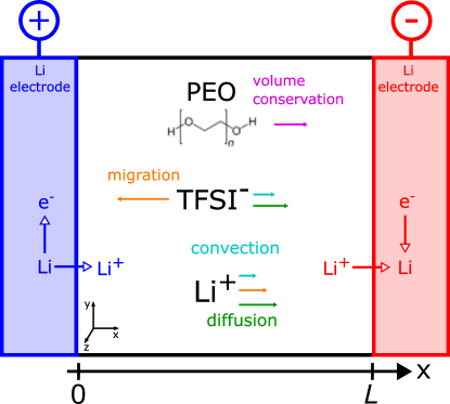
Figure 1: Illustration of the symmetric cell setup with two Li-metal electrodes and PEO/LiTFSI polymer electrolyte. The length of the cell is $L{=}$3\text{\,}\mathrm{mm}$$. The migration of anions creates concentration gradients, which in turn induce diffusion and convection fluxes.

The system polyethylene glycole (PEO) with LiTFSI salt is often used as ”benchmark” polymer for evaluation and comparison with alternate polymer electrolytes, and is among the most extensively investigated polymer electrolytes, both with respect to experimental methods and with respect to theoretical models.^{21, 63, 29, 61} Due to its widespread use, polymer electrolytes with PEO as host material are parametrized very well, which makes them attractive as reference for continuum-scale simulations.⁶¹ In addition, PEO has a relatively simple molecular structure, which facilitates atomic scale investigations.^{29, 33}.

We assume a symmetric cell set-up consisting of two Li-metal electrodes with the polymer electrolyte in between (see fig. 1 for an illustration). At the more positive electrode (left electrode in fig. 1), the surface reaction

$$\ce{Li->Li^{+}+e^{-}}$$ (42)

and at the negative electrode (right electrode in fig. 1)

$$\ce{Li^{+}+e^{-}->Li}$$ (43)

In this work, we neglect degradation processes occurring at the electrodes (e.g., SEI formation).

First, in section III.1, we state the one-dimensional equations. Second, in section III.2, we present the results obtained from a potentiostatic discharge simulation, and validate our results by a comparison with literature.⁶¹

III.1 One Dimensional Model Equations

We assume complete dissociation of the salt ions, which yields a number of three electrolyte species. Furthermore, we reduce our description to one spatial dimension on the µm-scale, where we can safely assume electroneutrality.⁴³ Thus, the set of independent material variables $\bm{\mathbb{V}}_{\ce{PEO}}$ consists only of the two variables $\bm{F}$ and $\Phi$, see eq. 36. Since $\bm{F}=\left(\begin{smallmatrix}J&0&0\\ 0&1&0\\ 0&0&1\end{smallmatrix}\right)$, the deformation gradient is completely determined by the volume ratio (see SI)

$$J=\frac{1}{c_{\ce{p}}\upnu_{\ce{p}}}=\frac{1}{1-\upnu_{\ce{LiTFSI}}c_{\ce{Li}}},$$ (44)

with $\upnu_{\ce{LiTFSI}}{=}\upnu_{\ce{Li}}{+}\upnu_{\ce{TFSI}}$. Hence, we replace $\bm{F}$ by $c_{\ce{Li}}$ as independent variable such that $\bm{\mathbb{V}}_{\ce{PEO}}{=}\{c_{\ce{Li}},\Phi\}$. The set of transport equations reads (see eqs. 38, 39, 40 and 41)

$$\partial_{t}c_{\ce{Li}}=-\mbox{div}{(\bm{N}_{\ce{Li}}^{\text{p}})}-\mbox{div}{(c_{\ce{Li}}\vec{v}^{\ce{p}})}+r_{\ce{Li}},$$ (45)

$$0=-\mbox{div}{(\bm{\mathcal{J}}^{\text{p}})}+Fr_{\ce{Li}},$$ (46)

with the polymer velocity given by (see eq. 37)

$$\mbox{div}(v_{\ce{p}})=\frac{\upnu_{\ce{TFSI}}}{F}\mbox{div}\left(\bm{\mathcal{J}}^{\ce{p}}\right)-\upnu_{\ce{LiTFSI}}\cdot\mbox{div}(N_{\ce{Li}}^{\ce{p}})+\upnu_{\ce{Li}}r_{\ce{Li}}.$$ (47)

We model the reactions at the Li electrode surfaces via source-terms based on a Butler-Volmer-Ansatz (see LABEL:subsec:SI_parameters). The fluxes appearing above are determined by eqs. 25 and 26, where the driving force $\tilde{\bm{\mathcal{F}}}_{\ce{Li}}^{\ce{p}}$ is a function of $c_{\ce{Li}}$ alone. However, by using eq. 46 in eq. 47, it follows that the flux of the Li-ions becomes $\mbox{div}\left(\bm{N}_{\ce{Li}}^{\ce{p}}\right)=r_{\ce{Li}}-\mbox{div}\left(\bm{v}^{\ce{p}}\right)/\upnu_{\ce{LiTFSI}}$. Altogether, eq. 45 thus reads

$$\partial_{t}c_{\ce{Li}}=\frac{1}{\upnu_{\ce{LiTFSI}}}\mbox{div}\left(\upnu_{\ce{p}}c_{\ce{p}}\bm{v}^{\ce{p}}\right),$$ (48)

where $c_{\ce{p}}\upnu_{\ce{p}}=1/J$, see eq. 44. Thus, the evolution of the Li-concentration is completely determined by the volume-flux of the polymer species.

Alternatively, we find

$$\partial_{t}c_{\ce{Li}}=\upnu_{\ce{p}}c_{\ce{p}}[(1-t_{\ce{Li}}^{\ce{p}})r_{\ce{Li}}-\bm{\mathcal{J}}^{\ce{p}}/F\cdot\nabla t_{\ce{Li}}^{\ce{p}}+\nabla\cdot(\mathcal{D}_{\ce{Li}}^{\ce{p}}\tilde{\bm{\mathcal{F}}}^{\ce{p}}_{\ce{Li}})]\\ -(\bm{v}^{\ce{p}}\cdot\nabla)c_{\ce{Li}}.$$ (49)

This is equivalent to the form $\partial_{t}c_{\ce{Li}}=(1-t_{\ce{Li}}^{\ce{p}})r_{\ce{Li}}\upnu_{\ce{p}}c_{\ce{p}}-(\hat{\mathbb{D}}_{\ce{Li}}\cdot\nabla)c_{\ce{Li}}$, where $\hat{\mathbb{D}}_{\ce{Li}}(\upnu_{\alpha},r_{\ce{Li}},t_{\ce{Li}}^{\ce{p}},\mathcal{D}_{\ce{Li}}^{\ce{p}})$ is an operator-valued diffusion parameter. Hence, the stationary state constitutes an equilibrium of the surface reactions with the polymer deformation and diffusive Li-transport, $(1-t_{\ce{Li}}^{\ce{p}})r_{\ce{Li}}\upnu_{\ce{p}}c_{\ce{p}}=(\hat{\mathbb{D}}_{\ce{Li}}\cdot\nabla)c_{\ce{Li}}$. Because, in general, $t_{\ce{Li}}^{\ce{p}}{\neq}$1$$ and $c_{\ce{p}}\upnu_{\ce{p}}{\neq}$0$$, the occurrence of concentration polarization is to be expected in the stationary state.

We assume constant bulk and shear moduli of the electrolyte ($K_{\ce{p}}{=}$8\text{\,}\mathrm{MPa}$$ and $G_{\ce{p}}{=}$3\text{\,}\mathrm{MPa}$$),^{64, 65, 66} and constant Flory-Huggins parameters ($\chi_{\ce{Li}\ce{TFSI}}{=}$-6$$, $\chi_{\ce{Li}\ce{p}}{=}$-20$$ and $\chi_{\ce{TFSI}\ce{p}}{=}$-15$$).⁶⁷ Only three independent transport parameters exist in this mixture. These are the ionic conductivity, one transference number and one diffusion coefficient. We parametrize them in accordance with Ref. 61. The transfer of the transport parameters from CST to our theory is described in more detail in LABEL:subsec:SI_comparison_cst, and a complete overview of our parametrization of the system is given in LABEL:subsec:SI_parameters. In LABEL:sec:SI_simulation we specify our numerical methods.

III.2 Potentiostatic Discharge Simulation

In this section we present the numerical results of our potentiostatic simulations for the as-modelled Li-cell. First, in section III.2.1, we discuss our simulation results, and, based on these observations, we give a detailed analysis of the electrolyte dynamics during discharging the cell. Second, in section III.2.2, we compare our numerical results with experimental results and with numerical results from Ref. 61.

III.2.1 Numerical Results

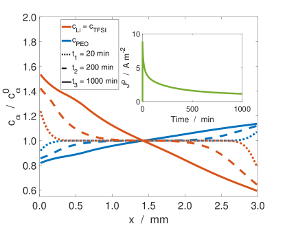
Figure 2: Species concentrations for all three electrolyte species at different time steps, normalized by their initial concentration $c_{\alpha}^{0}=c_{\alpha}(t{=}0)$. Here, the color indicates the species, and the line type indicates the time steps $t_{i}$. Note that $c_{\ce{Li}}=c_{\ce{TFSI}}$ due to our assumption of electroneutrality. The green line in the inset shows the current density (green) as function of discharge time.

In our potentiostatic discharge simulation, we apply a constant potential difference of $0.3\text{\,}\mathrm{V}$ between the positive electrode (left electrode in fig. 1) and the negative electrode (right electrode in fig. 1).

Figure 2 shows the concentration profiles of the electrolyte species, and the inset shows the profile of the discharge current $\bm{\mathcal{J}}^{\text{p}}$. In the beginning, a dynamical phase can be observed (up to $80\text{\,}\mathrm{min}$), during which the current decays exponentially from its initial peak at $\bm{\mathcal{J}}^{\text{p}}\approx$8\text{\,}\mathrm{A}\text{\,}{\mathrm{m}}^{2}$$. This dynamical phase is followed by a relaxation phase, during which the electrolyte dynamics, as indicated by $\bm{\mathcal{J}}^{p}$, slows down with time. Hence, the system is approaching a stationary state. The concentration profiles $c_{\alpha}(x,t_{i})$ of the three electrolyte species are shown at three different characteristic times $t_{i}$, and are normalized by their initial value $c_{\alpha}^{0}{=}c_{\alpha}(t{=}0)$. Note that due to the constraint of electroneutrality, the profiles of the ionic species are exactly the same for all times, i.e. $c_{\ce{Li}}{=}c_{\ce{TFSI}}$ (red curves). The first time $t_{1}{=}$20\text{\,}\mathrm{min}$$ represents the dynamical phase of enhanced electrolyte dynamics. Apparently, during this phase, concentration gradients develop near the electrodes, where the concentrations of the ions increase at the positive (left) electrode and decrease at the negative (right) electrode. Over time, this concentration polarization extends further into the electrolyte, see the profile at $t_{2}{=}$200\text{\,}\mathrm{min}$$, which corresponds to the relaxation phase of the electrolyte. Eventually, at $t_{3}{=}$1000\text{\,}\mathrm{min}$$ (end of discharge), the zones of accumulation and depletion of the ions extend throughout the complete bulk, and form almost a constant concentration gradient between the electrodes. The polymer species displays a similar, but inverse behaviour, with a concentration polarization in the opposite direction.

The corresponding species velocities are shown in fig. 3. During the complete discharge time, the anions move towards the more positive electrode at the left (yellow curves), whereas the polymer (blue curves) and the Li-ions (red curves) move towards the more negative electrode at the right. However, for all three species, the magnitudes of the species velocities are enhanced during the dynamical phase (dotted lines), and become more relaxed with increasing discharge time (dashed and solid curves).

The slight gradient of $v_{\ce{Li}}(t_{3})$ is a result of the concentration gradient for $c_{\ce{Li}}$, as shown in fig. 5.

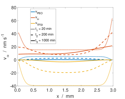
Figure 3: Species velocities at different discharge times. The different line types indicate the time step $t_{i}$, and the colors indicate the different species.

The profiles shown in figs. 2 and 3 are not perfectly linear and not symmetric (with respect to the position $x{=}$1.5\text{\,}\mathrm{mm}$$). This is because the transport parameters depend on the species concentrations, $t_{\ce{Li}}^{\ce{p}}(c_{\ce{Li}})$) and $\mathcal{D}^{\ce{p}}_{\ce{Li}}(c_{\ce{Li}})$, which influences the delicate relation between migration and diffusion.

Overall, we observe concentration polarization for all three electrolyte species. Indeed, for ionic species, such a behaviour is typical for SPEs with two mobile ions and a small transference number $t_{\ce{Li}}<1$, and is well-described in the literature.^{68, 69}

However, the role of the neutral solvent-like polymer species in such systems has not yet been intensely discussed.

Our results show that the effect of concentration polarization of the ions is accompanied by a deformation of the polymer. This deformation originates from the volume-preserving fluxes of the electrolyte species. The accumulation of TFSI- and Li-ions near the positive electrode implies a volume-flux of $c_{\ce{TFSI}}\upnu_{\ce{TFSI^{-}}}$ and $c_{\ce{Li}}\upnu_{\ce{Li}}$. This is compensated by a volume-flux $c_{\ce{p}}\upnu_{\ce{p}}$ of the polymer, towards the opposite direction, i.e. a polymer-deformation, which ensures the volumetric constraint eq. 6.

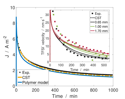
Figure 4: Comparison of our numerical results (blue line) for the current density over discharge time with experimental results (black crosses) and numerical results based on CST (yellow dashed line), both taken from Ref. 61. The inset shows the corresponding results for the species velocity $\bm{v}_{\ce{TFSI}}$ at three different locations in the electrolyte (colours). The numerical results obtained from our simulation are shown in solid lines, the crosses show the experimental results and the dashed lines show the CST results.

III.2.2 Validation

In this section, we validate our description by comparing our numerical results with experimental and numerical results presented in Ref. 61.

In fig. 4, we compare the results for the electric current density and species velocities. The blue line illustrates our numerical results for the current density, whereas the yellow dashed line and the black crosses illustrate the numerical and the experimental results from Ref. 61, respectively. The inset in fig. 4 shows the velocity profiles of the TFSI-ions at different positions during discharge.

Our results for the current density show a decay over time which is very similar to the decay exhibited by the experimental results. However, the numerical results are slightly shifted to smaller values by a constant offset during the complete discharge time. In contrast, the deviation of the CST results from experiment varies over discharge time, where, initially, both results agree very well. Overall, our description reproduces the shape of the experimental results slightly better than CST.

The inset in fig. 4 illustrates the results for the anion velocity $v_{\ce{TFSI^{-}}}(x_{i},t)$, as function of time at three different positions $x_{i}$ (indicated by colors), as obtained from our numerical simulations (solid lines), from the experiments (crosses), and from the CST-simulations (dotted lines). In the first $100\text{\,}\mathrm{min}$s, both CST and our transport model show a more rapid decrease of the $\ce{TFSI}^{-}$ velocity than the experiment. After that, CST reproduces the experimental values near the electrode very well, while our model reproduces the experimental values in the center of the electrolyte very well.

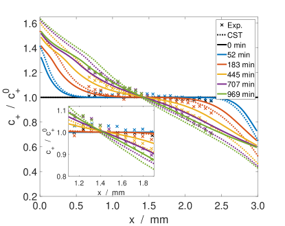
Figure 5: Comparison of our numerical results for the species concentrations (solid lines) with the experimental results (crosses) and the numerical results obtained from CST (dash line) both taken from Ref. 61. The inset focuses on the middle of the electrolyte ($x=$1.5\text{\,}\mathrm{mm}$$).

Figure 5 shows a comparison of the Li-concentration profiles at different times (distinguished by the different colors) obtained from experiment (crosses), CST (dashed lines) and from our description (solid lines). The inset highlights the central part of the electrolyte for better clarity. Up to $t=$183\text{\,}\mathrm{min}$$, CST underestimates the concentration polarization in comparison to the experimental measurements, while for larger times it overestimates it. For nearly all times, our transport model shows a slower development of the concentration polarization than the experimental results and CST. For the latest time of $969\text{\,}\mathrm{min}$ (green), the concentration profile from our transport model fits the experimental results better than CST, especially for the larger concentrations near the positive electrode.

Apparently, there exist some deviations between the numerical results obtained from our description, and from the CST description. The main difference between the two lies in the thermodynamic contribution to the species fluxes. In CST, this contribution is constituted by the concentration-dependent thermodynamic factor comprised in $\partial\upmu/\partial c\cdot\mbox{grad}\left(c\right)$, and was obtained by fitting to the experimental results.^{62, 61} This approach differs from our approach described in eq. 22. The driving forces $\partial\upmu/\partial c\cdot\mbox{grad}\left(c\right)$ appearing in our transport model are derived from fundamental physical considerations. In LABEL:sec:SI_thermodynamic_transport_contributions we present a detailed discussion of the thermodynamic transport contributions.

To summarize, our results are in good agreement with the experimental and numerical results presented in Ref. 61, which validates our theoretical description.

IV Application: Single-Ion Conducting Block Copolymer

The occurrence of concentration polarization in dual-ion conducting polymer-based electrolytes constitutes transport limitations, which hinder the battery performance (see section III.2.1).⁶⁹ Recently, it has been reported that single-ion-conducting (SIC) polymers with immobilized anions can prevent concentration polarization.⁶⁸ However, the precise impact of the immobilization of the anions on Li-transport is not yet completely clear. Here, theoretical methods can improve the understanding of these electrolytes.

In this section, we use our transport theory and investigate such a novel SIC electrolyte. We focus on a polymer-based electrolyte composed of a single-ion conducting multi-block copolymer solvated with ethylene carbonate (EC), which was recently described by Nguyen and coworkers.²³ This electrolyte exhibits promising properties, among them a good electrochemical and thermal stability, an ionic conductivity close to commercially available liquid electrolytes, and a highly reversible cycling behaviour in symmetric Lithium/Lithium-cells.

We structure our investigation into three parts. First, in section IV.1, we state the equations of motion for the SIC electrolyte. Second, in section IV.2, we show that our theory predicts that concentration polarization is negligible in SIC electrolytes. We validate this analytical finding and perform numerical discharge simulations of a symmetrical Li-metal cell (see fig. 1). Finally, in section IV.3, we present an analytical analysis of the mechanical deformation of the SIC polymer matrix.

IV.1 Model

Similar to our discussion of the PEO electrolyte in section III, we assume complete dissociation into three electrolyte species. Because the anions are chemically grafted onto the polymer backbone, we model the polymer as negative electrolyte species. The remaining two species are given by the uncharged solvent, i.e. the EC species, and by the positively charged Li-ions. We neglect microscopic details of the polymer in our continuum theory, and account for the complex structuring of the ionophobic and ionophilic blocks of the polymer chains using a volume averaged description (see eqs. 51, 52 and 50).

In contrast to the PEO based electrolyte discussed in section III, where the neutral polymer-solvent dominated the volume fraction of the electrolyte, the share of the volume fractions in the SIC is almost equally distributed among the neutral solvent (EC) and the charged polymer solvent (which is affected by migration). Hence, the polymer-based frame of reference becomes irrelevant for the SIC, and we choose the reference frame based on the volume-averaged convection velocity $\bm{v}^{\textnormal{v}}=\sum_{\alpha=1}^{\ce{N}}c_{\alpha}\upnu_{\alpha}\bm{v}_{\alpha}$ for the SIC electrolyte. As shown in Ref. 47, this has the advantage that, for the (nearly) incompressible electrolyte, the transport parameters depend hardly on the frame of reference, which facilitates the parametrization of the electrolyte and the convection is completely determined by the surface reactions,

$$\mbox{div}\left(\epsilon\bm{v}^{\text{V}}\right)=\upnu_{\ce{Li}}r_{\ce{Li}}.$$ (50)

Here, we used porous electrode theory to account for the porous ionophilic polymer-phases (which carry the Li-motion), where $\epsilon$ denotes the porosity, and $\upbeta$ denotes the Bruggemann coefficient. The volume-based transport equations for porous electrodes read,⁴⁷

$$\partial_{t}\left(\epsilon c_{\ce{Li}}\right)=-\mbox{div}{\left(\epsilon^{\upbeta}\bm{N}_{\ce{Li}}^{\text{V}}\right)}-\mbox{div}{\left(\epsilon c_{\ce{Li}}\bm{v}^{\text{V}}\right)}+r_{\ce{Li}},$$ (51)

$$0=-\mbox{div}{\left(\epsilon^{\upbeta}\bm{\mathcal{J}}^{\text{V}}\right)}+Fr_{\ce{Li}}.$$ (52)

We state the volume-based expressions for the current and flux densities in the SI, see LABEL:subsec:SI_volume_frame.

Similar to the PEO electrolyte, the three independent (volume-based) transport parameters are the electric conductvity $\kappa^{\ce{V}}$, the transference number of the Li-ions $t_{\ce{Li}}^{\ce{V}}$, and one Li-diffusion coefficient $\mathcal{D}_{\ce{Li}}^{\ce{V}}$. For more details on the volume-frame, see LABEL:subsec:SI_volume_frame or Ref. 47.

We set the elastic modulus of the SIC polymer to $E_{\ce{p}}=$249\text{\,}\mathrm{MPa}$$, which corresponds to $K_{\ce{p}}=$277\text{\,}\mathrm{MPa}$$ and $G_{\ce{p}}=$92\text{\,}\mathrm{MPa}$$.⁷⁰ For the Flory-Huggins interaction parameters we choose $\chi_{\ce{LiEC}}{=}$-5$$, $\chi_{\ce{Lip}}{=}$-20$$ and $\chi_{\ce{ECp}}{=}$-10$$. The values for the diffusion coefficient, $\mathcal{D}_{\ce{Li}}^{\ce{V}}{=}$1.94\text{\times}{10}^{-10}\text{\,}{\mathrm{m}}^{2}\text{\,}{\mathrm{s}}^{-1}$$, for the conductivity $\kappa^{\ce{V}}{=}$8.5\text{\times}{10}^{-2}\text{\,}\mathrm{S}\text{\,}{\mathrm{m}}^{-1}$$, and for the transference number, $t_{\ce{Li}}^{\ce{V}}{=}1$, are taken from Nguyen et al. (all at $T{=}$90\text{\,}\mathrm{\SIUnitSymbolCelsius}$$).²³.

The symmetric simulation setup of the Li-metal electrodes is identical to the one presented in fig. 1 for the PEO/LiTFSI electrolyte, where the electrodes are separated by a $3\text{\,}\mathrm{mm}$ thick polymer electrolyte. We discharge the battery by applying a constant voltage difference of $0.3\text{\,}\mathrm{V}$ for the whole simulation run of $1000\text{\,}\mathrm{min}$.

IV.2 Potentiostatic Discharge Simulation

In this section, we discuss the dynamics of the electrolyte during discharging the cell. First, we show that our theoretical description predicts that concentration polarization is negligible in SIC-based systems. This prediction is confirmed by experimental results.⁶⁸ Second, we validate this finding by numerical simulations.

First, we modify eq. 51, such that

$$\partial_{t}\left(\epsilon c_{\ce{Li}}\right){=}\left(1{-}t_{\ce{Li}}^{\text{V}}{-}c_{\ce{Li}}\upnu_{\ce{Li}}\right)r_{\ce{Li}}{+}\nabla\cdot(\epsilon^{\beta}\mathcal{D}_{\ce{Li}}^{\text{v}}\tilde{\bm{\mathcal{F}}}_{\ce{Li}}^{\text{v}}){-}(\epsilon\bm{v}^{\text{v}}{\cdot}\nabla)c_{\ce{Li}}.$$ (53)

Because of the immobilization of the anions, the transference number of the Li-ions is equal to one, $t_{\ce{Li}}^{\text{V}}{=}$1$$.²³ Note that the second term in brackets is a function of the Li-concentration, $\epsilon^{\beta}\mathcal{D}_{\ce{Li}}^{\text{v}}\tilde{\bm{\mathcal{F}}}_{\ce{Li}}^{\text{v}}{=}f(c_{\ce{Li}},\nabla c_{\ce{Li}})$. We make use of both properties, such that eq. 53 becomes

$$\partial_{t}(\epsilon c_{\ce{Li}})=-c_{\ce{Li}}\upnu_{\ce{Li}}r_{\ce{Li}}+(\hat{\mathbb{D}}_{\ce{Li}}\cdot\nabla)c_{\ce{Li}}.$$ (54)

Usually, the volume fraction of the Li-ions is very small $c_{\ce{Li}}\upnu_{\ce{Li}}{\ll}$1$$ . Hence, in the stationary state, there arise no relevant concentration gradients,

$$c_{\ce{Li}}\upnu_{\ce{Li}}r_{\ce{Li}}=(\hat{\mathbb{D}}_{\ce{Li}}\cdot\nabla)c_{\ce{Li}},\quad\textnormal{where}\quad c_{\ce{Li}}\upnu_{\ce{Li}}{\ll}$1$.$$ (55)

This rationalizes recent experimental observations that concentration polarization is a negligible effect in SICs.^{68, 23} We emphasize that our analytical result depends crucially on the assumption that $t_{\ce{Li}}^{\text{v}}{=}1$, and on the volume-based description.

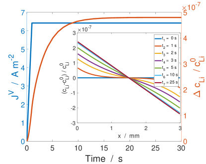
Figure 6: The current density (blue line, left axis) and the concentration difference $\Delta c_{\ce{Li}}$ (orange line, right axis) over the whole width of the electrolyte for the first $30\text{\,}\mathrm{s}$ of the simulation run. The inset shows the concentration profiles over the whole width of the electrolyte at different times (colors).

Next, we perform numerical discharge simulations of the as-described cell set-up (see fig. 1 for an illustration).

Figure 6 illustrates the temporal evolution of the electric current $\bm{\mathcal{J}}^{\text{v}}$ (blue line, left y-axis) and of the concentration differential of the Li-ions between the two electrodes $\Delta c_{\ce{Li}}(t)=|c_{\ce{Li}}(t,x{=}L)-c_{\ce{Li}}(t,x{=}$0$)|$ (red line, right y-axis), normalized by the initial concentration $c_{\ce{Li}}^{0}$. The electric current increases rapidly during the ramp up of the potential difference between the two electrodes (during the first second). However, after this initial phase, it reaches a constant plateau at $\bm{\mathcal{J}}^{\text{v}}{\approx}$6.5\text{\,}\mathrm{A}\text{\,}{\mathrm{m}}^{-2}$$ and remains constant. This corresponds to the system reaching a stationary state almost instantly. The red line (right y-axis) illustrates the behaviour of the normalized concentration differential $\Delta c_{\ce{Li}}(t)/c_{\ce{Li}}^{0}$, which serves as indicator for the occurrence of concentration polarization ($\Delta c_{\ce{Li}}(t)/c_{\ce{Li}}^{0}{\ll}$1$$ for negligible concentration polarization). The inset resolves the corresponding concentration profiles of the Li-ions over the cell length at different representative time steps $t_{i}$ during discharge. During the complete discharge time, the difference between the Li-concentration at the two electrodes is of order $\mathcal{O}(\Delta c_{\ce{Li}}/c_{\ce{Li}}^{0}){=}$1\text{\times}{10}^{-7}$$, i.e. is negligible. This behaviour is confirmed by the spatial profiles of the Li-concentrations shown in the inset. A clear gradient evolves from the left side to the right side over discharge time. In contrast to the PEO/LiTFSI electrolyte investigated in section III, the transport parameters do not depend on $c_{\ce{Li}}$. This leads to symmetric concentration gradients. Note that the spatial variation of the concentration profiles lies within the accuracy of our numerical simulation.

Altogether, we thus conclude from our numerical results that the occurrence of concentration polarization is negligible for the as-described system. This confirms our analytical prediction and is in agreement with experimental results.^{23, 68}

IV.3 Polymer Deformation

In this section, we supplement our analytical discussion from section IV.2, and focus on the deformation of the SIC polymer (see, also, LABEL:sec:SI_polymer_deformation for more details).

Polymer deformation influences the electrolyte performance. Because the concentration of the Li-ions is the only independent species concentration, it determines the polymer deformation. Therefore, polymer deformation and polarization concentration are directly coupled.

Equations 55, 54 and 53 show the influence of the Li-transference number, the volume fraction of the Li-ions, and the reaction kinetics on the occurrence of concentration polarization. We use this description and focus on the influence of these system parameters on the polymer-deformation as described by the deformation tensor $\bm{F}=\left(\begin{smallmatrix}J&0&0\\ 0&1&0\\ 0&0&1\end{smallmatrix}\right)$. Apparently, it suffices to focus on the volume ratio $J$, instead of the deformation $\bm{F}$. In the SI (see LABEL:sec:SI_polymer_deformation), we show that the volume ratio in the stationary state can be written as,

$$\mbox{grad}\left(J\right)=-\Omega\cdot j_{\ce{elde}}.$$ (56)

where $\Omega$ depends on transport-/ and material-parameters and on the driving forces, and where $j_{\ce{elde}}$ is the current due to the interface reactions.

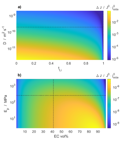
Figure 7: Polymer deformation as functions of transport parameters of the Li-ions a) and of material parameters b). The dotted lines denote the respective values used in the potentiostatic simulation in section IV.2. The colors indicate the polymer deformation as measured by the difference $\Delta J$ of volume ratios across the SIC/EC electrolyte, normalized by the initial volume ratio $J^{0}$ and the non-dimensional current density $j_{\ce{elde}}^{0}$.

Figure 7 shows the influence of transport parameters and material parameters on the deformation of the polymer as predicted by eq. 56. Here, we use the normalized variation of $J$ from the left electrode to the right electrode, i.e. $\Delta J=(J(x{=}L)-J(x{=}0)/J^{0}$, in units of the non-dimensional current density $j_{\ce{elde}}^{0}$ as measure for the polymer deformation. The non-dimensionalized current density is the current density applied to the electrodes divided by the exchange current density $j_{\ce{elde}}^{0}{=}j_{\ce{elde}}/j_{0}$, as given in the SI, LABEL:subsec:SI_parameters. The dotted lines denote the respective values used in the potentiostatic simulation in section IV.2. Figure 7 a) illustrates the influence of the transference number $t_{\ce{Li}}^{\text{V}}$ and of the diffusion coefficient $\mathcal{D}_{\ce{Li}}^{\text{V}}$ of the Li-ions on the polymer deformation. The transference number $t_{\ce{Li}}^{\text{V}}$ ranges from $0$ to $1$ and the lithium diffusion coefficient $\mathcal{D}_{\ce{Li}}^{\text{V}}$ from $0.01\cdot D^{0}$ to $10\cdot D^{0}$, where $D^{0}{=}$1.94\text{\times}{10}^{-10}\text{\,}{\mathrm{m}}^{2}\text{\,}{\mathrm{s}}^{-1}$$ is the diffusion coefficient measured by Nguyen et al.²³ Apparently, the polymer deformation decreases with increasing diffusion coefficient and with increasing lithium transference number $t_{\ce{Li}}$. Independently from the diffusion coefficient, the polymer deformation drops several orders of magnitudes to values smaller than $10^{-5}$ for $t_{\ce{Li}}^{\text{V}}{\to}1$. This reproduces our finding of negligible concentration polarization for SICs. In contrast, for $t_{\ce{Li}}^{\text{V}}{\to}0$, the flux of Li-ions in the stationary state is mainly driven by diffusion. In particular, in this regime for $t_{\ce{Li}}^{\text{V}}$, the deformation decreases with increasing diffusion coefficient. Hence, for higher values of $\mathcal{D}_{\ce{Li}}^{\text{V}}$, diffusion is fast enough to quickly equilibrate concentration gradients, yielding spatially homogeneous concentration profiles (small deformations). This is in agreement with the property that the deformation increases with decreasing diffusion coefficients.

Figure 7 b) illustrates the influence of the ethylene carbonate volume ratio and of the elastic modulus of the polymer on the deformation. Here, EC vol% ranges from $0\%$ to $99\%$, and the elastic modulus of the polymer $E_{\ce{p}}$ spans over a range of $0.01\cdot E_{\ce{p}}^{0}$ to $10\cdot E_{\ce{p}}^{0}$, with $E_{\ce{p}}^{0}=$249\text{\,}\mathrm{MPa}$$. Apparently, the polymer deformation is not very sensitive to variations of the elastic modulus for small EC volume ratios $<30\%$. However, for larger EC volume ratios $>30\%$, the influence of the elastic modulus on the resulting polymer deformation increases noticably. For the EC volume ratio however, the polymer deformation decreases at both ends of the range with a maximum in between, which results in an inverted U-shape. Since the volume ratio of the Li-ions can be neglected ($c_{\ce{Li}}\upnu_{\ce{Li}}{\ll}1$), small (large) EC volume ratios imply large (small) polymer volume ratios. Hence, a more equal distribution of the volume fraction between the EC and the polymer favors polymer deformation. This exact distribution for the largest polymer deformation also depends on the elastic modulus of the polymer.

Furthermore, it can be seen that the relative polymer deformations become much larger (up to nearly $10^{-1}$) under variations of the transport parameters (see fig. 7a), as compared with variations of the material parameters (relative polymer deformation ranges up to $10^{-5}$, see fig. 7b). This suggests that the polymer deformation depends much stronger on the transport parameters than on the material parameters. For more details, see see LABEL:sec:SI_polymer_deformation.

Finally, we compare the polymer deformation of the PEO system with the SIC results. In section III.2 it was shown that $\Delta J/\left(J^{0}\cdot j_{\ce{elde}}^{0}\right){\approx}1.8$ for the PEO/LiTFSI electrolyte. In comparison, for the SIC/EC electrolyte we found (with the parameters as denoted by the dotted lines in fig. 7) $\Delta J/\left(J^{0}\cdot j_{\ce{elde}}^{0}\right){\approx}4.2\cdot 10^{-7}$. This huge difference between the two polymer electrolytes can be explained by different transport and material parameters. The PEO/LiTFSI electrolyte exhibits a much smaller diffusion coefficient ($D^{\ce{PEO}}_{\ce{Li}}{\approx}$10\text{\times}{10}^{-11}\text{\,}{\mathrm{m}}^{2}\text{\,}{\mathrm{s}}^{-1}$$), a smaller cation transference number ($t^{\ce{PEO}}_{\ce{Li}}{\approx}0.2$) and a smaller elastic modulus ($E^{\ce{PEO}}_{\ce{p}}{=}$8\text{\,}\mathrm{MPa}$$) as compared to the SIC/EC electrolyte (where $D_{\ce{Li}}^{\ce{SIC}}{\approx}$1.94\text{\times}{10}^{-10}\text{\,}{\mathrm{m}}^{2}\text{\,}{\mathrm{s}}^{-1}$$, $t^{\ce{SIC}}_{\ce{Li}}{\approx}1$ and $E_{\ce{p}}^{\ce{SIC}}{=}$249\text{\,}\mathrm{MPa}$$). In the SI, we supplement this discussion by a more detailed analysis (see LABEL:sec:SI_polymer_deformation).

Altogether, we conclude that as consequence of the immobilization of the anions (yielding a high Li-transference number), a high diffusion coefficient and a high elastic modulus, the deformation of the SIC electrolyte is much smaller than that of other polymer-based electrolytes. This mechanical behaviour is beneficial for the performance of the electrolyte.

V Discussion

In this section we discuss the derived continuum-model for polymer electrolytes and its positioning relative to previously developed transport models.

As discussed in the introduction, see section I, polymer electrolytes comprise a wide range of materials, and exhibit solid-like properties, as well as liquid-like properties. For example, while gel polymer electrolytes behave more similar to liquid electrolytes, dry solid or composite polymer electrolytes have more similarities with solid electrolytes (like the SIC polymer electrolyte discussed in section IV). The Venn diagram shown in fig. 8 illustrates the specific properties of solid electrolytes, polymer electrolytes and liquid electrolytes, and highlights their commonalities.

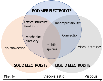
Figure 8: Venn diagram illustrating our polymer model in relation to models for viscous liquid electrolytes and solid electrolytes.

Recently, our working group has developed transport theories for highly concentrated liquid electrolytes,^{45, 51, 47} and for inorganic solid electrolytes.^{44, 52} However, these theories are limited to either viscous materials, or elastic materials, and thus constitute mutually exclusive descriptions which renders the description of viscoelastic materials, e.g. polymer electrolytes, insufficient. Our polymer theory bridges this gap and provides a description for such materials.

All three transport theories are based on the framework of rational thermodynamics (RT). Thus, they are derived from the same universal assumptions and share a common rationale. This facilitates the comparison of the three transport theories. In RT, the focal quantity is the Helmholtz free energy, which comprises material-specific properties. As consequence, the three transport theories can be differentiated via their model free energy.

From a mechanical perspective, solid electrolytes can be described as elastic materials. This implies a functional relation between the exertion of stress and the deformation (strain), which is taken into account in the model free energy. Our model describes anions as stationary lattice structure, while cations and vacancies are mobile. The immobile anions do not contribute to the mixing free energy. However, the sum of cations and vacancies has to be constant, which is a constraint not generally applicable to liquids electrolytes.

In contrast to solids, liquid electrolytes exhibit a relation between the exertion of stress and the rate of deformation (rate of strain). This accounts for viscous stresses and momentum dissipation. Our transport theory for liquid electrolytes satisfies a kinematic constraint on the volume fractions, and gives a prediction for the convection velocity in incompressible electrolytes. Convective effects due to local volume fluxes and surface reactions are important in multicomponent liquid electrolytes with high amount of salts. Here, all electrolyte species are mobilized and thus susceptible to convection and diffusion, and, if they carry charge, migration.

Finally, we put our model for polymer electrolytes into perspective. Our derived polymer electrolyte model comprises liquid-like properties. For example, our polymer description does include the motion of the polymer matrix as convection, since this is an important consideration when obtaining transport parameters from measurements. ^{71, 72, 47} Furthermore, because transport processes on the molecular scale depend on the segmental mobility of the polymer chains, ²⁹ we assume the polymer electrolyte to be incompressible. However, our polymer model does not include viscous forces, which are typical for liquid electrolytes. In addition, our model comprises also solid-like properties. For example, it allows for the description of mobile ion species and of immobilized ion-species, where the cation moves relative to a stationary and negatively charged background (as is the case for SIC/EC electrolyte in section IV). This is typical for inorganic SEs. Our polymer model also includes mechanical aspects (isotropic elasticity of the polymer matrix), which are typical for solid electrolytes.

Altogether, our polymer electrolyte model constitutes a middle ground, where deformations of the polymer play a role for transport, but are negligible for materials with a high elastic modulus (cf. section III).

VI Conclusion

In this work, we have derived a continuum transport model for polymer electrolytes using the thermodynamically consistent modelling approach already introduced for liquid and solid electrolytes as well as for ionic liquids ^{42, 43, 52, 45}. With this approach, we were able to derive a transport model that couples electro-chemical with mechanical processes while also including convection. The inclusion of thermal and viscous processes is straightforward. The formulation with respect to the polymer reference-frame made it simple to include the necessary transport parameters from other sources.

We validated our model with results from experiment and the ”standard” concentration solution theory for the ”benchmark” polymer electrolyte PEO/LiTFSI. We could show that our approach is able to reproduce the thermodynamic behaviour of the electrolyte system without the need for an empirical thermodynamic factor or activities. We also investigated a novel single-ion conducting polymer electrolyte. We showed that changes in single transport or material parameters have only negligible influence on the resulting concentration polarization for nearly single-ion conducting materials. Furthermore, we rationalized the occurrence of concentration polarization in polymer-based electrolytes, and derived an analytical description thereof.

The transport model presented in this work captures the behaviour of polymers with very different properties. It serves as a valid framework to model the behaviour of the vast range of polymer electrolytes and can fill the gap of materials treated by the already developed models for highly concentrated liquid electrolytes and ionic liquids, and inorganic solid electrolytes. Additional material processes and properties can be included by choice of a suitable free energy model.

References

- Chu and Majumdar [2012] S. Chu and A. Majumdar, Nature 488, 294 (2012).
- Bresser et al. [2018] D. Bresser, K. Hosoi, D. Howell, H. Li, H. Zeisel, K. Amine, and S. Passerini, Journal of Power Sources 382, 176 (2018).
- Armand and Taracson [2008] M. Armand and J.-M. Taracson, Nature 451, 652 (2008).
- Whittingham [2004] M. S. Whittingham, Chemical Reviews 104, 4271 (2004).
- Kim et al. [2015] J. G. Kim, B. Son, S. Mukherjee, N. Schuppert, A. Bates, O. Kwon, M. J. Choi, H. Y. Chung, and S. Park, Journal of Power Sources 282, 299 (2015).
- Weiss et al. [2021] M. Weiss, R. Ruess, J. Kasnatscheew, Y. Levartovsky, N. R. Levy, P. Minnmann, L. Stolz, T. Waldmann, M. Wohlfahrt-Mehrens, D. Aurbach, M. Winter, Y. Ein-Eli, and J. Janek, Advanced Energy Materials 11, 2101126 (2021).
- Meng et al. [2021] N. Meng, X. Zhu, and F. Lian, Particuology 60, 14 (2021).
- Janek and Zeier [2016] J. Janek and W. G. Zeier, Nature Energy 1, 16141 (2016).
- Krauskopf et al. [2020] T. Krauskopf, F. H. Richter, W. G. Zeier, and J. Janek, Chemical Reviews 120, 7745 (2020).
- Li et al. [2014] Z. Li, J. Huang, B. Yann Liaw, V. Metzler, and J. Zhang, Journal of Power Sources 254, 168 (2014).
- Cheng et al. [2015] X. B. Cheng, R. Zhang, C. Z. Zhao, F. Wei, J. G. Zhang, and Q. Zhang, Advanced Science 3, 1 (2015).
- Zheng et al. [2018] F. Zheng, M. Kotobuki, S. Song, M. O. Lai, and L. Lu, Journal of Power Sources 389, 198 (2018).
- Mindemark et al. [2018] J. Mindemark, M. J. Lacey, T. Bowden, and D. Brandell, Progress in Polymer Science 81, 114 (2018).
- Huo et al. [2019] H. Huo, Y. Chen, J. Luo, X. Yang, X. Guo, and X. Sun, Advanced Energy Materials 9, 1804004 (2019).
- Weiss et al. [2020] M. Weiss, F. J. Simon, M. R. Busche, T. Nakamura, D. Schröder, F. H. Richter, and J. Janek, Electrochemical Energy Reviews 3, 221 (2020).
- Neumann et al. [2021] A. Neumann, T. R. Hamann, T. Danner, S. Hein, K. Becker-Steinberger, E. Wachsman, and A. Latz, ACS Applied Energy Materials , 4786–4804 (2021).
- Jetybayeva et al. [2021] A. Jetybayeva, B. Uzakbaiuly, A. Mukanova, S. T. Myung, and Z. Bakenov, Journal of Materials Chemistry A 9, 15140 (2021).
- Liu et al. [2020] H. Liu, X. B. Cheng, J. Q. Huang, H. Yuan, Y. Lu, C. Yan, G. L. Zhu, R. Xu, C. Z. Zhao, L. P. Hou, C. He, S. Kaskel, and Q. Zhang, ACS Energy Letters 5, 833 (2020).
- Bocharova and Sokolov [2020] V. Bocharova and A. P. Sokolov, Macromolecules 53, 4141 (2020).
- Frenck et al. [2019] L. Frenck, G. K. Sethi, J. A. Maslyn, and N. P. Balsara, Frontiers in Energy Research 7 (2019).
- Wright [1975] P. V. Wright, British Polymer Journal 7, 319 (1975).
- Bresser et al. [2019] D. Bresser, S. Lyonnard, C. Iojoiu, L. Picard, and S. Passerini, Molecular Systems Design and Engineering 4, 779 (2019).
- Nguyen et al. [2018] H. D. Nguyen, G. T. Kim, J. Shi, E. Paillard, P. Judeinstein, S. Lyonnard, D. Bresser, and C. Iojoiu, Energy and Environmental Science 11, 3298 (2018).
- Nematdoust et al. [2020] S. Nematdoust, R. Najjar, D. Bresser, and S. Passerini, Journal of Physical Chemistry C 124, 27907 (2020).
- Butzelaar et al. [2021] A. J. Butzelaar, K. L. Liu, P. Röring, G. Brunklaus, M. Winter, and P. Theato, ACS Applied Polymer Materials 3, 1573 (2021).
- Angell et al. [1993] C. A. Angell, C. Liu, and E. Sanchez, Nature 362, 137 (1993).
- Zhou et al. [2016] W. Zhou, S. Wang, Y. Li, S. Xin, A. Manthiram, and J. B. Goodenough, Journal of the American Chemical Society 138, 9385 (2016).
- Maitra and Heuer [2007] A. Maitra and A. Heuer, Physical Review Letters 98, 1 (2007).
- Diddens et al. [2010] D. Diddens, A. Heuer, and O. Borodin, Macromolecules 43, 2028 (2010).
- Mackanic et al. [2018] D. G. Mackanic, W. Michaels, M. Lee, D. Feng, J. Lopez, J. Qin, Y. Cui, and Z. Bao, Advanced Energy Materials 8, 1 (2018).
- Liivat [2011] A. Liivat, Electrochimica Acta 57, 244 (2011).
- Ebadi et al. [2017] M. Ebadi, L. T. Costa, C. M. Araujo, and D. Brandell, Electrochimica Acta 234, 43 (2017).
- Thum et al. [2021] A. Thum, D. Diddens, and A. Heuer, Journal of Physical Chemistry C 125, 25392 (2021).
- Johansson [2015] P. Johansson, Electrochimica Acta 175, 42 (2015).
- Siekierski et al. [2007] M. Siekierski, W. Wieczorek, and K. Nadara, Electrochimica Acta 53, 1556 (2007).
- Katzenmeier et al. [2022] L. Katzenmeier, G. Manuel, A. Gagliardi, and A. S. Bandarenka, Journal of Physical Chemistry C 26, 10900–10909 (2022).
- Natsiavas et al. [2016] P. P. Natsiavas, K. Weinberg, D. Rosato, and M. Ortiz, Journal of the Mechanics and Physics of Solids 95, 92 (2016).
- Bucci et al. [2016] G. Bucci, Y. M. Chiang, and W. C. Carter, Acta Materialia 104, 33 (2016).
- Grazioli et al. [2019] D. Grazioli, O. Verners, V. Zadin, D. Brandell, and A. Simone, Electrochimica Acta 296, 1122 (2019).
- Dickinson and Smith [2020] E. J. Dickinson and G. Smith, Membranes 10, 1 (2020).
- Narayan and Anand [2021] S. Narayan and L. Anand, Journal of the Mechanics and Physics of Solids 159, 104734 (2021).
- Latz and Zausch [2011] A. Latz and J. Zausch, Journal of Power Sources 196, 3296 (2011).
- Latz and Zausch [2015] A. Latz and J. Zausch, Beilstein Journal of Nanotechnology 6, 987 (2015).
- Braun et al. [2015] S. Braun, C. Yada, and A. Latz, Journal of Physical Chemistry C 119, 22281 (2015).
- Schammer et al. [2021] M. Schammer, B. Horstmann, and A. Latz, Journal of the Electrochemical Society 168, 026511 (2021).
- von Kolzenberg et al. [2021] L. von Kolzenberg, A. Latz, and B. Horstmann, Batteries and Supercaps 202100216, 1 (2021).
- Kilchert et al. [2022] F. Kilchert, M. Lorenz, M. Schammer, P. Nürnberg, M. Schönhoff, A. Latz, and B. Horstmann, arXiv (2022), arXiv:2209.05769 .
- Lorenz et al. [2022] M. Lorenz, F. Kilchert, P. Nürnberg, M. Schammer, A. Latz, B. Horstmann, and M. Schönhoff, The Journal of Physical Chemistry Letters 13, 8761 (2022).
- Rudin [1998] A. Rudin, Elements of Polymer Science & Engineering (Elsevier, 1998).
- Ligia and Deodato [2009] G. Ligia and R. Deodato, Physicochemical Behavior and Supramolecular Organization of Polymers (Springer Netherlands, 2009).
- Schammer et al. [2022] M. Schammer, A. Latz, and B. Horstmann, The Journal of Physical Chemistry B 126, 2761 (2022).
- Becker-Steinberger et al. [2021] K. Becker-Steinberger, S. Schardt, B. Horstmann, and A. Latz, arXiv (2021), arXiv:2101.10294v1 .
- Müller [2001] I. Müller, Grundzüge der Thermodynamik (Springer Berling, Heidelberg, 2001).
- Holzapfel [2000] G. A. Holzapfel, Nonlinear Solid Mechanics (John Wiley & Sons Ltd., 2000).
- Kovetz [2000] A. Kovetz, Electromagnetic Theory (Oxford University Press Inc., New York, 2000).
- Medina and Stephany [2014] R. Medina and J. Stephany, arXiv , 1 (2014), arXiv:1404.5250 .
- de Groot and Mazur [1984] S. R. de Groot and P. Mazur, Non-Equilibrium Thermodynamics (Dover Publications, Inc., New York, 1984).
- Henjes [1993] K. Henjes, Annals of Physics 223, 277 (1993).
- Flory [1953] P. J. Flory, Principles of Polymer Chemistry (Cornell University Press, Ithaca, New York, 1953).
- Ogden and Hill [1972] R. W. Ogden and R. Hill, Proceedings of the Royal Society of London. A. Mathematical and Physical Sciences 328, 567 (1972).
- Steinrück et al. [2020] H. G. Steinrück, C. J. Takacs, H. K. Kim, D. G. MacKanic, B. Holladay, C. Cao, S. Narayanan, E. M. Dufresne, Y. Chushkin, B. Ruta, F. Zontone, J. Will, O. Borodin, S. K. Sinha, V. Srinivasan, and M. F. Toney, Energy and Environmental Science 13, 4312 (2020).
- Pesko et al. [2018] D. M. Pesko, Z. Feng, S. Sawhney, J. Newman, V. Srinivasan, and N. P. Balsara, Journal of The Electrochemical Society 165, A3186 (2018).
- Wen et al. [2003] Z. Wen, T. Itoh, T. Uno, M. Kubo, and O. Yamamoto, Solid State Ionics 160, 141 (2003).
- Jee et al. [2013] A. Y. Jee, H. Lee, Y. Lee, and M. Lee, Chemical Physics 422, 246 (2013).
- Ushakova et al. [2020] E. E. Ushakova, A. V. Sergeev, A. Morzhukhin, F. S. Napolskiy, O. Kristavchuk, A. V. Chertovich, L. V. Yashina, and D. M. Itkis, RSC Advances 10, 16118 (2020).
- Lee et al. [2022] J. Lee, M. Rottmayer, and H. Huang, Journal of Composites Science 6, 1 (2022).
- Nikolić et al. [2013] D. Nikolić, K. A. Moffat, V. M. Farrugia, A. E. Kobryn, S. Gusarov, J. H. Wosnick, and A. Kovalenko, Physical Chemistry Chemical Physics 15, 6128 (2013).
- Stolz et al. [2022] L. Stolz, S. Hochstädt, S. Röser, M. R. Hansen, M. Winter, and J. Kasnatscheew, ACS Applied Materials and Interfaces 14, 11559 (2022).
- Stolz et al. [2021] L. Stolz, G. Homann, M. Winter, and J. Kasnatscheew, Materials Today 44, 9 (2021).
- Sahu et al. [2009] A. K. Sahu, S. Pitchumani, P. Sridhar, and A. K. Shukla, Bulletin of Materials Science 32, 285 (2009).
- Rosenwinkel and Schönhoff [2019] M. P. Rosenwinkel and M. Schönhoff, Journal of The Electrochemical Society 166, A1977 (2019).
- Shao et al. [2022] Y. Shao, H. Gudla, D. Brandell, and C. Zhang, Journal of the American Chemical Society 144, 7583 (2022).