Recent Advances in Optimal Transport for Machine Learning

Abstract

Recently, Optimal Transport has been proposed as a probabilistic framework in Machine Learning for comparing and manipulating probability distributions. This is rooted in its rich history and theory, and has offered new solutions to different problems in machine learning, such as generative modeling and transfer learning. In this survey we explore contributions of Optimal Transport for Machine Learning over the period 2012 – 2022, focusing on four sub-fields of Machine Learning: supervised, unsupervised, transfer and reinforcement learning. We further highlight the recent development in computational Optimal Transport, and its interplay with Machine Learning practice.

1 Introduction

Optimal transportation theory is a well-established field of mathematics founded by the works of Gaspard Monge [1] and economist Leonid Kantorovich [2]. Since its genesis, this theory has made significant contributions to mathematics [3], physics [4], and computer science [5]. Here, we study how Optimal Transport (OT) contributes to different problems within Machine Learning (ML). Optimal Transport for Machine Learning (OTML) is a growing research subject in the ML community. Indeed, OT is useful for ML through at least two viewpoints: (i) as a loss function, and (ii) for manipulating probability distributions.

First, OT defines a metric between distributions, known by different names, such as Wasserstein distance, Dudley metric, Kantorovich metric, or Earth Mover Distance (EMD). This metric belongs to the family of Integral Probability Metrics (IPMs) (see section 2.1.1). In many problems (e.g., generative modeling), the Wasserstein distance is preferable over other notions of dissimilarity between distributions, such as the Kullback-Leibler (KL) divergence, due its topological and statistical properties.

Second, OT presents itself as a toolkit or framework for ML practitioners to manipulate probability distributions. For instance, researchers can use OT for aggregating or interpolating between probability distributions, through Wasserstein barycenters and geodesics. Hence, OT is a principled way to study the space of probability distributions.

This survey provides an updated view of how OTML in the recent years. Even though previous surveys exist [6, 7, 8, 9, 10, 11], the rapid growth of the field justifies a closer look at OTML. The rest of this paper is organized as follows. Section 2 discusses the fundamentals of different areas of ML, as well as an overview of OT. Section 3 reviews recent developments in computational optimal transport. The further sections explore OT for 4 ML problems: supervised (section 4), unsupervised (section 5), transfer (section 6), and reinforcement learning (section 7). Section 8 concludes this paper with general remarks and future research directions.

1.1 Related Work

Before presenting the recent contributions of OT for ML, we briefly review previous surveys on related themes. Concerning OT as a field of mathematics, a broad literature is available. For instance, [12] and [13], present OT theory from a continuous point of view. The most complete text on the field remains [3], but it is far from an introductory text.

As we cover in this survey, the contributions of OT for ML are computational in nature. In this sense, practitioners will be focused on discrete formulations and computational aspects of how to implement OT. This is the case of surveys [9] and [10]. While [9] serves as an introduction to OT and its discrete formulation, [10] gives a more broad view on the computational methods for OT and how it is applied to data sciences in general. In terms of OT for ML, we compare our work to [7] and [11]. The first presents the theory of OT and briefly discusses applications in signal processing and ML (e.g., image denoising). The second provides a broad overview of areas OT has contributed to ML, classified by how data is structured (i.e., histograms, empirical distributions, graphs).

Due to the nature of our work, there is a relevant level of intersection between the themes treated in previous OTML surveys and ours. Whenever that is the case, we provide an updated view of the related topic. We highlight a few topics that are new. In section 3, projection robust, structured, neural and mini-batch OT are novel ways of computing OT. We further analyze in section 8.1 the statistical challenges of estimating OT from finite samples. In section 4 we discuss recent advances in OT for structured data and fairness. In section 5 we discuss Wasserstein autoencoders, and normalizing flows. Also, the presentation of OT for dictionary learning, and its applications to graph data and natural language are new. In section 6 we present an introduction to domain adaptation, and discuss generalizations of the standard domain adaptation setting (i.e., when multiple sources are available) and transferability. Finally, in section 7 we discuss distributional and Bayesian reinforcement learning, as well as policy optimization. To the best of our knowledge, Reinforcement Learning (RL) was not present in previous related reviews.

2 Background

2.1 Optimal Transport

Let $P,Q\in\mathcal{P}(\mathbb{R}^{d})$. The Monge formulation [14] relies on a mapping $T:\mathbb{R}^{d}\rightarrow\mathbb{R}^{d}$ such that $T_{\sharp}P=Q$, where $T_{\sharp}$ is the push-forward operator associated with $T$, that is, $(T_{\sharp}P)(A)=P(T^{-1}(A))$ for $A\subset\mathbb{R}^{d}$. An OT mapping $T$ must minimize the effort of transportation,

$$\mathcal{L}_{M}(T)=\underset{\mathbf{x}\sim P}{\mathbb{E}}[c(\mathbf{x},T(\mathbf{x}))],$$

where $c:\mathbb{R}^{d}\times\mathbb{R}^{d}\rightarrow\mathbb{R}_{+}$ is called ground-cost. The Monge formulation is notoriously difficult to analyze, partly due to the constraint involving $T_{\sharp}$. A simpler formulation was presented by [2] and relies on an OT plan $\gamma:\mathbb{R}^{d}\times\mathbb{R}^{d}\rightarrow[0,1]$. Such a plan must preserve mass. For sets $A,B\subset\mathbb{R}^{d}$,

$$\gamma(\mathbb{R}^{d},B)=Q(B),\text{ and},\gamma(A,\mathbb{R}^{d})=P(A).$$

The set of all $\gamma$ sufficing these requirements is denoted by $\Gamma(P,Q)$. In this case, the effort of transportation is,

$$\mathcal{L}_{K}(\gamma)=\underset{(\mathbf{x}_{1},\mathbf{x}_{2})\sim\gamma}{\mathbb{E}}[c(\mathbf{x}_{1},\mathbf{x}_{2})].$$

This is known as Monge-Kantorovich (MK) formulation. For a theoretical proof of equivalence between Monge and Kantorovich approaches see [12, Section 1.5].

The MK formulation is easier to analyze because $\Gamma(P,Q)$ and $\mathcal{L}_{K}(\gamma)$ are linear w.r.t. $\gamma$. This remark characterizes this formulation as a linear program. As such, the MK formulation admits a dual problem [12, Section 1.2] in terms of Kantorovich potentials $\varphi:\mathbb{R}^{d}\rightarrow\mathbb{R}$ and $\psi:\mathbb{R}^{d}\rightarrow\mathbb{R}$. As such, one maximizes,

$$\mathcal{L}_{K}^{*}(\varphi,\psi)=\underset{\mathbf{x}\sim P}{\mathbb{E}}[\varphi(\mathbf{x})]+\underset{\mathbf{x}\sim Q}{\mathbb{E}}[\psi(\mathbf{x})],$$ (1)

over the constraint $\Phi_{c}=\{(\varphi,\psi):\varphi(\mathbf{x}_{1})+\psi(\mathbf{x}_{2})\leq c(\mathbf{x}_{1},\mathbf{x}_{2})\}$. When $c(\mathbf{x}_{1},\mathbf{x}_{2})=\lVert\mathbf{x}_{1}-\mathbf{x}_{2}\rVert_{2}^{2}$, the celebrated Brenier theorem [15] establishes a connection between the Monge and MK formulations: $T=\nabla\varphi$. Alternatively, when $c(\mathbf{x}_{1},\mathbf{x}_{2})=\lVert\mathbf{x}_{1}-\mathbf{x}_{2}\rVert_{1}$, one has the so-called Kantorovich-Rubinstein (KR) duality, which seeks to maximize

$$\mathcal{L}_{KR}^{*}(\varphi)=\underset{\mathbf{x}\sim P}{\mathbb{E}}[\varphi(\mathbf{x})]-\underset{\mathbf{x}\sim Q}{\mathbb{E}}[\varphi(\mathbf{x})],$$ (2)

over $\varphi\in\text{Lip}_{1}$, the set of functions with unitary Lipschitz norm.

In a parallel direction, one could see the process of transportation dynamically. This line of work was proposed in [16]. Let $\rho_{t}(\mathbf{x})=\rho(t,\mathbf{x})$ be such that $\rho(0,\cdot)=P$ and $\rho(1,\cdot)=Q$ and $v(t,\mathbf{x})$ be a velocity field. Mass preservation corresponds to the continuity equation,

$$\dfrac{\partial\rho_{t}}{\partial t}+\nabla\cdot(\rho_{t}\mathbf{v})=0,$$ (3)

and the effort of transportation can be translated as the kinetic energy throughout the transportation,

$$\mathcal{L}_{B}(\rho,\mathbf{v}) =\int_{0}^{1}\int_{\mathbb{R}^{d}}\lVert\mathbf{v}(t,\mathbf{x})\rVert^{2}\rho(t,\mathbf{x})d\mathbf{x}dt.$$ (4)

In addition, [16] established the connection between dynamic and static OT through the equations,

$$\begin{split}\mathbf{v}(t,\mathbf{x})=\nabla\varphi(t,\mathbf{x}),\\ \dfrac{\partial\varphi}{\partial t}+\dfrac{1}{2}\lVert\nabla\varphi\rVert^{2}=0.\end{split}$$ (5)

This is known as Benamou-Brenier (BB) formulation. See [12, Section 5.3] for further theoretical details.

When $c$ is a metric on $\mathbb{R}^{d}$, OT defines a metric over distributions known as Wasserstein distance $W_{c}$. This distance corresponds to the minimizer/maximizer of each effort functional defined so far. For instance, in the case of the MK formulation,

$$W_{c}(P,Q)=\underset{\gamma\in\Gamma(P,Q)}{\text{arg\,inf}}\,\underset{(\mathbf{x}_{1},\mathbf{x}_{2})\sim\gamma}{\mathbb{E}}[c(\mathbf{x}_{1},\mathbf{x}_{2})].$$

This has interesting consequences. For instance, the Wasserstein distance provides a principled way of interpolating and averaging distributions, through Wasserstein geodesics and barycenters. Concerning geodesics, as shown in [3, Chapter 7], a geodesic between $P$ and $Q$ is a distribution $P_{t}$ defined in terms of the OT plan $\gamma$,

$$P_{t}=\pi_{t,\sharp}\gamma,$$ (6)

where $\pi_{t}(\mathbf{x}_{1},\mathbf{x}_{2})=(1-t)\mathbf{x}_{1}+t\mathbf{x}_{2}$. Likewise, let $\mathcal{P}=\{P_{i}\}_{i=1}^{N}$, the Wasserstein barycenter [17] of $\mathcal{P}$, weighted by $\alpha\in\Delta_{N}=\{\mathbf{a}\in\mathbb{R}^{N}_{+}:\sum_{i=1}^{N}a_{i}=1\}$ is,

$$\mathcal{B}(\alpha;\mathcal{P})=\underset{Q}{\text{arg\,inf}}\,\sum_{i=1}^{N}\alpha_{i}W_{c}(P_{i},Q).$$ (7)

Even though this constitutes a solid theory for OT, in ML one seldom knows $P$ and $Q$ a priori. In practice, one rather has access to samples $\mathbf{x}_{i}^{(P)}\sim P$ and $\mathbf{x}_{j}^{(Q)}\sim Q$. This leads to two consequences: (i) one solves OT approximately through the available samples, and (ii) one develops a computational theory of OT. Indeed both consequences are quite challenging, which kept OT from being used in ML for a long time. We discuss these in section 3.

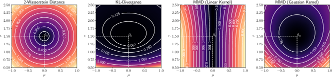
(a)

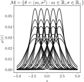
(b)

Figure 1: Comparison on how different metrics and divergences (a) calculate discrepancies on the manifold of Gaussian distributions (b).

2.1.1 Families of Probability Metrics

Probability metrics are functionals that compare probability distributions. These can be either proper metrics (e.g., the Wasserstein distance) or divergences (e.g., the KL divergence). They quantify how different the two distributions are. In probability theory, there are two prominent families of distributions metrics, Integral Probability Metrics (IPMs) [18] and $f-$divergences [19]. For a family of functions $\mathcal{F}$, an IPM [20] $d_{\mathcal{F}}$ between distributions $P$ and $Q$ is given by,

$$d_{\mathcal{F}}(P,Q)=\underset{f\in\mathcal{F}}{\text{sup}}\,\biggr{|}\underset{\mathbf{x}\sim P}{\mathbb{E}}[f(\mathbf{x})]-\underset{\mathbf{x}\sim Q}{\mathbb{E}}[f(\mathbf{x})]\biggr{|}.$$

As such, IPMs measure the distance between distributions based on the difference $P-Q$. Immediately, $\mathcal{L}_{KR}^{*}$ is an IPM for $\mathcal{F}=\text{Lip}_{1}$. Another important metric is the Maximum Mean Discrepancy (MMD) [21], defined for $\mathcal{F}=\{f\in\mathcal{H}_{k}:\lVert f\rVert_{\mathcal{H}_{k}}\leq 1\}$, where $\mathcal{H}_{k}$ is a Reproducing Kernel Hilbert Space (RKHS) with kernel $k:\mathbb{R}^{d}\times\mathbb{R}^{d}\rightarrow\mathbb{R}$. These metrics play an important role in generative modeling and domain adaptation. A third distance important in the latter field is the $\mathcal{H}-$distance [22]. Conversely, $f-$divergences measure the discrepancy between $P$ and $Q$ based on the ratio of their probabilities. For a convex, lower semi-continuous function $f:\mathbb{R}_{+}\rightarrow\mathbb{R}$ with $f(1)=0$,

$$D_{f}(P||Q)=\underset{\mathbf{x}\sim Q}{\mathbb{E}}\biggr{[}f\biggr{(}\dfrac{P(\mathbf{x})}{Q(\mathbf{x})}\biggr{)}\biggr{]},$$ (8)

where, with an abuse of notation, $P(\mathbf{x})$ (resp. $Q$) denote the density of $P$. An example of $f-$divergence is the KL divergence, with $f(u)=u\log u$.

As discussed in [20], two properties favor IPMs over f-divergences. First, $d_{\mathcal{F}}$ is defined even when $P$ and $Q$ have disjoint supports. For instance, at the beginning of training, Generative Adversarial Networks (GANs) generate poor samples, so $P_{model}$ and $P_{data}$ have disjoint support. In this sense, IPMs provide a meaningful metric, whereas $D_{f}(P_{model}||P_{data})=+\infty$ irrespective of how bad $P_{model}$ is. Second, IPMs account for the geometry of the space where the samples live. As an example, consider the manifold of Gaussian distributions $\mathcal{M}=\{\mathcal{N}(\mu,\sigma^{2}):\mu\in\mathbb{R},\sigma\in\mathbb{R}_{+}\}$. As discussed in [10, Remark 8.2], When restricted to $\mathcal{M}$, the Wasserstein distance with a Euclidean ground-cost is,

$$W_{2}(P,Q)=\sqrt{(\mu_{P}-\mu_{Q})^{2}+(\sigma_{P}-\sigma_{Q})^{2}},$$

whereas the KL divergence is associated with an hyperbolic geometry. This is shown in Figure 1. Overall, the choice of discrepancy between distributions heavily influences the success of learning algorithms (e.g., GANs). Indeed, each choice of metric/divergence induces a different geometry in the space of probability distributions, thus changing the underlying optimization problems in ML.

2.2 Machine Learning

As defined by [23], ML can be broadly understood as data-driven algorithms for making predictions. In what follows we define different problems within this field.

2.2.1 Supervised Learning

Following [24], supervised learning seeks to estimate a hypothesis $h:\mathcal{X}\rightarrow\mathcal{Y}$, $h\in\mathcal{H}$, from a feature space $\mathcal{X}$ into a label space $\mathcal{Y}$. Henceforth, we will assume $\mathcal{X}=\mathbb{R}^{d}$. $\mathcal{Y}$ is, for instance, $\{1,\cdots,n_{c}\}$, as in $n_{c}$ classes classification, or $\mathbb{R}$, in regression. The supervision in this setting comes from each $\mathbf{x}$ having an annotation $y$, coming from a ground-truth labeling function $h_{0}$. For a distribution $P$, a loss function $\mathcal{L}$, and hypothesis $h,h^{\prime}\in\mathcal{H}$, the risk functional is,

$$\mathcal{R}_{P}(h,h^{\prime})=\underset{\mathbf{x}\sim P}{\mathbb{E}}[\mathcal{L}(h(\mathbf{x}),h^{\prime}(\mathbf{x}))].$$

We further denote $\mathcal{R}_{P}(h)=\mathcal{R}_{P}(h,h_{0})$, in short. As proposed in [24], one chooses $h\in\mathcal{H}$ by risk minimization, i.e., the minimizer of $\mathcal{R}_{P}$. Nonetheless, solving a supervised learning problem with this principle is difficult, since neither $P$ nor $h_{0}$ are known beforehand. In practice, one has a dataset $\{(\mathbf{x}_{i}^{(P)},y_{i}^{(P)})\}_{i=1}^{n}$, $\mathbf{x}_{i}^{(P)}\sim P$, independently and identically distributed (i.i.d.), and $y_{i}^{(P)}=h_{0}(\mathbf{x}_{i}^{(P)})$. This is known as Empirical Risk Minimization (ERM) principle,

$$\hat{h}=\underset{h\in\mathcal{H}}{\text{arg\,min}}\,\hat{\mathcal{R}}_{P}(h)=\dfrac{1}{n}\sum_{i=1}^{n}\mathcal{L}(h(\mathbf{x}_{i}^{(P)}),y_{i}^{(P)}).$$

In addition, in deep learning one implements classifiers through Neural Networks (NNs). A deep NN, $f:\mathcal{X}\rightarrow\mathcal{Y}$ can be understood as the composition of a feature extractor $g:\mathcal{X}\rightarrow\mathcal{Z}$ and a classifier $h:\mathcal{Z}\rightarrow\mathcal{Y}$. In this sense, the gain with deep learning is that one automatizes the feature extraction process.

2.2.2 Unsupervised Learning

A key characteristic of unsupervised learning is the absence of supervision. In this sense, samples $\mathbf{x}_{i}^{(P)}\sim P$ do not have any annotation. In this survey we consider three problems in this category, namely, generative modeling, dictionary learning, and clustering.

First, generative models seek to learn to represent probability distributions over complex objects, such as images, text and time series [25]. This goal is embodied, in many cases, by learning how to reproduce samples $\mathbf{x}_{i}^{(P)}$ from an unknown distribution $P$. Examples of algorithms are GANs [25], Variational Autoencoders (VAEs) [26], and Normalizing Flows (NFs) [27].

Second, for a set of $n$ observations $\{\mathbf{x}_{i}\}_{i=1}^{n}$, dictionary learning seeks to decompose each $\mathbf{x}_{i}=\mathbf{D}^{T}\mathbf{a}_{i}$, where $\mathbf{D}\in\mathbb{R}^{k\times d}$ is a dictionary of atoms $\{\mathbf{d}_{j}\}_{j=1}^{k}$, and $\mathbf{a}_{i}\in\mathbb{R}^{k}$ is a representation. In this sense, one learns a representation for data points $\mathbf{x}_{i}$.

Finally, clustering tries to find groups of data-points in a multi-dimensional space. In this case, one assigns each $\mathbf{x}_{i}$ to one cluster $c_{i}\in\{1,\cdots,K\}$. Hence clustering is similar to classification, except that in the former, one does not know beforehand the number of classes/clusters $K$.

2.2.3 Transfer Learning

Even though the ERM framework helps to formalize supervised learning, data seldom is i.i.d. As remarked by [28], the conditions on which data were acquired for training a model are likely to change when deploying it. As a consequence, the statistical properties of the data change, a case known as distributional shift. Examples of this happen, for instance, in vision [29] and signal processing [30].

Transfer Learning (TL) was first formalized by [31], and rely on concepts of domains. A domain $\mathcal{D}=(\mathcal{X},P(X))$ is a pair of a feature space $\mathcal{X}$ and a marginal feature distribution $P(X)$. A task $\mathcal{T}=(\mathcal{Y},P(Y|X))$ is a pair of a label space $\mathcal{T}$ and a predictive distribution $P(Y|X)$. Within TL, a problem that received attention from the ML community is Unsupervised Domain Adaptation (UDA), where one has the same task, but different source and target domains $\mathcal{D}_{S}\neq\mathcal{D}_{T}$. Assuming the same feature space, this corresponds to a shift in distribution, $P_{S}(X)\neq P_{T}(X)$.

2.2.4 Reinforcement Learning

RL deals with dynamic learning scenarios and sequential decision-making. Following [32], one assumes an environment modeled through a Markov Decision Process (MDP), which is a 5-tuple $(\mathcal{S},\mathcal{A},P,R,\rho_{0},\lambda)$ of a state space $\mathcal{S}$, an action space $\mathcal{A}$, a transition distribution $P:\mathcal{S}\times\mathcal{A}\times\mathcal{S}\rightarrow\mathbb{R}$, a reward function $R:\mathcal{S}\times\mathcal{A}\rightarrow\mathbb{R}$, a distribution over the initial state $\rho_{0}$, and a discount factor $\lambda\in(0,1)$.

RL revolves around an agent acting on the state space, changing the state of the environment. The actions are chosen according to a policy $\pi:\mathcal{S}\rightarrow\mathbb{R}$, which is a distribution $\pi(\cdot|s)$ over actions $a\in\mathcal{A}$, for $s\in\mathcal{S}$. Policies can be evaluated with value functions $V_{\pi}(s_{t})$, and state-value functions $Q_{\pi}(s_{t},a_{t})$, which measure how good a state or state-action pair is under $\pi$. These are defined as,

$$\eta(\pi) =\underset{P,\pi}{\mathbb{E}}\biggr{[}\sum_{t=0}^{\infty}\lambda^{t}R(s_{t},a_{t})\biggr{]},$$ (9)

$$V_{\pi}(s) =\underset{P,\pi}{\mathbb{E}}\biggr{[}\sum_{\ell=0}^{\infty}\lambda^{\ell}R(s_{t+\ell},a_{t+\ell})|s_{t}=s\biggr{]},$$

$$Q_{\pi}(s,a) =\underset{P,\pi}{\mathbb{E}}\biggr{[}\sum_{\ell=0}^{\infty}\lambda^{\ell}R(s_{t+\ell},a_{t+\ell})|s_{t}=s,a_{t}=a\biggr{]},$$

where the expectation over $P$ and $\pi$ corresponds to $s_{0}\sim\rho_{0}$, $a_{t}\sim\pi(\cdot|s_{t})$, and $s_{t+1}\sim P(\cdot|s_{t},a_{t})$. These quantities are related through the so-called Bellman’s equation [33],

$$\mathcal{T}_{\pi}V_{\pi}(s_{t}) =\underset{P,\pi}{\mathbb{E}}[R(s_{t},a_{t})]+\gamma\underset{P,\pi}{\mathbb{E}}[V_{\pi}(s)],$$ (10)

$$\mathcal{T}_{\pi}Q_{\pi}(s_{t},a_{t}) =\underset{P,\pi}{\mathbb{E}}[R(s_{t},a_{t})]+\gamma\underset{P,\pi}{\mathbb{E}}[Q_{\pi}(s,a)],$$

where $\mathcal{T}_{\pi}$ is called Bellman operator. $Q_{\pi}$ can be learned from experience [34] (i.e., tuples $(s,a,r,s^{\prime})$). For a learning rate $\alpha_{t}>0$, the updates are as follows,

$$Q_{\pi}(s,a) \leftarrow(1-\alpha_{t})Q_{\pi}(s,a)+\alpha_{t}\biggr{(}r+\lambda V_{\pi}(s^{\prime})\biggr{)}.$$ (11)

2.3 The Curse of Dimensionality

The curse of dimensionality is a term coined by [35], and loosely refers to phenomena occurring in high-dimensions that seem counter-intuitive in low dimensions (e.g., [36]). Due to the term curse, these phenomena often have a negative connotation. For instance, consider binning $\mathbb{R}^{d}$ into $n$ distinct values [37, Section 5.11.1]. The number of distinct bins grows exponentially with the dimension. As a consequence, for assessing the probability $P(X=\mathbf{x}_{k})$ accurately, one would need exponentially many samples (i.e., imagine at least one sample per bin).

This kind of phenomenon also arises in OT. As studied by [38], for $n$ samples, the convergence rate of the empirical estimator with for the Wasserstein distance decreases exponentially with the dimension, i.e., $W_{1}(P,\hat{P})=\mathcal{O}(n^{-\nicefrac{{1}}{{d}}})$, where $f(x)=\mathcal{O}(g(x))$ if $\exists M\geq 0$ and $x_{0}$ s.t. $|f(x)|\leq Mg(x)$ $\forall x\geq x_{0}$. Henceforth we refer to the convergence rate as sample complexity. This result hinders the applicability of the Wasserstein distance for ML, but as we will discuss, other OT tools enjoy better sample complexity (see e.g., 8.1 and table I).

3 Computational Optimal Transport

Computational OT is an active field of research that has seen significant development in the past ten years. This trend is represented by publications [39, 9], and [10], and software such as [40] and [41]. These resources set the foundations for the recent spread of OT throughout ML and related fields. One has mainly three strategies in computational OT; (i) discretizing the ambient space; (ii) approximating the distributions $P$ and $Q$ from samples; (iii) assuming a parametric model for $P$ or $Q$. The first two strategies approximate distributions with a mixture of Dirac delta functions. Let $\mathbf{x}_{i}^{(P)}\sim P$ with probability $p_{i}>0$,

$$\hat{P}=\sum_{i=1}^{n}p_{i}\delta_{\mathbf{x}_{i}^{(P)}}.$$ (12)

Naturally, $\sum_{i}^{n}p_{i}=1$ or $\mathbf{p}\in\Delta_{n}$ in short. In this case, we say that $\hat{P}$ is an empirical approximation of $P$. As follows, discretizing the ambient space is equivalent to binning it, thus assuming a fixed grid of points $\mathbf{x}_{i}^{(P)}$. The sample weights $p_{i}$ correspond to the number of points that are assigned to the $i$-th bin. In this sense, the parameters of $\hat{P}$ are the weights $p_{i}$. In the literature, this strategy is known as Eulerian discretization. Conversely, one can sample $\mathbf{x}_{i}^{(P)}\overset{\text{i.i.d.}}{\sim}P$ (resp. Q). In this case, $p_{i}=\nicefrac{{1}}{{n}}$, and the parameters of $\hat{P}$ are the locations $\mathbf{x}_{i}^{(P)}$. In the literature, this strategy is known as Lagrangian discretization. Finally, one may assume $P$ follows a known law for which the Wasserstein distance has a closed formula (e.g., normal distributions).

We now discuss discrete OT. We assume $\{\mathbf{x}_{i}^{(P)}\}_{i=1}^{n}$ (resp. $\{\mathbf{x}_{j}^{(Q)}\}_{j=1}^{m}$) sampled from $P$ (resp. $Q$) with probability $p_{i}$ (resp. $q_{j}$). As in section 2.1, the Monge problem seeks a mapping $T$, that is the solution of,

$$T^{\star}=\underset{T_{\sharp}\hat{P}=\hat{Q}}{\text{arg\,min}}\,\mathcal{L}_{M}(T)=\sum_{i=1}^{n}c(\mathbf{x}_{i}^{(P)},T(\mathbf{x}_{i}^{(P)})),$$ (13)

where the constraint implies $\sum_{i\in\mathcal{I}}p_{i}=q_{j}$, for $\mathcal{I}=\{i:\mathbf{x}_{j}^{(Q)}=T(\mathbf{x}_{i}^{(P)})\}$. This formulation is non-linear w.r.t. $T$. In addition, for $m>n$, it does not have a solution. The MK formulation, on the other hand, seeks an OT plan $\gamma\in\mathbb{R}^{n\times m}$, where $\gamma_{ij}$ denotes the amount of mass transported from sample $i$ to sample $j$. In this case $\gamma$ must minimize,

$$\gamma^{\star}=\underset{\gamma\in\Gamma(\mathbf{p},\mathbf{q})}{\text{arg\,min}}\,\mathcal{L}_{K}(\gamma)=\sum_{i=1}^{n}\sum_{j=1}^{m}\gamma_{ij}c(\mathbf{x}_{i}^{(P)},\mathbf{x}_{j}^{(Q)}),$$ (14)

where $\Gamma(\mathbf{p},\mathbf{q})=\{\gamma\in\mathbb{R}^{n\times m}:\sum_{i}\gamma_{ij}=q_{j}\text{ and }\sum_{j}\gamma_{ij}=p_{i}\}$. This is a linear program, which can be solved through the Simplex algorithm [42]. Nonetheless this implies on a time complexity $\mathcal{O}(n^{3}\log n)$. Alternatively, one can use the approximation introduced by [39], by solving a regularized problem,

$$\gamma^{\star}_{\epsilon}=\underset{\gamma\in\Gamma(\mathbf{p},\mathbf{q})}{\text{arg\,min}}\,\sum_{i=1}^{n}\sum_{j=1}^{m}\gamma_{ij}c(\mathbf{x}_{i}^{(P)},\mathbf{x}_{j}^{(Q)})+\epsilon H(\gamma),$$

which provides a faster way to estimate $\gamma$. Provided either $T^{\star}$ or $\gamma^{\star}$, OT defines a metric known as Wasserstein distance, e.g., $W_{c}(\hat{P},\hat{Q})=\mathcal{L}_{K}(\gamma^{\star})$. Likewise, for $\gamma^{\star}_{\epsilon}$ one has $W_{c,\epsilon}(\hat{P},\hat{Q})=\mathcal{L}_{K}(\gamma_{\epsilon}^{\star})$. Associated with this approximation, [43] introduced the so-called Sinkhorn divergence,

$$\leavevmode\resizebox{368.57964pt}{}{$S_{c,\epsilon}(\hat{P},\hat{Q})=W_{c,\epsilon}(\hat{P},\hat{Q})-\dfrac{W_{c,\epsilon}(\hat{P},\hat{P})+W_{c,\epsilon}(\hat{Q},\hat{Q})}{2}$},$$ (15)

which has interesting properties, such as interpolating between the MMD of [21] and the Wasserstein distance. Overall, $S_{c,\epsilon}$ has 4 advantages: (i) its calculations can be done on a GPU, (ii) For $L>0$ iterations, it has complexity $\mathcal{O}(Ln^{2})$, (iii) $S_{c,\epsilon}$ is a smooth approximator of $W_{c}$ (see e.g., [44]), (iv) it has better sample complexity (see e.g., [45]).

In the following, we discuss recent innovations on computational OT. Section 3.1 present projection-based methods. Section 3.2 discusses OT formulations with prescribed structures. Section 3.3 presents OT through Input Convex Neural Networks (ICNNs). Section 3.4 explores how to compute OT between mini-batches.

3.1 Projection-based Optimal Transport

Projection-based OT relies on projecting data $\mathbf{x}\in\mathbb{R}^{d}$ into sub-spaces $\mathbb{R}^{k}$, $k<d$. A natural choice is $k=1$, for which computing OT can be done by sorting [12, chapter 2]. This is called Sliced Wasserstein (SW) distance [46, 47]. Let $\mathbb{S}^{d-1}=\{\mathbf{u}\in\mathbb{R}^{d}:\lVert\mathbf{u}\rVert_{2}^{2}=1\}$ denote the unit-sphere in $\mathbb{R}^{d}$, and $\pi_{\mathbf{u}}:\mathbb{R}^{d}\rightarrow\mathbb{R}$ denote $\pi_{\mathbf{u}}(\mathbf{x})=\langle\mathbf{u},\mathbf{x}\rangle$. The Sliced-Wasserstein distance is,

$$\text{SW}(P,Q)=\int_{\mathbb{S}^{d-1}}W_{c}(\pi_{\mathbf{u},\sharp}\hat{P},\pi_{\mathbf{u},\sharp}\hat{Q})d\mathbf{u}.$$ (16)

This distance enjoys nice computational properties. First, $W_{c}(\pi_{\mathbf{u},\sharp}P,\pi_{\mathbf{u},\sharp}Q)$ can be computed in $\mathcal{O}(n\log n)$ [10]. Second, the integration in equation 16 can be computed using Monte Carlo estimation. For samples $\{\mathbf{u}_{\ell}\}_{\ell=1}^{L}$, $\mathbf{u}_{\ell}\in\mathbb{S}^{d-1}$ uniformly,

$$\text{SW}(\hat{P},\hat{Q})=\dfrac{1}{L}\sum_{\ell=1}^{L}W_{c}(\pi_{\mathbf{u}_{\ell},\sharp}\hat{P},\pi_{\mathbf{u}_{\ell},\sharp}\hat{Q}),$$ (17)

which implies that $\text{SW}(P,Q)$ has $\mathcal{O}(Lnd+Ln\log n)$ time complexity. As shown in [48], $SW(P,Q)$ is indeed a metric. In addition, [49] and [50] proposed variants of $SW$, namely, the max-SW distance and the generalized SW distance respectively. Contrary to the averaging procedure in eq. 16, the max-SW of [49] is a mini-max procedure,

$$\text{max-SW}(P,Q)=\underset{\mathbf{u}\in\mathbb{S}^{d-1}}{\text{max}}\,W_{c}(\pi_{\mathbf{u,\sharp}}P,\pi_{\mathbf{u,\sharp}}Q).$$ (18)

This metric has the same advantage in sample complexity as the SW distance, while being easier to compute.

On another direction, [50] takes inspiration on the generalized Radon transform [51] for defining a new metric. Let $g:\mathbb{R}^{d}\times\Omega_{\theta}\rightarrow\mathbb{R}$ be a function sufficing, for $\forall\mathbf{x}\in\mathbb{R}^{d}$, $\forall\theta\in\Omega_{\theta}\text{\textbackslash}\{0\}$; (i) $g\in C^{\infty}$; (ii) $g(\mathbf{x},\lambda\theta)=\lambda g(\mathbf{x},\theta)$; (iii) $\nicefrac{{\partial g}}{{\partial\mathbf{x}}}(\mathbf{x},\theta)\neq 0$; (iv) $\text{det}(\nicefrac{{\partial^{2}g}}{{\partial x_{i}\partial\theta_{j}}})_{ij}>0$. The Generalized Sliced Wasserstein (GSW) distances are defined by,

$$\text{GSW}(P,Q)=\int_{\Omega_{\theta}}W_{c}(g_{\theta,\sharp}P,g_{\theta,\sharp}Q)d\theta.$$

One may define the max-GSW in analogy to eq. 18.

In addition, one can project samples on a sub-space $1<k<d$. For instance, [52] proposed the Subspace Robust Wasserstein (SRW) distances,

$$\text{SRW}_{k}(P,Q)=\underset{\gamma\in\Gamma(P,Q)}{\text{inf}}\,\underset{E\in\mathcal{G}_{k}}{\text{sup}}\,\underset{(\mathbf{x}_{1},\mathbf{x}_{2})\sim\gamma}{\mathbb{E}}[\lVert\pi_{E}(\mathbf{x}_{1}-\mathbf{x}_{2})\rVert^{2}_{2}],$$

where $\mathcal{G}_{k}=\{E\subset\mathbb{R}^{d}:dim(E)=k\}$ is the Grassmannian manifold of $k-$dimensional subspaces of $\mathbb{R}^{d}$, and $\pi_{E}$ denote the orthogonal projector onto $E$. This can be equivalently formulated through a projection matrix $\mathbf{U}\in\mathbb{R}^{k\times d}$, that is,

$$\text{SRW}_{k}(P,Q)=\underset{\Gamma(P,Q)}{\text{inf}}\,\underset{\begin{subarray}{c}\mathbf{U}\in\mathbb{R}^{k\times d}\\ \mathbf{U}\mathbf{U}^{T}=\mathbf{I}_{k}\end{subarray}}{\text{max}}\,\underset{(\mathbf{x}_{1},\mathbf{x}_{2})\sim\gamma}{\mathbb{E}}[\mathbf{Ux}_{1}-\mathbf{Ux}_{2}]$$

In practice, SRW_k is based on a projected super gradient method [52, Algorithm 1] that updates $\Omega=\mathbf{UU}^{T}$, for a fixed $\gamma$, until convergence. These updates are computationally complex, as they rely on eigendecomposition. Further developments using Riemannian [53] and Block Coordinate Descent (BCD) [54] circumvent this issue by optimizing over $\text{St}(d,k)=\{\mathbf{U}\in\mathbb{R}^{k\times d}:\mathbf{U}\mathbf{U}^{T}=\mathbf{I}_{k}\}$.

3.2 Structured Optimal Transport

In some cases, it is desirable for the OT plan to have additional structure, e.g., in color transfer [55] and domain adaptation [56]. Based on this problem, [57] introduced a principled way to compute structured OT through sub-modular costs.

As defined in [57], a set function $F:2^{V}\rightarrow\mathbb{R}$ is sub-modular if $\forall S\subset T\subset V$ and $\forall v\in V\text{\textbackslash}T$,

$$F(S\cup\{v\})-F(S)\geq F(T\cup\{v\})-F(T).$$

These types of functions arise in combinatorial optimization, and further OT since OT mappings and plans can be seen as a matching between 2 sets, namely, samples from $P$ and $Q$. In addition, $F$ defines a base polytope,

$$\mathcal{B}_{F}=\{G\in\mathbb{R}^{|V|}:G(V)=F(V);G(S)\leq F(S)\text{ }\forall S\subset V\}.$$

Based on these concepts, note that OT can be formulated in terms of set functions. Indeed, suppose $\mathbf{X}^{(P)}\in\mathbb{R}^{n\times d}$ and $\mathbf{X}^{(Q)}\in\mathbb{R}^{n\times d}$. In this case, $\gamma^{\star}$ or $T^{\star}$ can be interpreted as a graph with edge set $E=\{(u_{i},v_{i})\}_{i=1}^{n}$, where $u_{i}$ represents a sample in $P$ and $v_{i}$, a sample in $Q$. In this case, the cost of transportation is represented by $F(S)=\sum_{(u,v)\in S}c_{uv}$. Hence, adding a new $(u,v)$ to $S$ is the same regardless of the elements of $S$.

The insight of [57] is using the sub-modular property for acquiring structured OT plans. Through Lovász extension [58], this leads to,

$$(\gamma^{\star},\kappa^{\star})=\underset{\gamma\in\Gamma(\mathbf{p},\mathbf{q})}{\text{arg\,min}}\,\underset{\kappa\in\mathcal{B}_{F}}{\text{arg\,max}}\,\langle\gamma,\kappa\rangle_{F}.$$

A similar direction was explored by [59], who proposed to impose a low rank structure on OT plans. This was done with the purpose of tackling the curse of dimensionality in OT. They introduce the transport rank of $\gamma\in\Gamma(P,Q)$ defined as the smallest integer $K$ for which,

$$\gamma=\sum_{k=1}^{K}\lambda_{k}(P_{k}\otimes Q_{k}),$$

where $P_{k},Q_{k},k=1,\cdots,K$ are distributions over $\mathbb{R}^{d}$, and $P_{k}\otimes Q_{k}$ denotes the (independent) joint distribution with marginals $P_{k}$ and $Q_{k}$, i.e. $(P_{k}\otimes Q_{k})(\mathbf{x},\mathbf{y})=P_{k}(\mathbf{x})Q_{k}(\mathbf{y})$. For empirical $\hat{P}$ and $\hat{Q}$, $K$ coincides with the non-negative rank [60] of $\gamma\in\mathbb{R}^{n\times m}$. As follows, [59] denotes the set of $\gamma$ with transport rank at most $K$ as $\Gamma_{K}(P,Q)$ ($\Gamma_{K}(\mathbf{p},\mathbf{q})$ for empirical $\hat{P}$ and $\hat{Q}$). The robust Wasserstein distance is thus,

$$\text{FW}_{K,2}(P,Q)^{2}=\underset{\gamma\in\Gamma_{K}(P,Q)}{\text{inf}}\,\underset{(\mathbf{x}_{1},\mathbf{x})\sim\gamma}{\mathbb{E}}[\lVert\mathbf{x}_{1}-\mathbf{x}_{2}\rVert_{2}].$$

In practice, this optimization problem is difficult due to the constraint $\gamma\in\Gamma_{K}$. As follows, [59] propose estimating it using the Wasserstein barycenter $B=\mathcal{B}([\nicefrac{{1}}{{2}},\nicefrac{{1}}{{2}}];\{P,Q\})$ supported on $K$ points, that is $\{\mathbf{x}_{k}^{(B)}\}_{k=1}^{K}$, also called hubs. As follows, the authors show how to construct a transport plan in $\Gamma_{k}(P,Q)$, by exploiting the transport plans $\gamma_{1}\in\Gamma(P,B)$ and $\gamma_{2}\in\Gamma(B,Q)$. This establishes a link between the robustness of the Wasserstein distance, Wasserstein barycenters and clustering. Let $\lambda_{k}=\sum_{i=1}^{n}\gamma_{ki}^{(BP)}$ and $\mu_{k}^{(P)}=\nicefrac{{1}}{{\lambda_{k}}}\sum_{i=1}^{n}\gamma_{ki}^{(BP)}\mathbf{x}_{i}^{(P)}$, the authors in [59] propose the following proxy for the Wasserstein distance,

$$\text{FW}_{k,2}^{2}(\hat{P},\hat{Q}) =\sum_{k=1}^{K}\lambda_{k}\lVert\mu_{k}^{(P)}-\mu_{k}^{(Q)}\rVert_{2}^{2}.$$

3.3 Neural Optimal Transport

In [61], the authors proposed to leverage the so-called convexification trick of [62] for solving OT through neural nets, using the ICNN architecture proposed in [63]. Formally, an ICNN implements a function $f:\mathbb{R}^{d}\rightarrow\mathbb{R}$ such that $\mathbf{x}\mapsto f(\mathbf{x};\theta)$ is convex. This is achieved through a special structure, shown in figure 2. An $L-$layer ICNN is defined through the operations,

$$\mathbf{z}_{\ell+1}=\sigma_{\ell}(\mathbf{W}_{\ell}\mathbf{z}_{\ell}+\mathbf{A}_{\ell}\mathbf{x}+\mathbf{b}_{\ell});f(\mathbf{x};\theta)=\mathbf{z}_{L},$$

where (i) all entries of $\mathbf{W}_{\ell}$ are non-negative; (ii) $\sigma_{0}$ is convex; (iii) $\sigma_{\ell},\ell=1,\cdots,L-1$ is convex and non-decreasing. This is shown in figure 2.

Figure 2: Network architecture of an ICNN, as proposed by [63].

As follows, [61] uses [62, Theorem 2.9], for rewriting the Wasserstein distance as,

$$W_{2}(P,Q)^{2}=\mathcal{E}_{P,Q}-\underset{f\in\text{CVX}(P)}{\text{inf}}\,J(f,f^{*}),$$

where $\mathcal{E}_{P,Q}=\mathbb{E}_{\mathbf{x}\sim P}[\nicefrac{{\lVert\mathbf{x}\rVert_{2}^{2}}}{{2}}]+\mathbb{E}_{\mathbf{x}\sim Q}[\nicefrac{{\lVert\mathbf{x}\rVert_{2}^{2}}}{{2}}]$ does not depend on the $f$, and $J(f,f^{*})=\mathbb{E}_{\mathbf{x}\sim P}[f(\mathbf{x})]+\mathbb{E}_{\mathbf{x}\sim Q}[f^{*}(\mathbf{x})]$ is minimized over the set $\text{CVX}(P)=\{f:f\text{ is convex and }\mathbb{E}_{\mathbf{x}\sim P}[f(\mathbf{x})]<\infty\}$. $f^{*}$ denotes the convex conjugate of $f$, i.e., $f^{*}(\mathbf{x}_{2})=\text{sup}_{\mathbf{x}_{1}}\langle\mathbf{x}_{1},\mathbf{x}_{2}\rangle-f(\mathbf{x}_{1})$. Optimizing $J(f,f^{*})$ is, nonetheless, complicated due to the convex conjugation. The insight of [61] is to introduce a second ICNN, $g\in\text{CVX}$, that maximizes $J(f,g)$. As consequence,

$$W_{2}(P,Q)^{2} =\underset{f\in\text{CVX}(P)}{\text{sup}}\,\underset{g\in\text{CVX}(Q)}{\text{inf}}\,\mathcal{V}_{P,Q}(f,g)+\mathcal{E}_{P,Q},$$ (19)

$$\mathcal{V}_{P,Q}(f,g) =-\underset{\mathbf{x}\sim P}{\mathbb{E}}[f(\mathbf{x})]-\underset{\mathbf{x}\sim Q}{\mathbb{E}}[\langle\mathbf{x},\nabla g(\mathbf{x})\rangle-f(\nabla g(\mathbf{x}))].$$

Therefore, [61] proposes solving the sup-inf problem in eq. 19 by parametrizing $f\in\text{CVX}(P)$ and $g\in\text{CVX}(Q)$ through ICNNs. This becomes a mini-max problem, and the expectations can be approximated empirically using data from $P$ and $Q$. An interesting feature from this work is that one solves OT for mappings $f$ and $g$, rather than an OT plan. This has interesting applications for generative modeling (e.g. [64]) and domain adaptation.

3.4 Mini-batch Optimal Transport

A major challenge in OT is its time complexity. This motivated different authors [65, 43, 66] to compute the Wasserstein distance between mini-batches rather than complete datasets. For a dataset with $n$ samples, this strategy leads to a dramatic speed-up, since for $K$ mini-batches of size $m\ll n$, one reduces the time complexity of OT from $\mathcal{O}(n^{3}\log n)$ to $\mathcal{O}(Km^{3}\log m)$ [66]. This choice is key when using OT as a loss in learning [67] and inference [68]. Henceforth we describe the mini-batch framework of [69], for using OT as a loss.

Let $\mathcal{L}_{OT}$ denote an OT loss (e.g. $W_{c}$ or $S_{c,\epsilon}$). Assuming continuous distributions $P$ and $Q$, the Mini-batch OT (MBOT) loss is given by,

$$\mathcal{L}_{\text{MBOT}}(P,Q) =\underset{(\mathbf{X}^{(P)},\mathbf{X}^{(Q)})\sim P^{\otimes m}\otimes Q^{\otimes m}}{\mathbb{E}}[\mathcal{L}_{OT}(\mathbf{X}^{(P)},\mathbf{X}^{(Q)})],$$

where $\mathbf{X}^{(P)}\sim P^{\otimes m}$ indicates $\mathbf{x}_{i}^{(P)}\sim P$, $i=1,\cdots,m$. This loss inherits some properties from OT, i.e., it is positive and symmetric, but $\mathcal{L}_{\text{MBOT}}(P,P)>0$. In practice, let $\{\mathbf{x}_{i}^{(P)}\}_{i=1}^{n_{P}}$ and $\{\mathbf{x}_{j}^{(Q)}\}_{i=1}^{n_{Q}}$ be iid samples from $P$ and $Q$ respectively. Let $\mathcal{I}_{m}\subset\{1,\cdots,n_{P}\}^{m}$ denote a set of $m$ indices. We denote by $\hat{P}_{\mathcal{I}_{m}}$ to the empirical approximation of $P$ with iid samples $\mathbf{X}^{(P)}=\{\mathbf{x}_{i}^{(P)}:i\in\mathcal{I}_{m}\}$. Therefore,

$$\mathcal{L}_{\text{MBOT}}^{(k,m)}(\hat{P},\hat{Q})=\dfrac{1}{k}\sum_{(\mathcal{I}_{b},\mathcal{I}_{b}^{\prime})\in\mathbb{I}_{k}}\mathcal{L}_{OT}(\hat{P}_{\mathcal{I}_{b}},\hat{Q}_{\mathcal{I}_{b}^{\prime}}),$$ (20)

where $\mathbb{I}_{k}$ is a random set of $k$ mini-batches of size $m$ from $P$ and $Q$. This constitutes an estimator for $\mathcal{L}_{MBOT}(P,Q)$, which converges as $n$ and $k\rightarrow\infty$. We highlight 3 advantages that favor the MBOT for ML: (i) it is faster to compute and computationally scalable; (ii) the deviation bound between $\mathcal{L}_{\text{MBOT}}(P,Q)$ and $\mathcal{L}_{\text{MBOT}}^{(k,m)}$ does not depend on the dimensionality of the space; (iii) it has unbiased gradients, i.e., the expected gradient of the sample loss equals the gradient of the true loss [70].

Nonetheless, as remarked in [71], using mini-batches introduces artifacts in the OT plans, as they become less sparse. Indeed, at the level of a mini-batch, OT forces a matching between samples that would not happen at a global level. The solution proposed by [71] is to use unbalanced OT [72], as it allows for the creation and destruction of mass during transportation. This effectively makes OT more robust to outliers in mini-batches.

4 Supervised Learning

In the following, we discuss OT for supervised learning (see section 2.2.1 for the basic definitions). We divide our discussion into: (i) OT as a metric between samples; (ii) OT as a loss function; (iii) OT as a metric or loss for fairness.

In this section, we review the applications of OT for supervised learning (see section 2.2.1 for the basic definitions of this setting). We divide applications into two categories, (i) the use of OT as a metric and (ii) the use of OT as a loss, which correspond to the two following sections.

4.1 Optimal Transport as a metric

In the following, we consider OT-based distances between samples, rather than distributions of samples. This is the case when data points are modeled using histograms over a fixed grid. As such, OT can be used to define a matrix $M_{ij}$ of distances between samples $i$ and $j$, which can later be integrated in distance-based classifiers such as k-neighbors or Support Vector Machines (SVMs).

A natural example of histogram data are images. Indeed, a gray-scale image $I\in\mathbb{R}^{h\times w}$ represents a histogram over the pixel grid $(i,j)$, $i=1,\cdots,h$ and $j=1,\cdots,w$. In this sense an OT plan between two images $I_{1}$ and $I_{2}$ is a matrix $\gamma\in\mathbb{R}^{hw\times hw}$, where $\gamma_{k_{1},k_{2}}$ corresponds to how much mass is sent from pixel $k_{1}=(i,j)$ to $k_{2}=(\ell,k)$. An example of this is shown in figure 3. Such problem appears in several foundational works of OT in signal processing, such as [5] and [39].

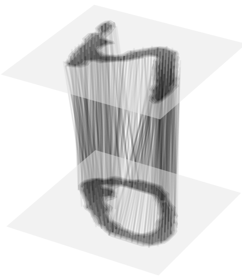
Figure 3: Transportation plan between the image $I_{1}$ of a $0$, and the image $I_{2}$ of a $5$. An edge is drawn between each pair of pixels $(i,j)$ in $I_{1}$ and $(\ell,k)$ in $I_{2}$ for which $\gamma_{k_{1}k_{2}}>0.0$.

A similar example occurs with text data. Let $\mathcal{C}=[D_{1},\cdots,D_{N}]$ represent a corpus of $N$ documents. Associated with $\mathcal{C}$ there is a vocabulary of words $\mathcal{V}=[w_{1},\cdots,w_{n}]$.. In addition, each word $w_{i}$ can be embedded in a Euclidean space through word embeddings [73]. Hence a document can be represented as,

$$\hat{P}_{\ell}=\sum_{i=1}^{n}p_{i,\ell}\delta_{\mathbf{x}_{i}^{(P_{\ell})}},$$ (21)

where $p_{i,\ell}$ is the probability of word $w_{i}$ occurring on document $P_{\ell}$ (e.g., normalized frequency), and $\mathbf{x}_{i}^{(P_{\ell})}$ is the embedding of word $w_{i}$. This corresponds to the setting for the Word Mover Distance (WMD) of [74], which relies on the Wasserstein distance between $\hat{P}_{\ell_{1}}$ and $\hat{P}_{\ell_{2}}$.

In addition, OT has been used for comparing data with a graph structure. Formally, a graph $G$ is a pair $(V,E)$ of a set of vertices and edges. Additional to the graph structure, one can have two mappings, $\ell_{f}:V\rightarrow\mathbb{R}^{n_{f}}$ and $\ell_{x}:V\rightarrow\mathbb{R}^{d}$. For each vertex $v_{i}$, $\mathbf{f}_{i}=\ell_{f}(v_{i})$ is its associated feature vector in some metric space and $\mathbf{x}_{i}=\ell_{x}(v_{i})$ its associated representation with respect to the graph structure. For a graph with $N$ vertices, one can furthermore consider a vector of vertex importance, $\mathbf{p}\in\Delta_{N}$. This constitutes the definition of a structured object [75], $\mathcal{S}=(V,E,\mathbf{F},\mathbf{X},\mathbf{p})$, $\mathbf{F}\in\mathbb{R}^{N\times n_{f}}$ and $\mathbf{X}\in\mathbb{R}^{N\times d}$. This defines multiple empirical distributions,

$$\hat{P}=\sum_{i=1}^{N}p_{i}\delta_{(\mathbf{x}_{i},\mathbf{f}_{i})}, \hat{P}^{F}=\sum_{i=1}^{N}p_{i}\delta_{\mathbf{f}_{i}}, \hat{P}^{X}=\sum_{i=1}^{N}p_{i}\delta_{\mathbf{x}_{i}}.$$

For two structured objects $\mathcal{S}_{\ell}=(V_{\ell},E_{\ell},\mathbf{F}_{\ell},\mathbf{X}_{\ell},\mathbf{h}_{\ell})$, $\ell=1,2$, a major challenge when comparing two graphs is that there is no canonical way of corresponding their vertices. In what follows we discuss three approaches.

First, one may compare 2 structured objects by their feature distributions, $\hat{P}_{1}^{F}$ and $\hat{P}_{2}^{F}$. Using this approach, one loses the information encoded by representations $\mathbf{x}_{i}$, vertices $v_{i}$ and edges $e_{uv}$. Second, one may resort to the Gromov-Wasserstein distance [76]. For a similarity function $s$, let $S_{ij}^{(\ell)}=s(\mathbf{x}_{i}^{(P_{\ell})},\mathbf{x}_{j}^{(P_{\ell})})$. An example is the shortest path distance matrix of $G_{\ell}=(V_{\ell},E_{\ell})$. The Gromov-Wasserstein (GW) distance is defined as,

$$\text{GW}(\hat{P}_{1}^{X},\hat{P}_{2}^{X})=\underset{\gamma\in\Gamma(\mathbf{p}_{1},\mathbf{p}_{2})}{\text{min}}\,\sum_{ijkl}\mathcal{L}(S_{ij}^{(1)},S_{kl}^{(2)})\gamma_{ik}\gamma_{jl},$$ (22)

where $\mathcal{L}$ is a loss function (i.e. the squared error). In comparison to the first case, one now disregards the features rather than the graph structure. Third, [75] proposed the Fused Gromov-Wasserstein (FGW) distance, which interpolates between the previous choices,

$$\text{FGW}_{\alpha}(\hat{P}_{1},\hat{P}_{2})=\underset{\gamma\in\Gamma(\mathbf{p}_{1},\mathbf{p}_{2})}{\text{min}}\,\sum_{ijkl}L_{ijkl}\gamma_{ik}\gamma_{jl},$$ (23)

$$\text{for}\,\,L_{ijkl}=(1-\alpha)c(\mathbf{f}^{(P_{1})}_{i},\mathbf{f}^{(P_{2})}_{j})+\alpha\mathcal{L}(S_{ij}^{(P_{1})},S_{kl}^{(P_{2})}),$$

4.2 Optimal Transport as a loss

In section 2.2.1 we reviewed the ERM principle, which, for a suitable loss function $\mathcal{L}$, seeks to minimize the empirical risk $\mathcal{R}_{P}(h)$ for $h\in\mathcal{H}$. In the context of neural nets, $h=h_{\theta}$ is parametrized by the weights $\theta$ of the network. An usual choice in ML is $\mathcal{L}(\hat{y}_{i},y_{i})=\sum_{k=1}^{n_{c}}y_{ik}\log\hat{y}_{ik}$ where $y_{ik}=1$ if and only if the sample $i$ belongs to class $c$, and $\hat{y}_{ik}\in[0,1]$ is the predicted probability of sample $i$ belonging to $c$. This choice of loss is related to Maximum Likelihood Estimation (MLE), and hence to the KL divergence (see [77, Chapter 4]) between $P(Y|X)$ and $P_{\theta}(Y|X)$.

As remarked by [78], this choice disregards similarities in the label space. As such, a prediction of semantically close classes (e.g. a Siberian husky and a Eskimo dog) yields the same loss as semantically distant ones (e.g. a dog and a cat). To remedy this issue, [78] proposes using the Wasserstein distance between the network’s predictions and the ground-truth vector, $\mathcal{L}(\hat{y},y)=\text{min}_{\gamma\in U(\hat{y},y)}\langle\gamma,\mathbf{C}\rangle_{F}$, where $\mathbf{C}\in\mathbb{R}^{n_{c}\times n_{c}}$ is a metric between labels.

This idea has been employed in multiple applications. For instance, [78] employs this cost between classes $k_{1}$ and $k_{2}$ as $C_{k_{1},k_{2}}=\lVert\mathbf{x}_{k_{1}}-\mathbf{x}_{k_{2}}\rVert_{2}^{2}$, where $\mathbf{x}_{k}\in\mathbb{R}^{d}$ is the $d-$dimensional embedding corresponding to the class $k$. In addition [79, 80] propose using this idea for semantic segmentation, by employing a pre-defined ground-cost reflecting the importance of each class and the severity of miss-prediction (e.g. confusing the road with a car and vice-versa in autonomous driving).

4.3 Fairness

The analysis of biases in ML algorithms has received increasing attention, due to the now widespread use of these systems for automatizing decision-making processes. In this context, fairness [81] is a sub-field of ML concerned with achieving fair treatment to individuals in a population. Throughout this section, we focus on fairness in binary classification.

The most basic notion of fairness is concerned with a sensitive or protected attribute $s\in\{0,1\}$, which can be generalized to multiple categorical attributes. We focus on the basic case in the following discussion. The values $s=0$ and $s=1$ correspond to the unfavored and favored groups, respectively. This is complementary to the theory of classification, namely, ERM (see section 2.2.1), where one wants to find $h\in\mathcal{H}$ that predicts a label $\hat{y}=h(\mathbf{x})$ to match $y\in\{0,1\}$. In this context different notions of fairness exist (e.g. [82, Table 1]). As shown in [83], these can be unified in the following equation,

$$\underset{(\mathbf{x},s,y)\sim Q}{\mathbb{E}}\biggr{[}\mathds{1}_{h(\mathbf{x})=1}\phi\biggr{(}U,\underset{(\mathbf{x},s,y)\sim Q}{\mathbb{E}}[U]\biggr{)}\biggr{]}=0,$$

where $Q=Q(X,S,Y)$. In particular, the notion of statistical parity [84] is expressed in probabilistic terms as,

$$P(h(X)=1|S=0)=P(h(X)=1|S=1).$$

As proposed by [85], this notion can be integrated into ERM through OT. Indeed, for a transformation $T$ sufficing $P(T(X)|S=1)=P(T(X)|S=0)$, a classifier trained on $T(X)$ naturally suffices the statistical parity criterion. [85] thus propose the strategy of random repair, which relies on the Wasserstein barycenter for ensuring $P(T(X)|S=1)=P(T(X)|S=0)$. Let $\mathbf{X}^{(P_{s})}=\{\mathbf{x}^{(P_{s})}_{i}:s_{i}=s\}$ where $P_{s}=P(X|S=s)$. The OT plan between $P_{0}$ and $P_{1}$ corresponds to $\gamma\in\mathbb{R}^{n_{0}\times n_{1}}$, which is itself an empirical distribution,

$$\gamma=\sum_{i=1}^{n_{0}}\sum_{j=1}^{n_{1}}\gamma_{ij}\delta_{(\mathbf{x}_{i}^{(P_{0})},\mathbf{x}_{j}^{(P_{1})})},$$

hence the geodesic or barycenter $\hat{P}_{t}$ between $\hat{P}_{0}$ and $\hat{P}_{1}$ is an empirical distribution with support,

$$\tilde{\mathbf{x}}_{t,ij}=(1-t)\mathbf{x}_{i}^{(P_{0})}+t\mathbf{x}_{j}^{(P_{1})},\forall(ij)\text{ s.t. }\gamma_{ij}>0.$$

The procedure of random repair corresponds to drawing $b_{1},\cdots,b_{n_{0}+n_{1}}\sim B(\lambda)$, where $B(\lambda)$ is a Bernoulli distribution with parameter $\lambda$. For $P_{0}$ (resp. $P_{1}$),

$$\mathbf{X}^{(P_{0})} =\bigcup_{i=1}^{n_{0}}\begin{cases}\{\mathbf{x}_{i}^{(P_{0})}\}&\text{ if }b_{i}=0\\ \{\mathbf{x}_{t,ij}:\gamma_{ij}>0\}&\text{ if }b_{i}=1\end{cases},$$

where the amount of repair $\lambda$ regulates the trade-off between fairness ($\lambda=1$) and classification performance ($\lambda=0$). In addition, $t=\nicefrac{{1}}{{2}}$, so as to avoid disparate impact.

In another direction, one may use OT for devising a regularization term to enforce fairness in ERM. Two works follow this strategy, namely [86] and [87]. In the first case, the authors explore fairness in representation learning (see for instance section 2.2.1). In this sense, let $f=h\circ g$, be the composition of a feature extractor $g$ and a classifier $h$. Therefore [86] proposes minimizing,

$$(h^{\star},g^{\star})=\underset{h,g}{\text{arg\,min}}\,\dfrac{1}{n}\sum_{i=1}^{n}\mathcal{L}(h(g(\mathbf{x}_{i})),y_{i})+\beta d(P_{0},P_{1}),$$

for $\beta>0$, $P_{0}=P(X|S=0)$ (resp $S=1$) and $d$ being either the MMD or the Sinkhorn divergence (see sections 2.1). On another direction, [87] considers the output distribution $P_{s}=P(h(g(X))|S=s)$. Their approach is more general, as they suppose that attributes can take more than 2 values, namely $s\in\{1,\cdots,N_{S}\}$. Their insight is that the output distribution should be transported to the distribution closest to each group’s conditional, namely $P_{k}=P(h(g(X))|S=k)$. This corresponds to $P_{\bar{s}}=\mathcal{B}(\alpha;{P_{k}}_{k=1}^{n_{s}})$, $\alpha_{s}=\nicefrac{{n_{s}}}{{n}}$. As in [86], the authors enforce this condition through regularization, namely,

$$\underset{h,g}{\text{min}}\,\dfrac{1}{n}\sum_{i=1}^{n}\mathcal{L}(h(g(\mathbf{x}_{i})),y)+\beta\sum_{k=1}^{N_{S}}\dfrac{n_{k}}{n}W_{2}(P_{k},\bar{P}).$$

Finally, we remark that OT can be used for devising a statistical test of fairness [83]. To that end, consider,

$$\mathcal{F}=\biggr{\{}Q:\underset{(\mathbf{x},s,y)\sim Q}{\mathbb{E}}\biggr{[}\mathds{1}_{h(\mathbf{x})=1}\phi\biggr{(}U,\underset{(\mathbf{x},s,y)\sim Q}{\mathbb{E}}[U]\biggr{)}\biggr{]}=0\biggr{\}},$$

the set of distributions $Q$ for which a classifier $h$ is fair. Now, let $\{(\mathbf{x}_{i},s_{i},y_{i})\}_{i=1}^{N}$ be samples from a distribution $P$. Let $\hat{P}=\nicefrac{{1}}{{n}}\sum_{i=1}^{n}\delta_{(\mathbf{x}_{i},s_{i},y_{i})}$. The fairness test of [83] consists on a hypothesis test with $\mathcal{H}_{0}:P\in\mathcal{F}$ and $\mathcal{H}_{1}:P\notin\mathcal{F}$. The test is then based on,

$$d(P,\mathcal{F})=\underset{Q\in\mathcal{F}}{\text{inf}}\,W_{2}(P,Q),$$

for which on rejects $\mathcal{H}_{0}$ if $t=n\times d(P,\mathcal{F})>\eta_{1-\alpha}$, where $\eta_{1-\alpha}$ is the $(1-\alpha)\times 100\%$ quantile of the generalized chi-squared distribution.

5 Unsupervised Learning

In this section, we discuss unsupervised learning techniques that leverage the Wasserstein distance as a loss function. We consider three cases: generative modeling (section 5.1), representation learning (section 5.2) and clustering (section 5.3).

5.1 Generative Modeling

There are mainly three types of generative models that benefit from OT, namely, GANs (section 5.1.1), VAEs (section 5.1.2) and normalizing flows (section 5.1.3). As discussed in [88, 89], OT provides an unifying framework for these principles through the Minimum Kantorovich Estimator (MKE) framework, introduced by [90], which, given samples from $P_{0}$, tries to find $\theta$ that minimizes $W_{2}(P_{\theta},P_{0})$.

5.1.1 Generative Adversarial Networks

(a)

(b)

(c)

Figure 4: Architecture of different generative models studiend in this section; (a) GANs; (b) VAEs; (c) AAEs.

GAN is a NN architecture proposed by [25] for sampling from a complex probability distribution $P_{0}$. The principle behind this architecture is building a function $g_{\theta}$, that generates samples in a input space $\mathcal{X}$ from latent vectors $\mathbf{z}\in\mathcal{Z}$, sampled from a simple distribution $Q$ (e.g. $\mathcal{N}(0,\sigma^{2})$). A GAN is composed by two networks: a generator $g_{\theta}:\mathcal{Z}\rightarrow\mathcal{X}$, and a discriminator $h_{\xi}:\mathcal{X}\rightarrow[0,1]$. $\mathcal{X}$ is called the input space (e.g. image space) and $\mathcal{Z}$ is the latent space (e.g. an Euclidean space $\mathbb{R}^{p}$). The architecture is shown in Figure 4 (a). Following [25], the GAN objective function is,

$$\mathcal{L}_{G}(\theta,\xi)=\underset{\mathbf{x}\sim P_{0}}{\mathbb{E}}[\log(h_{\xi}(\mathbf{x}))]+\underset{\mathbf{z}\sim Q}{\mathbb{E}}[\log(1-h_{\xi}(g_{\theta}(\mathbf{z})))],$$

which is a minimized w.r.t. $\theta$ and maximized w.r.t. $\xi$. In other words, $h_{\xi}$ is trained to maximize the probability of assigning the correct label to $\mathbf{x}$ (labeled 1) and $g_{\theta}(\mathbf{z})$ (labeled 0). $g_{\theta}$, on the other hand, is trained to minimize $\log(1-h_{\xi}(g_{\theta}(\mathbf{z})))$. As consequence it minimizes the probability that $h_{\xi}$ guesses its samples correctly.

As shown in [25], for an optimal discriminator $h_{\xi^{\star}}$, the generator cost is equivalent to the so-called Jensen-Shannon (JS) divergence. In this sense, [91] proposed the Wasserstein GAN (WGAN) algorithm, which substitutes the JS divergence by the KR metric (equation 2),

$$\underset{\theta}{\text{min}}\,\underset{h_{\xi}\in\text{Lip}_{1}}{\text{max}}\,\mathcal{L}_{W}(\theta,\xi)=\underset{\mathbf{x}\sim P_{0}}{\mathbb{E}}\biggr{[}h_{\xi}(\mathbf{x})\biggr{]}-\underset{\mathbf{z}\sim Q}{\mathbb{E}}\biggr{[}h_{\xi}(g_{\theta}(\mathbf{z}))\biggr{]}.$$

Nonetheless, the WGAN involves maximizing $\mathcal{L}_{W}$ over $h_{\xi}\in\text{Lip}_{1}$. Nonetheless, this is not straightforward for NNs. Possible solutions are: (i) clipping the weights $\xi$ [91]; (ii) penalizing the gradients of $h_{\xi}$ [92]; (iii) normalizing the spectrum of the weight matrices [93]. Surprisingly, even though (ii) and (iii) improve over (i), several works have confirmed that the WGAN and its variants do not estimate the Wasserstein distance [94, 95, 96].

In another direction, one can calculate $\nabla_{\theta}W_{p}(P_{\theta},P_{0})$ using the primal problem (equation 14). To do so, [43] and further [69] consider estimating $W_{p}(P_{\theta},P_{0})$ through averaging the loss over mini-batches (see section 3.4). For calculating derivatives $\nabla_{\theta}W_{p}(P_{\theta},P_{0})$, one has two approaches. First, [43] advocate to back-propagate through Sinkhorn iterations. This is numerically unstable and computationally complex. Second, as discussed in [97], [98], one can use the Envelope Theorem [99] to take derivatives of $W_{p}$. In its primal form, it amounts to calculate $\gamma^{\star}=\text{OT}_{\epsilon}(\mathbf{p},\mathbf{q},\mathbf{C})$ then differentiating w.r.t. $\mathbf{C}$.

In addition, as discussed in [43], an Euclidean ground-cost is likely not meaningful for complex data (e.g., images). The authors thus propose learning a parametric ground cost $(\mathbf{C}_{\eta})_{ij}=\lVert f_{\eta}(\mathbf{x}_{i}^{(P_{\theta})})-f_{\eta}(\mathbf{x}^{(P_{0})}_{j})\rVert$, where $f_{\eta}:\mathcal{X}\rightarrow\mathcal{Z}$ is a NN that learns a representation for $\mathbf{x}\in\mathcal{X}$. Overall the optimization problem proposed by [43] is,

$$\underset{\theta}{\text{min}}\,\underset{\eta}{\text{max}}\,S_{c_{\eta},\epsilon}(P_{\theta},P_{0}).$$ (24)

We stress the fact that engineering/learning the ground-cost $c_{\eta}$ is important for having a meaningful metric between distributions, since it serves to compute distances between samples. For instance, the Euclidean distance is known to not correlate well with perceptual or semantic similarity between images [100].

Finally, as in [101, 49, 50, 102], one can employ sliced Wasserstein metrics (see section 3.1). This has two advantages: (i) computing the sliced Wasserstein distances is computationally less complex, (ii) these distances are more robust w.r.t. the curse of dimensionality [103, 104]. These properties favour their usage in generative modeling, as data is commonly high dimensional.

5.1.2 Autoencoders

In a parallel direction, one can leverage autoencoders for generative modeling. This was introduced in [26], who proposed using stochastic encoding and decoding functions. Let $f_{\eta}:\mathcal{X}\rightarrow\mathcal{Z}$ be an encoder network. Instead of mapping $\mathbf{z}=f_{\eta}(\mathbf{x})$ deterministically, $f_{\eta}$ predicts a mean $\mathbf{m}_{\eta}(\mathbf{x})$ and a variance $\sigma_{\eta}(\mathbf{x})^{2}$ from which the code $\mathbf{z}$ is sampled, that is, $\mathbf{z}\sim Q_{\eta}(\mathbf{z}|\mathbf{x})=\mathcal{N}(\mathbf{m}_{\eta}(\mathbf{x}),\sigma_{\eta}(\mathbf{x})^{2})$. The stochastic decoding function $g_{\theta}:\mathcal{Z}\rightarrow\mathcal{X}$ works similarly for reconstructing the input $\hat{\mathbf{x}}$. This is shown in figure 4 (b). In this framework, the decoder plays the role of generator.

The VAE framework is built upon variational inference, which is a method for approximating probability densities [105]. Indeed, for a parameter vector $\theta$, generating new samples $\mathbf{x}$ is done in two steps: (i) sample $\mathbf{z}$ from the prior $Q(\mathbf{z})$ (e.g. a Gaussian), then (ii) sample $\mathbf{x}$ from the conditional $P_{\theta}(\mathbf{x}|\mathbf{z})$. The issue comes from calculating the marginal,

$$P_{\theta}(\mathbf{x})=\int Q(\mathbf{z})P_{\theta}(\mathbf{x}|\mathbf{z})d\mathbf{z},$$

which is intractable. This hinders the MLE, which relies on $\log P_{\theta}(\mathbf{x})$. VAEs tackle this problem by first considering an approximation $Q_{\eta}(\mathbf{z}|\mathbf{x})\approx P_{\theta}(\mathbf{z}|\mathbf{x})$. Secondly, one uses the Evidence Lower Bound (ELBO),

$$\text{ELBO}(Q_{\eta}) =\underset{\mathbf{z}\sim Q_{\eta}}{\mathbb{E}}[\log P_{\theta}(\mathbf{x},\mathbf{z})]-\underset{\mathbf{z}\sim Q_{\eta}}{\mathbb{E}}[\log Q_{\eta}(\mathbf{z})],$$

instead of the log-likelihood. Indeed, as shown in [26], the ELBO is a lower bound for the log-likelihood. As follows, one turns to the maximization of the ELBO, which can be rewritten as,

$$\mathcal{L}(\theta,\eta)=\underset{\mathbf{x}\sim P_{0}}{\mathbb{E}}\biggr{[}\underset{\mathbf{z}\sim Q_{\eta}}{\mathbb{E}}[\log P_{\theta}(\mathbf{x}|\mathbf{z})]-\text{KL}(Q_{\eta}\lVert Q)\biggr{]}.$$ (25)

A somewhat middle ground between the frameworks of [25] and [26] is the Adversarial Autoencoder (AAE) architecture [106], shown in figure 4 (c). AAEs are different from GANs in two points, (i) an encoder $f_{\eta}$ is added, for mapping $\mathbf{x}\in\mathcal{X}$ into $\mathbf{z}\in\mathcal{Z}$; (ii) the adversarial component is done in the latent space $\mathcal{Z}$. While the first point puts the AAE framework conceptually near VAEs, the second shows similarities with GANs.

Based on both AAEs and VAEs, [107] proposed the Wasserstein Autoencoder (WAE) framework, which is a generalization of AAEs. Their insight is that, when using a deterministic decoding function $g_{\theta}$, one may simplify the MK formulation,

$$\underset{\gamma\in\Gamma}{\text{inf}}\,\underset{(\mathbf{x}_{1},\mathbf{x}_{2})\sim\gamma}{\mathbb{E}}[c(\mathbf{x}_{1},\mathbf{x}_{2})]=\underset{Q_{\eta}=Q}{\text{inf}}\,\underset{\mathbf{x}\sim P_{0}}{\mathbb{E}}\biggr{[}\underset{\mathbf{z}\sim Q_{\eta}}{\mathbb{E}}[c(\mathbf{x},g_{\theta}(\mathbf{z}))]\biggr{]}.$$

As follows, [107] suggests enforcing the constraint in the infimum through a penalty term $\Omega$, leading to,

$$\mathcal{L}(\theta,\eta)=\underset{\mathbf{x}\sim P_{0}}{\mathbb{E}}\biggr{[}\underset{\mathbf{z}\sim Q_{\eta}}{\mathbb{E}}[c(\mathbf{x},g_{\theta}(\mathbf{z}))]\biggr{]}+\lambda\Omega(Q_{\eta},Q),$$

for $\lambda>0$. This expression is minimized jointly w.r.t. $\theta$ and $\eta$. As choices for the penalty $\Omega$, [107] proposes using either the JS divergence, or the MMD distance. In the first case the formulation falls back to a mini-max problem much alike the AAE framework. A third choice was proposed by [108], which relies on the Sinkhorn loss $S_{c,\epsilon}$, thus leveraging the work of [43].

5.1.3 Continuous Normalizing Flows

OT contributes to the class of generative models known as NFs through its dynamic formulation (e.g. section 2.1 and equations 3 through 5). Especially, they contribute to a specific class of NFs known as Continuous Normalizing Flows (CNFs). We thus focus on this class of algorithms. For a broader review, we refer the readers to [27]. Normalizing flows rely on the chain rule for computing changes in probability distributions exactly. Let $\mathbf{T}:\mathbb{R}^{d}\rightarrow\mathbb{R}^{d}$ be a diffeomorphism. If, for $\mathbf{z}\sim Q$ and $\mathbf{x}\sim P$, $\mathbf{z}=\mathbf{T}(\mathbf{x})$, one has,

$$\log P(\mathbf{x}) =\log Q(\mathbf{z})-\log|\det\nabla\mathbf{T}^{-1}|.$$

Following [27], a NF is characterized by a sequence of diffeomorphisms $\{T_{i}\}_{i=1}^{N}$ that transform a simple probability distribution (e.g. a Gaussian distribution) into a complex one. If one understands this sequence continuously, they can be modeled through dynamic systems. In this context, CNFs are a class of generative models based on dynamic systems,

$$\mathbf{z}(\mathbf{x},0)=\mathbf{x}\text{, and, }\dot{\mathbf{z}}(\mathbf{x},t)=\mathbf{F}_{\theta}(\mathbf{z}(\mathbf{x},t)).$$ (26)

which is an Ordinary Differential Equation (ODE). Henceforth we denote $\mathbf{z}_{t}(\mathbf{x})=\mathbf{z}(\mathbf{x},t)$. Using Euler’s method and setting $\mathbf{z}_{0}=\mathbf{x}$, one can discretize equation 26 as $\mathbf{z}_{n+1}=\mathbf{z}_{n}+\tau\mathbf{F}_{\theta}(\mathbf{z}_{n})$, for a step-size $\tau>0$. This equation is similar to the ResNet structure [109]. Indeed, this is the insight behind the seminal work of [110], who proposed the Neural ODE (NODE) algorithm for parametrizing ODEs through NNs. CNFs are thus the intersection of NFs with NODE.

According to [110], if a Random Variable (RV) $\mathbf{z}(\mathbf{x},t)$ suffices equation 26, then its log-probability follows,

$$\dfrac{\partial}{\partial t}\log|\det\nabla\mathbf{z}| =\text{Tr}(\nabla_{\mathbf{z}}\mathbf{F}_{\theta})=\text{div}(\mathbf{F}_{\theta}).$$ (27)

With this workaround, minimizing the negative log-likelihood amounts to minimizing,

$$\sum_{i=1}^{n}-\log Q(\mathbf{z}_{T}(\mathbf{x}_{i}))-\int_{0}^{T}\text{div}(\mathbf{F}_{\theta}(\mathbf{z}_{t}(\mathbf{x}_{i})))dt,$$ (28)

which can be solved using the automatic differentiation [110]. One limitation of CNFs is that the generic flow can be highly irregular, having unnecessarily fluctuating dynamics. As remarked by [111], this can pose difficulties to numerical integration. These issues motivated the proposition of two regularization terms for simpler dynamics. The first term is based dynamic OT. Let,

$$\rho_{t}=\mathbf{z}_{t,\sharp}P=\dfrac{1}{n}\sum_{i=1}^{n}\delta_{\mathbf{z}_{t}(\mathbf{x}_{i})},$$

and recalling the concepts in section 2.1, this simplifies eq. 4,

$$\underset{\theta}{\text{min}}\, \mathcal{L}(\theta)=\dfrac{1}{n}\sum_{i=1}^{n}\int_{0}^{T}\lVert\mathbf{F}_{\theta}(\mathbf{z}_{t}(\mathbf{x}_{i}))\rVert^{2}dt,$$ (29)

subject to $$\mathbf{z}_{0}=\mathbf{x}\text{, and }\mathbf{z}_{T,\sharp}P=Q,$$

where $\lVert\mathbf{F}_{\theta}(\mathbf{z}_{t}(\mathbf{x}_{i}))\rVert^{2}$ is the kinetic energy of the particle $\mathbf{x}_{i}$ at time $t$, and $\mathcal{L}$ to the whole kinetic energy. In addition, $\rho_{t}$ has the properties of an OT map. Among these, OT enforces that: (i) the flow trajectories do not intersect, and (ii) the particles follow geodesics w.r.t. the ground cost (e.g. straight lines for an Euclidean cost), thus enforcing the regularity of the flow. Nonetheless, as [111] remarks, these properties are enforced only on training data. To effectively generalize them, the authors propose a second regularization term, that consists on the Frobenius norm of the Jacobian,

$$\Omega(\mathbf{F})=\dfrac{1}{n}\sum_{i=1}^{n}\lVert\nabla\mathbf{F}_{\theta}(\mathbf{z}_{T}(\mathbf{x}_{i}))\rVert_{F}^{2}.$$ (30)

Thus, the Regularized Neural ODE (RNODE) algorithm combines equation 27 with the penalties in equations 29 and 30. Ultimately, this is equivalent to minimizing the KL divergence KL$(\mathbf{z}_{T,\sharp}P\lVert Q)$ with the said constraints.

5.2 Dictionary Learning

Dictionary learning [112] represents data $\mathbf{X}\in\mathbb{R}^{n\times d}$ through a set of $K$ atoms $\mathbf{D}\in\mathbb{R}^{k\times d}$ and $n$ representations $\mathbf{A}\in\mathbb{R}^{n\times k}$. For a loss $\mathcal{L}$ and a regularization term $\Omega$,

$$\underset{\mathbf{D},\mathbf{A}}{\text{arg\,min}}\,\dfrac{1}{n}\sum_{i=1}^{n}\mathcal{L}(\mathbf{x}_{i},\mathbf{D}^{T}\mathbf{a}_{i})+\lambda\Omega(\mathbf{D},\mathbf{A}).$$ (31)

In this setting, the data points $\mathbf{x}_{i}$ are approximated linearly through the matrix-vector product $\mathbf{D}^{T}\mathbf{a}_{i}$. In other words, $\mathbf{X}\approx\mathbf{AD}$. The practical interest is finding a faithful and sparse representation for $\mathbf{X}$. In this sense, $\mathcal{L}$ is often the Euclidean distance, and $\Omega(\mathbf{A})$ the $\ell_{1}$ or $\ell_{0}$ norm of vectors.

When the elements of $\mathbf{X}$ are non-negative, the dictionary learning problem is known as Non-negative Matrix Factorization (NMF) [113]. This scenario is particularly useful when data $\mathbf{X}$ are histograms, that is, $\mathbf{x}_{i}\in\Delta_{d}$. As such, one needs to choose an appropriate loss function for histograms. OT provides such a loss, through the Wasserstein distance [114], in which case the problem can be solved using BCD: for fixed $\mathbf{D}$, solve for $\mathbf{A}$, and vice-versa.

Nonetheless, the BCD iterations scale poorly since NMF is equivalent to solving $n$ linear programs with $d^{2}$ variable. To bypass the complexity involved with the exact calculation of the Wasserstein distance, [114] resort to the wavelet approximation of [115], which has closed form. On another direction, [116] propose using the Sinkhorn algorithm [39] for NMF. Besides reducing complexity, using the Sinkhorn distance $W_{c,\epsilon}$ makes NMF smooth, thus gradient descent methods can be applied successfully. The optimization problem of Wasserstein Dictionary Learning (WDL) reads as,

$$\underset{\mathbf{D},\mathbf{A}}{\text{arg\,min}}\,\dfrac{1}{N}\sum_{i=1}^{N}W_{c,\epsilon}(\mathbf{x}_{i},\mathbf{D}^{T}\mathbf{a}_{i})+\lambda\Omega(\mathbf{D},\mathbf{A}),$$ (32)

subject to $\mathbf{AD}\in(\Delta_{d})^{N}$. Assuming $\mathbf{a}_{i}\in\Delta_{k}$ implies that $\mathbf{D}^{T}\mathbf{a}_{i}$ represents a weighted average of dictionary elements. This can be understood as a barycenter under the Euclidean metric. This remark motivated [117] to use the Wasserstein barycenter $\mathcal{B}(\mathbf{a}_{i},\mathbf{D})$ of histograms in $\mathbf{D}$, with weights $\mathbf{a}_{i}$, for approximating $\mathbf{x}_{i}$, that is,

$$\underset{\mathbf{D},\mathbf{A}}{\text{arg\,min}}\,\sum_{i=1}^{N}W_{c,\epsilon}(\mathcal{B}(\mathbf{a}_{i},\mathbf{D}),\mathbf{x}_{i})+\lambda\Omega(\mathbf{D},\mathbf{A})$$

Graph Dictionary Learning. An interesting use case of this framework is Graph Dictionary Learning (GDL) (see section 4.1). Let $\{G_{\ell}:(\mathbf{h}_{\ell},\mathbf{S}^{(\ell)})\}_{\ell=1}^{N}$ denote a dataset of $N$ graphs encoded by their node similarity matrices $\mathbf{S}^{(\ell)}\in\mathbb{R}^{n_{\ell}\times n_{\ell}}$, and histograms over nodes $\mathbf{h}_{\ell}\in\Delta_{n_{\ell}}$. [118] proposes,

$$\underset{\{\mathbf{S}_{k}\}_{k=1}^{K},\{\mathbf{a}_{\ell}\}_{\ell=1}^{N}}{\text{arg\,min}}\,\sum_{\ell=1}^{N}\text{GW}_{2}^{2}\biggr{(}\mathbf{S}^{(\ell)},\sum_{k=1}^{K}a_{\ell,k}\mathbf{S}^{(k)}\biggr{)}-\lambda\lVert\mathbf{a}_{\ell}\rVert_{2}^{2},$$

in analogy to eq. 31, using the GW distance (see eq. 22) as loss function. Parallel to this line of work, [119] proposes Gromov-Wasserstein Factorization (GWF), which approximates $\mathbf{S}^{(\ell)}$ non-linearly through GW-barycenters [120].

Topic Modeling. Another application of dictionary learning consists on topic modeling [121], in which a set of documents is expressed in terms of a dictionary of topics weighted by mixture coefficients. As explored in section 4.1, documents can be interpreted as probability distributions over words (e.g., eq. 21). In this context [122] proposes an OT-inspired algorithm for learning a set of distributions $\mathcal{Q}=\{\hat{Q}_{k}\}_{k=1}^{K}$ over words in the whole vocabulary. In this sense, each $\hat{Q}_{k}$ is a topic. Learning is based on a hierarchical OT problem,

$$\underset{\{\mathbf{q}_{k}\}_{k=1}^{K},\mathbf{b},\gamma}{\text{min}}\, \sum_{k=1}^{K}\sum_{i=1}^{N}\gamma_{ik}W_{2,\epsilon}(\hat{Q}_{k},\hat{P}_{i})-H(\gamma),$$

where $\hat{Q}_{k}=\sum_{v=1}^{V}q_{k,v}\delta_{\mathbf{x}_{v}^{(Q_{k})}}$, and $\mathbf{b}=[b_{1},\cdots,b_{K}]$ is the coefficient of topic $k$. In this sense $\sum_{i}\gamma_{ik}=b_{k}$, and $\sum_{k}\gamma_{ik}=p_{i}$, with $p_{i}=\nicefrac{{n_{i}}}{{V}}$ is the proportion of words in document $\hat{P}_{i}$.

5.3 Clustering

Clustering is a problem within unsupervised learning that deals with the aggregation of features into groups [123]. From the perspective of OT, this is linked to the notion of quantization [124, 125]; Indeed, from a distributional viewpoint, given $\mathbf{X}^{(P)}\in\mathbb{R}^{n\times d}$, quantization corresponds to finding the matrix $\mathbf{X}^{(Q)}\in\mathbb{R}^{K\times d}$ minimizing $W_{2}(P,Q)$. This has been explored in a number of works, such as [126, 127] and [128]. In this sense, OT serves as a framework for quantization/clustering, thus allowing for theoretical results such as convergence bounds for the $K$-means algorithm [125].

Conversely, the Wasserstein distance can be used for performing $K$-means in the space of distributions. Given $P_{1},\cdots,P_{N}$, this consists on finding $\mathbf{R}\in\{0,1\}^{N\times K}$ and $\mathcal{Q}=\{Q_{k}\}_{k=1}^{K}$ such that,

$$(\mathbf{R}^{\star},\mathcal{Q}^{\star})=\underset{\mathbf{R},\mathcal{Q}}{\text{arg\,min}}\,\sum_{i=1}^{N}\sum_{k=1}^{K}r_{ik}W_{2}(P_{i},Q_{k}).$$

This problem can be optimized in two steps: (i) one sets $r_{ik}=1$ if $Q_{k}$ is the closest distribution to $P_{i}$ (w.r.t. $W_{2}$); (ii) one computes the centroids using $\mathcal{P}_{k}=\{P_{i}:r_{ik}=1\}$. In this case $Q_{k}=\mathcal{B}(\nicefrac{{1}}{{\sum_{i}r_{ik}}};\mathcal{P}_{k})$. This formulation is related to the robust clustering of [129], who proposed a version of the Wasserstein barycenter-based clustering analogous to the trimmed $K-$means of [130].

6 Transfer Learning

As discussed in section 2.2.3, TL is a framework for ML, when data follows different probability distributions. The most general case of distributional shift corresponds to $P_{S}(X,Y)\neq P_{T}(X,Y)$. Since $P(X,Y)=P(X)P(Y|X)=P(Y)P(X|Y)$, three types of shift may occur [131]: (i) covariate shift, that is, $P_{S}(X)\neq P_{T}(X)$, (ii) concept shift, namely, $P_{S}(Y|X)\neq P_{T}(Y|X)$ or $P_{S}(X|Y)\neq P_{T}(X|Y)$, and (iii) target shift, for which $P_{S}(Y)\neq P_{T}(Y)$.

This section is structured as follows. In sections 6.1 and 6.2 we present how OT is used in both shallow and deep Domain Adaptation (DA). For a broader view on the subject, encompassing other methods than OT-based, one may consult surveys on deep domain adaptation such as [132] and [29]. In section 6.3 we present how OT has contributed to more general DA settings (e.g. multi-source and heterogeneous DA). Finally, section 6.4 covers methods for predicting the success of TL methods.

6.1 Shallow Domain Adaptation

Assuming $P_{S}(X)=P_{T}(\phi(X))$ for an unknown, possibly nonlinear mapping $\phi$, OT can be used for matching $P_{S}$ and $P_{T}$. Since the Monge problem may not have a solution for discrete distributions, [56] proposes doing so through the Kantorovich formulation, i.e., by calculating $\gamma=\text{OT}(\mathbf{p}_{S},\mathbf{p}_{T},\mathbf{C})$. The OT plan $\gamma$ has an associated mapping known as the barycentric mapping or projection [55, 56, 133],

$$T_{\gamma}(\mathbf{x}^{(P_{S})}_{i})=\underset{\mathbf{x}\in\mathbb{R}^{d}}{\text{arg\,min}}\,\sum_{j=1}^{n_{T}}\gamma_{ij}c(\mathbf{x},\mathbf{x}^{(P_{T})}_{j})$$ (33)

The case where $c(\mathbf{x}_{1},\mathbf{x}_{2})=\lVert\mathbf{x}_{1}-\mathbf{x}_{2}\rVert^{2}_{2}$ is particularly interesting, as $\mathbf{T}_{\gamma}$ has closed-form in terms of the support $\mathbf{X}^{(P_{T})}\in\mathbb{R}^{n_{T}\times d}$ of $\hat{P}_{T}$, $\hat{\mathbf{X}}_{S}=\mathbf{T}_{\gamma}(\mathbf{X}^{(P_{S})})=\text{diag}(\mathbf{p}_{S})^{-1}\gamma\mathbf{X}^{(P_{T})}$. As follows, each point $\mathbf{\mathbf{x}}_{S}^{i}$ is mapped into $\hat{\mathbf{x}}_{S}^{i}$, which is a convex combination of the points $\mathbf{x}_{T}^{j}$ that receives mass from $\mathbf{x}_{S}^{i}$, namely, $\gamma_{ij}>0$. This effectively generates a new training dataset $\{(\hat{\mathbf{x}}_{i}^{(P_{S})},y_{i}^{(P_{S})})\}_{i=1}^{n_{S}}$, which hopefully leads to a classifier $\hat{f}_{S}$ that works well on $\mathcal{D}_{T}$. An illustration is shown in Figure 5.

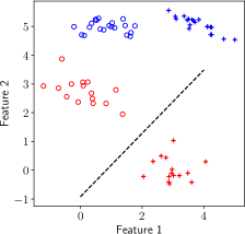
(a)

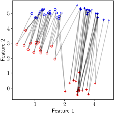
(b)

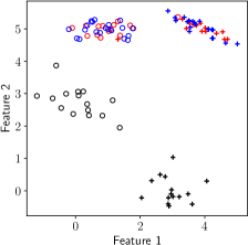
(c)

Figure 5: OTDA methodology: (a) Source (red) and target (blue) samples follow different distributions; A classifier (dashed black line) fit on source is not adequate for target; (b) OT plan visualization. An edge connects source and target points $(ij)$ whenever $\gamma_{ij}>0$. (c) $T_{\gamma}$ generates samples on target domain (red).

Nonetheless, the barycentric projection works by mapping $\mathbf{x}_{i}^{(P_{S})}$ to the convex hull of $\{\mathbf{x}_{j}^{(P_{T})}:\gamma_{ij}>0\}$. As consequence, if $\mathbf{x}_{i}^{(P_{S})}$ sends mass to $\mathbf{x}_{j}^{(P_{T})}$ from a different class, it ends up on the wrong side of the classification boundary. Based on this issue, [56] proposes using class-based regularizers for inducing class sparsity on the transportation plan, namely, $\gamma_{ij}\neq 0\iff y_{i}^{(P_{S})}=y_{j}^{(P_{T})}$. This is done by introducing additional regularizers,

$$\gamma^{\star}=\underset{\gamma\in U(\mathbf{p}_{S},\mathbf{p}_{T})}{\text{arg\,min}}\,\langle\mathbf{C},\gamma\rangle_{F}-\epsilon H(\gamma)+\eta\Omega(\gamma;\mathbf{y}^{(P_{S})},\mathbf{y}^{(P_{T})}).$$

where $\Omega$ is the class sparsity regularizer. Here we discuss 2 cases proposed in [56]: (i) semi-supervised and (ii) group-lasso. The semi-supervised regularizer assumes that $y^{(P_{T})}$ are known at training time, so that,

$$\begin{split}\Omega(\gamma;\mathbf{y}^{(P_{S})},\mathbf{y}^{(P_{T})})&=\sum_{i=1}^{n_{S}}\sum_{j=1}^{n_{T}}\gamma_{ij}\delta(y^{(P_{S})}_{i}-y^{(P_{T})}_{j}),\end{split}$$ (34)

this corresponds to adding $\eta$ to the ground-cost entries $C_{ij}$ which $y^{(P_{S})}_{i}\neq y^{(P_{T})}_{j}$. In practice [56] proposes $\eta\rightarrow\infty$, which implies that transporting samples from different classes is infinitely costly. Nonetheless, in many cases $\mathbf{y}^{(P_{T})}$ is not known during training. This leads to proxy regularizers such as the group-lasso. The idea is that samples $\mathbf{x}_{S}^{i}$ and $\mathbf{x}_{S}^{j}$ from the same class should be transported nearby. Hence, the group-lasso is defined as,

$$\Omega(\gamma;\mathbf{y}^{(P_{S})})=\sum_{j}\sum_{c=0}^{n_{c}-1}\lVert\gamma_{\mathcal{I}_{c}j}\rVert_{2},$$

where, for a given class $c$, $\mathcal{I}_{c}$ corresponds to the indices of the samples of that given class. In this notation, $\gamma_{\mathcal{I}_{c}j}$ is a vector with as much components as samples in the class $c$.

In addition, note that the barycentric projection $T_{\gamma}$ is defined only on the support of $\hat{P}_{S}$. When the number of samples $n_{S}$ or $n_{T}$ is large, finding $\gamma$ is not feasible (either due to time or memory constraints). This is the case in many applications in deep learning, as datasets are usually large. A few workarounds exist, such as interpolating the values of $T_{\gamma}$ through nearest neighbors [55], or parametrizing $T_{\gamma}$ (e.g. linear or based on a kernel) [134, 133].

So far, note that one assumes a weaker version of the covariate shift hypothesis. One may as well assume that the shift occurs on the joint distributions $P_{S}(X,Y)$, $P_{T}(X,Y)$, then try to match those. In UDA this is not directly possible, since the labels from $P_{T}(X,Y)$ are not available. A workaround was introduced in [135], where the authors propose a proxy distribution $P_{T}^{h}(X,h(X))$:

$$\hat{P}_{T}^{h}=\dfrac{1}{n_{T}}\sum_{j=1}^{n_{T}}\delta_{\mathbf{x}^{(P_{T})}_{j},h(\mathbf{x}^{(P_{T})}_{j})}.$$

where $h\in\mathcal{H}$ is a classifier. As follows, [135] propose minimizing the Wasserstein distance $W_{c}(\hat{P}_{S},\hat{P}_{T}^{h})$ over possible classifiers $h\in\mathcal{H}$. This yields a joint minimization problem,

$$\underset{\begin{subarray}{c}h\in\mathcal{H}\\ \gamma\in U(\mathbf{p}_{S},\mathbf{p}_{T})\end{subarray}}{\text{min}}\,\sum_{i=1}^{n_{S}}\sum_{j=1}^{n_{T}}c(\mathbf{x}^{(P_{S})}_{i},y^{(P_{S})}_{i},\mathbf{x}^{(P_{T})}_{j})\gamma_{ij}+\lambda\Omega(h).$$

The cost $c$ can be designed in terms of two factors, a feature loss $c_{f}(\mathbf{x}^{(P_{S})}_{i},\mathbf{x}^{(P_{T})}_{j})$ (e.g. the Euclidean distance), and a label loss $c_{\ell}(y^{(P_{S})}_{i},h(\mathbf{x}^{(P_{T})}_{j}))$ (e.g. the Hinge loss). As proposed in [135], the importance of $c_{f}$ and $c_{\ell}$ can be controlled by a parameter $\alpha$,

$$C_{ij} =\alpha c_{f}(\mathbf{x}_{i}^{(P_{S})},\mathbf{x}_{j}^{(P_{T})})+c_{\ell}(y_{i}^{(P_{S})},h(\mathbf{x}_{j}^{(P_{T})})).$$

6.2 Deep Domain Adaptation

Recalling the concepts of section 2.2.1, a deep NN is a composition $f=h_{\xi}\circ g_{\theta}$ of a feature extractor $g$ with parameters $\theta$, and a classifier $h_{\xi}$ with parameters $\xi$. The intuition behind deep DA is to force the feature extractor to learn domain invariant features. Given $\mathbf{x}_{i}^{(P_{S})}\sim P_{S}$ and $\mathbf{x}_{j}^{(P_{T})}\sim P_{T}$, an invariant feature extractor $g_{\theta}$ should suffice,

$$(g_{\theta})_{\sharp}\hat{P}_{S}=\dfrac{1}{n_{S}}\sum_{i=1}^{n_{S}}\delta_{\mathbf{z}_{i}^{(P_{S})}}\overset{W_{c}}{\approx}\dfrac{1}{n_{T}}\sum_{j=1}^{n_{T}}\delta_{\mathbf{z}_{j}^{(P_{T})}}=(g_{\theta})_{\sharp}\hat{P}_{T},$$

where $\mathbf{z}_{i}^{(P_{S})}=g_{\theta}(\mathbf{x}_{i}^{(P_{S})})$ (resp. $\hat{P}_{T}$), and $\hat{P}_{S}\overset{W_{c}}{\approx}\hat{P}_{T}$ means $W_{c}(\hat{P}_{S},\hat{P}_{T})\approx 0$. This implies that, after the application of $g_{\theta}$, distributions $\hat{P}_{S}$ and $\hat{P}_{T}$ are close. In this sense, this condition is enforced by adding an additional term to the classification loss function (e.g. the MMD as in [136]). In this context, [137] proposes the Domain Adversarial Neural Network (DANN) algorithm, based on the loss function,

$$\mathcal{L}_{\text{DANN}}(\theta,\xi,\eta) =\hat{\mathcal{R}}_{P_{S}}(h_{\xi}\circ g_{\theta})-\lambda\mathcal{L}_{\mathcal{H}}(\theta,\eta),$$

where $\mathcal{L}_{\mathcal{H}}$ denotes,

$$\dfrac{1}{n_{S}}\sum_{i=1}^{n_{S}}\log h_{\eta}(\mathbf{z}_{i}^{(P_{S})}))+\dfrac{1}{n_{T}}\sum_{j=1}^{n_{T}}\log(1-h_{\eta}(\mathbf{z}_{j}^{(P_{T})})),$$

and $h_{\eta}$ is a supplementary classifier, that discriminates between source (labeled $0$) and target (labeled $1$). The DANN algorithm is a mini-max optimization problem,

$$\underset{\theta,\xi}{\text{min}}\,\underset{\eta}{\text{max}}\,\mathcal{L}_{\text{DANN}}(\theta,\xi,\eta),$$

so as to minimize classification error and maximize domain confusion. This draws a parallel with the GAN algorithm of [25], presented in section 5.1.1. This remark motivated [138] for using the Wasserstein distance instead of $d_{\mathcal{H}}$. Their algorithm is called Wasserstein Distance Guided Representation Learning (WDGRL). The Wasserstein domain adversarial loss is then,

$$\mathcal{L}_{W}(\theta,\eta) =\dfrac{1}{n_{S}}\sum_{i=1}^{n_{S}}h_{\eta}(g_{\theta}(\mathbf{x}^{(P_{S})}_{i}))-\dfrac{1}{n_{T}}\sum_{j=1}^{n_{T}}h_{\eta}(g_{\theta}(\mathbf{x}^{(P_{T})}_{j})).$$

Following our discussion on KR duality (see section 2.1) as well as the Wassers tein GAN (see section 5.1.1), one needs to maximize $\mathcal{L}_{d}$ over $h_{\eta}\in\text{Lip}_{1}$. [138] proposes doing so using the gradient penalty term of [92],

$$\underset{\theta}{\text{min}}\,\underset{\xi}{\text{min}}\,\hat{\mathcal{R}}_{P_{S}}(h_{\xi}\circ g_{\theta})+\lambda_{2}\underset{\eta}{\text{max}}\,\mathcal{L}_{W}(\theta,\eta)-\lambda_{1}\Omega(h_{\eta}),$$

where $\lambda_{1}$ controls the gradient penalty term, and $\lambda_{2}$ controls the importance of the domain loss term.

Finally, we highlight that the Joint Distribution Optimal Transport (JDOT) framework can be extended to deep DA. First, one includes the feature extractor $g_{\theta}$ in the ground-cost,

$$C_{ij}(\theta,\xi) =\alpha\lVert\mathbf{z}_{i}^{(P_{S})}-\mathbf{z}_{j}^{(P_{T})}\rVert^{2}+c_{\ell}(y_{i}^{(P_{S})},h_{\xi}(\mathbf{z}_{j}^{(P_{T})})),$$

second, the objective function includes a classification loss $\mathcal{R}_{P_{S}}$, and the OT loss, that is,

$$\mathcal{L}_{JDOT}(\theta,\xi) =\hat{\mathcal{R}}_{P_{S}}(h_{\xi}\circ g_{\theta})+\sum_{i=1}^{n_{S}}\sum_{j=1}^{n_{T}}\gamma_{ij}C_{ij}(\theta,\xi),$$ (35)

which is jointly minimized w.r.t. $\gamma\in\mathbb{R}^{n_{S}\times n_{T}}$, $\theta$ and $\xi$. [67] proposes minimizing $\mathcal{L}_{\text{JDOT}}$ jointly w.r.t. $\theta$ and $\xi$, using mini-batches (see section 3.4). Nonetheless, the authors noted that one needed large mini-batches for a stable training. To circumvent this issue [71] proposed using unbalanced OT, allowing for smaller batch sizes and improved performance.

6.3 Generalizations of Domain Adaptation

In this section we highlight 2 generalizations of the DA problem. First, Multi-Source Domain Adaptation (MSDA) (e.g. [139]), deals with the case where source data comes from multiple, distributionally heterogeneous domains, namely $P_{S_{1}},\cdots,P_{S_{K}}$. Second, Heterogeneous Domain Adaptation (HDA), is concerned with the case where source and target domain data live in incomparable spaces (e.g. [140]).

For MSDA, [141] proposes using the Wasserstein barycenter for building an intermediate domain $\hat{P}_{B}=\mathcal{B}(\alpha;\{\hat{P}_{S_{k}}\}_{k=1}^{N_{S}})$ (see equation 7), for $\alpha_{k}=\nicefrac{{1}}{{N_{S}}}$. Since $\hat{P}_{B}\neq\hat{P}_{T}$, the authors propose using an additional adaptation step for transporting the barycenter towards the target. In a different direction, [142] proposes the Weighted JDOT algorithm, which generalizes the work of [135] for MSDA,

$$\underset{\alpha,g_{\theta},h_{\xi}}{\text{min}}\,\dfrac{1}{k}\sum_{k=1}^{K}\hat{\mathcal{R}}_{P_{S_{k}}}(h_{\xi}\circ g_{\theta})+W_{c_{\theta,\xi}}(\hat{P}_{T}^{h_{\xi}},\sum_{k=1}^{K}\alpha_{k}\hat{P}_{S_{k}}).$$

For HDA, Co-Optimal Transport (COOT) [140] tackles DA when the distributions $\hat{P}_{S}$ and $\hat{P}_{T}$ are supported on incomparable spaces, that is, $\mathbf{X}^{(P_{S})}\in\mathbb{R}^{n_{S}\times d_{S}}$ and $\mathbf{X}^{(P_{T})}\in\mathbb{R}^{n_{T}\times d_{T}}$, $n_{S}\neq n_{T}$ and $d_{S}\neq d_{T}$. The authors strategy relies on the GW OT formalism,

$$(\gamma^{(s)},\gamma^{(f)})=\underset{\begin{subarray}{c}\gamma^{(s)}\in\Gamma(\mathbf{w}_{S},\mathbf{w}_{T})\\ \gamma^{(f)}\in\Gamma(\mathbf{v}_{S},\mathbf{v}_{T})\end{subarray}}{\text{min}}\,\sum_{ijkl}L(\mathbf{X}_{i,k}^{(P_{S})},\mathbf{X}_{j,l}^{(P_{T})})\gamma_{ij}^{(s)}\gamma_{ij}^{(f)},$$

where $\gamma^{(s)}\in\mathbb{R}^{n_{S}\times n_{T}}$ and $\gamma^{(f)}\in\mathbb{R}^{d_{S}\times d_{T}}$ are OT plans between samples and features, respectively. Using $\gamma^{(s)}$, one can estimate labels on the target domain using label propagation [143]: $\hat{\mathbf{Y}}^{(P_{T})}=\text{diag}(\mathbf{p}_{T})^{-1}(\gamma^{(s)})^{T}\mathbf{Y}^{(P_{S})}$.

6.4 Transferability

Transferability concerns the task of predicting whether TL will be successful. From a theoretical perspective, different IPMs bound the target risk $\mathcal{R}_{P_{T}}$ by the source risk $\mathcal{R}_{P_{S}}$, such as the $\mathcal{H}$, Wasserstein and MMD distances (see e.g., [22, 144, 131]). Furthermore there is a practical interest in accurately measuring transferability a priori, before training or fine-tuning a network. A candidate measure coming from OT is the Wasserstein distance, but in its original formulation it only takes features into account.  [145] propose the Optimal Transport Dataset Distance (OTDD), which relies on a Wasserstein-distance based metric on the label space,

$$\text{OTDD}(P_{S},P_{T}) =\underset{\gamma\in\Gamma(P_{S},P_{T})}{\text{arg\,min}}\,\underset{(\mathbf{z}_{1},\mathbf{z}_{2})\sim\gamma}{\mathbb{E}}[c(\mathbf{z}_{1},\mathbf{z}_{2})],$$

$$c(\mathbf{z}_{1},\mathbf{z}_{2}) =\lVert\mathbf{x}_{1}-\mathbf{x}_{2}\rVert_{2}^{2}+W_{2}(P_{S,y_{1}},P_{T,y_{2}}),$$

where $\mathbf{z}=(\mathbf{x},y)$, and $P_{S,y}$ is the conditional distribution $P_{S}(X|Y=y)$. As the authors show in [145], this distance is highly correlated with transferability and can even be used to interpolate between datasets with different classes [146].

7 Reinforcement Learning

In this section, we review three contributions of OT for RL, namely: (i) Distributional Reinforcement Learning (DRL) (section 7.1), (ii) Bayesian Reinforcement Learning (BRL) (section 7.2), and (iii) Policy Optimization (PO) (section 7.3). A brief review of the foundations of RL were presented in section 2.2.4.

7.1 Distributional Reinforcement Learning

RL under a distributional perspective is covered in various works, e.g. [147, 148, 149]. It differs from the traditional framework by considering distributions over RVs instead of their expected values. In this context, [150] proposed studying the random return $Z_{\pi}$, such that $Q_{\pi}(s_{t},a_{t})=\underset{P,\pi}{\mathbb{E}}[Z_{\pi}(s_{t},a_{t})]$, where the expectation is taken in the sense of equation 9. In this sense, $Z_{\pi}$ is a RV whose expectation is $Q_{\pi}$. [150] defines DRL by analogy with equation 10,

$$Z_{\pi}(s_{t},a_{t})\overset{D}{=}R(s_{t},a_{t})+\lambda Z_{\pi}(s_{t+1},a_{t+1}),$$

where $\overset{D}{=}$ means equality in distribution. Note that $Z_{\pi}(s_{t},a_{t})$ is a distribution over the value of the state $(s_{t},a_{t})$, hence a distribution over the line. [150] then suggests parametrizing $Z_{\pi}$ using $Z_{\theta}$ with discrete support of size $N$, between values $V_{min}$ and $V_{max}\in\mathbb{R}$, so that $Z_{\theta}(s,a)=z_{i}$ with probability $\mathbf{p}(s,a)=\text{softmax}(\theta(s,a))$. As commented by the authors, $N=51$ yields the better empirical results, thus the authors call their algorithm $c51$.

For a pair $(s_{t},a_{t})$, learning $Z_{\theta}$ corresponds to sampling $(s_{t+1},a_{t+1})$ according to the dynamics $P$ and the policy $\pi$ and minimizing a measure of divergence between the application of the Bellman operator, i.e., $\mathcal{T}_{\pi}Z_{\theta}=R(s_{t},a_{t})+\lambda Z_{\theta}(s_{t+1},a_{t+1})$, and $Z_{\theta}$. OT intersects distributional RL precisely at this point. Indeed, [150] use the Wasserstein distance as a theoretical framework for their method. This suggests that one should employ $W_{c}$ in learning as well, however, as remarked by [70], this idea does not work in practice, since the stochastic gradients of $\nabla_{\theta}W_{p}$ are biased. The solution [150] proposes is to use the KL divergence for optimization. This yields practical complications as $Z_{\theta}$ and $\mathcal{T}_{\pi}Z_{\theta}$ may have disjoint supports. To tackle this issue, the authors suggest using an intermediate step, for projecting $\mathcal{T}_{\pi}Z_{\theta}$ into the support of $Z_{\theta}$.

To avoid this projection step, [151] further proposes to change the modeling of $Z_{\theta}$. Instead of using fixed atoms with variable weights, the authors propose parametrizing the support of $Z_{\theta}$, that is, $Z_{\theta}(s,a)=\nicefrac{{1}}{{N}}\sum_{i=1}^{N}\delta_{\theta_{i}(s,a)}$. This corresponds to estimating $z_{i}=\theta_{i}(s,a)$. Since $Z_{\theta}$ is a distribution over the line, and due the relationship between the 1-D Wasserstein distance and the quantile functions of distributions, the authors call this technique quantile regression. This choice presents 3 advantages; (i) Discretizing $Z_{\theta}$’s support is more flexible as the support is now free, potentially leading to more accurate predictions; (ii) This fact further implies that one does not need to perform the projection step; (iii) It allows the use of the Wasserstein distance as loss without suffering from biased gradients.

7.2 Bayesian Reinforcement Learning

Similarly to DRL, BRL [152] adopts a distributional view reflecting the uncertainty over a given variable. In the remainder of this section, we discuss the Wasserstein Q-Learning (WQL) algorithm of [153], a modification of the Q-Learning algorithm of [34] (see section 2.2.4). This strategy considers a distribution $Q(s,a)\in\mathcal{P}$, called $Q-$posterior, which represents the posterior distribution of the $Q-$function estimate. $\mathcal{P}$ is a family of distributions (e.g. Gaussian family). For each state, and associated with $\mathcal{Q}$, there is a $V-$posterior $V(s)$, defined in terms of the Wasserstein barycenter,

$$V(s)\in\underset{V\in\mathcal{P}}{\text{arg\,inf}}\,\underset{a\sim\pi(\cdot|s)}{\mathbb{E}}[W_{2}(V,Q(s,a))^{2}],$$ (36)

where the inclusion highlights that the minimizer may be non-unique. Upon a transition $(s,a,s^{\prime},r)$, [153] defines the Wasserstein Temporal Difference, which is the distributional analogous to equation 11,

$$Q_{t+1}(s,a)\in\mathcal{B}([1-\alpha_{t},\alpha_{t}];\{Q_{t}(s,a),\mathcal{T}_{\pi}Q_{t}(s,a)\})$$ (37)

where $\alpha_{t}>0$ is the learning rate, whereas $\mathcal{T}_{\pi}Q_{t}=r+\lambda V_{t}$. In certain cases when $\mathcal{P}$ is specified, equations 36 and 37 have known solution. This is the case for Gaussian distributions parametrized by a mean $m(s,a)$ and variance $\sigma(s,a)^{2}$, and empirical distributions with $N$ points support given by $x_{i}(s,a)$, and weights $a_{i}=1/N$.

7.3 Policy Optimization

PO focuses on manipulating the policy $\pi$ for maximizing $\eta(\pi)$. In this section we focus on gradient-based approaches (e.g. [154]). The idea of these methods rely on parametrizing $\pi=\pi_{\theta}$ so that training consists on maximizing $\eta(\theta)=\eta(\pi_{\theta})$. However, as [155] remarks, these algorithms suffer from high variance and slow convergence. [155] thus propose a distributional view. Let $P$ be a distribution over $\theta$, they propose the following optimization problem,

$$P^{\star} =\underset{P}{\text{arg\,max}}\,\underset{\theta\sim P}{\mathbb{E}}[\eta(\pi_{\theta})]-\alpha\text{KL}(P\lVert P_{0}),$$ (38)

where $P_{0}$ is a prior, and $\alpha>0$ controls regularization. The minimum of equation 38 implies $P(\theta)\propto\text{exp}(\eta(\pi_{\theta})/\alpha)$. From a Bayesian perspective, $P(\theta)$ is the posterior distribution, whereas $\text{exp}(\eta(\pi_{\theta})/\alpha)$ is the likelihood function. As discussed in [156], this formulation can be written in terms of gradient flows in the space of probability distributions (see [157] for further details). First, consider the functional,

$$F(P) =-\int P(\theta)\log P_{0}(\theta)d\theta+\int P(\theta)\log P(\theta)d\theta,$$

For Itó-diffusion [158], optimizing $F$ w.r.t. $P$ becomes,

$$P_{k+1}^{(h)}=\underset{P}{\text{arg\,min}}\,\text{KL}(P\lVert P_{0})+\dfrac{W_{2}^{2}(P,P_{k}^{(h)})}{2h},$$ (39)

which corresponds to the Jordan-Kinderlehrer-Otto (JKO) scheme [158]. In this context, [156] introduces 2 formulations for learning an optimal policy: indirect and direct learning. In the first case, one defines the gradient flow for equation 39, in terms of $\theta$. This setting is particularly suited when the parameter space does not has many dimensions. In the second case, one uses policies directly into the described framework, which is related to [159].

8 Conclusions and Future Directions

8.1 Computational Optimal Transport

A few trends have emerged in recent computational OT literature. First, there is an increasing use in OT as a loss function (e.g., [65, 91, 43, 67]). Second, mini-max optimization appears in seemingly unrelated strategies, such as the SRW [52], structured OT [57] and ICNN-based techniques [61]. The first 2 cases consist of works that propose new problems by considering the worst-case scenario w.r.t. the ground-cost. A somewhat common framework was proposed by [160], through a convex set $\mathcal{C}$ of ground-cost matrices,

$$\text{RKP}(\Gamma,\mathcal{C})=\underset{\gamma\in\Gamma}{\text{min}}\,\underset{c\in\mathcal{C}}{\text{max}}\,\underset{(\mathbf{x}_{1},\mathbf{x}_{2})\sim\gamma}{\mathbb{E}}[c(\mathbf{x}_{1},\mathbf{x}_{2})].$$

A third trend, useful in generative modeling, are sliced Wasserstein distances. This family of metrics provide an easy-to-compute variant of the Wasserstein distance that benefit from the fact that in 1-D, OT has a closed form solution. In addition, a variety of works highlight sample complexity and topological properties [103, 104] of these distances. We further highlight that ICNNs are gaining an increasing attention by the ML community, especially in generative modeling [161, 162]. Furthermore, ICNNs represent a good case of ML for OT. Even though unexplored, this technique would be useful in DA and TL as well, for mapping samples between different domains.

There are two persistent challenges in OTML. First, is the time complexity of OT. This is partially solved by considering sliced methods, entropic regularization, or more recently, mini-batch OT. Second is the sample complexity of OT. Especially, the Wasserstein distance is known to suffer from the curse of dimensionality [38, 163]. This led researchers to consider other estimators. Possible solutions include: (i) the SW [104]; (ii) the SRW [164], (iii) entropic OT [45], and (iv) mini-batch OT [69, 71, 165]. Table I summarizes the time and sample complexity of different strategies in computational OT.

TABLE I: Time and sample complexity of empirical OT estimators in terms of the number of samples $n$. $\dagger$ indicates complexity of a single iteration; ^∗ indicates that the complexity is affected by samples dimension.

Loss	Estimator	Time Complexity	Sample Complexity
$W_{c}(P,Q)$	$W_{c}(\hat{P},\hat{Q})$	$\mathcal{O}(n^{3}\log n)$	$\mathcal{O}(n^{-\nicefrac{{1}}{{d}}})$
$W_{c,\epsilon}(P,Q)$	$W_{c,\epsilon}(\hat{P},\hat{Q})$	$\mathcal{O}(n^{2})^{\dagger}$	$\mathcal{O}(n^{-1/2}(1+\epsilon^{\lfloor d/2\rfloor}))$
$W_{2}(P,Q)$	SRW${}_{k}(\hat{P},\hat{Q})$	$\mathcal{O}(n^{2})^{\dagger,*}$	$\mathcal{O}(n^{-\nicefrac{{1}}{{k}}})$
$\text{SW}(P,Q)$	$\text{SW}(\hat{P},\hat{Q})$	$\mathcal{O}(n\log n)^{*}$	$\mathcal{O}(n^{-\nicefrac{{1}}{{2}}})$
$W_{2}(P,Q)$	$FW_{K,2}(\hat{P},\hat{Q})$	$\mathcal{O}(n^{2})^{\dagger}$	$\mathcal{O}(n^{-\nicefrac{{1}}{{2}}})$
$\mathcal{L}_{\text{MBOT}}(P,Q)$	$\mathcal{L}^{(k,m)}_{\text{MBOT}}(\hat{P},\hat{Q})$	$\mathcal{O}(km^{3}\log m)$	$\mathcal{O}(n^{-\nicefrac{{1}}{{2}}})$

8.2 Supervised Learning

OT contributes to supervised learning on three fronts. First, it can serve as a metric for comparing objects. This can be integrated into nearest-neighbors classifiers, or kernel methods, and it has the advantage to define a rich metric [74]. However, due the time complexity of OT, this approach does not scale with sample size. Second, the Wasserstein distance can be used to define a semantic aware metric between labels [78, 80] which is useful for classification. Third, OT contributes to fairness, which tries to find classifiers that are insensitive w.r.t. protected variables. As such, OT presents three contributions: (i) defining a transformation of data so that classifiers trained on transformed data fulfill the fairness requirement; (ii) defining a regularization term for enforcing fairness; (iii) defining a test for fairness, given a classifier. The first point is conceptually close to the contributions of OT for DA, as both depend on the barycentric projection for generating new data.

8.3 Unsupervised Learning

Generative modeling. This subject has been one of the most active OTML topics. This is evidenced by the impact papers such as [91] and [92] had in how GANs are understood and trained. Nonetheless, the Wasserstein distance comes at a cost: an intense computational burden in its primal formulation, and a complicated constraint in its dual. This computational burden has driven by early applications of OT to consider the dual formulation, leaving the question of how to enforce the Lipschitz constraint open. On this matter, [92, 93] propose regularizers to enforce this constraint indirectly. In addition, recent experiments and theoretical discussion have shown that WGANs do not estimate the Wasserstein distance [94, 95, 96].

In contrast to GANs, OT contributions to autoencoders revolves around the primal formulation, which substitutes the log-likelihood term in vanilla algorithms. In practice, using the $W_{c}$ partially solves the blurriness issue in VAEs. Moreover, the work of [107] serve as a bridge between VAEs [26] and AAEs [106].

Furthermore, dynamic OT contributes to CNFs, especially through the BB formulation. In this context a series of papers [111, 166] have shown that OT enforces flow regularity, thus avoiding stiffness in the related ODEs. As consequence, these strategies improve training time.

Dictionary Learning. OT contributed to this subject by defining meaningful metrics between histograms [116], as well as how to calculate averages in probability spaces [117], examples include [118] and [119]. Future contributions could analyze the manifold of interpolations of dictionaries atoms in the Wasserstein space.

Clustering. OT provides a distributional view for clustering, by approximating an empirical distribution with $n$ samples by another, with $k$ samples representing clusters. In addition, the Wasserstein distance can be used to perform $K-$means in the space of distributions.

8.4 Transfer Learning

In UDA, OT has shown state-of-the-art performance in various fields, such as image classification [56], sentiment analysis [135], fault diagnosis [30, 167], and audio classification [141, 142]. Furthermore, advances in the field include methods and architectures that can handle large scale datasets, such as WDGRL [138] and DeepJDOT [67]. This effectively consolidated OT as a valid and useful framework for transferring knowledge between different domains. Furthermore, heterogeneous DA [140] is a new, challenging and relatively unexplored problem that OT is particularly suited to solve. In addition, OT contributes to the theoretical developments in DA. For instance [144] provides a bound for the different $|\hat{\mathcal{R}}_{P_{T}}(h)-\hat{\mathcal{R}}_{P_{S}}(h)|$ in terms of the Wasserstein distance, akin to [22]. The authors results highlight the fact that the class-sparsity structure in the OT plan plays a prominent role in the success of DA. Finally, OT defines a rich toolbox for analyzing heterogeneous datasets as probability distributions. For instance, OTDD [145] defines an hierarchical metric between datasets, by exploiting features and labels in the ground-cost. Emerging topics in this field include adaptation when one has many sources (e.g. [139, 142, 168]), and when distributions are supported in incomparable domains (e.g. [140]). Furthermore, DA is linked to other ML problems, such as generative modeling (i.e., WGANs and WDGRL) and supervised learning (i.e., the works of [85] and [56]).

8.5 Reinforcement Learning

The distributional RL framework of [150] re-introduced previous ideas in modern RL, such as formulating the goal of an agent in terms of distributions over rewards. This turned out to be successful, as the authors’ method surpassed the state-of-the-art in a variety of game benchmarks. Furthermore, [169] further studied how the framework is related to dopamine-based RL, which highlights the importance of this formulation.

In a similar spirit, [153] proposes a distributional method for propagating uncertainty of the value function. Here, it is important to highlight that while [150] focuses on the randomness of the reward function, [153] studies the stochasticity of value functions. In this sense, the authors propose a variant of Q-Learning, called WQL, that leverages Wasserstein barycenters for updating the $Q-$function distribution. From a practical perspective, the WQL algorithm is theoretically grounded and has good performance. Further research could focus on the common points between [150], [151] and [153], either by establishing a common framework or by comparing the 2 methodologies empirically. Finally, [156] explores policy optimization as gradient flows in the space of distributions. This formalism can be understood as the continuous-time counterpart of gradient descent.

8.6 Final Remarks

TABLE II: Principled division of works considered in this survey, according to their OT formulation and the component they represent in ML.

Method	Section	OT Formulation	ML Component
EMD [5]	4.1	MK	Metric
WMD [74]	4.1	MK	Metric
GW [76]	4.1	MK	Metric
FGW [75]	4.1	MK	Metric
Random Repair [85]	4.3	MK	Loss
FRL [87, 86]	4.3	MK	Transformation
Fairness Test [83]	4.3	MK	Metric
WGAN [91]	5.1.1	KR	Loss
SinkhornAutodiff [43]	5.1.1	MK	Loss
WAE [107]	5.1.2	MK	Loss/Regularization
RNODE [111]	5.1.3	BB	Regularization
Dictionary Learning [116]	5.2	MK	Loss
WDL [117]	5.2	MK	Loss/Aggregation
GDL [118]	5.2	GW	Loss
GWF [119]	5.2	GW	Loss/Aggregation
OTLDA [122]	6.2	MK	Loss/Metric
Distr. K-Means [129]	5.3	MK	Metric
OTDA [56]	6.1	MK	Transformation
JDOT [135]	6.1	MK	Loss
WDGRL [167]	6.2	KR	Loss/Regularization
DeepJDOT [67]	6.2	MK	Loss/Regularization
WBT [141, 139]	6.3	MK	Transformation/Aggregation
WJDOT [142]	6.3	MK	Loss
COOT [140]	6.3	MK	Transformation
OTCE [170]	6.4	MK	Metric
OTDD [145]	6.4	MK	Metric
DRL [150]	7.1	MK	Loss
BRL [153]	7.2	MK	Aggregation
PO [156]	7.3	BB	Regularization

OT for ML. As we covered throughout this paper, OT is a component in different ML algorithms. Particularly, in table II we summarize the methods described in section 4 throughout section 7. We categorize methods in terms of their purpose in ML: (i) as a metric between samples; (ii) as a loss function; (iii) as a regularizer; (iv) as a transformation for data; (v) as a way to aggregate heterogeneous probability distributions. Furthermore, most algorithms leverage the MK formalism (equation 14), and a few consider the KR formalism (equation 2). Whenever a notion of dynamics is involved, the BB formulation is preferred (equation 4).

ML for OT. In the inverse direction, a few works have considered ML, especially NNs, as a component within OT. Arguably, one of the first works that considered so was [134], who proposed finding a parametric Monge mapping. This was followed by [133], who proposed using a NN for parametrizing the OT map. These two works are connected to the notion of barycentric mapping, which as discussed in [133] is linked to the Monge map, under mild conditions. In a novel direction [61] exploited recent developments in NN architectures, notably through ICNNs, for finding a Monge map. Differently from previous work, [61] provably find a Monge map, which can be useful in DA.

Eduardo Fernandes Montesuma was born in Fortaleza, Brazil, in 1996. He received a Bachelor degree in Computer Engineering from the Federal University of Ceará, and a M.S. degree in Electronics and Industrial Informatics from the National Institute of Applied Sciences of Rennes. He is currently working towards a PhD degree in Data Science at the University Paris-Saclay, and with the Department DM2I of the CEA-LIST since 2021.

Fred Ngolè Mboula was born in Bandja city, Cameroon, in 1990. He received M.S. degree in Signal Processing from IMT Atlantique in 2013, and a PhD degree in astronomical images processing from Université Paris-Saclay in 2016. He joined the Department DM2I of the CEA-LIST in 2017 as a researcher in ML and Signal Processing. His research interests include weakly supervised learning, transfer learning and information geometry. He is also teaching assistant at Université de Versailles Saint-Quentin in undergraduate mathematics.

Antoine Souloumiac was born in Bordeaux, France, in 1964. He received the M.S. and Ph.D. degrees in signal processing from Télécom Paris, France, in 1987 and 1993, respectively. From 1993 until 2001, he was Research Scientist with Schlumberger. He is currently with the Laboratory LS2D, CEA-LIST. His current research interests include statistical signal processing and ML, with emphasis on point processes, biomedical signal processing, and independent component analysis or blind source separation.

References

- [1] G. Monge, “Mémoire sur la théorie des déblais et des remblais,” Histoire de l’Académie Royale des Sciences de Paris, 1781.
- [2] L. Kantorovich, “On the transfer of masses (in russian),” in Doklady Akademii Nauk, vol. 37, no. 2, 1942, pp. 227–229.
- [3] C. Villani, Optimal transport: old and new. Springer, 2009, vol. 338.
- [4] U. Frisch, S. Matarrese, R. Mohayaee, and A. Sobolevski, “A reconstruction of the initial conditions of the universe by optimal mass transportation,” Nature, vol. 417, no. 6886, pp. 260–262, 2002.
- [5] Y. Rubner, C. Tomasi, and L. J. Guibas, “The earth mover’s distance as a metric for image retrieval,” International journal of computer vision, vol. 40, no. 2, pp. 99–121, 2000.
- [6] L. Ambrosio and N. Gigli, “A user’s guide to optimal transport,” in Modelling and optimisation of flows on networks. Springer, 2013, pp. 1–155.
- [7] S. Kolouri, S. R. Park, M. Thorpe, D. Slepcev, and G. K. Rohde, “Optimal mass transport: Signal processing and machine-learning applications,” IEEE signal processing magazine, vol. 34, no. 4, pp. 43–59, 2017.
- [8] J. Solomon, “Optimal transport on discrete domains,” AMS Short Course on Discrete Differential Geometry, 2018.
- [9] B. Lévy and E. L. Schwindt, “Notions of optimal transport theory and how to implement them on a computer,” Computers & Graphics, vol. 72, pp. 135–148, 2018.
- [10] G. Peyré, M. Cuturi et al., “Computational optimal transport: With applications to data science,” Foundations and Trends® in Machine Learning, vol. 11, no. 5-6, pp. 355–607, 2019.
- [11] R. Flamary, “Transport optimal pour l’apprentissage statistique,” Habilitation à diriger des recherches. Université Côte d’Azur, 2019.
- [12] F. Santambrogio, “Optimal transport for applied mathematicians,” Birkäuser, NY, vol. 55, no. 58-63, p. 94, 2015.
- [13] A. Figalli and F. Glaudo, An Invitation to Optimal Transport, Wasserstein Distances, and Gradient Flows. European Mathematical Society/AMS, 2021.
- [14] G. Monge, Mémoire sur le calcul intégral des équations aux différences partielles. Imprimerie royale, 1784.
- [15] Y. Brenier, “Polar factorization and monotone rearrangement of vector-valued functions,” Communications on pure and applied mathematics, vol. 44, no. 4, pp. 375–417, 1991.
- [16] J.-D. Benamou and Y. Brenier, “A computational fluid mechanics solution to the monge-kantorovich mass transfer problem,” Numerische Mathematik, vol. 84, no. 3, pp. 375–393, 2000.
- [17] M. Agueh and G. Carlier, “Barycenters in the wasserstein space,” SIAM Journal on Mathematical Analysis, vol. 43, no. 2, pp. 904–924, 2011.
- [18] A. Müller, “Integral probability metrics and their generating classes of functions,” Advances in Applied Probability, vol. 29, no. 2, pp. 429–443, 1997.
- [19] I. Csiszár, “Information-type measures of difference of probability distributions and indirect observation,” studia scientiarum Mathematicarum Hungarica, vol. 2, pp. 229–318, 1967.
- [20] B. K. Sriperumbudur, K. Fukumizu, A. Gretton, B. Schölkopf, and G. R. Lanckriet, “On the empirical estimation of integral probability metrics,” Electronic Journal of Statistics, vol. 6, pp. 1550–1599, 2012.
- [21] A. Gretton, K. M. Borgwardt, M. Rasch, B. Schölkopf, and A. J. Smola, “A kernel approach to comparing distributions,” in Proceedings of the National Conference on Artificial Intelligence, vol. 22, no. 2. Menlo Park, CA; Cambridge, MA; London; AAAI Press; MIT Press; 1999, 2007, p. 1637.
- [22] S. Ben-David, J. Blitzer, K. Crammer, A. Kulesza, F. Pereira, and J. W. Vaughan, “A theory of learning from different domains,” Machine learning, vol. 79, no. 1, pp. 151–175, 2010.
- [23] M. Mohri, A. Rostamizadeh, and A. Talwalkar, Foundations of machine learning. MIT press, 2018.
- [24] V. Vapnik, The nature of statistical learning theory. Springer science & business media, 2013.
- [25] I. Goodfellow, J. Pouget-Abadie, M. Mirza, B. Xu, D. Warde-Farley, S. Ozair, A. Courville, and Y. Bengio, “Generative adversarial nets,” Advances in neural information processing systems, vol. 27, 2014.
- [26] D. P. Kingma and M. Welling, “Autoencoding variational bayes,” in International Conference on Learning Representations, 2020.
- [27] I. Kobyzev, S. Prince, and M. Brubaker, “Normalizing flows: An introduction and review of current methods,” IEEE Transactions on Pattern Analysis and Machine Intelligence, 2020.
- [28] J. Quinonero-Candela, M. Sugiyama, A. Schwaighofer, and N. D. Lawrence, Dataset shift in machine learning. Mit Press, 2008.
- [29] M. Wang and W. Deng, “Deep visual domain adaptation: A survey,” Neurocomputing, vol. 312, pp. 135–153, 2018.
- [30] E. F. Montesuma, M. Mulas, F. Corona, and F. M. N. Mboula, “Cross-domain fault diagnosis through optimal transport for a cstr process,” IFAC-PapersOnLine, 2022.
- [31] S. J. Pan and Q. Yang, “A survey on transfer learning,” IEEE Transactions on knowledge and data engineering, vol. 22, no. 10, pp. 1345–1359, 2009.
- [32] R. S. Sutton and A. G. Barto, Reinforcement learning: An introduction. MIT press, 2018.
- [33] R. Bellman, “On the theory of dynamic programming,” Proceedings of the National Academy of Sciences of the United States of America, vol. 38, no. 8, p. 716, 1952.
- [34] C. J. Watkins and P. Dayan, “Q-learning,” Machine learning, vol. 8, no. 3-4, pp. 279–292, 1992.
- [35] R. Bellman, “Dynamic programming,” Science, vol. 153, no. 3731, pp. 34–37, 1966.
- [36] M. Köppen, “The curse of dimensionality,” in 5th online world conference on soft computing in industrial applications (WSC5), vol. 1, 2000, pp. 4–8.
- [37] I. Goodfellow, Y. Bengio, and A. Courville, Deep learning. MIT press, 2016.
- [38] R. M. Dudley, “The speed of mean glivenko-cantelli convergence,” The Annals of Mathematical Statistics, vol. 40, no. 1, pp. 40–50, 1969.
- [39] M. Cuturi, “Sinkhorn distances: Lightspeed computation of optimal transport,” Advances in neural information processing systems, vol. 26, pp. 2292–2300, 2013.
- [40] R. Flamary, N. Courty, A. Gramfort, M. Z. Alaya, A. Boisbunon, S. Chambon, L. Chapel, A. Corenflos, K. Fatras, N. Fournier et al., “Pot: Python optimal transport,” Journal of Machine Learning Research, vol. 22, no. 78, pp. 1–8, 2021.
- [41] M. Cuturi, L. Meng-Papaxanthos, Y. Tian, C. Bunne, G. Davis, and O. Teboul, “Optimal transport tools (ott): A jax toolbox for all things wasserstein,” arXiv preprint arXiv:2201.12324, 2022.
- [42] G. B. Dantzig, “Reminiscences about the origins of linear programming,” in Mathematical programming the state of the art. Springer, 1983, pp. 78–86.
- [43] A. Genevay, G. Peyré, and M. Cuturi, “Learning generative models with sinkhorn divergences,” in International Conference on Artificial Intelligence and Statistics. PMLR, 2018, pp. 1608–1617.
- [44] G. Luise, A. Rudi, M. Pontil, and C. Ciliberto, “Differential properties of sinkhorn approximation for learning with wasserstein distance,” Advances in Neural Information Processing Systems, vol. 31, 2018.
- [45] A. Genevay, L. Chizat, F. Bach, M. Cuturi, and G. Peyré, “Sample complexity of sinkhorn divergences,” in The 22nd international conference on artificial intelligence and statistics. PMLR, 2019, pp. 1574–1583.
- [46] J. Rabin, G. Peyré, J. Delon, and M. Bernot, “Wasserstein barycenter and its application to texture mixing,” in International Conference on Scale Space and Variational Methods in Computer Vision. Springer, 2011, pp. 435–446.
- [47] N. Bonneel, J. Rabin, G. Peyré, and H. Pfister, “Sliced and radon wasserstein barycenters of measures,” Journal of Mathematical Imaging and Vision, vol. 51, no. 1, pp. 22–45, 2015.
- [48] S. Kolouri, S. R. Park, and G. K. Rohde, “The radon cumulative distribution transform and its application to image classification,” IEEE transactions on image processing, vol. 25, no. 2, pp. 920–934, 2015.
- [49] I. Deshpande, Y.-T. Hu, R. Sun, A. Pyrros, N. Siddiqui, S. Koyejo, Z. Zhao, D. Forsyth, and A. G. Schwing, “Max-sliced wasserstein distance and its use for gans,” in Proceedings of the IEEE/CVF Conference on Computer Vision and Pattern Recognition, 2019, pp. 10 648–10 656.
- [50] S. Kolouri, K. Nadjahi, U. Simsekli, R. Badeau, and G. Rohde, “Generalized sliced wasserstein distances,” Advances in neural information processing systems, vol. 32, 2019.
- [51] G. Beylkin, “The inversion problem and applications of the generalized radon transform,” Communications on pure and applied mathematics, vol. 37, no. 5, pp. 579–599, 1984.
- [52] F.-P. Paty and M. Cuturi, “Subspace robust wasserstein distances,” in International conference on machine learning. PMLR, 2019, pp. 5072–5081.
- [53] T. Lin, C. Fan, N. Ho, M. Cuturi, and M. Jordan, “Projection robust wasserstein distance and riemannian optimization,” Advances in neural information processing systems, vol. 33, pp. 9383–9397, 2020.
- [54] M. Huang, S. Ma, and L. Lai, “A riemannian block coordinate descent method for computing the projection robust wasserstein distance,” in International Conference on Machine Learning. PMLR, 2021, pp. 4446–4455.
- [55] S. Ferradans, N. Papadakis, G. Peyré, and J.-F. Aujol, “Regularized discrete optimal transport,” SIAM Journal on Imaging Sciences, vol. 7, no. 3, pp. 1853–1882, 2014.
- [56] N. Courty, R. Flamary, D. Tuia, and A. Rakotomamonjy, “Optimal transport for domain adaptation,” IEEE Transactions on Pattern Analysis and Machine Intelligence, vol. 39, no. 9, pp. 1853–1865, 2017.
- [57] D. Alvarez-Melis, T. Jaakkola, and S. Jegelka, “Structured optimal transport,” in International Conference on Artificial Intelligence and Statistics. PMLR, 2018, pp. 1771–1780.
- [58] L. Lovász, “Mathematical programming–the state of the art,” 1983.
- [59] A. Forrow, J.-C. Hütter, M. Nitzan, P. Rigollet, G. Schiebinger, and J. Weed, “Statistical optimal transport via factored couplings,” in The 22nd International Conference on Artificial Intelligence and Statistics. PMLR, 2019, pp. 2454–2465.
- [60] J. E. Cohen and U. G. Rothblum, “Nonnegative ranks, decompositions, and factorizations of nonnegative matrices,” Linear Algebra and its Applications, vol. 190, pp. 149–168, 1993.
- [61] A. Makkuva, A. Taghvaei, S. Oh, and J. Lee, “Optimal transport mapping via input convex neural networks,” in International Conference on Machine Learning. PMLR, 2020, pp. 6672–6681.
- [62] C. Villani, Topics in optimal transportation. American Mathematical Soc., 2021, vol. 58.
- [63] B. Amos, L. Xu, and J. Z. Kolter, “Input convex neural networks,” in International Conference on Machine Learning. PMLR, 2017, pp. 146–155.
- [64] J. Fan, A. Taghvaei, and Y. Chen, “Scalable computations of wasserstein barycenter via input convex neural networks,” in International Conference on Machine Learning. PMLR, 2021, pp. 1571–1581.
- [65] G. Montavon, K.-R. Müller, and M. Cuturi, “Wasserstein training of restricted boltzmann machines.” in NIPS, 2016, pp. 3711–3719.
- [66] M. Sommerfeld, J. Schrieber, Y. Zemel, and A. Munk, “Optimal transport: Fast probabilistic approximation with exact solvers.” J. Mach. Learn. Res., vol. 20, pp. 105–1, 2019.
- [67] B. B. Damodaran, B. Kellenberger, R. Flamary, D. Tuia, and N. Courty, “Deepjdot: Deep joint distribution optimal transport for unsupervised domain adaptation,” in Proceedings of the European Conference on Computer Vision (ECCV), 2018, pp. 447–463.
- [68] E. Bernton, P. E. Jacob, M. Gerber, and C. P. Robert, “On parameter estimation with the wasserstein distance,” Information and Inference: A Journal of the IMA, vol. 8, no. 4, pp. 657–676, 2019.
- [69] K. Fatras, Y. Zine, R. Flamary, R. Gribonval, and N. Courty, “Learning with minibatch wasserstein: asymptotic and gradient properties,” in AISTATS, 2020.
- [70] M. G. Bellemare, I. Danihelka, W. Dabney, S. Mohamed, B. Lakshminarayanan, S. Hoyer, and R. Munos, “The cramer distance as a solution to biased wasserstein gradients,” arXiv preprint arXiv:1705.10743, 2017.
- [71] K. Fatras, T. Sejourne, R. Flamary, and N. Courty, “Unbalanced minibatch optimal transport; applications to domain adaptation,” in International Conference on Machine Learning. PMLR, 2021, pp. 3186–3197.
- [72] L. Chizat, G. Peyré, B. Schmitzer, and F.-X. Vialard, “Scaling algorithms for unbalanced optimal transport problems,” Mathematics of Computation, vol. 87, no. 314, pp. 2563–2609, 2018.
- [73] T. Mikolov, I. Sutskever, K. Chen, G. S. Corrado, and J. Dean, “Distributed representations of words and phrases and their compositionality,” in Advances in neural information processing systems, 2013, pp. 3111–3119.
- [74] M. Kusner, Y. Sun, N. Kolkin, and K. Weinberger, “From word embeddings to document distances,” in International conference on machine learning. PMLR, 2015, pp. 957–966.
- [75] V. Titouan, N. Courty, R. Tavenard, and R. Flamary, “Optimal transport for structured data with application on graphs,” in International Conference on Machine Learning. PMLR, 2019, pp. 6275–6284.
- [76] F. Mémoli, “Gromov–wasserstein distances and the metric approach to object matching,” Foundations of computational mathematics, vol. 11, no. 4, pp. 417–487, 2011.
- [77] C. M. Bishop and N. M. Nasrabadi, Pattern recognition and machine learning. Springer, 2006, vol. 4, no. 4.
- [78] C. Frogner, C. Zhang, H. Mobahi, M. Araya, and T. A. Poggio, “Learning with a wasserstein loss,” Advances in Neural Information Processing Systems, vol. 28, pp. 2053–2061, 2015.
- [79] X. Liu, Y. Han, S. Bai, Y. Ge, T. Wang, X. Han, S. Li, J. You, and J. Lu, “Importance-aware semantic segmentation in self-driving with discrete wasserstein training,” in Proceedings of the AAAI Conference on Artificial Intelligence, vol. 34, no. 07, 2020, pp. 11 629–11 636.
- [80] X. Liu, W. Ji, J. You, G. E. Fakhri, and J. Woo, “Severity-aware semantic segmentation with reinforced wasserstein training,” in Proceedings of the IEEE/CVF Conference on Computer Vision and Pattern Recognition, 2020, pp. 12 566–12 575.
- [81] M. B. Zafar, I. Valera, M. Gomez Rodriguez, and K. P. Gummadi, “Fairness beyond disparate treatment & disparate impact: Learning classification without disparate mistreatment,” in Proceedings of the 26th international conference on world wide web, 2017, pp. 1171–1180.
- [82] K. Makhlouf, S. Zhioua, and C. Palamidessi, “On the applicability of machine learning fairness notions,” ACM SIGKDD Explorations Newsletter, vol. 23, no. 1, pp. 14–23, 2021.
- [83] N. Si, K. Murthy, J. Blanchet, and V. A. Nguyen, “Testing group fairness via optimal transport projections,” in International Conference on Machine Learning. PMLR, 2021, pp. 9649–9659.
- [84] C. Dwork, M. Hardt, T. Pitassi, O. Reingold, and R. Zemel, “Fairness through awareness,” in Proceedings of the 3rd innovations in theoretical computer science conference, 2012, pp. 214–226.
- [85] P. Gordaliza, E. Del Barrio, G. Fabrice, and J.-M. Loubes, “Obtaining fairness using optimal transport theory,” in International Conference on Machine Learning. PMLR, 2019, pp. 2357–2365.
- [86] L. Oneto, M. Donini, G. Luise, C. Ciliberto, A. Maurer, and M. Pontil, “Exploiting mmd and sinkhorn divergences for fair and transferable representation learning.” in NeurIPS, 2020.
- [87] S. Chiappa, R. Jiang, T. Stepleton, A. Pacchiano, H. Jiang, and J. Aslanides, “A general approach to fairness with optimal transport.” in AAAI, 2020, pp. 3633–3640.
- [88] A. Genevay, G. Peyré, and M. Cuturi, “Gan and vae from an optimal transport point of view,” arXiv preprint arXiv:1706.01807, 2017.
- [89] N. Lei, K. Su, L. Cui, S.-T. Yau, and X. D. Gu, “A geometric view of optimal transportation and generative model,” Computer Aided Geometric Design, vol. 68, pp. 1–21, 2019.
- [90] F. Bassetti, A. Bodini, and E. Regazzini, “On minimum kantorovich distance estimators,” Statistics & probability letters, vol. 76, no. 12, pp. 1298–1302, 2006.
- [91] M. Arjovsky, S. Chintala, and L. Bottou, “Wasserstein generative adversarial networks,” in International conference on machine learning. PMLR, 2017, pp. 214–223.
- [92] I. Gulrajani, F. Ahmed, M. Arjovsky, V. Dumoulin, and A. C. Courville, “Improved training of wasserstein gans,” in Advances in Neural Information Processing Systems, I. Guyon, U. V. Luxburg, S. Bengio, H. Wallach, R. Fergus, S. Vishwanathan, and R. Garnett, Eds., vol. 30. Curran Associates, Inc., 2017.
- [93] T. Miyato, T. Kataoka, M. Koyama, and Y. Yoshida, “Spectral normalization for generative adversarial networks,” in International Conference on Learning Representations, 2018.
- [94] T. Pinetz, D. Soukup, and T. Pock, “On the estimation of the wasserstein distance in generative models,” in German Conference on Pattern Recognition. Springer, 2019, pp. 156–170.
- [95] A. Mallasto, G. Montúfar, and A. Gerolin, “How well do wgans estimate the wasserstein metric?” arXiv preprint arXiv:1910.03875, 2019.
- [96] J. Stanczuk, C. Etmann, L. M. Kreusser, and C.-B. Schönlieb, “Wasserstein gans work because they fail (to approximate the wasserstein distance),” arXiv preprint arXiv:2103.01678, 2021.
- [97] J. Feydy, T. Séjourné, F.-X. Vialard, S.-i. Amari, A. Trouvé, and G. Peyré, “Interpolating between optimal transport and mmd using sinkhorn divergences,” in The 22nd International Conference on Artificial Intelligence and Statistics. PMLR, 2019, pp. 2681–2690.
- [98] Y. Xie, X. Wang, R. Wang, and H. Zha, “A fast proximal point method for computing exact wasserstein distance,” in Uncertainty in artificial intelligence. PMLR, 2020, pp. 433–453.
- [99] D. Bertsekas, Network optimization: continuous and discrete models. Athena Scientific, 1998, vol. 8.
- [100] Z. Wang, A. C. Bovik, H. R. Sheikh, and E. P. Simoncelli, “Image quality assessment: from error visibility to structural similarity,” IEEE transactions on image processing, vol. 13, no. 4, pp. 600–612, 2004.
- [101] S. Kolouri, G. K. Rohde, and H. Hoffmann, “Sliced wasserstein distance for learning gaussian mixture models,” in Proceedings of the IEEE Conference on Computer Vision and Pattern Recognition, 2018, pp. 3427–3436.
- [102] J. Wu, Z. Huang, D. Acharya, W. Li, J. Thoma, D. P. Paudel, and L. V. Gool, “Sliced wasserstein generative models,” in Proceedings of the IEEE/CVF Conference on Computer Vision and Pattern Recognition, 2019, pp. 3713–3722.
- [103] K. Nadjahi, A. Durmus, U. Simsekli, and R. Badeau, “Asymptotic guarantees for learning generative models with the sliced-wasserstein distance,” Advances in Neural Information Processing Systems, vol. 32, 2019.
- [104] K. Nadjahi, A. Durmus, L. Chizat, S. Kolouri, S. Shahrampour, and U. Simsekli, “Statistical and topological properties of sliced probability divergences,” Advances in Neural Information Processing Systems, vol. 33, pp. 20 802–20 812, 2020.
- [105] D. M. Blei, A. Kucukelbir, and J. D. McAuliffe, “Variational inference: A review for statisticians,” Journal of the American statistical Association, vol. 112, no. 518, pp. 859–877, 2017.
- [106] A. Makhzani, J. Shlens, N. Jaitly, I. Goodfellow, and B. Frey, “Adversarial autoencoders,” arXiv preprint arXiv:1511.05644, 2015.
- [107] I. Tolstikhin, O. Bousquet, S. Gelly, and B. Schoelkopf, “Wasserstein auto-encoders,” in International Conference on Learning Representations, 2018.
- [108] G. Patrini, R. van den Berg, P. Forre, M. Carioni, S. Bhargav, M. Welling, T. Genewein, and F. Nielsen, “Sinkhorn autoencoders,” in Uncertainty in Artificial Intelligence. PMLR, 2020, pp. 733–743.
- [109] K. He, X. Zhang, S. Ren, and J. Sun, “Deep residual learning for image recognition,” in Proceedings of the IEEE conference on computer vision and pattern recognition, 2016, pp. 770–778.
- [110] R. T. Q. Chen, Y. Rubanova, J. Bettencourt, and D. K. Duvenaud, “Neural ordinary differential equations,” in Advances in Neural Information Processing Systems, vol. 31, 2018.
- [111] C. Finlay, J.-H. Jacobsen, L. Nurbekyan, and A. Oberman, “How to train your neural ode: the world of jacobian and kinetic regularization,” in International Conference on Machine Learning. PMLR, 2020, pp. 3154–3164.
- [112] B. A. Olshausen and D. J. Field, “Sparse coding with an overcomplete basis set: A strategy employed by v1?” Vision research, vol. 37, no. 23, pp. 3311–3325, 1997.
- [113] P. Paatero and U. Tapper, “Positive matrix factorization: A non-negative factor model with optimal utilization of error estimates of data values,” Environmetrics, vol. 5, no. 2, pp. 111–126, 1994.
- [114] R. Sandler and M. Lindenbaum, “Nonnegative matrix factorization with earth mover’s distance metric,” in 2009 IEEE Conference on Computer Vision and Pattern Recognition. IEEE, 2009, pp. 1873–1880.
- [115] S. Shirdhonkar and D. W. Jacobs, “Approximate earth mover’s distance in linear time,” in 2008 IEEE Conference on Computer Vision and Pattern Recognition. IEEE, 2008, pp. 1–8.
- [116] A. Rolet, M. Cuturi, and G. Peyré, “Fast dictionary learning with a smoothed wasserstein loss,” in Artificial Intelligence and Statistics. PMLR, 2016, pp. 630–638.
- [117] M. A. Schmitz, M. Heitz, N. Bonneel, F. Ngole, D. Coeurjolly, M. Cuturi, G. Peyré, and J.-L. Starck, “Wasserstein dictionary learning: Optimal transport-based unsupervised nonlinear dictionary learning,” SIAM Journal on Imaging Sciences, vol. 11, no. 1, pp. 643–678, 2018.
- [118] C. Vincent-Cuaz, T. Vayer, R. Flamary, M. Corneli, and N. Courty, “Online graph dictionary learning,” in International Conference on Machine Learning. PMLR, 2021, pp. 10 564–10 574.
- [119] H. Xu, “Gromov-wasserstein factorization models for graph clustering,” in Proceedings of the AAAI conference on artificial intelligence, vol. 34, no. 04, 2020, pp. 6478–6485.
- [120] G. Peyré, M. Cuturi, and J. Solomon, “Gromov-wasserstein averaging of kernel and distance matrices,” in International Conference on Machine Learning. PMLR, 2016, pp. 2664–2672.
- [121] D. M. Blei, A. Y. Ng, and M. I. Jordan, “Latent dirichlet allocation,” Journal of machine Learning research, vol. 3, no. Jan, pp. 993–1022, 2003.
- [122] V. Huynh, H. Zhao, and D. Phung, “Otlda: A geometry-aware optimal transport approach for topic modeling,” Advances in Neural Information Processing Systems, vol. 33, pp. 18 573–18 582, 2020.
- [123] C. M. Bishop, Pattern Recognition and Machine Learning (Information Science and Statistics). Berlin, Heidelberg: Springer-Verlag, 2006.
- [124] D. Pollard, “Quantization and the method of k-means,” IEEE Transactions on Information theory, vol. 28, no. 2, pp. 199–205, 1982.
- [125] G. Canas and L. Rosasco, “Learning probability measures with respect to optimal transport metrics,” Advances in Neural Information Processing Systems, vol. 25, 2012.
- [126] P. M. Gruber, “Optimum quantization and its applications,” Advances in Mathematics, vol. 186, no. 2, pp. 456–497, 2004.
- [127] S. Graf and H. Luschgy, Foundations of quantization for probability distributions. Springer, 2007.
- [128] M. Cuturi and A. Doucet, “Fast computation of wasserstein barycenters,” in International conference on machine learning. PMLR, 2014, pp. 685–693.
- [129] E. Del Barrio, J. A. Cuesta-Albertos, C. Matrán, and A. Mayo-Íscar, “Robust clustering tools based on optimal transportation,” Statistics and Computing, vol. 29, no. 1, pp. 139–160, 2019.
- [130] J. A. Cuesta-Albertos, A. Gordaliza, and C. Matrán, “Trimmed -means: an attempt to robustify quantizers,” The Annals of Statistics, vol. 25, no. 2, pp. 553–576, 1997.
- [131] I. Redko, E. Morvant, A. Habrard, M. Sebban, and Y. Bennani, Advances in domain adaptation theory. Elsevier, 2019.
- [132] V. M. Patel, R. Gopalan, R. Li, and R. Chellappa, “Visual domain adaptation: A survey of recent advances,” IEEE signal processing magazine, vol. 32, no. 3, pp. 53–69, 2015.
- [133] V. Seguy, B. B. Damodaran, R. Flamary, N. Courty, A. Rolet, and M. Blondel, “Large scale optimal transport and mapping estimation,” in International Conference on Learning Representations, 2018.
- [134] M. Perrot, N. Courty, R. Flamary, and A. Habrard, “Mapping estimation for discrete optimal transport,” Advances in Neural Information Processing Systems, vol. 29, pp. 4197–4205, 2016.
- [135] N. Courty, R. Flamary, A. Habrard, and A. Rakotomamonjy, “Joint distribution optimal transportation for domain adaptation,” in Advances in Neural Information Processing Systems, I. Guyon, U. V. Luxburg, S. Bengio, H. Wallach, R. Fergus, S. Vishwanathan, and R. Garnett, Eds., vol. 30. Curran Associates, Inc., 2017.
- [136] M. Ghifary, W. B. Kleijn, and M. Zhang, “Domain adaptive neural networks for object recognition,” in Pacific Rim international conference on artificial intelligence. Springer, 2014, pp. 898–904.
- [137] Y. Ganin, E. Ustinova, H. Ajakan, P. Germain, H. Larochelle, F. Laviolette, M. Marchand, and V. Lempitsky, “Domain-adversarial training of neural networks,” The journal of machine learning research, vol. 17, no. 1, pp. 2096–2030, 2016.
- [138] J. Shen, Y. Qu, W. Zhang, and Y. Yu, “Wasserstein distance guided representation learning for domain adaptation,” in Thirty-Second AAAI Conference on Artificial Intelligence, 2018.
- [139] E. F. Montesuma and F. M. N. Mboula, “Wasserstein barycenter for multi-source domain adaptation,” in Proceedings of the IEEE/CVF Conference on Computer Vision and Pattern Recognition, 2021, pp. 16 785–16 793.
- [140] V. Titouan, I. Redko, R. Flamary, and N. Courty, “Co-optimal transport,” Advances in Neural Information Processing Systems, vol. 33, pp. 17 559–17 570, 2020.
- [141] E. F. Montesuma and F. M. N. Mboula, “Wasserstein barycenter transport for acoustic adaptation,” in ICASSP 2021-2021 IEEE International Conference on Acoustics, Speech and Signal Processing (ICASSP). IEEE, 2021, pp. 3405–3409.
- [142] R. Turrisi, R. Flamary, A. Rakotomamonjy, and M. Pontil, “Multi-source domain adaptation via weighted joint distributions optimal transport,” in Uncertainty in Artificial Intelligence. PMLR, 2022, pp. 1970–1980.
- [143] I. Redko, N. Courty, R. Flamary, and D. Tuia, “Optimal transport for multi-source domain adaptation under target shift,” in The 22nd International Conference on Artificial Intelligence and Statistics. PMLR, 2019, pp. 849–858.
- [144] I. Redko, A. Habrard, and M. Sebban, “Theoretical analysis of domain adaptation with optimal transport,” in Joint European Conference on Machine Learning and Knowledge Discovery in Databases. Springer, 2017, pp. 737–753.
- [145] D. Alvarez Melis and N. Fusi, “Geometric dataset distances via optimal transport,” Advances in Neural Information Processing Systems, vol. 33, 2020.
- [146] D. Alvarez-Melis and N. Fusi, “Dataset dynamics via gradient flows in probability space,” in International Conference on Machine Learning. PMLR, 2021, pp. 219–230.
- [147] D. White, “Mean, variance, and probabilistic criteria in finite markov decision processes: A review,” Journal of Optimization Theory and Applications, vol. 56, no. 1, pp. 1–29, 1988.
- [148] T. Morimura, M. Sugiyama, H. Kashima, H. Hachiya, and T. Tanaka, “Parametric return density estimation for reinforcement learning,” in Proceedings of the Twenty-Sixth Conference on Uncertainty in Artificial Intelligence, 2010, pp. 368–375.
- [149] M. G. Azar, R. Munos, and B. Kappen, “On the sample complexity of reinforcement learning with a generative model,” in ICML, 2012.
- [150] M. G. Bellemare, W. Dabney, and R. Munos, “A distributional perspective on reinforcement learning,” in International Conference on Machine Learning. PMLR, 2017, pp. 449–458.
- [151] W. Dabney, M. Rowland, M. G. Bellemare, and R. Munos, “Distributional reinforcement learning with quantile regression,” in Thirty-Second AAAI Conference on Artificial Intelligence, 2018.
- [152] M. Ghavamzadeh, S. Mannor, J. Pineau, and A. Tamar, “Bayesian reinforcement learning: A survey,” Foundations and Trends® in Machine Learning, vol. 8, no. 5-6, pp. 359–483, 2015.
- [153] A. M. Metelli, A. Likmeta, and M. Restelli, “Propagating uncertainty in reinforcement learning via wasserstein barycenters,” in 33rd Conference on Neural Information Processing Systems, NeurIPS 2019. Curran Associates, Inc., 2019, pp. 4335–4347.
- [154] R. S. Sutton, D. McAllester, S. Singh, and Y. Mansour, “Policy gradient methods for reinforcement learning with function approximation,” Advances in neural information processing systems, vol. 12, 1999.
- [155] Y. Liu, P. Ramachandran, Q. Liu, and J. Peng, “Stein variational policy gradient,” UAI, 2017.
- [156] R. Zhang, C. Chen, C. Li, and L. Carin, “Policy optimization as wasserstein gradient flows,” in International Conference on Machine Learning. PMLR, 2018, pp. 5737–5746.
- [157] L. Ambrosio, N. Gigli, and G. Savaré, Gradient flows: in metric spaces and in the space of probability measures. Springer Science & Business Media, 2008.
- [158] R. Jordan, D. Kinderlehrer, and F. Otto, “The variational formulation of the fokker–planck equation,” SIAM journal on mathematical analysis, vol. 29, no. 1, pp. 1–17, 1998.
- [159] T. Haarnoja, H. Tang, P. Abbeel, and S. Levine, “Reinforcement learning with deep energy-based policies,” in International Conference on Machine Learning. PMLR, 2017, pp. 1352–1361.
- [160] S. Dhouib, I. Redko, T. Kerdoncuff, R. Emonet, and M. Sebban, “A swiss army knife for minimax optimal transport,” in International Conference on Machine Learning. PMLR, 2020, pp. 2504–2513.
- [161] A. Korotin, V. Egiazarian, A. Asadulaev, A. Safin, and E. Burnaev, “Wasserstein-2 generative networks,” in International Conference on Learning Representations, 2020.
- [162] A. Korotin, L. Li, J. Solomon, and E. Burnaev, “Continuous wasserstein-2 barycenter estimation without minimax optimization,” in International Conference on Learning Representations, 2020.
- [163] J. Weed and F. Bach, “Sharp asymptotic and finite-sample rates of convergence of empirical measures in wasserstein distance,” Bernoulli, vol. 25, no. 4A, pp. 2620–2648, 2019.
- [164] J. Niles-Weed and P. Rigollet, “Estimation of wasserstein distances in the spiked transport model,” arXiv preprint arXiv:1909.07513, 2019.
- [165] K. Nguyen, D. Nguyen, T. Pham, N. Ho et al., “Improving mini-batch optimal transport via partial transportation,” in International Conference on Machine Learning. PMLR, 2022, pp. 16 656–16 690.
- [166] D. Onken, S. Wu Fung, X. Li, and L. Ruthotto, “Ot-flow: Fast and accurate continuous normalizing flows via optimal transport,” in Proceedings of the AAAI Conference on Artificial Intelligence, vol. 35, no. 1-18, 2021.
- [167] C. Cheng, B. Zhou, G. Ma, D. Wu, and Y. Yuan, “Wasserstein distance based deep adversarial transfer learning for intelligent fault diagnosis,” arXiv preprint arXiv:1903.06753, 2019.
- [168] T. Nguyen, T. Le, H. Zhao, Q. H. Tran, T. Nguyen, and D. Phung, “Most: Multi-source domain adaptation via optimal transport for student-teacher learning,” in Uncertainty in Artificial Intelligence. PMLR, 2021, pp. 225–235.
- [169] W. Dabney, Z. Kurth-Nelson, N. Uchida, C. K. Starkweather, D. Hassabis, R. Munos, and M. Botvinick, “A distributional code for value in dopamine-based reinforcement learning,” Nature, vol. 577, no. 7792, pp. 671–675, 2020.
- [170] Y. Tan, Y. Li, and S.-L. Huang, “Otce: A transferability metric for cross-domain cross-task representations,” in Proceedings of the IEEE/CVF Conference on Computer Vision and Pattern Recognition, 2021, pp. 15 779–15 788.