Generative Causal Inference

Abstract

In this paper we propose the use of the generative AI methods in Econometrics. Generative methods avoid the use of densities as done by MCMC. They directrix simulate large samples of observables and unobservable (parameters, latent variables) and then using high-dimensional deep learner to inform a nonlinear transport map from data to parameter inferences. Our themed apply to a wide verity or econometrics problems, including those where the latent variables are updates in deterministic fashion. Further, paper we illustrate our methodology in the field of causal inference and show how generative AI provides generalization of propensity scores. Our approach can also handle nonlinearity and heterogeneity. Finally, we conclude with the directions for future research.

Keywords. Generative AI, Causal inference, deep learning, neural networks,

1 Introduction

Generative AI methods are proposed to solve problems of inference and prediction in econometrics. Generative methods require a use of large simulated training dataset which are prevalent in econometrics. The goal of such methods is to use deep neural networks to find a stochastic mapping between the parameters and data. Causal inference provides a natural testing grand for this methods. We develop NN architectures for this types of problems and future research is required for other problems such as DSGE models, auction models, IO models and others. There is a number of advantages over the simulation based techniques such as MCMC. First GAI avoid using densities. Second, they can be applied to high dimensions problems. Third that cen be easily be extended to solve decision-making problems using reinforcement learning methods.

1.1 Causal AI

In studies of causality and treatment effects, each unit from $U$ (sample) has one of $k$ possible treatments. Thus a single treatment is assigned to each units. In a controlled experiment, the treatment is assigned randomly. However, we study the case of an observational data, when the treatment is not assigned randomly and the treatment effect may occur due to confounding (a.k.a. selection bias). Selection bias is simply the dependency between the treatment assignment and the outcome $y$. The goal is to estimate the treatment effect. The treatment effect is defined as the difference between the outcome under treatment and the outcome under control. The outcome is a random variable $Y$ and the treatment is a random variable $Z$. The treatment effect is a random variable $\tau=Y(1)-Y(0)$. We assume that we observe the confounding predictors $x$, meaning that $x$ and $z$ are conditionally independent, given $x$. The observational study can be represented as a dataset with missing values as show in figure below

$u$	$z=1$	$z=2$
$u_{1}$	3.1	?
$u_{2}$	?	4.3
$u_{3}$	?	6.4
$u_{3}$	4.5	?

One way to approach the problem of estimating the treatment effect is to construct a counterfactual sample. The counterfactual sample is a hypothetical sample, where each unit has all possible treatments. More generally, the counterfactual process is then $Y(x,z)$ for all possible combinations of units $x$ and treatments $z$. The realized sample (observed) on the other hand has only one observation per unit-treatment pair. In other words, the counterfactual process allows us to compute the conditional distribution of the response for the same unit under different treatments. The observed sample only allows us to compute the conditional distribution of the response for the same unit under the same treatment. One approach to causal inference is to estimate the counterfactual process from the observed sample. However, not everybody is enthusiastic about the approach of designing a counterfactual sample McCullagh (2022). For example, The Dawid (2000) argues, is that the counterfactual framework adds much to the vocabulary but brings nothing of substance to the conversation regarding observables. Dawid (2000) presents an alternative approach, based on Bayesian decision analysis. The main criticism is that there are multiple ways to construct the counterfactual samples and none of them are checkable.

The propensity score can be used to fill in some of the missing counterfactual values. Propensity Score is a summary statistic function $\pi(x)\rightarrow R$. A typical approach is to estimate this function by running a logistic regression of $Z$ on $x$.

$$\pi(x)=g\left(p(z=1\mid x)\right),$$

where $g$ is a logit function. This approach guarantees that when the $x$’s from treatment group and $x$’s from control group are similar distributionally (histograms are similar) , the propensity scores are close. Other approaches include inverse weighting, stratifaication, matching, and subclassification.

In regression setting, the propensity score is a function of the conditional probability of treatment given the covariates. The propensity score is a sufficient statistic for the treatment assignment. Then to estimate the treatment effect, we find “similar” units in the control group and compare their outcomes to the treatment group. The similarity is defined by the difference in propensity scores. In the controlled experiments the distributions over $x\mid z=1$ and $x\mid z=0$ should be the same. In observational studies, this is not the case. The main difference between a traditional predictive model and the propensity score model $\pi(x)$ is that observed $y$’s are not used for training the propensity score model.

Let $Y$ denote a scalar response anz $Z$ denote a binary treatment, and $x\in R^{d}$ be the covariates. We observe sample $(Y_{i},Z_{i},x_{i})$, for $i=1,\ldots n$. We use $Y_{i}(0)$ and $Y_{i}(1)$ to denote the outcome (hypothetical) with treatment zero or one. The observed outcome is given by

$$Y_{i}=Y_{i}(0)+Z_{i}(Y_{i}(1)-Y_{i}(0)).$$

We assume that the outcome is conditionally independent of the assigned treatment given the covariates, i.e., $Y_{i}(0)$ and $Y_{i}(1)$ are independent of $Z_{i}$ given $x_{i}$. We also assume that

$$P(Z_{i}=1\mid x_{i})>0.$$

The first condition assumes we have no unmeasured confounders. Given the two assumptions above, we can write the conditional mean of the outcome as

$$\tau(x_{i})=E[Y_{i}(1)-Y_{i}(0)\mid x_{i}].$$

The goal is build a predictive model

$$Y_{i}=f(x_{i},Z_{i},\pi(x_{i}))+\epsilon_{i},~{}\epsilon_{i}\sim N(0,\sigma^{2}_{i}),$$

where $\pi(x_{i})$ is the propensity score function. Then

$$\tau(x_{i})=f(x_{i},1)-f(x_{i},0).$$

In frequentist approaches, adjustment is conducted by estimating parameters independently in the propensity score model $\pi$ and the outcome model $f,\epsilon$. However, this two-step analysis is leads to inefficiencies. Instead, it is more intuitive to develop a single joint model that encompasses both the treatment and outcome variables. As a result, there has been a discussion regarding the applicability of Bayesian methods in causal analysis. The literature on advanced techniques for conducting Bayesian causal analysis is expanding, but certain aspects of these methodologies appear unconventional.

Further, a common feature of the real-life problems is that the response function $f$ and the propensity score function $\pi$ are highly-non linear. Which makes many Bayesian methods inapplicable. For example, the propensity score matching is a popular method for causal inference. However, it is not clear how to apply this method in the Bayesian setting. The propensity score matching is a non-parametric method, which means that it does not require any assumptions about the functional form of the propensity score. However, the Bayesian approach requires a parametric model for the propensity score. Yet, another complicating factor can be deterministic relationships between the covariances and the treatment/outcome. In this case, sample-based Bayesian methods are not applicable.

We address this issues in this paper. Section 1.2 provides a brief overview of the existing literature. Section 2 describes the proposed method. Section 3 provides theoretical justification for our approach. Section 4 presents the results of the simulation study. Section 5 concludes.

1.2 Connection to Existing Literature

Our work builds on ideas from earlier papers that proposed using Bayesian non-linear models to analyze treatment effects and causality Hill and McCulloch (2007); Hahn et al. (2020) and work on using deep learning for instrumented variables Nareklishvili et al. (2022a). We study the implicit quantile neural networks Polson and Sokolov (2023). Further, we investigate a long standing debate of causal inference on weather the propensity score is necessary for estimating the treatment effect.

While some researchers Banerjee et al. (2020); Duflo et al. (2007) argue that randomized experiments can and should be used to estimate the treatment effect, it is the case that randomised experiments are not always possible and that observational studies can be used to estimate the treatment effect. Rubin (1974) provides a good discussion of the difference in the estimation procedures for randomized and non-randomized studies.

The intersection of the Bayesian methods, machine learning (Bhadra et al., 2021; Xu et al., 2018) and causal inference in the context of observational data is a relatively new area of research. Both Bayesian and machine learning techniques provide intuitive and flexible tools for analyzing complex data. Specifically, non-linearity’s and heterogeneous effects can be modeled using both Bayes and ML techniques. Some authors propose a “marriage” between frequentist and Bayesian methods, for example, Antonelli et al. (2022) consider using Bayesian methods to estimate both a propensity score and a response surface in the high-dimensional settings, and then using a doubly-robust estimator by averaging over draws from the posterior distribution of the parameters of these models. Stephens et al. (2023) argue that pure Bayesian methods are more suitable for causal inference.

It is contended that propensity score is not needed to estimate the treatment effects Hahn (1998a); Hill and McCulloch (2007). On the other hand, Rubin and Waterman (2006) argues that estimating propensity score, it is hard to distinguish the treatment effect from the change-over-time effect. Another debate is wether Bayesian techniques or traditional frequentist approaches are more suitable for the econometrics applications Stephens et al. (2023).

The overview and importance of propensity score is discussed by Rosenbaum and Rubin (1983), The case of binary treatments (Splawa-Neyman et al., 1990) and propensity score approach have been thoroughly studied Rubin (1974); Holland (1986). The counterfactual approach due to Rubin (1974) is similar to the do-operator Pearl (2009), in fact the two approaches are identical, when $Z$ is independent of $x$.

Bayesian techniques: Xu et al. (2018)

Machine learning techniques provide flexible approaches to more complex data generating processes, for example when networks are involved Puelz et al. (2022). Tree based techniques are popular Wager and Athey (2018).

Deep learning: Vasilescu (2022)

2 Generative AI

Let $(y,\theta)\in\Re^{n+k}$ be observable data and parameters. The goal is to compute the posterior distribution $p(\theta\mid y)$. The underlying assumptions are that $\theta\sim p(\theta)$ a prior distribution. Our framework allows for many forms of stochastic data generating processes. The dynamics of the data generating process are such that it is straightforward to simulate from a so-called forward model or traditional stochastic model, namely

$$y=f(\theta)\;\;{\rm or}\;\;y|\theta\sim p(y|\theta).$$ (1)

The idea is quite straightforward, if we could perform high dimensional non-parametric regression, we could simulate a large training dataset of observable parameter, data pairs, denoted by $(y^{(i)},\theta^{(i)})_{i=1}^{N}$. Then we could use neural networks to estimate this large joint distribution.

The inverse Bayes map is then given by

$$\theta\stackrel{{\scriptstyle D}}{{=}}H(S(y),\tau),$$ (2)

where $\tau$ is the vector with elements from the baseline distribution, such as Gaussian, are simulated training data and $S:\Re^{N}\rightarrow\Re^{k}$ is a $k$-dimensional sufficient statistic. Here $\tau$ is a vector of standard uniforms. The function $H:\Re^{k}\times\Re^{D}\rightarrow\Re^{k}$ is a deep neural network. The function $H$ is again trained using the simulated data $(y^{(i)},\theta^{(i)})_{i=1}^{N}$, via $\ell_{2}$ regression

$$\theta^{(i)}=H(S(y^{(i)}),\tau^{(i)}),~{}i=1,\ldots,N.$$

Having fitted the deep neural network, we can use the estimated inverse map to evaluate at new $y$ and $\tau$ to obtain a set of posterior samples for any new $y$ using (2). The caveat being is to how to choose $N$ and how well the deep neural network interpolates for the new inputs. We also have flexibility in choosing the distribution of $\tau$, for example, we can also for $\tau$ to be a high-dimensional vector of Gaussians, and essentially provide a mixture-Gaussian approximation for the set of posterior. MCMC, in comparison, is computationally expensive and needs to be re-run for any new data point. Gen-AI in a simple way is using pattern matching to provide a look-up table for the map from $y$ to $\theta$. Bayesian computation has then being replaced by the optimisation performed by Stochastic Gradient Descent (SGD). In our examples, we discuss choices of architectures for $H$ and $S$. Specifically, we propose cosine-embedding for transforming $\tau$.

Mixture Gaussians Generative Model

A flexible generative model is to assume a mixture of Gaussians representation of the generative model, namely

$$\theta^{(i)}=H(WS(y^{(i)})+\sum_{j=1}^{L}\tau_{j}\epsilon_{j}^{(i)})=H([W,\tau]^{T}[S(y^{(i)}),\epsilon^{(i)}])$$

where $\epsilon=(\epsilon_{1},\ldots,\epsilon_{J})$ is a vector of standard normals.

Another fundamental property of our method is that we can estimate $[W,\tau]$ simply using $L^{2}$ methods such as OLS or PLS estimator that is proportional to the true values due to Brillinger. This is independent of the NN architecture assumed for $H$. The accuracy depends on $J$ which can be chosen to be very large

The coefficients on the $\epsilon$ term can be unidentified but the important point is that we estimate the true number of normals in the mixture. This givens an OLS version of the mixture of Dirichlet processes. We are appealing to the asymptotic available for the training sample. We argue that, every form of estimation is some form of clever conditional averaging.

Gen-AI Bayes Algorithm:

The idea is straightforward. A necessary condition is the ability to simulate from the parameters, latent variables, and data process. This generates a (potentially large) triple

$$\left\{y^{(i)},\theta^{(i)},\tau^{(i)}\right\}_{i=1}^{N},$$

where $N$ is typically of order $10^{6}$ or more.

By construction, the posterior distribution can be characterized by the von Neumann inverse CDF map

$$\theta\stackrel{{\scriptstyle D}}{{=}}F_{\theta|y}^{-1}(\tau),\;\;{\rm where}\;\;\tau\sim U(0,1).$$

Hence we train a summary statistic, $S$, and a deep learner, $H$, using the training data

$$\theta^{(i)}=H(S(y^{(i)}),\tau)\;\;{\rm where}\;\;F_{\theta|y}^{-1}=H\circ S$$

Given the observed data $y_{\mathrm{obs}}$, we then provide the following posterior map

$$\theta\stackrel{{\scriptstyle D}}{{=}}H(S(y_{\mathrm{obs}}),\tau)$$

where $\tau$ is uniform. This characterizes $p(\theta|y_{\mathrm{obs}})$. Hence, we are modeling the CDF as a composition of two functions, $S$ and $H$, both are deep learners.

Notice, we can replace the random variable $\tau$ with a different distribution that we can easily sample from. One example is a multivariate Gaussian, proposed for diffusion models (Sohl-Dickstein et al., 2015). The dimensionality of the normal can be large. The main insight is that you can solve a high-dimensional least squares problem with non-linearity using stochastic gradient descent. Deep quantile NNs provide a natural candidate of deep learners. Other popular architectures are ReLU and Tanh networks.

Folklore Theorem of Deep Learning:

Shallow Deep Learners provide good representations of multivariate functions and are good interpolators.

Hence even if $y_{\mathrm{obs}}$ is not in the simulated input-output dataset $y_{N}$ we can still learn the posterior map of interest. The Kolmogorov-Arnold theorem says any multivariate function can be expressed this way. So in principle if $N$ is large enough we can learn the manifold structure in the parameters for any arbitrary nonlinearity. As the dimension of the data $y$ is large, in practice, this requires providing an efficient architecture. The main question of interest. We recommend quantile neural networks. RelU and tanh networks are also natural candidates.

Jiang et al. (2017) proposes the following architecture for the summary statistic neural network

$$H^{(1)}= \tanh\left(W^{(0)}H^{(0)}+b^{(0)}\right)$$

$$H^{(2)}= \tanh\left(W^{(1)}H^{(1)}+b^{(1)}\right)$$

$$\vdots$$

$$H^{(L)}= \tanh\left(W^{(L-1)}H^{(L-1)}+b^{(L-1)}\right)$$

$$\hat{\theta}= W^{(L)}H^{(L)}+b^{(L)},$$

where $H^{(0)}=\theta$ is the input, and $\hat{\theta}$ is the summary statistic output. ReLU activation function can be used instead of $\tanh$.

The following algorithms summarize our approach

Algorithm 1 Gen-AI for Bayesian Computation (GenAI-Bayes)

  Simulate $\theta^{(i)}\sim p(\theta)$. Simulate $y^{(i)}\mid\theta^{(i)}\sim p(y\mid\theta)$, $i=1,\ldots,N$ or $y^{(i)}=s(\theta^{(i)})$.

  Train $H$ and $S$, using $\theta^{(i)}=H(S(y^{(i)},\epsilon^{(i)})$, where $\epsilon^{(i)}\sim N(0,\sigma_{\epsilon})$

  For a given $y$, calculate a sample from $p(\theta\mid y)$ by $\theta\stackrel{{\scriptstyle D}}{{=}}H(y,\tau)$ where $\tau\sim U(0,1)$

3 Distributional Causal Inference

The first fundamental element of our approach to re-write the average treatment effect as an integral of quantiles. The key identity in this context is the Lorenz curve

$$E(Y)=\int_{-\infty}^{\infty}ydF(y)=\int_{0}^{1}F^{-1}(u)du.$$

If we set $\tau=Y(1)-Y(0)$, we want quantiles of $Z$ to calculate the treatment effect. We start by simulating $\theta_{i},y_{i}$ pairs from prior and the forward model, then we reverse

$$\pi(x_{i})=P(Z_{i}=1\mid x_{i})=E(Z_{i}\mid x_{i})$$

So we have sufficient statistics and can replace the dataset with $\pi(x_{i}),y_{i}$. We can then use the quantile regression to estimate the quantiles of $Y_{i}(1)-Y_{i}(0)$ given $x_{i}$.

$$p(y,z\mid x)=p(y\mid x,z)p(z\mid x)$$

$$y(x,1)=y(x,0)=H(y,x,\pi(x)),~{}\pi(x)=E(Z\mid x)$$

The average treatment effect is the expectation of

$$y(x,1)=y(x,0)$$

We can calculate it from quantiles.

Having fitted the deep neural network, we can use the estimated inverse map to evaluate at new $y$ and $\tau$ to obtain a set of posterior samples for any new $y$ using (2). The caveat being is to how to choose $N$ and how well the deep neural network interpolates for the new inputs. We also have flexibility in choosing the distribution of $\tau$, for example, we can also for $\tau$ to be a high-dimensional vector of Gaussians, and essentially provide a mixture-Gaussian approximation for the set of posterior. MCMC, in comparison, is computationally expensive and needs to be re-run for any new data point. Gen-AI in a simple way is using pattern matching to provide a look-up table for the map from $y$ to $\theta$. Bayesian computation has then being replaced by the optimisation performed by Stochastic Gradient Descent (SGD). In our examples, we discuss choices of architectures for $H$ and $S$. Specifically, we propose cosine-embedding for transforming $\tau$.

4 Applications

In this section we provide empirical examples and compare our approach with various alternatives. Specifically, we compare our method with generalized random forests Athey et al. (2019); Wager and Athey (2018) and more traditional propensity score-based methods Imbens and Rubin (2015). Our synthetic data in generated using heterogeneous treatment effects and nonlinear conditional expectation function (response surface) and a sample size $n$ of 1000. We use a three-dimensional $(p=3)$ covariate with all three components drawn from standard normal distribution

$$x_{ij}\sim N(0,1),~{}x\in R^{n\times p}$$

$$\mu_{i}= -6+I(x_{i1}>x_{i2})+6|x_{i2}-1|\mbox{ (Nonlinear effect)}$$

$$\pi_{i}\sim \sigma(\mu_{i})~{}\mbox{ (Sigmoid)}$$

$$z_{i}\sim \mathrm{Bernoulli}(\pi_{i})$$

$$\tau_{i}= 1-2x_{i2}x_{i3}\mbox{ (Nonlinear treatment effect)}$$

$$E(y_{i})\sim \mu_{i}+\tau_{i}z_{i}$$

$$y_{i}\sim N(E(y_{i}),\sigma^{2})$$

Figure 1 below shows the histograms of generated $y$, $\mu$, and $\tau$. Notice, that we standardized $\tau$ to be of mean zero and variance of one.

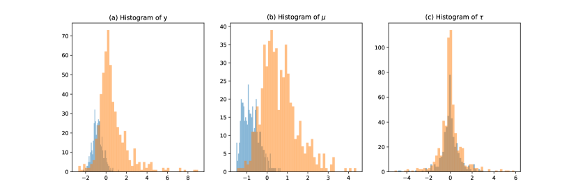
Figure 1: Synthetic data histograms

We calculate three metrics to evaluate and benchmark our method. We consider the average treatment effect (ATE) calculated from the sample and compute mean squared error (MSE) as well as coverage and average interval length. Further, we consider conditional average treatment effect (CATE), averaged over the sample.

First, we show some plots that demonstrate the quality of our fit of the response, shown in Figure 2.

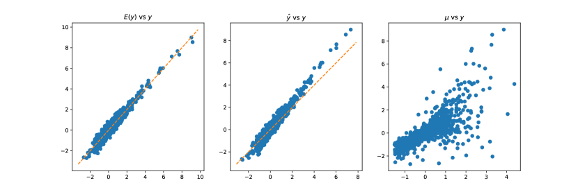
Figure 2: The middle plot compares fitted reposes $\hat{y}$ and simulated ones $y$. Left plot compares the simulated $y$ vs the noseless values $E(y)$. Right plot shows $y$ vs $\mu$.

We use neural networks as building blocks of our model. Each layer of a neural network is a function of the form

$$f(x;W,l)=h(Wx),~{}x\in\Re^{d},~{}W\in\Re^{d\times l},$$

where $h$ is a nonlinear univariate function, such as ReLU, applied element-wise to $x$, and $l$ is the number of neurons in the layer. We use the following architecture for the response surface. We start by calculating a cosine embedding of of the quantile $q$

$$s_{i}=\cos(i\pi q),~{}i=1,\ldots,32$$

$$s= f(s;W_{1},32)$$

$$\tilde{\pi}= f(x;W_{2},8)$$

$$\hat{\pi}= f(\tilde{\pi};W_{3},32)$$

$$\hat{z}= \sigma(\hat{\pi})$$

$$\mu= q\circ f([x,\tilde{\pi}];W_{3},32)$$

$$\tau= q\circ f(x;W_{5},32)$$

$$\hat{y}= W_{6}(\mu+\tau\circ\hat{z}),~{}W_{6}\in\Re^{32\times 2}.$$

Here $\circ$ stands for element-wise multiplication. Our model generates a two-dimensional output $\hat{y}$, first element is the mean response and the second is the quantile response. We use the following loss function to jointly estimate the components of our model

$$q\sim U(0,1)$$

$$l_{z}= (1/n)\sum_{i=1}^{n}z_{i}\log\hat{z}_{i}+(1-z_{i})\log(1-\hat{z}_{i})$$

$$e_{i}= y_{i}-\hat{y}_{i}$$

$$l_{\mathrm{MSE}}= (1/n)\sum_{i=1}^{n}e_{i1}^{2}$$

$$l_{q}= (1/n)\sum_{i=1}^{n}\max(qe_{i2},(q-1)e_{i2})$$

$$l= w_{1}l_{z}+w_{2}l_{q}+w_{3}l_{\mathrm{MSE}}$$

We add a constraint to the loss function to prevent the quantiles to cross, specifically our constraints are

$$\begin{cases}\hat{y}(\tau)<y,&\mbox{ when }\tau<0.5\\ \hat{y}(\tau)>y,&\mbox{ when }\tau>0.5.\end{cases}$$

We add this constraint as a penalty term to the loss function.

Figure 3: Histogram of fitted propensity scores $\hat{\pi}(x)$

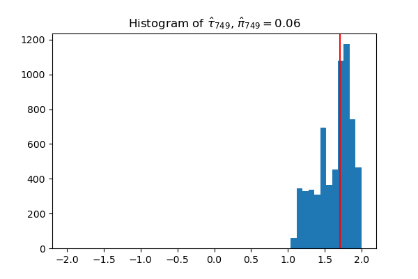
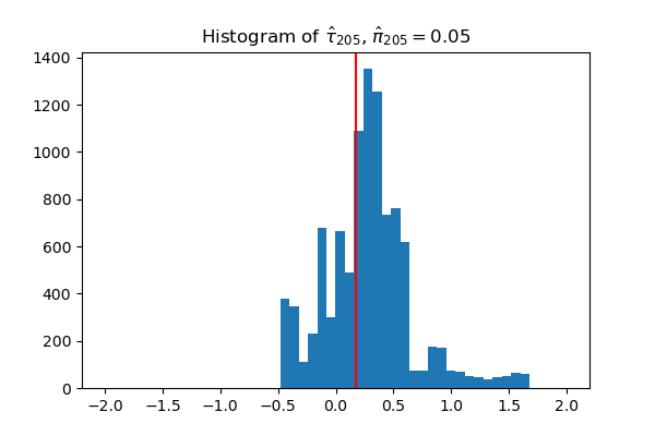
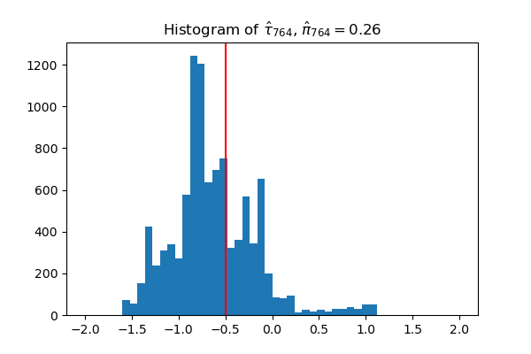
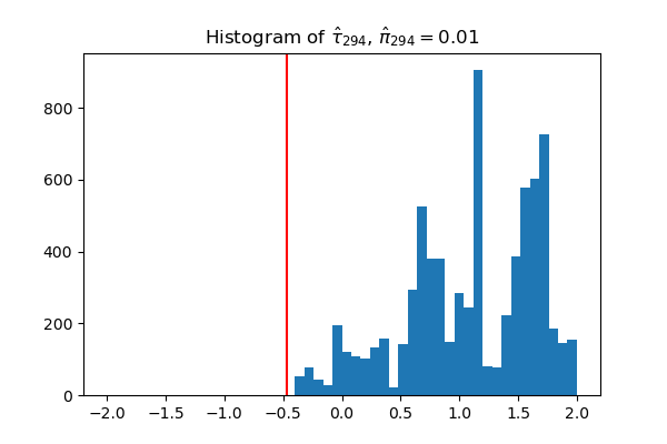
Figure 4: Histogram of posterior values of treatment effect $\tau$ for randomly selected units that were assigned no treatment ($z=0$).

Figure 4 shows the posterior distribution of the treatment effect $\tau$ for randomly selected units that were assigned no treatment ($z=0$). The vertical red line is the true value of the treatment effect. The posterior distribution of $\tau$ is also very tight, which is consistent with the fact that the control group is large.

5 Discussion

Generative methods differ from traditional simulation based tools in that they use a large training data set to infer predictive mappings rather than density methods The main tool is high-dimensional nonlinear nonparametric regression using deep neural networks. Inference for the observed data is then evaluation of the network and is therefore an interpolation approach to inference. There are many avenues for future research. Given wide applicability of simulation in econometrics models, designing architectures for specific problems is a a paramount interest.

References

- Antonelli et al. (2022) Joseph Antonelli, Georgia Papadogeorgou, and Francesca Dominici. Causal inference in high dimensions: A marriage between Bayesian modeling and good frequentist properties. Biometrics, 78(1):100–114, March 2022.
- Athey et al. (2019) Susan Athey, Julie Tibshirani, and Stefan Wager. Generalized random forests. The Annals of Statistics, 47(2):1148–1178, April 2019.
- Banerjee et al. (2020) Abhijit Banerjee, Esther Duflo, and Nancy Qian. On the road: Access to transportation infrastructure and economic growth in China. Journal of Development Economics, 145:102442, 2020.
- Bernardo (1979) Jose M. Bernardo. Expected Information as Expected Utility. The Annals of Statistics, 7(3), May 1979.
- Bhadra et al. (2021) Anindya Bhadra, Jyotishka Datta, Nick Polson, Vadim Sokolov, and Jianeng Xu. Merging two cultures: deep and statistical learning. arXiv preprint arXiv:2110.11561, 2021.
- Dawid (2000) A. P. Dawid. Causal Inference without Counterfactuals. Journal of the American Statistical Association, 95(450):407–424, June 2000.
- Duflo et al. (2007) Esther Duflo, Rachel Glennerster, and Michael Kremer. Using Randomization in Development Economics Research: A Toolkit. In T. Paul Schultz and John A. Strauss, editors, Handbook of Development Economics, volume 4, pages 3895–3962. Elsevier, January 2007.
- Gallant and White (1988) Gallant and White. There exists a neural network that does not make avoidable mistakes. In IEEE 1988 International Conference on Neural Networks, pages 657–664 vol.1, July 1988.
- Hahn (1998a) Jinyong Hahn. On the Role of the Propensity Score in Efficient Semiparametric Estimation of Average Treatment Effects. Econometrica, 66(2):315–331, 1998a.
- Hahn (1998b) Jinyong Hahn. On the Role of the Propensity Score in Efficient Semiparametric Estimation of Average Treatment Effects. Econometrica, 66(2):315–331, 1998b.
- Hahn et al. (2018) P. Richard Hahn, Carlos M. Carvalho, David Puelz, and Jingyu He. Regularization and Confounding in Linear Regression for Treatment Effect Estimation. Bayesian Analysis, 13(1):163–182, March 2018.
- Hahn et al. (2020) P. Richard Hahn, Jared S. Murray, and Carlos M. Carvalho. Bayesian Regression Tree Models for Causal Inference: Regularization, Confounding, and Heterogeneous Effects (with Discussion). Bayesian Analysis, 15(3):965–1056, September 2020.
- Hill and McCulloch (2007) Jennifer Hill and Robert McCulloch. Bayesian Nonparametric Modeling for Causal Inference. Technical report, June 2007.
- Hill (2011) Jennifer L. Hill. Bayesian Nonparametric Modeling for Causal Inference. Journal of Computational and Graphical Statistics, 20(1):217–240, January 2011.
- Hirano et al. (2003) Keisuke Hirano, Guido W. Imbens, and Geert Ridder. Efficient Estimation of Average Treatment Effects Using the Estimated Propensity Score. Econometrica, 71(4):1161–1189, 2003.
- Holland (1986) Paul W. Holland. Statistics and Causal Inference. Journal of the American Statistical Association, 81(396):945–960, 1986.
- Imbens and Rubin (2015) Guido W. Imbens and Donald B. Rubin. Causal Inference for Statistics, Social, and Biomedical Sciences: An Introduction. https://www.cambridge.org/core/books/causal-inference-for-statistics-social-and-biomedical-sciences/71126BE90C58F1A431FE9B2DD07938AB, April 2015.
- Jiang et al. (2017) Bai Jiang, Tung-Yu Wu, Charles Zheng, and Wing H. Wong. Learning Summary Statistic For Approximate Bayesian Computation Via Deep Neural Network. Statistica Sinica, 27(4):1595–1618, 2017.
- Lasserre et al. (2006) Julia A Lasserre, Christopher M Bishop, and Thomas P Minka. Principled hybrids of generative and discriminative models. In 2006 IEEE Computer Society Conference on Computer Vision and Pattern Recognition (CVPR’06), volume 1, pages 87–94. IEEE, 2006.
- McCullagh (2022) Peter McCullagh. Ten Projects in Applied Statistics. Springer Series in Statistics. Springer International Publishing, Cham, 2022. ISBN 978-3-031-14274-1 978-3-031-14275-8.
- Nareklishvili et al. (2022a) Maria Nareklishvili, Nicholas Polson, and Vadim Sokolov. Deep partial least squares for iv regression. arXiv preprint arXiv:2207.02612, 2022a.
- Nareklishvili et al. (2022b) Maria Nareklishvili, Nicholas Polson, and Vadim Sokolov. Feature selection for personalized policy analysis. arXiv preprint arXiv:2301.00251, 2022b.
- Nareklishvili et al. (2023) Maria Nareklishvili, Nicholas Polson, and Vadim Sokolov. Deep partial least squares for instrumental variable regression. Applied Stochastic Models in Business and Industry, 2023.
- Pearl (2009) Judea Pearl. Causality. Cambridge university press, 2009.
- Polson et al. (2021) Nicholas Polson, Vadim Sokolov, and Jianeng Xu. Deep learning partial least squares. arXiv preprint arXiv:2106.14085, 2021.
- Polson and Sokolov (2023) Nicholas G Polson and Vadim Sokolov. Generative ai for bayesian computation. arXiv preprint arXiv:2305.14972, 2023.
- Puelz et al. (2022) David Puelz, Guillaume Basse, Avi Feller, and Panos Toulis. A Graph-Theoretic Approach to Randomization Tests of Causal Effects under General Interference. Journal of the Royal Statistical Society Series B: Statistical Methodology, 84(1):174–204, February 2022.
- Rosenbaum and Rubin (1983) Paul R. Rosenbaum and Donald B. Rubin. The central role of the propensity score in observational studies for causal effects. Biometrika, 70(1):41–55, April 1983.
- Rubin (1974) Donald B. Rubin. Estimating causal effects of treatments in randomized and nonrandomized studies. Journal of Educational Psychology, 66(5):688–701, October 1974.
- Rubin and Waterman (2006) Donald B. Rubin and Richard P. Waterman. Estimating the Causal Effects of Marketing Interventions Using Propensity Score Methodology. Statistical Science, 21(2):206–222, 2006.
- Sohl-Dickstein et al. (2015) Jascha Sohl-Dickstein, Eric A. Weiss, Niru Maheswaranathan, and Surya Ganguli. Deep Unsupervised Learning using Nonequilibrium Thermodynamics, November 2015.
- Splawa-Neyman et al. (1990) Jerzy Splawa-Neyman, D. M. Dabrowska, and T. P. Speed. On the Application of Probability Theory to Agricultural Experiments. Essay on Principles. Section 9. Statistical Science, 5(4), November 1990.
- Stephens et al. (2023) David A. Stephens, Widemberg S. Nobre, Erica E. M. Moodie, and Alexandra M. Schmidt. Causal Inference Under Mis-Specification: Adjustment Based on the Propensity Score. Bayesian Analysis, -1(-1):1–46, January 2023.
- Tian and Pearl (2013) Jin Tian and Judea Pearl. Probabilities of Causation: Bounds and Identification, January 2013.
- Vasilescu (2022) M. Alex O. Vasilescu. Causal Deep Learning: Causal Capsules and Tensor Transformers, December 2022.
- Wager and Athey (2018) Stefan Wager and Susan Athey. Estimation and Inference of Heterogeneous Treatment Effects using Random Forests. Journal of the American Statistical Association, 113(523):1228–1242, July 2018.
- Wang et al. (2022) Yuexi Wang, Nicholas Polson, and Vadim O Sokolov. Data augmentation for bayesian deep learning. Bayesian Analysis, 1(1):1–29, 2022.
- White (1989) Halbert White. Some Asymptotic Results for Learning in Single Hidden-Layer Feedforward Network Models. Journal of the American Statistical Association, 84(408):1003–1013, December 1989.
- Xu et al. (2018) Dandan Xu, Michael J. Daniels, and Almut G. Winterstein. A Bayesian nonparametric approach to causal inference on quantiles: A Bayesian Nonparametric Approach to Causal Inference on Quantiles. Biometrics, 74(3):986–996, September 2018.