Linear regression for Poisson count data:
A new semi–analytical method with applications to COVID-19 events

Abstract

This paper presents the application of a new semi—analytical method of linear regression for Poisson count data to COVID-19 events. The regression is based on the Bonamente and Spence (2022) maximum–likelihood solution for the best–fit parameters, and this paper introduces a simple analytical solution for the covariance matrix that completes the problem of linear regression with Poisson data.

The analytical nature for both parameter estimates and their covariance matrix is made possible by a convenient factorization of the linear model proposed by J. Scargle (2013). The method makes use of the asymptotic properties of the Fisher information matrix, whose inverse provides the covariance matrix. The combination of simple analytical methods to obtain both the maximum–likelihood estimates of the parameters, and their covariance matrix, constitute a new and convenient method for the linear regression of Poisson–distributed count data, which are of common occurrence across a variety of fields.

A comparison between this new linear regression method and two alternative methods often used for the regression of count data — the ordinary least–square regression and the $\chi^{2}$ regression – is provided with the application of these methods to the analysis of recent COVID–19 count data. The paper also discusses the relative advantages and disadvantages among these methods for the linear regression of Poisson count data.

,

1 Introduction

Integer–count data based on the Poisson distribution are quite common in real–life applications, from S.-D. Poisson’s use of his name–sake distribution for the study of civil and criminal cases (Poisson, 1837), Lord Rutherford’s characterization of the rate of decay of radioactive isotopes (Rutherford, Chadwick and Ellis, 1920) and R.D. Clarke’s application to the number of bombs that fell in London during World War II (Clarke, 1946), to the distribution of low–count political events (King, 1988), such as the number of seats lost by the president’s party in a mid–term election (Campbell, 1985), or the study of mutations in bacteria (Luria and Delbrück, 1943). The common occurrence of the Poisson distribution lies primarily with its association to the Poisson process, whereby this distribution describes the probability of occurrence of events — e.g., in a period of time or for a spatial region — from a process with a fixed rate of occurrence (e.g., Ross, 2003). Among the data analysis methods for Poisson–based count data, the linear regression plays a fundamental role, given that the linear model is arguably the simplest model that enforces a correlation between the indepedendent variables (or regressors) and the dependent measured variables.

The maximum–likelihood estimate of a two–parameter linear model for integer–valued count data can be accomplished with the use of the Poisson log–likelihood, also known as the Cash or ${C}$ statistic  (Cash, 1979). Despite its common occurrence, it has been elusive to find a simple analytical expression for the maximum–likelihood estimates of the parameters for the Poisson regression (see, e.g., Sect. 2.2 of Cameron and Trivedi 2013). This restriction has resulted in a limited use of the maximum–likelihood method for the regression of count data. This is in contrast to the simple analytical solutions that are available for the ordinary least–squares (OLS) regression for data with equal variances (i.e, homoskedastic data) or with different variances (i.e, heteroskedastic data), and for the regression with the $\chi^{2}$ statistic, which is a maximum–likelihood method for heteroskedastic data of common use for normally–distributed data (e.g. Greenwood and Nikulin, 1996). Such simple analytical solutions, which also extend to the more general multiple linear regression with more than two adjustable parameters (e.g., see Bonamente 2022 for a review), are now a standard of practice for the linear regression. Their use is in fact so widespread that it is not uncommon to see $\chi^{2}$–based methods of regression even for Poisson count data for which the method is not justified, or rather it is known to lead to known biases that have been documented as early as Lewis and Burke (1949), and more recently by Kelly (2007) and Bonamente (2020).

Motivated by the need to provide a simple maximum–likelihood method for the linear regression of count data (sometimes also referred to as cross–section data) that explicitly accounts for the Poisson distribution of the measurements, in Bonamente and Spence (2022) we have reported the first semi–analytical solution for the parameters of the linear regression with the Poisson–based ${C}$ statistic. In this paper we continue the investigation of the same problem, and report a new analytical solution for the covariance matrix of the two model parameters, based on the Fisher information matrix (Fisher, 1922). The combination of the new results presented in this paper and those provided in Bonamente and Spence (2022) thus provide a complete treatment of the maximum–likelihood linear regression with Poisson–distributed count data. The availability of these new analytical methods for the linear regression of count data therefore represents a key step towards a wider use of an unbiased method of regression for such integer–count data, without the need to resort to either numerical solutions or the use of alternative and less accurate methods, such as those based on least–squares or the $\chi^{2}$ statistic.

There are alternatives to the modelling of count data with the simple one–parameter Poisson distribution considered in this paper. One of the key limitations of the Poisson regression is the inability to properly model overdispersed data (see, e.g., discussion in Chapter 3 of Cameron and Trivedi (2013)). For such overdispersed data, other data models such as the negative binomial distribution can be used (Hilbe, 2014). Alternatively, the standard Poisson maximum–likelihood regression can be modified to a quasi–MLE regression with empirical variance functions that reflect the overdispersion (e.g. Cameron and Trivedi, 1986), also used in the generalized linear model (GLM) literature (e.g. McCullagh and Nelder, 1989). Nonetheless, the simple linear regression of Poisson count data is an essential tool for the data analyst, and the development of simple analytical tools for its application is the subject of this paper.

The paper is structured as follows: Sect. 2 summarizes the model for the regression with count data, which is described in full in Bonamente and Spence (2022); Sect. 3 describes methods to obtain the covariance matrix, with Sect. 3.3 describing the properties of the matrix for the Poisson linear regression under consideration and Sect. 3.4 presenting an alternative method to estimate the covariance matrix based on the error propagation method. Sect. 4 provides an application of the results to recent COVID–19 data with comparison to the least–squares and $\chi^{2}$ methods. Finally, Sect. 5 contains a discussion and the conclusions.

2 Model for the regression of count data with the ${C}$ statistic

The data under consideration are in the form of independent pairs of measurements $(x_{i},y_{i})$, where $y_{i}$ are Poisson–distributed variables, for $i=1,\dots,N$, and $x_{i}$ are fixed values of the independent variable.

2.1 The Scargle et al. (2013) parameterization of the linear model

A convenient parameterization of the linear model was proposed by Scargle et al. (2013), and it is in the form of

$$f_{S}(x)=\lambda(1+a(x-x_{A})),$$ (1)

where $x_{A}$ is a constant that usually coincides with the beginning of the range of the independent variable $x$, and $\lambda$ and $a$ are the two parameters. This parameterization is thus equivalent to a linear model with overall slope $\lambda\,a$, and intercept $\lambda(1-a\,x_{A})$, yet this factorization has algebraic andvantages when used in the Poisson log–likelihood. The parent mean of the Poisson distribution of the variable $y_{i}$ is then

$$\mu_{i}=f_{S}(x_{i})\,\Delta x_{i},$$ (2)

with $\Delta x_{i}$ the width of the $i$–th bin of data, which is not required to be uniform among the measurements.

2.2 Maximum–likelihood regression

Upon minimization of the logarithm of the Poisson likelihood of the data with model, in Bonamente and Spence (2022) we have shown that the method of maximum likelihood yields two simple equations for the determination of the parameter estimates. The first is a analytical relationship between the two parameters,

$$\lambda(a)=\frac{M}{R\left(1+a\dfrac{R}{2}\right)}$$ (3)

with $M$ the sum of all integer counts $y_{i}$, and $R$ the range of the independent variable, typically chosed to be $R=x_{B}-x_{A}$. This equations enables the determination of $\hat{\lambda}$ from $\hat{a}$. The second is an equation that must be solved to obtain $\hat{a}$, and it is conveniently cast as the zero of a function $F(a)$,

$$F(a)=1+\dfrac{R}{2}\left(a-\dfrac{M}{g(a)}\right)=0,\,\text{ with }g(a)=\sum_{i=1}^{N}y_{i}\dfrac{(x_{i}-x_{A})}{1+a(x_{i}-x_{A})}.$$ (4)

In general, solution of (4) to obtain the estimate $\hat{a}$ can be obtained numerically. The inherently analytical method leading to (3) and (4), and the need for a numerical solution of the latter, constitute this new semi–analytical method for the linear regression of Poisson count data. The properties of the two functions $F(a)$ and $g(a)$ are described in detail in Bonamente and Spence (2022), and the key properties are reported in the following.

2.3 Identification of points of singularity and zeros of $g(a)$

It is immediate to identify the $n$ points of singularity of $g(a)$ and its zeros, using the property that $g^{\prime}(a)<0$ between points of singularity. Since it is also true that $F^{\prime}(a)<0$ between its points of singularity, which are the zeros of $g(a)$, the $n-1$ zeros of $F(a)$ can be easily found because of the continuity of the function between singularities. In particular, the acceptable solution — defined as the pair of best–fit parameters $(\hat{a},\hat{\lambda})$ that gives a non–negative model throughout its support, as required by the counting nature of the Poisson distribution — is either the first or the last zero, according to the asymptotic value of the function $F(a)$ for $a\to\pm\infty$. The acceptable solution $\hat{a}$ can therefore be found with elementary numerical methods from the equation $F(a)=0$.

2.4 Applicability of model to data with gaps

Both equations (3) and (4) apply to data with arbitrary bin size. Moreover, when there are gaps in the data, defined as intervals of the $x$ variable without measurements, the two equations are modified with the introduction of a modified range $R_{m}$ defined as

$$R_{m}=\dfrac{R^{2}-2S_{G}}{R-R_{g}}$$ (5)

where $R_{G}$ is the sum of the ranges $R_{G,j}$ of all the gaps, and $S_{G}$ is a constant defined by

$$S_{G}=\sum_{j=1}^{g}R_{G,j}(x_{G,j}-x_{A})$$

with $x_{G,j}$ the midpoint of the $j$–th gap. The equations are modified to 

$$\begin{cases}F(a)=1+\dfrac{aR_{m}}{2}-\dfrac{MR_{m}}{2g(a)}=0\\[10.0pt] \lambda(a)=\dfrac{M}{R\left(1+a\dfrac{R}{2}\right)-(R_{G}+aS_{G})}\end{cases}$$ (6)

Such modifications for the presence of gaps in the data do not introduce any additional statistical complication to the analysis of either the maximum–likelihood estimates or the covariance matrix. Gaps in the data are quite common in data analysis, for example when a range of wavelengths in the spectrum of an astronomical source is unavailable (e.g., because of detector inefficiencies, as in Ahoranta et al., 2020), or when a time interval for the light–curve of a source is unobserved (e.g. Levine et al., 1996).

The reason for the parameterization of the linear model according to (1) is that the two resulting equations (3) and (4) can be used to identify the maximum–likelihood parameter estimates more easily than for the standard parameterization $a+b\,x$, which leads to two coupled non–linear equations instead (as noted, e.g., in Ch. 16 of Bonamente 2022). Moreover, as will be shown in the next section, these equations lead to a very convenient analytical solution for the covariance matrix, which represents the main new result of this paper.

3 Evaluation of the covariance matrix

3.1 General properties of the covariance matrix

The maximum–likelihood estimators of the linear model parameters $\hat{\theta}=(\hat{\lambda},\hat{a})$ from Poisson count data are normally distributed, but only in the asymptotic limit of a large number of measurements $N$ (see, e.g., Eadie et al. 1971; Cameron and Trivedi 2013). In this asymptotic limit, the maximum–likelihood estimators are also unbiased and efficient, with their variance reaching the Cramér–Rao lower bound (see, e.g., Rao 1945; Cramer 1946; Amemiya 1985). Within this limit, it is thus possible to approximate the covariance or error matrix of the parameters, defined by

$$\varepsilon=\text{E}[(\hat{\theta}-\theta_{0})(\hat{\theta}-\theta_{0})^{T}],$$

as the inverse of the Fisher information matrix,

$$\hat{\varepsilon}=-\left(\text{E}\left[\dfrac{\partial^{2}\ln\mathscr{L}}{\partial\theta\,\partial\theta^{\prime}}\right]\right)^{-1}_{\theta=\theta_{0}}=-\left(\text{E}\left[\sum_{i=1}^{N}\dfrac{\partial^{2}\ln f(x_{i})}{\partial\theta\,\partial\theta^{\prime}}\right]\right)^{-1}_{\theta=\theta_{0}}.$$ (7)

In this application, $f(x_{i})$ is the Poisson distribution for the measurement at a value $x_{i}$ of the indepedendent variable, with a $\mu_{i}$ parameter given by (2), and the expectation in (7) is taken with respect to this distribution.  In practice, (7) means that the maximum–likelihood estimates of the parameters of the linear model converge in distribution to a normal distribution with the covariance matrix given by (7), or

$$(\hat{\theta}-\theta_{0})\overset{d}{\to}N(0,\hat{\varepsilon}).$$

R. A. Fisher was the first to associate the concept of information with the second derivative — or curvature — of the logarithm of the likelihood Fisher (1922), and similar definitions of information have been derived from this idea (e.g., Shannon and Weaver (1949); Kullback and Leibler (1951); Akaike (1974)). Given that the true parameter values $\theta_{0}$ are unknown, the information matrix is evaluated at $\theta=\hat{\theta}$, in recognition of the fact that the maximum–likelihood estimates are unbiased and thus asymptotically converge to the true–yet–unknown values (e.g., Fisher 1922, Chapter IX of Fisher 1925, or Chapter 33 of Cramer 1946).

3.2 Evaluation of the covariance matrix for the Poisson linear regression with the Scargle et al. (2013) parameterization

The negative of the logarithm of the likelihood, which is related to the ${C}$ statistic by $C=-2\ln\mathscr{L}+\text{const}$, can be written as

$$-\ln\mathscr{L}=\lambda(R-R_{G})+\lambda aS_{1}-M\ln\lambda-\sum_{i=1}^{N}y_{i}\ln(1+a(x_{i}-x_{A})),$$ (8)

where the constant $S_{1}$ is defined by

$$S_{1}=\sum_{i=1}^{N}(x_{i}-x_{A})\Delta x_{i}=\dfrac{R^{2}-2S_{G}}{2},$$ (9)

and the second equation connects $S_{1}$ with the constants defined in Sect. 2, and it is an immediate consequence of the model linearity. The first derivatives are

$$\begin{cases}-\dfrac{\partial\ln\mathscr{L}}{\partial a}=\lambda S_{1}-g(a)\\[10.0pt] -\dfrac{\partial\ln\mathscr{L}}{\partial\lambda}=(R-R_{G})+aS_{1}-\dfrac{M}{\lambda}\end{cases}$$ (10)

which, when set to zero, yield the usual maximum–likelihood estimates described in Sect. 2 and in more detail in Bonamente and Spence (2022). From these, it is immediate to evaluate the second order derivatives and thus obtain

$$-\dfrac{\partial^{2}\ln\mathscr{L}}{\partial\theta\,\partial\theta^{\prime}}=\begin{bmatrix}\dfrac{M}{\lambda^{2}}&S_{1}\\[10.0pt] S_{1}&G(a)\end{bmatrix}$$ (11)

with a new function $G$ defined as

$$G(a)=-\dfrac{\partial g(a)}{\partial a}=\sum_{i=1}^{N}\dfrac{y_{i}(x_{i}-x_{A})^{2}}{(1+a(x_{i}-x_{A}))^{2}}.$$ (12)

The expectation of (11) is immediately calculated with the consideration that

$$\left.\text{E}[y_{i}]\right|_{\hat{\theta}}=\left.\mu_{i}\right|_{\hat{\theta}}=\hat{\lambda}(1+\hat{a}(x_{i}-x_{A}))\Delta x_{i},$$

where $\Delta x_{i}$ is the size of the $i$–th bin of data. Given that all terms in (11) are linear in the measurements $y_{i}$, the expectation is found as

$$-\left.\text{E}\left[\dfrac{\partial^{2}\ln\mathscr{L}}{\partial\theta\,\partial\theta^{\prime}}\right]\right|_{\hat{\theta}}=\begin{bmatrix}\dfrac{(R-R_{G})+\hat{a}S_{1}}{\hat{\lambda}}&S_{1}\\[10.0pt] S_{1}&\hat{\lambda}\,H(\hat{a})\end{bmatrix},$$ (13)

with

$$H(a)=\sum_{i=1}^{N}\dfrac{(x_{i}-x_{A})^{2}}{1+{a}(x_{i}-x_{A})}\Delta x_{i}$$ (14)

defined as a convenient analytical function to describe one of the terms of the information matrix. Notice how the bin size appears explicitly in this function, unlike in the case of the function $g(a)$ in (4), which is independent of the bin size.

With the simple analytical expression available for the second–order derivatives of the logarithm of the likelihood (13), it is finally possible to provide the asymptotic estimate of the covariance matrix as its inverse,

$$\hat{\varepsilon}=\begin{bmatrix}\hat{\sigma}^{2}_{a}&\hat{\sigma}^{2}_{a\,\lambda}\\[5.0pt] \hat{\sigma}^{2}_{a\,\lambda}&\hat{\sigma}^{2}_{\lambda}\end{bmatrix}=\dfrac{1}{\Delta}\begin{bmatrix}\hat{\lambda}\,H(\hat{a})&-S_{1}\\[10.0pt] -S_{1}&\dfrac{(R-R_{G})+\hat{a}S_{1}}{\hat{\lambda}}\end{bmatrix},$$ (15)

with $\Delta$ the determinant of the matrix (13),

$$\Delta=\left((R-R_{G})+\hat{a}S_{1}\right)H(\hat{a})-S_{1}^{2}.$$

This simple analytical form for the covariance matrix of the maximum–likelihood estimates for the linear regression to Poisson data is the main result of this paper. Its properties are analyzed in the following section.

3.3 Properties of the covariance matrix

Basic results on the sign of the terms in the covariance matrix (15) are provided in this section. First, it is necessary to recall the definition of acceptability of the estimates of the model parameters as values that ensure a non–negative parent Poisson mean, which was briefly introduced in Sect. 2. Acceptable solutions for $\hat{a}$ and $\hat{\lambda}$ require that the quantities

$$\hat{\lambda}(1+\hat{a}(x_{i}-x_{A}))$$

are all non–negative. This results in values of the two parameters to be found in two possible ranges, namely (a) for $\hat{a}\leq-2/\Delta x_{1}$, where $\hat{\lambda}<0$, or (b) for $\hat{a}>-1/(R-\Delta x_{N}/2)$, where $\hat{\lambda}>0$ (see Lemma 5.2 of Bonamente and Spence 2022 for a proof). In the following, it is assumed that $x_{A}$ is the beginning of the range of the independent variable $x$.

Lemma 3.1 (Sign of the determinant $\Delta$).

The determinant $\Delta$ in (15) is positive definite for all acceptable solutions of the regression coefficients.

Proof.

The determinant can be written as

$$\Delta=\sum_{i=1}^{N}\dfrac{(x_{i}-x_{A})^{2}}{1+\hat{a}(x_{i}-x_{A})}\Delta x_{i}\cdot\sum_{i=1}^{N}(1+\hat{a}(x_{i}-x_{A}))\Delta x_{i}-\left(\sum_{i=1}^{N}(x_{i}-x_{A})\Delta x_{i}\right)^{2}.$$

This is in the form

$$\Delta=\sum_{i=1}^{N}\dfrac{r_{i}^{2}}{s_{i}}\cdot\sum_{i=1}^{N}s_{i}-\left(\sum_{i=1}^{N}r_{i}\right)^{2}$$

with $r_{i}=(x_{i}-x_{A})\Delta x_{i}$ and $s_{i}=(1+\hat{a}(x_{i}-x_{A}))\Delta x_{i}$. Notice that the terms $s_{i}$ are either all positive or all negative, therefore making it such that one can use $|s_{i}|$ in their place in the previous equation,

$$\Delta=\sum_{i=1}^{N}\dfrac{r_{i}^{2}}{|s_{i}|}\cdot\sum_{i=1}^{N}|s_{i}|-\left(\sum_{i=1}^{N}r_{i}\right)^{2}.$$

With the substitution $a_{i}=r_{i}/\sqrt{|s_{i}|}$ and $b_{i}=\sqrt{|s_{i}|}$, the determinant becomes

$$\Delta=\sum_{i=1}^{N}a_{i}^{2}\cdot\sum_{i=1}^{N}b_{i}^{2}-\left(\sum_{i=1}^{N}a_{i}b_{i}\right)^{2}\geq 0,$$

according to the Cauchy–Schwartz inequality. ∎

It is also possible to show that the variances of $\hat{a}$ and $\hat{\lambda}$ have the proper sign, and that the covariance between them is negative.

Lemma 3.2 (Signs of variance and covariance terms).

The diagonal terms in the covariance matrix (15) are positive, and the off–diagonal terms are negative, for all acceptable solutions of the linear regression coefficients.

Proof.

The term $S_{1}$ is positive according to its definition (9), and therefore the covariance is always negative.

According to (14), the variance of the estimate $\hat{a}$ is

$$\hat{\sigma}^{2}_{a}=\dfrac{\hat{\lambda}H(\hat{a})}{\Delta}=\dfrac{\hat{\lambda}}{\Delta}\sum_{i=1}^{N}\dfrac{(x_{i}-x_{A})^{2}}{1+{a}(x_{i}-x_{A})}\Delta x_{i}.$$

Given the discussion at the beginning of this section, $\hat{\lambda}$ and each of the terms $1+\hat{a}(x_{i}-x_{A})$ must have the same sign for acceptable values of the regression coefficients. The variance is therefore always positive, as it should.

For the same reasons, the variance of $\hat{\lambda}$ is immediately shown to have the proper sign,

$$\hat{\sigma}^{2}_{\lambda}=\dfrac{1}{\Delta\hat{\lambda}}\left((R-R_{G})+\hat{a}S_{1}\right)=\dfrac{1}{\Delta}\dfrac{\sum_{i=1}^{N}(1+\hat{a}(x_{i}-x_{A}))\Delta x_{i}}{\hat{\lambda}}\geq 0.$$

Finally, the negative sign of the covariance term is an immediate consequence of the definition of $S_{1}$ from (9). ∎

Al alternative approach to achieve a non–negative Poisson mean for all values of the model parameters would be to perform an exponential transform, so that the expectations for the Poisson–distributed mesurements is, for example, of the type $\mu_{i}=\exp\left({a+b\,x_{i}}\right)$ (see, e.g. Sect. 2.2 of Cameron and Trivedi 2013). In practice, this corresponds to a linear model for the logarithm of the means, $\log\mu_{i}=a+b\,x_{i}$. Although this transformation does indeed provide a Poisson mean $\mu_{i}$ that is always non–negative, the model is no longer linear between $x$ and $y$, and therefore unsuitable for those cases where a linear relationship is required, e.g., because of the physical nature of the two variables. Moreover, even with this exponential transformation, the maximum–likelihood method of regression for Poisson data does not have an analytical solution with the usual parameterization of the linear model Cameron and Trivedi (2013).

3.4 An alternative approximation for the covariance matrix

A different analytical approximation for the covariance matrix of the coefficients of the linear regression can be given using the error propagation method, also known as the delta method (e.g. Bevington and Robinson, 2003; Cameron and Trivedi, 2013). The method consists of treating the parameters as a function of the independent measurements, $\theta_{j}=\theta_{j}(y_{k})$, and approximating the variances and covariances with the first–order terms of their Taylor series,

$$\hat{\sigma}^{2}_{\theta_{i}\,\theta_{j}}\simeq\sum_{k=1}^{N}\left.\left(\dfrac{\partial\theta_{i}}{\partial y_{k}}\right)\right|_{\hat{\theta}}\left.\left(\dfrac{\partial\theta_{j}}{\partial y_{k}}\right)\right|_{\hat{\theta}}\sigma^{2}_{k},$$ (16)

where $\sigma^{2}_{k}$ is an estimate of the variance of the measurement $y_{k}$. The regression model described in Sect. 2 does not lead to best–fit parameters $\hat{\theta}$ that are described as a function of the measurements in a closed form. Nonetheless, it is possible to take the derivatives of both (3) and (4), or more generally (6), with respect to $y_{j}$ to obtain the derivatives $\partial\theta_{i}/\partial y_{k}$ as follows.

Start with

$$\lambda R\left(1+a\dfrac{R}{2}\right)-\lambda(R_{G}+aS_{G})=M$$

which is the most general equation to obtain $\hat{a}$ in the presence of gaps in the data and of non–uniform binning. The equation can be brought in a simpler form as

$$\lambda(R-R_{G})+a\lambda\left(\dfrac{R^{2}}{2}-S_{G}\right)=\sum_{i=1}^{N}y_{i}$$

leading to

$$\dfrac{\partial\lambda}{\partial y_{j}}\left(R-R_{G}+a\left(\dfrac{R^{2}}{2}-S_{G}\right)\right)+\dfrac{\partial a}{\partial y_{j}}\lambda\left(\dfrac{R^{2}}{2}-S_{G}\right)=1$$

and therefore

$$\dfrac{\partial\lambda}{\partial y_{j}}=\dfrac{1-\lambda\left(\dfrac{R^{2}}{2}-S_{G}\right)\dfrac{\partial a}{\partial y_{j}}}{R-R_{G}+a\left(\dfrac{R^{2}}{2}-S_{G}\right)}.$$ (17)

Alternatively, this partial derivative can be expressed in terms of $a$ alone as

$$\dfrac{\partial\lambda}{\partial y_{j}}=\dfrac{R-R_{G}+\left(\dfrac{R^{2}}{2}-S_{G}\right)\left(a-M\dfrac{\partial a}{\partial y_{j}}\right)}{\left(R-R_{G}+a\left(\dfrac{R^{2}}{2}-S_{G}\right)\right)^{2}},$$ (18)

where the correction for the presence of gaps in the data is in the constants $R_{G}$ and $S_{G}$, both of which become null when the data spans a continous range between $x_{A}$ and $x_{B}$, with $R=x_{B}-x_{A}$.

A similar procedure yields the partial derivatives of $a$ from

$$\left(a+\dfrac{2}{R_{m}}\right)g(a)=M,$$

which is the general expression corresponding to the equation $F(a)=0$ needed to find $\hat{a}$. The equation can be written in a more convenient way as

$$\sum_{i=1}^{N}\dfrac{y_{i}\left(2/R_{m}(x_{i}-x_{A})-1\right)}{1+a(x_{i}-x_{A})}=0$$

and from this, taking the derivative with respect to $y_{j}$,

$$\dfrac{\partial a}{\partial y_{j}}=\dfrac{1-2/R_{m}(x_{j}-x_{A})}{1+a(x_{j}-x_{A})}\cdot\dfrac{1}{g_{2}(a)-2/R_{m}G(a)},$$ (19)

with the aid of a new function defined by

$$g_{2}(a)=\sum_{i=1}^{N}\dfrac{y_{i}(x_{i}-x_{A})}{(1+a(x_{i}-x_{A}))^{2}}.$$ (20)

The result is proven by noting that, in taking the total differential of the term in the sum for $i=j$, there is an extra term due to the presence of the random variable $y_{j}$.

The partial derivatives in (18) and (19) can now be used in (16) to provide an estimate of the covariance matrix from the error propagation method. The variance $\sigma^{2}_{k}$ of the measurement $y_{k}$ can be estimated as either the measurement $y_{k}$ itself, or as the best–fit model $\hat{\mu}_{k}=\text{E}[y_{k}/\hat{\theta}]=\hat{\lambda}(1+\hat{a}(x_{k}-x_{A}))\Delta x_{k}$. In the application provided below in Sect. 4, the parent expectation $\hat{\mu}_{k}$ is used for the numerical result.

4 Application to COVID–19 data

The daily number of deaths caused by the COVID–19 pandemic in the United States provides an example of count data that can be analyzed with the linear regression model presented in this paper. The data are obtained from the New York Times (New York Times, 2021), and they are reported in Table 1.  These data follow the data model of Sect. 2, whereby the number of events are collected in a time interval with a uniform size of length $\Delta x=~{}1$ day, and the measurements in the column ‘Number of events’ are independent of one another.

Table 1: Daily number of events (deaths) reported at the beginning of the pandemic. Data are from New York Times (2021). Day 0 is February 28, 2020, the day prior to the first reported death, which occurred on February 29, 2020.

Day	Number of events	Cumulative
0	0	0
1	1	1
2	2	3
3	3	6
4	4	10
5	2	12
6	0	12
7	3	15
8	4	19
9	3	22
10	4	26
11	5	31
12	6	37
13	6	43
14	7	50
15	10	60
16	8	68
17	23	91
18	26	117
19	45	162
…

This section presents two sets of linear regression to these data with the ${C}$ statistic, to illustrate the novel method of analysis described in this paper and in Bonamente and Spence (2022). It also presents the comparison with two popular regression methods, the ordinary least squares regression and the fit based on the $\chi^{2}$ statistic. The comparison among these methods is used to illustrate the advantages of the new method of linear regression for Poisson data, and to discuss assumptions and limitations of the different methods.

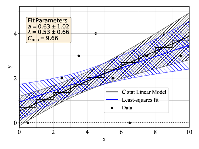
Figure 1: Linear regressions to days 0-9 of the COVID-19 data of Table 1. The black curves correspond to the linear regression with the ${C}$ statistic, and the blue curves for the ordinary least–squares regression.

4.1 Fit to days 0–9 with uniform binning

For this application, the data for days 0 (day prior to first case recorded) through 9 from Table 1 are fit to the linear model, with a total of $N=10$ data points.

4.1.1 The maximum–likelihood parameter estimates

The best–fit model according to (1) is shown in Figure 1 as the black line, with the step–wise continuous black line indicating the best–fit model $\hat{\mu}_{i}$. The two lines intersect because the data are collected over bins with unit size ($\Delta x=1$).

The method of maximum–likelihood regression (see Sect. 2) makes use of two functions $g(a)$ and $F(a)$ that are reported in Figure 2.

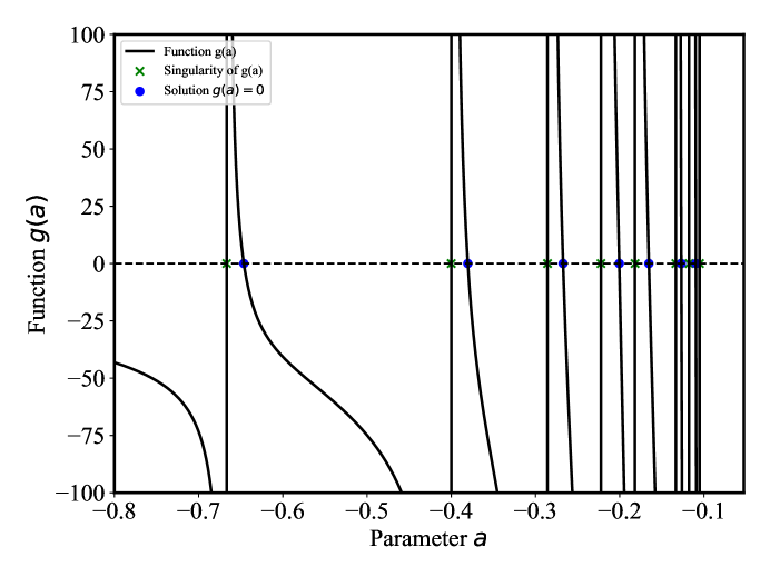
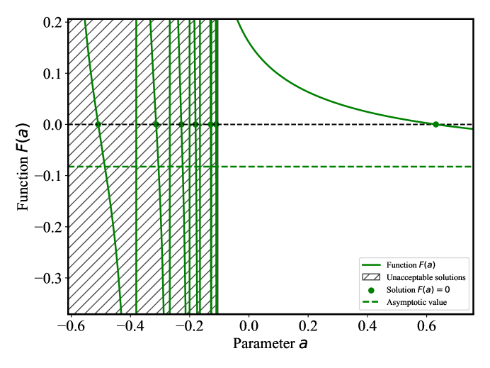
Figure 2: Functions $g(a)$ and $F(a)$ used for the Poisson regression, see (4).

In this application, there is a total of $M=22$ counts for $N=10$ bins and $n=8$ unique non–zero bins. According to (4), this results in $n=8$ points of singularity for $g(a)$ marked as green crosses in Figure 2, and $n-1=7$ roots or zeros of $g(a)$ marked as blue dots between consecutive singularities, with $g^{\prime}(a)<0$ in each interval. The roots of $g(a)$ are also points of singularity for $F(a)$, whose zero(s) are the estimates of the parameter $a$. Of the $n-2=6$ such solutions, only the last one is acceptable, i.e., it is the only value $\hat{a}$ that gives a non–negative model throughout its support, as required for Poisson counts (see Sect. 5 of Bonamente and Spence 2022). Having identified the last singularity of $F(a)$ as the last zero of $g(a)$, the acceptable solution $\hat{a}$ is marked as the rightmost green dot in Figure 2.

It is clear that it is not necessary to identify and calculate all the roots of $g(a)$ in order to determine $\hat{a}$, but just the last one between the last two singularities of $g(a)$. The computational burden is therefore very limited, even for data with a large number of events. Figure 2 report all points of sngularities and the zeros for both $g(a)$ and $F(a)$ only for illustration purposes.

4.1.2 The covariance matrix

The error matrix evaluated according to (15) is

$$\hat{\varepsilon}=\begin{bmatrix}0.346&-0.665\\ -0.665&1.044\end{bmatrix}$$

with the estimated standard deviations of the parameters also reported in the figure, for estimated parameters $\hat{a}=0.63\pm 1.02$ and $\hat{\lambda}=0.53\pm 0.66$.

4.1.3 The log–likelihood or $C$ statistic

Moreover, the fit statistic is evaluated according to

$$C_{\mathrm{min}}=\sum_{i=1}^{N}(\hat{\mu}_{i}-y_{i}+y_{i}\ln\left(y_{i}/\hat{\mu}_{i}\right)),$$ (21)

as reported in Equation 3 of Bonamente and Spence (2022). Hypothesis testing with the ${C}$ statistic requires the evaluation of critical values of its distribution, which is known only in the asymptotic limits of a large number of measurements $N$ and for large parent means, when $C_{\mathrm{min}}$ is approximately distributed as $\chi^{2}(N-m)$ (see, e.g., Lampton, Margon and Bowyer, 1976; Bonamente, 2022), with $m=2$ adjustable parameters. Although a detailed discussion of the method of hypothesis testing with the ${C}$ statistic goes beyond the scope of this paper, it is nonetheless useful to provide a brief description of its application for this example, since hypothesis testing is an integral part of the overall regression. In the present example of small Poisson means, the approximation of $C_{\mathrm{min}}$ with a $\chi^{2}(N-m)$ distribution is not accurate, and in Bonamente (2020) we proposed an approximate method to estimate critical values that applies also to the low–mean case. The method consists of using the parent mean and variance of each term in (21) in place of the mean and variance of a $\chi^{2}(1)$ distribution (which are respectively 1 and 2), and use the central limit theorem to ensure an approximately normal distribution for the statistic. Following this method, the critical value of the $C_{\mathrm{min}}$ distribution for $N-m=8$ degrees of freedom is 13.6 (compared to a corresponding critical value of 13.4 for the $\chi^{2}(8)$ distribution), and therefore these data are consistent with the null hypothesis of a linear model, at the 90% confidence level. Notice how both the parameter estimation and the goodness–of–fit statistic naturally account for measurements with zero counts, such as bins 0 and 6.

4.1.4 The confidence band

The grey hatched band associated with the best–fit model highlights another strength of the availability of the error matrix for the ${C}$ statistic regression, which makes it is possible to estimate the variance of any function of the model parameters. In particular, it is often useful to estimate the variance of the expectation of the $f_{S}(x)$ function for a fixed value of the independent variable $x$, i.e.,

$$\hat{f}_{S}(x)=\text{E}[f_{S}(x)/x,\hat{\theta}]=\hat{\lambda}(1+\hat{a}(1-x)),$$

or, equivalently, for the expectation of the number of counts in a bin centered at $x$ and with arbitrary bin size,

$$\hat{y}_{x}=\text{E}[y/x,\hat{\theta}]=\hat{\lambda}(1+\hat{a}(1-x))\,\Delta x,$$

where $x$ is any value of the regressor variable, not limited to the values $x_{i}$. The variance of the variable $\hat{y}_{x}$ is represented by the variance of $y$ values along a vertical line, for a given $x$. The range $\hat{y}_{x}\pm\sigma_{y_{x}}$ is usually referred to as the confidence band of the best–fit model, and is represented by the grey hatched region in Fig. 1. The variance $\sigma^{2}_{y_{x}}$ is obtained by the error–propagation method, with

$$\hat{\sigma}^{2}_{y_{x}}=\hat{\sigma}^{2}_{\lambda}\left.\left(\dfrac{\partial y_{x}}{\partial\lambda}\right)^{2}\right|_{\hat{\theta}}+\hat{\sigma}^{2}_{a}\left.\left(\dfrac{\partial y_{x}}{\partial a}\right)^{2}\right|_{\hat{\theta}}+2\,\hat{\sigma}^{2}_{\lambda\,a}\left.\left(\dfrac{\partial y_{x}}{\partial\lambda}\right)\left(\dfrac{\partial y_{x}}{\partial a}\right)\right|_{\hat{\theta}}.$$

The standard error $\sigma_{y_{x}}$ is therefore estimated immediately from the error matrix $\hat{\varepsilon}$ in (15) and from the analytical form for $y_{x}$. Similar condiderations can be extended to any function of the model parameters. Another useful application is to the overall slope of the model, which is measured as $\hat{a}\cdot\hat{\lambda}=0.33\pm 0.15$ in this example.

4.2 Comparison to OLS regression

For comparison, Fig. 1 also reports the ordinary least–squares fit to the same data, with uniform weights for all the points, with the linear model following the usual parameterization $f(x)=a+bx$.

4.2.1 OLS estimators

The OLS estimators are given by the usual formulas,

$$\hat{\theta}_{\mathrm{O}LS}=\begin{bmatrix}\hat{a}\\[10.0pt] \hat{b}\end{bmatrix}=\dfrac{1}{\Delta}\begin{bmatrix}\sum_{i=1}^{N}x_{i}^{2}\cdot\sum_{i=1}^{N}y_{i}-\sum_{i=1}^{N}x_{i}\cdot\sum_{i=1}^{N}x_{i}\,y_{i}\\[10.0pt] N\sum_{i=1}^{N}x_{i}\;y_{i}-\sum_{i=1}^{N}x_{i}\cdot\sum_{i=1}^{N}y_{i}\end{bmatrix}$$ (22)

with

$$\Delta=N\sum_{i=1}^{N}x_{i}^{2}-\left(\sum_{i=1}^{N}x_{i}\right)^{2}.$$

The OLS regression is known to provide an unbiased estimate of the parameters, regardless of the parent distribution of the measurements, due to the linearity of the model (see, e.g. Eadie et al., 1971; Cameron and Trivedi, 2013). As a result, Fig. 1 shows that the ${C}$ statistic and the OLS linear regressions provide qualitatively similar best–fit values.

4.2.2 Estimate of covariance matrix for OLS

Under the assumption of a normal distribution with equal variance for all the measurements, the OLS method is equivalent to the maximum–likelihood method, and the value for the common variance is required to estimate the covariance matrix (e.g., see Chapter 11 of Bonamente, 2022). For measurements that are not normally distributed, such as the data model presented in this paper and for this specific data example, it is still possible to provide an estimate of the parameter variances for the OLS estimators, if the OLS estimator are interpreted as a function of the measurements $y_{i}$, without requiring homoskedasticity or normality. In this case, the linear OLS is no longer a maximum–likelihood estimator, but it retains the convenient property of unbiasedness.

Using the assumption that $y_{i}\sim\text{Poisson}(\theta_{0}+x_{i}\theta_{1})$ and that the measurements are independent, it follows that $\text{Var}(y_{i})=\theta_{0}+x_{i}\theta_{1}$, and therefore

$$\text{Var}(\hat{\theta}_{\mathrm{O}LS})\simeq\dfrac{1}{\Delta^{2}}\begin{bmatrix}\sum_{i=1}^{N}\left(\sum_{i=1}^{N}x_{i}^{2}-x_{i}\sum_{i=1}^{N}x_{i}\right)^{2}\cdot(\theta_{0}+x_{i}\theta_{1})\\[10.0pt] \sum_{i=1}^{N}\left(Nx_{i}-\sum_{i=1}^{N}x_{i}\right)^{2}\cdot(\theta_{0}+x_{i}\theta_{1})\end{bmatrix}$$ (23)

Naturally, since the true parameters are unknown, one can only use these variances by substituting $\hat{\theta}$ for $\theta$ in the right–hand side of (23). This simple result is due to the linearity of the model, and the independence of the measurements.

It is necessary to emphasize that the approximate variances derived in (23) are an ad hoc estimate, and they do differ from the standard OLS error matrix 

$$\varepsilon_{\mathrm{O}LS}=\dfrac{\sigma^{2}}{\Delta}\begin{bmatrix}\sum_{i=1}^{N}x_{i}^{2}&-\sum_{i=1}^{N}x_{i}\\[10.0pt] \dots&N\\ \end{bmatrix}$$ (24)

where $\sigma^{2}$ is the common (and unknown) variance. In the usual case of the OLS with equal variances, one would normally proceed with the estimation of $\sigma^{2}$ via the sum of square residuals, divided by $N-k$,

$$\hat{\sigma}^{2}=\dfrac{1}{N-k}\sum_{i=1}^{N}(y_{i}-(\hat{a}+\hat{b}\,x_{i}))^{2}$$ (25)

where $k=2$ corresponds to the two adjustable parameters of the model. But such estimator would be biases for the case of heteroskedastic data, and therefore not meaningful for this Poisson regression. This is the reason for the development of the ad–hoc approximation (23).

Moreover, an estimate for the covariance of the linear OLS estimators can be obtained by the usual error propagation method, namely

$$\hat{\sigma}^{2}_{ab}=\sum_{j=1}^{N}\dfrac{\partial\hat{a}}{\partial y_{j}}\dfrac{\partial\hat{b}}{\partial y_{j}}\sigma^{2}_{j}$$

where $\sigma^{2}_{j}$ is the variance of the $j$–th measurement, in this application assumed to be Poisson–distributed. Notice that this method can also be used to obtain the error matrix (24) (e.g., see Sect. 11.3 of Bonamente 2022.) The result is

$$\hat{\sigma}^{2}_{ab}=\small\dfrac{1}{\Delta^{2}}\left(\left(N\sum_{i=1}^{N}x_{i}^{2}+\left(\sum_{i=1}^{N}x_{i}\right)^{2}\right)\sum_{j=1}^{N}x_{j}\sigma^{2}_{j}-\sum_{i=1}^{N}x_{i}\left(\sum_{i=1}^{N}x_{i}^{2}\sum_{j=1}^{N}\sigma^{2}_{j}+N\sum_{j=1}^{N}x_{j}^{2}\sigma^{2}_{j}\right)\right)$$ (26)

which becomes the same as in (24) under the assumption of homoskedasticity. In (26), however, the variances to be used are the non–uniform Poisson–estimated $\sigma^{2}_{j}=\hat{a}+x_{j}\hat{b}$. In summary, it is still possible to estimate a covariance matrix for the linear OLS, in place of the maximum–likelihood and Poisson–based (15). These estimates, (23) and (26), are obtained by a post facto use of the Poisson distribution in the usual OLS regression estimators, which in general do not require the specification of a parent distribution. The data of Fig. 1 yield linear OLS parameters of $a=0.93\pm 0.80$, $b=0.25\pm 0.16$, for a covariance $\hat{\sigma}^{2}_{ab}=-0.11$, using (23) and (26). The confidence band according to these errors is reported as the blue hatched area in Fig. 1.

For the purpose of comparison, the parameter uncertainties for the standard OLS regression according to (24) and (25) are also calculated. First, from the OLS best–fit parameters (25) yields an estimated common data variance of $\hat{\sigma}^{2}=1.78$, and accordingly the OLS error matrix yields errors that result in $a=0.93\pm 0.85$, $b=0.25\pm 0.15$. In this application, the errors calculated for this ‘standard’ OLS model is similar to those of the ’modified’ OLS model ($a=0.93\pm 0.80$, $b=0.25\pm 0.16$), and also to those with the ‘proper’ Poisson regression of Sect. 4.1 ($\hat{a}=0.63\pm 1.02$ and $\hat{\lambda}=0.53\pm 0.66$, with overall slope $\hat{a}\cdot\hat{\lambda}=0.33\pm 0.15$). This chance agreement is in part the result of the fact that the Poisson data are consistent with the model, as determined by the analysis of the ${C}$ statistic in Sect. 4.1.3. This agreement, however, is not guaranteed in every case, and the standard OLS regression for eteroskedastic data is not recommended (see, e.g., the discussion in Sect. 3.1 of the textbook by Cameron and Trivedi 2013).

Finally, it is worth noticing that a weighted least–squares (WLS) linear regression, with weights equal to the variances of the measurements , is not recommended in this case. In fact, the WLS estimators depend on the unknown (and unequal) variances, and therefore it is not possible to determine a priori a best–fit WLS model from which then to infer the Poisson variances for the error analysis, as was done in (23).

4.2.3 Goodness–of–fit analysis for OLS regression

Another difference between the maximum–likelihood ${C}$ statistic regression and the OLS regression is with regards to goodness–of–fit testing. When the common variance is unavailable, as is generally the case for the OLS regression, the test statistic often used is

$$t=\dfrac{\hat{b}}{\hat{\sigma}^{2}_{b}}\sim t(N-2),$$ (27)

where

$$\hat{\sigma}^{2}_{b}=\dfrac{(1-r^{2})}{N-2}\cdot\dfrac{\sum_{i=1}^{N}(y_{i}-\overline{y})^{2}}{\sum_{i=1}^{N}(x_{i}-\overline{x})^{2}}$$ (28)

is the sample variance of the slope $b$, and $r$ is the linear correlation coefficient. Notice that this is a non–parametric estimate of the variance of the slope $b$, in that no assumptions on the distribution of the data are required. The linear correlation coefficient is defined by $r^{2}=b\,b^{\prime}$, where $b$ is the usual slope of the linear regression of $Y$ given $X$, and $b^{\prime}$ is the slope of the linear regression of $X$ given $Y$ (see, e.g., Chapter 14 of Bonamente 2022). This variance differs from that in (23), where the parent distribution of the measurement is used. From the observations that $a=\overline{y}-b\,\overline{x}$ and that $(1-r^{2})\sum(y_{i}-\overline{y})^{2}/(N-2)$ is the non–parametric unbiased estimator of the sample variance of $y$, (28) yields a non–parametric estimate of the variance of the parameter $a$ of the regression as

$$\hat{\sigma}^{2}_{a}=\hat{\sigma}^{2}_{b}\left(\dfrac{1}{N}\sum_{i=1}^{N}(x_{i}-\overline{x})^{2}+\overline{x}^{2}\right),$$ (29)

(see, e.g., Sects. 11.5 and 14.3 of Bonamente 2022).  The test statistic (27) assumes that the parent slope is null ($b=0$), it is distributed like a Student’s $t$ distribution with $N-2$ degrees of freedom, and itt is sometimes referred to as the Wald statistics, after Wald (1943). For these data, the linear correlation coefficient is $r^{2}=0.273$ for a value of $t=1.73$, corresponding to a $p$–value of $0.12$. Therefore, in the case of the OLS regression, the $t$ statistic provides an alternate non–parametric means to test the null hypothesis that the data are uncorrelated, or with $b=0$.

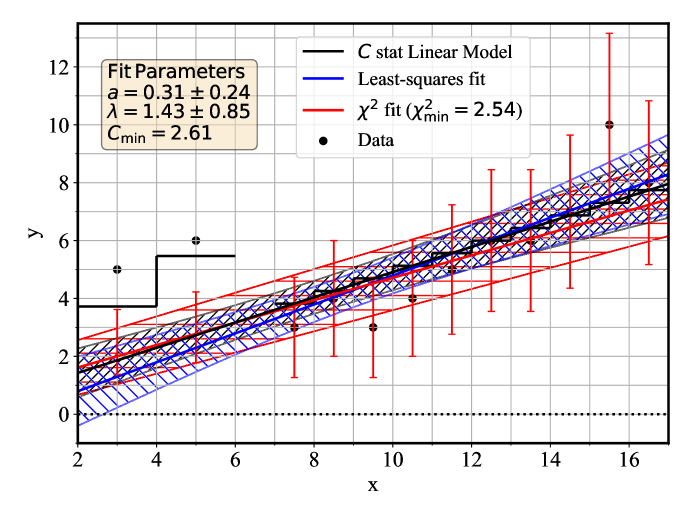
Figure 3: Linear regressions to days 2–17 of the COVID-19 data of Table 1, with a gap in the data, and non–uniform binning. The black curves correspond to the linear regression with the Poisson–based ${C}$ statistic, the blue curves for the ordinary least–squares regression, and the red curves to the $\chi^{2}$ regression that assumes heteroskedastic errors reported as red error bars.

4.3 Fit to days 2–16 with a gap in the data, and non–uniform binning

In this example, the data for days 0 and 1 were ignored, the data for days 2–3 and 4–5 were combined into bins of size $\Delta x=2$ days, the data for day 6 (where no events were reported) were ignored, and the datapoints for days 7–16 were kept with the original binning of $\Delta x=1$ days, for a total of $N=12$ measurements. These choices were simply made for illustration purposes. Specifically, it is generally not advisable to ignore a bin where no counts were recorded, since the non–detection is actually positive information; a case with no counts–in–bin was provided in the previous example. Moreover, the linear regression — and any non–linear regression as well — is sensitive to the choice of bin size. The choice of bin sizes must be dictated by an understanding of the data at hand, and of the scientific goals of the regression.

4.3.1 Poisson regression

The results of the fit to these data are shown in Fig. 3, for best–fit values of $\hat{a}=0.31\pm 0.24$, $\lambda=1.43\pm 0.85$, and an error matrix of

$$\hat{\varepsilon}=\begin{bmatrix}0.716&-0.202\\ -0.202&0.060\end{bmatrix}.$$

It is illustrative to compare this estimate to the one from the error propagation method described in Sect. 3.4, which yields an estimated error matrix of

$$\hat{\varepsilon}_{ep}=\begin{bmatrix}0.687&-0.200\\ -0.200&0.061\end{bmatrix},$$

where the variance of the measurements $y_{k}$ were approximated with the estimated parent means $\hat{\mu}_{k}$. This covariance matrix is nearly identical to the one based on the information matrix, and the small differences between $\hat{\varepsilon}$ and $\hat{\varepsilon}_{ep}$ provide an example of the agreement between the two estimates. Fig. 3 also shows the confidence band for the Poisson regression as the gray hatched area.

4.3.2 Comparison with OLS and $\chi^{2}$ regression

For comparison, a maximum–likelihood regression using the $\chi^{2}$ statistic was also performed for this example, and the results are shown as the red line and confidence band. The ordinary least–squares regression is also shown in blue. For the method of regression that minimizes the $\chi^{2}$ statistic, the data are assumed to be normally–distributed, with variances equal to the number of counts in each bin. Given the variable bin size, the continuous lines therefore represent a density, i.e., the number of counts per unit interval of the $x$ variable, which in this case it is time in units of days. This is reflected in the relationship between the function (1) in units of counts per unit $y$, and the parent mean in (2) in units of pure counts, which are related by the bin size $\Delta x_{i}$. Accordingly, in the $\chi^{2}$ fit with non–uniform binning, the fit statistic is

$$\chi^{2}=\sum_{i=1}^{N}\left(\dfrac{y_{i}-\mu_{i}}{\hat{\sigma}_{i}}\right)^{2}$$

where $\mu_{i}$ is given by (2) with a bin size $\Delta x_{i}=2$ for $i=1,2$, and $\Delta x_{i}=1$ for the other bins. Equivalently, the $\chi^{2}$ regression can be performed directly to the function (1) (or to the linear model with the standard parameterization $a+b\,x$) by re–scaling both the measurements $y_{i}$ and the errors $\hat{\sigma}_{i}$ to counts per unit $y$, since this is the usual assumption in standard software that is used for maximum–likelihood regression for normal data.  Following this method, the first two data points have a count rate of one half the values reported by the black dots, and the $\pm\hat{\sigma}$ error bars for the $\chi^{2}$ regression are illustrated as red vertical lines; those error bars have no meaning for the ${C}$ statistic or the OLS regressions.

The overall slope of the ${C}$ statistic regression line is $a\lambda=0.44\pm 0.11$, while for the $\chi^{2}$ regression it is $0.39\pm 0.13$, and for the least–squares fit it is $0.50\pm 0.08$. The differences, albeit relatively small in this application, are the result of the different assumptions used in the modelling of the data, namely the choice of Poisson versus normal distribution for the number of counts in each bin.

5 Discussion and conclusions

This paper has reviewed the Bonamente and Spence (2022) maximum–likelihood method of linear regression for Poisson count data, and has presented an analytical method for the calculation of the covariance matrix for the parameters of a linear model. For this method of regression, it is found that the parameterization of the model of Equation 1, proposed by Scargle et al. (2013), is quite convenient due to its factorization of the two parameters, which results in convenient algebraic properties for the logarithm of the Poisson likelihood.

The method to obtain the covariance matrix is based on the Fisher information matrix, whose inverse approximates the covariance matrix in the asymptotic limit of a large number of measurement. The key result of this paper is that it is possible to obtain a simple analytical expression for the covariance matrix (Equation 15) that can be used for the Poisson linear regression. This new result, together with the maximum–likelihood estimates of the parameters presented in Bonamente and Spence (2022), offers a simple and accurate method to perform the linear regression on a variety of Poisson–distributed count data, including data with non–uniform binning and with the presence of gaps in the coverage of the independent variable. This method of regression for Poisson–distributed count data is therefore available for use in a variety of data applications, such as the one in the biomedical field presented in Sect. 4.

The paper has also shown that an alternative method for the estimation of the covariance metrix, based on the error propagation or delta method, also provides a simple analytical estimate that is in general good agreement with the method based on the information matrix. The main limitation in the use of the covariance matrix estimated from the information matrix (as well as that from the error propagation method) is that it applies only in the limit of a large number of measurements, where the maximum–likelihood estimates of the parameters are normally–distributed (e.g., Fisher, 1922; Cramer, 1946). In this limit, the variance of the parameters and the covariance can be used for hypothesis testing assuming normal distribution of the parameters.

The maximum–likelihood linear regression to Poisson–distributed count data, presented in this paper and in Bonamente and Spence (2022), have the advantages of being unbiased and asymptotically efficient, in the sense that, in the asymptotic limit of a large number of measurements, the estimators of the linear model parameters have the minimum variance bound according to the Cramér–Rao theorem (Rao 1945, Cramer 1946, see also Rao 1973 and Kendall and Stuart 1973). Given that maximum–likelihood estimators are also known to be consistent in general (see, e.g., Chapter 18 of Kendall and Stuart 1973), this method of regression has very desirable properties for the estimation of the linear model parameters. On the other hand, the ordinary least–squares regression does retain the convenient property of unbiasedness, even for the type of heteroskedastic variances that apply to these Poisson–distributed data. The OLS, however, is not guaranteed to be efficient, in the sense that the variances are in general larger than those of the maximum–likelihood method, and they can also be biased (e.g. Kendall and Stuart, 1973; Swindel, 1968). As a result, the OLS should be viewed as a less accurate method for the regression of Poisson–distributed count data.

Two other methods of linear regression also discussed in this paper, the weighted least–squares and the $\chi^{2}$ methods, suffer from more fundamental shortcomings when applied to integer–count Poisson data. In both cases, it is necessary to know a priori the unequal variances of the data, in order to proceed with the estimation, and this information is simply not available. In particular, the $\chi^{2}$ method is often applied by making the assumption that the variances are equal to the square root of the counts, de facto assuming that the data are normally distributed and with variances equal to the measured counts. Although the Poisson distribution does converge to a normal distribution in the limit of a large number of counts (e.g., see Sect. 3 of Bonamente 2022), the fact that the variance is approximated with the measured counts leads to a bias that remains even in the case of large–count data (e.g. Kelly, 2007; Bonamente, 2020). It is therefore not appropriate to use either of these two methods for the regression of Poisson–distributed count data.

References

- Ahoranta et al. (2020) {barticle}[author] \bauthor\bsnmAhoranta, \bfnmJussi\binitsJ., \bauthor\bsnmNevalainen, \bfnmJukka\binitsJ., \bauthor\bsnmWijers, \bfnmNastasha\binitsN., \bauthor\bsnmFinoguenov, \bfnmAlexis\binitsA., \bauthor\bsnmBonamente, \bfnmMassimiliano\binitsM., \bauthor\bsnmTempel, \bfnmElmo\binitsE., \bauthor\bsnmTilton, \bfnmEvan\binitsE., \bauthor\bsnmSchaye, \bfnmJoop\binitsJ., \bauthor\bsnmKaastra, \bfnmJelle\binitsJ. and \bauthor\bsnmGozaliasl, \bfnmGhassem\binitsG. (\byear2020). \btitleHot WHIM counterparts of FUV O VI absorbers: Evidence in the line-of-sight towards quasar 3C 273. \bjournalA&A \bvolume634 \bpagesA106. \bdoi10.1051/0004-6361/201935846 \endbibitem
- Akaike (1974) {barticle}[author] \bauthor\bsnmAkaike, \bfnmH.\binitsH. (\byear1974). \btitleA new look at the statistical model identification. \bjournalIEEE Transactions on Automatic Control \bvolume19 \bpages716-723. \bdoi10.1109/TAC.1974.1100705 \endbibitem
- Amemiya (1985) {bbook}[author] \bauthor\bsnmAmemiya, \bfnmT.\binitsT. (\byear1985). \btitleAdvanced Econometrics. \bpublisherHarvard University Press. \endbibitem
- Bevington and Robinson (2003) {bbook}[author] \bauthor\bsnmBevington, \bfnmP. R.\binitsP. R. and \bauthor\bsnmRobinson, \bfnmD. K.\binitsD. K. (\byear2003). \btitleData reduction and error analysis for the physical sciences. \bpublisherMcGraw Hill, Third Edition. \endbibitem
- Bonamente (2020) {barticle}[author] \bauthor\bsnmBonamente, \bfnmMassimiliano\binitsM. (\byear2020). \btitleDistribution of the C statistic with applications to the sample mean of Poisson data. \bjournalJournal of Applied Statistics \bvolume47 \bpages2044-2065. \bdoi10.1080/02664763.2019.1704703 \endbibitem
- Bonamente (2022) {bbook}[author] \bauthor\bsnmBonamente, \bfnmM.\binitsM. (\byear2022). \btitleStatistics and Analysis of Scientific Data. \bpublisherSpringer, Graduate Texts in Physics, Third Edition. \endbibitem
- Bonamente and Spence (2022) {barticle}[author] \bauthor\bsnmBonamente, \bfnmMassimiliano\binitsM. and \bauthor\bsnmSpence, \bfnmDavid\binitsD. (\byear2022). \btitleA semi–analytical solution to the maximum–likelihood fit of Poisson data to a linear model using the Cash statistic. \bjournalJournal of Applied Statistics \bvolume49 \bpages522-552. \bdoihttps://doi.org/10.1080/02664763.2020.1820960 \endbibitem
- Cameron and Trivedi (1986) {barticle}[author] \bauthor\bsnmCameron, \bfnmA. Colin\binitsA. C. and \bauthor\bsnmTrivedi, \bfnmPravin K.\binitsP. K. (\byear1986). \btitleEconometric models based on count data. Comparisons and applications of some estimators and tests. \bjournalJournal of Applied Econometrics \bvolume1 \bpages29-53. \bdoihttps://doi.org/10.1002/jae.3950010104 \endbibitem
- Cameron and Trivedi (2013) {bbook}[author] \bauthor\bsnmCameron, \bfnmC.\binitsC. and \bauthor\bsnmTrivedi, \bfnmP. K.\binitsP. K. (\byear2013). \btitleRegression Analysis of Count Data (Second Ed.). \bpublisherCambridge University Press. \endbibitem
- Campbell (1985) {barticle}[author] \bauthor\bsnmCampbell, \bfnmJames E.\binitsJ. E. (\byear1985). \btitleExplaining Presidential Losses in Midterm Congressional Elections. \bjournalThe Journal of Politics \bvolume47 \bpages1140–1157. \endbibitem
- Cash (1979) {barticle}[author] \bauthor\bsnmCash, \bfnmW.\binitsW. (\byear1979). \btitleParameter estimation in astronomy through application of the likelihood ratio. \bjournalAstrophys. J. \bvolume228 \bpages939. \endbibitem
- Clarke (1946) {barticle}[author] \bauthor\bsnmClarke, \bfnmR. D.\binitsR. D. (\byear1946). \btitleAn application of the Poisson distribution. \bjournalJournal of the Institute of Actuaries \bvolume72 \bpages481–481. \bdoi10.1017/S0020268100035435 \endbibitem
- Cramer (1946) {bbook}[author] \bauthor\bsnmCramer, \bfnmH.\binitsH. (\byear1946). \btitleMathematical Methods of Statistics. \bpublisherPrinceton University Press, Princeton. \endbibitem
- Eadie et al. (1971) {bbook}[author] \bauthor\bsnmEadie, \bfnmW. T.\binitsW. T., \bauthor\bsnmDrijiard, \bfnmD.\binitsD., \bauthor\bsnmJames, \bfnmM\binitsM., \bauthor\bsnmRoos, \bfnmM.\binitsM. and \bauthor\bsnmSadoulet, \bfnmB.\binitsB. (\byear1971). \btitleStatistical Methods in Experimental Physics. \bpublisherNorth Holland. \endbibitem
- Fisher (1922) {barticle}[author] \bauthor\bsnmFisher, \bfnmR. A.\binitsR. A. (\byear1922). \btitleOn the mathematical foundations of theoretical statistics. \bjournalPhilosophical Transactions of the Royal Society of London. Series A \bvolume222 \bpages309–368. \endbibitem
- Fisher (1925) {bbook}[author] \bauthor\bsnmFisher, \bfnmR. A.\binitsR. A. (\byear1925). \btitleStatistical Methods for Research Workers. \bpublisherOliver and Boyd, Edinburgh. \endbibitem
- Greenwood and Nikulin (1996) {bbook}[author] \bauthor\bsnmGreenwood, \bfnmP.\binitsP. and \bauthor\bsnmNikulin, \bfnmM.\binitsM. (\byear1996). \btitleA Guide to Chi-Squared Testing. \bpublisherWiley. \endbibitem
- Hilbe (2014) {bbook}[author] \bauthor\bsnmHilbe, \bfnmJoseph M.\binitsJ. M. (\byear2014). \btitleModeling Count Data. \bpublisherCambridge University Press. \bdoi10.1017/CBO9781139236065 \endbibitem
- Kelly (2007) {barticle}[author] \bauthor\bsnmKelly, \bfnmBrandon C.\binitsB. C. (\byear2007). \btitleSome aspects of measurement error in linear regression of astronomical data. \bjournalAstrophys. J. \bvolume665 \bpages1489-1506. \bdoi10.1086/519947 \endbibitem
- Kendall and Stuart (1973) {bbook}[author] \bauthor\bsnmKendall, \bfnmM.\binitsM. and \bauthor\bsnmStuart, \bfnmA.\binitsA. (\byear1973). \btitleThe Advanced Theory of Statistics. Vol.2: Inference and Relationship. \bpublisherHafner, New York 1973, 3rd ed. \endbibitem
- King (1988) {barticle}[author] \bauthor\bsnmKing, \bfnmGary\binitsG. (\byear1988). \btitleStatistical Models for Political Science Event Counts: Bias in Conventional Procedures and Evidence for the Exponential Poisson Regression Model. \bjournalAmerican Journal of Political Science \bvolume32 \bpages838–863. \endbibitem
- Kullback and Leibler (1951) {barticle}[author] \bauthor\bsnmKullback, \bfnmS.\binitsS. and \bauthor\bsnmLeibler, \bfnmR. A.\binitsR. A. (\byear1951). \btitleOn Information and Sufficiency. \bjournalThe Annals of Mathematical Statistics \bvolume22 \bpages79 – 86. \bdoi10.1214/aoms/1177729694 \endbibitem
- Lampton, Margon and Bowyer (1976) {barticle}[author] \bauthor\bsnmLampton, \bfnmM.\binitsM., \bauthor\bsnmMargon, \bfnmB.\binitsB. and \bauthor\bsnmBowyer, \bfnmS.\binitsS. (\byear1976). \btitleParameter estimation in X-ray astronomy. \bjournalAstrophys. J. \bvolume208 \bpages177-190. \bdoi10.1086/154592 \endbibitem
- Levine et al. (1996) {barticle}[author] \bauthor\bsnmLevine, \bfnmAlan M.\binitsA. M., \bauthor\bsnmBradt, \bfnmHale\binitsH., \bauthor\bsnmCui, \bfnmWei\binitsW., \bauthor\bsnmJernigan, \bfnmJ. G.\binitsJ. G., \bauthor\bsnmMorgan, \bfnmEdward H.\binitsE. H., \bauthor\bsnmRemillard, \bfnmRonald\binitsR., \bauthor\bsnmShirey, \bfnmRobert E.\binitsR. E. and \bauthor\bsnmSmith, \bfnmDonald A.\binitsD. A. (\byear1996). \btitleFirst Results from the All-Sky Monitor on the Rossi X-Ray Timing Explorer. \bjournalApJ \bvolume469 \bpagesL33. \bdoi10.1086/310260 \endbibitem
- Lewis and Burke (1949) {barticle}[author] \bauthor\bsnmLewis, \bfnmD.\binitsD. and \bauthor\bsnmBurke, \bfnmC. J\binitsC. J. (\byear1949). \btitleThe use and misuse of the chi-square test. \bjournalPsychological bulletin \bvolume46(6) \bpages433-489. \bdoihttps://doi.org/10.1037/h0059088 \endbibitem
- Luria and Delbrück (1943) {barticle}[author] \bauthor\bsnmLuria, \bfnmS. E.\binitsS. E. and \bauthor\bsnmDelbrück, \bfnmM.\binitsM. (\byear1943). \btitleMutations of bacteria from virus sensitivity to virus resistance. \bjournalGenetics \bvolume28 \bpages491–511. \endbibitem
- McCullagh and Nelder (1989) {bbook}[author] \bauthor\bsnmMcCullagh, \bfnmP.\binitsP. and \bauthor\bsnmNelder, \bfnmJ. A.\binitsJ. A. (\byear1989). \btitleGeneralized Linear Models. \bpublisherChapman & Hall/CRC, Second Edition. \endbibitem
- Poisson (1837) {bbook}[author] \bauthor\bsnmPoisson, \bfnmS. D.\binitsS. D. (\byear1837). \btitleRecherches sur la probabilité des jugements en matière criminelle et en matière civile. \bpublisherParis. \endbibitem
- Rao (1945) {barticle}[author] \bauthor\bsnmRao, \bfnmC. R.\binitsC. R. (\byear1945). \btitleInformation and accuracy attainable in the estimation of statistical parameters. \bjournalBull. Calcutta Math. Soc. \bvolume37 \bpages81. \endbibitem
- Rao (1973) {bbook}[author] \bauthor\bsnmRao, \bfnmC. R.\binitsC. R. (\byear1973). \btitleLinear Statistical Inference and Its Applications. \bpublisherJohn Wiley and Sons, Second Ed. \endbibitem
- Ross (2003) {bbook}[author] \bauthor\bsnmRoss, \bfnmS. M.\binitsS. M. (\byear2003). \btitleIntroduction to Probability Models. \bpublisherAcademic, San Diego. \endbibitem
- Rutherford, Chadwick and Ellis (1920) {bbook}[author] \bauthor\bsnmRutherford, \bfnmE.\binitsE., \bauthor\bsnmChadwick, \bfnmJ.\binitsJ. and \bauthor\bsnmEllis, \bfnmC.\binitsC. (\byear1920). \btitleRadiations from radioactive substances. \bpublisherCambridge University Press. \endbibitem
- Scargle et al. (2013) {barticle}[author] \bauthor\bsnmScargle, \bfnmJeffrey D.\binitsJ. D., \bauthor\bsnmNorris, \bfnmJay P.\binitsJ. P., \bauthor\bsnmJackson, \bfnmBrad\binitsB. and \bauthor\bsnmChiang, \bfnmJames\binitsJ. (\byear2013). \btitleStudies in Astronomical Time Series Analysis. VI. Bayesian Block Representations. \bjournalAstrophys. J. \bvolume764 \bpages167. \bdoi10.1088/0004-637X/764/2/167 \endbibitem
- Shannon and Weaver (1949) {bbook}[author] \bauthor\bsnmShannon, \bfnmClaude E.\binitsC. E. and \bauthor\bsnmWeaver, \bfnmWarren\binitsW. (\byear1949). \btitleThe Mathematical Theory of Communication. \bpublisherUniversity of Illinois Press, \baddressUrbana, IL. \endbibitem
- Swindel (1968) {barticle}[author] \bauthor\bsnmSwindel, \bfnmB. F.\binitsB. F. (\byear1968). \btitleOn the bias of some least-squares estimators of variance in a general linear model. \bjournalBiometrika \bvolume55 \bpages313-316. \bdoi10.1093/biomet/55.2.313 \endbibitem
- New York Times (2021) {bmisc}[author] \bauthor\bsnmNew York Times (\byear2021). \btitleGitHub. \endbibitem
- Wald (1943) {barticle}[author] \bauthor\bsnmWald, \bfnmAbraham\binitsA. (\byear1943). \btitleTests of Statistical Hypotheses Concerning Several Parameters When the Number of Observations is Large. \bjournalTransactions of the American Mathematical Society \bvolume54 \bpages426–482. \endbibitem