Receptivity of compressible boundary layers
over porous surfaces

Abstract

Supersonic pre-transitional boundary layers flowing over porous flat and concave surfaces are studied using numerical and asymptotic methods. The porous wall is composed of thin equally-spaced cylindrical microcavities. The flow is perturbed by small-amplitude, free-stream vortical disturbances of the convected gust type. From the proximity of the leading edge, these external agents generate the compressible Klebanoff modes, i.e. low-frequency disturbances of the kinematic and thermal kind that grow algebraically downstream. For Klebanoff modes with a spanwise wavelength comparable with the boundary-layer thickness, the porous surface has a negligible effect on their growth. When the spanwise wavelength is instead larger than the boundary-layer thickness, these disturbances are effectively attenuated by the porous surface. For a specified set of frequency and wavelengths, the Klebanoff modes evolve into oblique Tollmien-Schlichting waves through a leading-edge-adjustment receptivity mechanism. The wavenumber of these waves is only slightly modified over the porous surface, while the growth rate increases, thus confirming previous experimental results. An asymptotic analysis based on the triple-deck theory confirms these numerical findings. When the wall is concave, the amplitude of the Klebanoff modes is enhanced by the wall curvature and is attenuated by the wall porosity during the initial development.

Accepted for publication in Physical Review Fluids

1 Introduction

Passive control methods aiming to delay laminar-to-turbulent transition in high speed wall flows have been the subject of several studies of numerical, experimental and theoretical nature. The development of new flow control strategies is critical to several aerospace applications ranging from the heat-transfer management on the surface of atmospheric reentry vehicles and in supersonic transport systems (Martin et al., 2012; Schmisseur, 2015) to the design of hypersonic quiet tunnels where the level of noise contamination has to be reduced to a minimum (Schneider, 2008).

Although the inviscid second mode of instability is predominant in high-Mach number boundary layer flows (Mack, 1984), the presence of both the relatively low-frequency first-mode stability disturbances and the laminar streaks triggered by free-stream vorticity has been documented in wind-tunnel experiments. Muñoz et al. (2014) observed streaky structures in the cross flow over a cone in a Ludwieg tube at Mach 6. In the experiments of Hofferth et al. (2013) and Borg et al. (2015), the energy content measured at low frequency was comparable with the energy peak associated with the second instability mode at higher frequency for all the unit Reynolds numbers considered. Graziosi and Brown (2002) also measured large low-frequency disturbances in a pre-transitional Mach-3 boundary layer exposed to vortical and acoustic free-stream fluctuations.

The second mode of instability is effectively attenuated by passive porous coatings. Fedorov and co-workers first showed, in their linear stability and experimental analyses (Malmuth et al., 1998; Fedorov et al., 2001; Rasheed et al., 2002; Fomin et al., 2002; Maslov, 2003), how the presence of a porous surface could result in an attenuation of the acoustic disturbances that propagate within the boundary layer at the expense of a slight enhancement of the Tollmien-Schlichting waves.

This type of porous coatings has the advantage of interacting with small-amplitude disturbances without affecting the laminar base flow. These early analyses paved the way to further studies on ultrasonically absorptive coatings (Fedorov et al., 2006; Wartemann et al., 2012, 2014) and have been extended to include non-regular geometries, acoustic scattering effects, and coupling mechanisms between adjacent pores (Zhao et al., 2018, 2020; Gui et al., 2022). Other researchers have studied surfaces with two-dimensional, equally-spaced grooves of constant width (Brès et al., 2013) and porous surfaces with non-regular microstructures (Sousa et al., 2019). Egorov et al. (2008) investigated the effect of a porous layer on the receptivity of a boundary layer to free-stream disturbances of the acoustic type. In his review paper, Fedorov (2011) advocated further study on porous coatings for the control of boundary-layer receptivity and transient growth.

In the words of Morkovin (1969), the term receptivity refers to the process of internalization of the free-stream disturbances in the boundary layer, their subsequent downstream evolution and the excitation of unstable disturbances. When the disturbance amplitude is relatively high, the early stage of transition in flat-plate boundary layers is dominated by the algebraic growth of externally forced perturbations rather than the exponential amplification of normal modes. The streamwise-elongated fluid structures of nearly constant spanwise wavelength, often referred to as streaks or Klebanoff modes (Kendall, 1985, 1990), reach a saturation level and break down to turbulence through a secondary-instability mechanism (Ricco et al., 2011). Their evolution was the subject of experiments performed in incompressible boundary layers (Westin et al., 1994; Matsubara and Alfredsson, 2001; Fransson et al., 2005). A mathematical description of the incompressible Klebanoff modes was developed by Goldstein and co-workers (Leib et al., 1999) (hereafter referred to as LWG99). Through an asymptotic approach, they unraveled the physical interaction between the disturbances in the free stream and the boundary layer. At downstream locations where the boundary-layer thickness is comparable to the spanwise wavelength of the disturbances, the spanwise diffusion is no longer negligible and the disturbance is described by the unsteady boundary-region equations. The mathematical formulation hinges on the assumption of streamwise-elongated structures, which results in negligible streamwise diffusion and streamwise pressure gradient. The differential problem that arises is of parabolic nature, and thus suitable to a downstream-marching treatment. The computational cost is considerably lower than that required by the numerical solution of the complete Navier-Stokes equations. Goldstein’s theory is based on the precise specification of the initial and boundary conditions and accounts for the effect of the continuous outer forcing on the growth of the Klebanoff modes as the flow evolves downstream. For a review of the theory, the reader is referred to Ricco et al. (2016).

Compressible laminar boundary layers are receptive to free-stream disturbances of the vortical, acoustic, and entropic type (Kovasznay, 1953). The early stages of transition in compressible boundary layers are thus considerably more complex than in the incompressible regime. The rather scarce experimental literature has mainly focused on the role of the acoustic disturbances in supersonic quiet tunnels (Kendall, 1975; Graziosi and Brown, 2002). However, the presence of free-stream vorticity is relevant, as all types of disturbances are present downstream of a shock wave (McKenzie and Westphal, 1968) and exist in supersonic and hypersonic wind tunnels (Schneider, 2008).

The linear incompressible theory of LWG99 was extended to the compressible case (Ricco and Wu, 2007) (RW07), to the nonlinear incompressible case (Ricco et al., 2011) and to the nonlinear compressible case (Marensi et al., 2017). The linear theory well describes the initial growth of the Klebanoff modes, their amplitude still being small and the intermodal coupling negligible. The contribution of each monochromatic mode can be studied separately in this case. The nonlinear theory instead applies when the amplitude of the disturbance flow is comparable with that of the base flow. The combined effect of a continuous free-stream spectrum of vortical disturbances and nonlinearity within the boundary layer was considered by Zhang et al. (2011). Wu and Dong (2016) included the contribution of short-wavelength free-stream disturbances in incompressible and compressible boundary layers. The spanwise and wall-normal wavelengths were comparable with the boundary-layer thickness, that is, they were much shorter than those considered by LWG99.

Free-stream vorticity has also been indicated as a critical cause for the generation and growth of unsteady counter-rotating Görtler vortices (Wu et al., 2011; Viaro and Ricco, 2018, 2019a, 2019b). A laminar boundary layer over a concave wall is subject to an inviscid instability caused by the imbalance between the centrifugal force and the radial pressure gradient. Free-stream vorticity triggers the onset of Klebanoff modes near the leading edge, which, because of the wall curvature, evolve downstream into Görtler vortices, as shown by Wu et al. (2011), Xu et al. (2017) and Xu et al. (2020).

Motivated by Egorov et al. (2008) and Fedorov (2011), we study the effect of porous surfaces on the receptivity of supersonic boundary layers excited by free-stream vortical disturbances and, in particular, on the generation and evolution of compressible Klebanoff modes and highly-oblique Tollmien-Schlichting waves (TS) over these porous surfaces. We adopt the porous-layer model first utilized by Fedorov et al. (2001), which is characterized by a regular microstructure of thin, uniformly-spaced cylindrical pores. To our knowledge, it is the first time that porous surfaces are utilized to control Klebanoff modes over flat and concave porous surfaces. The mathematical framework is discussed in §2. The Klebanoff modes are studied in §3.1 and the receptivity and exponential growth of the TS waves are investigated in §3.2. The combined effect of wall porosity and curvature is the subject of §3.3. Conclusions are presented in §4.

2 Mathematical formulation

A supersonic uniform air flow with free-stream velocity $U_{\infty}^{\ast}$ and static temperature $T_{\infty}^{\ast}$ past an infinitely-thin plate is considered. The flow is described in a Cartesian frame of reference, where $x^{\ast}$, $y^{\ast}$ and $z^{\ast}$ define the streamwise, wall-normal and spanwise coordinates, respectively. The leading edge of the plates is located at $x^{\ast}=y^{\ast}=0$. The Mach number is $\mathrm{M}_{\infty}\equiv U_{\infty}^{\ast}/c_{\infty}^{\ast}$, where $c_{\infty}^{\ast}=\sqrt{\gamma\mathcal{R}^{\ast}T_{\infty}^{\ast}}$ is the speed of sound in the free stream, $\gamma=1.4$ is the heat capacity ratio, and $\mathcal{R}^{\ast}=287.05\,$\mathrm{J}\text{\,}{\mathrm{kg}}^{-1}\text{\,}{\mathrm{K}}^{-1}$$ is the specific gas constant of air. All dimensional quantities are denoted by the superscript ^∗. Schematics of the physical domains are shown in figure 1. Sketch a) depicts the flat-wall system where Klebanoff modes turn into TS waves and sketch b) represents the concave-wall system where Klebanoff modes turn into Görtler vortices. The steady compressible laminar boundary layer forming over the plate is referred to as the base flow (Stewartson, 1964). The free stream is perturbed by small-amplitude, homogeneous disturbances of the convected gust type, i.e. vortical perturbations which are purely advected by the free-stream base flow. The spatial coordinates and all the boundary-layer lengths and wavenumbers are scaled by the spanwise wavelength of the gust, $\lambda_{z}^{\ast}$. The time is scaled by $\lambda_{z}^{\ast}/U_{\infty}^{\ast}$. The velocity components, the density, the viscosity and the temperature are normalized by their free-stream values and the pressure is scaled by $\rho_{\infty}^{\ast}U_{\infty}^{\ast 2}$, where $\rho^{\ast}_{\infty}$ is the density of the fluid in the free stream.

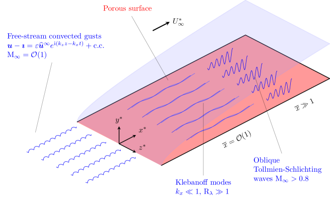
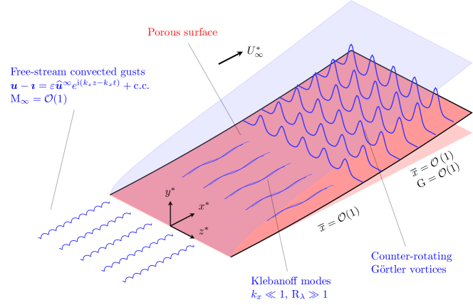
Figure 1: Schematics of the physical domains. Flat-plate system (top) and concave-surface system (bottom).

The focus of the present work is on the early-stage growth of the laminar streaks in a pre-transitional boundary layer. As the amplitude of the perturbations is assumed small, we perform a linear analysis that supports single monochromatic disturbances as the coupling between different modes and secondary instability effects can only be captured in the nonlinear case (Zhang et al., 2011). Albeit idealized, this assumption permits to elucidate important aspects of the receptivity and early-stage growth of the boundary layer streaks (Wu et al., 2011). Moreover, we assume that the perturbations are of low frequency because it is well known that low-frequency, free-stream vortical disturbances are the most likely to generate streamwise-elongated structures in the boundary layer. These structures include the laminar streaks over flat plates (Kendall, 1985, 1990; Westin et al., 1994; Bertolotti, 1997; Fransson et al., 2005), and Görtler vortices on concave surfaces (Wu et al., 2011; Boiko et al., 2017; Viaro and Ricco, 2019a). The spectra of streaks measured by Matsubara and Alfredsson (2001) (figure 9b therein) showed a higher energy content at low frequency and a lower energy content at high frequency compared to the free stream.

The small-amplitude, non-interacting perturbations in the free-stream are modeled by a single monochromatic perturbation of the gust type,

$$\boldsymbol{u}-\boldsymbol{\imath}=\varepsilon\widehat{\boldsymbol{u}}^{\infty}e^{\mathrm{i}\left(k_{z}z-k_{x}t\right)}+\mathrm{c.c.},$$ (1)

where $\boldsymbol{u}$ is the free-stream velocity vector, $\boldsymbol{\imath}$ is the streamwise unit vector, $\varepsilon\ll 1$ indicates the amplitude of the gust, $\widehat{\boldsymbol{u}}^{\infty}=\{\widehat{u}^{\infty},\widehat{v}^{\infty},\widehat{w}^{\infty}\}=\mathcal{O}(1)$, and c.c. its complex conjugate. The gust is characterized by a large wavelength ratio $\lambda_{x}^{\ast}/\lambda_{z}^{\ast}\gg 1$ and a small frequency $k_{x}=\omega^{\ast}\lambda_{z}^{\ast}/U_{\infty}^{\ast}\ll 1$, where $\omega^{\ast}$ is the angular frequency. A Reynolds number $\mathrm{R}_{\lambda}\equiv U_{\infty}^{\ast}\lambda_{z}^{\ast}/\nu_{\infty}^{\ast}\gg 1$ is defined, where $\nu^{\ast}_{\infty}$ is the kinematic viscosity of the fluid in the free stream. We investigate downstream locations at which the base-flow boundary-layer thickness is $\delta=\left(2x/\mathrm{R}_{\lambda}\right)^{1/2}=\mathcal{O}(1)$ and the spanwise and wall-normal diffusions are comparable. A distinguished scaling $k_{x}=\mathcal{O}(R_{\lambda}^{-1})$ emerges (LWG99), as the boundary-layer disturbances evolve downstream on a length scale comparable with the gust streamwise wavelength. The disparity between the spanwise and streamwise scales results in $\mathcal{O}(\varepsilon)$ free-stream fluctuations generating $\mathcal{O}(\varepsilon/k_{x})$ streamwise velocity disturbances within the boundary layer. The mass, momentum, and energy balances of the boundary-layer disturbances are described by the compressible unsteady boundary-region equations (RW07). The small disturbance amplitude relative to that of the base flow allows for their linearization, i.e. for $\varepsilon/k_{x}\ll 1$ or, equivalently, $\varepsilon\mathrm{R}_{\lambda}\ll 1$. Thorough discussions of these scaling relationships are found in LWG99, RW07 and the references therein. The linearization results in a one-way coupling between the base flow and the superposed disturbances. The analysis of the nonlinear effects, which come into play when $\varepsilon\mathrm{R}_{\lambda}=\order{1}$, is beyond the scope of the present study. The influence of nonlinearity on the growth of laminar streaks and Görtler vortices, where the coupling is two-way as the streaks generated within the boundary layer also affect the free-stream disturbances, has been studied by Ricco et al. (2011); Xu et al. (2017); Marensi et al. (2017); Marensi and Ricco (2017) and Xu et al. (2020).

2.1 The laminar base flow

The steady compressible boundary-layer equations are cast into a more compact form by applying the Dorodnitsyn-Howarth coordinate transformation (Stewartson, 1964),

$$\overline{Y}(x,y)\equiv\int_{0}^{y}\rho(x,\breve{y})\ \mathrm{d}\breve{y}.$$ (2)

In the absence of a streamwise pressure gradient, a similarity solution exists and a wall-normal similarity variable

$$\eta\equiv\overline{Y}\left(\frac{\mathrm{R}_{\lambda}}{2x}\right)^{1/2}$$ (3)

is defined. The streamwise velocity, the wall-normal velocity and the temperature of the base flow are

$$\begin{array}[]{ccc}U=F^{\prime}(\eta),&V=(2x\mathrm{R}_{\lambda})^{-1/2}\left(\eta_{c}TF^{\prime}-TF\right),&T=T(\eta),\end{array}$$ (4)

where the prime denotes differentiation with respect to $\eta$ and

$$\eta_{c}\equiv\frac{1}{T}\int_{0}^{\eta}T\left(\breve{\eta}\right)\mathrm{d}\breve{\eta}.$$ (5)

The base-flow solution (4) satisfies the coupled streamwise momentum and energy balance equations

$$\left[\left(\mu/T\right)F^{\prime\prime}\right]^{\prime}+FF^{\prime\prime} =0,$$ (6a)

$$\mathrm{Pr}^{-1}\left[(\mu/T)T^{\prime}\right]^{\prime}+FT^{\prime}+(\gamma-1)\mathrm{M}_{\infty}^{2}(\mu/T)\left(F^{\prime\prime}\right)^{2} =0,$$ (6b)

subject to the boundary conditions

$$\begin{array}[]{ccc}F\left(0\right)=0,&F^{\prime}\left(0\right)=0,&F^{\prime}\left(\infty\right)\to 1\\ T(0)=T_{w},&T\left(\infty\right)\to 1.&\end{array}$$ (7)

The Prandtl number is $\mathrm{Pr}=0.7$. The dynamic viscosity has a power-law dependence on the temperature (Cebeci, 2002),

$$\mu=T^{n}\quad\mbox{with}\quad n=0.76.$$ (8)

This relation is preferred to the Chapman law ($n=1$) as a more accurate model in the supersonic regime (Stewartson, 1964). Appendix A presents a validation study of the computation of the laminar base flow.

2.2 The unsteady disturbance flow

The boundary-layer flow is decomposed as the sum of the base flow and the small-amplitude perturbation flow,

$$\left\{u,\,v,\,w,\,\tau,\,p\right\}=\left\{U,\,V,\,0,\,T,\,-1/2\right\}+\varepsilon\left\{\widetilde{u},\widetilde{v},\widetilde{w},\widetilde{\tau},\widetilde{p}\right\}e^{\mathrm{i}\left(k_{z}z-k_{x}t\right)}+\mathrm{c.c.},$$ (9)

where

$$\left\{\widetilde{u},\widetilde{v},\widetilde{w},\widetilde{\tau},\widetilde{p}\right\}=\left\{\overline{u}_{0},\,\left(\frac{2\overline{x}k_{x}}{\mathrm{R}_{\lambda}}\right)^{1/2}\overline{v}_{0},\,\overline{w}_{0},\,\overline{\tau}_{0},\,\left(\frac{k_{x}}{\mathrm{R}_{\lambda}}\right)^{1/2}\overline{p}_{0}\right\}\left(\overline{x},\eta\right).$$ (10)

The streamwise coordinate is scaled by the gust streamwise wavenumber $k_{x}^{\ast}=2\pi/\lambda_{x}^{\ast}$, i.e. $\overline{x}=k_{x}x=2\pi x^{\ast}/\lambda^{\ast}_{x}=\mathcal{O}(1)$, where $\lambda_{x}^{\ast}$ is the gust streamwise wavelength.

Following Gulyaev et al. (1989); Choudhari (1996) and LWG99, the solution is expanded as a weighted sum of the two-dimensional $\left\{\overline{u}^{(0)},\,\overline{v}^{(0)},\,0,\,\overline{\tau}^{(0)},\,\overline{p}^{(0)}\right\}$ and three-dimensional $\left\{\overline{u},\,\overline{v},\,\overline{w},\,\overline{\tau},\,\overline{p}\right\}$ gust signatures. The evolution of the former was considered by Ricco (2009) for the incompressible case, and is dominant in the outer part of the boundary layer. We focus on the three-dimensional velocity components because they dominate over the two-dimensional components as they exhibit the disturbance growth in the core of the boundary layer. Expanding the solution in terms of the three-dimensional gust signatures yields

$$\left\{\overline{u}_{0},\,\overline{v}_{0},\,\overline{w}_{0},\,\overline{\tau}_{0},\,\overline{p}_{0}\right\}=\left(\widehat{w}^{\infty}+\frac{\mathrm{i}k_{z}\widehat{v}^{\infty}}{\gamma}\right)\left\{\frac{\mathrm{i}k_{z}}{k_{x}}\overline{u},\,\mathrm{i}k_{z}\sqrt{\frac{2\overline{x}}{k_{x}\mathrm{R}_{\lambda}}}\overline{v},\,\overline{w},\,\frac{\mathrm{i}k_{z}}{k_{x}}\overline{\tau},\,\mathrm{i}\kappa_{z}\sqrt{\frac{k_{x}}{\mathrm{R}_{\lambda}}}\overline{p}\right\},$$ (11)

where $\gamma=\left(k_{x}^{2}+k_{z}^{2}\right)^{1/2}$. Their evolution is governed by the compressible linearized unsteady boundary-region (CLUBR) equations (RW07).

The CLUBR equations describe the evolution of the disturbances in the region III of RW07, which occupies locations where $\eta=\mathcal{O}(1)$ and $\overline{x}=\mathcal{O}(1)$ downstream of the leading edge. The CLUBR equations are the limiting form of the compressible Navier-Stokes equations where the streamwise diffusion and the streamwise pressure gradient have been neglected. The boundary-layer thickness is comparable to $\lambda_{z}^{\ast}$ and the contribution of the spanwise diffusion to the momentum and energy balances must be taken into account. The wall-normal and spanwise diffusions are quantified by the asymptotic parameters

$$\kappa_{y} =\frac{k_{y}}{\sqrt{k_{x}\mathrm{R}_{\lambda}}}=\frac{2\pi}{\lambda_{y}^{\ast}}\left(\frac{\nu_{\infty}^{\ast}}{\omega^{\ast}}\right)^{1/2}=\mathcal{O}(1),$$ (12a)

$$\kappa_{z} =\frac{k_{z}}{\sqrt{k_{x}\mathrm{R}_{\lambda}}}=\frac{2\pi}{\lambda_{z}^{\ast}}\left(\frac{\nu_{\infty}^{\ast}}{\omega^{\ast}}\right)^{1/2}=\mathcal{O}(1).$$ (12b)

Free-stream gusts with equivalent wavenumbers $\kappa_{y}=\kappa_{z}$ are considered. The initial and boundary conditions are discussed in §2.2.1 and the modelling of the porous layer is presented in §2.2.2 and §2.2.3. The CLUBR equations are given in Appendix B (Viaro and Ricco, 2019a) and the details of their derivation are found in Ricco (2006).

2.2.1 Boundary and initial conditions

The CLUBR equations are subject to wall and free-stream boundary conditions that synthesize how the boundary layer interacts with the porous wall and the external disturbance flow. Being parabolic along $\overline{x}$, the CLUBR equations also require initial conditions for $\overline{x}\ll 1$.

The no-slip wall boundary condition is applied to the streamwise and spanwise disturbance velocities, i.e. $\overline{u}=\overline{w}=0$ at $\eta=0$. At the wall, the wall-normal velocity and the temperature are related to the pressure because of the wall porosity, as follows

$$\overline{v}\left(\eta=0\right) =\frac{\overline{A}_{v}}{(2\overline{x})^{1/2}}\overline{p}\left(\eta=0\right),$$ (13a)

$$\overline{\tau}\left(\eta=0\right) =\frac{\overline{A}_{\tau}}{(2\overline{x})^{1/2}}\overline{p}\left(\eta=0\right),$$ (13b)

where $\overline{A}_{v}$ and $\overline{A}_{\tau}$ are the scaled admittances, obtained in §2.2.3. The free-stream boundary conditions are the same as in RW07,

$$\left\{\overline{u},\,\overline{\tau}\right\} \rightarrow 0,$$ (14a)

$$\left(\frac{\partial}{\partial\eta}+\left|{\kappa_{z}}\right|\left(2\overline{x}\right)^{1/2}\right)\left\{\overline{v},\,\overline{w},\,\overline{p}\right\} \rightarrow\left\{-1,\,\mathrm{i}\kappa_{y}(2\overline{x})^{1/2},\,0\right\}e^{\mathrm{i}\left(\overline{x}+\kappa_{y}\left(2\overline{x}\right)^{1/2}\overline{\eta}\right)}e^{-\left(\kappa_{y}^{2}+\kappa_{z}^{2}\right)\overline{x}},$$ (14b)

as $\eta\rightarrow\infty$, where $\overline{\eta}\equiv\eta-\beta_{c}$, and $\beta_{c}=\lim_{\eta\rightarrow\infty}(\eta-F)$. The wall-normal wavenumber $\kappa_{y}$ only appears in (14) and not in the CLUBR equations because the wall-normal length scale of the free-stream flow is $\lambda^{\ast}_{y}$, while, within the boundary layer, the characteristic length scale is the boundary-layer thickness.

The initial conditions are the same as in RW07. As they pertain to a non-porous wall, the wall porosity increases smoothly from zero at small $\overline{x}$ to a finite value downstream according to the function proposed by Negi et al. (2015), as discussed in §2.2.3. A few comments about the initial conditions are in order. The plate is assumed to be infinitely thin and therefore the free-stream base flow is not distorted at leading order as the fluid encounters the flat plate. The only distortion of the base-flow streamlines is produced by the thickening of the boundary layer. As the free-stream disturbances are transported by the base flow, they are neither stretched nor tilted by the leading edge. The leading-edge bluntness effects can play a central role on the free-stream distortion and therefore on the boundary-layer response. This problem is however out of the scope of the present study because these effects only occur when the characteristic dimension of the rounded leading edge is comparable with the spanwise length scale (Goldstein et al., 1992; Goldstein and Leib, 1993; Goldstein and Wundrow, 1998; Goldstein, 2014). Furthermore, the disturbance flow in the very proximity of the leading edge is not considered because the inviscid flow outside of the boundary layer is solved for $x\gg 1$, i.e. at a distance much larger than the spanwise wavelength. As discussed in LWG99, streamwise-decaying disturbances emerging from the interaction between the free-stream vorticity disturbances and the leading edge, obtained by Choudhari (1996) by using the Wiener-Hopf technique, decay to a very small amplitude when $x\gg 1$ and, therefore, they play a negligible role in the boundary-layer response. As the initial conditions are obtained by taking the limit $\overline{x}\ll 1$ of the CLUBR equations, they constitute the asymptotically rigorous upstream behaviour of the CLUBR solution at locations $1\ll x\ll k_{x}^{-1}$ or, in dimensional form, at locations $\lambda_{z}^{*}\ll x^{*}\ll\lambda_{x}^{*}$.

The base-flow solutions (4) are computed using a second-order accurate Keller-box method (Cebeci, 2002). The CLUBR system, given in Appendix B, is solved by a second-order finite-difference scheme that is central in $\eta$ and backward in $\overline{x}$. A standard block-elimination algorithm is utilized (Cebeci, 2002). The free-stream boundary conditions (14) are applied by a second-order finite-difference discretization scheme. The pressure is computed on a grid staggered along the $\eta$ direction with respect to that for the velocity in order to avoid the pressure decoupling phenomenon.

2.2.2 The unsteady disturbance flow within the pores

The flow inside a pore in studied in this section. In the porous wall designed by Fedorov et al. (2001), the pressure fluctuations at the interface between the wall and the boundary layer excite kinematic and thermal disturbances in long, thin cylindrical pores. The numerical studies of Zhao et al. (2018, 2020) showed that the effects of acoustic scattering between adjacent pores can be neglected when the Helmholtz number $\mathrm{He}=\omega^{\ast}H^{\ast}/c_{w}^{\ast}<4.21$, where $H^{\ast}$ is the depth of the pores and $c_{w}^{\ast}=\sqrt{\gamma\mathcal{R}^{\ast}T_{w}^{\ast}}$ the speed of sound in the pores. All the cases considered in the present work comply with that condition. Hence, the properties of the porous layer can be studied by considering the flow characteristics of an isolated pore. The equations that govern the propagation of small-amplitude disturbances in a single dead-end circular pore of depth $H^{\ast}$ and radius $R^{\ast}$ are reported in Appendix C. The linearized continuity, axial momentum and energy equations are cast in cylindrical coordinates, and their solution yields an analytical radial distribution of the velocity and temperature in the form of Bessel functions (Zwikker and Kosten, 1949; Fedorov et al., 2001).

The response of the pores is ruled by the frequency parameter $k_{x}\mathrm{R}_{\lambda}$ (Fedorov et al., 2001; Goldstein and Ricco, 2018; Viaro and Ricco, 2019a). The disturbances are not transmitted to the pores at very low frequencies, for which the frequency parameter $k_{x}\mathrm{R}_{\lambda}=\mathcal{O}\left({1}\right)$ or smaller. The boundary-layer disturbances are expected to interact with the porous wall as $k_{x}\mathrm{R}_{\lambda}$ increases and the magnitude of the spanwise diffusion, proportional to $\kappa_{z}$ in (12), decreases. We are therefore interested in investigating the behaviour of the porous layer for $k_{x}\mathrm{R}_{\lambda}\gg 1$. The terms of the momentum and energy balances in (69) are scaled as in the boundary layer and the parameter

$$K_{v}=R^{\ast}\left(\frac{\rho_{w}^{\ast}\omega^{\ast}}{\mu_{w}^{\ast}}\right)^{1/2}=R\left(\frac{k_{x}\mathrm{R}_{\lambda}}{\mu_{w}T_{w}}\right)^{1/2}\gg 1$$ (15)

is introduced, where $\rho_{w}^{\ast}$ and $\mu_{w}^{\ast}$ are the base-flow density and dynamic viscosity at the wall. The balance equations reveal a boundary-layer structure (Bender and Orszag, 1999) for the velocity and temperature fluctuations, whose values depend on the radial coordinate $r$, while the pressure is only a function of the axial coordinate $y$ and is the same inside and outside the boundary layer. The outer solutions are obtained by imposing $K_{v}^{-1}=0$, for which the full system (69) in Appendix C reduces to the equation for the pressure

$$\frac{\mathrm{d}^{2}\widetilde{p}}{\mathrm{d}y^{2}}+\mathrm{He}^{2}\widetilde{p}=0,$$ (16)

which arises from a reduction of a Helmholtz equation. The outer solutions for the velocity and pressure fluctuations are found,

$$\widetilde{p}=\widetilde{p}_{out}\left(y\right) =a\cos{\left[\mathrm{He}\left(y+1\right)\right]},$$ (17a)

$$\widetilde{v}=\widetilde{v}_{out}\left(y\right) =-\mathrm{i}\frac{\mathrm{d}\widetilde{p}}{\mathrm{d}y}=\mathrm{i}a\sin{\left[\mathrm{He}\left(y+1\right)\right]},$$ (17b)

$$\widetilde{\tau}=k_{x}^{2}\widetilde{\tau}_{out}\left(y\right) =k_{x}^{2}\left(\gamma-1\right)a\frac{\mathrm{M}_{\infty}^{2}H^{2}}{T_{w}}\cos{\left[\mathrm{He}\left(y+1\right)\right]},$$ (17c)

where $a$ is a real constant. The pressure and temperature fluctuations are in phase in the outer region. In the proximity of the wall, i.e. where $r-1\ll 1$, an inner variable

$$r_{s}=K_{v}\left(1-r\right)=\mathcal{O}(1)$$ (18)

describes the inner solutions $\widetilde{v}_{in}\left(r_{s},y\right)$ and $k_{x}^{2}\widetilde{\tau}_{in}\left(r_{s},y\right)$. Upon introduction of the inner variable, the momentum and energy balance equations take the form

$$-\mathrm{i}\widetilde{v}_{in}+\frac{\mathrm{d}\widetilde{p}_{out}}{\mathrm{d}y} =\frac{\partial^{2}\widetilde{v}_{in}}{\partial r_{s}^{2}},$$ (19a)

$$-\mathrm{i}\widetilde{\tau}_{in}+\mathrm{i}\left(\gamma-1\right)\frac{\mathrm{M}_{\infty}^{2}L^{2}}{T_{w}}\widetilde{p}_{out} =\frac{1}{\mathrm{Pr}}\frac{\partial^{2}\widetilde{\tau}_{in}}{\partial r_{s}^{2}},$$ (19b)

subject to the boundary conditions

$$\widetilde{v}_{in}\left(0;y\right)=\widetilde{\tau}_{in}\left(0;y\right) =0,$$ (20a)

$$\lim_{r_{s}\to\infty}\widetilde{v}_{in}\left(r_{s};y\right) =\widetilde{v}_{out}\left(y\right),$$ (20b)

$$\lim_{r_{s}\to\infty}\widetilde{\tau}_{in}\left(r_{s};y\right) =\widetilde{\tau}_{out}\left(y\right).$$ (20c)

The inner solutions are

$$\widetilde{v}_{in}\left(r;y\right) =\widetilde{v}_{out}\left(y\right)\left[1-\exp\left(\mathrm{i}^{3/2}K_{v}\left(r-1\right)\right)\right],$$ (21a)

$$\widetilde{\tau}_{in}\left(r;y\right) =\widetilde{\tau}_{out}\left(y\right)\left[1-\exp\left(\mathrm{i}^{3/2}\mathrm{Pr}^{1/2}K_{v}\left(r-1\right)\right)\right].$$ (21b)

The solutions (21) represent azimuthal Stokes layers of velocity and temperature attached to the pore wall. The cross-sectional averages of the axial velocity (21a) and the temperature perturbations (21b) over the circular section of a pore are

$$\left\langle\widetilde{v}_{in}\right\rangle\left(r;y\right) =\widetilde{v}_{out}\left(y\right)\left[1+2\mathrm{i}\frac{\displaystyle\exp\left(-\mathrm{i}^{3/2}K_{v}\right)+\mathrm{i}^{3/2}K_{v}-1}{K_{v}^{2}}\right],$$ (22a)

$$\left\langle\widetilde{\tau}_{in}\right\rangle\left(r;y\right) =\widetilde{\tau}_{out}\left(y\right)\left[1+2\mathrm{i}\frac{\displaystyle\exp\left(-\mathrm{i}^{3/2}\mathrm{Pr}^{1/2}K_{v}\right)+\mathrm{i}^{3/2}\mathrm{Pr}^{1/2}K_{v}-1}{\mathrm{Pr}K_{v}^{2}}\right].$$ (22b)

Figure 2a shows that the agreement between the Bessel-function solutions, given in (70) of Appendix C, and the asymptotic solution (21a) improves as $K_{v}$ increases, the lines being indistinguishable for $K_{v}=33$. For $K_{v}\gg 1$, the cross-sectional average of the Bessel-function axial velocity (71a) can also be obtained by using the asymptotic expansion for large arguments of the Bessel function. The leading order terms (Abramowitz and Stegun, 1970)

$$J_{m}\left(\xi\right)=\left(\frac{2}{\pi\xi}\right)^{1/2}\cos{\left(\xi-\frac{m\pi}{2}-\frac{\pi}{4}\right)}\mbox{, }m=0,1,2,\dots$$ (23)

yield the relation

$$\left\langle{\widetilde{v}_{in}}\right\rangle\left(y\right)=\widetilde{v}_{out}\left[1-\frac{\cos{\left(\mathrm{i}^{1/2}K_{v}-3\pi/4\right)}}{\mathrm{i}^{1/2}K_{v}\cos{\left(\mathrm{i}^{1/2}K_{v}-\pi/4\right)}}\right].$$ (24)

The real and imaginary parts of (71a), (24), and (21) are normalized with respect to $\widetilde{v}_{out}$ and plotted in figure 2b. The difference between the real parts becomes indiscernible for $K_{v}>4$, whereas the imaginary parts match excellently for $K_{v}>10$. The ratio

$$\frac{\left\langle{\widetilde{v}_{in}}\right\rangle}{\widetilde{v}_{out}}=A_{v}\frac{\widetilde{p}}{\widetilde{v}_{out}}$$ (25)

represents a normalized acoustic admittance, where the normalization factor is the large-$K_{v}$ limit of $A_{v}$.

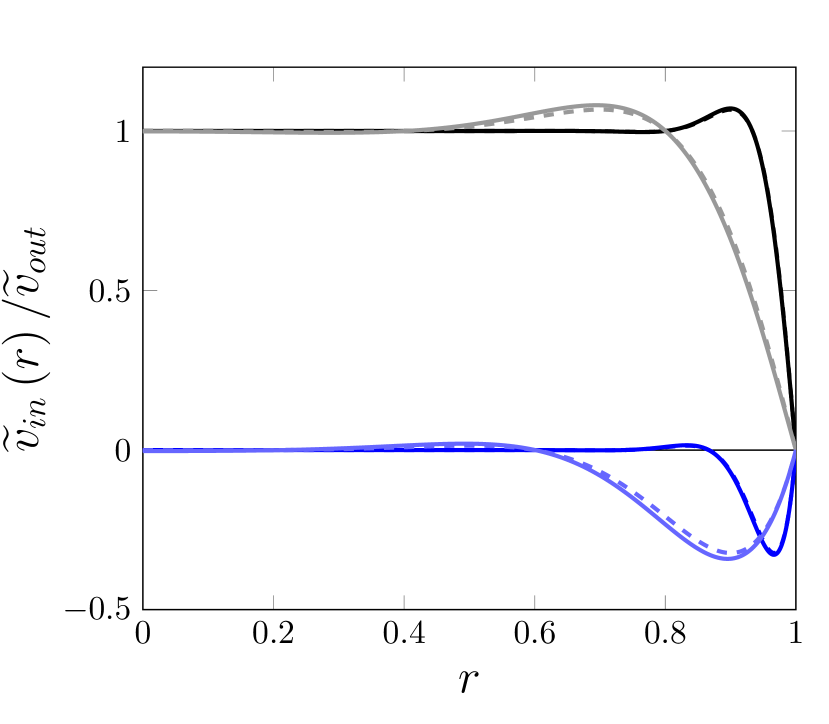
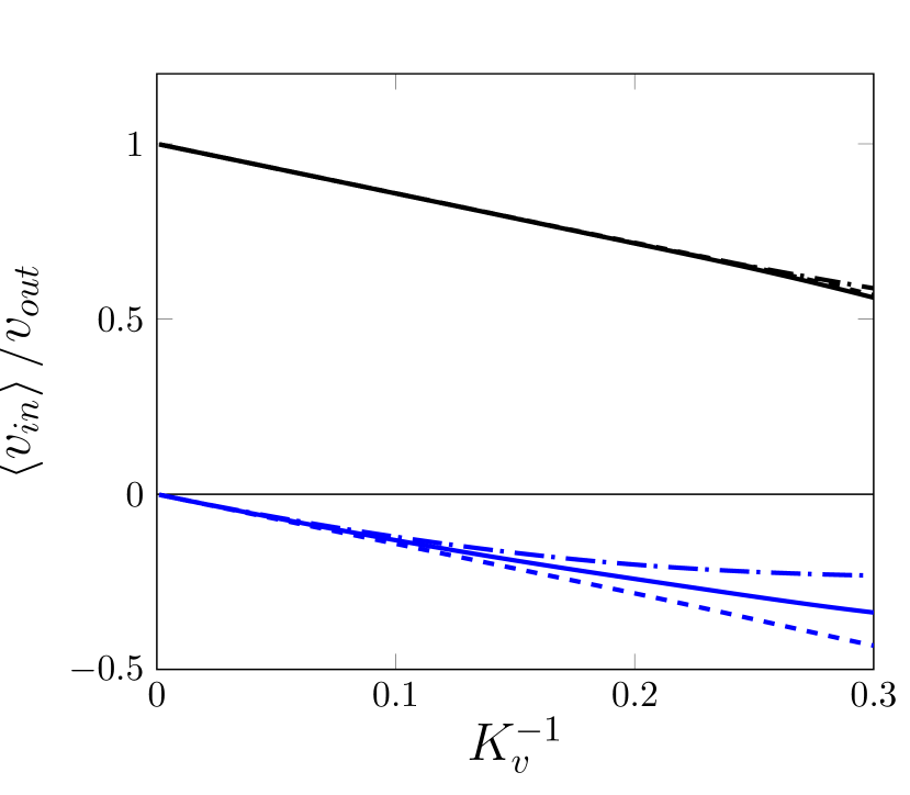
Figure 2: (a) Radial distribution of the axial velocity within a pore at a given depth for $K_{v}=11$ (grey for real part and light blue for imaginary part) and $K_{v}=33$ (black for real part and dark blue for imaginary part). The Bessel-function solutions (70a, solid lines) are compared with the asymptotic solutions (21a, dashed lines). (b) Averaged Bessel-function solutions (70a, solid lines), averaged asymptotic solutions (21a, dashed curves), and averaged Bessel-function solutions obtained with the asymptotic form of the Bessel functions for large arguments (23, dash-dotted lines) for $K_{v}=11$ (blue lines) and $K_{v}=33$ (black lines).

2.2.3 Porous admittance

Following Fedorov et al. (2001), the wall-normal velocity disturbance and the temperature disturbance are related to the pressure disturbance as follows,

$$\widetilde{v}\left(\eta=0\right) =A_{v}\widetilde{p}\left(\eta=0\right),$$ (26a)

$$\widetilde{\tau}\left(\eta=0\right) =A_{\tau}\widetilde{p}\left(\eta=0\right),$$ (26b)

where $A_{v}$ and $A_{\tau}$ are the complex admittances of the porous wall evaluated at the wall-boundary layer interface ($\eta=0$). They are derived in Appendix C. The velocity admittance is

$$A_{v}=-\phi\frac{\mathrm{i}\Lambda}{L}\left[1-\mathcal{F}\left(\mathrm{i}^{1/2}K_{v}\right)\right]\tanh{\Lambda},$$ (27)

where

$$\Lambda=\frac{\mathrm{i}k_{x}\mathrm{M}_{\infty}L}{T_{w}^{1/2}}\mathcal{H}\left(\mathrm{i}^{1/2}K_{v}\right),$$ (28)

$$\mathcal{H}\left(\mathrm{i}^{1/2}K_{v}\right)=\left[\frac{1+\left(\gamma-1\right)\mathcal{F}\left(\left(\mathrm{i}\mathrm{Pr}\right)^{1/2}K_{v}\right)}{1-\mathcal{F}\left(\mathrm{i}^{1/2}K_{v}\right)}\right]^{1/2},$$ (29)

and $\mathcal{F}$ is given by (72). The porosity $\phi$ is defined as the ratio between the surface area of the pores and the total surface area. By combining (27) and (28), the admittance of the velocity is rewritten as

$$A_{v}=\phi\frac{k_{x}\mathrm{M}_{\infty}}{T_{w}^{1/2}}\mathcal{G}\left(\mathrm{i}^{1/2}K_{v}\right)\tanh{\Lambda},$$ (30)

where

$$\mathcal{G}\left(\mathrm{i}^{1/2}K_{v}\right)=\left[\left(1-\mathcal{F}\left(\mathrm{i}^{1/2}K_{v}\right)\right)\left(1+\left(\gamma-1\right)\mathcal{F}\left(\left(\mathrm{i}\mathrm{Pr}\right)^{1/2}K_{v}\right)\right)\right]^{1/2}.$$ (31)

Figures 3a and 3b show the real and imaginary parts of $\mathcal{G}$ and $\mathcal{H}$, respectively.

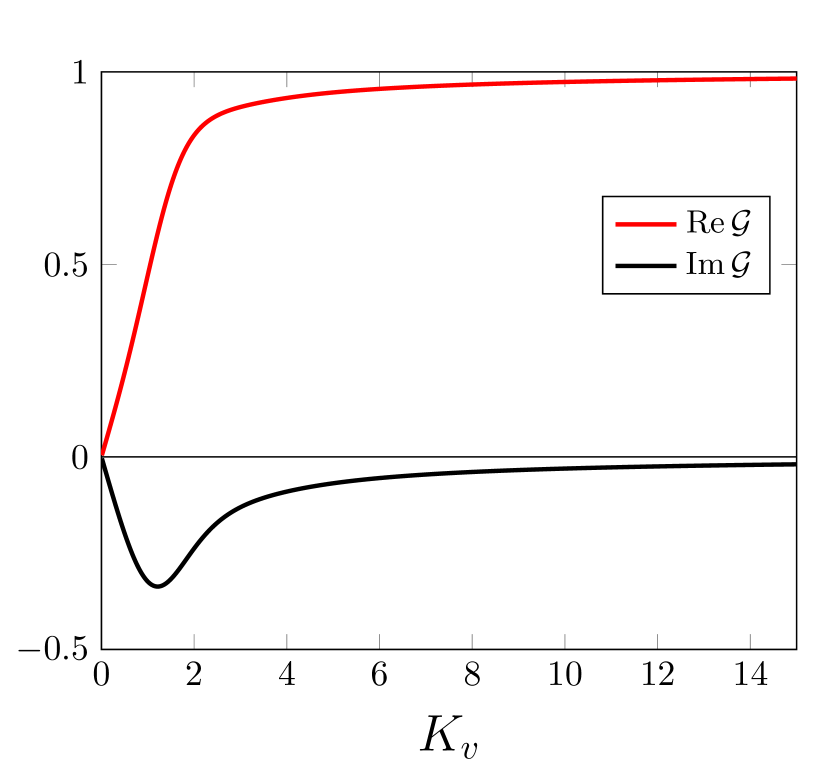
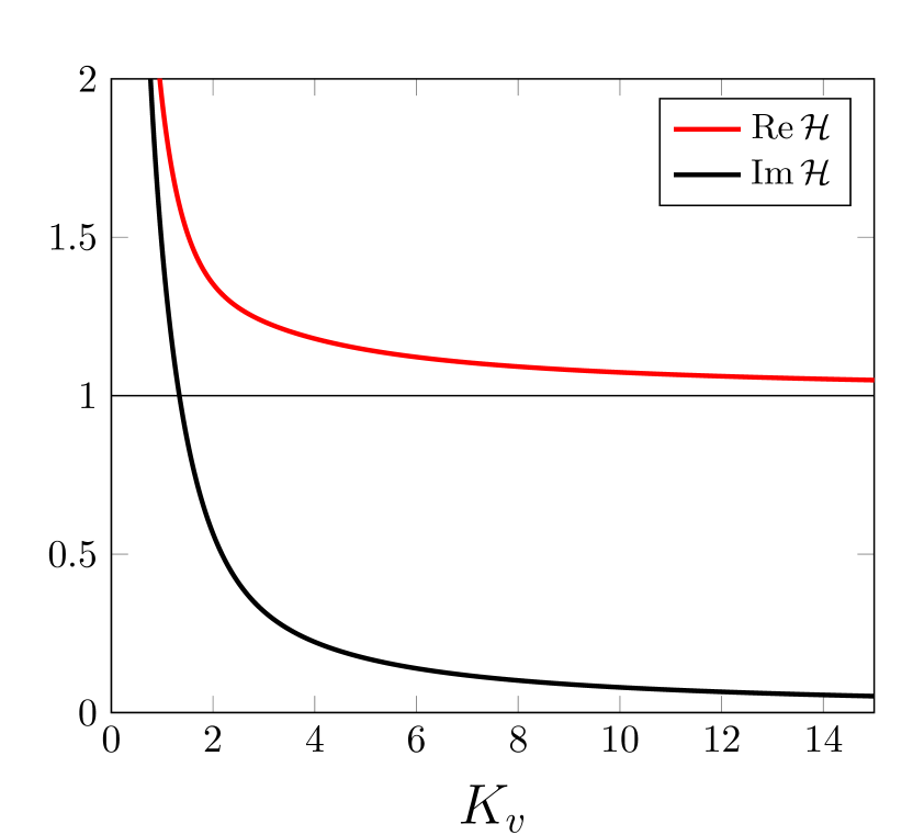
Figure 3: Real and imaginary parts of $\mathcal{G}$ and $\mathcal{H}$ as functions of $K_{v}$, given by the Bessel-function solutions (31) and (29), respectively.

The thermal admittance (77b) reads

$$A_{\tau}=\left(\gamma-1\right)\frac{k_{x}^{2}\mathrm{M}_{\infty}^{2}L^{2}}{T_{w}}\left[1-\mathcal{F}\left(\left(\mathrm{i}\mathrm{Pr}\right)^{1/2}K_{v}\right)\right].$$ (32)

By introducing the expressions of the boundary-layer disturbances (11) and by using (12), one finds

$$\overline{v}\left(\eta=0\right) =\frac{k_{x}\kappa_{z}A_{v}}{(2\overline{x})^{1/2}k_{z}}\overline{p}\left(\eta=0\right)=\left(\frac{k_{x}}{2\overline{x}\mathrm{R}_{\lambda}}\right)^{1/2}A_{v}\overline{p}\left(\eta=0\right),$$ (33a)

$$\overline{\tau}\left(\eta=0\right) =\frac{k_{x}A_{\tau}}{\mathrm{R}_{\lambda}}\overline{p}\left(\eta=0\right).$$ (33b)

The wall boundary conditions (33a) and (33b) are rewritten by using $\overline{A}_{v}=\left(k_{x}\mathrm{R}_{\lambda}^{-1}\right)^{1/2}A_{v}$ and $\overline{A}_{\tau}=\left(k_{x}\mathrm{R}_{\lambda}^{-1}\right)A_{\tau}$ in (13a) and (13b). The velocity admittance $A_{v}$ defined in (30) is $\mathcal{O}\left({k_{x}}\right)$ and the thermal admittance $A_{\tau}$ (32) is $\mathcal{O}\left({k_{x}^{2}}\right)$. The coefficients in front of the pressure in (33a) and (33b) are $\mathcal{O}\left(k_{x}^{3/2}\mathrm{R}_{\lambda}^{-1/2}\right)$ and $\mathcal{O}\left(k_{x}^{3}\mathrm{R}_{\lambda}^{-1}\right)$, respectively. The contribution of $A_{\tau}$ to the temperature fluctuations is thus much weaker than the contribution of $A_{v}$ to the velocity fluctuations and therefore negligible. However, the porous wall affects the temperature fluctuations indirectly because of the coupling between the wall-normal momentum equation and the energy equation. For typical Klebanoff modes and Görtler vortices $k_{x}\mathrm{R}_{\lambda}=\order{1}$, $A_{v}=\order{\mathrm{R}_{\lambda}^{-2}}$, $A_{v}=\order{\mathrm{R}_{\lambda}^{-4}}$, and wall porosity has a negligible effect on both the velocity and temperature fluctuations. As shown in §2.2.2 the pores begin interacting with the disturbance flow when $k_{x}\mathrm{R}_{\lambda}\gg 1$. Since the pressure and temperature fluctuations are in phase within the pores, the adiabatic boundary condition can be imposed at the wall in accordance with the homogeneous Neumann boundary condition at the dead end of the pores, as discussed in Appendix C.

Since the upstream boundary conditions for $\overline{x}\ll 1$ are not compatible with a non-zero wall-normal velocity at $\eta=0$, a short smoothing region along the streamwise direction is introduced between two streamwise coordinates $\overline{x}_{1}$ and $\overline{x}_{2}$ in the vicinity of the leading edge. In this region, the velocity admittance varies proportionally to (Negi et al., 2015)

$$S(\overline{x})=\begin{cases}0,&\text{for \ $\overline{x}\leq\overline{x}_{1}$},\\ \left[1+\exp\left(\displaystyle{\frac{1}{\widetilde{x}-1}+\frac{1}{\widetilde{x}}}\right)\right]^{-1},&\text{for \ $\overline{x}_{1}<\overline{x}<\overline{x}_{2}$},\\ 1,&\text{for $\overline{x}\geq\overline{x}_{2}$},\end{cases}$$ (34)

where $\widetilde{x}=(\overline{x}-\overline{x}_{1})/(\overline{x}_{2}-\overline{x}_{1})$, and $\overline{x}_{1}=0.005$. The end point is $\overline{x}_{2}=0.01$, if exception is made for the analysis at the end of §3.1, where the effect of $\overline{x}_{2}$ is studied. The piecewise function (34) can be physically interpreted as a variation of the wall porosity along the smoothing region. If we assume the pores to be aligned in equally spaced rows and columns, such variation may be caused by pores of constant radius $R^{\ast}$ becoming more and more packed as the distance $d^{\ast}$ between the centres of adjacent pores decreases, or by the gradual increase of the pore radius. In both cases, the porosity in (30) can be written as $\phi=\pi R_{f}^{\ast 2}S(\overline{x})/d_{f}^{\ast 2}$, where the subscript $f$ denotes quantities at the downstream end of the smoothing region. If the radius is kept constant between $\overline{x}_{1}$ and $\overline{x}_{2}$, the interpore distance is $d^{\ast}(\overline{x})=d_{f}^{\ast}/\sqrt{S(\overline{x})}$. The porosity at the end of the smoothing region is thus $\phi=\pi R_{f}^{\ast 2}/d_{f}^{\ast 2}$. As only regularly-spaced circular pores are considered, the porosity may attain a maximum theoretical value of $\pi/4$ when $R_{f}^{\ast}=d_{f}^{\ast}/2$.

3 Results

The effectiveness of the porous wall depends on its ability to transduce a pressure disturbance into a wall-normal velocity disturbance, as described by (33a). In the present coatings, the phase velocity of the disturbances is equivalent to the local sound speed (Brès et al., 2013). For $K_{v}\gg 1$, a dimensional analysis of the boundary condition (33a) and the velocity admittance (30) yields

$$\frac{\overline{v}}{\overline{p}}=\mathcal{O}\left({\left(\frac{k_{x}^{3}}{R_{\lambda}}\right)^{1/2}\frac{\mathrm{M}_{\infty}}{T_{w}^{1/2}}}\right)=\mathcal{O}\left({\frac{\omega^{\ast 3/2}\lambda_{z}^{\ast}}{U_{\infty}^{\ast}c_{w}^{\ast}}\nu_{\infty}^{\ast 1/2}}\right).$$ (35)

As a result, the pores interact with the boundary layer when

$$\omega^{\ast 3/2}\lambda_{z}^{\ast}\mbox{ is comparable with }U_{\infty}^{\ast}c_{w}^{\ast}\nu_{\infty}^{\ast-1/2}.$$ (36)

A visual representation of relation (36) is shown in figure 4. The free-stream velocity, the free-stream kinematic viscosity and the speed of sound in the porous layer define the threshold above which the boundary-layer disturbances are affected by the porous layer. For given free-stream conditions, the effect of the porous layer is more intense at lower $c_{w}^{\ast}$. For a given $\lambda_{z}^{\ast}$ and constant free-stream conditions, the minimum frequency at which a disturbance is affected grows as $T_{w}^{\ast 1/3}$. The minimum wavelength for which a disturbance is attenuated at a given frequency increases as $T_{w}^{\ast 1/2}$. Both hyperbolas shift away from the origin as $c_{w}^{\ast}$ increases. Relation (36) also shows that the variation of the frequency is more influential on the performance of the porous wall than that of the spanwise wavelength.

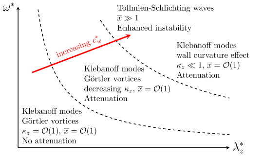
Figure 4: Schematic of flow regimes and the effect of wall porosity, as described by relation (36).

Physical parameter	Symbol	Value	SI unit
Mach number	$\mathrm{M}_{\infty}$	$6$	-
Total (stagnation) temperature	$T_{0}^{\ast}$	400	$\mathrm{K}$
Static pressure	$p_{\infty}^{\ast}$	633	$\mathrm{Pa}$
Static temperature	$T_{\infty}^{\ast}$	49	$\mathrm{K}$
Free-stream velocity	$U_{\infty}^{\ast}$	841	$\mathrm{m}\text{\,}{\mathrm{s}}^{-1}$
Free-stream kinematic viscosity	$\nu_{\infty}^{\ast}$	$6.3\cdot 10^{-5}$	$\mathrm{m}^{2}\mathrm{/}\mathrm{s}$
Unit Reynolds number	$\mathrm{R}^{\ast}=U_{\infty}^{\ast}/\nu_{\infty}^{\ast}$	$13.5\cdot 10^{6}$	${\mathrm{m}}^{-1}$
Recovery temperature	$T^{\ast}_{a,w}$	343	$\mathrm{K}$
Wall temperature	$T_{w}^{\ast}=0.8T^{\ast}_{a,w}$	274	$\mathrm{K}$
Pore radius	$R^{\ast}$	$90$	$\mathrm{\SIUnitSymbolMicro m}$
Inter-pore distance	$d^{\ast}$	$210$	$\mathrm{\SIUnitSymbolMicro m}$
Pore depth	$H^{\ast}$	$1.5$	$\mathrm{mm}$
Porosity	$\phi$	$0.58$	-
Velocity admittance	$\overline{A}_{v}$	$-8.82\cdot 10^{-4}+1.434\cdot 10^{-3}\ \mathrm{i}$	-

Table 1: Physical parameters for wind tunnel conditions.

The physical parameters of the present study are listed in table 1. These values are representative of supersonic quiet tunnel conditions, such as those of the Sandia Hypersonic Wind tunnel and the Boeing Mach 6 quiet tunnel (Casper et al., 2009). The stagnation temperature of $400\,$\mathrm{K}$$ and the wall-temperature ratio of $T_{w}^{\ast}/T_{ad,w}^{\ast}=0.8$ (where $T_{ad,w}^{*}$ is the adiabatic-wall temperature) are given by Shiplyuk et al. (2004); Casper et al. (2009); Schneider (2008) and Yu et al. (2018).

3.1 Klebanoff modes

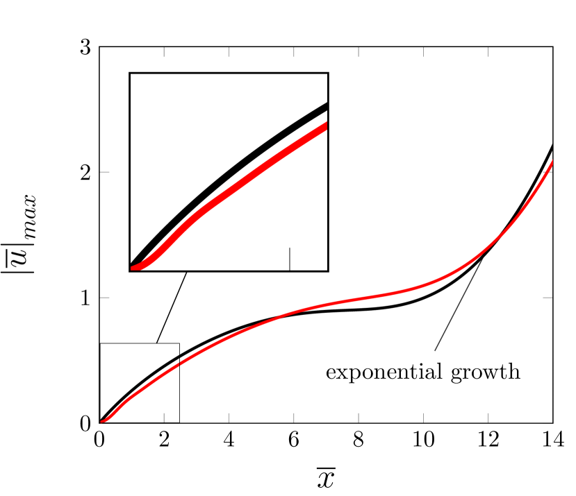
(a) $\kappa_{z}=0.008$, $k_{x}/k_{z}=0.24$.

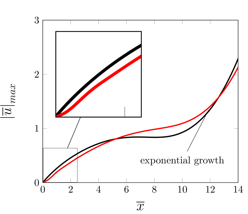
(b) $\kappa_{z}=0.0075$, $k_{x}/k_{z}=0.27$.

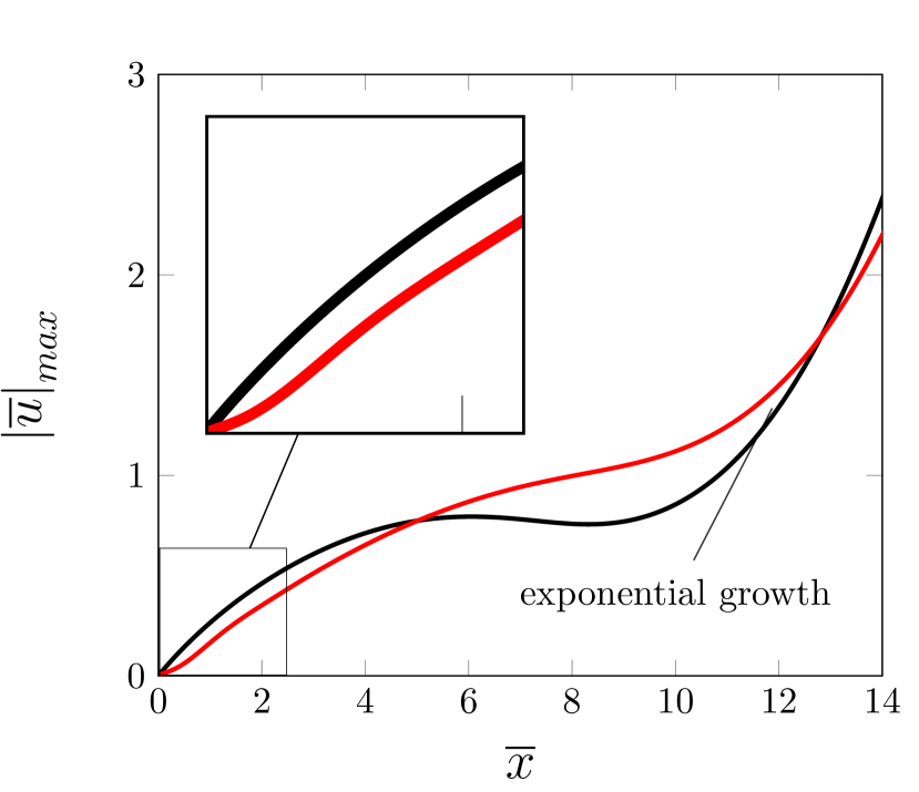
(c) $\kappa_{z}=0.007$, $k_{x}/k_{z}=0.31$.

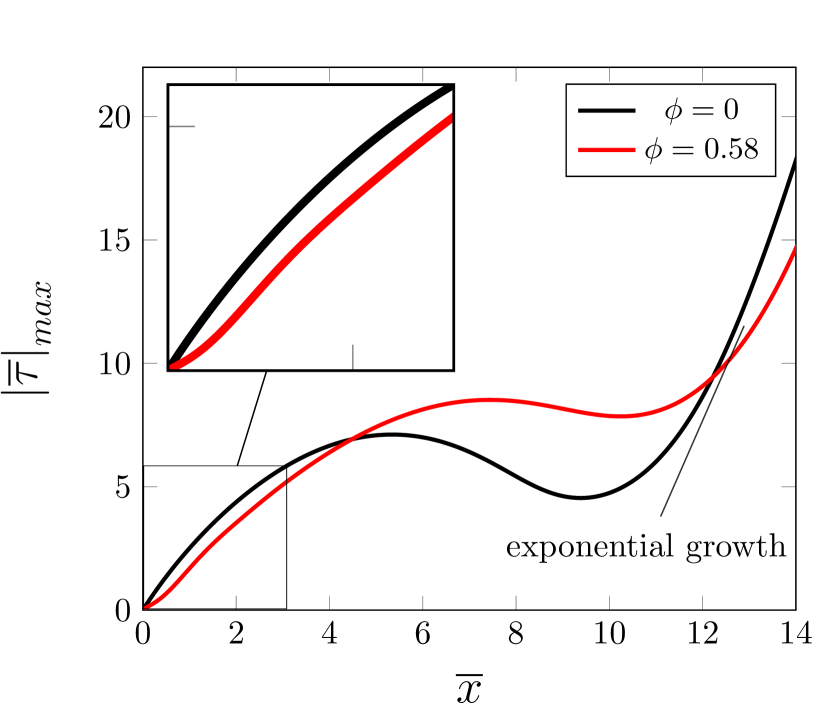
(d) $\kappa_{z}=0.007$, $k_{x}/k_{z}=0.31$.

Figure 5: Effect of the frequency on the attenuation streamwise velocity (figures 5(a), 5(b), 5(c)) and temperature 5(d)) for $\lambda_{z}^{\ast}=0.03\,$\mathrm{m}$$ ($\mathrm{R}_{\lambda}=418000$) at $\omega^{\ast}/2\pi=6730\,$\mathrm{Hz}$$ (5(a)), $\omega^{\ast}/2\pi=7570\,$\mathrm{Hz}$$ (5(b)) and $\omega^{\ast}/2\pi=8600\,$\mathrm{Hz}$$ (5(c)-5(d)). The solid ($\phi=0$) and porous ($\phi=0.58$) wall cases are represented with black and red curves, respectively.

(a) $\overline{x}_{2}=0.5$

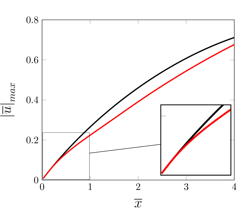
(b) $\overline{x}_{2}=1$

Figure 6: Effect of the adjustment-region length in the vicinity of the leading edge on the attenuation of the Klebanoff modes. $\overline{x}_{1}=0.005$ is kept constant and $\overline{x}_{2}$ is increased to 0.5 (figure 6(a)) and 1 (figure 6(b)). The solid ($\phi=0$) and porous ($\phi=0.58$) wall cases are represented by the black and red curves, respectively.

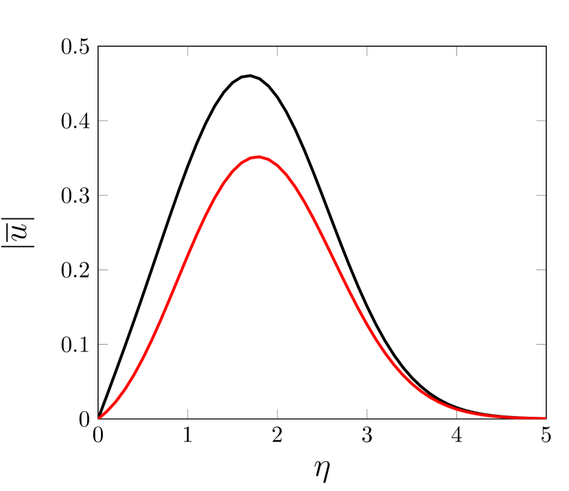
(a) Streamwise velocity at $\overline{x}=2$.

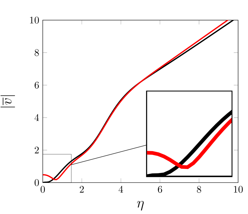
(b) Wall-normal velocity at $\overline{x}=2$.

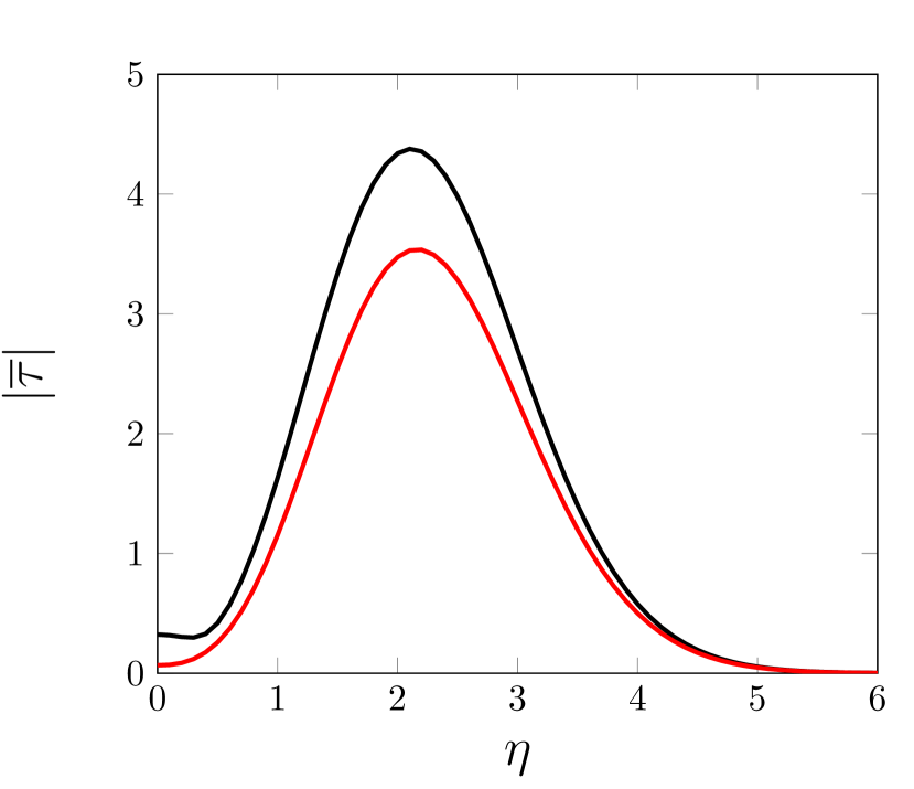
(c) Temperature at $\overline{x}=2$.

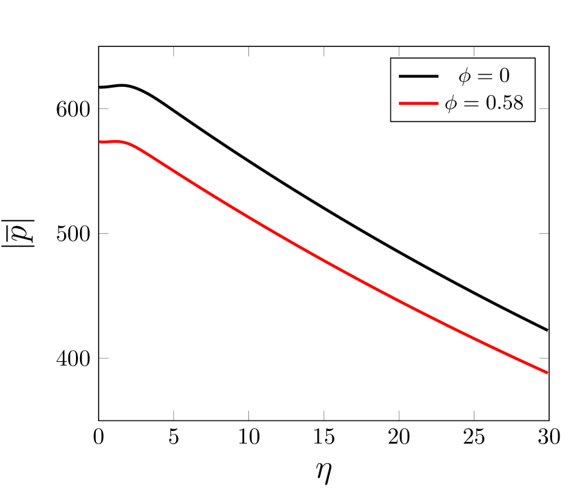
(d) Pressure at $\overline{x}=2$.

Figure 7: Wall-normal profiles of the streamwise velocity (7(a)), spanwise velocity (7(b)), temperature (7(c)), and pressure (7(d)) disturbances at $\overline{x}=2$ for $k_{z}/k_{x}=0.3$, $\kappa_{z}=0.007$, and $\mathrm{R}_{\lambda}=418000$. The solid ($\phi=0$) and porous ($\phi=0.58$) wall cases are represented with black and red curves, respectively.

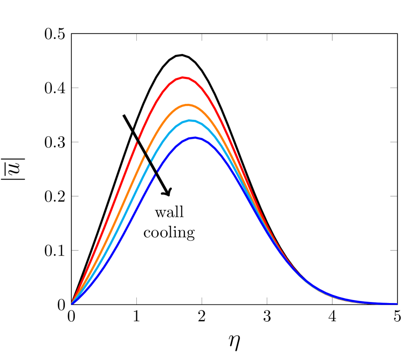
(a) solid wall

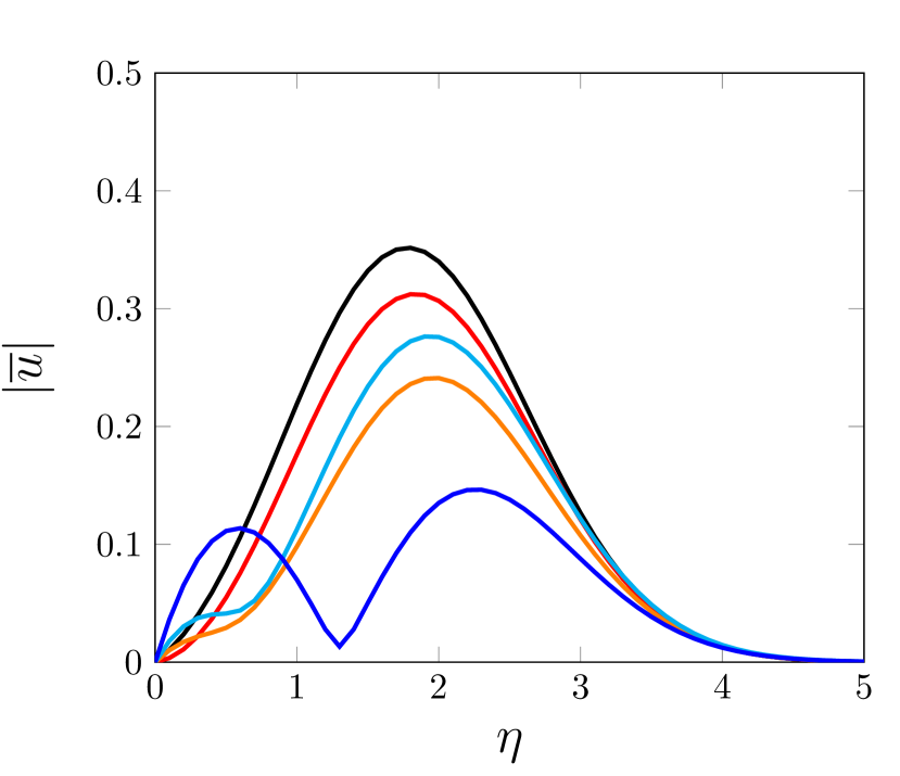
(b) porous wall

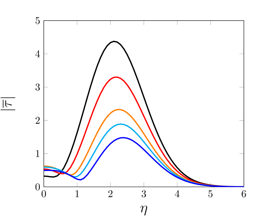
(c) solid wall

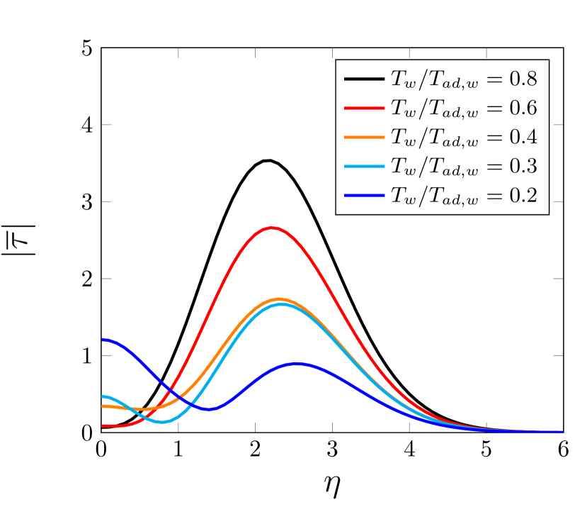
(d) porous wall

Figure 8: Effect of wall cooling on the streamwise velocity (top) and temperature (bottom) three-dimensional gust signatures profiles at $\overline{x}=2$ for $k_{x}/k_{z}=0.3$, $\kappa_{z}=0.007$, and $\mathrm{R}_{\lambda}=418000$. Solid and porous results are shown with solid and dashed lines, respectively.

The solution of the CLUBR equations for a flat-plate boundary layer is computed for a wide range of disturbance frequencies and spanwise wavelengths. Two wall-porosity conditions are considered: a solid plate with $\phi=0$ and a porous plate with $\phi=0.58$.

Our computations reveal that the wall porosity does not affect the growth of the Klebanoff modes for very low frequencies and very short spanwise wavelengths ($k_{x}\mathrm{R}_{\lambda}=\mathcal{O}\left({1}\right)$, $\kappa_{z}=\mathcal{O}\left({1}\right)$). Under these conditions, the spanwise viscous diffusion plays a significant role because $\lambda_{z}^{\ast}$ is comparable to the boundary-layer thickness $\delta^{\ast}$, which is typically a few millimeters (Laufer and Vrebalovich, 1960; Demetriades, 1985; Graziosi, 1999; Graziosi and Brown, 2002). The spectrum of free-stream disturbances is however wide and encompasses a wide range of spanwise wavelenghts and frequencies. We then investigate the response of the boundary layer to free-stream gusts with spanwise wavelengths that are larger than the boundary-layer thickness, i.e. $\lambda_{z}^{\ast}=0.03\,$\mathrm{m}$$ and $\mathrm{R}_{\lambda}=\mathrm{R}^{\ast}\lambda^{\ast}_{z}=418000$. As $k_{x}\mathrm{R}_{\lambda}$ increases and $\kappa_{z}$ decreases, the effect of the porous wall becomes relevant. Its response to increasing the disturbance frequency is reported in figures 5(a), 5(b), and 5(c), which show the downstream evolution of the peak of the streamwise velocity fluctuations, $\left|{\overline{u}}\right|_{max}$, for $\kappa_{z}=0.008,0.0075$ and $0.007$, respectively. Under these conditions, the scaled admittance $\overline{A}_{v}$ is $-8.82\cdot 10^{-4}+1.434\cdot 10^{-3}\ \mathrm{i}$. The growth of the Klebanoff modes is reduced by the porous wall up to about $\overline{x}=5$. The peak of the temperature fluctuations, shown in figure 5(d) for $\kappa_{z}=0.007$, is also reduced. The attenuation becomes more significant as $\omega^{\ast}$ increases and $\kappa_{z}$ decreases, meaning that the pores absorb and dissipate the energy of the Klebanoff modes when the spanwise diffusion is small. The effectiveness of the porous layer is expected to improve at frequencies higher than those considered here. However, increasing $k_{x}$ beyond 0.3 might lead to a regime for which the second-order perturbation discussed in §2.2 become important. The growth of the streamwise velocity and temperature fluctuations becomes exponential further downstream, where the receptivity of highly-oblique Tollmien-Schlichting waves sets in. This regime is studied in §3.2.

The results reported in figure 5 were computed by considering the leading-edge adjustment region given by equation (34) and extending between $\overline{x}_{1}=0.005$ and $\overline{x}_{2}=0.01$. The same case with $\kappa_{z}=0.007$ and $\mathrm{R}_{\lambda}=418000$ is computed for larger $\overline{x}_{2}$, i.e. $\overline{x}_{2}$=0.5 (figure 6(a)) and $\overline{x}_{2}$=1 (figure 6(b)). The growth of the Klebanoff modes is shown in figure 6. Extending the length of the adjustment region results in a delay of the attenuation. Albeit delayed, the damping of the Klebanoff modes is still appreciable in the region $\overline{x}\leq 4$.

More insights on the effect of wall porosity on the Klebanoff modes for $\kappa_{z}\ll 1$ can be inferred from the wall-normal profiles of the velocity components, the temperature and the pressure. The profiles for $\left|{\overline{u}}\right|$, $\left|{\overline{v}}\right|$, $\left|{\overline{\tau}}\right|$, and $\left|{\overline{p}}\right|$ at $\overline{x}=2$ for the case $\kappa_{z}=0.007$, $\mathrm{R}_{\lambda}=418000$ are shown in figure 7. The streamwise velocity, the temperature, and the pressure are markedly reduced by the porous wall. The peaks of $\left|{\overline{u}}\right|$ and $\left|{\overline{\tau}}\right|$ are decreased and slightly shifted farther from the wall. The wall-normal gradient of $\left|{\overline{u}}\right|$ is attenuated by the porous layer. The wall-normal velocity component $\left|{\overline{v}}\right|$ is enhanced in the proximity of the wall (inset of figure 7(b)), but is mostly unaffected at larger wall-normal locations. The spanwise velocity component (not shown) is unchanged, which is consistent with the spanwise momentum balance being independent of $\overline{u}$, $\overline{v}$, $\overline{\tau}$ and $\overline{p}$ when $\kappa_{z}\ll 1$ (RW07). The pressure distribution retains its shape and is uniformly attenuated when the wall is porous.

The results of figure 5 are computed at a fixed wall temperature ratio $T_{w}/T_{ad,w}=0.8$. As shown in the schematic of relation (36) of figure 4, the theory indicates that a lower wall temperature increases the range of $\omega^{\ast}$ and $\lambda_{z}^{\ast}$ for which the pressure fluctuations are effectively transduced into wall-normal velocity fluctuations. The wall-normal profiles for the boundary-layer fluctuations at $\mathrm{M}_{\infty}=6$, $\kappa_{z}=0.007$ and $\mathrm{R}_{\lambda}=418000$ are computed for five different wall temperature ratios $T_{w}/T_{ad,w}$ and reported in figure 8. The graphs in the top row show the $\left|{\overline{u}}\right|$-profiles over solid (figure 8(a)) and porous (figure 8(b)) flat plates. Wall cooling uniformly reduces the amplitude of the velocity and temperature fluctuations in the solid and porous cases.

In the solid-wall case, wall cooling causes the peak of the wall-normal profiles to shift farther from the wall, the wall-shear stress is attenuated, and the temperature fluctuations are reduced more than the velocity fluctuations, with the exception of the near-wall region where they slightly increase. The effect of wall cooling is more intense on the temperature fluctuations than on the velocity fluctuations when the wall-temperature ratio is reduced from 0.8 to 0.4. When the wall is porous, an inflection point appears close to the wall for $T_{w}/T_{ad,w}=0.4$, and a second shorter peak in the velocity distribution grows in the near-wall region between $T_{w}/T_{ad,w}=0.3$ and $T_{w}/T_{ad,w}=0.2$. Although the amplitude of the main velocity peak in the porous case is reduced by wall cooling, the wall-shear stress increases and the intensity of the secondary temperature peak, located at the wall, exceeds that of the main temperature peak.

3.2 Tollmien-Schlichting waves

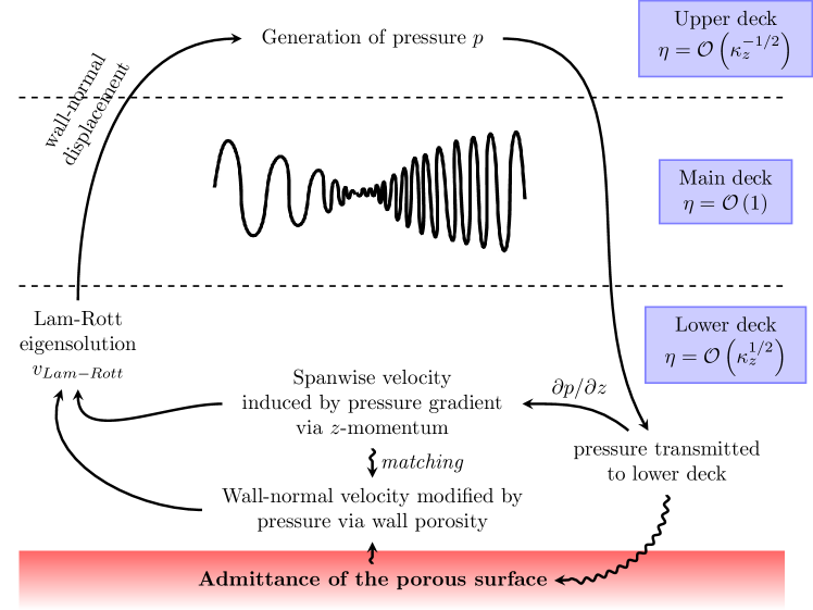
Figure 9: Schematic of triple-deck interactive regime of leading-edge receptivity mechanism in the presence of a porous surface. The thicknesses of the decks is out of scale.

For low $\kappa_{z}$ values, the initial algebraic growth of the compressible Klebanoff modes is followed downstream by the exponential growth of highly-oblique Tollmien-Schlichting (TS) waves, a receptivity mechanism first discovered by RW07. Numerical evidence of this receptivity mechanism is shown in figure 5 for $\overline{x}>6$, where the exponential growth occurs. Although the amplitude of the Klebanoff modes is attenuated, the porous wall enhances the initial amplitude of the TS waves, as also schematically illustrated in figure 4. Our numerical result confirms the experimental findings of Shiplyuk et al. (2004) and Lukashevich et al. (2018). The theoretical results of Michael and Stephen (2012) also reported a larger TS-wave growth rate, although the receptivity was not included in their analysis.

The mathematical framework utilized by RW07 to analyze this receptivity mechanism, based on the triple-deck formalism, is extended to include wall porosity. The objectives are to verify the numerical results and to gain further insight into the modified flow instability. As the theoretical analysis is valid for $\kappa_{z}\ll 1$, a small value of $\kappa_{z}=0.0005$ is chosen for a quantitative comparison between the theoretical results and the computational data obtained by solving the CLUBR equations.

The receptivity mechanism operates as follows. RW07 showed that the unsteady free-stream perturbations excite quasi three-dimensional Lam-Rott boundary-layer eigensolutions (Lam and Rott, 1960), which develop downstream together with the Klebanoff modes. Goldstein (1983) first discovered that these low-amplitude decaying eigensolutions, believed until then to be innocuous for the flow instability, can turn into exponentially growing TS waves. For relatively high-frequency acoustic oscillations, Goldstein (1983) proved that the wavelength shortening of these eigensolutions indeed causes the generation of a streamwise pressure gradient that is responsible for the instability. RW07 instead showed that, in the low-frequency regime proper of the Klebanoff modes, a spanwise pressure gradient is induced. This pressure gradient interferes with the viscous flow by engendering a spanwise velocity component. As this component reaches the order of magnitude of the streamwise and wall-normal velocity ones, a triple-deck interacting regime sets in and a spatially-growing oblique TS wave is triggered. This receptivity mechanism is similar to the leading-edge adjustment discovered by Goldstein (1983) in that the Lam-Rott eigensolution is central for the boundary-layer dynamics. Yet, it is different because the spanwise pressure gradient is responsible for triggering the instability, while the streamwise pressure gradient is negligible. The schematic in figure 9 illustrates these physical interactions. In the case of a porous wall, the wall-normal velocity near the wall is not only altered through continuity by the spanwise velocity generated by the induced spanwise pressure gradient, but also by the wall pressure via the admittance relationship (13a). The triple-deck theory has the advantage of revealing the physical mechanism responsible for engendering the first-mode growth, while this result is not achieved by performing finite-Reynolds-number stability analysis or by solving the complete Navier-Stokes equations.

The triple-deck analysis of RW07 is modified to investigate how a porous surface alters the dynamics of exponentially growing unstable waves. Analogously to RW07, an asymptotic eigensolution of the CLUBR equations is sought in the limits $\kappa_{z}\ll 1$ and $\overline{x}\gg 1$. The relevant class of eigensolutions is the one discovered by Lam and Rott (1960) (refer also to Ackerberg and Phillips (1972)). These eigensolutions are proportional to $\exp(-\hat{\psi}\overline{x}^{3/2})$, where $\hat{\psi}$ is an unknown complex eigenvalue (Ackerberg and Phillips, 1972; Goldstein, 1983). The eigensolutions are governed by the boundary-layer equations and the pressure disturbances need not be solved (LWG99). The boundary layer splits up into two decks: a main deck and a thin near-wall lower-deck. In the main deck, $\eta=\mathcal{O}(1)$ and

$$\left\{\overline{u},\overline{v},\overline{w},\overline{\tau}\right\}=\left\{\frac{F^{\prime\prime}(\eta)}{T},-\frac{3}{2}\hat{\psi}\sqrt{\overline{x}}F^{\prime}(\eta),0,-\frac{T^{\prime}(\eta)}{T}\right\}\exp(-\hat{\psi}\overline{x}^{3/2})+\ldots$$ (37)

satisfy the leading-order balance in the CLUBR equations. As shown by RW07, a triple-deck interactive regimes ensues because the wall-normal displacement induced downstream by the perturbation generates an unsteady pressure. This interactive regimes occurs where

$$\overline{x}=\mathcal{O}\left(\kappa_{z}^{-1}\right).$$ (38)

The decaying Lam-Rott perturbation evolves into a spatially growing, highly oblique TS wave at the locations specified by (38) when $k_{x}=\order{\mathrm{R}_{\lambda}^{-1/5}}$ or $\kappa_{z}=\order{\mathrm{R}_{\lambda}^{-2/5}}$. As the induced pressure disturbance now plays an active role, the porosity of the wall affects the flow field. The streamwise coordinate

$$x_{1}=\kappa_{z}\overline{x}=\mathcal{O}(1)$$ (39)

can be introduced because of (38) and $\kappa_{z}\ll 1$. An interactive triple-deck structure emerges, consisting of a lower deck $\eta=\mathcal{O}(\kappa_{z}^{1/2})$, a main deck $\eta=\mathcal{O}(1)$, and an upper deck $\eta=\mathcal{O}(\kappa_{z}^{-1/2})$.

In the main deck, the solution expands as

$$\left\{\overline{u},\overline{v},\overline{w},\overline{p},\overline{\tau}\right\}=\left\{u_{1}(x_{1},\eta),\kappa_{z}^{-1/2}v_{1}(x_{1},\eta),w_{1}(x_{1},\eta),\kappa_{z}^{-5/2}p_{1}(x_{1}),\tau_{1}(x_{1},\eta)\right\}E+\ldots$$ (40)

where

$$E=\exp\left(\frac{\mathrm{i}}{\kappa_{z}^{1/2}}\int_{0}^{\overline{x}}\alpha_{1}(x_{1})\mathrm{d}\breve{x}\right).$$ (41)

By substituting (40) into the CLUBR equations and by solving the resulting equations at leading order, one finds

$$\left\{u_{1},v_{1},w_{1},\tau_{1}\right\}=\left\{\mathcal{A}(x_{1})F^{\prime\prime}/T,-\mathrm{i}\alpha_{1}\mathcal{A}(x_{1})F^{\prime},p_{1}(x_{1})T/\left(\mathrm{i}\alpha_{1}F^{\prime}\right),-\mathcal{A}(x_{1})T^{\prime}/T\right\},$$ (42)

where $\mathcal{A}(x_{1})$ is an arbitrary function of $x_{1}$.

In the lower deck, we introduce $\underline{\eta}=\kappa_{z}^{-1/2}\eta=\mathcal{O}(1)$ and the leading-order solution is expressed as

$$\left\{\overline{u},\overline{v},\overline{w},\overline{\tau}\right\}=\left\{\overline{u}_{1}(x_{1},\underline{\eta}),\overline{v}_{1}(x_{1},\underline{\eta}),\kappa_{z}^{-1/2}\overline{w}_{1}(x_{1},\underline{\eta}),\kappa_{z}^{1/2}\overline{\tau}_{1}(x_{1},\underline{\eta})\right\}E+\ldots.\ \$$ (43)

Inserting (43) into the CLUBR equations yields

$$\left.\begin{array}[]{rl}\displaystyle\mathrm{i}\alpha_{1}\overline{u}_{1}+\frac{1}{T_{w}}\frac{\partial\overline{v}_{1}}{\partial\underline{\eta}}+\overline{w}_{1}=&0,\\ \vspace{-.2cm}\hfil\\ \displaystyle\mathrm{i}\left(-1+F^{\prime\prime}(0)\alpha_{1}\underline{\eta}\,\right)\overline{u}_{1}+\frac{F^{\prime\prime}(0)}{T_{w}}\overline{v}_{1}=&\displaystyle\frac{\mu_{w}}{2x_{1}T_{w}}\frac{\partial^{2}\overline{u}_{1}}{\partial\underline{\eta}^{2}},\\ \vspace{-.2cm}\hfil\\ \displaystyle\mathrm{i}\left(-1+F^{\prime\prime}(0)\alpha_{1}\underline{\eta}\,\right)\overline{w}_{1}=&\displaystyle T_{w}p_{1}+\frac{\mu_{w}}{2x_{1}T_{w}}\frac{\partial^{2}\overline{w}_{1}}{\partial\underline{\eta}^{2}}.\\ \end{array}\right\}$$ (44)

The pressure $p_{1}$ in the lower deck is solely a function of $x_{1}$. Enforcing the no-slip condition on the streamwise and spanwise velocity components ($\overline{u}_{1}=0$, $\overline{w}_{1}=0$) in (44) yields

$$\left.\begin{array}[]{rl}\displaystyle\left.\frac{\partial\overline{v}_{1}}{\partial\underline{\eta}}\right|_{\underline{\eta}=0}=&0,\\ \vspace{-.2cm}\hfil\\ F^{\prime\prime}(0)\left.\overline{v}_{1}\right|_{\underline{\eta}=0}=&\displaystyle\frac{\mu_{w}}{2x_{1}}\left.\frac{\partial^{2}\overline{u}_{1}}{\partial\underline{\eta}^{2}}\right|_{\underline{\eta}=0},\\ \vspace{-.2cm}\hfil\\ \displaystyle T_{w}p_{1}+\frac{\mu_{w}}{2x_{1}T_{w}}\left.\frac{\partial^{2}\overline{w}_{1}}{\partial\underline{\eta}^{2}}\right|_{\underline{\eta}=0}=&0.\\ \end{array}\right\}$$ (45)

By differentiation of the first equation in (44) and by use of the second and third equations in (45), one obtains

$$\frac{2\mathrm{i}x_{1}\alpha_{1}F^{\prime\prime}(0)}{\mu_{w}}\left.\overline{v}_{1}\right|_{\underline{\eta}=0}+\frac{1}{T_{w}}\left.\frac{\partial^{3}\overline{v}_{1}}{\partial\underline{\eta}^{3}}\right|_{\underline{\eta}=0}-\frac{2x_{1}T_{w}^{2}}{\mu_{w}}p_{1}=0.$$ (46)

Eliminating $p_{1}$ from (44) shows that $\overline{v}_{1}$ satisfies

$$\left[\frac{\partial^{2}}{\partial\underline{\eta}^{2}}-\frac{2\mathrm{i}x_{1}T_{w}}{\mu_{w}}\left(F^{\prime\prime}(0)\alpha_{1}\underline{\eta}-1\right)\right]\frac{\partial^{2}\overline{v}_{1}}{\partial\underline{\eta}^{2}}=0,$$ (47)

which has solution

$$\frac{\partial\overline{v}_{1}}{\partial\underline{\eta}}=\int_{\eta_{0}}^{\hat{\eta}}\mbox{Ai}(\breve{\eta})\mathrm{d}\breve{\eta},$$ (48)

where

$$\widehat{\eta}=\left(2\mathrm{i}F^{\prime\prime}(0)\alpha_{1}x_{1}T_{w}/\mu_{w}\right)^{1/3}\underline{\eta}+\eta_{0},\quad\eta_{0}=-(\alpha_{1}F^{\prime\prime}(0))^{-1}\left(2\mathrm{i}F^{\prime\prime}(0)\alpha_{1}x_{1}T_{w}/\mu_{w}\right)^{1/3}.$$ (49)

Differentiation of (48) yields

$$\left.\frac{\partial^{3}\overline{v}_{1}}{\partial\underline{\eta}^{3}}\right|_{\underline{\eta}=0}=\left(\frac{2\mathrm{i}F^{\prime\prime}(0)\alpha_{1}x_{1}T_{w}}{\mu_{w}}\right)^{2/3}\mbox{Ai}^{\prime}(\eta_{0}).$$ (50)

At the wall, the wall-normal velocity component and the pressure are related through (13a) and (13b). By use of (39), (40), and (43), it follows that

$$\left.\overline{v}_{1}\right|_{\underline{\eta}=0}=\frac{A_{v}}{\kappa_{z}^{2}}\left(\frac{k_{x}}{2x_{1}R_{\lambda}}\right)^{1/2}\left.\overline{p}\right|_{\underline{\eta}=0}=\frac{\overline{A}_{v}p_{1}}{\kappa_{z}^{2}\left(2x_{1}\right)^{1/2}}.$$ (51)

In the case of oblique TS waves, for which $\kappa_{z}\ll 1$ and $\overline{x}\gg 1$, an admittance $A_{v}=\mathcal{O}\left(R_{\lambda}^{-1/2}k_{x}^{-3/2}\right)$ $\left(\overline{A}_{v}=\mathcal{O}(\kappa_{z}^{2})\ll 1\right)$ is sufficient to alter the dynamics of the growing waves. A scaled admittance $\widetilde{A}_{v}=\overline{A}_{v}\kappa_{z}^{-2}=\mathcal{O}(1)$ is defined, and thus

$$\left.\overline{v}_{1}\right|_{\underline{\eta}=0}=\frac{\widetilde{A}_{v}p_{1}}{\left(2x_{1}\right)^{1/2}}.$$ (52)

The wall-normal velocity component and the pressure at the wall can now be determined. By substituting (52) into (46), it follows that

$$\left(\mathrm{i}\alpha_{1}F^{\prime\prime}(0)-\frac{(2x_{1})^{1/2}T_{w}^{2}}{\widetilde{A}_{v}}\right)\left.\overline{v}_{1}\right|_{\underline{\eta}=0}+\frac{\mu_{w}}{2x_{1}T_{w}}\left.\frac{\partial^{3}\overline{v}_{1}}{\partial\underline{\eta}^{3}}\right|_{\underline{\eta}=0}=0.$$ (53)

By substitution of (50) into (53), an expression for the wall-normal velocity at the wall is found

$$\left.\overline{v}_{1}\right|_{\underline{\eta}=0}=\frac{\left(2\mathrm{i}F^{\prime\prime}(0)\alpha_{1}x_{1}T_{w}/\mu_{w}\right)^{2/3}\mbox{Ai}^{\prime}(\eta_{0})\mu_{w}\widetilde{A}_{v}}{2x_{1}T_{w}\left(T_{w}^{2}(2x_{1})^{1/2}-\mathrm{i}\widetilde{A}_{v}\alpha_{1}F^{\prime\prime}(0)\right)}.$$ (54)

By use of (52), the pressure in the lower deck is obtained

$$\left.\overline{p}_{1}\right|_{\underline{\eta}=0}=\frac{\left(2\mathrm{i}F^{\prime\prime}(0)\alpha_{1}x_{1}T_{w}/\mu_{w}\right)^{2/3}\mbox{Ai}^{\prime}(\eta_{0})\mu_{w}}{(2x_{1})^{1/2}T_{w}\left(T_{w}^{2}(2x_{1})^{1/2}-\mathrm{i}\widetilde{A}_{v}\alpha_{1}F^{\prime\prime}(0)\right)}.$$ (55)

Matching $\partial\overline{v}_{1}/\partial\underline{\eta}$ in (48) with the main-deck solution (42) yields

$$\int_{\eta_{0}}^{\infty}\mbox{Ai}(\breve{\eta})\mathrm{d}\breve{\eta}=-\mathrm{i}F^{\prime\prime}(0)\alpha_{1}\mathcal{A}(x_{1}).$$ (56)

In the upper deck, the appropriate wall-normal variable is $\widetilde{\eta}=\kappa_{z}^{1/2}\eta=\mathcal{O}(1)$, and the solution expands as

$$\left\{\overline{u},\overline{v},\overline{w},\overline{p},\overline{\tau}\right\}=\left\{\kappa_{z}^{1/2}\widetilde{u}_{1}(x_{1},\widetilde{\eta}),\kappa_{z}^{-1/2}\widetilde{v}_{1}(x_{1},\widetilde{\eta}),\widetilde{w}_{1}(x_{1},\widetilde{\eta}),\kappa_{z}^{-5/2}\widetilde{p}_{1}(x_{1},\widetilde{\eta}),0\right\}E+\ldots.$$ (57)

Inserting (57) into the CLUBR equations leads to

$$\mathrm{i}\alpha_{1}\widetilde{u}_{1}+\frac{\partial\widetilde{v}_{1}}{\partial\widetilde{\eta}}+\widetilde{w}_{1}=0,\quad\widetilde{u}_{1}=0,\quad\mathrm{i}\alpha_{1}\widetilde{v}_{1}+\frac{1}{2x_{1}}\frac{\partial\widetilde{p}_{1}}{\partial\widetilde{\eta}}=0,\quad\mathrm{i}\alpha_{1}\widetilde{w}_{1}-\widetilde{p}_{1}=0.$$ (58)

These equations can be reduced to a Laplace equation for $\widetilde{p}_{1}$,

$$\frac{\partial^{2}\widetilde{p}_{1}}{\partial\widetilde{\eta}^{2}}-2x_{1}\widetilde{p}_{1}=0,$$

whose solution is $\widetilde{p}_{1}=p_{1}(x_{1})\mbox{exp}\left(-\sqrt{2x_{1}}\widetilde{\eta}\right)$. The vertical velocity behaves as $\widetilde{v}_{1}\rightarrow-\mathrm{i}p_{1}/(\alpha_{1}\sqrt{2x_{1}})$ for $\widetilde{\eta}\rightarrow 0$, and matching it with the main-deck solution yields

$$p_{1}=\alpha_{1}^{2}\mathcal{A}(x_{1})\sqrt{2x_{1}}.$$ (59)

Eliminating $\mathcal{A}$ from (56) and (59) yields

$$\Delta(x_{1},\alpha_{1})\equiv\int_{\eta_{0}}^{\infty}\mbox{Ai}(\breve{\eta})\mathrm{d}\breve{\eta}-\left(\frac{\mu_{w}}{2\alpha_{1}x_{1}T_{w}}\right)^{1/3}\frac{\left(\mathrm{i}F^{\prime\prime}(0)\right)^{5/3}\mbox{Ai}^{\prime}(\eta_{0})}{\mathrm{i}\widetilde{A}_{v}\alpha_{1}F^{\prime\prime}(0)-(2x_{1})^{1/2}T_{w}^{2}}=0,$$ (60)

which is the dispersion relation that determines the complex wavenumber $\alpha_{1}=\alpha_{1}(x_{1})$.

The admittance $\widetilde{A}_{v}$ in (60) is absent in the dispersion relation as $x_{1}\rightarrow 0$, so $\mbox{Ai}^{\prime}(\eta_{0})\rightarrow 0$ as $x_{1}\rightarrow 0$. It follows from (54) that $v_{1}$ goes to zero at the wall as $x_{1}\rightarrow 0$ and the Lam-Rott eigensolutions are therefore not influenced by the porosity at leading order. Equation (60) reduces to the dispersion relation found by RW07 for a solid wall when $\widetilde{A}_{v}=0$. The Airy function and its derivative are computed by an in-house code, based on the method of Gil et al. (2001). The growth rate and the wavenumber are given by $-\imaginary(\alpha_{1})/\kappa_{z}^{1/2}$ and $\real(\alpha_{1})/\kappa_{z}^{1/2}$, respectively, and are also found numerically from the CLUBR equations as $\real(\overline{u}_{\overline{x}}/\overline{u})$ and $\imaginary(\overline{u}_{\overline{x}}/\overline{u})$ (where the subscript $\overline{x}$ indicates the derivative).

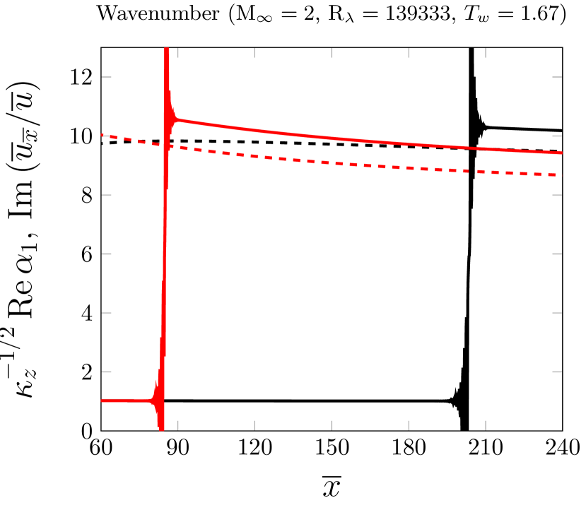
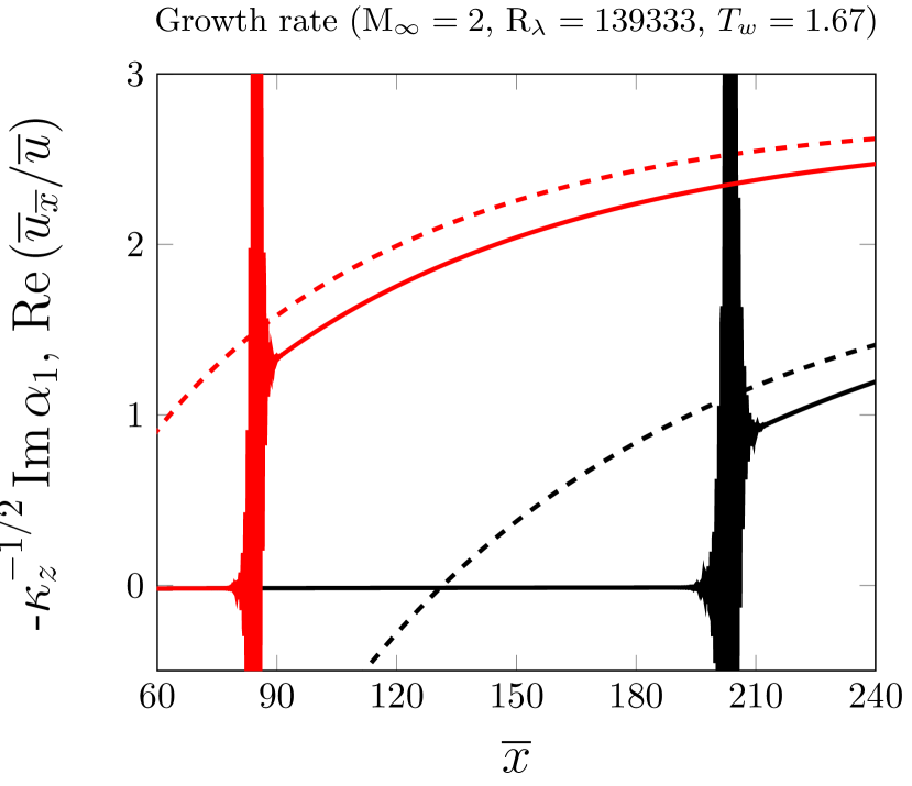
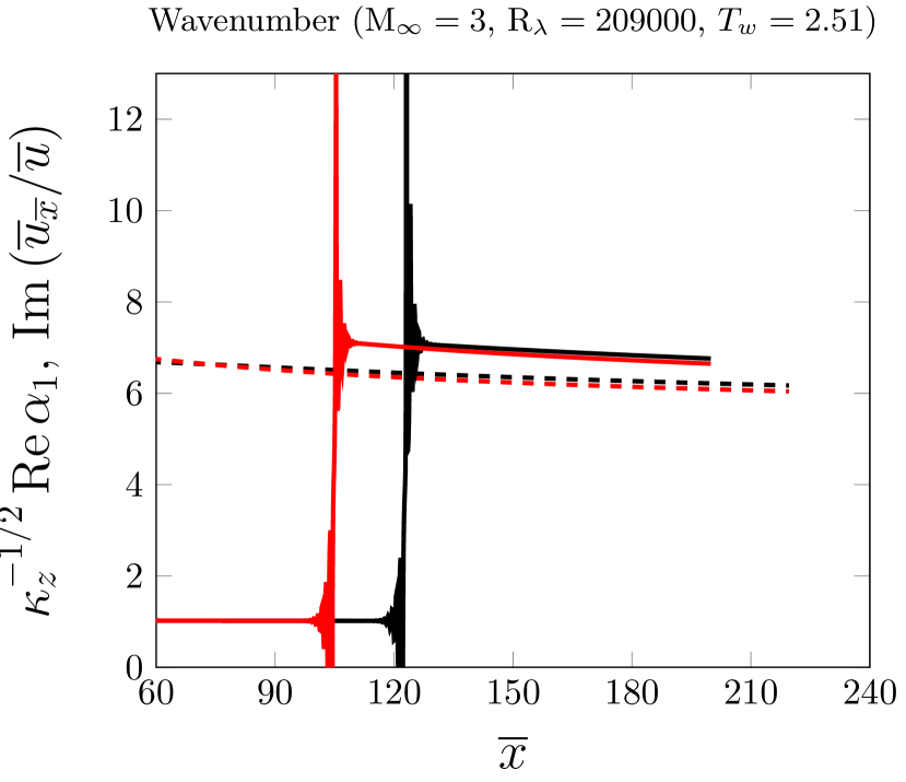
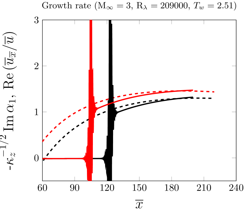
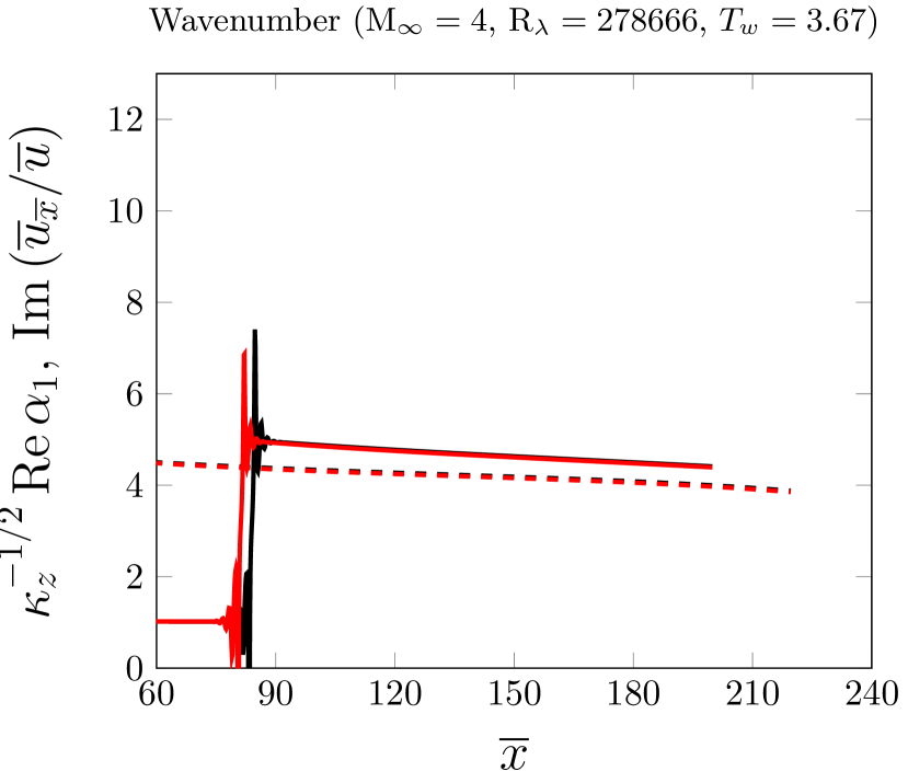
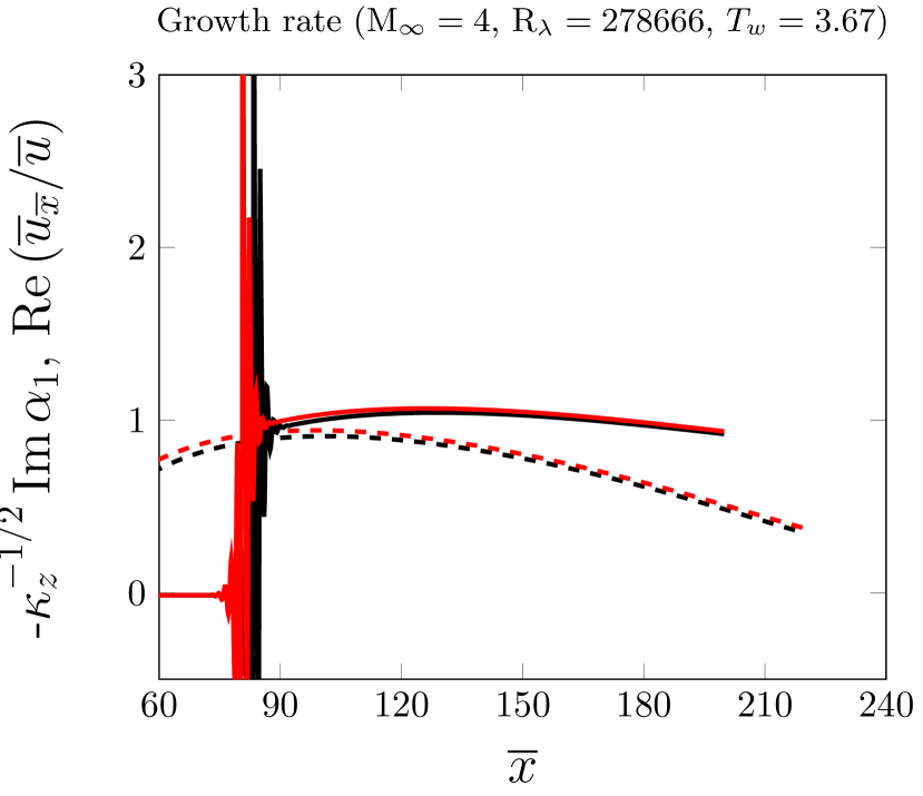
Figure 10: Onset of the oblique TS waves far downstream for $\kappa_{z}=0.0005$ on solid (black) and porous (red) walls. The solid lines indicate the boundary-region solutions and the dashed lines denote the triple-deck solutions. The three free-stream conditions at different Mach numbers are simulated by varying the free-stream velocity $U_{\infty}^{\ast}$ on adiabatic wall conditions.

The solutions have been first computed for $\widetilde{A}_{v}=\mathcal{O}(1)$ and $\mathrm{M}_{\infty}$=2, 3, and 4 on an adiabatic wall. The free-stream disturbances are assumed to be the same in all cases and a porous wall of fixed $R^{\ast}$, $\phi$ and $H^{\ast}$ is considered. The Mach number and Reynolds number vary together as the free-stream velocity $U_{\infty}^{*}$ increases. The wavenumber and growth rate of the CLUBR solutions and the triple-deck solutions are compared in figure 10 for $\kappa_{z}=0.0005$ at $\mathrm{M}_{\infty}=2$, 3 and 4. The triple-deck analysis predicts the growth rate and the wavenumber of the TS instability in the solid and the porous cases, while the CLUBR solutions also give the onset of the instability. The growth rate, which is mildly negative upstream, suddenly increases as the TS waves are triggered, while the wavenumber settles to an almost constant value. The agreement between the CLUBR solutions (solid lines) and the triple-deck solutions (dashed lines) improves as the Mach number increases. The porous wall enhances the TS-wave growth rate and shifts the onset of the instability upstream, while the wavenumber is unaffected. The impact of the porous wall, however, diminishes as the Reynolds and Mach numbers increase with the free-stream velocity. For the flow conditions studied in figure 10, no effect of the porous wall is found at $\mathrm{M}_{\infty}=6$.

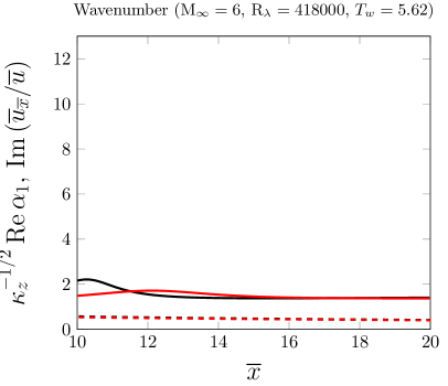
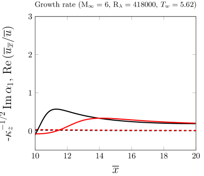
Figure 11: Onset of the oblique TS waves for $\kappa_{z}=0.007$ on solid (black) and porous (red) walls. The solid lines indicate the boundary-region solutions and the dashed lines the triple-deck solutions. The results are computed for the flow conditions discussed in §3.1: $\mathrm{M}_{\infty}=6$, $T_{w}=5.62$ and $\kappa_{z}=0.007$.

The case investigated in §3.1 is also studied ($\mathrm{M}_{\infty}=6$, $\kappa_{z}=0.007$, $T_{w}=0.8T_{ad,w}=5.62$, $\widetilde{A}_{v}=-18.00+29.26\ \mathrm{i}$). As per definition (39), the onset of the TS waves shifts upstream over both the porous and the solid surfaces when $\kappa_{z}$ increases slightly. The boundary-region and the triple-deck results, shown in figure 11, still show a satisfactory agreement for a relatively larger $\kappa_{z}$ and $\overline{x}>14$. The porous wall has an intense effect on the growth rate before the exponential growth of the TS waves sets in. Once the TS-wave growth is established, the effect of porosity is mild.

3.3 Effect of wall curvature at moderate Görtler number

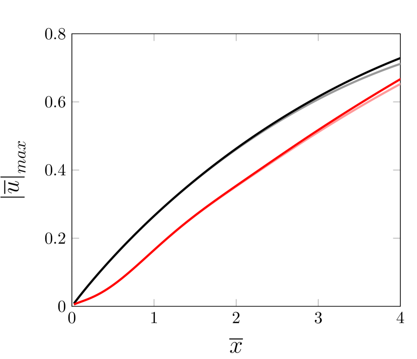
(a) $\mathrm{G}=2.41$.

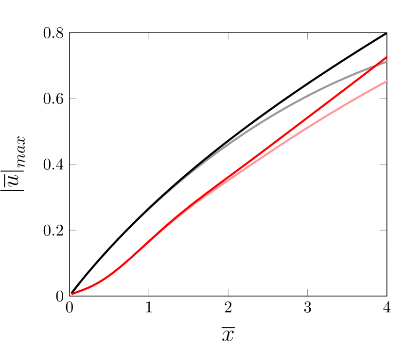
(b) $\mathrm{G}=12$.

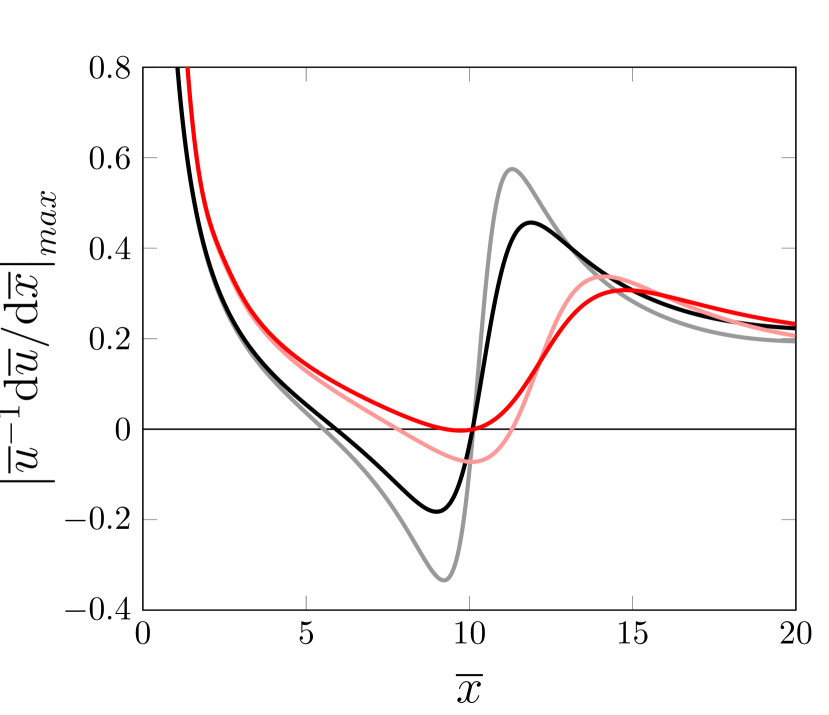
(c) $\mathrm{G}=2.41$.

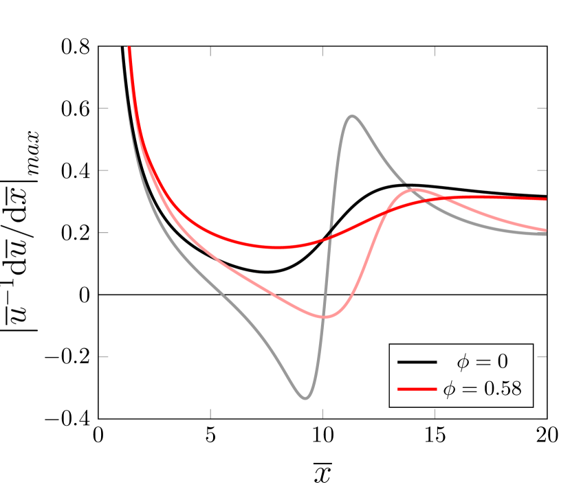
(d) $\mathrm{G}=12$.

Figure 12: Effect of the porous wall on a boundary layer $\mathrm{G}=\order{1}$ for $\kappa_{z}=0.007$, $\mathrm{R}_{\lambda}=418000$ and $\mathrm{M}_{\infty}=6$. The black and red curves refer to the solid and porous cases, respectively. The curves for the flat-plate case $\mathrm{G}=0$ are drawn in light colors.

The combined effect of wall porosity and wall curvature is considered. As proved by Hall (1983), in the limit of large Reynolds number and large curvature radius, the curvature does not affect the base flow and the centrifugal effects are distilled in two terms in the wall-normal momentum boundary-region equation (65) that are proportional to the Görtler number

$$\mathrm{G}=\frac{1}{r_{c}}\left(\frac{\mathrm{R_{\lambda}}}{k_{x}^{3}}\right)^{1/2},$$ (61)

where $r_{c}=r_{c}^{\ast}/\lambda_{z}^{\ast}$ is the scaled wall curvature radius (Viaro and Ricco, 2019a). The evolution of the boundary-layer perturbations was computed for $\kappa_{z}=0.007$, $\mathrm{R}_{\lambda}=418000$, $\mathrm{M}_{\infty}=6$ and two different Görtler numbers, $\mathrm{G}=2.41$ and $\mathrm{G}=12$, which correspond to $r_{c}=100$ and $r_{c}=20$, respectively. Under these conditions, the effect of curvature enhances the growth of the velocity disturbances compared to the flat-plate case. Since both $\mathrm{M}_{\infty}$ and $k_{x}\mathrm{R}_{\lambda}$ are relatively high, the onset of exponentially-growing Görtler vortices was not observed (Viaro and Ricco, 2019b). The downstream growth of $|\overline{u}|_{max}$ is shown in figures 12(a) and 12(b). The flat-plate ($\mathrm{G}=0$) results are plotted in light colors for comparison. The fluctuations on the concave plate are enhanced downstream of $\overline{x}=3$ ($\mathrm{G}=2.41$) and $\overline{x}=2$ ($\mathrm{G}=12$) with respect to those on the flat plate. The porous wall reduces the amplitude of the velocity disturbances with the centrifugal effects during their initial evolution, up to about $\overline{x}=4$. Flows with higher Görtler numbers were not investigated as values of $r_{c}<20$ might invalidate the hypothesis $r_{c}\gg\delta$.

The growth rate of $|\overline{u}|$ is shown in figures 12(c) and 12(d). Although the amplitude of $\left|{\overline{u}}\right|_{max}$ is reduced up to $\overline{x}=4$, the porous wall enhances its growth downstream of $\overline{x}=2$ up to $\overline{x}=10$ and attenuates it further downstream. Additional research is necessary to evince the effect of nonlinearity at these downstream locations because the magnitude of the fluctuations may be too large for the nonlinear interactions to be considered negligible.

4 Conclusions

The effect of regular-microstructure porous coatings on the receptivity of supersonic pre-transitional boundary layers to free-stream vortical disturbances has been studied. We have focused on the downstream evolution of Klebanoff modes over flat and concave surfaces and Tollmien-Schlichting waves generated by the external perturbations. We have used asymptotic and numerical methods to study these low-frequency disturbances in the limits of large Reynolds number and small amplitude.

The downstream development of the Klebanoff modes is largely unaffected by the wall porosity when the spanwise wavelength of the oncoming perturbation is of the same order of magnitude of the boundary-layer thickness. As either the frequency or the spanwise wavelength of the disturbances increases, the wall-normal velocity and the pressure interact at the wall and the boundary-layer streamwise velocity and temperature fluctuations are attenuated. This beneficial effect is enhanced further by wall cooling.

The growth rate of Tollmien-Schlichting waves, triggered by a leading-edge adjustment mechanism, is enhanced by the wall porosity, and the location of instability moves upstream. These waves are the first modes of compressible instability, so this finding confirms previous experimental results. A triple-deck asymptotic analysis quantitatively confirms the numerical results and reveals how the physical mechanism of instability is altered in the presence of wall porosity.

The porous layer also reduces the amplitude of the streaks over concave surfaces during their initial development and the growth rate of the streamwise velocity fluctuations further downstream.

The present work has focused on the linear response of boundary layers over porous walls to a monochromatic vortical disturbance. The full spectrum of free-stream disturbances, including acoustic and temperature fluctuations, and the nonlinear interaction of different modes should be considered in a more realistic context. Some of these aspects have been investigated by Zhang et al. (2011) and Xu et al. (2017, 2020). We plan to investigate the effect of wall porosity on the nonlinear compressible flows studied by Marensi et al. (2017) and to include higher-frequency second-mode instability in the analysis (Goldstein and Ricco, 2018). Another important avenue for research is the impact of wall porosity on the secondary instability and on the final stages of transition with the objective of precisely assessing how the porous wall influences the location of transition.

Our theoretical and numerical results require further numerical and experimental validation. Direct numerical simulations and wind tunnel or in-flight measurements of the receptivity of supersonic boundary layers to free-stream vortical disturbances remain ambitious challenges. We hope our study will stimulate further research on the boundary-layer control via porous surfaces.

Appendix A Validation of the laminar base-flow computation

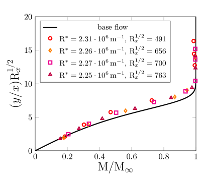
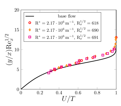
Figure 13: Comparison of our base-flow numerical solution (4) (solid lines) with the hot-wire data by Graziosi [1999, pp. 85-110] for $\mathrm{M}_{\infty}=3$, $\mathrm{Pr}=0.72$, and $T_{w}/T_{ad,w}=1.1$.

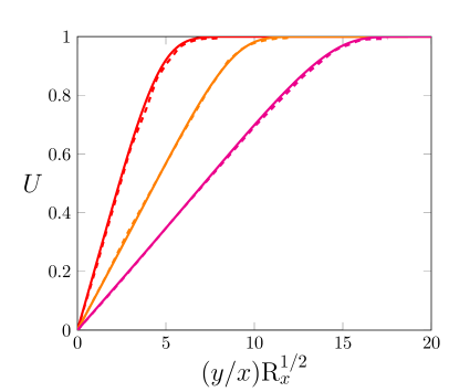
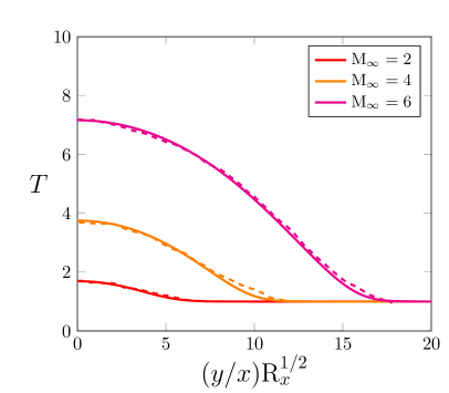
Figure 14: Comparison of our base-flow numerical solutions (4) (solid lines) with the numerical results by van Driest [1952, pp. 40-41] (dashed lines) for a boundary layer over an adiabatic flat plate ($\mathrm{Pr}=0.75$).

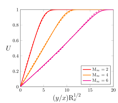
Figure 15: Comparison of our base-flow numerical solutions (4) (solid lines) with the numerical results by Stewartson [1964, p. 40] (dashed lines) for a boundary layer over an adiabatic flat plate ($\mathrm{Pr}=1.0$).

Our numerical solutions (4) of the base-flow system (6) are compared to numerical and experimental data available in the literature, retrieved by the authors by using an image-digitizing software. The numerical profiles are plotted versus the similarity variable

$$\widetilde{\eta}=\frac{y}{x}\mathrm{R}_{x}^{1/2}=2^{1/2}\int_{0}^{\eta}T\left(\breve{\eta}\right)\mathrm{d}\breve{\eta},$$ (62)

where $\mathrm{R}_{x}=U_{\infty}^{\ast}x^{\ast}/\nu_{\infty}^{\ast}$.

Our numerical solutions are first compared in figure 13 with the hot-wire data by [Graziosi, 1999, pp. 85-110] (refer also to Graziosi and Brown [2002]) for $\mathrm{M}_{\infty}=3$, $\mathrm{Pr}=0.72$, $T_{w}/T_{ad,w}=1.1$ and at different unit Reynolds numbers $\mathrm{R}^{\ast}=U_{\infty}^{\ast}/\nu_{\infty}^{\ast}$ and streamwise locations $\mathrm{R}_{x}^{1/2}$. Our solutions (solid lines), plotted against the local Mach number $\mathrm{M}/\mathrm{M}_{\infty}=U/T^{1/2}$ in figure 13a, show a satisfactory agreement with the experimental data. Other experimental data at fixed $\mathrm{R}^{\ast}$, plotted against $U/T$ and shown in figure 13b, show excellent agreement for $3\leq\widetilde{\eta}\leq 7$ and adequate agreement for $7\leq\widetilde{\eta}\leq 10$ ($\rho T=1$ for a perfect gas has been used to convert $\rho U$ given by Graziosi and Brown [2002]).

Our velocity and temperature profiles (4) (solid lines) and those computed by van Driest [1952, pp. 40-41] (dashed lines) for a boundary layer over an adiabatic plate with $\mathrm{Pr}=0.75$ are shown in figure 14. Results were generated by modelling the dynamic viscosity with Sutherland’s law $\mu=T^{3/2}(1+\chi)/(T+\chi)$, where $\chi=0.505$, as in van Driest [1952]. A good agreement is found for both the velocity (left) and temperature (right) profiles at all the Mach numbers.

Figure 15 shows that good agreement is also obtained between our solutions and the velocity profiles by Stewartson [1964, p. 40] for a boundary layer with $\mathrm{Pr}=1$ flowing over an adiabatic plate. The dynamic viscosity was computed by using the power law $\mu=T^{n}$, where $n=0.76$.

Appendix B The compressible linearized unsteady boundary region equations

In this appendix, the CLUBR equations, derived by RW07 and Viaro and Ricco [2019a], are reported.

• Continuity equation

  $$\begin{split}\frac{\eta_{c}T^{\prime}}{2\overline{x}T}\overline{u}+\frac{\partial\overline{u}}{\partial\overline{x}}-\frac{\eta_{c}}{2\overline{x}}\frac{\partial\overline{u}}{\partial\eta}-\frac{T^{\prime}}{T^{2}}\overline{v}+\frac{1}{T}\frac{\partial\overline{v}}{\partial\eta}+\overline{w}&\\ +\left(\frac{\mathrm{i}}{T}-\frac{FT^{\prime}}{2\overline{x}T^{2}}\right)\overline{\tau}+\frac{F^{\prime}}{T}\frac{\partial\overline{\tau}}{\partial\overline{x}}+\frac{F}{2\overline{x}T}\frac{\partial\overline{\tau}}{\partial\eta}&=0.\end{split}$$ (63)

• Streamwise momentum equation

  $$\begin{split}\left(-\mathrm{i}-\frac{\eta_{c}F^{\prime\prime}}{2\overline{x}}+\kappa_{z}^{2}\mu T\right)\overline{u}+F^{\prime}\frac{\partial\overline{u}}{\partial\overline{x}}+\left(-\frac{F}{2\overline{x}}-\frac{\mu^{\prime}T^{\prime}}{2\overline{x}T}+\frac{\mu T^{\prime}}{2\overline{x}T^{2}}\right)\frac{\partial\overline{u}}{\partial\eta}&\\ -\frac{\mu}{2\overline{x}T}\frac{\partial^{2}\overline{u}}{\partial\eta^{2}}+\frac{F^{\prime\prime}}{T}\overline{v}+\left(\frac{FF^{\prime\prime}}{2\overline{x}T}-\frac{\mu^{\prime\prime}T^{\prime}F^{\prime\prime}}{2\overline{x}T}+\frac{\mu^{\prime}T^{\prime}F^{\prime\prime}}{2\overline{x}T^{2}}-\frac{\mu^{\prime}F^{\prime\prime\prime}}{2\overline{x}T}\right)\overline{\tau}-\frac{F^{\prime\prime}}{2\overline{x}T}\frac{\partial\overline{\tau}}{\partial\eta}&=0.\end{split}$$ (64)

• Wall-normal momentum equation

  $$\begin{split}\frac{1}{\left(2\overline{x}\right)^{2}}\left(TF+\eta_{c}\left(FT^{\prime}-TF^{\prime}\right)-\eta_{c}^{2}TF^{\prime\prime}\right)\overline{u}+\frac{\mu^{\prime}T^{\prime}}{3\overline{x}}\frac{\partial\overline{u}}{\partial\overline{x}}&\\ +\frac{1}{12\overline{x}^{2}}\left[\mu+\eta_{c}T\left(\frac{\mu}{T}\right)^{\prime}\right]\frac{\partial\overline{u}}{\partial\eta}+\frac{\eta_{c}\mu}{12\overline{x}^{2}}\frac{\partial^{2}\overline{u}}{\partial\eta^{2}}&\\ -\frac{\mu}{6\overline{x}}\frac{\partial^{2}\overline{u}}{\partial\overline{x}\partial\eta}+\left(-\mathrm{i}+\frac{F^{\prime}}{2\overline{x}}-\frac{T^{\prime}F}{2\overline{x}T}+\frac{\eta_{c}F^{\prime\prime}}{2\overline{x}}+\kappa_{z}^{2}\mu T\right)\overline{v}+F^{\prime}\frac{\partial\overline{v}}{\partial\overline{x}}&\\ +\left(-\frac{F}{2\overline{x}}-\frac{2\mu^{\prime}T^{\prime}}{3\overline{x}T}+\frac{2\mu T^{\prime}}{3\overline{x}T^{2}}\right)\frac{\partial\overline{v}}{\partial\eta}-\frac{2\mu}{3\overline{x}T}\frac{\partial^{2}\overline{v}}{\partial\eta^{2}}+\frac{\mu^{\prime}T^{\prime}}{3\overline{x}}\overline{w}-\frac{\mu}{6\overline{x}}\frac{\partial\overline{w}}{\partial\eta}&\\ +\frac{1}{\left(2\overline{x}\right)^{2}}\left[\eta_{c}\left(FF^{\prime}\right)^{\prime}-FF^{\prime}-\frac{T^{\prime}F^{2}}{T}-\mu^{\prime}F^{\prime\prime}-\eta_{c}T\left(\frac{\mu^{\prime}F^{\prime\prime}}{T}\right)^{\prime}+\frac{4}{3}\left(\frac{\mu^{\prime}T^{\prime}F}{T}\right)^{\prime}\right]\overline{\tau}&\\ -\frac{\mu^{\prime}F^{\prime\prime}}{2\overline{x}}\frac{\partial\overline{\tau}}{\partial\overline{x}}+\left[-\frac{\mu^{\prime}\eta_{c}F^{\prime\prime}}{\left(2\overline{x}\right)^{2}}+\frac{4}{3}\frac{\mu^{\prime}T^{\prime}F}{\left(2\overline{x}\right)^{2}T}\right]\frac{\partial\overline{\tau}}{\partial\eta}+\frac{1}{2\overline{x}}\frac{\partial\overline{p}}{\partial\eta}&\\ +\boxed{\frac{\mathrm{G}}{\sqrt{2\overline{x}}}\left(2F^{\prime}\overline{u}-\frac{\left(F^{\prime}\right)^{2}}{T}\overline{\tau}\right)}&=0,\end{split}$$ (65)

  where the terms that distill the effect of the curvature are enclosed in the box [Viaro and Ricco, 2019a] and the Görtler number $\mathrm{G}$ is defined in equation (61).

• Spanwise momentum equation

  $$\begin{split}-\kappa_{z}^{2}\frac{\eta_{c}\mu^{\prime}TT^{\prime}}{2\overline{x}}\overline{u}+\kappa_{z}^{2}\frac{\mu T}{3}\frac{\partial\overline{u}}{\partial\overline{x}}-\kappa_{z}^{2}\frac{\eta_{c}\mu T}{6\overline{x}}\frac{\partial\overline{u}}{\partial\eta}+\kappa_{z}^{2}\mu^{\prime}T^{\prime}\overline{v}+\kappa_{z}^{2}\frac{\mu}{3}\frac{\partial\overline{v}}{\partial\eta}&\\ +\left(-\mathrm{i}+\frac{4}{3}\kappa_{z}^{2}\mu T\right)\overline{w}+F^{\prime}\frac{\partial\overline{w}}{\partial\overline{x}}-\left(\frac{F}{2\overline{x}}+\frac{\mu^{\prime}T^{\prime}}{2\overline{x}T}-\frac{\mu T^{\prime}}{2\overline{x}T^{2}}\right)\frac{\partial\overline{w}}{\partial\eta}-\frac{\mu}{2\overline{x}T}\frac{\partial^{2}\overline{w}}{\partial\eta^{2}}&\\ -\kappa_{z}^{2}T\overline{p}+\kappa_{z}^{2}\frac{\mu^{\prime}T^{\prime}F}{3\overline{x}}\overline{\tau}&=0.\end{split}$$ (66)

• Energy equation

  $$\begin{split}-\frac{\eta_{c}T^{\prime}}{2\overline{x}}\overline{u}+\left(\gamma-1\right)\mathrm{M}_{\infty}^{2}\frac{\mu F^{\prime\prime}}{\overline{x}T}\frac{\partial\overline{u}}{\partial\eta}+\frac{T^{\prime}}{T}\overline{v}&\\ +\left[-\mathrm{i}+\frac{FT^{\prime}}{2\overline{x}T}-\left(\gamma-1\right)\mathrm{M}_{\infty}^{2}\frac{\mu^{\prime}\left(F^{\prime\prime}\right)^{2}}{2\overline{x}T}-\frac{1}{2\overline{x}\mathrm{Pr}}\left(\frac{\mu^{\prime}T^{\prime}}{T}\right)^{\prime}+\frac{\mu\kappa_{z}^{2}T}{\mathrm{Pr}}\right]\overline{\tau}&\\ +F^{\prime}\frac{\partial\overline{\tau}}{\partial\overline{x}}+\left(-\frac{F}{2\overline{x}}-\frac{1}{\mathrm{Pr}}\frac{\mu^{\prime}T^{\prime}}{2\overline{x}T}+\frac{1}{\mathrm{Pr}}\frac{\mu T^{\prime}}{2\overline{x}T^{2}}\right)\frac{\partial\overline{\tau}}{\partial\eta}+\frac{1}{\mathrm{Pr}}\frac{\mu}{2\overline{x}T}\frac{\partial^{2}\overline{\tau}}{\partial\eta^{2}}&=0.\end{split}$$ (67)

Appendix C Admittances of the porous wall

We consider a single pore oriented along the wall-normal direction $y$ and located underneath the wall [Zwikker and Kosten, 1949, Biot, 1956, Stinson, 1991, Fedorov et al., 2001]. The depth of the pore $H^{\ast}$ is much larger than its radius $R^{\ast}$, and the propagation of the disturbances is described in a cylindrical coordinate system. Since the pore is long and thin, and the average velocity is zero therein, one can assume the radial and azimuthal components of the velocity disturbance to be zero. The dynamic viscosity and the thermal conductivity are assumed constant, as the perturbations of the temperature field are small in amplitude. The axial coordinate is scaled with $H^{\ast}$ and the radial coordinate is scaled with $R^{\ast}$. The time is scaled by the angular frequency $\omega^{\ast}$ and the pressure is scaled by $\rho_{w}^{\ast}\left(H^{\ast}\omega^{\ast}\right)^{2}$, where the density $\rho^{\ast}_{w}$ is the density at the boundary-layer interface. The scaled quantities are denoted by the superscript $\bullet$. The pore has an open end at $y^{\bullet}=0$ and is closed at $y^{\bullet}=-1$.

Since $r^{\ast}/H^{\ast}\gg 1$ one can assume the pressure disturbance to propagate as a planar wave along the pore [Kinsler et al., 2000, Stinson, 1991]. Harmonic disturbances of the type

$$p^{\bullet}\left(y^{\bullet};t^{\bullet}\right) =\widetilde{p}^{\bullet}\left(y^{\bullet}\right)e^{-\mathrm{i}t^{\bullet}}$$ (68a)

$$v^{\bullet}\left(r^{\bullet};y^{\bullet};t^{\bullet}\right) =\widetilde{v}^{\bullet}\left(r^{\bullet};y^{\bullet}\right)e^{-\mathrm{i}t^{\bullet}}$$ (68b)

$$\tau^{\bullet}\left(r^{\bullet};y^{\bullet};t^{\bullet}\right) =\widetilde{\tau}^{\bullet}\left(r^{\bullet};y^{\bullet}\right)e^{-\mathrm{i}t^{\bullet}}$$ (68c)

are introduced in the continuity equation, the axial momentum and energy equations, and the perfect gas equation, which take the linearized form

$$-\mathrm{i}\widetilde{\rho}^{\bullet}+\frac{\partial\widetilde{v}^{\bullet}}{\partial y^{\bullet}} =0,$$ (69a)

$$-\mathrm{i}\widetilde{v}^{\bullet}+\frac{\mathrm{d}\widetilde{p}^{\bullet}}{\mathrm{d}y^{\bullet}} =\frac{1}{K_{v}^{2}}\left(\frac{\partial^{2}\widetilde{v}^{\bullet}}{\partial r^{\bullet 2}}+\frac{1}{r^{\bullet}}\frac{\partial\widetilde{v}^{\bullet}}{\partial r^{\bullet}}\right),$$ (69b)

$$-\widetilde{\tau}^{\bullet} =-\left(\gamma-1\right)\mathrm{He}^{2}\widetilde{p}^{\bullet}+\frac{1}{\mathrm{Pr}}\frac{1}{\mathrm{i}k_{v}^{2}}\left(\frac{\partial^{2}\widetilde{\tau}^{\bullet}}{\partial r^{\bullet 2}}+\frac{1}{r^{\bullet}}\frac{\partial\widetilde{\tau}^{\bullet}}{\partial r^{\bullet}}\right),$$ (69c)

$$\gamma\mathrm{He}^{2}\widetilde{p}^{\bullet} =\widetilde{\rho}^{\bullet}+\widetilde{\tau}^{\bullet},$$ (69d)

where $\mathrm{He}=\omega^{\ast}H^{\ast}/c_{w}^{\ast}=\mathcal{O}(1)$ is the Helmholtz number of the pore and $K_{v}$ is defined in (15).

The solutions that satisfy no-slip and isothermal boundary conditions at the wall are

$$\widetilde{v}^{\bullet}\left(r^{\bullet},y^{\bullet}\right) =-\mathrm{i}\frac{\mathrm{d}\widetilde{p}^{\bullet}}{\mathrm{d}y^{\bullet}}\left[1-\frac{J_{0}\left(\mathrm{i}^{1/2}K_{v}r^{\bullet}\right)}{J_{0}\left(\mathrm{i}^{1/2}K_{v}\right)}\right],$$ (70a)

$$\widetilde{\tau}^{\bullet}\left(r^{\bullet},y^{\bullet}\right) =\left(\gamma-1\right)\mathrm{He}^{2}\widetilde{p}^{\bullet}\left[1-\frac{J_{0}\left(\left(\mathrm{i}\mathrm{Pr}\right)^{1/2}K_{v}r^{\bullet}\right)}{J_{0}\left(\left(\mathrm{i}\mathrm{Pr}\right)^{1/2}\right)}\right],$$ (70b)

where $J_{0}$ and $J_{1}$ are the Bessel functions of the first kind of order 0 and 1, respectively.

The cross-sectional averages of the velocity and temperature solutions are

$$\left\langle{\widetilde{v}^{\bullet}}\right\rangle\left(y^{\bullet}\right) =-\mathrm{i}\frac{\mathrm{d}\widetilde{p}^{\bullet}}{\mathrm{d}y^{\bullet}}\left[1-\mathcal{F}\left(\mathrm{i}^{1/2}K_{v}\right)\right],$$ (71a)

$$\left\langle{\widetilde{\tau}^{\bullet}}\right\rangle\left(y^{\bullet}\right) =\left(\gamma-1\right)\mathrm{He}^{2}\widetilde{p}^{\bullet}\left[1-\mathcal{F}\left(\left(\mathrm{i}\mathrm{Pr}\right)^{1/2}K_{v}\right)\right],$$ (71b)

and $\mathcal{F}$ is a complex function,

$$\mathcal{F}\left(\xi\right)=\frac{2J_{1}\left(\xi\right)}{\xi J_{0}\left(\xi\right)}=1+\frac{J_{2}\left(\xi\right)}{J_{0}\left(\xi\right)}.$$ (72)

The pressure disturbance satisfies the equation [Stinson, 1991]

$$\frac{\mathrm{d}^{2}\widetilde{p}^{\bullet}}{\mathrm{d}y^{\bullet 2}}-\Lambda^{2}\widetilde{p}^{\bullet}=0.$$ (73)

The solution to (73) is

$$\widetilde{p}^{\bullet}\left(y^{\bullet}\right)=a\left[e^{-\Lambda^{\bullet}\left(y^{\bullet}+1\right)}+e^{\Lambda^{\bullet}\left(y^{\bullet}+1\right)}\right],$$ (74)

where $a$ is a real constant and $\Lambda$ is the propagation constant defined as

$$\Lambda^{\bullet}=\mathrm{i}\left(Z_{1}^{\bullet}Y_{1}^{\bullet}\right)^{1/2},$$ (75)

$Z_{1}^{\bullet}$ and $Y_{1}^{\bullet}$ are the non-dimensional series impedance (dynamic density) and shunt admittance (dynamic compressibility)

$$Z_{1}^{\bullet} =\left[1-\mathcal{F}\left(\mathrm{i}^{1/2}K_{v}\right)\right]^{-1},$$ (76a)

$$Y_{1}^{\bullet} =\mathrm{He}^{2}\left[1+\left(\gamma-1\right)\mathcal{F}\left(\left(\mathrm{i}\mathrm{Pr}\right)^{1/2}K_{v}\right)\right].$$ (76b)

The velocity and temperature admittances at the pore inlet ($y^{\ast}=0$) is given by the ratios of the velocity and temperature to pressure

$$A_{v}^{\bullet}\left(0\right)=\frac{\left\langle{\widetilde{v}^{\bullet}}\right\rangle\left(0\right)}{\widetilde{p}^{\bullet}\left(0\right)} =-\frac{\Lambda^{\bullet}}{\mathrm{i}Z_{1}^{\bullet}}\tanh{\left(\Lambda^{\bullet}\right)},$$ (77a)

$$A_{\tau}^{\bullet}\left(0\right)=\frac{\left\langle{\widetilde{\tau}^{\bullet}}\right\rangle\left(0\right)}{\widetilde{p}^{\bullet}\left(0\right)} =\left(\gamma-1\right)\mathrm{He}^{2}\left[1-\mathcal{F}\left(\left(\mathrm{i}\mathrm{Pr}\right)^{1/2}K_{v}\right)\right].$$ (77b)

The velocity admittance (77a) is expressed by means of either the propagation constant or the characteristic impedance $Z^{\bullet}=\left(Z_{1}^{\bullet}/Y_{1}^{\bullet}\right)^{1/2}$. The former is preferable, since it removes the ambiguity on the choice of the branch of the complex square root (Fedorov, private communication).

References

- Abramowitz and Stegun [1970] M. Abramowitz and I. A. Stegun. Handbook of Mathematical Functions with Formulas, Graphs, and Mathematical Tables. Number v. 55, no. 1972 in Applied Mathematics Series. U.S. Government Printing Office, 1970.
- Ackerberg and Phillips [1972] R. C. Ackerberg and J. H. Phillips. The unsteady laminar boundary layer on a semi-infinite flat plate due to small fluctuations in the magnitude of the free-stream velocity. J. Fluid Mech., 51:137–157, 1972.
- Bender and Orszag [1999] C. M. Bender and S. A. Orszag. Advanced Mathematical Methods for Scientists and Engineers I: Asymptotic Methods and Perturbation Theory. Springer, 1999.
- Bertolotti [1997] F. P. Bertolotti. Response of the blasius boundary layer to free-stream vorticity. Phys. Fluids, 9(8):2286–2299, 08 1997. ISSN 1070-6631.
- Biot [1956] M. A. Biot. Theory of propagation of elastic waves in a fluid‐saturated porous solid. Part II. Higher frequency range. J. Acous. Soc. Am., 28(2):179–191, 1956.
- Boiko et al. [2017] A. V. Boiko, A. V. Ivanov, Y. S. Kachanov, D. A. Mischenko, and Y. M. Nechepurenko. Excitation of unsteady Görtler vortices by localized surface nonuniformities. Theor. Comput. Fluid Dyn., 31(1):67–88, 2017.
- Borg et al. [2015] M. P. Borg, R. L. Kimmel, J. W. Hofferth, and Bowersox R. D. W. Freestream effects on boundary layer disturbances for HIFiRE-5. In 53rd AIAA Aerospace Sciences Meeting, number 2015-0278, Jan 2015.
- Brès et al. [2013] G. A. Brès, M. Inkman, T. Colonius, and A. V. Fedorov. Second-mode attenuation and cancellation by porous coatings in a high-speed boundary layer. J. Fluid Mech., 726:312–337, 2013.
- Casper et al. [2009] K. Casper, S. Beresh, J. Henfling, R. Spillers, B. Pruett, and S. P. Schneider. Hypersonic wind-tunnel measurements of boundary-layer pressure fluctuations. In 39th AIAA Fluid Dyn. Conf., number 2009-4054, Jun 2009.
- Cebeci [2002] T. Cebeci. Convective Heat Transfer. Horizons Pub., 2002.
- Choudhari [1996] M. Choudhari. Boundary-layer receptivity to three-dimensional unsteady vortical disturbances in free stream. In 34th Aerospace Sciences Meeting and Exhibit, number 96-0181, Jan 1996.
- Demetriades [1985] A. Demetriades. Boundary layer stability measurements over a flat plate at Mach 3. Technical Report AFOSR-TR-86-0056, Montana State University, Bozeman, MT 59717, 11 1985.
- van Driest [1952] E. R. van Driest. Investigation of laminar boundary layer in compressible fluids using the Crocco method. Technical Note NACA-TN-2597, North American Aviation, Inc., Washington, DC, USA, Jan 1952.
- Egorov et al. [2008] I. V. Egorov, A. V. Fedorov, and V. G. Soudakov. Receptivity of a hypersonic boundary layer over a flat plate with a porous coating. J. Fluid Mech., 601:165–187, 2008.
- Fedorov [2011] A. V. Fedorov. Transition and stability of high-speed boundary layers. Ann. Rev. Fluid Mech., 43(1):79–95, 2011.
- Fedorov et al. [2001] A. V. Fedorov, N. D. Malmuth, A. Rasheed, and H. G. Hornung. Stabilization of hypersonic boundary layers by porous coatings. AIAA J., 39(4):605–610, 2001.
- Fedorov et al. [2006] A. V. Fedorov, V. E. Kozlov, A. N. Shiplyuk, A. A. Maslov, and N. D. Malmuth. Stability of hypersonic boundary layer on porous wall with regular microstructure. AIAA J., 44(8):1866–1871, 2006.
- Fomin et al. [2002] V. M. Fomin, A. V. Fedorov, A. N. Shiplyuk, A. A. Maslov, E. V. Burov, and N. D. Malmuth. Stabilization of a hypersonic boundary layer by ultrasound-absorbing coatings. Doklady Physics, 47(5):401–404, 5 2002.
- Fransson et al. [2005] J. H. M. Fransson, M. Matsubara, and P. H. Alfredsson. Transition induced by free-stream turbulence. J. Fluid Mech., 527:1–25, 2005.
- Gil et al. [2001] A. Gil, J. Segura, and N. M. Temme. Computing complex Airy functions by numerical quadrature. Modelling, Analysis and Simulation Report MAS-R0117, November 30th, 2001 - Centrum voor Wiskunde en Informatica - Amsterdam, 2001.
- Goldstein [1983] M. E. Goldstein. The evolution of Tollmien-Schlichting waves near a leading edge. J. Fluid Mech., 127:59–81, 1983.
- Goldstein [2014] M. E. Goldstein. Effect of free-stream turbulence on boundary layer transition. Phil. Trans. Royal Soc., 372(2020):20130354, 2014.
- Goldstein and Leib [1993] M. E. Goldstein and S. J. Leib. Three-dimensional boundary layer instability and separation induced by small-amplitude streamwise vorticity in the upstream flow. J. Fluid Mech., 246:21–41, 1993.
- Goldstein and Ricco [2018] M. E. Goldstein and P. Ricco. Non-localized boundary layer instabilities resulting from leading edge receptivity at moderate supersonic Mach numbers. J. Fluid Mech., 838:435–477, 2018.
- Goldstein and Wundrow [1998] M. E. Goldstein and D. W. Wundrow. On the environmental realizability of algebraically growing disturbances and their relation to Klebanoff modes. Theor. Comp. Fluid Dyn., 10:171–186, 1998.
- Goldstein et al. [1992] M. E. Goldstein, S. J. Leib, and S. J. Cowley. Distortion of a flat plate boundary layer by free stream vorticity normal to the plate. J. Fluid Mech., 237:231–260, 1992.
- Graziosi [1999] P. Graziosi. An experimental investigation on stability and transition at Mach 3. PhD thesis, Princeton University, 1999.
- Graziosi and Brown [2002] P. Graziosi and G. L. Brown. Experiments on stability and transition at Mach 3. J. Fluid Mech., 472:83–124, 2002.
- Gui et al. [2022] Y. Gui, W. Wang, R. Zhao, J. Zhao, and J. Wu. Hypersonic boundary-layer instability characteristics on sharp cone with porous coating. AIAA J., 60(7):4453–4461, 2022.
- Gulyaev et al. [1989] A. N. Gulyaev, V. E. Kozlov, V. R. Kuzenetsov, B. I. Mineev, and A. N. Sekundov. Interaction of a laminar boundary layer with external turbulence. Fluid Dynamics, 24(5):700–710, 1989.
- Hall [1983] P. Hall. The linear development of Görtler vortices in growing boundary layers. J. Fluid Mech., 130:41–58, 1983.
- Hofferth et al. [2013] J. W. Hofferth, R. A. Humble, D. C. Floryan, and W. S. Saric. High-bandwidth optical measurements of the second-mode instability in a Mach 6 quiet tunnel. In 51st AIAA Aerospace Sciences Meeting, number 2013-0378, Jan 2013.
- Kendall [1975] J. M. Kendall. Wind tunnel experiments relating to supersonic and hypersonic boundary-layer transition. AIAA J., 13(3):290–299, 1975.
- Kendall [1985] J. M. Kendall. Experimental study of disturbances produced in a pre-transitional laminar boundary layer by weak freestream turbulence. In 18th Fluid Dynamics and Plasmadynamics and Lasers Conference, number 85–1695, Jul 1985.
- Kendall [1990] J. M. Kendall. Boundary layer receptivity to freestream turbulence. In 21st Fluid Dynamics, Plasma Dynamics and Lasers Conference, number 90–1504, Jun 1990.
- Kinsler et al. [2000] L. E. Kinsler, A. R. Frey, A. B. Coppens, and J. V. Sanders. Fundamentals of Acoustics. Wiley, 2000.
- Kovasznay [1953] L. S. G. Kovasznay. Turbulence in supersonic flow. J. Aer. Sc., 20(10):657–674, 1953.
- Lam and Rott [1960] S. H. Lam and N. Rott. Theory of linearized time-dependent boundary layers. Technical Note AFOSR-TN-60-1100, Cornell University, Ithaca, NY 14853, 1960.
- Laufer and Vrebalovich [1960] J. Laufer and T. Vrebalovich. Stability and transition of a supersonic laminar boundary layer on an insulated flat plate. J. Fluid Mech., 9(2):257–299, 1960.
- Leib et al. [1999] S. J. Leib, D. W. Wundrow, and M. E. Goldstein. Effect of free-stream turbulence and other vortical disturbances on a laminar boundary layer. J. Fluid Mech., 380:169–203, 1999.
- Lukashevich et al. [2018] S. V. Lukashevich, S. O. Morozov, and A. N. Shiplyuk. Passive porous coating effect on a hypersonic boundary layer on a sharp cone at small angle of attack. Exp. Fluids, 59(8):130, Jul 2018.
- Mack [1984] L. M. Mack. Boundary layer stability theory. AGARD report 709, part 3, Jet Prop. Lab., Caltech, 91109 Pasadena, CA, USA, 1984.
- Malmuth et al. [1998] N. Malmuth, A. V. Fedorov, V. Shalaev, J. Cole, M. Hites, D. Williams, and A. Khokhlov. Problems in high speed flow prediction relevant to control. In 2nd AIAA Theoretical Fluid Mechanics Meeting, number 98-2695, 1998.
- Marensi and Ricco [2017] E. Marensi and P. Ricco. Growth and wall-transpiration control of nonlinear unsteady Görtler vortices forced by free-stream vortical disturbances. Phys. Fluids, 29(11):114106, 2017.
- Marensi et al. [2017] E. Marensi, P. Ricco, and X. Wu. Nonlinear unsteady streaks engendered by the interaction of free-stream vorticity with a compressible boundary layer. J. Fluid Mech., 817:80–121, 2017.
- Martin et al. [2012] A. Martin, L. C. Scalabrin, and I. D. Boyd. High performance modeling of atmospheric re-entry vehicles. Number 341-1 in J. Phys.: Conf. Series, page 012002. IOP Publishing, 2012.
- Maslov [2003] A. Maslov. Experimental and theoretical studies of hypersonic laminar flow control using ultrasonically absorptive coatings (UAC). ISTC Final Project Report 2172-2001, Instit. Theor. Applied Mech., Institskaya, 1, Novosibirsk, Russia, 05 2003.
- Matsubara and Alfredsson [2001] M. Matsubara and P. H. Alfredsson. Disturbance growth in boundary layers subjected to free-stream turbulence. J. Fluid Mech., 430:149–168, 2001.
- McKenzie and Westphal [1968] J. F. McKenzie and K. O. Westphal. Interaction of linear waves with oblique shock waves. Phys. Fluids, 11(11):2350–2362, 1968.
- Michael and Stephen [2012] V. Michael and S. O. Stephen. Nonlinear stability of hypersonic flow over a cone with passive porous walls. J. Fluid Mech., 713:528–563, 2012.
- Morkovin [1969] M. V. Morkovin. Critical evaluation of transition from laminar to turbulent shear layers with emphasis on hypersonically traveling bodies. Technical Report AFFDL-TR-08-149, AFSC, Wright-Patterson AFB, 45433 OH, USA, Mar 1969.
- Muñoz et al. [2014] F. Muñoz, D. Heitmann, and R. Radespiel. Instability modes in boundary layers of an inclined cone at mach 6. J. Spacecraft Rockets, 51(2):442–454, 2014.
- Negi et al. [2015] P. S. Negi, M. Mishra, and M. Skote. DNS of a single low-speed streak subject to spanwise wall oscillations. Flow, Turbulence and Combustion, 94(4):795–816, 06 2015.
- Rasheed et al. [2002] A. Rasheed, H. G. Hornung, A. V. Fedorov, and N. D. Malmuth. Experiments on passive hypervelocity boundary-layer control using an ultrasonically absorptive surface. AIAA J., 40(3):481–489, 2002.
- Ricco [2006] P. Ricco. Response of a compressible laminar boundary layer to free-stream turbulent disturbances. PhD thesis, Imperial College - University of London, 2006.
- Ricco [2009] P. Ricco. The pre-transitional Klebanoff modes and other boundary layer disturbances induced by small-wavelength free-stream vorticity. J. Fluid Mech., 638:267–303, 2009.
- Ricco and Wu [2007] P. Ricco and X. Wu. Response of a compressible laminar boundary layer to free-stream vortical disturbances. J. Fluid Mech., 587:97–138, 2007.
- Ricco et al. [2011] P. Ricco, J. Luo, and X. Wu. Evolution and instability of unsteady nonlinear streaks generated by free-stream vortical disturbances. J. Fluid Mech., 677:1–38, 2011.
- Ricco et al. [2016] P. Ricco, E. J. Walsh, F. Brighenti, and D. M. McEligot. Growth of boundary-layer streaks due to free-stream turbulence. Int. J. Heat and Fluid Flow, 61:272–283, 2016.
- Schmisseur [2015] J. D. Schmisseur. Hypersonics into the 21st century: a perspective on AFOSR-sponsored research in aerothermodynamics. Prog. Aero. Sc., 72:3–16, 2015.
- Schneider [2008] S. P. Schneider. Development of hypersonic quiet tunnels. J. Spacecraft Rockets, 45(4):641–664, 2008.
- Shiplyuk et al. [2004] A. N. Shiplyuk, E. V. Burov, A. A. Maslov, and V. M. Fomin. Effect of porous coatings on stability of hypersonic boundary layers. J. Applied Mech. Tech. Phys., 45(2):286–291, 2004.
- Sousa et al. [2019] V. C. B. Sousa, D. Patel, J.-B. Chapelier, V. Wartemann, A. Wagner, and C. Scalo. Numerical investigation of second-mode attenuation over carbon/carbon porous surfaces. J. Spacecraft Rockets, 56(2):319–332, 2019.
- Stewartson [1964] K. Stewartson. The Theory of Laminar Boundary Layers in Compressible Fluids. Oxford Mathematical Monographs. Clarendon Press, 1964.
- Stinson [1991] M. R. Stinson. The propagation of plane sound waves in narrow and wide circular tubes, and generalization to uniform tubes of arbitrary cross‐sectional shape. J. Acoust. Soc. Am., 89(2):550–558, 1991.
- Viaro and Ricco [2018] S. Viaro and P. Ricco. Neutral stability curves of low-frequency Görtler flow generated by free-stream vortical disturbances. J. Fluid Mech., 845(R1), 2018.
- Viaro and Ricco [2019a] S. Viaro and P. Ricco. Compressible unsteady Görtler vortices subject to free-stream vortical disturbances. J. Fluid Mech., 867:250–299, 2019a.
- Viaro and Ricco [2019b] S. Viaro and P. Ricco. Neutral stability curves of compressible Görtler flow generated by low-frequency free-stream vortical disturbances. J. Fluid Mech., 876:1146–1157, 2019b.
- Wartemann et al. [2012] V. Wartemann, H. Lüdeke, and N. D. Sandham. Numerical investigation of hypersonic boundary-layer stabilization by porous surfaces. AIAA J., 50(6):1281–1290, 2012.
- Wartemann et al. [2014] V. Wartemann, A. Wagner, T. Giese, T. Eggers, and K. Hannemann. Boundary-layer stabilization by an ultrasonically absorptive material on a cone in hypersonic flow: numerical investigations. CEAS Space J., 6(1):13–22, 03 2014.
- Westin et al. [1994] K. J. A. Westin, A. V. Boiko, B. G. B. Klingmann, V. V. Kozlov, and P. H. Alfredsson. Experiments in a boundary layer subjected to free stream turbulence. Part 1. Boundary layer structure and receptivity. J. Fluid Mech., 281:193–218, 1994.
- Wu and Dong [2016] X. Wu and M. Dong. Entrainment of short-wavelength free-stream vortical disturbances in compressible and incompressible boundary layers. J. Fluid Mech., 797:683–728, 2016.
- Wu et al. [2011] X. Wu, D. Zhao, and J. Luo. Excitation of steady and unsteady Görtler vortices by free-stream vortical disturbances. J. Fluid Mech., 682:66–100, 2011.
- Xu et al. [2017] D. Xu, Y. Zhang, and X. Wu. Nonlinear evolution and secondary instability of steady and unsteady görtler vortices induced by free-stream vortical disturbances. J. Fluid Mech., 829:681–730, 2017.
- Xu et al. [2020] D. Xu, J. Liu, and X. Wu. Görtler vortices and streaks in boundary layer subject to pressure gradient: excitation by free stream vortical disturbances, nonlinear evolution and secondary instability. J. Fluid Mech., 900:A15, 2020.
- Yu et al. [2018] K. Yu, J. Xu, S. Liu, and X. Zhang. Starting characteristics and phenomenon of a supersonic wind tunnel coupled with inlet model. Aerospace Sc. Tech., 77:626–637, 2018.
- Zhang et al. [2011] Y. Zhang, T. Zaki, S. Sherwin, and X. Wu. Nonlinear response of a laminar boundary layer to isotropic and spanwise localized free-stream turbulence. In 6th AIAA Theoretical Fluid Mechanics Conference, number 2011-3292, Jun 2011.
- Zhao et al. [2018] R. Zhao, T. Liu, C. Y. Wen, J. Zhu, and L. Cheng. Theoretical modeling and optimization of porous coating for hypersonic laminar flow control. AIAA J., 56(8):2942–2946, 2018.
- Zhao et al. [2020] R. Zhao, X. X. Zhang, and C. Y. Wen. Theoretical modeling of porous coatings with simple microstructures for hypersonic boundary-layer stabilization. AIAA J., 58(2):981–986, 2020.
- Zwikker and Kosten [1949] C. Zwikker and C. W. Kosten. Sound Absorbing Materials. Elsevier Publishing Company, 1949.