Dynamic Path-Controllable Deep Unfolding Network for Compressive Sensing

Abstract

Deep unfolding network (DUN) that unfolds the optimization algorithm into a deep neural network has achieved great success in compressive sensing (CS) due to its good interpretability and high performance. Each stage in DUN corresponds to one iteration in optimization. At the test time, all the sampling images generally need to be processed by all stages, which comes at a price of computation burden and is also unnecessary for the images whose contents are easier to restore. In this paper, we focus on CS reconstruction and propose a novel Dynamic Path-Controllable Deep Unfolding Network (DPC-DUN). DPC-DUN with our designed path-controllable selector can dynamically select a rapid and appropriate route for each image and is slimmable by regulating different performance-complexity tradeoffs. Extensive experiments show that our DPC-DUN is highly flexible and can provide excellent performance and dynamic adjustment to get a suitable tradeoff, thus addressing the main requirements to become appealing in practice. Codes are available at https://github.com/songjiechong/DPC-DUN.

I Introduction

Compressive sensing (CS) is a considerable research interest from signal/image processing communities as a joint acquisition and reconstruction approach [1, 2]. The signal is first sampled and compressed simultaneously with random linear transformations. Then, the original signal can be reconstructed from far fewer measurements than that required by Nyquist sampling rate [3, 4, 5]. As CS can reduce the amount of information to be observed and processed while maintaining a reasonable reconstruction of the sparse or compressible signal, it has spawned many applications, including but not limited to medical imaging [6, 7], image compression [8], single-pixel cameras [9, 10], remote sensing [11], image classification [12], and snapshot compressive imaging [13, 14].

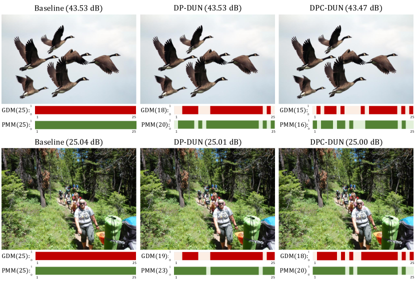
Figure 1: Two subjective examples of the impact of the active module number on the reconstruction performance (PSNR). We compare the “Baseline” model without the selectors and our models (DP-DUN and DPC-DUN) with the selectors when ratio $=30\%$. While maintaining similar high performance, our methods can adaptively select an appropriate path and an optimal number of active modules for different images.

Mathematically, a random linear measurement $\mathbf{y}\in\mathbb{R}^{M}$ can be formulated as $\mathbf{y}=\mathbf{\Phi}\mathbf{x}$, where $\mathbf{x}\in\mathbb{R}^{N}$ is the original signal and $\mathbf{\Phi}\in\mathbb{R}^{M\times N}$ is the measurement matrix with $M\ll N$. $\frac{M}{N}$ is the CS ratio (or sampling rate). Obviously, CS reconstruction is an ill-posed inverse problem. To obtain a reliable reconstruction, the conventional CS methods commonly solve an energy function as follows:

$$\begin{split}\underset{\mathbf{x}}{\arg\min}\leavevmode\nobreak\ \leavevmode\nobreak\ \frac{1}{2}\left\|\mathbf{\Phi}\mathbf{x}-\mathbf{y}\right\|^{2}_{2}+\lambda\mathcal{R}(\mathbf{x}),\end{split}$$ (1)

where $\frac{1}{2}\left\|\mathbf{\Phi}\mathbf{x}-\mathbf{y}\right\|^{2}_{2}$ denotes the data-fidelity term and $\lambda\mathcal{R}(\mathbf{x})$ denotes the prior term with regularization parameter $\lambda$. For traditional model-based methods [15, 16, 17, 18, 19, 20, 21], the prior term can be the sparsifying operator corresponding to some pre-defined transform basis, such as discrete cosine transform (DCT) and wavelet [22, 23]. They enjoy the merits of strong convergence and theoretical analysis in most cases but are usually limited in high computational complexity and challenges of tuning parameters [24].

Recently, fueled by the powerful learning capacity of deep networks, several network-based CS algorithms have been proposed [25, 26]. Apparently compared with model-based methods, they can represent image information flexibly with fast inferences, but the architectures of most network-based methods are empirically designed, and the achievements of traditional algorithms are not fully considered [27]. More recently, some deep unfolding networks (DUNs) with good interpretability have been proposed to combine network with optimization and train a truncated unfolding inference through an end-to-end learning manner, which has become the mainstream for CS [28, 29, 30, 31, 32].

DUN is usually composed of a fixed number of stages, where each stage corresponds to an iteration. Theoretically, increasing the unfolded iteration number will make the recovered results closer to the original images. However, do we need the whole network trunk to process indiscriminately all images containing different information? In reality, the content of different images is substantially different, and some images are inherently easier to restore than others. Two subjective examples are shown in Fig 1, and we try to analyze whether reducing the module numbers in the stages affects reconstruction performance. The stage numbers are all 25 in different models, and each stage contains a gradient descent module (GDM) and a proximal mapping module (PMM). We do experiments to skip some modules (masked as 0) and execute others (masked as 1) by using selectors on our proposed methods (DP-DUN/DPC-DUN), and count the number of the performed modules (dubbed active modules), from which we can see that adaptively selecting a proper path and an optimal number of active modules can maintain similar high performance while largely reducing the computational cost. This observation motivates the possibility of saving computations by selecting a different path for each image based on its content.

This paper proposes a dynamic path-controllable deep unfolding network (DPC-DUN) for image CS. In DPC-DUN, we design a path-controllable selector (PCS) that comprises a path selector (PS) and a controllable unit (CU), which dynamically adjusts the active module numbers at test time conditioned on the Lagrange multiplier. PS adaptively selects an appropriate path and changes the number and position of the active modules for images with different content. CU takes the Lagrange multiplier as the input and produces a latent representation to control the performance-complexity tradeoff. Our DPC-DUN is a comprehensive framework, considering the merits of previous optimization-inspired DUNs, adjusting the utilization of module numbers, and simplifying the processing pipeline. It enjoys the advantages of both the satisfaction of interpretability and scalability. The major contributions are summarized as follows:

• We propose a novel Dynamic Path-Controllable Deep Unfolding Network (DPC-DUN), which shows a slimming mechanism that adaptively selects different paths and enables model interactivity with controllable complexity.

• We introduce a Path Selector (PS) which utilizes the skip connection structure inherent in DUNs and adaptively determines the number and position of modules executed.

• We design a Path-Controllable Selector (PCS) which achieves dynamic adjustment with a controllable unit (CU) and gets a suitable performance-complexity tradeoff to meet the needs in practice.

• Extensive experiments show that DPC-DUN enables the control of different tradeoffs and achieves good performance.

The rest of the paper is organized as follows. Section II introduces related work. Then we propose our approach DPC-DUN in Section III. Section IV presents experimental results. Finally, Section V draws conclusions.

II Related work

II-A Deep Unfolding Network

Deep unfolding networks (DUNs) have been proposed to solve different image inverse tasks, such as denoising [33, 34], deblurring [35, 36], and demosaicking [37]. DUN has friendly interpretability on training data pairs $\{(\mathbf{y}_{j},\mathbf{x}_{j})\}_{j=1}^{N_{a}}$, which is usually formulated on CS construction as the bi-level optimization problem:

$$\begin{split}&\underset{\Theta}{\min}\sum_{j=1}^{N_{a}}{\mathcal{L}(\mathbf{\hat{x}}_{j},\mathbf{x}_{j})},\\ &\mathbf{s.t.}\ \mathbf{\hat{x}}_{j}=\underset{\mathbf{x}}{\arg\min}\frac{1}{2}\left\|\mathbf{\Phi}\mathbf{x}-\mathbf{y}_{j}\right\|^{2}_{2}+\lambda\mathcal{R}(\mathbf{x}).\end{split}$$ (2)

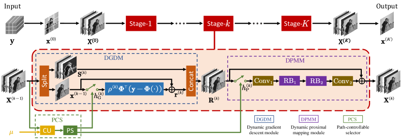
Figure 2: The architecture of our proposed DPC-DUN which consists of $K$ stages. $\mathbf{y}$ is the under-sampled data as the input of the model, $\mathbf{x}^{(0)}=\mathbf{\Phi^{\top}}\mathbf{y}$ denotes the initialization, $\mathbf{x}^{(K)}$ denotes the recovered result and $\mathbf{X}^{(k)}$ stands for the output features of the $k$-th unrolled stage. In addition to the main processing path marked in black, the green line controls whether the Dynamic Gradient Descent Module (DGDM) and the Dynamic Proximal Mapping Module (DPMM) are selected by the Path-Controllable Selector (PCS) which consists of the Controllable Unit (CU) and the Path Selector (PS), and the yellow line denotes the modulation process with the Lagrange multiplier $\mu$.

DUNs on CS usually integrate some effective convolutional neural network (CNN) denoisers into some optimization methods, including half quadratic splitting (HQS) algorithm [38, 39], proximal gradient descent (PGD) algorithm [28, 40, 31, 41, 42], and inertial proximal algorithm for nonconvex optimization (iPiano) [43]. Different optimization methods usually lead to different optimization-inspired DUNs. The structures of existing DUNs generally are elaborately designed under a fixed number of iterations and do not consider the effect of different stage numbers in a model, which causes processing of all images with a single path and makes these methods less efficient [44]. However, the solution has not yet been found to apply in DUNs which are a kind of model based on regularly iterative optimization algorithms.

II-B Dynamic Network

Dynamic networks [45] have been investigated to achieve a better tradeoff between complexity and performance in different tasks [46, 47, 48]. Yu et al. [44] propose the pathfinder which can dynamically select an appropriate network path to save the computational cost. And some approaches [49, 50] are proposed to skip some residual blocks with skip connection in ResNet [51] by using a gating network. These methods successfully explore routing policies and touch off the thinking of skip connection. The optimization algorithms applied in DUNs generally have inherent structures of skip connection. Therefore, DUNs have critical physical properties to adaptively achieve the goal of dynamic path selection and minimize the computation burden at the test time.

II-C Controllable Network

Many controllable networks interpolate the parameters to adjust restored effect for various degradation levels [52, 31, 53, 54], which inspire us to design an adjustable model that can be run at different performance-complexity tradeoff on CS reconstruction. Choi et al. [55] and Lin et al. [56] develop variable-rate learned image compression framework using the control parameters to modulate the internal feature maps in the autoencoder and propose highly flexible models that provide dynamic adjustment of computational cost, thus addressing the main requirements in practical image compression.

III Proposed Method

In this section, we will elaborate on the design of our proposed dynamic path-controllable deep unfolding network (DPC-DUN) for image CS.

III-A Framework

As widely recognized knowledge, DUN is generally a typical CNN-based method often constructed with an efficient iterative algorithm. The proximal gradient descent (PGD) algorithm is well-suited for solving many large-scale linear inverse problems. Traditional PGD solves the CS reconstruction problem in Eq. (1) by iterating between the following two update steps:

$$\mathbf{r}^{(k)}=\mathbf{x}^{(k-1)}-\rho^{(k)}\mathbf{\Phi^{\top}}\left(\mathbf{\Phi}\mathbf{x}^{(k-1)}-\mathbf{{y}}\right),$$ (3)

$$\mathbf{x}^{(k)}=\underset{\mathbf{x}}{\arg\min}\frac{1}{2}\left\|\mathbf{x}-\mathbf{r}^{(k)}\right\|^{2}_{2}+\lambda\mathcal{R}(\mathbf{x}),$$ (4)

where $k\in\{1,2,\cdots,K\}$ is the stage index, $\mathbf{x}^{(k)}$ is the output image of the $k$-th stage, $\mathbf{\Phi^{\top}}$ is the transpose of the measurement matrix $\mathbf{\Phi}\in\mathbb{R}^{M\times N}$ and $\rho^{(k)}$ is the learnable descent step size. $\mathbf{y}=\mathbf{\Phi\mathbf{x}}$ is the sampled image produced by an image $\mathbf{x}\in\mathbb{R}^{H\times W}$ which is divided into $\frac{H}{\sqrt{N}}\times\frac{W}{\sqrt{N}}$ non-overlapping image blocks with size of $\sqrt{N}\times\sqrt{N}$.

Eq. (3) is implemented by a gradient descent module (GDM) which is trivial [28] and Eq. (4) is achieved by a proximal mapping module (PMM) which is actually a CNN-based denoiser. Motivated that multi-channel feature transmission well ensures maximum signal flow [41], we improve PMM with high-throughput information and the iterative process in the $k$-th stage, as shown in Fig. 2 (indicated by the black line), can be formulated as:

$$\mathbf{R}^{(k)}=\mathcal{G}_{\operatorname{GDM}}(\mathbf{X}^{(k-1)}),$$ (5)

$$\mathbf{X}^{(k)}=\mathcal{G}_{\operatorname{PMM}}(\mathbf{R}^{(k)}),$$ (6)

where $\mathbf{R}^{(k)}$, $\mathbf{X}^{(k)}$ $\in\mathbb{R}^{C\times H\times W}$ are as the outputs of the $k$-th stage in feature domain. The initialization $\mathbf{X}^{(0)}$ is generated by concatenating the $\mathbf{x}^{(0)}$ and the feature maps ($\in\mathbb{R}^{(C-1)\times H\times W}$) applying a one-convolution layer on the $\mathbf{x}^{(0)}$.

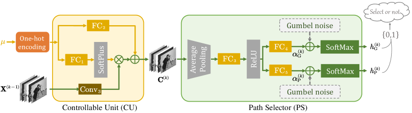
Figure 3: The architecture of our proposed Path-Controllable Selector (PCS) which consists of the controllable unit (CU) and the path selector (PS). The Gumbel noise in the path selector is only added to achieve end-to-end training.

To reduce the loss of information, we split the input $\mathbf{X}^{(k-1)}$ into two chunks, dubbed one-channel $\mathbf{x}^{(k-1)}$ which is as the input of Eq. (3), and $(C-1)$-channel $\mathbf{S}^{(k)}$ which is concatenated with the output of Eq. (3) along channel dimension. Therefore, the complete process of $\mathcal{G}_{\operatorname{GDM}}(\cdot)$ based on Eq. (3) is

$$\mathbf{x}^{(k-1)},\mathbf{S}^{(k)}=\operatorname{Split}\left(\mathbf{X}^{(k-1)}\right),$$ (7a)

$$\mathbf{r}^{(k)}=\rho^{(k)}\mathbf{\Phi^{\top}}\left(\mathbf{{y}}-\mathbf{\Phi}\mathbf{x}^{(k-1)}\right)+\mathbf{x}^{(k-1)},$$ (7b)

$$\mathbf{R}^{(k)}=\operatorname{Concat}\left(\mathbf{r}^{(k)},\mathbf{S}^{(k)}\right),$$ (7c)

where $\mathbf{x}^{(k-1)}=\mathbf{X}^{(k-1)}[0:1,:,:\ ],\mathbf{S}^{(k)}=\mathbf{X}^{(k-1)}[1:C,:,:\ ]$.

Therefore, GDM can be expressed by a formula:

$$\mathbf{R}^{(k)}=\operatorname{Concat}(\rho^{(k)}\mathbf{\Phi^{\top}}\left(\mathbf{{y}}-\mathbf{\Phi}\mathbf{x}^{(k-1)}\right)+\mathbf{x}^{(k-1)},\ \mathbf{S}^{(k)}).$$ (8)

PMM consists of two basic convolution layers ($\operatorname{Conv}_{1}$ and $\operatorname{Conv}_{2}$) and two residual blocks ($\operatorname{RB}_{1}$ and $\operatorname{RB}_{2}$), which keeps the high recovery accuracy with the simple structure [41]. The module $\mathcal{G}_{\operatorname{PMM}}(\cdot)$ is formulated as:

$$\mathbf{X}^{(k)}=\operatorname{Conv}_{2}(\operatorname{RB}_{2}(\operatorname{RB}_{1}(\operatorname{Conv}_{1}(\mathbf{R}^{(k)}))))+\mathbf{R}^{(k)}.$$ (9)

In DUNs, the stage number $K$ is generally fixed and cannot adaptively adjust based on the input image, which consumes much memory and unnecessary computational cost. Moreover, according to the different needs of users, developing controllable models that can flexibly handle the efficiency-accuracy tradeoff is essential and practical. Therefore, we design a Path-Controllable Selector (PCS) applying in GDM and PMM and propose a dynamic gradient descent module (DGDM) and a dynamic proximal mapping module (DPMM).

III-B Path-Controllable Selector (PCS)

As shown in Fig. 3, the path-controllable selector (PCS) consists of two parts: a controllable unit and a path selector. The Path Selector (PS) can dynamically select an optimal path for each image with different content, and the Controllable Unit (CU) can enable control of computation and memory while combining with the PS. In the following, we will introduce the PS and the CU, respectively.

III-B1 Path Selector (PS)

The motivation of the path selector (PS) aims at predicting a one-hot vector, which denotes whether to execute or skip the module (i.e., the decision is to skip the module when PS predicts 0.). Since a non-differentiable problem exists in the process from the continuous feature outputs to discrete path selection, we adopt the Gumbel Softmax trick [57, 46, 58] to make the discrete decision differentiable during the back-propagation.

To meet our needs, we first choose two resolution candidates $\alpha^{(k)}_{1}$ and $\alpha^{(k)}_{2}$ at the $k$-th stage to shrink the exploration range. $\alpha^{(k)}=[\alpha^{(k)}_{1},\alpha^{(k)}_{2}]\in\mathbb{R}^{2}$ is the output signal that represents the probability of each candidate. Then, we apply Gumbel Softmax trick to turn soft decisions $\alpha^{(k)}$ into hard decisions $h^{(k)}=[h^{(k)}_{1},h^{(k)}_{2}]$, and the expression can be written as:

$$h^{(k)}_{i}=\frac{\exp{(\alpha^{(k)}_{i}+n^{(k)}_{i}/\tau)}}{\sum_{i=1}^{2}\exp{(\alpha^{(k)}_{i}+n^{(k)}_{i}/\tau)}},$$ (10)

where $h^{(k)}_{i}\in\{0,1\}$. $n^{(k)}_{i}\sim\operatorname{Gumbel}(0,1)$ is a random noise sampled from the Gumbel distribution, which is only adopted in the training phase. $\tau$ is a temperature parameter to influence the Gumbel Softmax function and set it as 1.

Inspired by squeeze-and-excitation (SE) network [59], we design two PSs (${h}^{(k)}_{\text{G}}$ and ${h}^{(k)}_{\text{P}}$) with the same structure to control GDM and PMM respectively, as shown in Fig. 3. The selectors ${h}^{(k)}_{\text{G}}=\mathcal{H}_{\operatorname{G}}(\mathbf{C^{(k)}})$ and ${h}^{(k)}_{\text{P}}=\mathcal{H}_{\operatorname{P}}(\mathbf{C^{(k)}})$ are formulated as:

$${h}^{(k)}_{\text{G}}=\operatorname{GS}(\operatorname{FC}^{(k)}_{4}(\operatorname{ReLU}(\operatorname{FC}^{(k)}_{3}(\operatorname{AveragePool}(\mathbf{C}^{(k)}))))),$$ (11)

$${h}^{(k)}_{\text{P}}=\operatorname{GS}(\operatorname{FC}^{(k)}_{5}(\operatorname{ReLU}(\operatorname{FC}^{(k)}_{3}(\operatorname{AveragePool}(\mathbf{C}^{(k)}))))).$$ (12)

The input feature $\mathbf{C^{(k)}}$ is firstly squeezed by an average pooling operation in each channel to produce the $C$-channel feature maps. Then we reduce the feature dimensions by 4 in the fully-connected layer $\operatorname{FC^{(k)}_{3}}(\cdot)$. The non-linear activation function ($\operatorname{ReLU}(\cdot)$) and the fully-connected layer ($\operatorname{FC^{(k)}_{4}}(\cdot)$ or $\operatorname{FC^{(k)}_{5}}(\cdot)$) are further leveraged to generate the resolution candidate $\alpha^{(k)}_{\text{G}}$ or $\alpha^{(k)}_{\text{P}}$. Finally, the one-hot selections ${h}^{(k)}_{\text{G}}=[{h}^{(k)}_{\text{G1}},{h}^{(k)}_{\text{G2}}]\in\{0,1\}^{2},\ {h}^{(k)}_{\text{P}}=[{h}^{(k)}_{\text{P1}},{h}^{(k)}_{\text{P2}}]\in\{0,1\}^{2}$ are obtained by the Gumbel Softmax function $(\operatorname{GS}(\cdot))$.

Eq. (7b) and Eq. (9) that both use the residual connection are the primary sources of computation requirement in the main process. Inspired by the controllable residual connection in CResMD [52], we add the two PSs to control the summation weight, respectively. Therefore, the network adding the dynamical PSs, dubbed DP-DUN, is iterated by following two update steps:

$$\begin{split}\mathbf{R}^{(k)}=&\operatorname{Concat}(h^{(k)}_{\text{G1}}\cdot\rho^{(k)}\mathbf{\Phi^{\top}}\left(\mathbf{{y}}-\mathbf{\Phi}\mathbf{x}^{(k-1)}\right)+h^{(k)}_{\text{G2}}\cdot\mathbf{x}^{(k-1)},\mathbf{S}^{(k)}),\\ \mathbf{X}^{(k)}=&\ h^{(k)}_{\text{P1}}\cdot\operatorname{Conv}_{2}(\operatorname{RB}_{2}(\operatorname{RB}_{1}(\operatorname{Conv}_{1}(\mathbf{R}^{(k)}))))+h^{(k)}_{\text{P2}}\cdot\mathbf{R}^{(k)}.\end{split}$$ (13)

$$\begin{split}\mathbf{R}^{(k)}=&\operatorname{Concat}(h^{(k)}_{\text{G}}\cdot\rho^{(k)}\mathbf{\Phi^{\top}}\left(\mathbf{{y}}-\mathbf{\Phi}\mathbf{x}^{(k-1)}\right)+\mathbf{x}^{(k-1)},\mathbf{S}^{(k)}),\\ \mathbf{X}^{(k)}=&\ h^{(k)}_{\text{P}}\cdot\operatorname{Conv}_{2}(\operatorname{RB}_{2}(\operatorname{RB}_{1}(\operatorname{Conv}_{1}(\mathbf{R}^{(k)}))))+\mathbf{R}^{(k)}.\end{split}$$ (14)

Thus, the residual parts can be skipped by setting $\{{h}^{(k)}_{\text{G1}}=0,\ {h}^{(k)}_{\text{G2}}=1\}$ or $\{{h}^{(k)}_{\text{P1}}=0,\ {h}^{(k)}_{\text{P2}}=1\}$ and instead, they are performed.

In real-world scenarios, physical devices often impose different computing resource constraints on the model. Thus, the network should be developed considering various computational expenses. However, if we use the reconstruction loss only, the selector will tend to provide a sub-optimal solution [46], which conducts as many GDMs and PMMs as possible because features with the most enriched spatial information correspond to relatively higher reconstruction accuracy. To achieve a satisfactory efficiency-accuracy tradeoff, we propose a new selection loss $\mathcal{L}_{select}$ to guide the training. The loss $\mathcal{L}_{select}$ is designed by calculating the mean of the two PSs to obtain the selector prediction as:

$$\small\mathcal{L}_{select}=\ \frac{1}{K}\sum_{k=1}^{K}(h^{(k)}_{\text{G}}+h^{(k)}_{\text{P}}),$$ (15)

where $K$ represents the stage number. Therefore, the total loss function based on the reconstruction loss function $\mathcal{L}_{rec}$ can be optimized as follows:

$$\mathcal{L}=\mathcal{L}_{rec}+\mu\mathcal{L}_{select},$$ (16)

where the scalar factor $\mu>0$ in the Lagrangian is called a Lagrange multiplier to balance the accuracy expectation and computational cost constraints. As seen from the experimental results in Section IV-E , the value of $\mu$ decides different efficiency-accuracy tradeoffs, which is challenging to address the requirements in practice precisely. Therefore, we design a controllable unit (CU) to control the PS and propose DPC-DUN, which alternates between training the model and adjusting the different $\mu$ by introducing $\mu$.

III-B2 Controllable Unit (CU)

In Fig. 3, the Lagrange multiplier $\mu$ is firstly encoded as one-hot vector and then inputs two functions to get a parameter pair $(\mathbf{Q}^{(k)}(\mu),\mathbf{P}^{(k)}(\mu))$, which can be expressed as:

$$\mathbf{Q}^{(k)}(\mu)=\operatorname{Softplus}(\operatorname{FC}_{1}(\operatorname{onehot}(\mu))),$$ (17)

$$\mathbf{P}^{(k)}(\mu)=\operatorname{FC}_{2}(\operatorname{onehot}(\mu)),$$ (18)

where $\operatorname{FC}_{1}(\cdot)$ and $\operatorname{FC}_{2}(\cdot)$ are the fully-connected layers, $\operatorname{Softplus}(x)=\log(1+\exp(x))$. After obtaining the pair, we use the affine transformation to scale and shift the element-wise feature maps, which is shown as:

$$\mathbf{C}^{(k)}=\mathbf{Q}^{(k)}(\mu)\otimes\operatorname{Conv}_{3}(\mathbf{X}^{(k-1)})+\mathbf{P}^{(k)}(\mu),$$ (19)

The controllable unit, denoted by $\mathbf{C}^{(k)}=\mathcal{H}_{\operatorname{CU}}(\mathbf{X}^{(k-1)},\mu)$, is expressed as:

$$\begin{split}\mathbf{C}^{(k)}=&\operatorname{Softplus}(\operatorname{FC}_{1}(\operatorname{onehot}(\mu)))\otimes\operatorname{Conv}_{3}(\mathbf{X}^{(k-1)})\\ &+\operatorname{FC}_{2}(\operatorname{onehot}(\mu)).\end{split}$$ (20)

Hence, our proposed path-controllable selectors (PCSs) consisting of the controllable unit (CU) and the path selector (PS) can be formulated as:

$$\begin{split}&{h}^{(k)}_{\text{G}}(\mu)=\mathcal{H}_{\operatorname{G}}(\mathcal{H}_{\operatorname{CU}}(\mathbf{X}^{(k-1)},\mu)),\\ &{h}^{(k)}_{\text{P}}(\mu)=\mathcal{H}_{\operatorname{P}}(\mathcal{H}_{\operatorname{CU}}(\mathbf{X}^{(k-1)},\mu)).\end{split}$$ (21)

Our proposed Dynamic Path-Controllable Deep Unfolding Network (DPC-DUN) solves the CS reconstruction problem by iterating the dynamic gradient descent module (DGDM) and the dynamic proximal mapping module (DPMM) which are both adding PCS based on GDM and PMM respectively. According, $\mathbf{R}^{(k)}=\mathcal{G}_{\operatorname{DGDM}}(\mathbf{X}^{(k-1)},\mu)$ and $\mathbf{X}^{(k)}=\mathcal{G}_{\operatorname{DPMM}}(\mathbf{R}^{(k)},\mu)$ can be expressed as:

$$\begin{split}\mathbf{R}^{(k)}=&\operatorname{Concat}(h^{(k)}_{\text{G1}}(\mu)\cdot\rho^{(k)}\mathbf{\Phi^{\top}}\left(\mathbf{{y}}-\mathbf{\Phi}\mathbf{x}^{(k-1)}\right)+h^{(k)}_{\text{G2}}(\mu)\cdot\mathbf{x}^{(k-1)},\\ &\mathbf{S}^{(k)}),\\ \mathbf{X}^{(k)}=&\ h^{(k)}_{\text{P1}}(\mu)\cdot\operatorname{Conv}_{2}(\operatorname{RB}_{2}(\operatorname{RB}_{1}(\operatorname{Conv}_{1}(\mathbf{R}^{(k)}))))+h^{(k)}_{\text{P2}}(\mu)\cdot\mathbf{R}^{(k)}.\end{split}$$ (22)

III-C Loss function

The reconstruction loss $\mathcal{L}_{rec}$ in this work is the $L_{1}$ loss function, denoted by

$$\mathcal{L}_{rec}(\mu)=\ \frac{1}{{N}{N_{a}}}\sum_{j=1}^{N_{a}}{\left\|\mathbf{x}_{j}-\mathbf{x}_{j}^{(K)}(\mu)\right\|}_{1},$$ (23)

where $N_{a}$ represents the number of training images, $N$ represents the size of each image, $\left\{\mathbf{x}_{j}\right\}_{j=1}^{N_{a}}$ is a set of full-sampled images and $\left\{\mathbf{x}_{j}^{(K)}(\mu)\right\}_{j=1}^{N_{a}}$ is the corresponding reconstruction result with the controlling coefficient $\mu$.

Based on Eq. (15), the selection loss function is updated to be

$$\mathcal{L}_{select}(\mu)=\ \frac{1}{K}\sum_{k=1}^{K}(h^{(k)}_{\text{G}}(\mu)+h^{(k)}_{\text{P}}(\mu)).$$ (24)

Therefore, the total loss function can be expressed as below:

$$\mathcal{L}(\mu)=\mathcal{L}_{rec}(\mu)+\mu\mathcal{L}_{select}(\mu).$$ (25)

IV Experiments

IV-A Implementation Details

Table I: Average PSNR(dB)/SSIM performance comparisons on Set11 dataset [25] with different CS ratios. We compare our methods with nine competing methods. The best and second best PSNR/SSIM results are highlighted in red and blue colors, respectively. The number of GDM/PMM executed is highlighted in cyan.

CS Ratio	10%		25%		30%		40%		50%
	PSNR	SSIM	PSNR	SSIM	PSNR	SSIM	PSNR	SSIM	PSNR	SSIM
IRCNN [38]	23.05	0.6789	28.42	0.8382	29.55	0.8606	31.30	0.8898	32.59	0.9075
ReconNet [25]	23.96	0.7172	26.38	0.7883	28.20	0.8424	30.02	0.8837	30.62	0.8983
GDN [40]	23.90	0.6927	29.20	0.8600	30.26	0.8833	32.31	0.9137	33.31	0.9285
DPDNN [39]	26.23	0.7992	31.71	0.9153	33.16	0.9338	35.29	0.9534	37.63	0.9693
ISTA-Net+ [28]	26.58	0.8066	32.48	0.9242	33.81	0.9393	36.04	0.9581	38.06	0.9706
DPA-Net [26]	27.66	0.8530	32.38	0.9311	33.35	0.9425	35.21	0.9580	36.80	0.9685
MAC-Net [42]	27.68	0.8182	32.91	0.9244	33.96	0.9372	35.94	0.9560	37.67	0.9668
iPiano-Net [43]	28.33	0.8548	33.60	0.9368	34.90	0.9487	37.02	0.9638	38.85	0.9736
COAST [31]	28.74	0.8619	33.98	0.9407	35.11	0.9505	37.11	0.9646	38.94	0.9744
DP-DUN	29.42	0.8806	34.75	0.9483	36.02	0.9577	38.06	0.9698	39.90	0.9791
	(22.9/23.2)		(19.0/20.7)		(21.0/22.9)		(19.0/21.4)		(17.0/20.9)
DPC-DUN	29.40	0.8798	34.69	0.9482	35.88	0.9570	37.98	0.9694	39.84	0.9778
	(20.5/21.6)		(17.8/18.9)		(16.5/18.3)		(16.5/18.6)		(14.6/17.5)

Table II: Average PSNR(dB)/SSIM performance comparisons on CBSD68 dataset [60] with different CS ratios. We compare our methods with nine competing methods. The best and second best PSNR/SSIM results are highlighted in red and blue colors, respectively. The number of GDM/PMM executed is highlighted in cyan.

CS Ratio	10%		25%		30%		40%		50%
	PSNR	SSIM	PSNR	SSIM	PSNR	SSIM	PSNR	SSIM	PSNR	SSIM
IRCNN [38]	23.07	0.5580	26.44	0.7206	27.31	0.7543	28.76	0.8042	30.00	0.8398
ReconNet [25]	24.02	0.6414	26.01	0.7498	27.20	0.7909	28.71	0.8409	29.32	0.8642
GDN [40]	23.41	0.6011	27.11	0.7636	27.52	0.7745	30.14	0.8649	30.88	0.8763
DPDNN [39]	25.35	0.7020	29.28	0.8513	30.39	0.8807	32.21	0.9171	34.27	0.9455
ISTA-Net+ [28]	25.37	0.7022	29.32	0.8515	30.37	0.8786	32.23	0.9165	34.04	0.9425
DPA-Net [26]	25.47	0.7365	29.01	0.8589	29.73	0.8821	31.17	0.9151	32.55	0.9382
MAC-Net [42]	25.80	0.7018	29.42	0.8464	30.28	0.8707	32.02	0.9074	33.68	0.9348
iPiano-Net [43]	26.34	0.7431	30.16	0.8711	31.24	0.8964	33.14	0.9298	34.98	0.9521
COAST [31]	26.43	0.7450	30.24	0.8724	31.20	0.8947	33.03	0.9273	34.81	0.9497
DP-DUN	26.82	0.7601	30.76	0.8837	31.83	0.9059	33.77	0.9369	35.72	0.9581
	(23.0/23.4)		(19.0/21.0)		(21.0/22.7)		(18.8/21.1)		(17.0/20.2)
DPC-DUN	26.79	0.7611	30.71	0.8828	31.76	0.9051	33.70	0.9364	35.62	0.9573
	(19.6/21.6)		(17.7/19.4)		(17.2/18.5)		(16.2/18.0)		(14.3/16.9)

Table III: Average PSNR(dB)/SSIM performance comparisons on Urban100 [39] and DIV2K [61] datasets with different CS ratios. We compare our methods with three competing methods. The best and second best results are highlighted in red and blue colors, respectively. The numbers of GDM/PMM executed are highlighted in cyan.

Dataset	Methods	CS Ratio
		5%	10%	25%	30%	40%	50%
Urban100	ISTA-Net+ [28]	20.70/0.5886	23.61/0.7238	28.93/0.8840	30.21/0.9079	32.43/0.9377	34.43/0.9571
	iPiano-Net [43]	22.48/0.6728	25.67/0.7963	30.87/0.9157	32.16/0.9320	34.27/0.9531	36.22/0.9675
	COAST [31]	22.45/0.6800	25.94/0.8035	31.10/0.9168	32.23/0.9321	34.22/0.9530	35.99/0.9665
	DP-DUN	23.61/0.7268	27.03/0.8335	32.43/0.9328	33.70/0.9464	35.69/0.9628	37.63/0.9743
		(23.0/25.0)	(22.9/23.3)	(19.0/21.1)	(21.0/22.8)	(18.9/21.9)	(17.0/21.2)
	DPC-DUN	23.43/0.7177	26.99/0.8345	32.36/0.9323	33.53/0.9449	35.61/0.9624	37.52/0.9737
		(16.0/17.4)	(20.5/21.7)	(18.2/19.5)	(17.3/18.5)	(16.3/18.3)	(14.7/17.5)
DIV2K	ISTA-Net+ [28]	25.15/0.6922	27.73/0.7859	32.24/0.9007	33.43/0.9201	35.43/0.9450	37.33/0.9617
	iPiano-Net [43]	26.38/0.7410	28.94/0.8232	33.29/0.9164	34.47/0.9326	36.50/0.9539	38.36/0.9677
	COAST [31]	26.37/0.7464	29.17/0.8276	33.45/0.9178	34.49/0.9323	36.41/0.9530	38.22/0.9668
	DP-DUN	27.07/0.7630	29.70/0.8401	34.13/0.9257	35.29/0.9403	37.27/0.9591	39.11/0.9711
		(23.0/25.0)	(23.0/23.3)	(19.0/20.7)	(21.0/22.4)	(18.7/21.1)	(17.0/20.2)
	DPC-DUN	26.98/0.7626	29.67/0.8423	34.08/0.9257	35.20/0.9397	37.20/0.9588	39.11/0.9713
		(15.8/17.5)	(19.4/21.2)	(17.5/18.8)	(16.4/18.0)	(15.4/17.5)	(14.1/16.7)

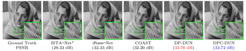
Figure 4: Comparisons on recovering an image (“Barbara”) from Set11 dataset [25] in the case of CS ratio = 25$\%$.

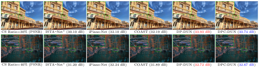
Figure 5: Comparisons on an image from Urban100 dataset [39] in the case of CS ratio = 30% (upper) and an image from DIV2K dataset [61] in the case of CS ratio = 40% (lower).

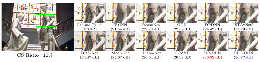
Figure 6: Comparisons on recovering an image from CBSD68 dataset [60] in the case of CS ratio = 10%.

Table IV: The computation cost and parameter number comparisons of all modules.

	GDM	PMM	CU	PS
FLOPs	$9.1\times 10^{7}$	$7.7\times 10^{9}$	$1.3\times 10^{9}$	$5.6\times 10^{2}$
Paras	1	55424	11296	292

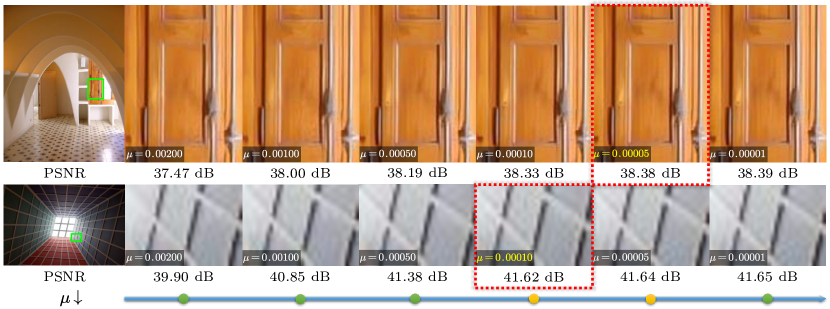
Figure 7: Illustration of recovering two images from Urban100 dataset [39] when CS ratio = $10\%$ under different $\mu$ with one single DPC-DUN model. The recovery accuracies and computational costs stably increase and converge with a gradual reduction of $\mu$. Users in various scenarios can adjust the suppression intensity on resource burden by a sliding bar (in blue) to find satisfactory tradeoffs with higher accuracy and lower cost, and the ideal settings are marked in red boxes with yellow setting color.

Table V: Average PSNR(dB)/FLOPs($10^{9}$)/$N_{AM}$ performance comparisons on Set11 [25] and CBSD68 [60] datasets with different stage number when CS ratio is $30\%$. After using the PS or PCS, the PSNR value remains unchanged, and the computation FLOPs drops more obviously with the larger number of stages.

Stage Number		Set11				CBSD68
		20	25	30	35	20	25	30	35
w/o PS	PSNR(dB)	35.98	36.05	36.07	36.10	31.81	31.85	31.86	31.87
	FLOPs($10^{9}$)	155.9	193.6	232.2	271.0	363.0	453.7	544.4	635.1
w/ PS	PSNR(dB)	35.99	36.02	36.06	36.08	31.82	31.83	31.84	31.86
	FLOPs($10^{9}$)	154.9	178.2	186.1	238.9	361.0	414.0	433.2	552.9
	$N_{AM}$	18.0/19.9	21.0/22.9	22.0/23.9	26.1/30.7	18.0/19.8	21.0/22.7	22.0/23.8	26.0/30.3
w/ PCS	PSNR(dB)	35.89	35.88	35.93	35.98	31.76	31.76	31.79	31.79
	FLOPs($10^{9}$)	167.8	174.5	182.2	206.2	389.4	412.8	460.5	490.5
	$N_{AM}$	16.0/18.3	16.5/18.3	17.5/19.5	18.1/20.7	15.6/18.1	17.2/18.5	17.7/20.3	17.9/21.1

Table VI: The Memory/FLOPs/PSNR performance on Set11 dataset.

Method	iPiano-Net	COAST	DP-DUN	DPC-DUN
Mem.(MB)	1810	1544	1312	1442
FLOPs($10^{9}$)	1426.7	157.7	72.0	138.0
PSNR(dB)	34.78	35.11	35.34	35.54

We use the 400 training images of size $180\times 180$ [33], generating the training data pairs $\{(\mathbf{y}_{j},\mathbf{x}_{j})\}_{j=1}^{N_{a}}$ by extracting the luminance component of each image block of size $33\times 33$, i.e. $N=1,089$. Meanwhile, we apply the data augmentation technique to increase the data diversity. For a given CS ratio, the corresponding measurement matrix $\mathbf{\Phi}\in\mathbb{R}^{M\times N}$ is constructed by generating a random Gaussian matrix and then orthogonalizing its rows, i.e. $\mathbf{\Phi}\mathbf{\Phi^{\top}}=\mathbf{I}$, where $\mathbf{I}$ is the identity matrix. The sampling process applies a convolution layer whose kernel is the matrix $\mathbf{\Phi}$. Applying $\mathbf{y}_{j}=\mathbf{\Phi}\mathbf{x}_{j}$ yields the set of CS measurements, where $\mathbf{x}_{j}$ is the vectorized version of an image block and is initialized by $\mathbf{x}_{j}^{(0)}=\mathbf{\Phi^{\top}}\mathbf{y}_{j}$.

Our proposed models are trained with 410 epochs separately for each CS ratio. Each image block of size $33\times 33$ is sampled and reconstructed independently for the first 400 epochs, and for the last ten epochs, we adopt larger image blocks of size $99\times 99$ as the inputs to finetune the model further. To alleviate blocking artifacts, we firstly unfold the blocks of size $99\times 99$ into overlapping blocks of size $33\times 33$ while sampling process $\mathbf{\Phi}\mathbf{x}$ and then fold the blocks of size $33\times 33$ into larger blocks while initialization $\mathbf{\Phi^{\top}}\mathbf{y}$ [43]. We also unfold the whole image with this approach during testing. We use momentum of 0.9 and weight decay of 0.999. The default batch size is 64, the default stage number $K$ is 25, the default number of feature maps $C$ is 32, and the learnable parameter $\rho^{(k)}$ is initialized to 1. In the training phase, the default Lagrange multiplier $\mu$ is randomly chosen as the input of DPC-DUN from the range of $\{0.00001,0.00005,0.0001,0.0005,0.001,0.002\}$. The CS reconstruction accuracies on all datasets are evaluated with PSNR and SSIM. And we also show the active module number ($N_{AM}$) and the computation cost (including the computations of the convolution and the fully-connected layer) measured in floating-point operations per second (FLOPs).

IV-B Qualitative Evaluation

We compare our proposed DP-DUN ($\mu=0.00005$) and DPC-DUN ($\mu=0.00001$) with some recent representative CS reconstruction methods. The average PSNR/SSIM reconstruction performances on Set11 [25] and CBSD68 [60] datasets with respect to five CS ratios are summarized in Table I and Table II respectively. Furthermore, Table III shows the comparisons with respect to six CS ratios on Urban100 [39] and DIV2K [61] datasets which contain more and larger images. One can observe that our DP-DUN and DPC-DUN outperform all the other competing methods in PSNR across all the cases. Compared with SCS-GNet [62], our methods achieve a high PSNR and slightly lower SSIM for some ratios in Table I. However, SCS-GNet takes more than half an hour to reconstruct an image of size 256 $\times$ 256 for testing, while our methods achieve real-time performance. So our methods can save resources while maintaining high performance. Therefore, our model applies well to the fixed Gaussian matrix and can be easily extended to other deterministic measurement matrices. In addition, the number of active modules decreases significantly, especially when the CS ratio is larger, and DPC-DUN can utilize the smaller numbers of GDM and PMM than DP-DUN in a less volatile range of the PSNR value. Fig. 4, Fig. 5, and Fig. 6 further show the visual comparisons of challenging images on various datasets. Our DP-DUN and DPC-DUN generate visually pleasant images that are faithful to the ground truth.

IV-C Cost Comparison

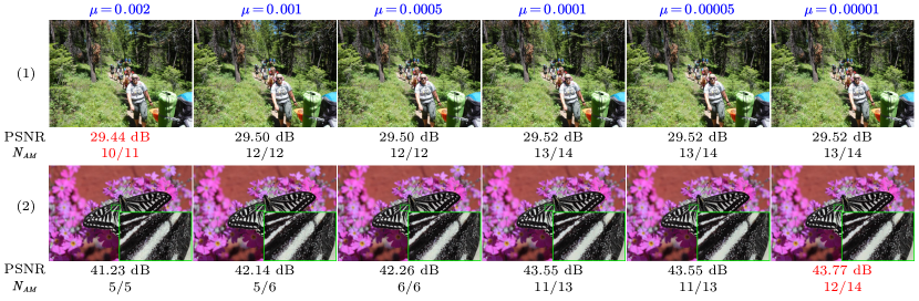
Figure 8: Illustration of recovering two images from DIV2K dataset [61] when CS ratio = $50\%$ under different $\mu$ with one single DPC-DUN model. The PSNR value and the active module numbers ($N_{AM}$) of GDM/PMM highlighted in red represent the optimal choice.

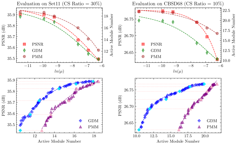
Figure 9: Visualization of the relationships among the factor $\mu$, the active module numbers of GDM/PMM, and PSNR on Set11 dataset [25] with CS ratio = 30$\%$ (left) and CBSD68 dataset [60] with CS ratio = 10% (right). The upper row shows the stable accuracy and computational cost reductions with the increase of $\mu$, and their inconsistent changing degrees under different settings. The lower row exhibits the scalability and robustness of DPC-DUN, which can flexibly generalize to unseen configurations by learning with only six default settings (highlighted in light colors with orange dotted lines).

We analyze the FLOPs on Set11 dataset and the parameter numbers of each module in Table IV. Compared with others, the lightweight path selector (PS) requires less storage space and computational overhead, which can help reduce the memory and cost of the network. What is more, Table V compares w/o PS, w/ PS and w/ PCS with different stage numbers when CS ratio is $30\%$. It is clear that the PSNR value remains unchanged when stage number $K\geqslant 25$, and although adding PS increases the computation costs of PS, the numbers of total FLOPs are reduced, especially when the stage number is much larger. Path-controllable selector (PCS), which contains PS and CU, gives the network less computational overhead than only using PS while the performance changes little, especially $K\geqslant 25$. Therefore, CU containing a convolution layer has more parameters but can reduce total model numbers compared with the non-adjustable model.

The GPU memory and FLOPs of some competing methods are provided in Table VI. Obviously, our DP-DUN/DPC-DUN ($\mu=0.002$) has less memory and computation cost than others while ensuring the best performance. This demonstrates that our methods can achieve the best performance-consumption balance by adjusting the multiplier.

IV-D Analysis of Path-Controllable Selector (PCS)

Table VII: Average performance comparisons on Set11 [25] and CBSD68 [60] datasets with various Lagrange multipliers when CS ratio is 30$\%$. The larger the value of $\mu$, the smaller the value of PSNR, the smaller the value of $N_{AM}$, and the lower the computation cost (FLOPs).

$\mu$		0	0.00001	0.00005	0.0001	0.0002	0.0005	0.001	0.002
Set11	PSNR(dB)	36.05	36.04	36.02	36.04	35.98	35.84	35.69	35.34
	FLOPs($10^{9}$)	194.0	185.9	178.2	182.0	157.9	116.6	98.7	72.4
	$N_{AM}$	25.0/24.9	21.0/23.9	21.0/22.9	21.0/23.4	17.5/20.3	12.4/15.0	9.6/12.7	8.2/9.3
CBSD68	PSNR(dB)	31.84	31.83	31.83	31.83	31.81	31.73	31.62	31.38
	FLOPs($10^{9}$)	452.8	430.3	414.0	426.6	368.1	284.1	220.3	164.1
	$N_{AM}$	25.0/24.8	21.0/23.6	21.0/22.7	20.9/23.4	17.1/20.2	12.0/15.6	9.0/12.1	7.6/9.0

By combining the information of a one-hot vector encoded by the Lagrange multiplier $\mu$ and the input image feature, DPC-DUN can dynamically balance the recovery accuracy and resource overhead with our proposed controllable mechanism achieved by PCS. In practice, users can interactively adjust the tradeoff of performance-complexity by manipulating a sliding bar, and find property values for specific scenarios. Fig. 7 presents our recoveries under different $\mu$ values and exhibits the customized reconstructions of DPC-DUN with stable performance. To more fully show the role of the modulation mechanism for the specific images, we present more qualitative results from DIV2K dataset [61] under different $\mu$ in Fig. 8. We find that with the increase of the $\mu$ value, the PSNR value increases insignificantly, and yet the number of the active module ($N_{AM}$) increases obviously in Fig. 8(1), so $\mu=0.002$ is the best choice to achieve the performance-complexity tradeoff for the easier image. For the image of Fig. 8(2) which contains rich contents, the performance and the computational complexity are influenced significantly by the value of $\mu$, and we select the setting $\mu=0.00001$ to maintain great reconstruction accuracy. Therefore, our DPC-DUN is designed more finely and specifically by controlling the value of $\mu$.

To analyze the relationships among $\mu$, active module numbers of GDM/PMM and PSNR, Fig. 9 shows the changes through evaluations on Set11 [25] and CBSD68 [60] datasets. From the upper subplot, we can see that PSNR and active module numbers generally keep consistent trends but maybe with different changing degrees under various sampling rates and data distributions. Moreover, to break the limits of the fixed one-hot vectors encoded by the modulation factor $\mu$, we explore the effect of other (unseen) binary encodings in our proposed method, as shown in the lower row of Fig. 9. In addition to the provided six default settings adopted in training, DPC-DUN can generalize to unseen encodings, enabling fine-granular model scalability. These facts verify our controllable and adaptive design’s good interactivity and high flexibility.

Table VIII: Average PSNR(dB)/SSIM/$N_{AM}$ performance results of DP-DUN/DPC-DUN on Set11 dataset, where “-” represents the results without fine-tuning (deblocking).

CS Ratio	10		30
	PSNR/SSIM	$N_{AM}$	PSNR/SSIM	$N_{AM}$
DP-DUN-	29.20/0.8737	23.0/23.0	35.93/0.9569	21.0/22.8
DP-DUN	29.42/0.8806	22.9/23.2	36.02/0.9577	21.0/22.9
DPC-DUN-	29.17/0.8740	20.3/21.4	35.69/0.9560	15.7/16.9
DPC-DUN	29.40/0.8798	20.5/21.6	35.88/0.9570	16.5/18.3

Table IX: Average PSNR(dB)/SSIM performance comparisons on Set11 dataset with learnable sampling matrix. The best performance is labeled in bold.

CS Ratio	10		30
	PSNR	SSIM	PSNR	SSIM
MADUN [41]	29.91	0.8986	36.94	0.9676
HQSRED-Net [63]	29.04	0.8678	35.58	0.9553
SCS-GNet [62]	29.35	0.8854	35.42	0.9588
TransCS [64]	29.54	0.8877	35.62	0.9588
DPC-DUN	30.00	0.9002	37.02	0.9677
	(13.0/24.0)		(12.9/23.5)

IV-E Analysis of Path Selector (PS)

In our proposed methods, path selector (PS) plays a significant role in minimizing the computation burden at test time, which is important for optimizing models to meet practical application needs. Lagrange multiplier $\mu$ in Eq. (16) represents the factor that selects a specific performance-complexity tradeoff point. We conduct experiments on Set11 [25] and CBSD68 [60] datasets to analyze the impact of different values of $\mu$ on different tradeoff, as shown in Table VII. The greater the value of $\mu$, the greater the weight of the model computation cost in the optimization problem, thus, the PSNR value is smaller, $N_{AM}$ and FLOPs are also smaller. Also, the PSNR value does not change obviously when $\mu\leqslant 0.0002$ and compared with $\mu=0$, the FLOPs on $\mu=0.0002$ is reduced about $18.2\%$ on Set11 dataset and about $18.6\%$ on CBSD68 dataset, which shows that adjusting PS can save computing resources extremely well.

IV-F Ablation Study

Table X: Comparisons of the robustness to Gaussian noise among different methods on Set11 dataset in the case of ratio = 10$\%$, where ^∗ represents the model is finetuned with mixed noises. And the difference of PSNR between w/o noise ($\sigma=0$) and w/ noise is highlighted in blue color.

Noise	ISTA-Net+[28]	ISTA-Net+∗	iPiano-Net[43]	iPiano-Net∗	DP-DUN	DP-DUN∗	DPC-DUN	DPC-DUN∗
$\sigma=0$	26.58( 0.00)	26.55( 0.00)	28.33( 0.00)	28.15( 0.00)	29.42( 0.00)	29.23( 0.00)	29.40( 0.00)	29.15( 0.00)
$\sigma=5$	25.92($\downarrow$0.66)	26.06($\downarrow$0.49)	27.56($\downarrow$0.77)	27.56($\downarrow$0.59)	28.33($\downarrow$1.09)	28.34($\downarrow$0.89)	28.26($\downarrow$1.14)	28.28($\downarrow$0.87)
$\sigma=7$	25.43($\downarrow$1.15)	25.70($\downarrow$0.85)	27.01($\downarrow$1.32)	27.15($\downarrow$1.00)	27.60($\downarrow$1.82)	27.80($\downarrow$1.43)	27.58($\downarrow$1.82)	27.76($\downarrow$1.39)
$\sigma=10$	24.61($\downarrow$1.97)	25.04($\downarrow$1.51)	26.14($\downarrow$2.19)	26.33($\downarrow$1.82)	26.60($\downarrow$2.82)	26.95($\downarrow$2.28)	26.54($\downarrow$2.86)	26.91($\downarrow$2.24)

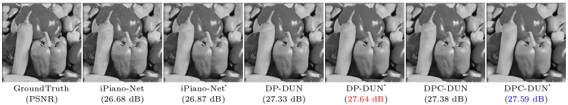
Figure 10: Visualization of noise robustness on Set11 dataset [25] when CS ratio = $10\%$ and $\sigma$ = 10, corresponding to Table X. Our DP-DUN and DPC-DUN produce fewer stains and more accurate edges without artifacts.

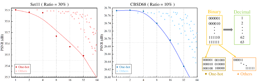
Figure 11: Scatter plots of the values in decimal format converted to binary and the corresponding PSNR values in two cases that are the same as Fig. 9.

IV-F1 Impact of Blocking Artifacts

To analyze the effect of image deblocking operations, we conduct the experiments of the models on Set11 dataset [25] in Table VIII, where “-” represents the results without finetuning on the patch size of $99\times 99$. After finetuning, our models get PSNR/SSIM gains, but the number of the active module ($N_{AM}$) does not change obviously, indicating that deblocking can achieve a better performance-consumption balance.

IV-F2 Application in the learnable sampling matrix

We use different sampling matrices to train our models to apply to different scenarios. We retrain DPC-DUN with the learnable matrix [65] and compare it with some recent methods which also jointly learn the sampling matrix and the reconstruction process. We present the performance comparisons on Set11 dataset in Table IX. Our methods can be well applied to this matrix with high robustness and achieve good performance.

IV-F3 Sensitivity to Noise

In the real application, the imaging model may be affected by noise, so we add the experiments of the models with various Gaussian noises on Set11 dataset [25] to demonstrate the robustness in Table X. We finetune ISTA-Net⁺ [28], iPiano-Net [43], DP-DUN, and DPC-DUN with the random noise in [0,10], namely ISTA-Net^+∗, iPiano-Net^∗, DP-DUN^∗, and DPC-DUN^∗ respectively. As shown in Table X, our proposed models outperform the compared methods with all noises. The PSNR differences of DP-DUN^∗/DPC-DUN^∗ between w/o noise ($\sigma=0$) and w/ noise are smaller than DP-DUN/DPC-DUN, which indicates that the models after finetuning are relatively robust to different noises, especially larger ones in testing. Therefore, our proposed method can tackle the compressive sensing problem with the corresponding settings and datasets in real applications. What is more, Fig. 10 shows the visual results of noise robustness, from which one can see that the texture of the image is smoother and the noise is less when the models are finetuned.

IV-F4 Analysis of Different Control Factors

Our DPC-DUN can dynamically balance the recovery accuracy and complexity by combining a one-hot vector encoded by the control factor $\mu$ and the input image feature. In this paper, $\mu$ is set to $\{0.00001,0.00005,0.0001,0.0005,0.001,0.002\}$ and corresponds to a one-hot vector $\{000001,000010,000100,001000,\\ 010000,100000\}$ as the input in the training phase. To break the limits of the six default one-hot vectors, we explore the effect of other (unseen) binary encoding vectors as the modulation during testing as shown in the lower row of Fig. 9 and find that all vectors have similar trends. To explore the relationship between vectors and the modulation mechanism, we compare the decimal numbers converted to binary numbers and the corresponding PSNR values in two cases, as shown in Fig. 11. Dots stand for the default settings, and triangles stand for the unseen settings. We can see that overall, the PSNR value decreases with the increase of the value in decimal format, and the default settings determine the extremum value of the reconstruction performance.

V Conclusion

We propose a Dynamic Path-Controllable Deep Unfolding Network (DPC-DUN) for image CS, which shows a slimming mechanism that dynamically selects different paths and enables model interactivity with controllable complexity. Utilizing the skip connection structure inherent in DUNs, our proposed Path-Controllable Selector (PCS) can adaptively choose to skip a different number of modules for the different input images, thereby reducing the computational cost while ensuring similar high performance. And PCS also artificially adjusts the performance-complexity tradeoff at test time conditioned on the Lagrange multiplier. Our work opens new angles for the modulation of different tradeoffs in the image inverse tasks. However, our method also has some limitations. First, some background details may still be over-smoothed by our method. Second, our selector is not fine-grained enough to judge the picture information. Lastly, our selector adjustment range is relatively small and not continuous, which does not have a high modulation accuracy. In the future, we will improve our work by adjusting the sampling rate and extending our DPC-DUN to other network structures and video applications.

Jiechong Song received the B.E. degree in the School of Electronics and Information Engineering, Sichuan University, Chengdu, China, in 2019. She is currently working toward a doctor’s degree in computer applications technology at Peking University Shenzhen Graduate School, Shenzhen, China. Her research interests include compressive sensing, image restoration, and computer vision.

Bin Chen received the B.E. degree in the School of Computer Science, Beijing University of Posts and Telecommunications, Beijing, China, in 2021. He is currently working toward the master’s degree in computer applications technology at Peking University Shenzhen Graduate School, Shenzhen, China. His research interests include compressive sensing, image restoration and computer vision.

Jian Zhang (M’14) received the B.S. degree from the Department of Mathematics, Harbin Institute of Technology (HIT), Harbin, China, in 2007, and received his M.Eng. and Ph.D. degrees from the School of Computer Science and Technology, HIT, in 2009 and 2014, respectively. From 2014 to 2018, he worked as a postdoctoral researcher at Peking University (PKU), Hong Kong University of Science and Technology (HKUST), and King Abdullah University of Science and Technology (KAUST). Currently, he is an Assistant Professor with the School of Electronic and Computer Engineering, Peking University Shenzhen Graduate School, Shenzhen, China. His research interests include intelligent multimedia processing, low-level vision and computational imaging. He is now leading the Visual-Information Intelligent Learning LAB (VILLA) at PKU. He has published over 90 technical articles in refereed international journals and proceedings, including SPM/TPAMI/TIP/CVPR/ECCV/ICCV/ICLR. He received the Best Paper Award at the 2011 IEEE Visual Communications and Image Processing (VCIP) and was a co-recipient of the Best Paper Award of 2018 IEEE MultiMedia.

References

- [1] J. Zhang, B. Chen, R. Xiong, and Y. Zhang, “Physics-inspired compressive sensing: Beyond deep unrolling,” IEEE Signal Processing Magazine, vol. 40, no. 1, pp. 58–72, 2023.
- [2] E. J. Candès, J. Romberg, and T. Tao, “Robust uncertainty principles: Exact signal reconstruction from highly incomplete frequency information,” IEEE Transactions on information theory, vol. 52, no. 2, pp. 489–509, 2006.
- [3] A. C. Sankaranarayanan, C. Studer, and R. G. Baraniuk, “CS-MUVI: Video compressive sensing for spatial-multiplexing cameras,” in Proceedings of the IEEE International Conference on Computational Photography (ICCP), Apr. 2012.
- [4] A. Liutkus, D. Martina, S. Popoff, G. Chardon, O. Katz, G. Lerosey, S. Gigan, L. Daudet, and I. Carron, “Imaging with nature: Compressive imaging using a multiply scattering medium,” Scientific Reports, vol. 4, p. 5552, 2014.
- [5] A. Zymnis, S. Boyd, and E. Candes, “Compressed sensing with quantized measurements,” IEEE Signal Processing Letters, vol. 17, no. 2, pp. 149–152, 2009.
- [6] T. P. Szczykutowicz and G. Chen, “Dual energy CT using slow kVp switching acquisition and prior image constrained compressed sensing,” Physics in Medicine & Biology, vol. 55, no. 21, p. 6411, 2010.
- [7] J. Zhang, Z. Zhang, J. Xie, and Y. Zhang, “High-throughput deep unfolding network for compressive sensing MRI,” IEEE Journal of Selected Topics in Signal Processing, vol. 16, no. 4, pp. 750–761, 2022.
- [8] Z. Chen, X. Hou, L. Shao, C. Gong, X. Qian, Y. Huang, and S. Wang, “Compressive sensing multi-layer residual coefficients for image coding,” IEEE Transactions on Circuits and Systems for Video Technology, vol. 30, no. 4, pp. 1109–1120, 2019.
- [9] M. F. Duarte, M. A. Davenport, D. Takhar, J. N. Laska, T. Sun, K. F. Kelly, and R. G. Baraniuk, “Single-pixel imaging via compressive sampling,” IEEE Signal Processing Magazine, vol. 25, no. 2, pp. 83–91, 2008.
- [10] F. Rousset, N. Ducros, A. Farina, G. Valentini, C. D’Andrea, and F. Peyrin, “Adaptive basis scan by wavelet prediction for single-pixel imaging,” IEEE Transactions on Computational Imaging, vol. 3, no. 1, pp. 36–46, 2016.
- [11] H. Shen, X. Li, L. Zhang, D. Tao, and C. Zeng, “Compressed sensing-based inpainting of aqua moderate resolution imaging spectroradiometer band 6 using adaptive spectrum-weighted sparse Bayesian dictionary learning,” IEEE Transactions on Geoscience and Remote Sensing, vol. 52, no. 2, pp. 894–906, 2013.
- [12] C. Mou and J. Zhang, “TransCL: Transformer makes strong and flexible compressive learning,” IEEE Transactions on Pattern Analysis and Machine Intelligence, vol. 45, no. 4, pp. 5236–5251, 2023.
- [13] Z. Wu, Z. Zhang, J. Song, and J. Zhang, “Spatial-temporal synergic prior driven unfolding network for snapshot compressive imaging,” in Proceedings of IEEE International Conference on Multimedia and Expo (ICME), Jul. 2021.
- [14] Z. Wu, J. Zhang, and C. Mou, “Dense deep unfolding network with 3D-CNN prior for snapshot compressive sensing,” in Proceedings of the IEEE International Conference on Computer Vision (ICCV), Oct. 2021, pp. 4892–4901.
- [15] Y. Kim, M. S. Nadar, and A. Bilgin, “Compressed sensing using a Gaussian scale mixtures model in wavelet domain,” in Proceedings of the IEEE International Conference on Image Processing (ICIP), Sep 2010, pp. 3365–3368.
- [16] C. Li, W. Yin, H. Jiang, and Y. Zhang, “An efficient augmented lagrangian method with applications to total variation minimization,” Computational Optimization and Applications, vol. 56, no. 3, pp. 507–530, 2013.
- [17] J. Zhang, D. Zhao, and W. Gao, “Group-based sparse representation for image restoration,” IEEE Transactions on Image Processing, vol. 23, no. 8, pp. 3336–3351, 2014.
- [18] J. Zhang, C. Zhao, D. Zhao, and W. Gao, “Image compressive sensing recovery using adaptively learned sparsifying basis via L0 minimization,” Signal Processing, vol. 103, pp. 114–126, 2014.
- [19] X. Gao, J. Zhang, W. Che, X. Fan, and D. Zhao, “Block-based compressive sensing coding of natural images by local structural measurement matrix,” in Proceedings of Data Compression Conference (DCC), Apr. 2015, pp. 133–142.
- [20] C. A. Metzler, A. Maleki, and R. G. Baraniuk, “From denoising to compressed sensing,” IEEE Transactions on Information Theory, vol. 62, no. 9, pp. 5117–5144, 2016.
- [21] C. Zhao, J. Zhang, R. Wang, and W. Gao, “CREAM: CNN-REgularized ADMM framework for compressive-sensed image reconstruction,” IEEE Access, vol. 6, pp. 76 838–76 853, 2018.
- [22] C. Zhao, S. Ma, and W. Gao, “Image compressive-sensing recovery using structured laplacian sparsity in DCT domain and multi-hypothesis prediction,” in Proceedings of IEEE International Conference on Multimedia and Expo (ICME), Jul. 2014.
- [23] C. Zhao, S. Ma, J. Zhang, R. Xiong, and W. Gao, “Video compressive sensing reconstruction via reweighted residual sparsity,” IEEE Transactions on Circuits and Systems for Video Technology, vol. 27, no. 6, pp. 1182–1195, 2016.
- [24] C. Zhao, J. Zhang, S. Ma, and W. Gao, “Nonconvex Lp nuclear norm based ADMM framework for compressed sensing,” in Proceedings of Data Compression Conference (DCC), Apr. 2016, pp. 161–170.
- [25] K. Kulkarni, S. Lohit, P. Turaga, R. Kerviche, and A. Ashok, “ReconNet: Non-iterative reconstruction of images from compressively sensed measurements,” in Proceedings of the IEEE Conference on Computer Vision and Pattern Recognition (CVPR), Jun. 2016, pp. 449–458.
- [26] Y. Sun, J. Chen, Q. Liu, B. Liu, and G. Guo, “Dual-path attention network for compressed sensing image reconstruction,” IEEE Transactions on Image Processing, vol. 29, pp. 9482–9495, 2020.
- [27] C. Ren, X. He, C. Wang, and Z. Zhao, “Adaptive consistency prior based deep network for image denoising,” in Proceedings of the IEEE Conference on Computer Vision and Pattern Recognition (CVPR), Jun. 2021, pp. 8596–8606.
- [28] J. Zhang and B. Ghanem, “ISTA-Net: Interpretable optimization-inspired deep network for image compressive sensing,” in Proceedings of the IEEE Conference on Computer Vision and Pattern Recognition (CVPR), Jun. 2018, pp. 1828–1837.
- [29] J. Zhang, C. Zhao, and W. Gao, “Optimization-inspired compact deep compressive sensing,” IEEE Journal of Selected Topics in Signal Processing, vol. 14, no. 4, pp. 765–774, 2020.
- [30] D. You, J. Xie, and J. Zhang, “ISTA-Net++: Flexible deep unfolding network for compressive sensing,” in Proceedings of IEEE International Conference on Multimedia and Expo (ICME), Jul. 2021.
- [31] D. You, J. Zhang, J. Xie, B. Chen, and S. Ma, “COAST: Controllable arbitrary-sampling network for compressive sensing,” IEEE Transactions on Image Processing, vol. 30, pp. 6066–6080, 2021.
- [32] Z. Zhang, Y. Liu, J. Liu, F. Wen, and C. Zhu, “AMP-Net: Denoising-based deep unfolding for compressive image sensing,” IEEE Transactions on Image Processing, vol. 30, pp. 1487–1500, 2020.
- [33] Y. Chen and T. Pock, “Trainable nonlinear reaction diffusion: A flexible framework for fast and effective image restoration,” IEEE Transactions on Pattern Analysis and Machine Intelligence, vol. 39, no. 6, pp. 1256–1272, 2016.
- [34] S. Lefkimmiatis, “Non-local color image denoising with convolutional neural networks,” in Proceedings of the IEEE Conference on Computer Vision and Pattern Recognition (CVPR), Jul. 2017, pp. 3587–3596.
- [35] J. Kruse, C. Rother, and U. Schmidt, “Learning to push the limits of efficient FFT-based image deconvolution,” in Proceedings of the IEEE International Conference on Computer Vision (ICCV), Oct. 2017, pp. 4596–4604.
- [36] H. Wang, T. Zhang, M. Yu, J. Sun, W. Ye, C. Wang, and S. Zhang, “Stacking networks dynamically for image restoration based on the plug-and-play framework,” in Proceedings of the European Conference on Computer Vision (ECCV), Aug. 2020, pp. 446–462.
- [37] F. Kokkinos and S. Lefkimmiatis, “Deep image demosaicking using a cascade of convolutional residual denoising networks,” in Proceedings of the European Conference on Computer Vision (ECCV), Sep. 2018, pp. 317–333.
- [38] K. Zhang, W. Zuo, S. Gu, and L. Zhang, “Learning deep CNN denoiser prior for image restoration,” in Proceedings of the IEEE Conference on Computer Vision and Pattern Recognition (CVPR), Jul. 2017, pp. 3929–3938.
- [39] W. Dong, P. Wang, W. Yin, G. Shi, F. Wu, and X. Lu, “Denoising prior driven deep neural network for image restoration,” IEEE Transactions on Pattern Analysis and Machine Intelligence, vol. 41, no. 10, pp. 2305–2318, 2018.
- [40] D. Gilton, G. Ongie, and R. Willett, “Neumann networks for linear inverse problems in imaging,” IEEE Transactions on Computational Imaging, vol. 6, pp. 328–343, 2019.
- [41] J. Song, B. Chen, and J. Zhang, “Memory-augmented deep unfolding network for compressive sensing,” in Proceedings of the ACM International Conference on Multimedia (ACM MM), Oct. 2021, pp. 4249–4258.
- [42] J. Chen, Y. Sun, Q. Liu, and R. Huang, “Learning memory augmented cascading network for compressed sensing of images,” in Proceedings of the European Conference on Computer Vision (ECCV), Aug. 2020, pp. 513–529.
- [43] Y. Su and Q. Lian, “iPiano-Net: Nonconvex optimization inspired multi-scale reconstruction network for compressed sensing,” Signal Processing: Image Communication, vol. 89, p. 115989, 2020.
- [44] K. Yu, X. Wang, C. Dong, X. Tang, and C. C. Loy, “Path-Restore: Learning network path selection for image restoration,” IEEE Transactions on Pattern Analysis and Machine Intelligence, vol. 44, no. 10, pp. 7078–7092, 2021.
- [45] Y. Han, G. Huang, S. Song, L. Yang, H. Wang, and Y. Wang, “Dynamic neural networks: A survey,” IEEE Transactions on Pattern Analysis and Machine Intelligence, vol. 44, no. 11, pp. 7436–7456, 2021.
- [46] M. Zhu, K. Han, E. Wu, Q. Zhang, Y. Nie, Z. Lan, and Y. Wang, “Dynamic resolution network,” in Proceedings of the International Conference on Neural Information Processing Systems (NeurIPS), Dec. 2021.
- [47] C. Li, G. Wang, B. Wang, X. Liang, Z. Li, and X. Chang, “Dynamic slimmable network,” in Proceedings of the IEEE Conference on Computer Vision and Pattern Recognition (CVPR), Jun. 2021, pp. 8607–8617.
- [48] Z. Wu, T. Nagarajan, A. Kumar, S. Rennie, L. S. Davis, K. Grauman, and R. Feris, “BlockDrop: Dynamic inference paths in residual networks,” in Proceedings of the IEEE Conference on Computer Vision and Pattern Recognition (CVPR), Jun. 2018, pp. 8817–8826.
- [49] X. Wang, F. Yu, Z.-Y. Dou, T. Darrell, and J. E. Gonzalez, “SkipNet: Learning dynamic routing in convolutional networks,” in Proceedings of the European Conference on Computer Vision (ECCV), Sep. 2018, pp. 420–436.
- [50] Y. Song, Y. Zhu, and X. Du, “Dynamic residual dense network for image denoising,” Sensors, vol. 19, no. 17, p. 3809, 2019.
- [51] K. He, X. Zhang, S. Ren, and J. Sun, “Deep residual learning for image recognition,” in Proceedings of the IEEE Conference on Computer Vision and Pattern Recognition (CVPR), Jun. 2016, pp. 770–778.
- [52] J. He, C. Dong, Y. Liu, and Y. Qiao, “Interactive multi-dimension modulation for image restoration,” IEEE Transactions on Pattern Analysis and Machine Intelligence, vol. 44, no. 12, pp. 9363–9379, 2021.
- [53] H. Cai, J. He, Y. Qiao, and C. Dong, “Toward interactive modulation for photo-realistic image restoration,” in Proceedings of the IEEE Conference on Computer Vision and Pattern Recognition Workshops (CVPRW), Jun. 2021.
- [54] J. Jiang, K. Zhang, and R. Timofte, “Towards flexible blind JPEG artifacts removal,” in Proceedings of the IEEE International Conference on Computer Vision (ICCV), Oct. 2021, pp. 4977–4986.
- [55] Y. Choi, M. El-Khamy, and J. Lee, “Variable rate deep image compression with a conditional autoencoder,” in Proceedings of the IEEE Conference on Computer Vision and Pattern Recognition (CVPR), Jun. 2019, pp. 3146–3154.
- [56] J. Lin, M. Akbari, H. Fu, Q. Zhang, S. Wang, J. Liang, D. Liu, F. Liang, G. Zhang, and C. Tu, “Variable-rate multi-frequency image compression using modulated generalized octave convolution,” in Proceedings of the International Workshop on Multimedia Signal Processing (MMSP), Sep. 2020.
- [57] E. Jang, S. Gu, and B. Poole, “Categorical reparameterization with Gumbel-Softmax,” in Proceedings of the International Conference on Learning Representations (ICLR), Apr. 2017.
- [58] T. Dai, Y. Lv, B. Chen, Z. Wang, Z. Zhu, and S.-T. Xia, “Mix-order attention networks for image restoration,” in Proceedings of the ACM International Conference on Multimedia (ACM MM), Oct. 2021, pp. 2880–2888.
- [59] J. Hu, L. Shen, and G. Sun, “Squeeze-and-excitation networks,” in Proceedings of the IEEE Conference on Computer Vision and Pattern Recognition (CVPR), Jun. 2018, pp. 7132–7141.
- [60] K. Zhang, Y. Li, W. Zuo, L. Zhang, L. Van Gool, and R. Timofte, “Plug-and-play image restoration with deep denoiser prior,” IEEE Transactions on Pattern Analysis and Machine Intelligence, vol. 44, no. 10, pp. 6360–6376, 2021.
- [61] E. Agustsson and R. Timofte, “NTIRE 2017 challenge on single image super-resolution: Dataset and study,” in Proceedings of the IEEE Conference on Computer Vision and Pattern Recognition Workshops (CVPRW), Jul. 2017.
- [62] Y. Zhong, C. Zhang, F. Ren, H. Kuang, and P. Tang, “Scalable image compressed sensing with generator networks,” IEEE Transactions on Computational Imaging, vol. 8, pp. 1025–1037, 2022.
- [63] C. Ma, J. T. Zhou, X. Zhang, and Y. Zhou, “Deep unfolding for compressed sensing with denoiser,” in Proceedings of IEEE International Conference on Multimedia and Expo (ICME), Jul. 2022.
- [64] M. Shen, H. Gan, C. Ning, Y. Hua, and T. Zhang, “TransCS: A transformer-based hybrid architecture for image compressed sensing,” IEEE Transactions on Image Processing, vol. 31, pp. 6991–7005, 2022.
- [65] W. Shi, F. Jiang, S. Liu, and D. Zhao, “Image compressed sensing using convolutional neural network,” IEEE Transactions on Image Processing, vol. 29, pp. 375–388, 2019.