Unimodal measurable pseudo-Anosov maps

Abstract.

We exhibit a continuously varying family $F_{\lambda}$ of homeomorphisms of the sphere $S^{2}$, for which each $F_{\lambda}$ is a measurable pseudo-Anosov map. Measurable pseudo-Anosov maps are generalizations of Thurston’s pseudo-Anosov maps, and also of the generalized pseudo-Anosov maps of [22]. They have a transverse pair of invariant full measure turbulations, consisting of streamlines which are dense injectively immersed lines: these turbulations are equipped with measures which are expanded and contracted uniformly by the homeomorphism. The turbulations need not have a good product structure anywhere, but have some local structure imposed by the existence of tartans: bundles of unstable and stable streamline segments which intersect regularly, and on whose intersections the product of the measures on the turbulations agrees with the ambient measure.

Each map $F_{\lambda}$ is semi-conjugate to the inverse limit of the core tent map with slope $\lambda$: it is topologically transitive, ergodic with respect to a background Oxtoby-Ulam measure, has dense periodic points, and has topological entropy $h(F_{\lambda})=\log\lambda$ (so that no two $F_{\lambda}$ are topologically conjugate). For a full measure, dense $G_{\delta}$ set of parameters, $F_{\lambda}$ is a measurable pseudo-Anosov map but not a generalized pseudo-Anosov map, and its turbulations are nowhere locally regular.

1. Introduction

Since their introduction by Thurston in the 1970s, pseudo-Anosov maps have played a central rôle in low-dimensional geometry and topology, but also in low-dimensional dynamics. In the former area, pseudo-Anosov maps first appeared in Thurston’s Classification Theorem for isotopy classes of surface homeomorphisms. They are also fundamental for the statement and the proof of Thurston’s Hyperbolization Theorem for fibered 3-manifolds. In both of these discussions, there is a finiteness hypothesis: the surfaces involved are of finite topological type, that is, they are compact surfaces from which finitely many points have been removed, or marked.

In surface dynamics, the way that pseudo-Anosov maps appear is, most often, as follows: given a homeomorphism $f$ of a surface $S$, find a periodic orbit $O$ and apply the Classification Theorem to $f$ on $S\setminus O$; if this isotopy class is pseudo-Anosov then one can conclude, amongst other things, that $f$ has infinitely many other periodic orbits, of infinitely many distinct periods, and has positive topological entropy. If we adopt the point of view that the periodic orbit $O$ consists of marked points instead of having been removed (in which case only isotopies relative to $O$ are allowed), we can consider the collection $\operatorname{pA}(S)$ of all pseudo-Anosov homeomorphisms on a given surface $S$, relative to all possible finite invariant sets and up to topological changes of coordinates. Since, up to changes of coordinates, pseudo-Anosov maps are unique in a given marked isotopy class, the set $\operatorname{pA}(S)$ is countable. At this point some questions arise naturally. What kind of set is $\operatorname{pA}(S)$? How does it sit inside the set $\operatorname{Homeo}(S)$ of all homeomorphisms of $S$? Can we complete it somehow, and what sort of maps would be necessary to do this? To the best of our knowledge the nature of $\operatorname{pA}(S)$ as a subset of $\operatorname{Homeo}(S)$ remains a puzzle, and none of these questions has a satisfactory answer. In the remainder of the introduction we describe the pieces of this puzzle which are already in place, and the new ones which we will fit to it here.

There is a well-known and useful interplay between three distinct versions or models of pseudo-Anosov maps:

• The pseudo-Anosov map itself fills its surface of definition with transitive dynamics. There is an ergodic invariant measure of full support, and a transverse pair of invariant measured foliations of the surface, one expanded and one contracted by the map. We are primarily interested in pseudo-Anosov maps on a fixed surface such as $S^{2}$, relative to finite invariant sets, at which points the foliations may have one-pronged singularities. The invariant measured foliations endow the surface with a Euclidean structure with finitely many cone points, with cone angles multiples of $\pi$. Moreover, they also define horizontal and vertical directions of this Euclidean structure with respect to which the pseudo-Anosov map is linear, with diagonal matrix of the form $\left(\begin{smallmatrix}\lambda&0\\ 0&\lambda^{-1}\end{smallmatrix}\right)$, where $\lambda>1$ is the pseudo-Anosov dilatation factor and $\log\lambda$ is its topological entropy.

• The second version is produced by the DA procedure. By locally pushing out at the singularities of the foliations, the transitive dynamics collapses onto a one-dimensional hyperbolic attractor. The unstable foliation becomes a lamination of the attractor by unstable manifolds and the stable foliation becomes the stable manifolds of the attractor. The pseudo-Anosov map can be recovered by carefully collapsing complementary regions of the attractor.

• The third version is constructed by a further collapse down pieces of the stable manifolds, which yields an expanding map on a one-dimensional branched manifold, called an invariant train track. The attractor version can be recovered by taking an inverse limit.

A result of Bonatti and Jeandenans (see the appendix of [9]) relates pseudo-Anosov maps to differentiable dynamics: they show that there is a natural quotient of a Smale (Axiom A + strong transversality) surface diffeomorphism without impasses (bigons bounded by a stable segment and an unstable segment) which is pseudo-Anosov. This result has recently been generalized by Mello [30], who showed that, when impasses are allowed, the quotient map is a generalized pseudo-Anosov map. These are surface homeomorphisms analogous to pseudo-Anosov maps, except that the invariant foliations are allowed to have countably many singularities, accumulating on finitely many ‘bad points’ (see Definitions 2.8 below). As in the pseudo-Anosov case, the invariant measured foliations endow the surface with a Euclidean structure (with cone points and with finitely many accumulations of cone points) and become horizontal and vertical lines of this structure. In these coordinates, the generalized pseudo-Anosov map is locally diagonal linear, with constant expansion and contraction factors $\lambda$ and $\lambda^{-1}$, where $\log\lambda$ is the topological entropy. The quotient maps relating the Smale diffeomorphisms to their generalized pseudo-Anosov quotients are dynamically mild in the sense that fibers carry no entropy.

Together, these results indicate that pseudo-Anosov and generalized pseudo-Anosov maps can be viewed as linear models with constant expansion and contraction constants for Smale surface diffeomorphisms. This places pseudo-Anosov and generalized pseudo-Anosov maps in a broader context in the study of surface dynamics, but the results of Bonatti-Jeandenans and Mello only apply to hyperbolic diffeomorphisms. Since both collections of maps — Smale surface diffeomorphisms and pseudo-Anosov maps — are countable up to changes of coordinates, this semi-conjugacy from the differentiable world to the pseudo-Anosov world cannot exist for all maps in a parametrized family of diffeomorphisms, such as the Hénon family.

There has been some recent success in moving parts of this discussion beyond the context of hyperbolic dynamics. Crovisier and Pujals [21] show that for a large set of parameters in the Hénon family, collapsing down local stable sets yields a map on a dendrite. Boroński and Štimac [10] prove a similar result for the Lozi family and show that, in both the Hénon and Lozi cases, for certain parameter sets, the attractor is conjugate to the natural extension acting on the inverse limit of the associated dendrite map.

In the other direction, and much earlier, Barge and Martin [6] described a general procedure which starts with a self-map of a graph embedded in a surface, and yields a surface homeomorphism having an attractor on which the dynamics is conjugate to the natural extension of the graph map.

Our approach to understanding the puzzle of how $\operatorname{pA}(S)$ sits inside $\operatorname{Homeo}(S)$ is to construct a parametrized family $\left\{F_{\lambda}\colon\lambda\in(\sqrt{2},2]\right\}$ of homeomorphisms of $S^{2}$, which intersects $\operatorname{pA}(S^{2})$ in a countable set; to describe this intersection; and to describe the structure of the maps of $F_{\lambda}$ which are not in $\operatorname{pA}(S^{2})$, and how they are accumulated by pseudo-Anosov and generalized pseudo-Anosov maps in the family.

The first simplification is to restrict attention to a subset of $\operatorname{pA}(S^{2})$ and to consider only pseudo-Anosov maps of the sphere which occur as representatives in the isotopy class of Smale’s horseshoe map relative to one of its periodic orbits. If we denote this set by $\operatorname{HS}$, we can pose the same questions as above. What kind of set is $\operatorname{HS}$? How does it sit inside the set of all homeomorphisms of $S$? Can we complete it somehow, and what sort of maps would be necessary to do this? An understanding of these questions can be expected to illuminate the general case.

There is a natural correspondence between horseshoe periodic orbits and periodic orbits which occur in the tent family of interval endomorphisms. Symbolically, this is simply the fact that horseshoe orbits and tent orbits can both be coded by sequences of 0s and 1s: those of the horseshoe, which is an invertible map, are coded by bi-infinite sequences, whereas those of endomorphisms in the tent family are one-sided infinite. For periodic orbits, whether they are 1- or 2-sided is irrelevant, since they are determined by a finite, repeating, word: this establishes the desired correspondence.

The pieces of the puzzle previously put in place by the authors are mainly contained in the papers [25, 22, 23, 14]:

• The train tracks mentioned above are essentially graphs with added information at the vertices, and train track maps are Markov endomorphisms which respect this added information. In [25], the subset of $\operatorname{HS}$ whose invariant train tracks are intervals and invariant train track maps are tent maps was identified. It is parametrized by an invariant named height, which is a rational number in the interval $(0,\tfrac{1}{2})$.

• In [22], it was shown that, to every tent (or horseshoe) periodic orbit, there is associated a generalized pseudo-Anosov map of the 2-sphere whose dynamics mimics that of the corresponding tent map. These are called unimodal generalized pseudo-Anosov maps.

• The main application of the results of [23] was to conclude that a certain sequence of unimodal generalized pseudo-Anosov maps is convergent, having limit the tight horseshoe, a version of the horseshoe without wandering domains, but with the same dynamics otherwise.

• In [14] we showed how the Barge-Martin attractors built from the natural extensions of tent maps on the interval can be turned into transitive, area-preserving homeomorphisms of the 2-sphere. These homeomorphisms are semi-conjugate — by very mild semi-conjugacies — to the natural extensions of tent maps. Moreover, this yields a continuously varying family of sphere homeomorphisms and, although the construction is very different, this family contains all of the unimodal generalized pseudo-Anosov maps of [22]. In particular, in place of the single limit identified in [23], every map in this continuously varying family is a limit of unimodal generalized pseudo-Anosov maps.

The main aim of the current paper is to address the question: what sort of maps are these limits? We show that they have enough structure to make them deserve to be called measurable pseudo-Anosov maps. These are analogs of pseudo-Anosov maps in which the transverse pair of invariant measured foliations is replaced with a transverse pair of invariant measured turbulations: full measure subsets of the surface decomposed into a disjoint union of streamlines, which are injectively immersed lines equipped with measures. As in the pseudo-Anosov case, one of these turbulations is expanded and the other is contracted by the dynamics, by a constant factor which, in this setting, is the slope of the associated tent map. For particular values of the slope, this measurable pseudo-Anosov map may be a generalized pseudo-Anosov map or, occasionally, an honest-to-goodness pseudo-Anosov map.

Our main focus is on defining measurable pseudo-Anosov maps, and showing that they are fairly abundant in two-dimensional dynamics in the sense that they form a continuously varying family. In another paper [15], we show that the definition has dynamical weight by proving that any measurable pseudo-Anosov map is Devaney-chaotic (it has dense periodic points and is topologically transitive); and, under an additional hypothesis, is ergodic. (For the particular family discussed in this paper, these dynamical properties follow more directly from the construction.)

In defining measurable pseudo-Anosov maps we were predominantly guided by Thurston’s original definition of pseudo-Anosov maps, but also by the higher-dimensional (holomorphic) analogs in [8, 29, 34]. In particular, the term ‘turbulation’ is borrowed from comments in [29].

Before stating the results in more detail, we provide some preliminary definitions and notation: more details can be found in Sections 3.1 (tent maps), 3.2 (inverse limits), and 3.3 (invariant measures).

The core tent map $f_{\lambda}\colon I_{\lambda}\to I_{\lambda}$ with slope $\lambda\in(\sqrt{2},2]$ is the restriction of the full tent map $T_{\lambda}\colon[0,1]\to[0,1]$ defined by $T_{\lambda}(x)=\min(\lambda x,\lambda(1-x))$ to the interval $I_{\lambda}=\left[T_{\lambda}^{2}(1/2),T_{\lambda}(1/2)\right]$. It has turning or critical point $c=1/2$. For the vast majority of the paper we will only be concerned with single tent maps, so, except where absolutely necessary, the dependence of objects on the parameter $\lambda$ will be suppressed. The natural extension of the tent map, acting on its inverse limit, is denoted ${{\widehat{f}}}\colon{{\widehat{I}}}\to{{\widehat{I}}}$. We write $\pi_{0}\colon{{\widehat{I}}}\to I$ for the projection of the inverse limit onto its base using the $0^{\text{th}}$ coordinate, and $\left[x\right]:=\pi_{0}^{-1}(x)$ for the $\pi_{0}$-fiber of ${{\widehat{I}}}$ above a point $x\in I$.

As discussed above, it is shown in [14] that there is a map $g\colon{{\widehat{I}}}\to S^{2}$ which semi-conjugates ${{\widehat{f}}}\colon{{\widehat{I}}}\to{{\widehat{I}}}$ to a sphere homeomorphism $F\colon S^{2}\to S^{2}$ (and, momentarily restoring the dependence on the parameter, the sphere homeomorphisms $F_{\lambda}$ vary continuously with $\lambda$). The tent map $f$ has a unique ergodic invariant measure $\mu$ of maximal entropy, which is absolutely continuous with respect to Lebesgue measure. This measure gives rise to an ergodic ${{\widehat{f}}}$-invariant measure on the inverse limit, and in turn to a fully supported ergodic $F$-invariant one, also denoted $\mu$, on $S^{2}$. When we speak of full measure on $S^{2}$, it is always with respect to this measure (which depends, of course, on the parameter $\lambda$).

The behavior of the sphere homeomorphism $F$ depends on two pieces of information about the tent map $f$: its height, and the nature of the orbit of its turning point.

• The height can be defined dynamically either as the rotation number of the outside map, a circle endomorphism associated with $f$ (Section 4.2); or as the prime ends rotation number of the basin of infinity in the attractor model [14]. It can be computed directly from the kneading sequence of $f$, at least when it is rational [25]. It is a decreasing function of the parameter $\lambda$, with an interval of parameters corresponding to each rational height, and a single parameter corresponding to each irrational.

• As far as the orbit of the turning point is concerned, the main distinction is between the post-critically finite (where the orbit of $c$ is periodic or pre-periodic) and the post-critically infinite cases.

For a typical parameter $\lambda$, the tent map $f$ is post-critically infinite with rational height. In this case, the sphere homeomorphism is measurable pseudo-Anosov, but is neither pseudo-Anosov nor generalized pseudo-Anosov. It is important to understand that, even though the turbulations are of full measure and transverse to each other, their local structure can be very complicated: for example, when the critical orbit is dense, the streamlines which locally give a product structure are never locally of full measure, so that there are no local foliated charts anywhere on the sphere. Informally, the orbit of the critical fiber $\left[c\right]$ carries a ‘kink’ which precludes a local product structure at accumulation points.

The construction of the measurable pseudo-Anosov map proceeds as follows. The unstable streamlines correspond to the full measure collection of path components in the inverse limit which are dense injectively immersed lines (see [13]). The measure is locally the pull back of Lebesgue measure on the interval under the projection $\pi_{0}$. The stable turbulation is built using the fibers $\pi_{0}^{-1}(x)$ and measures $\alpha_{x}$ supported on these fibers, which were constructed in [13] using the density of the tent map absolutely continuous invariant measure of maximal entropy. Each fiber is a Cantor set, and all but countably many of them project to an arc in the sphere carrying the push forward of $\alpha_{x}$. The ends of all but countably many of these arcs are connected in pairs by the semi-conjugacy $g$. The countable collection of non-conforming fibers/arcs are omitted from the stable turbulation.

While we obtain a reasonably nice global structure on a set of full measure, the inverse limits in this case are known to be exquisitely complicated topological objects. For example, when the parameter $\lambda$ is such that critical orbit is dense (these parameters are contained in the rational height, post-critically infinite case), theorems of Bruin and of Raines imply that the inverse limit ${{\widehat{I}}}_{\lambda}$ is nowhere locally the product of a Cantor set and an interval [19, 32]. Even more striking is that, for a perhaps smaller, but still dense $G_{\delta}$ set of parameters, Barge, Brucks and Diamond [4] (see also [1]) show that the inverse limit has a strong self-similarity: every open subset of ${{\widehat{I}}}_{\lambda}$ contains a homeomorphic copy of ${{\widehat{I}}}_{t}$ for every $t\in(\sqrt{2},2]$.

In the other cases of the height and critical orbit data, the construction follows the same general outline, but there is more regularity and the sphere homeomorphism $F_{\lambda}$ is generalized pseudo-Anosov.

• When the height is irrational (which implies that the tent map is post-critically infinite); or when $\lambda$ is an endpoint of a rational height interval (which implies that the tent map is post-critically finite), there is a single bad point (accumulation of singularities) $\infty$, and a single orbit of one-pronged singularities which is homoclinic to it: all other points are regular points of the invariant foliations.

• When $\lambda$ is in the interior of a rational height interval and the tent map is post-critically finite, then, with the exception of a single parameter $\lambda$ in each rational height interval, there is a fixed bad point $\infty$ and a further periodic orbit $Q$ of bad points having the same period as the post-critical periodic orbit. Heteroclinic orbits of connected one-pronged and three-pronged singularities emerge from $\infty$ and converge to $Q$.

  For the exceptional parameter $\lambda$ in each rational height interval, the sphere homeomorphism $F_{\lambda}$ is pseudo-Anosov.

The following theorem summarizes the properties of the family.

Theorem.

There exists a continuously varying family of sphere homeomorphisms $F_{\lambda}:S^{2}\to S^{2}$ for $\lambda\in(\sqrt{2},2]$ such that

• There is a continuous surjection $g_{\lambda}\colon{{\widehat{I}}}_{\lambda}\to S^{2}$, which semi-conjugates the natural extension ${{\widehat{f}}}_{\lambda}$ of the core tent map $f_{\lambda}$ to $F_{\lambda}$.

• $F_{\lambda}$ is a measurable pseudo-Anosov map with dilatation $\lambda$.

• For a countable discrete set of parameters, $F_{\lambda}$ is pseudo-Anosov.

• For an uncountable dense set of parameters, $F_{\lambda}$ is generalized pseudo-Anosov.

• For a dense $G_{\delta}$, full measure set of parameters, $F_{\lambda}$ is not generalized pseudo-Anosov, its invariant turbulations are nowhere locally regular, and the complement of its unstable turbulation contains a dense $G_{\delta}$ set.

• Each $F_{\lambda}$ is topologically transitive, ergodic with respect to a background Oxtoby-Ulam measure, has dense periodic points, and has topological entropy $h(F_{\lambda})=\log\lambda$ (so that no two $F_{\lambda}$ are topologically conjugate).

Our results relate to a specific family of measurable pseudo-Anosov maps, but they raise a number of questions of a more general nature. In [22] it was shown that the generalized pseudo-Anosov maps considered here are quasi-conformal with respect to a complex structure on the sphere, and that the invariant foliations are trajectories of an integrable quadratic differential. Does any of this structure exist for the more general measurable pseudo-Anosov maps and, if it does, is the quasi-conformal distortion of $F_{\lambda}$ equal to $\lambda$? A related question is whether or not measurable pseudo-Anosov maps are smoothable: topologically conjugate to, say, a $C^{k}$-diffeomorphism, for some $k\geq 1$? Another natural question concerns their prevalence amongst surface homeomorphisms. In our setting the measurable pseudo-Anosov maps occur in a continuous one-parameter family containing a countable family of pseudo-Anosov maps. How common is this: for example, given two isotopic pseudo-Anosov maps (necessarily relative to finite invariant sets), is there a continuous generic one-parameter family connecting them which consists solely of measurable pseudo-Anosov maps? More generally, is the collection of measurable pseudo-Anosov maps in some sense the completion of the collection of generalized pseudo-Anosov maps?

In Section 2 we define measurable pseudo-Anosov maps and prove some basic properties. Because the invariant turbulations of a measurable pseudo-Anosov map need not have a local product structure anywhere, their associated measures are defined on streamlines rather than on transverse arcs. For consistency we take the same approach with the measures on (generalized) pseudo-Anosov foliations, and these alternative definitions are also given in Section 2. Section 3 is a review of some necessary background material on tent maps, their invariant measures, and their inverse limits. Section 4 contains the main theoretical content of the paper: we discuss the structure of $\pi_{0}$-fibers of inverse limits of tent maps, identify their extreme elements, and model the action of the natural extension on these extreme elements by means of a circle map called the outside map. In Sections 5 and 6 we apply this first to the post-critically infinite rational height case and then to the irrational height case, proving that the associated sphere homeomorphisms are measurable pseudo-Anosov maps and generalized pseudo-Anosov maps respectively. The paper ends with a brief summary of how the post-critically finite rational case could be treated using the same approach: we omit the details because the fact that the sphere homeomorphisms associated to these tent maps are generalized pseudo-Anosov maps was proved, using quite different techniques, in [14].

2. Generalized and measurable pseudo-Anosov maps

We will show that the sphere homeomorphisms $F_{\lambda}$ are either examples of Thurston’s pseudo-Anosov maps [35], or one of two successive generalizations of them: the generalized pseudo Anosov maps of [22], which are permitted to have infinitely many pronged singularities, provided that these only accumulate at finitely many points; and measurable pseudo-Anosov maps, which have invariant measured turbulations, rather than foliations. A measured turbulation (Definitions 2.11) is a partition of a full measure subset of the sphere into streamlines: immersed lines equipped with measures, which play the rôle of the leaves of a foliation.

Because the invariant turbulations of a measurable pseudo-Anosov map may not have a local product structure in any open set, it is necessary to define the associated measures on the streamlines, rather than on arcs transverse to them. For this reason, and for the sake of consistency, we take the same approach with the measures for pseudo-Anosov and generalized pseudo-Anosov foliations.

We start by defining local models for regular and singular points of pseudo-Anosov and generalized pseudo-Anosov maps. These models come equipped with measures not only on the domain, but also on each stable and unstable leaf segment. Note that the invariant measured foliations will be defined globally, with the local models serving only to ensure that they have the desired local structure: thus no transition conditions are required where the local models overlap.

Because measurable pseudo-Anosov maps cannot be defined using local models for their invariant turbulations, properties such as holonomy invariance of the measures and their compatibility with the ambient measure are expressed instead in terms of tartans (Definitions 2.15): unions of stable and unstable arcs which intersect regularly, each stable arc intersecting each unstable arc exactly once.

Remark 2.1.

When we say that a subset of a topological space is measurable, it will always mean with respect to the Borel $\sigma$-algebra.

2.1. Pseudo-Anosov and Generalized pseudo-Anosov maps

Definition 2.2 (regular model).

Let $I$ and $J$ be intervals in ${{\mathbb{R}}}$. We denote by $R_{I,J}$ the rectangle $I\times J$ in ${{\mathbb{R}}}^{2}$, equipped with two-dimensional Lebesgue measure $M$, and refer to it as a regular model. Each horizontal $I\times\{\beta\}$ in $R_{I,J}$ is called an unstable leaf segment, and is equipped with one-dimensional Lebesgue measure $m_{u}$; similarly, each vertical $\{\alpha\}\times J$, with one-dimensional Lebesgue measure $m_{s}$, is called a stable leaf segment.

Definition 2.3 ($p$-pronged model, see Figure 1).

Given $a,b>0$ and $p\in{{\mathbb{Z}}}_{+}\setminus\{2\}$, we denote by $Q_{p,a,b}$ the space obtained from $p$ copies $R_{0},\dots,R_{p-1}$ of $(-a,a)\times[0,b)$ by identifying $(\alpha,0)\in R_{i}$ with $(-\alpha,0)\in R_{i+1\bmod{p}}$ for each $\alpha\in[0,a)$ and $i\in\{0,\dots,p-1\}$, and refer to it as a $p$-pronged model. We equip $Q_{p,a,b}$ with the measure $M$ induced by Lebesgue measure on each $R_{i}$. We say that the point obtained by identification of $(0,0)\in R_{i}$ for all $i$ is the singular point of the model.

An unstable leaf segment in $Q_{p,a,b}$ is either a segment $(-a,a)\times\{\beta\}$ in some $R_{i}$ for $\beta\in(0,b)$; or the union of the segments $[0,a)\times\{0\}$ in each $R_{i}$ after identifications. A stable leaf segment in $Q_{p,a,b}$ is either the union (after identifications) of $\{\alpha\}\times[0,b)$ in $R_{i}$ and $\{-\alpha\}\times[0,b)$ in $R_{i+1\bmod{p}}$ for some $\alpha\in(0,a)$; or the union of $\{0\}\times[0,b)$ in $R_{i}$ over all $i$. Unstable and stable leaf segments are equipped with the measures $m_{u}$ and $m_{s}$ induced by disintegration of $M$.

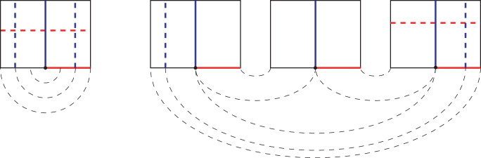
Figure 1. A 1-pronged model and a 3-pronged model, each with two unstable (red) and two stable (blue) leaf segments. The dashed leaf segments are arcs, while the solid ones, which pass through the singular point of the model, are 1-ods and 3-ods. The curved dashed lines denote identifications

Definition 2.4 (OU).

We say that a measure $\mu$ on a topological space $X$ is OU (for Oxtoby-Ulam) if it is Borel, non-atomic, and positive on open subsets of $X$. If $X$ is a compact manifold, then it is further required that $\mu(\partial X)=0$.

Throughout the remainder of this section, we let $\Sigma$ be a surface, and $\mu$ be an OU probability measure on $\Sigma$.

Note that the following definition of a measured foliation on $\Sigma$ makes little sense in isolation (since there is no requirement for measures on distinct leaves to be compatible), and will only take on a proper meaning when constraints on the local structure are introduced in Definitions 2.7. Note also that it is not the standard definition: as explained above, we put measures on the leaves rather than on arcs transverse to them, for consistency with the definition of measurable pseudo-Anosov turbulations.

Definition 2.5 (measured foliation, image foliation).

A measured foliation $({{\mathcal{F}}},\nu)$ on $\Sigma$ is a partition ${{\mathcal{F}}}$ of $\Sigma$ into subsets called leaves, together with an OU measure $\nu_{\ell}$ on each non-singleton leaf $\ell$. If $F\colon\Sigma\to\Sigma$ is a homeomorphism, we write $F({{\mathcal{F}}},\nu)$ for the measured foliation $({{\mathcal{F}}}^{\prime},\nu^{\prime})$ whose leaves are $\{F(\ell)\,:\,\ell\in{{\mathcal{F}}}\}$, with measures $\nu^{\prime}_{F(\ell)}=F_{*}(\nu_{\ell})$ on non-singleton leaves.

Note that, while $\mu$ is a probability measure, there is no requirement for the leaf measures $\nu_{\ell}$ to be finite, and they will generally not be.

Definitions 2.6 (regular and $p$-pronged charts).

Let $({{\mathcal{F}}}^{s},\nu^{s})$ and $({{\mathcal{F}}}^{u},\nu^{u})$ be measured foliations on $\Sigma$, and let $x\in\Sigma$. We say that the foliations have a regular chart at $x$ if there is a neighborhood $N$ of $x$, a regular model $R=R_{I,J}$, and a measure-preserving homeomorphism $\Phi\colon N\to R$, such that for each $\ell\in{{\mathcal{F}}}^{s}$ (respectively $\ell\in{{\mathcal{F}}}^{u}$), and each path component $L$ of $\ell\cap N$, $\Phi|_{L}$ is a measure-preserving homeomorphism onto a stable (respectively unstable) leaf segment of $R$. (To be clear, that $\Phi$ is measure-preserving means that $\Phi_{*}(\mu)=M$; and that $\Phi|_{L}$ is measure-preserving means that $(\Phi|_{L})_{*}(\nu_{\ell}^{s/u})=m_{s/u}$.)

We say that the foliations have a $p$-pronged chart at $x$ if there is a neighborhood $N$ of $x$, a $p$-pronged model $Q=Q_{p,a,b}$, and a measure-preserving homeomorphism $\Phi\colon N\to Q$, with $\Phi(x)$ the singular point of $Q$, such that for each $\ell\in{{\mathcal{F}}}^{s}$ (respectively $\ell\in{{\mathcal{F}}}^{u}$), and each path component $L$ of $\ell\cap N$, $\Phi|_{L}$ is a measure-preserving homeomorphism onto a stable (respectively unstable) leaf segment of $Q$.

Definitions 2.7 (pseudo-Anosov and generalized pseudo-Anosov foliations).

Let $({{\mathcal{F}}}^{s},\nu^{s})$ and $({{\mathcal{F}}}^{u},\nu^{u})$ be measured foliations on $\Sigma$. We say that they are pseudo-Anosov foliations if they have regular charts at all but finitely many points of $\Sigma$, and at each other point they have a pronged chart. We say that they are generalized pseudo-Anosov foliations if there is a countable $Y\subset\Sigma$ and a finite $Z\subset\Sigma\setminus Y$ such that the foliations have regular charts at every point of $\Sigma\setminus(Y\cup Z)$; pronged charts at every point of $Y$; and each point of $Z$ is a singleton leaf of both foliations.

Definitions 2.8 (pseudo-Anosov and generalized pseudo-Anosov maps).

Let $F\colon\Sigma\to\Sigma$ be a homeomorphism. We say that $F$ is (generalized) pseudo-Anosov if there are (generalized) pseudo-Anosov foliations $({{\mathcal{F}}}^{s},\nu^{s})$ and $({{\mathcal{F}}}^{u},\nu^{u})$ on $\Sigma$ and a number $\lambda>1$ such that $F({{\mathcal{F}}}^{s},\nu^{s})=({{\mathcal{F}}}^{s},\lambda\nu^{s})$ and $F({{\mathcal{F}}}^{u},\nu^{u})=({{\mathcal{F}}}^{u},\lambda^{-1}\nu^{u})$. (Note that the $\lambda$ and the $\lambda^{-1}$ are the other way round in the standard definitions, in which the measures are on arcs transverse to the foliations rather than on the leaves themselves.)

Remark 2.9.

Let $\ell$ be a leaf of one of the invariant foliations of a pseudo-Anosov or generalized pseudo-Anosov map. Since $\ell$ is either a singleton, or is a union of countably many leaf segments of regular or $p$-pronged charts, it follows from Definitions 2.6 that $\mu(\ell)=0$.

2.2. Measured turbulations and tartans

Definition 2.10 (Immersed line).

An immersed line in $\Sigma$ is a continuous injective image of ${{\mathbb{R}}}$.

Definitions 2.11 (Measured turbulations, streamlines, dense streamlines, stream measure, transversality).

A measured turbulation $({{\mathcal{T}}},\nu)$ on $\Sigma$ is a partition of a full $\mu$-measure Borel subset of $\Sigma$ into immersed lines called streamlines, together with an OU measure $\nu_{\ell}$ on each streamline $\ell$, which assigns finite measure to any closed arc in $\ell$. We refer to the measures $\nu_{\ell}$ as stream measures to distinguish them from the ambient measure $\mu$ on $\Sigma$. We say that the measured turbulation has dense streamlines if every streamline is dense in $\Sigma$.

Two such turbulations are transverse if they are topologically transverse on a full $\mu$-measure subset of $\Sigma$ (to be precise, there is a full measure subset of $\Sigma$, every point $x$ of which is contained in streamlines $\ell$ and $\ell^{\prime}$ of the two turbulations, which intersect transversely at $x$).

Definitions 2.12 (Stream arc, measure of stream arc).

Let $({{\mathcal{T}}},\nu)$ be a measured turbulation on $\Sigma$. Given distinct points $x$ and $y$ of a streamline $\ell$ of ${{\mathcal{T}}}$, we write $[x,y]_{\ell}$, or just $[x,y]$ if the streamline is irrelevant or clear from the context, for the (unoriented) closed arc in $\ell$ with endpoints $x$ and $y$; and $[x,y)_{\ell}$ and $(x,y)_{\ell}$ for the arcs obtained by omitting one or both endpoints of $[x,y]_{\ell}$. We refer to these as stream arcs of the turbulation. The measure of a stream arc is its stream measure.

We will impose a regularity condition on turbulations which requires that stream arcs of small measure are small. Note that the following definition is independent of the choice of metric on $\Sigma$: since $\Sigma$ is compact, it is equivalent to the topological condition that for every neighborhood $N$ of the diagonal $\{(x,x)\,:\,x\in\Sigma\}$ in $\Sigma\times\Sigma$, there is some $\delta>0$ such that if $[x,y]$ is a stream arc with $\nu([x,y])<\delta$, then $(x,y)\in N$. However the metric formulation is usually easier to apply directly.

Definition 2.13 (Tame turbulation).

Let $d$ be any metric on $\Sigma$ compatible with its topology. A measured turbulation $({{\mathcal{T}}},\nu)$ on $\Sigma$ is tame if for every $\epsilon>0$ there is some $\delta>0$ such that if $[x,y]$ is a stream arc with $\nu([x,y])<\delta$, then $d(x,y)<\epsilon$.

Definition 2.14 (Image turbulation).

If $F\colon\Sigma\to\Sigma$ is a $\mu$-preserving homeomorphism, we write $F({{\mathcal{T}}},\nu)$ for the measured turbulation whose streamlines are $\{F(\ell)\,:\,\ell\in{{\mathcal{T}}}\}$, with measures $\nu_{F(\ell)}=F_{*}(\nu_{\ell})$.

Let $({{\mathcal{T}}}^{s},\nu^{s})$ and $({{\mathcal{T}}}^{u},\nu^{u})$ be a transverse pair of measured turbulations on $\Sigma$. With a view to what is to come, we refer to them as stable and unstable turbulations, and similarly apply the adjectives stable and unstable to their streamlines, stream measures, stream arcs, etc. — although dynamics will not enter the picture until Section 2.3.

Definitions 2.15 (Tartan $R$, fibers, $R^{\pitchfork}$, positive measure tartan).

A tartan $R=(R^{s},R^{u})$ consists of Borel subsets $R^{s}$ and $R^{u}$ of $\Sigma$, which are disjoint unions of stable and unstable stream arcs respectively, having the following properties:

1. Every arc of $R^{s}$ intersects every arc of $R^{u}$ exactly once, either transversely or at an endpoint of one or both arcs.

2. There is a consistent orientation of the arcs of $R^{s}$ and $R^{u}$: that is, the arcs can be oriented so that every arc of $R^{s}$ (respectively $R^{u}$) crosses the arcs of $R^{u}$ (respectively $R^{s}$) in the same order.

3. The measures of the arcs of $R^{s}$ and $R^{u}$ are bounded above.

4. There is an open topological disk $U\subseteq\Sigma$ which contains $R^{s}\cup R^{u}$.

We refer to the arcs of $R^{s}$ and $R^{u}$ as the stable and unstable fibers of $R$, to distinguish them from other stream arcs. We write $R^{\pitchfork}$ for the set of tartan intersection points: $R^{\pitchfork}=R^{s}\cap R^{u}$. We say that $R$ is a positive measure tartan if $\mu(R^{\pitchfork})>0$.

While $R^{s}$ and $R^{u}$ are defined as subsets of $\Sigma$, they decompose uniquely as disjoint unions of stable/unstable stream arcs, so where necessary or helpful can be viewed as the collection of their fibers.

Notation 2.16 (${{\mathfrak{s}}}(x)$, ${{\mathfrak{u}}}(x)$, ${{\mathfrak{s}}}\pitchfork{{\mathfrak{u}}}$, $E^{{\mathfrak{s}}}$, $E^{{\mathfrak{u}}}$, $\psi^{{{\mathfrak{s}}},{{\mathfrak{u}}}}$, $\nu_{{\mathfrak{s}}}$ and $\nu_{{\mathfrak{u}}}$, product measure $\nu_{{{\mathfrak{s}}},{{\mathfrak{u}}}}$, holonomy maps $h_{{{\mathfrak{s}}},{{\mathfrak{s}}}^{\prime}}$, $h_{{{\mathfrak{u}}},{{\mathfrak{u}}}^{\prime}}$).

Let $R$ be a tartan; $x,y\in R^{\pitchfork}$; ${{\mathfrak{s}}}$ and ${{\mathfrak{s}}}^{\prime}$ be stable fibers of $R$; and ${{\mathfrak{u}}}$ and ${{\mathfrak{u}}}^{\prime}$ be unstable fibers of $R$. We write (see Figure 2):

• $\nu^{s}_{x}$ and $\nu^{u}_{x}$ for the stream measures on the stable and unstable streamlines through $x$.

• ${{\mathfrak{s}}}(x)$ and ${{\mathfrak{u}}}(x)$ for the stable and unstable fibers of $R$ containing $x$.

• ${{\mathfrak{s}}}\pitchfork{{\mathfrak{u}}}={{\mathfrak{u}}}\pitchfork{{\mathfrak{s}}}\in R^{\pitchfork}$ for the unique intersection point of ${{\mathfrak{s}}}$ and ${{\mathfrak{u}}}$.

• $E^{{\mathfrak{s}}}={{\mathfrak{s}}}\cap R^{u}={{\mathfrak{s}}}\cap R^{\pitchfork}$, and $E^{{\mathfrak{u}}}={{\mathfrak{u}}}\cap R^{s}={{\mathfrak{u}}}\cap R^{\pitchfork}$;

• $\psi^{{{\mathfrak{s}}},{{\mathfrak{u}}}}\colon E^{{\mathfrak{s}}}\times E^{{\mathfrak{u}}}\to R^{\pitchfork}$ for the map $(x,y)\mapsto{{\mathfrak{u}}}(x)\pitchfork{{\mathfrak{s}}}(y)$;

• $\nu_{{\mathfrak{s}}}$ and $\nu_{{\mathfrak{u}}}$ for the (restriction of the) stream measures on $E^{{\mathfrak{s}}}$ and $E^{{\mathfrak{u}}}$;

• $\nu_{{{\mathfrak{s}}},{{\mathfrak{u}}}}$ for the product measure $\nu_{{\mathfrak{s}}}\times\nu_{{\mathfrak{u}}}$ on $E^{{\mathfrak{s}}}\times E^{{\mathfrak{u}}}$;

• $h_{{{\mathfrak{s}}},{{\mathfrak{s}}}^{\prime}}\colon E^{{\mathfrak{s}}}\to E^{{{\mathfrak{s}}}^{\prime}}$ (respectively $h_{{{\mathfrak{u}}},{{\mathfrak{u}}}^{\prime}}\colon E^{{\mathfrak{u}}}\to E^{{{\mathfrak{u}}}^{\prime}}$) for the holonomy map $x\mapsto{{\mathfrak{u}}}(x)\pitchfork{{\mathfrak{s}}}^{\prime}$ (respectively $y\mapsto{{\mathfrak{s}}}(x)\pitchfork{{\mathfrak{u}}}^{\prime}$).

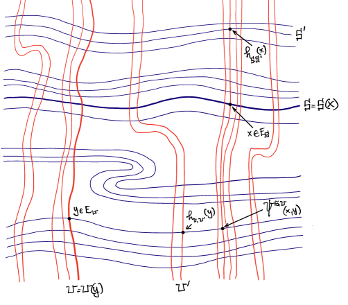
Figure 2. Illustration of Notation 2.16

The following is the key condition on tartans, which guarantees that the product measure on the set of tartan intersection points induced by the measures on the fibers agrees with the ambient measure.

Definition 2.17 (Compatible tartan).

We say that the tartan $R$ is compatible (with the ambient measure $\mu$) if, for all stable and unstable fibers ${{\mathfrak{s}}}$ and ${{\mathfrak{u}}}$, the bijection $\psi^{{{\mathfrak{s}}},{{\mathfrak{u}}}}\colon E^{{\mathfrak{s}}}\times E^{{\mathfrak{u}}}\to R^{\pitchfork}$ is bi-measurable, and $\psi^{{{\mathfrak{s}}},{{\mathfrak{u}}}}_{*}\nu_{{{\mathfrak{s}}},{{\mathfrak{u}}}}=\mu|_{R^{\pitchfork}}$.

Important consequences of compatibility, proved in [15], include:

1. The stream measures are the disintegration of the ambient measure onto fibers: if $A\subset R^{\pitchfork}$ is Borel, then

   $$\mu(A)=\int_{E^{{\mathfrak{s}}}}\nu_{{{\mathfrak{u}}}(x)}(A\cap{{\mathfrak{u}}}(x))\,d\nu_{{\mathfrak{s}}}(x)=\int_{E^{{\mathfrak{u}}}}\nu_{{{\mathfrak{s}}}(y)}(A\cap{{\mathfrak{s}}}(y))\,d\nu_{{\mathfrak{u}}}(y).$$

2. The stream measures are holonomy invariant in tartans. Let ${{\mathfrak{s}}}$ and ${{\mathfrak{s}}}^{\prime}$ be stable fibers of $R$, and $A\subset E^{{\mathfrak{s}}}$ be $\nu_{{\mathfrak{s}}}$-measurable. Then $A^{\prime}=h_{{{\mathfrak{s}}},{{\mathfrak{s}}}^{\prime}}(A)$ is $\nu_{{{\mathfrak{s}}}^{\prime}}$-measurable, and $\nu_{{{\mathfrak{s}}}^{\prime}}(A^{\prime})=\nu_{{\mathfrak{s}}}(A)$. The analogous statement holds for holonomies $h_{{{\mathfrak{u}}},{{\mathfrak{u}}}^{\prime}}$.

The final condition on the turbulations is that the compatible tartans see a full measure subset of $\Sigma$.

Definition 2.18 (Full turbulations).

We say that the transverse pair $({{\mathcal{T}}}^{s},\nu^{s})$ and $({{\mathcal{T}}}^{u},\nu^{u})$ is full if

1. There is a countable collection $R_{i}$ of (positive measure) compatible tartans with $\mu\left(\bigcup_{i}R_{i}^{\pitchfork}\right)=1$; and

2. for every non-empty open subset $U$ of $\Sigma$, there is a positive measure compatible tartan $R=(R^{s},R^{u})$ with $R^{s}\cup R^{u}\subset U$.

Part (b) of the definition is an additional regularity condition, which prevents the fibers of tartans from behaving too wildly between intersection points. In [15], a variety of conditions is presented, each of which, together with part (a) of the definition, implies part (b). Here we only state the condition which we will use later.

Definition 2.19 (Regular tartan).

We say that a tartan $R$ is regular if for all $x\in R^{\pitchfork}$ and all neighborhoods $U$ of $x$, there is some $\delta>0$ such that if $y\in{{\mathfrak{s}}}(x)\cap R^{\pitchfork}$ and $z\in{{\mathfrak{u}}}(x)\cap R^{\pitchfork}$ with $\nu_{{{\mathfrak{s}}}(x)}([x,y]_{s})<\delta$ and $\nu_{{{\mathfrak{u}}}(x)}([x,z]_{u})<\delta$, then the stream arcs $[x,y]_{s}$, $[y,{{\mathfrak{s}}}(z)\pitchfork{{\mathfrak{u}}}(y)]_{u}$, $[{{\mathfrak{s}}}(z)\pitchfork{{\mathfrak{u}}}(y),z]_{s}$, and $[z,x]_{u}$ are all contained in $U$.

Lemma 2.20.

Suppose that part (a) of Definition 2.18 is satisfied, and in addition each of the tartans $R_{i}$ is regular. Then part (b) of the definition is also satisfied.

Remark 2.21.

If a tartan $R$ is regular, then so is $F(R)$.

2.3. Measurable pseudo-Anosov maps

Definitions 2.22 (measurable pseudo-Anosov turbulations, measurable pseudo-Anosov map, dilatation).

A pair $({{\mathcal{T}}}^{s},\nu^{s}),({{\mathcal{T}}}^{u},\nu^{u})$ of measured turbulations on $\Sigma$ are said to be measurable pseudo-Anosov turbulations if they are transverse, tame, full, and have dense streamlines.

A $\mu$-preserving homeomorphism $F\colon\Sigma\to\Sigma$ is measurable pseudo-Anosov if there is a pair $({{\mathcal{T}}}^{s},\nu^{s}),({{\mathcal{T}}}^{u},\nu^{u})$ of measurable pseudo-Anosov turbulations and a number $\lambda>1$, called the dilatation of $F$, such that $F({{\mathcal{T}}}^{s},\nu^{s})=({{\mathcal{T}}}^{s},\lambda\nu^{s})$ and $F({{\mathcal{T}}}^{u},\nu^{u})=({{\mathcal{T}}}^{u},\lambda^{-1}\nu^{u})$.

In the hypotheses of the following lemma, note that we are not assuming that $F$ is a measurable pseudo-Anosov map: rather, the lemma will be used to prove that the homeomorphisms $F_{\lambda}$ are measurable pseudo-Anosov maps, by propagating a single positive measure compatible tartan over a full measure subset of $\Sigma$ using the ergodicity of $F_{\lambda}$.

Lemma 2.23.

Let $({{\mathcal{T}}}^{s},\nu^{s}),({{\mathcal{T}}}^{u},\nu^{u})$ be a transverse pair of measured turbulations on $\Sigma$, and suppose that $F\colon\Sigma\to\Sigma$ is $\mu$-preserving and satisfies $F({{\mathcal{T}}}^{s},\nu^{s})=({{\mathcal{T}}}^{s},\lambda\nu^{s})$ and $F({{\mathcal{T}}}^{u},\nu^{u})=({{\mathcal{T}}}^{u},\lambda^{-1}\nu^{u})$ for some $\lambda>1$.

If $R=(R^{s},R^{u})$ is a compatible tartan, then so is $F(R)$ (the tartan whose fibers are the $F$-images of the fibers of $R$).

Proof.

It is immediate from Definitions 2.15 that $F(R)$ is a tartan, and that $F(R)^{\pitchfork}=F(R^{\pitchfork})$.

For compatibility, let ${{\mathfrak{s}}}$ and ${{\mathfrak{u}}}$ be any stable and unstable fibers of $R$, and write ${{\mathfrak{s}}}^{\prime}$ and ${{\mathfrak{u}}}^{\prime}$ for the image fibers of $F(R)$. Then there is a commutative diagram of bijections

$$\begin{CD}E^{{\mathfrak{s}}}\times E^{{\mathfrak{u}}}@>{\psi^{{{\mathfrak{s}}},{{\mathfrak{u}}}}}>{}>R^{\pitchfork}\\ @V{}V{F\times F}V@V{}V{F}V\\ E^{{\mathfrak{s}^{\prime}}}\times E^{{\mathfrak{u}^{\prime}}}@>{\psi^{{{\mathfrak{s}^{\prime}}},{{\mathfrak{u}^{\prime}}}}}>{}>F(R)^{\pitchfork}.\end{CD}$$

The bi-measurability of $\psi^{{{\mathfrak{s}^{\prime}}},{{\mathfrak{u}^{\prime}}}}$ follows from that of $\psi^{{{\mathfrak{s}}},{{\mathfrak{u}}}}$ since $F$ and $F\times F$ are homeomorphisms. Since $F_{*}(\nu_{{\mathfrak{s}}})=\lambda\nu_{{\mathfrak{s}^{\prime}}}$ and $F_{*}(\nu_{{\mathfrak{u}}})=\lambda^{-1}\nu_{{\mathfrak{u}^{\prime}}}$, we have $(F\times F)_{*}\nu_{{{\mathfrak{s}}},{{\mathfrak{u}}}}=\nu_{{{\mathfrak{s}}}^{\prime},{{\mathfrak{u}}}^{\prime}}$, and hence $F_{*}(\psi_{*}^{{{\mathfrak{s}}},{{\mathfrak{u}}}}\nu_{{{\mathfrak{s}}},{{\mathfrak{u}}}})=\psi_{*}^{{{\mathfrak{s}^{\prime}}},{{\mathfrak{u}^{\prime}}}}\nu_{{{\mathfrak{s}^{\prime}}},{{\mathfrak{u}^{\prime}}}}$. However $\psi_{*}^{{{\mathfrak{s}}},{{\mathfrak{u}}}}\nu_{{{\mathfrak{s}}},{{\mathfrak{u}}}}=\mu|_{R^{\pitchfork}}$ by compatibility of $R$, so that $\psi_{*}^{{{\mathfrak{s}^{\prime}}},{{\mathfrak{u}^{\prime}}}}\nu_{{{\mathfrak{s}^{\prime}}},{{\mathfrak{u}^{\prime}}}}=\mu|_{F(R)^{\pitchfork}}$ by $F$-invariance of $\mu$ as required. ∎

It is immediate from the definitions that any pseudo-Anosov map is a generalized pseudo-Anosov map. We now show that any generalized pseudo-Anosov map $F\colon\Sigma\to\Sigma$ with dense non-singular leaves is a measurable pseudo-Anosov map.

Lemma 2.24.

Let $F\colon\Sigma\to\Sigma$ be generalized pseudo-Anosov, and suppose that the non-singular leaves of its invariant foliations are dense in $\Sigma$. Then $F$ is also measurable pseudo-Anosov, with the streamlines of its (un)stable invariant turbulation given by the non-singular leaves $\ell$ of the (un)stable foliation ${{\mathcal{F}}}^{s/u}$, carrying the measures $\nu_{\ell}^{s/u}$.

Proof.

The stable and unstable streamlines are obtained from the stable and unstable foliations by omitting the finitely many singleton leaves at points of $Z$, and the countably many leaves emanating from points of $Y$. These omitted leaves have zero measure by Remark 2.9, so that $({{\mathcal{T}}}^{s},\nu^{s})$ and $({{\mathcal{T}}}^{u},\nu^{u})$ cover full measure in $\Sigma$ and hence are turbulations. Clearly $F$ preserves $\mu$ and satisfies $F({{\mathcal{T}}}^{s},\nu^{s})=({{\mathcal{T}}}^{s},\lambda\nu^{s})$ and $F({{\mathcal{T}}}^{u},\nu^{u})=({{\mathcal{T}}}^{u},\lambda^{-1}\nu^{u})$. It remains therefore to show that the turbulations are measurable pseudo-Anosov turbulations (Definitions 2.22). The streamlines are dense by assumption, so it remains to show that the turbulations are transverse; that they are tame; and that they are full.

By Definition 2.6, there are regular chart domains $D_{x}$ about each point $x\in\Sigma\setminus(Y\cup Z)$ together with ambient and stream measure preserving homeomorphisms $\Phi_{x}\colon D_{x}\to M_{x}$ to regular models. In particular, the stable and unstable turbulations are transverse. For fullness, the stable and unstable leaf segments of $D_{x}$ which are not contained in singular leaves form a tartan $R_{x}=(R^{s}_{x},R^{u}_{x})$, whose compatibility with $\mu$ is immediate using $\Phi_{x}$. Moreover we have $\mu(R_{x}^{\pitchfork})=\mu(D_{x})>0$ by Remark 2.9. Since $\Sigma\setminus(Y\cup Z)$ is separable, it is covered by countably many chart domains $D_{i}=D_{x_{i}}$: the corresponding tartans $R_{i}$ provide a countable collection of compatible tartans with $\mu\left(\bigcup_{i}R_{i}^{\pitchfork}\right)=1$. The second condition in the Definition of fullness is immediate, since every non-empty open subset $U$ of $\Sigma$ contains a regular point $x$, and the chart domain $D_{x}$ can be restricted to a subset of $U$.

It remains to show that the turbulations are tame. Let $d$ be a metric on $\Sigma$ compatible with its topology, and suppose for a contradiction that there is some $\epsilon>0$ and a sequence $([x_{i},y_{i}])$ of stream arcs — of either turbulation — with measures converging to zero, such that $d(x_{i},y_{i})\geq\epsilon$ for all $i$. By taking a subsequence, we can assume that $x_{i}\to x^{*}\in\Sigma$ and $y_{i}\to y^{*}\in\Sigma$.

Consider first the case $x^{*}\not\in Z$, so that there is a chart domain $D$ about $x^{*}$ and an ambient and stream-measure preserving homeomorphism $\Phi\colon D\to R$ or $\Phi\colon D\to Q$ to a regular or pronged model. Let $\eta>0$ be such that the leaf through $x^{*}$ has segments of measure $\eta$ on each side of $x^{*}$ contained in $D$ (or on each prong emanating from $x^{*}$ if $x^{*}\in Y$). For $i$ sufficiently large, we have that $x_{i}\in D$, and the streamline through $x_{i}$ has measure at least $\eta/2$ on each side of $x_{i}$ contained in $D$. Since the measure of $[x_{i},y_{i}]$ converges to $0$, we have $[x_{i},y_{i}]\subset D$ for sufficiently large $i$. Then $\Phi([x_{i},y_{i}])$ is a horizontal or vertical segment with Lebesgue measure converging to zero, so that $\Phi(y_{i})\to\Phi(x^{*})$, and hence $y_{i}\to x^{*}$, contradicting $d(x_{i},y_{i})\geq\epsilon$.

Therefore we must have $x^{*}\in Z$ and, analogously, $y^{*}\in Z$. We obtain the required contradiction by showing that there is a positive lower bound on the measure of any stream arc which connects sufficiently small neighborhoods of two distinct points of $Z$.

Pick $\xi>0$ such that distinct elements $z_{1},z_{2}$ of $Z$ have $d(z_{1},z_{2})>5\xi$. Let $U=\bigcup_{z\in Z}B(z,\xi)$, a union of $|Z|$ disjoint open disks. Cover $\Sigma\setminus U$ with a finite collection $(D_{i})$ of (regular or pronged) chart domains of diameter less than $\xi$. Any stream arc with endpoints in different components of $U$ must intersect some $D_{i}$ which is contained entirely in $\Sigma\setminus U$, and therefore must contain an entire leaf segment (or perhaps two prongs of an $n$-od leaf segment in the pronged case). However, in each chart domain there is a minimum measure of such leaf segments (coming from the models of Definitions 2.2 and 2.3). The required lower bound on the stream measure of any stream arc which connects two different components of $U$ follows.

∎

3. Background

In this section we review the material which forms the background of this work, and state some key results from old and recent papers. Section 3.1 concerns tent maps and their study using symbolic dynamics. In Section 3.2 we discuss inverse limits of tent maps. Finally, in Section 3.3, we summarize key properties of the absolutely continuous invariant measures of tent maps, and state some results from [13] which will play a key rôle in this paper.

3.1. Tent maps

Definition 3.1 (Tent map, see Figure 3).

Let $\lambda\in(\sqrt{2},2)$. The (core) tent map $f_{\lambda}\colon[a_{\lambda},b_{\lambda}]\to[a_{\lambda},b_{\lambda}]$ of slope $\lambda$ is the restriction of the map $T_{\lambda}\colon[0,1]\to[0,1]$ defined by $T_{\lambda}(x)=\min(\lambda x,\lambda(1-x))$ to the interval $I_{\lambda}:=[a_{\lambda},b_{\lambda}]:=[T_{\lambda}^{2}(1/2),T_{\lambda}(1/2)]$. We write $c=1/2$, the turning point of $f_{\lambda}$.

Throughout the paper we work with a single tent map of fixed slope and drop the subscripts $\lambda$, writing simply $f\colon I\to I$, where $I=[a,b]$.

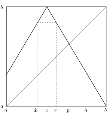
Figure 3. A tent map $f\colon I\to I$

Notation 3.2 (PC).

The post-critical set is denoted ${\text{PC}}:=\{f^{r}(c)\,:\,r\geq 1\}$.

Notice that $f(c)=b$ and $f(b)=a$, so that $a,b\in{\text{PC}}$.

Notation 3.3 (${{\hat{x}}}$, see Figure 3).

Let ${{\hat{a}}}\in[c,b]$ satisfy $f({{\hat{a}}})=f(a)$. For each $x\in[a,{{\hat{a}}}]$ with $x\not=c$, we write ${{\hat{x}}}$ for the unique element of $I$ with ${{\hat{x}}}\not=x$ and $f({{\hat{x}}})=f(x)$.

The fundamental idea of the symbolic approach to the dynamics of tent maps is to code orbits of $f$ with sequences of $0$s and $1$s, according as successive points along the orbit lie to the left or to the right of the turning point. This leaves open the question of which symbol to use when the orbit passes through the turning point. We take a hybrid approach, leaving the choice open when the turning point is not periodic, and making a choice based on the parity of the orbit of the turning point when it is periodic. This approach has the advantage of giving clean necessary and sufficient admissibility conditions for a sequence to be an itinerary [12].

Definition 3.4 (Itinerary $j(x)$, kneading sequence $\kappa(f)$).

If $c$ is a periodic point of $f$, of period $n$, write $\varepsilon(f)=0$ (respectively $\varepsilon(f)=1$) if an even (respectively odd) number of the points $\{f^{r}(c)\,:\,1\leq r<n\}$ lie in $(c,b]$. The itinerary $j(x)\in{\{0,1\}^{{\mathbb{N}}}}$ of a point $x\in I$ is then defined by

$$j(x)_{r}=\begin{cases}0&\text{ if }f^{r}(x)\in[a,c),\\ 1&\text{ if }f^{r}(x)\in(c,b],\\ \varepsilon(f)&\text{ if }f^{r}(x)=c\end{cases}\qquad\text{ for each }r\in{{\mathbb{N}}}$$

(we adopt the convention that $0\in{{\mathbb{N}}}$).

If $c$ is not a periodic point of $f$, we say that a sequence $s\in{\{0,1\}^{{\mathbb{N}}}}$ is an itinerary of $x\in I$ if $f^{r}(x)\in[a,c]$ whenever $s_{r}=0$, and $f^{r}(x)\in[c,b]$ whenever $s_{r}=1$. Therefore each $x\in I$ has exactly two itineraries if $c\in\operatorname{orb}(x,f):=\{f^{r}(x)\,:\,r\in{{\mathbb{N}}}\}$, and a unique itinerary otherwise.

With an abuse of notation, we write $j(x)=s$ to mean that $s$ is an itinerary of $x$. With this abusive notation we have that $j(x)=s\implies j(f(x))=\sigma(s)$, where $\sigma\colon\{0,1\}^{{\mathbb{N}}}\to\{0,1\}^{{\mathbb{N}}}$ is the shift map.

Since $f$ is uniformly expanding on each of its branches, any sequence $s\in\{0,1\}^{{\mathbb{N}}}$ is the itinerary of at most one point $x\in I$.

The kneading sequence $\kappa(f)\in{\{0,1\}^{{\mathbb{N}}}}$ of $f$ is defined to be the itinerary of $b$ (which is well defined, since if $c$ is not a periodic point then $c\not\in\operatorname{orb}(b,f)$).

Definition 3.5 (Unimodal order).

The unimodal order (also known as the parity-lexicographical order) is a total order $\preceq$ on ${\{0,1\}^{{\mathbb{N}}}}$, defined as follows: if $s$ and $t$ are distinct elements of ${\{0,1\}^{{\mathbb{N}}}}$, let $r\in{{\mathbb{N}}}$ be least such that $s_{r}\not=t_{r}$. Then $s\preceq t$ if and only if $\sum_{i=0}^{r}s_{i}$ is even.

Remark 3.6.

The unimodal order is defined precisely to reflect the usual order of points on the interval: if $s$ and $t$ are itineraries of $x$ and $y$, then $x<y\implies s\prec t$; and, conversely, if $s\prec t$ then either $x<y$, or $s$ and $t$ are the two itineraries of $x=y$ in the case where $c$ is not periodic.

Remark 3.7.

As in Definition 3.1, we only consider tent maps $f$ whose slope $\lambda$ satisfies $\sqrt{2}<\lambda<2$, that is, whose topological entropy $h(f)=\log\lambda$ satisfies $\frac{\log 2}{2}<h(f)<\log 2$. The condition $\lambda>\sqrt{2}$ is equivalent to each of the following:

• $f$ is not renormalizable;

• $\kappa(f)\succ 10(11)^{\infty}$;

• $\kappa(f)=10(11)^{k}0\dots$ for some $k\geq 0$.

It is also equivalent (see Theorem 4.7) to the statement that $q(f)<1/2$, where $q(f)$ is the height of $f$ as given by Definition 4.6.

The condition $\lambda<2$ is to avoid cluttering statements with exceptions for the special case $\lambda=2$ (in which the natural extension of $f$ is semi-conjugate to a generalized pseudo-Anosov map called the tight horseshoe map, see for example [22]).

The following lemma is dependent on the assumption that $\lambda>\sqrt{2}$.

Lemma 3.8.

$f(a)<p<{{\hat{a}}}$, where $p$ is the fixed point of $f$ (see Figure 3).

Proof.

By Remark 3.7 we have $j(a)=0(11)^{k}0\dots$ for some $k\geq 0$, so that $j({{\hat{a}}})=1(11)^{k}0\dots$ and $j(f(a))=(11)^{k}0\dots$. Comparing these itineraries in the unimodal order with $j(p)=1^{\infty}$ and using Remark 3.6 gives the result. ∎

3.2. Inverse limits

Inverse limits of tent maps have been intensively studied, both for their intrinsic interest as complicated topological spaces, and in dynamical systems as models for attractors [2, 4, 5, 7, 11, 16, 20, 32].

Definitions 3.9 (Inverse limit ${{\widehat{I}}}$, projections $\pi_{r}$, natural extension ${{\widehat{f}}}$).

The inverse limit ${{\widehat{I}}}={{\widehat{I}}}_{\lambda}$ of the tent map $f\colon I\to I$ is the space

$${{\widehat{I}}}=\{{{\mathbf{x}}}\in I^{{\mathbb{N}}}\,:\,f(x_{r+1})=x_{r}\text{ for all }r\in{{\mathbb{N}}}\}\subset I^{{\mathbb{N}}},$$

endowed with the metric $d({{\mathbf{x}}},{{\mathbf{y}}})=\sum_{r=0}^{\infty}|x_{r}-y_{r}|/2^{r}$, which induces its natural topology as a subset of the product space $I^{{\mathbb{N}}}$.

We denote elements of ${{\widehat{I}}}$ with angle brackets, ${{\mathbf{x}}}=\left<x_{0},x_{1},x_{2},\dots\right>$.

For each $r\in{{\mathbb{N}}}$, we denote by $\pi_{r}\colon{{\widehat{I}}}\to I$ the projection onto the $r^{\text{th}}$ coordinate, $\pi_{r}({{\mathbf{x}}})=x_{r}$.

The natural extension of $f$ is the homeomorphism ${{\widehat{f}}}\colon{{\widehat{I}}}\to{{\widehat{I}}}$ defined by

$${{\widehat{f}}}(\left<x_{0},x_{1},x_{2},\dots\right>)=\left<f(x_{0}),x_{0},x_{1},x_{2},\dots\right>.$$

Clearly each $\pi_{r}$ is a semi-conjugacy from ${{\widehat{f}}}\colon{{\widehat{I}}}\to{{\widehat{I}}}$ to $f\colon I\to I$. It is straightforward to see that any semi-conjugacy from a homeomorphism $F\colon X\to X$ to $f$ factors through each $\pi_{r}$.

Since $\pi_{r}=\pi_{0}\circ{{\widehat{f}}}^{-r}$, we have that, for all ${{\mathbf{x}}}\in{{\widehat{I}}}$,

$${{\mathbf{x}}}=\left<\pi_{0}({{\mathbf{x}}}),\pi_{0}({{\widehat{f}}}^{-1}({{\mathbf{x}}})),\pi_{0}({{\widehat{f}}}^{-2}({{\mathbf{x}}})),\dots\right>.$$ (1)

The next result is an important consequence of the condition that $\lambda\in(\sqrt{2},2)$.

Lemma 3.10.

For every ${{\mathbf{x}}}\in{{\widehat{I}}}$, there are infinitely many $r\in{{\mathbb{N}}}$ with $x_{r}\in[f(a),b)$: that is, infinitely many $r\in{{\mathbb{N}}}$ such that $x_{r}$ has two preimages.

Proof.

Let $p>c$ be the fixed point of $f$. If $x_{r}\leq p$ then $x_{r+1}$, being a preimage of $x_{r}$, satisfies either $x_{r+1}<c$ or $x_{r+1}\geq p$ (see Figure 3). Since $\lambda<2$, there is an upper bound on the number of consecutive entries of ${{\mathbf{x}}}$ which are smaller than $c$: hence $x_{r}\geq p$ for infinitely many $r\in{{\mathbb{N}}}$.

Since $p>f(a)$ by Lemma 3.8, there are infinitely many $r$ with $x_{r}\in(f(a),b]$. However if $x_{r}=b$ for some $r\geq 2$ then $x_{r-2}=f(a)$, and the result follows. ∎

Definitions 3.11 ($\pi_{0}$-fibers $\left[x\right]$, cylinder sets $[x,y_{1},\dots,y_{r}]$).

For each $x\in I$ we define the $\pi_{0}$-fiber $\left[x\right]$ of ${{\widehat{I}}}$ above $x$ by $\left[x\right]=\pi_{0}^{-1}(x)$.

More generally, if $f(y_{1})=x$ and $f(y_{i})=y_{i-1}$ for $2\leq i\leq r$, we define the cylinder set $\left[x,y_{1},\dots,y_{r}\right]\subset\left[x\right]$ by

$$\left[x,y_{1},\dots,y_{r}\right]=\{{{\mathbf{x}}}\in\left[x\right]\,:\,x_{i}=y_{i}\text{ for }1\leq i\leq r\}.$$

Note that the diameter of $\left[x,y_{1},\dots,y_{r}\right]$ is bounded above by $1/2^{r}$, so that the cylinder subsets of $\left[x\right]$ form a basis for its topology.

Definition 3.12 (Arc).

An (open, half-open, or closed) arc in ${{\widehat{I}}}$ is a subset of ${{\widehat{I}}}$ which is a continuous injective image of an (open, half-open, or closed) interval.

An open arc in ${{\widehat{I}}}$ is therefore synonymous with an immersed line in ${{\widehat{I}}}$ (Definition 2.10).

We will need the following well-known facts about the topology of ${{\widehat{I}}}$ (the former is theorem 2.2 of [32], the latter is folklore).

Lemma 3.13.

1. If ${{\mathbf{x}}}\in{{\widehat{I}}}$ is not in the $\omega$-limit set $\omega(\left[c\right],{{\widehat{f}}})$ of the critical fiber, then it has a neighborhood homeomorphic to the product of an open interval and a Cantor set.

2. Every path component of ${{\widehat{I}}}$ is either a point or an arc.

It is worth noting how badly Lemma 3.13(a) can fail for points in the $\omega$-limit set of the critical fiber. Barge, Brucks, and Diamond [4] show that there is a dense $G_{\delta}$ set of parameters $\lambda$ for which every open subset of ${{\widehat{I}}}_{\lambda}$ contains a homeomorphic copy of ${{\widehat{I}}}_{\lambda^{\prime}}$ for every $\lambda^{\prime}\in(\sqrt{2},2)$.

Nevertheless, the fibers of tent maps inverse limits are regular (in the case $\lambda>\sqrt{2}$).

Lemma 3.14.

$\left[x\right]$ is a Cantor set for all $x\in I$.

Proof.

$\left[x\right]$ is certainly compact and totally disconnected. To see that it is perfect, let ${{\mathbf{x}}}\in\left[x\right]$ and $R>0$. By Lemma 3.10 there is some $r>R$ for which $x_{r}$ has two preimages $x_{r+1}$ and ${{\hat{x}}}_{r+1}$. Let ${{\mathbf{x}}}^{\prime}\in\left[x\right]$ have $x^{\prime}_{i}=x_{i}$ for $i\leq r$ and $x^{\prime}_{r+1}={{\hat{x}}}_{r+1}$. Then $0<d({{\mathbf{x}}},{{\mathbf{x}}}^{\prime})<1/2^{R}$. ∎

We can introduce symbolic dynamics on ${{\widehat{I}}}$ just as we did for forwards orbits of tent maps.

Definition 3.15 (Itineraries on ${{\widehat{I}}}$).

Let ${{\mathbf{x}}}\in{{\widehat{I}}}$. An element $s$ of ${\{0,1\}^{{\mathbb{N}}}}$ is said to be an itinerary of ${{\mathbf{x}}}$ if $s_{r}=0\implies x_{r+1}\leq c$, and $s_{r}=1\implies x_{r+1}\geq c$. In an abuse of notation, we write $J({{\mathbf{x}}})=s$ to mean that $s$ is an itinerary of ${{\mathbf{x}}}$.

Remark 3.16.

1. An element ${{\mathbf{x}}}$ of $\left[x\right]$ is determined by its itinerary $J({{\mathbf{x}}})=s$, since the $x_{r}$ are determined inductively by $x_{0}=x$; and $x_{r+1}$ is the unique preimage of $x_{r}$ which lies in $[a,c]$ if $s_{r}=0$, or in $[c,b]$ if $s_{r}=1$.

2. If $x\not\in{\text{PC}}$, then every element of $\left[x\right]$ has a unique itinerary, and if $c$ is not a periodic point of $f$ then every element of ${{\widehat{I}}}$ has at most two itineraries. More generally, for any ${{\mathbf{x}}}\in{{\widehat{I}}}$, the set of itineraries of ${{\mathbf{x}}}$ is closed in ${\{0,1\}^{{\mathbb{N}}}}$.

By Remark 3.16(b), if $x\not\in{\text{PC}}$ then the fiber $\left[x\right]$ can be totally ordered by the unimodal order on the itineraries of its elements. In particular, this makes it possible to define consecutive elements of the fiber.

Definition 3.17 (Consecutive elements of $\left[x\right]$).

Let $x\not\in{\text{PC}}$, so that every ${{\mathbf{x}}}\in\left[x\right]$ has a unique itinerary $J({{\mathbf{x}}})$. We say that distinct points ${{\mathbf{x}}},{{\mathbf{x}}}^{\prime}\in\left[x\right]$ are consecutive if there is no point of $\left[x\right]$ whose itinerary lies strictly between $J({{\mathbf{x}}})$ and $J({{\mathbf{x}}}^{\prime})$ in the unimodal order.

More generally, we can consider all of the itineraries which are realized in a fiber.

Definition 3.18 (${{\mathcal{K}}}_{x}$, $L_{x}\colon{{\mathcal{K}}}_{x}\to\left[x\right]$).

For each $x\in I$, write

$${{\mathcal{K}}}_{x}=\{s\in{\{0,1\}^{{\mathbb{N}}}}\,:\,s\text{ is an itinerary of some ${{\mathbf{x}}}\in\left[x\right]$}\}.$$

By Remark 3.16(a), there is a function $L_{x}\colon{{\mathcal{K}}}_{x}\to\left[x\right]$ defined by $L_{x}(J({{\mathbf{x}}}))={{\mathbf{x}}}$ for all ${{\mathbf{x}}}\in\left[x\right]$.

Lemma 3.19.

For each $x\in I$, ${{\mathcal{K}}}_{x}$ is compact and $L_{x}\colon{{\mathcal{K}}}_{x}\to\left[x\right]$ is continuous.

More generally, if ${{\mathcal{V}}}=\{(x,s)\in I\times\{0,1\}^{{\mathbb{N}}}\,:\,s\in{{\mathcal{K}}}_{x}\}$, then the function $L\colon{{\mathcal{V}}}\to{{\widehat{I}}}$ defined by $L(x,s)=L_{x}(s)$ is continuous.

Proof.

Compactness of ${{\mathcal{K}}}_{x}$ is straightforward: if $s^{(i)}\to s$ are itineraries of ${{\mathbf{x}}}^{(i)}\in\left[x\right]$ with ${{\mathbf{x}}}^{(i)}\to{{\mathbf{x}}}$, then $s$ is an itinerary of ${{\mathbf{x}}}$.

For continuity of $L_{x}$, note that if ${{\mathbf{x}}},{{\mathbf{y}}}\in\left[x\right]$ and $J({{\mathbf{x}}})_{r}=J({{\mathbf{y}}})_{r}$ for all $r\leq R$, then $x_{r}=y_{r}$ for all $r\leq R$.

For the final statement, note that if ${{\mathbf{x}}},{{\mathbf{y}}}\in{{\widehat{I}}}$ with $|x_{0}-y_{0}|<\epsilon$ and $J({{\mathbf{x}}})_{r}=J({{\mathbf{y}}})_{r}$ for all $r\leq R$, then $|x_{r}-y_{r}|<\epsilon/\lambda^{r}$ for all $r\leq R$. ∎

Remark 3.20.

It follows that if $x\not\in{\text{PC}}$, so that $J|_{\left[x\right]}\colon\left[x\right]\to{{\mathcal{K}}}_{x}$ is well-defined, then this map is continuous, being the inverse of the continuous bijection $L_{x}$.

3.3. Invariant measures

Recall (for example [3, 18, 24, 26, 27, 28, 33]) that each tent map $f=f_{\lambda}$ has a unique invariant Borel probability measure $\mu=\mu_{\lambda}$ which is absolutely continuous with respect to Lebesgue measure $m$, and $d\mu=\varphi\,dm$, for some $\varphi\in L^{1}(m)$ defined on $[a,b]\setminus{\text{PC}}$ which is bounded away from zero, of bounded variation, and satisfies, for all $x\not\in{\text{PC}}$ and $r\in{{\mathbb{N}}}$,

$$\varphi(x)=\sum_{f^{r}(y)=x}\frac{\varphi(y)}{\lambda^{r}}$$ (2)

Moreover, $\mu$ is ergodic.

This measure $\mu$ induces an ergodic ${{\widehat{f}}}$-invariant OU probability measure ${{\hat{\mu}}}$ on ${{\widehat{I}}}$ characterized by $(\pi_{r})_{*}({{\hat{\mu}}})=\mu$ for all $r\in{{\mathbb{N}}}$ [31].

The following result is from [13].

Lemma 3.21.

For each $x\not\in{\text{PC}}$, there is a Borel measure $\alpha_{x}$ on ${{\widehat{I}}}$, which is supported on $\left[x\right]$ and is given on cylinder subsets of $\left[x\right]$ by

$$\alpha_{x}(\left[x,y_{1},\dots,y_{r}\right])=\frac{\varphi(y_{r})}{\lambda^{r}}.$$

In particular, $\alpha_{x}(\left[x\right])=\varphi(x)$.

Remarks 3.22.

1. $\alpha_{x}$ is OU: since the cylinder subsets form a basis of $\left[x\right]$, $\alpha_{x}$ is positive on non-empty open subsets of $\left[x\right]$; and since any point ${{\mathbf{x}}}$ is contained in $\left[x_{0},\dots,x_{r}\right]$ for all $r$, $\alpha_{x}$ is non-atomic.

2. Since ${{\widehat{f}}}(\left[x,y_{1},\dots,y_{r}\right])=\left[f(x),x,y_{1},\dots,y_{r}\right]$, we have $\alpha_{f(x)}({{\widehat{f}}}(A))=\lambda^{-1}\alpha_{x}(A)$ for every Borel subset $A$ of $\left[x\right]$.

3. If $c$ is not pre-periodic, then $\varphi$ can be extended inductively over PC by

   $$\varphi(f^{i}(c))=\sum_{f(y)=f^{i}(c)}\frac{\varphi(y)}{\lambda},$$

   so that it satisfies equation (2) for all $x\in I$; and therefore the measures $\alpha_{x}$ can be defined for all $x\in I$ in such a way that they satisfy (a) and (b).

Remarks 3.22(b) says that ${{\widehat{f}}}$ contracts $\pi_{0}$-fibers uniformly by a factor $\lambda$, with respect to the measures $\alpha_{x}$.

The images of these fibers under the semi-conjugacy $g\colon{{\widehat{I}}}\to\Sigma=S^{2}$ — which are almost all arcs — will form the stable foliation or turbulation of the generalized or measurable pseudo-Anosov map semi-conjugate to ${{\widehat{f}}}$, with the measure on leaves/streamlines coming from the $\alpha_{x}$. The unstable foliation/turbulation will come from the path components of ${{\widehat{I}}}$, together with Lebesgue measure $m$ on their $\pi_{0}$-images, which is expanded by ${{\widehat{f}}}$ by a factor $\lambda$.

The remaining definitions and results in this section are from [13]: Theorem 3.26 is lemma 8.3, Theorem 3.27 is theorem 7.1, Theorem 3.28 is theorem 8.1, Theorem 3.30 is theorem 1.1(a), and Lemma 3.31 is lemma 3.5. The reader may find it helpful to interpret these in light of the genesis of the invariant turbulations just described. The $0$-boxes of Definition 3.25 will provide the unstable fibers of a tartan, whose stable fibers come from the $\pi_{0}$-fibers of ${{\widehat{I}}}$; Theorem 3.26 will provide a tartan $R$ with $\mu(R^{\pitchfork})>0$, which will enable us to show fullness of the turbulations; Theorem 3.27 translates to unstable holonomy invariance of these tartans (stable holonomy invariance is straightforward); Theorem 3.28 will be used to show that they are compatible with $\mu$; and Theorem 3.30, together with Lemma 3.31, ensures that an unstable turbulation can be built from well-behaved path components.

Definition 3.23 ($0$-flat arc).

An arc $\Gamma$ in ${{\widehat{I}}}$ is $0$-flat (over the subinterval $J$ of $I$) if $\pi_{0}$ is injective on $\Gamma$ (and maps it onto $J$).

Remark 3.24.

Alternatively, the arc $\Gamma$ is $0$-flat if and only if $c\not\in\operatorname{Int}(\pi_{r}(\Gamma))$ for all $r\geq 1$. In particular, the points of a $0$-flat arc all share a common itinerary.

Definition 3.25 ($0$-box).

Let $J$ be a subinterval of $I$. A $0$-box $B$ over $J$ is a Borel disjoint union of $0$-flat arcs over $J$.

Theorem 3.26.

There exists a $0$-box $B$ with ${{\hat{\mu}}}(B)>0$.

Theorem 3.27 (Holonomy invariance).

Let $B$ be a $0$-box over a subinterval $J$. Then

$$\alpha_{x}(B)=\alpha_{y}(B)\quad\text{ for all $x,y\in J\setminus{\text{PC}}$}.$$

Theorem 3.28.

For every Borel subset $E$ of ${{\widehat{I}}}$, we have

$${{\hat{\mu}}}(E)=\int_{I}\alpha_{x}(E)dm(x).$$

Definition 3.29 (Globally leaf regular).

A point ${{\mathbf{x}}}\in{{\widehat{I}}}$ is said to be globally leaf regular if its path component $\Gamma$ is an open arc, and each component of $\Gamma\setminus\{{{\mathbf{x}}}\}$ is dense in ${{\widehat{I}}}$.

Theorem 3.30 (Typical path components).

${{\hat{\mu}}}$-almost every point of ${{\widehat{I}}}$ is globally leaf regular.

Globally leaf regular path components (or, more generally, open arcs) can be decomposed into $0$-flat arcs.

Lemma 3.31 ($0$-flat decomposition of globally leaf regular component).

Let $\Gamma\subset{{\widehat{I}}}$ be an open arc. Then there is a countable (finite, infinite, or bi-infinite) sequence $(\Gamma_{i})$ of $0$-flat arcs in ${{\widehat{I}}}$, unique up to re-indexing by an order-preserving or order-reversing bijection, such that

1. $\Gamma=\bigcup_{i}\Gamma_{i}$

2. Each $\Gamma_{i}$ is disjoint from all other $\Gamma_{j}$, except that it intersects $\Gamma_{i-1}$ and $\Gamma_{i+1}$, if they exist, at its endpoints.

3. ${{\mathbf{x}}}\in\Gamma$ is an endpoint of some $\Gamma_{i}$ if and only if $x_{r}=c$ for some $r$.

Remark 3.32.

It follows from Lemma 3.31 and Theorem 3.28 that if $\Gamma$ is the path component of a globally leaf regular point, then ${{\hat{\mu}}}(\Gamma)=0$. This is because each $\Gamma_{i}$ of Lemma 3.31 intersects each $\pi_{0}$-fiber in at most one point, so that $\alpha_{x}(\Gamma_{i})=0$ for all $x$.

4. Extreme elements of $\pi_{0}$-fibers and the outside map

If $x\not\in{\text{PC}}$ then every element of $\left[x\right]$ has a well-defined itinerary, so that $\left[x\right]$ can be totally ordered by the unimodal order and, being compact, has minimum and maximum elements. When $x\in{\text{PC}}$ there is no such order on the fiber, but there are nevertheless minimum and maximum elements of ${{\mathcal{K}}}_{x}$, the set of itineraries realized on $\left[x\right]$ (recall Definition 3.18), which correspond to unique ‘minimum’ and ‘maximum’ elements of the fiber itself. When $x=a$ or $x=b$, it turns out that these elements coincide.

These extreme elements of fibers are important because the identifications induced by the map $g\colon{{\widehat{I}}}\to\Sigma$ which semi-conjugates ${{\widehat{f}}}$ to the sphere homeomorphism $F\colon\Sigma\to\Sigma$ take place along their orbits (the identifications will be described in Lemma 5.4). In this section we study the action of ${{\widehat{f}}}$ on extreme elements, which we model with a circle map called the outside map associated to $f$. The construction [14] of the sphere homeomorphism $F\colon\Sigma\to\Sigma$ depends crucially on the dynamics of this circle map, and in particular on its rotation number, which is called the height $q(f)$ of $f$.

4.1. Extreme elements

Recall (Definition 3.18) that

$${{\mathcal{K}}}_{x}=\{s\in{\{0,1\}^{{\mathbb{N}}}}\,:\,s\text{ is an itinerary of some ${{\mathbf{x}}}\in\left[x\right]$}\}$$

for each $x\in I$, and that $L_{x}\colon{{\mathcal{K}}}_{x}\to\left[x\right]$ associates to each $s\in{{\mathcal{K}}}_{x}$ the unique ${{\mathbf{x}}}\in\left[x\right]$ with that itinerary. Since ${{\mathcal{K}}}_{x}$ is compact (Lemma 3.19) and every non-empty subset of ${\{0,1\}^{{\mathbb{N}}}}$ has an infimum and supremum, ${{\mathcal{K}}}_{x}$ has a maximum element ${{\mathcal{U}}}_{x}$ and a minimum element ${{\mathcal{L}}}_{x}$ with respect to the unimodal order.

Definition 4.1 (Upper, lower, extreme elements, ${{\mathbf{e}}}(x_{u})$, ${{\mathbf{e}}}(x_{\ell})$).

For each $x\in I$, we write ${{\mathbf{e}}}(x_{u})=L_{x}({{\mathcal{U}}}_{x})$ and ${{\mathbf{e}}}(x_{\ell})=L_{x}({{\mathcal{L}}}_{x})$ for the upper and lower elements of $\left[x\right]$, having as itineraries ${{\mathcal{U}}}_{x}$ and ${{\mathcal{L}}}_{x}$ respectively, and refer to them both as extreme elements. (The apparently idiosyncratic notation will become more natural in Section 4.2, where a map ${{\mathbf{e}}}$ onto the set of extreme elements will be defined.)

The following lemma describes the action of ${{\widehat{f}}}$ on extreme elements.

Lemma 4.2.

Let $x\in I$.

1. If $x<f(a)$, so that $x$ has a unique $f$-preimage $x^{1}>c$, then

   $${{\mathbf{e}}}(x_{\ell})={{\widehat{f}}}({{\mathbf{e}}}(x^{1}_{u}))\quad\text{and}\quad{{\mathbf{e}}}(x_{u})={{\widehat{f}}}({{\mathbf{e}}}(x^{1}_{\ell})).$$

2. If $f(a)\leq x<b$, so that $x$ has preimages $x^{0}<c$ and $x^{1}>c$, then

   $${{\mathbf{e}}}(x_{\ell})={{\widehat{f}}}({{\mathbf{e}}}(x^{0}_{\ell}))\quad\text{and}\quad{{\mathbf{e}}}(x_{u})={{\widehat{f}}}({{\mathbf{e}}}(x^{1}_{\ell})).$$

3. If $x=b$, so that $x$ has unique preimage $c$, then

   $${{\mathbf{e}}}(b_{\ell})={{\mathbf{e}}}(b_{u})={{\widehat{f}}}({{\mathbf{e}}}(c_{\ell})).$$

Proof.

1. We have $\left[x\right]={{\widehat{f}}}(\left[x^{1}\right])$; and if ${{\mathbf{x}}}\in\left[x^{1}\right]$, then the itineraries of ${{\widehat{f}}}({{\mathbf{x}}})\in\left[x\right]$ are exactly the itineraries of ${{\mathbf{x}}}$ with a symbol $1$ prepended, so that ${{\widehat{f}}}|_{\left[x^{1}\right]}$ reverses the order on itineraries.

2. We have $\left[x\right]={{\widehat{f}}}(\left[x^{0}\right])\sqcup{{\widehat{f}}}(\left[x^{1}\right])$; if ${{\mathbf{x}}}\in\left[x^{0}\right]$ (respectively ${{\mathbf{x}}}\in\left[x^{1}\right]$) then the itineraries of ${{\widehat{f}}}({{\mathbf{x}}})\in\left[x\right]$ are exactly those of ${{\mathbf{x}}}$ with a symbol $0$ (respectively $1$) prepended. Therefore ${{\widehat{f}}}|_{\left[x^{0}\right]}$ preserves the order on itineraries and ${{\widehat{f}}}|_{\left[x^{1}\right]}$ reverses it; and all elements of ${{\widehat{f}}}(\left[x^{1}\right])$ have larger itineraries than all elements of ${{\widehat{f}}}(\left[x^{0}\right])$.

3. We have $\left[b\right]={{\widehat{f}}}(\left[c\right])$; and if ${{\mathbf{x}}}\in\left[c\right]$, then for each itinerary of ${{\mathbf{x}}}$ there are two itineraries of ${{\widehat{f}}}({{\mathbf{x}}})\in\left[b\right]$, one with the symbol $0$ prepended and one with the symbol $1$ prepended.

∎

Recall from Definition 3.17 that, provided $x\not\in{\text{PC}}$, we can define the notion of consecutive elements of $\left[x\right]$. These will play an important rôle in the theory, since typically two elements of a fiber are identified by the semi-conjugacy $g\colon{{\widehat{I}}}\to\Sigma$ if and only if they are consecutive. The proof of Lemma 4.2 also elucidates the action of ${{\widehat{f}}}$ on pairs of consecutive points, as described by the next lemma.

Lemma 4.3.

Let $x\in I\setminus{\text{PC}}$.

1. Let $r>0$ and suppose that $f^{r}(x)\not\in{\text{PC}}$. If ${{\mathbf{x}}}$ and ${{\mathbf{x}}}^{\prime}$ are consecutive in $\left[x\right]$, then ${{\widehat{f}}}^{r}({{\mathbf{x}}})$ and ${{\widehat{f}}}^{r}({{\mathbf{x}}}^{\prime})$ are consecutive in $\left[f^{r}(x)\right]$.

2. If ${{\mathbf{x}}}$ and ${{\mathbf{x}}}^{\prime}$ are consecutive in $\left[x\right]$ and $x_{1}=x^{\prime}_{1}$, then ${{\widehat{f}}}^{-1}({{\mathbf{x}}})$ and ${{\widehat{f}}}^{-1}({{\mathbf{x}}}^{\prime})$ are consecutive in $\left[x_{1}\right]$.

3. If ${{\mathbf{x}}}$ and ${{\mathbf{x}}}^{\prime}$ are consecutive in $\left[x\right]$ and $x_{1}\not=x^{\prime}_{1}$, then ${{\widehat{f}}}^{-1}({{\mathbf{x}}})={{\mathbf{e}}}(x_{1,u})$ and ${{\widehat{f}}}^{-1}({{\mathbf{x}}}^{\prime})={{\mathbf{e}}}(x^{\prime}_{1,u})$.

4. If $x\in[a,{{\hat{a}}}]\setminus\{c\}$, then ${{\widehat{f}}}({{\mathbf{e}}}(x_{u}))$ and ${{\widehat{f}}}({{\mathbf{e}}}({{\hat{x}}}_{u}))$ are consecutive in $\left[f(x)\right]$.

The extreme elements of a fiber $\left[x\right]$ coincide if and only if $x$ is an endpoint of $I$:

Lemma 4.4.

${{\mathbf{e}}}(a_{\ell})={{\mathbf{e}}}(a_{u})$, and ${{\mathbf{e}}}(b_{\ell})={{\mathbf{e}}}(b_{u})$. On the other hand, if $x\in I\setminus\{a,b\}$ then ${{\mathbf{e}}}(x_{\ell})\not={{\mathbf{e}}}(x_{u})$.

Proof.

${{\mathbf{e}}}(b_{\ell})={{\mathbf{e}}}(b_{u})$ by Lemma 4.2(c), and it follows from Lemma 4.2(a) that ${{\mathbf{e}}}(a_{\ell})={{\mathbf{e}}}(a_{u})={{\widehat{f}}}({{\mathbf{e}}}(b_{u})={{\mathbf{e}}}(b_{\ell}))$.

Suppose then that $x\in(a,b)$. By Lemma 3.10, there is some $y\in[f(a),b)$ and $r\in{{\mathbb{N}}}$ such that $f^{r}(y)=x$ and $f^{i}(y)\in(a,f(a))$ for $1\leq i<r$. Then ${{\mathbf{e}}}(y_{\ell})\not={{\mathbf{e}}}(y_{u})$ by Lemma 4.2(b); and $\{{{\mathbf{e}}}(x_{\ell}),{{\mathbf{e}}}(x_{u})\}=\{{{\widehat{f}}}^{r}({{\mathbf{e}}}(y_{\ell})),{{\widehat{f}}}^{r}({{\mathbf{e}}}(y_{u}))\}$ by Lemma 4.2(a), so that ${{\mathbf{e}}}(x_{\ell})\not={{\mathbf{e}}}(x_{u})$ as required. ∎

4.2. The outside map

We model the action of ${{\widehat{f}}}$ on the set of extreme elements, as described in Lemma 4.2, with a circle map (see Figure 4).

Let $S$ be the circle obtained by gluing together two copies of $I$ at their endpoints. We denote the points of $S$ by $x_{\ell}$ and $x_{u}$, for $x\in I$, depending on whether they belong to the ‘lower’ or ‘upper’ copy of $I$. Therefore $a_{\ell}=a_{u}$ and $b_{\ell}=b_{u}$, and we also denote these points of $S$ with the symbols $a$ and $b$ respectively. We write $\tau\colon S\to I$ for the projection $\tau(x_{\ell})=\tau(x_{u})=x$. When we use interval notation in $S$, we regard the interval as an arc in $S$ which goes in the positive sense from its first endpoint to its second endpoint, in the model of Figure 4. Thus, for example, $[a,b]$ contains $x_{\ell}$ for all $x$, while $[b,a]$ contains $x_{u}$ for all $x$.

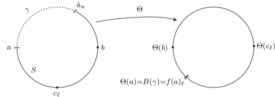
Figure 4. The circle $S$ and the map $\Theta\colon[a,{{\hat{a}}}_{u})\to S$

Definition 4.1 provides an injective function ${{\mathbf{e}}}\colon S\to{{\widehat{I}}}$ with image the set of extreme elements of ${{\widehat{I}}}$. This map is clearly discontinuous, since ${{\widehat{I}}}$ does not contain a circle: its discontinuity set is discussed in Lemma 4.5(d) and Remark 4.10.

Similarly, we define a symbolic version ${{\mathcal{E}}}\colon S\setminus\{a,b\}\to{\{0,1\}^{{\mathbb{N}}}}$ by ${{\mathcal{E}}}(x_{\ell})={{\mathcal{L}}}_{x}$ and ${{\mathcal{E}}}(x_{u})={{\mathcal{U}}}_{x}$, so that ${{\mathcal{E}}}(y)$ is an itinerary of ${{\mathbf{e}}}(y)$ for each $y\in S\setminus\{a,b\}$ (recall that ${{\mathcal{L}}}_{x}$ and ${{\mathcal{U}}}_{x}$ are the minimum and maximum itineraries in the fiber $\left[x\right]$).

If $\Theta\colon[a,{{\hat{a}}}_{u})\to S$ is defined (see Figure 4) by

$$\begin{array}[]{rcll}\Theta(x_{\ell})&=&f(x)_{\ell}&\text{ if }x\in[a,c]\\ \Theta(x_{\ell})&=&f(x)_{u}&\text{ if }x\in[c,b],\quad\text{ and}\\ \Theta(x_{u})&=&f(x)_{\ell}&\text{ if }x\in({{\hat{a}}},b],\end{array}$$ (3)

then it follows from Lemma 4.2 — and of course this is the point of the definition — that

$${{\widehat{f}}}({{\mathbf{e}}}(y))={{\mathbf{e}}}(\Theta(y))\qquad\text{for all }y\in[a,{{\hat{a}}}_{u})$$ (4)

(if $y\in[{{\hat{a}}}_{u},a)$ then ${{\widehat{f}}}({{\mathbf{e}}}(y))$ is not an extreme point by Lemma 4.2).

$\Theta$ is a continuous bijection, whose inverse has a one-sided discontinuity at $f(a)_{\ell}$ — it is discontinuous as we approach $f(a)_{\ell}$ in the positive sense — and is continuous elsewhere.

$\Theta$ can be extended to a continuous monotone circle map $B\colon S\to S$ of degree 1 by setting $B(y)=f(a)_{\ell}$ for all $y\in\gamma:=[{{\hat{a}}}_{u},a]$. $B$ is called the outside map associated to the tent map $f$ (Figure 5). We write ${\mathring{\gamma}}:=({{\hat{a}}}_{u},a)$ for the interior of $\gamma$.

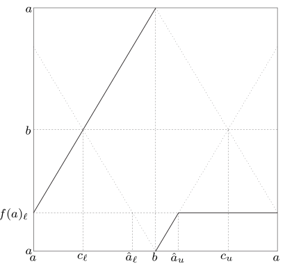
Figure 5. The outside map $B\colon S\to S$. $\Theta$ has the same graph, except that it is undefined on the interval $[{{\hat{a}}}_{u},a)$, on which $B$ takes the constant value $f(a)_{\ell}$.

The next lemma gathers some straightforward facts about $\Theta$.

Lemma 4.5.

1. If $\Theta^{r}(y)$ exists for some $r>0$, then $\tau(\Theta^{r}(y))=f^{r}(\tau(y))$.

2. $\Theta^{-r}(y)$ exists for all $y\in S$ and all $r\in{{\mathbb{N}}}$, and ${{\mathbf{e}}}(\Theta^{-r}(y))={{\widehat{f}}}^{-r}({{\mathbf{e}}}(y))$

3. An explicit formula for ${{\mathbf{e}}}(y)$ is given by

   $${{\mathbf{e}}}(y)=\left<\tau(y),\,\,\tau(\Theta^{-1}(y)),\,\,\tau(\Theta^{-2}(y)),\,\,\dots\right>.$$

4. ${{\mathbf{e}}}$ is discontinuous at $y\in S$ if and only if $y\in\operatorname{orb}(f(a)_{\ell},\Theta)$, and these discontinuities are one-sided (as we approach $y$ in the positive sense).

5. ${{\mathcal{E}}}\colon S\setminus\{a,b\}\to{\{0,1\}^{{\mathbb{N}}}}$ is locally constant at $y\in S\setminus\{a,b\}$ if and only if $y\not\in\overline{\operatorname{orb}(f(a)_{\ell},\Theta)}$.

Proof.

(a) and (b) are immediate from (3) and (4) respectively.

1. We have ${{\mathbf{e}}}(y)=\left<\pi_{0}({{\mathbf{e}}}(y)),\,\,\pi_{0}({{\widehat{f}}}^{-1}({{\mathbf{e}}}(y))),\,\,\pi_{0}({{\widehat{f}}}^{-2}({{\mathbf{e}}}(y))),\,\,\dots\right>$ by (1), and (b) gives ${{\widehat{f}}}^{-r}({{\mathbf{e}}}(y))={{\mathbf{e}}}(\Theta^{-r}(y))\in\left[\tau(\Theta^{-r}(y))\right]$, so that $\pi_{0}({{\widehat{f}}}^{-r}({{\mathbf{e}}}(y)))=\tau(\Theta^{-r}(y))$.

2. follows from (c) because $\Theta^{-1}$ has a one-sided discontinuity at $f(a)_{\ell}$ and is continuous elsewhere.

3. Since $c_{u}$ is not in the domain of $\Theta$, it follows from (c) that ${{\mathbf{e}}}(y)_{r}=c$ for some $r\geq 1$ if and only if $y\in\operatorname{orb}(\Theta(c_{\ell}),\Theta)=\operatorname{orb}(b,\Theta)=\{a,b\}\cup\operatorname{orb}(f(a)_{\ell},\Theta)$.

∎

From parts (d) and (e) of this Lemma, we see that the $\Theta$-orbit of $f(a)_{\ell}$ plays an important rôle in understanding the structure of the extreme elements of ${{\widehat{I}}}$. In particular, there is a strong distinction between the cases where this orbit is finite and those where it is infinite. Note carefully that the orbit can be finite not only when it is periodic or preperiodic, but also, more commonly, when $\Theta^{r}(f(a)_{\ell})\in[{{\hat{a}}}_{u},a)$ is outside the domain of $\Theta$ for some $r$ (see Theorem 4.8(c)).

4.3. Dynamics of the outside map

The outside map was defined in [22], and a closely related map was introduced in [18]. In this section we state those of its dynamical properties which we will use and make some related definitions. Theorem 4.7, parts (a) and (b) of Theorem 4.8, and part (a) of Theorem 4.9 can be found in [25]; while the remaining parts of Theorems 4.8 and 4.9 are proved in [14].

Definition 4.6 (Height).

The height $q_{\lambda}=q(f_{\lambda})$ of $f$ is the Poincaré rotation number of the outside map $B\colon S\to S$.

Theorem 4.7.

$q_{\lambda}$ is decreasing in $\lambda$, and $q_{\lambda}\in(0,1/2)$ for all $\lambda$. (In fact, for general tent maps, $q_{\lambda}=0$ if and only if $\lambda=2$, and $q_{\lambda}=1/2$ if and only if $\lambda\in(1,\sqrt{2}]$.)

Theorem 4.8 (The rational height case).

Let $m/n\in(0,1/2)$ be rational.

1. There is a non-trivial closed interval $\Lambda_{m/n}=[\lambda_{m/n}^{-},\lambda_{m/n}^{+}]\subset(\sqrt{2},2)$ of parameters such that $q_{\lambda}=m/n$ if and only if $\lambda\in\Lambda_{m/n}$.

2. The critical orbit of $f_{\lambda}$ is periodic (with period $n$) if $\lambda=\lambda_{m/n}^{-}$, and pre-periodic (to period $n$) if $\lambda=\lambda_{m/n}^{+}$.

3. For each $\lambda\in\Lambda_{m/n}$, the smallest positive integer $r$ with $\Theta^{r}(a)\in\gamma=[{{\hat{a}}}_{u},a]$ is $r=n$. We have $\Theta^{n}(a)=a$ if $\lambda=\lambda_{m/n}^{-}$; $\Theta^{n}(a)={{\hat{a}}}_{u}$ if $\lambda=\lambda_{m/n}^{+}$; and $\Theta^{n}(a)\in({{\hat{a}}}_{u},a)$ if $\lambda\in\operatorname{Int}(\Lambda_{m/n})$. Moreover, there is a unique $\lambda=\lambda_{m/n}^{\ast}\in\Lambda_{m/n}$ for which $\Theta^{n}(a)=c_{u}$.

4. For each $\lambda\in\Lambda_{m/n}$, the set $S\setminus\bigcup_{r\geq 0}B^{-r}({\mathring{\gamma}})$ of points whose $B$-orbits never enter ${\mathring{\gamma}}=({{\hat{a}}}_{u},a)$ is a period $n$ orbit of $B$, which attracts the $\Theta^{-1}$-orbit of every point of $S$.

Note that, by (4), we have $\Theta^{n}(a)=f^{n}(a)_{u}$ whenever $\lambda\in\Lambda_{m/n}$.

Theorem 4.9 (The irrational height case).

Let $q\in(0,1/2)$ be irrational.

1. There is a parameter $\lambda_{q}\in(\sqrt{2},2)$ such that $q_{\lambda}=q$ if and only if $\lambda=\lambda_{q}$.

2. If $\lambda=\lambda_{q}$ then $f$ is post-critically infinite. Moreover $\operatorname{orb}(f(a)_{\ell},\Theta)$ is disjoint from $\gamma=[{{\hat{a}}}_{u},a]$, and the closure of this orbit is a Cantor set ${{\mathcal{C}}}_{S}=S\setminus\bigcup_{r\geq 0}\Theta^{-r}({\mathring{\gamma}})$, the set of points whose $\Theta$-orbit never enters ${\mathring{\gamma}}$. In particular ${{\mathcal{C}}}_{S}$ contains $a$ and ${{\hat{a}}}_{u}$, since $\Theta(a)=f(a)_{\ell}$ has an orbit which never enters $\gamma$; and $\Theta$ is not defined at ${{\hat{a}}}_{u}$.

The values of $\lambda_{m/n}^{\pm}$, $\lambda_{m/n}^{\ast}$, and $\lambda_{q}$ can be specified in terms of the kneading sequences of the corresponding tent maps (see for example [14]), but this will not be necessary here.

Remark 4.10.

Using Lemma 4.5(d) and (e), it follows from Theorem 4.8(c) that if $q_{\lambda}=m/n$ then ${{\mathbf{e}}}\colon S\to{{\widehat{I}}}$ has exactly $n$ discontinuities, and ${{\mathcal{E}}}\colon S\setminus\{a,b\}\to{\{0,1\}^{{\mathbb{N}}}}$ is constant on each component of the complement of these discontinuities. (If $\lambda=\lambda_{m/n}^{-}$ then the $\Theta$-orbit of $f(a)_{\ell}$ is periodic, while if $\lambda>\lambda_{m/n}^{-}$ then it is a finite orbit segment.)

We can use Theorems 4.8 and 4.9 to classify tent maps: first, according as their height is rational or irrational; and second, in the rational case, according as the parameter $\lambda$ is an endpoint of the rational height interval, the special interior value for which $\Theta^{n}(a)=c_{u}$, or a general interior value.

Definitions 4.11 (Type of tent map: irrational, rational, endpoint, NBT, general).

We say that $f_{\lambda}$ is of irrational or rational type according as $q_{\lambda}$ is irrational or rational. In the rational case with $q_{\lambda}=m/n$, we say that $f_{\lambda}$ is of endpoint type if $\lambda=\lambda_{m/n}^{\pm}$; of NBT type if $\lambda=\lambda_{m/n}^{\ast}$; and of general type otherwise.

5. The rational post-critically infinite case

Throughout this section we assume that $f$ is of rational type with height $q=m/n$, and that the critical orbit is not periodic or pre-periodic. We will show that the corresponding sphere homeomorphism $F\colon\Sigma\to\Sigma$ is a measurable pseudo-Anosov map. (In the case where $f$ is post-critically finite, $F$ is a generalized pseudo-Anosov map, as proved in [22]: see Section 6.4.)

The path that we take is as follows:

• The map $g\colon{{\widehat{I}}}\to\Sigma$ which semi-conjugates ${{\widehat{f}}}$ to $F$ sends most of the $\pi_{0}$-fibers $\left[x\right]$ in ${{\widehat{I}}}$ — those for which $x$ is not in the grand orbit of $c$ — to arcs in $\Sigma$. In Section 5.1 we describe $g$ (recalling results from [14]) and prove this result (Theorem 5.6).

• The streamlines of the stable turbulation are unions of these arcs, joined at their endpoints. The stable measure comes from the measures $\alpha_{x}$ of Lemma 3.21 supported on the $\pi_{0}$-fibers. In Section 5.2 we define $({{\mathcal{T}}}^{s},\nu^{s})$ (Definition 5.13) and show that $F$ contracts $\nu^{s}$ by a factor $\lambda$ (Lemma 5.14) and that the turbulation is tame (Lemma 5.16).

• The streamlines of the unstable turbulation are the $g$-images of the globally leaf regular path components of ${{\widehat{I}}}$ (Definition 3.29): recall from Theorem 3.30 that the union of these has full measure — we omit countably many of them, on which the identifications induced by $g$ are non-trivial. The unstable measure comes from Lebesgue measure on the components of the $0$-flat decompositions (Lemma 3.31) of these path components. In Section 5.3 we define $({{\mathcal{T}}}^{u},\nu^{u})$ (Definition 5.17) and show that $F$ expands $\nu^{u}$ by a factor $\lambda$ (Lemma 5.18) and that the turbulation is tame (Lemma 5.19).

• In Section 5.4 we complete the proof that $F$ is a measurable pseudo-Anosov map, by proving that the two measured turbulations are transverse and full.

5.1. The semi-conjugacy $g\colon{{\widehat{I}}}\to\Sigma$

We now describe the identifications on ${{\widehat{I}}}$ realized by the semiconjugacy $g\colon{{\widehat{I}}}\to\Sigma$, and show that, under these identifications, the $\pi_{0}$-fibers of points $y\in I$ which are not on the grand orbit

$$\operatorname{GO}(c)=\{x\in I\,:\,f^{m}(x)=f^{n}(c)\text{ for some }m,n\geq 0\}$$

of $c$ become arcs in $\Sigma$.

Notation 5.1 ($\Pi$, ${{\mathbf{P}}}$).

We write $\Pi=S\setminus\bigcup_{r\geq 0}B^{-r}({\mathring{\gamma}})$, the set of points whose $B$-orbits never enter ${\mathring{\gamma}}=({{\hat{a}}}_{u},a)$, and ${{\mathbf{P}}}={{\mathbf{e}}}(\Pi)\subset{{\widehat{I}}}$.

Lemma 5.2.

$\Pi$ is a period $n$ orbit of $B$ which is disjoint from $\gamma$, and ${{\mathbf{P}}}$ is a period $n$ orbit of ${{\widehat{f}}}$ contained in the set of extreme elements of ${{\widehat{I}}}$.

Proof.

Theorem 4.8(d) states that $\Pi$ is a period $n$ orbit of $B$. By definition it is disjoint from ${\mathring{\gamma}}$, so we need only show that the endpoints $a$ and ${{\hat{a}}}_{u}$ of $\gamma$ are not in $\Pi$. Since $f$ is not post-critically finite we have $\lambda\in\operatorname{Int}(\Lambda_{m/n})$ by Theorem 4.8(b), and hence $B^{n}(a)=\Theta^{n}(a)\in{\mathring{\gamma}}$ by Theorem 4.8(c), so that $a\not\in\Pi$. Since $B(a)=B({{\hat{a}}}_{u})=f(a)_{\ell}$, we have ${{\hat{a}}}_{u}\not\in\Pi$ also.

It follows from (4) that ${{\mathbf{P}}}={{\mathbf{e}}}(\Pi)$ is a period $n$ orbit of ${{\widehat{f}}}$, which is clearly contained in the image of ${{\mathbf{e}}}$, the set of extreme elements of ${{\widehat{I}}}$. ∎

Notation 5.3 ($z$, ${{\mathcal{Z}}}$).

We write $z=f^{n}(a)$, so that $\Theta^{n}(a)=z_{u}$, and ${{\mathcal{Z}}}=\{z,{{\hat{z}}}\}$.

The following key lemma is a translation into the language of this paper of remark 5.17(e) of [14].

Lemma 5.4.

The semi-conjugacy $g\colon{{\widehat{I}}}\to\Sigma$ is the quotient map of the equivalence relation on ${{\widehat{I}}}$ with the following non-trivial equivalence classes:

1. $\{{{\widehat{f}}}^{r}\left({{\mathbf{e}}}(x_{u})\right),{{\widehat{f}}}^{r}\left({{\mathbf{e}}}({{\hat{x}}}_{u})\right)\}$, for each $x\in(a,c)\setminus{{\mathcal{Z}}}$ and each $r\in{{\mathbb{Z}}}$.

2. $\{{{\widehat{f}}}^{r}\left({{\mathbf{e}}}({{\hat{z}}}_{u})\right),{{\widehat{f}}}^{r+n}\left({{\mathbf{e}}}(a)\right),{{\widehat{f}}}^{r+n}\left({{\mathbf{e}}}({{\hat{a}}}_{u})\right)\}$, for each $r\in{{\mathbb{Z}}}$.

3. The period $n$ orbit ${{\mathbf{P}}}$.

We first use this result to understand the identifications induced by $g$ on individual fibers of ${{\widehat{I}}}$. Note that the condition $y\in I\setminus\operatorname{GO}(c)$ implies that $y\not\in{\text{PC}}$, so that the fiber $\left[y\right]$ is totally ordered, and in particular consecutive elements are well defined.

Lemma 5.5 (Identifications within fibers).

Let $y\in\operatorname{GO}(c)$.

1. Non-extreme elements of $\left[y\right]$ are only identified with other (non-extreme) elements of $\left[y\right]$.

2. Distinct non-extreme elements ${{\mathbf{x}}}$ and ${{\mathbf{x}}}^{\prime}$ of $\left[y\right]$ are identified if and only if they are consecutive.

3. The extreme elements ${{\mathbf{e}}}(y_{u})$ and ${{\mathbf{e}}}(y_{\ell})$ of $\left[y\right]$ are not identified with each other: that is, $g({{\mathbf{e}}}(y_{u}))\not=g({{\mathbf{e}}}(y_{\ell}))$.

Proof.

1. Since $y\not\in\operatorname{GO}(c)$, equivalence classes of type (EII) are disjoint from $\left[y\right]$. Moreover, if $r\geq 0$ then for any $x\in(a,c)\setminus{{\mathcal{Z}}}$ we have ${{\widehat{f}}}^{-r}({{\mathbf{e}}}(x_{u}))={{\mathbf{e}}}(\Theta^{-r}(x_{u}))$ and ${{\widehat{f}}}^{-r}({{\mathbf{e}}}({{\hat{x}}}_{u}))={{\mathbf{e}}}(\Theta^{-r}({{\hat{x}}}_{u}))$ by Lemma 4.5(b), so these are extreme elements, as are the points of ${{\mathbf{P}}}$. Therefore the non-trivial equivalence classes which contain non-extreme elements of $\left[y\right]$ are precisely $\{{{\widehat{f}}}^{r}\left({{\mathbf{e}}}(x_{u})\right),{{\widehat{f}}}^{r}\left({{\mathbf{e}}}({{\hat{x}}}_{u})\right)\}$ for those $x\in(a,c)\setminus{{\mathcal{Z}}}$ and $r>0$ which satisfy $f^{r}(x)=y$; and, since $f^{r}(x)=f^{r}({{\hat{x}}})$, such equivalence classes consist of two points of $\left[y\right]$.

2. Suppose that ${{\mathbf{x}}}$ and ${{\mathbf{x}}}^{\prime}$ are consecutive. Let $r>0$ be least such that $x_{r}\not=x_{r}^{\prime}$. By Lemma 4.3(b) and (c), we have ${{\widehat{f}}}^{-r}({{\mathbf{x}}})={{\mathbf{e}}}(x_{r,u})$ and ${{\widehat{f}}}^{-r}({{\mathbf{x}}}^{\prime})={{\mathbf{e}}}(x^{\prime}_{r,u})$. Since $x^{\prime}_{r}=\widehat{x_{r}}$ (both have image $x_{r-1}$), and these are not equal to $a$, $c$, $z$, or ${{\hat{z}}}$ (since $y\not\in\operatorname{GO}(c)$), it follows from (EI) that $g({{\mathbf{x}}})=g({{\mathbf{x}}}^{\prime})$ as required.

   For the converse, if $g({{\mathbf{x}}})=g({{\mathbf{x}}}^{\prime})$ then by the proof of (a) there are $x\in(a,c)\setminus{{\mathcal{Z}}}$ and $r>0$ such that $\{{{\mathbf{x}}},{{\mathbf{x}}}^{\prime}\}=\{{{\widehat{f}}}^{r}({{\mathbf{e}}}(x_{u})),{{\widehat{f}}}^{r}({{\mathbf{e}}}({{\hat{x}}}_{u}))\}$. These are consecutive by Lemma 4.3(d) and (a).

3. The two extreme elements cannot both belong to the periodic orbit ${{\mathbf{P}}}$, since if $y<{{\hat{a}}}$ then $y_{u}\in{\mathring{\gamma}}$ (so that $y_{u}\not\in\Pi$, and hence ${{\mathbf{e}}}(y_{u})\not\in{{\mathbf{P}}}$); while if $y>{{\hat{a}}}$ then $f(y)<f(a)<{{\hat{a}}}$ by Lemma 3.8, and hence $B(y_{\ell})=f(y)_{u}\in{\mathring{\gamma}}$ (so that $y_{\ell}\not\in\Pi$, and hence ${{\mathbf{e}}}(y_{\ell})\not\in{{\mathbf{P}}}$).

   It follows from Lemma 5.4 and $y\not\in\operatorname{GO}(c)$ that we could only have $g({{\mathbf{e}}}(y_{u}))=g({{\mathbf{e}}}(y_{\ell}))$ if there were some $x\in(a,c)$ and $r\in{{\mathbb{Z}}}$ with $\{{{\mathbf{e}}}(y_{u}),{{\mathbf{e}}}(y_{\ell})\}$ equal to $\{{{\widehat{f}}}^{r}\left({{\mathbf{e}}}(x_{u})\right),{{\widehat{f}}}^{r}\left({{\mathbf{e}}}({{\hat{x}}}_{u})\right)\}$. However if $r>0$ then ${{\widehat{f}}}^{r}\left({{\mathbf{e}}}(x_{u})\right)$ and ${{\widehat{f}}}^{r}\left({{\mathbf{e}}}({{\hat{x}}}_{u})\right)$ are non-extreme elements of $\left[f^{r}(x)\right]$. If $r=-s\leq 0$, on the other hand, then we would have $\{y_{u},y_{\ell}\}=\{\Theta^{-s}(x_{u}),\Theta^{-s}({{\hat{x}}}_{u})\}$ as in the proof of (a), so that $s$ would be both least with $B^{s}(y_{u})\in{\mathring{\gamma}}$, and least with $B^{s}(y_{\ell})\in{\mathring{\gamma}}$. This is impossible, since, as above, if $y<{{\hat{a}}}$ then $y_{u}\in{\mathring{\gamma}}$ but $y_{\ell}\not\in{\mathring{\gamma}}$; while if $y>{{\hat{a}}}$ then $B(y_{\ell})\in{\mathring{\gamma}}$ but $B(y_{u})=f(y)_{\ell}\not\in{\mathring{\gamma}}$.

∎

Theorem 5.6.

Let $y\in I\setminus\operatorname{GO}(c)$. Then $g(\left[y\right])$ is an arc in $\Sigma$.

Proof.

Let $H\colon{\{0,1\}^{{\mathbb{N}}}}\to[0,1]$ be the order-preserving homeomorphism onto the middle thirds Cantor set defined by

$$H(s)=\sum_{r=0}^{\infty}\frac{2\varepsilon_{r}}{3^{r}},\quad\text{ where }\varepsilon_{r}=\left(\sum_{i=0}^{r}s_{i}\right)\bmod{2}.$$

Then $H\circ J\colon\left[y\right]\to[0,1]$ is an order-preserving embedding of the Cantor set $\left[y\right]$ into the interval. Therefore, by Lemma 5.5(b) and (c), $g(\left[y\right])$ is homeomorphic to the space obtained by collapsing the complementary intervals of a Cantor subset of the interval: that is, to an arc. ∎

Notation 5.7 (${{\mathcal{A}}}_{y}$).

For each $y\in I\setminus\operatorname{GO}(c)$, we write ${{\mathcal{A}}}_{y}$ for the arc $g(\left[y\right])\subset\Sigma$.

Lemma 5.8.

For $y\in I\setminus\operatorname{GO}(c)$, let ${{\mathcal{B}}}_{y}$ be the subset of ${{\mathcal{A}}}_{y}$ consisting of points with a unique $g$-preimage. Then $g^{-1}\colon{{\mathcal{B}}}_{y}\to\left[y\right]$ is continuous.

Proof.

Suppose for a contradiction that there is a convergent sequence $x_{n}\to x$ in ${{\mathcal{B}}}_{y}$ with $g^{-1}(x_{n})\not\to g^{-1}(x)$. Since $\left[y\right]$ is compact, we can assume by taking a subsequence that $g^{-1}(x_{n})\to{{\mathbf{x}}}\not=g^{-1}(x)$. Since $g$ is continuous, it follows that $x_{n}\to g({{\mathbf{x}}})$, so that $x=g({{\mathbf{x}}})$. The distinct elements ${{\mathbf{x}}}$ and $g^{-1}(x)$ of $\left[y\right]$ are therefore both mapped to $x$ by $g$, contradicting the assumption that $x\in{{\mathcal{B}}}_{y}$. ∎

5.2. The stable turbulation

The streamlines of the stable turbulation will be formed from unions of the arcs ${{\mathcal{A}}}_{y}$, which are joined at their endpoints by the identifications of Lemma 5.4. In order to ensure that the endpoints are identified in pairs, we need to exclude the identifications of types (EII) and (EIII) in Lemma 5.4. Type (EII) identifications are excluded in any case, since $y\not\in\operatorname{GO}(c)$; to deal with type (EIII), we will also require that $y$ is not in the grand orbit of $\pi_{0}({{\mathbf{P}}})$.

Notation 5.9 ($P$, $V$, $\mu$).

Write $P=\pi_{0}({{\mathbf{P}}})$ and let $V=I\setminus(\operatorname{GO}(c)\cup\operatorname{GO}(P))$, a totally $f$-invariant subset of $I$ with countable complement.

Denote by $\mu$ the OU ergodic $F$-invariant probability measure $g_{*}({{\hat{\mu}}})$ on $\Sigma$, where ${{\hat{\mu}}}$ is the measure on ${{\widehat{I}}}$ defined in Section 3.3. No confusion will arise from the same symbol’s having been used for the absolutely continuous $f$-invariant measure on $I$.

If $y\in V$ then, by definition of ${{\mathbf{P}}}$, there is some $r\geq 0$ with $B^{r}(y_{u})\in({{\hat{a}}}_{u},a)$: say $B^{r}(y_{u})=x_{u}$. Then $x\not\in{{\mathcal{Z}}}$, since $y\not\in\operatorname{GO}(c)$, and hence, by Lemma 5.4, ${{\mathbf{e}}}(y_{u})={{\mathbf{e}}}(B^{-r}(x_{u}))$ is identified with ${{\mathbf{e}}}(B^{-r}({{\hat{x}}}_{u}))$, and only with this point.

That is, for every $y\in V$ there is a unique $x\in V\setminus\{y\}$ such that $g({{\mathbf{e}}}(y_{u}))$ is an endpoint of ${{\mathcal{A}}}_{x}$; and, by an identical argument, there is a unique $x^{\prime}\in V\setminus\{y\}$ such that $g({{\mathbf{e}}}(y_{\ell}))$ is an endpoint of ${{\mathcal{A}}}_{x^{\prime}}$.

It follows that for every $y\in V$, there is a bi-infinite sequence $(y_{i})_{i\in{{\mathbb{Z}}}}$ in $V$ with $y_{0}=y$ and $y_{i}\not=y_{i+1}$ for each $i$, unique up to reversal, such that each ${{\mathcal{A}}}_{y_{i}}$ shares one endpoint with ${{\mathcal{A}}}_{y_{i-1}}$ and the other with ${{\mathcal{A}}}_{y_{i+1}}$.

Notation 5.10 ($\ell_{y}$).

For each $y\in V$ we write $\ell_{y}=\bigcup_{i\in{{\mathbb{Z}}}}{{\mathcal{A}}}_{y_{i}}$, which is either an immersed line, or, if the sequence $(y_{i})$ repeats, a simple closed curve. We shall see in Lemma 5.15 that the latter is impossible.

The $\ell_{y}$ will be the streamlines of the stable turbulation, and we now define the stream measures.

Definition 5.11 ($\nu^{s}_{\ell_{y}}$).

We define a Borel measure $\nu^{s}_{\ell_{y}}$ on $\ell_{y}$ by

$$\nu^{s}_{\ell_{y}}=\sum_{i\in K}g_{*}(\alpha_{y_{i}}),$$

where the $\alpha_{y_{i}}$ are the measures of Lemma 3.21, supported on $\left[y_{i}\right]$; and where $K={{\mathbb{Z}}}$ if the $y_{i}$ are all distinct, and otherwise $K=\{0,\dots,r-1\}$ if $r>0$ is least with $y_{r}=y_{0}$. Notice from Lemma 3.21 that $\nu^{s}_{\ell_{y}}({{\mathcal{A}}}_{y_{i}})=\varphi(y_{i})$.

The next lemma ensures that the streamlines and stream measures satisfy the conditions of Definitions 2.11.

Lemma 5.12.

1. $\mu\left(\bigcup_{y\in V}\ell_{y}\right)=1$.

2. The measures $\nu^{s}_{\ell_{y}}$ are OU and assign finite measure to closed arcs.

Proof.

Write $X=\bigcup_{y\in V}\ell_{y}$, and note that $X=g(\pi_{0}^{-1}(V))$. Since $V$ has countable complement, Theorem 3.28 gives

$$\mu(X^{s})={{\hat{\mu}}}(\pi_{0}^{-1}(V))=\int_{V}\alpha_{x}(\left[x\right])dm(x)=\int_{I}\alpha_{x}(\left[x\right])dm(x)={{\hat{\mu}}}({{\widehat{I}}})=\mu(\Sigma).$$

$\nu^{s}_{\ell_{y}}$ is OU since the same is true of each $\alpha_{y_{i}}$ (Remarks 3.22(a)). Every closed arc in $\ell_{y}$ is contained in a finite union of the ${{\mathcal{A}}}_{y_{i}}$, and so has finite measure. ∎

Until we show in Lemma 5.15 that all of the $\ell_{y}$ are immersed lines, we temporarily relax the definition of measured turbulation to allow streamlines which are simple closed curves.

Definition 5.13 (${{\mathcal{T}}}^{s},\nu^{s}$).

We define the stable turbulation $({{\mathcal{T}}}^{s},\nu^{s})$ on $\Sigma$ to be the measured turbulation whose streamlines are the distinct immersed lines and simple closed curves $\ell_{y}$, for $y\in V$, with measure $\nu^{s}_{\ell_{y}}$ on the streamline $\ell_{y}$.

Lemma 5.14.

$F({{\mathcal{T}}}^{s},\nu^{s})=({{\mathcal{T}}}^{s},\lambda\nu^{s})$.

Proof.

$F$ sends streamlines to streamlines since ${{\widehat{f}}}$ sends $\pi_{0}$-fibers into $\pi_{0}$-fibers and respects the identifications of Lemma 5.4.

If $A$ is a Borel subset of a streamline $\ell_{y}$ then $\nu^{s}_{\ell_{y}}(A)=\sum_{i\in K}\alpha_{y_{i}}(g^{-1}(A))$, where $K={{\mathbb{Z}}}$ or $K=\{0,\dots,r-1\}$ as in Definition 5.11. On the other hand

$$\nu^{s}_{\ell_{f(y)}}(F(A)) = \sum_{i\in K}\alpha_{f(y_{i})}(g^{-1}(F(A)))$$

$$= \sum_{i\in K}\alpha_{f(y_{i})}({{\widehat{f}}}(g^{-1}(A)))$$

$$= \lambda^{-1}\sum_{i\in K}\alpha_{y_{i}}(g^{-1}(A))=\lambda^{-1}\nu^{s}_{\ell_{y}}(A),$$

where the first equality comes from $F({{\mathcal{A}}}_{y_{i}})\subset{{\mathcal{A}}}_{f(y_{i})}$; the second is because $g$ is almost everywhere invertible; and the third comes from Remarks 3.22(b).

Thus $F_{*}(\nu^{s}_{\ell_{y}})=\lambda\nu^{s}_{\ell_{f(y)}}$ as required. ∎

Lemma 5.15.

Every streamline of $({{\mathcal{T}}}^{s},\nu^{s})$ is dense in $\Sigma$. In particular, no streamlines are simple closed curves, so that $({{\mathcal{T}}}^{s},\nu^{s})$ is a measured turbulation.

Proof.

Let $U\subset\Sigma$ be non-empty and open, and $\ell_{y}$ be a streamline: we shall show that they intersect.

$g^{-1}(U)$ is open in ${{\widehat{I}}}$, so $\pi_{0}(g^{-1}(U))$ contains an interval $J\subset I$ (one way to see this is from Theorem 3.30 and Lemma 3.31: $g^{-1}(U)$ contains an open arc in ${{\widehat{I}}}$, which has a $0$-flat decomposition). Tent maps with slope $\lambda>\sqrt{2}$ are locally eventually onto, so that there is some $n>0$ with $f^{n}(J)=I$. In particular, there is some $x\in J$ with $f^{n}(x)=f^{n}(y)$: thus ${{\widehat{f}}}^{n}(\left[x\right])\subset\left[f^{n}(y)\right]$ and ${{\widehat{f}}}^{n}(\left[y\right])\subset\left[f^{n}(y)\right]$, so that both $\left[x\right]$ and $\left[y\right]$ are contained in ${{\widehat{f}}}^{-n}(\left[f^{n}(y)\right])$. Applying $g$, both ${{\mathcal{A}}}_{x}$ and ${{\mathcal{A}}}_{y}$ are contained in $F^{-n}({{\mathcal{A}}}_{f^{n}(y)})$. Since $F^{-n}({{\mathcal{A}}}_{f^{n}(y)})$ is a stream arc containing ${{\mathcal{A}}}_{y}$, the streamline which contains it is $\ell_{y}$. Thus ${{\mathcal{A}}}_{x}\subset\ell_{y}$: but since $x\in J\subset\pi_{0}(g^{-1}(U))$ we have ${{\mathcal{A}}}_{x}\cap U\not=\emptyset$. ∎

Therefore $({{\mathcal{T}}}^{s},\nu^{s})$ is a measured turbulation with dense streamlines, which satisfies $F({{\mathcal{T}}}^{s},\nu^{s})=({{\mathcal{T}}}^{s},\lambda\nu^{s})$. It remains to show that it is tame (Definition 2.13).

Lemma 5.16.

$({{\mathcal{T}}}^{s},\nu^{s})$ is tame.

Proof.

Let $\rho$ be a metric on $\Sigma$ inducing its topology, and let $\epsilon>0$. Let $\xi>0$ be small enough that $d({{\mathbf{x}}},{{\mathbf{y}}})<\xi\implies\rho(g({{\mathbf{x}}}),g({{\mathbf{y}}}))<\epsilon/2$, where $d$ is the standard metric of Definitions 3.9.

Let $k>0$ be a lower bound for the density $\varphi$ of Section 3.3 on $V\subset I\setminus{\text{PC}}$. Let $r>0$ be an integer large enough that $1/2^{r}<\xi$, and set $\delta=k/\lambda^{r}$. We shall show that any stream arc $[u,v]$ with measure less than $\delta$ satisfies $\rho(u,v)<\epsilon$, establishing tameness of the turbulation.

Recall from Definitions 3.11 that, given our fixed integer $r>0$, each fiber $\left[x\right]$ of ${{\widehat{I}}}$ is partitioned into a finite number of level $r$ cylinder sets

$$\left[x,y_{1},\dots,y_{r}\right]=\{{{\mathbf{x}}}\in\left[x\right]\,:\,x_{i}=y_{i}\text{ for }1\leq i\leq r\},$$

where $f(y_{1})=x$ and $f(y_{i})=y_{i-1}$ for $2\leq i\leq r$. If $x\in V$, so that $x\not\in{\text{PC}}$ and itineraries are well-defined on $\left[x\right],$ then each of these cylinder sets corresponds to a choice of the first $r$ symbols of the itinerary of ${{\mathbf{x}}}$: in particular, given two distinct level $r$ cylinder subsets $C_{1}$ and $C_{2}$ of $\left[x\right]$, either $J({{\mathbf{x}}})\prec J({{\mathbf{x}}}^{\prime})$ for every ${{\mathbf{x}}}\in C_{1}$ and ${{\mathbf{x}}}^{\prime}\in C_{2}$, or $J({{\mathbf{x}}}^{\prime})\prec J({{\mathbf{x}}})$ for every ${{\mathbf{x}}}\in C_{1}$ and ${{\mathbf{x}}}^{\prime}\in C_{2}$. It follows that the image $g(\left[x,y_{1},\dots,y_{r}\right])$ of a cylinder set is a stream arc, which we denote ${{\mathcal{A}}}_{x,y_{1},\dots,y_{r}}$ and call a level $r$ cylinder arc. The stream arc ${{\mathcal{A}}}_{x}$ is a union of these level $r$ cylinder arcs, which intersect only at their endpoints.

By Lemma 3.21 the arc ${{\mathcal{A}}}_{x,y_{1},\dots,y_{r}}$ has measure $\varphi(y_{r})/\lambda^{r}\geq k/\lambda^{r}=\delta$, so that any stream arc of measure less than $\delta$ is contained in the union of at most two level $r$ cylinder arcs (possibly in different fibers of ${{\widehat{I}}}$). Now the metric diameter of a level $r$ cylinder set is bounded above by $\sum_{i=r+1}^{\infty}|b-a|/2^{i}<1/2^{r}<\xi$, so that the metric diameter of a level $r$ cylinder arc is bounded above by $\epsilon/2$. Therefore the endpoints $[u,v]$ of a stream arc contained in the union of at most two level $r$ cylinder arcs satisfy $\rho(u,v)<\epsilon$ as required.

∎

5.3. The unstable turbulation

The streamlines of the unstable turbulation will be $g$-images of the globally leaf regular path components (Definition 3.29) of ${{\widehat{I}}}$. We will omit the countably many path components which are involved in identifications — that is, which contain points ${{\mathbf{x}}}$ for which $g^{-1}(\{g({{\mathbf{x}}})\})\not=\{{{\mathbf{x}}}\}$.

Consider the identifications of type (EI) from Lemma 5.4. By Lemma 4.5(d), ${{\mathbf{e}}}\colon S\to{{\widehat{I}}}$ is discontinuous at $y\in S$ if and only if $y\in\operatorname{orb}(f(a)_{\ell},\Theta)$. Since there is exactly one point of this orbit in $({{\hat{a}}}_{u},a)$, namely $\Theta^{n}(a)=z_{u}$, the set of points $\{{{\mathbf{e}}}(x_{u})\,:\,x\in(a,{{\hat{a}}})\}$ is contained in at most two path components of ${{\widehat{I}}}$. The union $\Gamma_{1}$ of the bi-infinite ${{\widehat{f}}}$-orbits of these path components is therefore an ${{\widehat{f}}}$-invariant set which contains all of the points of ${{\widehat{I}}}$ involved in identifications of type (EI).

Likewise, the union $\Gamma_{2}$ of the bi-infinite ${{\widehat{f}}}$-orbits of the path components of ${{\mathbf{e}}}({{\hat{z}}}_{u})$, ${{\mathbf{e}}}(a)$, and ${{\mathbf{e}}}({{\hat{a}}}_{u})$ is an ${{\widehat{f}}}$-invariant set which contains all points involved in identifications of type (EII); and the union $\Gamma_{3}$ of the path components of the points of ${{\mathbf{P}}}$ is ${{\widehat{f}}}$-invariant and contains all points involved in identifications of type (EIII).

Let

$$K^{u}=\{{{\mathbf{x}}}\in{{\widehat{I}}}\,:\,{{\mathbf{x}}}\text{ is globally leaf regular}\}\setminus(\Gamma_{1}\cup\Gamma_{2}\cup\Gamma_{3}).$$ (5)

Then $K^{u}$ is an ${{\widehat{f}}}$-invariant union of globally leaf regular path components of ${{\widehat{I}}}$ with $g^{-1}(\{g({{\mathbf{x}}})\})=\{{{\mathbf{x}}}\}$ for all ${{\mathbf{x}}}\in K^{u}$.

Since $\Gamma_{1}\cup\Gamma_{2}\cup\Gamma_{3}$ contains only countably many of the path components of ${{\widehat{I}}}$, each of which has ${{\hat{\mu}}}$-measure zero by Remark 3.32, it follows from Theorem 3.30 that ${{\hat{\mu}}}(K^{u})={{\hat{\mu}}}({{\widehat{I}}})$.

Let $\Gamma$ be a path component of $K^{u}$. Since $\Gamma$ is an immersed line and $g$ is injective on $K^{u}$, its image $\ell=g(\Gamma)$ is also an immersed line. Moreover, $\ell$ is dense in $\Sigma$, since $\Gamma$ is dense in ${{\widehat{I}}}$ and $g$ is continuous and surjective. These dense lines $\ell$ will be the streamlines of the unstable turbulation.

We define an OU measure $\nu^{u}_{\ell}$ on $\ell$ using the $0$-flat decomposition $\Gamma=\bigcup_{i\in{{\mathbb{Z}}}}\Gamma_{i}$ of Lemma 3.31: if $A$ is a Borel subset of $\ell$, then

$$\nu^{u}_{\ell}(A)=\sum_{i\in{{\mathbb{Z}}}}m(\pi_{0}(g^{-1}(A)\cap\Gamma_{i})),$$ (6)

where $m$ is Lebesgue measure on $I$.

Every closed stream arc in $\ell$ is contained in a finite union of the arcs $g(\Gamma_{i})$ coming from the $0$-flat decomposition of $\Gamma$, and so has finite measure by (6).

Definition 5.17 (${{\mathcal{T}}}^{u},\nu^{u}$).

We define the unstable turbulation $({{\mathcal{T}}}^{u},\nu^{u})$ to be the measured turbulation on $\Sigma$ whose streamlines are the $g$-images of the path components of $K^{u}$, with measure $\nu^{u}_{\ell}$ on the streamline $\ell$.

Lemma 5.18.

$F({{\mathcal{T}}}^{u},\nu^{u})=({{\mathcal{T}}}^{u},\lambda^{-1}\nu^{u})$.

Proof.

Let $\ell=g(\Gamma)$ be a streamline of ${{\mathcal{T}}}^{u}$. Then $F(\ell)=g({{\widehat{f}}}(\Gamma))$ is also a streamline.

Let $A$ be a Borel subset of $\ell$. Write $\Gamma=\bigcup_{i\in{{\mathbb{Z}}}}\Gamma_{i}$ for the $0$-flat decomposition of Lemma 3.31, and for each $i\in{{\mathbb{Z}}}$ define measurable subsets of $A$ by

$$A_{i}^{L} = \{x\in A\,:\,g^{-1}(x)\in\Gamma_{i}\text{ and }\pi_{0}(g^{-1}(x))<c\}\text{ and}$$

$$A_{i}^{R} = \{x\in A\,:\,g^{-1}(x)\in\Gamma_{i}\text{ and }\pi_{0}(g^{-1}(x))>c\}.$$

It is enough to show that $\nu^{u}_{F(\ell)}(F(A_{i}^{Q}))=\lambda\nu^{u}_{\ell}(A_{i}^{Q})$ for each $i$ and each $Q\in\{L,R\}$.

Now $\nu^{u}_{\ell}(A_{i}^{Q})=m(\pi_{0}(g^{-1}(A_{i}^{Q})))$. Since $g^{-1}(A_{i}^{Q})$ is contained in a $0$-flat arc disjoint from $\left[c\right]$, its image ${{\widehat{f}}}(g^{-1}(A_{i}^{Q}))=g^{-1}(F(A_{i}^{Q}))$ is contained in a $0$-flat arc. Therefore, if $\bigcup_{i\in{{\mathbb{Z}}}}\delta_{i}$ is the $0$-flat decomposition of $g^{-1}(F(\ell))$, there is some $j$ for which $g^{-1}(F(A_{i}^{Q}))\subset~{}\delta_{j}$. It follows that

$$\nu^{u}_{F(\ell)}\big{(}F\big{(}A_{i}^{Q}\big{)}\big{)} = m\big{(}\pi_{0}\big{(}g^{-1}\big{(}F\big{(}A_{i}^{Q}\big{)}\big{)}\big{)}\big{)}$$

$$= m\big{(}\pi_{0}\big{(}{{\widehat{f}}}\big{(}g^{-1}\big{(}A_{i}^{Q}\big{)}\big{)}\big{)}\big{)}$$

$$= m\big{(}f\big{(}\pi_{0}\big{(}g^{-1}\big{(}A_{i}^{Q}\big{)}\big{)}\big{)}\big{)}$$

$$= \lambda m\big{(}\pi_{0}\big{(}g^{-1}\big{(}A_{i}^{Q}\big{)}\big{)}\big{)}$$

$$= \lambda\nu^{u}_{\ell}\big{(}A_{i}^{Q}\big{)}\quad\text{ as required.}$$

Here the fourth equality follows from the fact that $\pi_{0}(g^{-1}(A_{i}^{Q}))$ is contained in $[a,c]$ or in $[c,b]$, according as $Q=L$ or $Q=R$, on which $f$ expands uniformly by a factor $\lambda$. ∎

Therefore $({{\mathcal{T}}}^{u},\nu^{u})$ is a measured turbulation with dense streamlines, which satisfies $F({{\mathcal{T}}}^{u},\nu^{u})=({{\mathcal{T}}}^{u},\lambda^{-1}\nu^{u})$. It remains to show that it is tame (Definition 2.13).

Lemma 5.19.

$({{\mathcal{T}}}^{u},\nu^{u})$ is tame.

Proof.

If $\Gamma$ is a $0$-flat arc in ${{\widehat{I}}}$ over the interval $J$, then $m(\pi_{0}(\Gamma))=|J|$, while the metric diameter of $\Gamma$ is $\frac{2\lambda}{2\lambda-1}|J|<2|J|$ (see for example section 4.1 of [13]).

Let $\rho$ be a metric on $\Sigma$ inducing its topology and let $\epsilon>0$. Pick $\xi>0$ small enough that $d({{\mathbf{x}}},{{\mathbf{y}}})<\xi\implies\rho(g({{\mathbf{x}}}),g({{\mathbf{y}}}))<\epsilon$.

Let $\delta=\xi/2$, and consider a stream arc $[x,y]\subset\ell$ with $\nu_{\ell}^{u}([x,y])<\delta$. Then $g^{-1}([x,y])$ is a union of finitely many $0$-flat arcs which intersect only at their endpoints, arising from the $0$-flat decomposition of $g^{-1}(\ell)$. By (6) and the remarks above, the metric diameter of $g^{-1}([x,y])$ is less than $2\delta=\xi$, so that $\rho(x,y)<\epsilon$ as required.

∎

5.4. $F$ is a measurable pseudo-Anosov map

We have defined tame measured turbulations $({{\mathcal{T}}}^{s},\nu^{s})$ and $({{\mathcal{T}}}^{u},\nu^{u})$ on $\Sigma$, having dense streamlines, with the properties that $F({{\mathcal{T}}}^{s},\nu^{s})=({{\mathcal{T}}}^{s},\lambda\nu^{s})$ and $F({{\mathcal{T}}}^{u},\nu^{u})=({{\mathcal{T}}}^{u},\lambda^{-1}\nu^{u})$. In this section we show that these turbulations satisfy the remaining conditions of Definition 2.22, thereby establishing that $F\colon\Sigma\to\Sigma$ is measurable pseudo-Anosov. That is:

• the two turbulations are transverse (Lemma 5.20); and

• the turbulations are full: there is a countable collection of compatible tartans whose intersections cover a full measure subset of $\Sigma$, and every non-empty open subset of $\Sigma$ contains a positive measure compatible tartan (Lemma 5.21).

Lemma 5.20.

Every intersection of ${{\mathcal{T}}}^{s}$ and ${{\mathcal{T}}}^{u}$ is topologically transverse.

Proof.

Let $g({{\mathbf{x}}})$ be a point of intersection of a streamline $\ell=g(\Gamma)$ of ${{\mathcal{T}}}^{u}$, and a streamline $\ell^{\prime}$ of ${{\mathcal{T}}}^{s}$. The streamline $\ell^{\prime}$ is locally contained in the arc ${{\mathcal{A}}}_{x_{0}}$ for some $x_{0}\in V$ ($g({{\mathbf{x}}})$ cannot be an endpoint of ${{\mathcal{A}}}_{x_{0}}$, since points of $\ell$ have a unique $g$-preimage). The arc ${{\mathcal{A}}}_{x_{0}}$ separates any sufficiently small disk neighborhood of $g({{\mathbf{x}}})$ into points $g({{\mathbf{y}}})$ with $y_{0}<x_{0}$, and points $g({{\mathbf{y}}})$ with $y_{0}>x_{0}$. It is therefore enough to show that $\pi_{0}|_{\Gamma}$ is locally injective at ${{\mathbf{x}}}$. This is a consequence of Lemma 3.31: since $x_{0}\not\in\operatorname{GO}(c)$, we have $x_{r}\not=c$ for all $r$, and hence ${{\mathbf{x}}}$ is in the interior of one of the components $\Gamma_{i}$ of the $0$-flat decomposition of $\Gamma$ by Remark 3.24. ∎

Lemma 5.21.

The pair $({{\mathcal{T}}}^{s},\nu^{s})$, $({{\mathcal{T}}}^{u},\nu^{u})$ is full.

Proof.

We will prove the existence of a positive measure regular compatible tartan $R$. It follows from Lemma 2.23 and Remark 2.21 that $F^{i}(R)$ is a regular compatible tartan for each $i\geq 0$. Since $F$ is ergodic this countable collection of tartans has $\mu(\bigcup_{i\geq 0}F^{i}(R)^{\pitchfork})=1$, and fullness follows from Lemma 2.20.

By Theorem 3.26 there is a $0$-box $B$ with ${{\hat{\mu}}}(B)>0$: recall that $B$ is a disjoint union of $0$-flat arcs over some interval $J\subseteq I$. Without loss of generality we can assume that the arcs of $B$ are all contained in the full measure subset $K^{u}$ of (5), so that their images under $g$ are contained in streamlines of ${{\mathcal{T}}}^{u}$, and $g$ is injective on $B$.

Recall (Notation 5.9) that $V=I\setminus(\operatorname{GO}(c)\cup\operatorname{GO}(P))$, and write $J^{\prime}=J\cap V$, which has countable complement in $J$. Let $R^{u}=g(B)$, a disjoint union of unstable stream arcs, each with finite stream measure $m(J)$; and let $R^{s}=\bigcup_{y\in J^{\prime}}{{\mathcal{A}}}_{y}$ (recall Notation 5.7), a disjoint union of stable stream arcs with bounded stream measures $\nu_{\ell_{y}}^{s}({{\mathcal{A}}}_{y})=\varphi(y)$.

By definition, $\pi_{0}$ is a bijection from each arc of $B$ onto $J$, so that each of these arcs intersects each fiber $\left[y\right]$ (with $y\in J$) exactly once. Since $g^{-1}(x)$ is a point for each $x\in R^{u}$, it follows that every arc of $R^{s}$ intersects every arc of $R^{u}$ exactly once, and these intersections are either transverse or at endpoints by Lemma 5.20. Each unstable fiber ${{\mathfrak{u}}}$ can be oriented in the direction of increasing $\pi_{0}\circ g^{-1}\colon{{\mathfrak{u}}}\to J$, and with this orientation crosses the stable fibers ${{\mathcal{A}}}_{y}$ in order of increasing $y$. Likewise, each stable fiber can be oriented in the direction of increasing itinerary, and with this orientation crosses the unstable fibers in order of increasing itinerary (see Remark 3.24).

The open topological disk $\Sigma\setminus\{g({{\mathbf{e}}}(c^{u}))\}$ contains $R^{s}\cup R^{u}$, so $R=(R^{s},R^{u})$ is a tartan (Definition 2.15). It has positive measure by Theorem 3.28:

$$\mu(R^{\pitchfork})={{\hat{\mu}}}(B\cap\pi_{0}^{-1}(J^{\prime}))=\int_{J^{\prime}}\alpha_{x}(B)\,dm(x)=\int_{J}\alpha_{x}(B)\,dm(x)={{\hat{\mu}}}(B)>0.$$

It thus remains to show that $R$ is compatible and regular.

Given $y,z\in J^{\prime}$, there is a holonomy map $h_{y,z}\colon\left[y\right]\cap B\to\left[z\right]\cap B$, which takes the point of $\left[y\right]\cap\Gamma$ to the point of $\left[z\right]\cap\Gamma$ for each $0$-flat arc $\Gamma$ of $B$. That is, since each $0$-flat arc has constant itinerary (Remark 3.24), $h_{y,z}({{\mathbf{x}}})=L(z,J({{\mathbf{x}}}))$, where $L\colon{{\mathcal{V}}}\to{{\widehat{I}}}$ is the continuous function of Lemma 3.19. In particular, $h_{y,z}$ is a homeomorphism (with inverse $h_{z,y}$). Moreover, if $X\subseteq\left[y\right]\cap B$ is Borel, then

$$\alpha_{y}(X)=\alpha_{z}(h_{y,z}(X)),$$ (7)

by applying Theorem 3.27 to the $0$-box consisting of those $0$-flat arcs of $B$ which pass through $X$.

Now pick arbitrary stable and unstable fibers ${{\mathfrak{s}}}={{\mathcal{A}}}_{y}=g(\left[y\right])$ and ${{\mathfrak{u}}}=g(\Gamma)$ of $R$, where $y\in J^{\prime}$ and $\Gamma$ is one of the $0$-flat arcs of $B$. Define

$$\psi\colon(\left[y\right]\cap B)\times(\Gamma\cap\pi_{0}^{-1}(J^{\prime}))\to B\cap\pi_{0}^{-1}(J)$$

by $\psi({{\mathbf{x}}},{{\mathbf{x}}}^{\prime})=h_{y,\pi_{0}({{\mathbf{x}}}^{\prime})}({{\mathbf{x}}})=L(\pi_{0}({{\mathbf{x}}}^{\prime}),J({{\mathbf{x}}}))$, which is continuous by Lemma 3.19 and Remark 3.20, and so a homeomorphism with inverse $\psi^{-1}({{\mathbf{x}}})=(L(y,J({{\mathbf{x}}})),L(\pi_{0}({{\mathbf{x}}}),s))$, where $s$ is the constant itinerary of $\Gamma$. The definition is made in order that

$$\begin{CD}(\left[y\right]\cap B)\times(\Gamma\cap\pi_{0}^{-1}(J^{\prime}))@>{\psi}>{}>B\cap\pi_{0}^{-1}(J)\\ @V{}V{G\times G}V@ VVGV\\ E^{{\mathfrak{s}}}\times E^{{\mathfrak{u}}}@>{\psi^{{{\mathfrak{s}}},{{\mathfrak{u}}}}}>{}>R^{\pitchfork}\end{CD}$$

commutes, where we have written $G=g|_{B}$, a homeomorphism by Lemma 5.8. Therefore $\psi^{{{\mathfrak{s}}},{{\mathfrak{u}}}}$ is a homeomorphism, and in particular bi-measurable. Since $G_{*}{{\hat{\mu}}}=\mu$ and $(G\times G)_{*}(\alpha_{y}\times M)=\nu_{{{\mathfrak{s}}},{{\mathfrak{u}}}}$ by Definition 5.11 and (6) (where we have written $M=(\pi_{0}|_{\Gamma}^{-1})_{*}m$), it suffices for compatibility to show that $\psi_{*}(\alpha_{y}\times M)={{\hat{\mu}}}$.

Let $E$ be a Borel subset of $B\cap\pi_{0}^{-1}(J^{\prime})$. Then

$$(\alpha_{y}\times M)(\psi^{-1}(E)) = \int_{\Gamma\cap\pi_{0}^{-1}(J)}\alpha_{y}\left(\{{{\mathbf{x}}}\in\left[y\right]\cap B\,:\,\psi({{\mathbf{x}}},z)\in E\}\right)dM(z)$$

$$= \int_{J^{\prime}}\alpha_{y}\left(\{{{\mathbf{x}}}\in\left[y\right]\cap B\,:\,h_{y,z}({{\mathbf{x}}})\in E\}\right)dm(z)$$

$$= \int_{J^{\prime}}\alpha_{y}(h_{z,y}(\left[z\right]\cap E))\,dm(z)$$

$$= \int_{J^{\prime}}\alpha_{z}(E)\,dm(z)={{\hat{\mu}}}(E)$$

as required, where we have used, in turn, Fubini’s theorem, the definition of $\psi$, $h_{z,y}=h_{y,z}^{-1}$, (7), and Theorem 3.28.

Finally, for regularity, let $x=g({{\mathbf{x}}})\in R^{\pitchfork}$ and $U$ be a neighborhood of $x$. Write $V=g^{-1}(U)$, a neighborhood of ${{\mathbf{x}}}$. By Lemma 3.19, $W=L^{-1}(V)$ is a neighborhood of $(x_{0},J({{\mathbf{x}}}))$ in $\{(x,s)\in I\times\{0,1\}^{{\mathbb{N}}}\,:\,s\in{{\mathcal{K}}}_{x}\}$: that is, there is some $\epsilon>0$ and $r\in{{\mathbb{N}}}$ such that if ${{\mathbf{x}}}^{\prime}\in{{\widehat{I}}}$ has $|x^{\prime}_{0}-x_{0}|<\epsilon$, and $J({{\mathbf{x}}})_{i}=J({{\mathbf{x}}}^{\prime})_{i}$ for $0\leq i\leq r$, then ${{\mathbf{x}}}^{\prime}\in V$.

Since $J$ is continuous on $\left[x_{0}\right]$ by Remark 3.20, there is some $\eta>0$ such that if ${{\mathbf{y}}}\in\left[x_{0}\right]$ and $\alpha_{x_{0}}(\{{{\mathbf{z}}}\in\left[x_{0}\right]\,:\,J({{\mathbf{z}}})\text{ is between }J({{\mathbf{x}}})\text{ and }J({{\mathbf{y}}})\})<\eta$, then $J({{\mathbf{y}}})_{i}=J({{\mathbf{x}}})_{i}$ for $0\leq i\leq r$.

Taking $\delta=\min(\epsilon,\eta)$, it follows that if $y\in{{\mathfrak{s}}}(x)\cap R^{\pitchfork}$ and $z\in{{\mathfrak{u}}}(x)\cap R^{\pitchfork}$ with $\nu_{{{\mathfrak{s}}}(x)}([x,y]_{s})<\delta$ and $\nu_{{{\mathfrak{u}}}(x)}([x,z]_{u})<\delta$, then the stream arcs $[x,y]_{s}$, $[y,{{\mathfrak{s}}}(z)\pitchfork{{\mathfrak{u}}}(y)]_{u}$, $[{{\mathfrak{s}}}(z)\pitchfork{{\mathfrak{u}}}(y),z]_{s}$, and $[z,x]_{u}$ are all contained in $U$. This establishes regularity of $R$. ∎

This completes the proof that $F\colon\Sigma\to\Sigma$ is a measurable pseudo-Anosov map whenever $f$ has rational height and is not post-critically finite.

6. The irrational case

In this section we assume that $f$ is of irrational type. We will show that the corresponding sphere homeomorphism $F\colon\Sigma\to\Sigma$ is a generalized pseudo-Anosov map, having a single bi-infinite orbit of $1$-pronged singularities which is homoclinic to a point $\infty=g({{\mathcal{C}}})$ of $\Sigma$, where ${{\mathcal{C}}}$ is a Cantor set in ${{\widehat{I}}}$.

6.1. The semi-conjugacy $g\colon{{\widehat{I}}}\to\Sigma$

Here we describe the identifications on ${{\widehat{I}}}$ induced by the semi-conjugacy $g\colon{{\widehat{I}}}\to\Sigma$.

Recall from Theorem 4.9 that $\operatorname{orb}(f(a)_{\ell},\Theta)$ is disjoint from $\gamma$, and that

$${{\mathcal{C}}}_{S}=\overline{\operatorname{orb}(f(a)_{\ell},\Theta)}=S\setminus\bigcup_{r\geq 0}\Theta^{-r}({\mathring{\gamma}})$$

is a Cantor set which contains $a$ and ${{\hat{a}}}_{u}$. The following lemma is a translation of remark 5.17(a) of [14] into the language of this paper.

Lemma 6.1.

The semi-conjugacy $g\colon{{\widehat{I}}}\to\Sigma$ is the quotient map of the equivalence relation on ${{\widehat{I}}}$ with the following non-trivial equivalence classes:

1. $\{{{\widehat{f}}}^{r}({{\mathbf{e}}}(x_{u})),{{\widehat{f}}}^{r}({{\mathbf{e}}}({{\hat{x}}}_{u}))\}$ for each $x\in(a,c)$ and each $r\in{{\mathbb{Z}}}$.

2. The subset ${{\mathcal{C}}}=\overline{{{\mathbf{e}}}({{\mathcal{C}}}_{S})}$ of ${{\widehat{I}}}$, which is a Cantor set.

We write $\infty=g({{\mathcal{C}}})\in\Sigma$.

6.2. The equivalence class ${{\mathcal{C}}}$

We start by investigating the infinite equivalence class ${{\mathcal{C}}}=\overline{{{\mathbf{e}}}({{\mathcal{C}}}_{S})}$ of (EII). The key observation is that, although $a$ is clearly an endpoint of the $\Theta$-invariant Cantor set ${{\mathcal{C}}}_{S}$, its image $\Theta(a)=f(a)_{\ell}$ is not (Lemma 6.3): this is because $\Theta$ collapses the gap ${\mathring{\gamma}}$ adjacent to $a$. Since ${{\mathbf{e}}}$ is discontinuous along the orbit of $f(a)_{\ell}$ by Lemma 4.5(d), the image ${{\mathbf{e}}}({{\mathcal{C}}}_{S})$ is not compact: taking its closure can be seen (Theorem 6.4) as adding a gap adjacent to each $\Theta^{r}(f(a)_{\ell})$, whose other endpoint corresponds to the non-extreme element ${{\widehat{f}}}^{r+1}({{\mathbf{e}}}({{\hat{a}}}_{u}))$ of ${{\widehat{I}}}$.

Notation 6.2 ($\overset{\scriptscriptstyle{+}}{\to}$, $\overset{\scriptscriptstyle{-}}{\to}$).

If $(y_{i})$ is a sequence in $S$, we will write $y_{i}\overset{\scriptscriptstyle{+}}{\to}y$ (respectively $y_{i}\overset{\scriptscriptstyle{-}}{\to}y$) if $y_{i}\to y$ in the positive (respectively negative) direction: that is, if for every $z\in S$ distinct from $y$ we have $y_{i}\in[z,y]$ (respectively $y_{i}\in[y,z]$) for sufficiently large $i$.

Lemma 6.3.

For every $r\geq 0$, there are sequences $(y_{i})$ and $(y_{i}^{\prime})$ in ${{\mathcal{C}}}_{S}$ with $y_{i}\overset{\scriptscriptstyle{+}}{\to}\Theta^{r}(f(a)_{\ell})$ and $y_{i}^{\prime}\overset{\scriptscriptstyle{-}}{\to}\Theta^{r}(f(a)_{\ell})$.

Proof.

Since $a\in{{\mathcal{C}}}_{S}=\overline{\operatorname{orb}(f(a)_{\ell},\Theta)}$ and $\operatorname{orb}(f(a)_{\ell},\Theta)\cap\gamma=\emptyset$ by Theorem 4.9, there is a sequence $(y_{i})$ in $\operatorname{orb}(f(a)_{\ell},\Theta)\subset{{\mathcal{C}}}_{S}$ with $y_{i}\overset{\scriptscriptstyle{-}}{\to}a$. Applying $\Theta^{r+1}$, and using the fact that $\Theta$ is defined and continuous in a neighborhood of each point of $\operatorname{orb}(f(a)_{\ell},\Theta)$ gives the required sequences converging negatively to points of this orbit. By an identical argument, there is a sequence $(y_{i}^{\prime})$ in ${{\mathcal{C}}}_{S}$ with $y_{i}^{\prime}\overset{\scriptscriptstyle{+}}{\to}{{\hat{a}}}_{u}$, which gives the required sequences converging positively to points of $\operatorname{orb}(f(a)_{\ell},\Theta)$. ∎

Theorem 6.4.

The Cantor set ${{\mathcal{C}}}$ is ${{\widehat{f}}}$-invariant, and is given by

$${{\mathcal{C}}}={{\mathbf{e}}}({{\mathcal{C}}}_{S})\cup\{{{\widehat{f}}}^{r}({{\mathbf{e}}}({{\hat{a}}}_{u}))\,:\,r\geq 1\}.$$ (8)

Moreover $\operatorname{orb}({{\mathbf{e}}}(f(a)_{\ell}),{{\widehat{f}}})$ is dense in ${{\mathcal{C}}}$.

Proof.

${{\mathbf{e}}}({{\mathcal{C}}}_{S})\subset{{\mathcal{C}}}$, so for (8) we need to show that ${{\mathcal{C}}}\setminus{{\mathbf{e}}}({{\mathcal{C}}}_{s})=\{{{\widehat{f}}}^{r}({{\mathbf{e}}}({{\hat{a}}}_{u}))\,:\,r\geq 1\}$.

Suppose that ${{\mathbf{x}}}\in{{\mathcal{C}}}$, so that there is a sequence $(y_{i})$ in ${{\mathcal{C}}}_{S}$ with ${{\mathbf{e}}}(y_{i})\to{{\mathbf{x}}}$. Taking a subsequence if necessary, assume $y_{i}\to y\in{{\mathcal{C}}}_{S}$. By Lemma 4.5(d), ${{\mathbf{e}}}$ is discontinuous at $y$ if and only if $y\in\operatorname{orb}(f(a)_{\ell},\Theta)$; and even at points of this orbit, ${{\mathbf{e}}}$ is continuous as we approach $y$ in the negative direction. Therefore, if either $y\not\in\operatorname{orb}(f(a)_{\ell},\Theta)$, or there is a subsequence $y_{r_{i}}\overset{\scriptscriptstyle{-}}{\to}y$, then ${{\mathbf{x}}}={{\mathbf{e}}}(y)\in{{\mathbf{e}}}({{\mathcal{C}}}_{S})$. On the other hand, by 6.3, there is for each $r\geq 1$ a sequence $(y_{i})$ in ${{\mathcal{C}}}_{S}$ with $y_{i}\overset{\scriptscriptstyle{+}}{\to}\Theta^{r-1}(f(a)_{\ell})$. Hence ${{\mathcal{C}}}\setminus{{\mathbf{e}}}({{\mathcal{C}}}_{s})$ is exactly the set of limits of $({{\mathbf{e}}}(y_{i}))$ for such sequences $(y_{i})$.

Suppose then that $y_{i}\overset{\scriptscriptstyle{+}}{\to}\Theta^{r-1}(f(a)_{\ell})$. Now ${{\mathbf{e}}}(y_{i})=\left<\tau(y_{i}),\tau(\Theta^{-1}(y_{i})),\dots\right>$ by Lemma 4.5(c). Therefore

$${{\mathbf{e}}}(y_{i}) \to \left<\tau(\Theta^{r-1}(f(a)_{\ell})),\tau(\Theta^{r-2}(f(a)_{\ell})),\dots,\tau(f(a)_{\ell}),\tau({{\hat{a}}}_{u}),\tau(\Theta^{-1}({{\hat{a}}}_{u})),\dots\right>$$

$$= \left<f^{r}(a),f^{r-1}(a),\dots,f(a),\tau({{\hat{a}}}_{u}),\tau(\Theta^{-1}({{\hat{a}}}_{u})),\dots\right>$$

$$= {{\widehat{f}}}^{r}\left(\left<\tau({{\hat{a}}}_{u}),\tau(\Theta^{-1}({{\hat{a}}}_{u})),\dots\right>\right)$$

$$= {{\widehat{f}}}^{r}({{\mathbf{e}}}({{\hat{a}}}_{u})),$$

where the first equality uses Lemma 4.5(a), the third uses Lemma 4.5(c), and the appearance of ${{\hat{a}}}_{u}$ rather than $a$ in the first line is because $y_{i}$ converges in the positive direction. This establishes (8).

Since ${{\widehat{f}}}^{r}({{\mathbf{e}}}(f(a)_{\ell}))={{\mathbf{e}}}(\Theta^{r}(f(a)_{\ell}))\in{{\mathbf{e}}}({{\mathcal{C}}}_{S})$ by (4), we have $\operatorname{orb}({{\mathbf{e}}}(f(a)_{\ell}),{{\widehat{f}}})\subset{{\mathcal{C}}}$. We finish by showing that this orbit is dense in ${{\mathcal{C}}}$ so that, in particular, ${{\mathcal{C}}}$ is ${{\widehat{f}}}$-invariant.

It is enough to show denseness in ${{\mathbf{e}}}({{\mathcal{C}}}_{S})$. Since ${{\mathcal{C}}}_{S}=\overline{\operatorname{orb}(f(a)_{\ell},\Theta)}$, every $y\in{{\mathcal{C}}}_{S}$ either lies on $\operatorname{orb}(f(a)_{\ell},\Theta)$, or is the limit of a subsequence $\Theta^{r_{i}}(f(a)_{\ell})\to y$ of this orbit. In the former case we have ${{\mathbf{e}}}(y)={{\widehat{f}}}^{r}({{\mathbf{e}}}(f(a)_{\ell}))$ for some $r$ by (4); and in the latter case, ${{\widehat{f}}}^{r_{i}}({{\mathbf{e}}}(f(a)_{\ell}))={{\mathbf{e}}}(\Theta^{r_{i}}(f(a)_{\ell}))\to{{\mathbf{e}}}(y)$ by (4) and Lemma 4.5(d). ∎

We finish the section with some key facts about the dynamics of ${{\widehat{f}}}$ as it pertains to ${{\mathcal{C}}}$, and the identifications on the extreme points of ${{\widehat{I}}}$.

Lemma 6.5.

1. The $\omega$-limit set of the critical fiber $\left[c\right]$ is equal to ${{\mathcal{C}}}$.

2. The $\alpha$-limit set of the set of extreme elements of ${{\widehat{I}}}$ has $\alpha({{\mathbf{e}}}(S),{{\widehat{f}}})\subset{{\mathcal{C}}}$.

3. The ${{\widehat{f}}}$-orbit of ${{\mathbf{e}}}(c_{u})$ is homoclinic to ${{\mathcal{C}}}$, and the $F$-orbit of $g({{\mathbf{e}}}(c_{u}))$ is homoclinic to $\infty$.

4. There is no $x\in(a,b)$ for which both ${{\mathbf{e}}}(x_{u})$ and ${{\mathbf{e}}}(x_{\ell})$ lie in ${{\mathcal{C}}}$.

5. If $x\in(a,c)$ then $g({{\mathbf{e}}}(x_{\ell}))\not=g({{\mathbf{e}}}({{\hat{x}}}_{\ell}))$.

Proof.

1. Note first that $\omega(\left[c\right],{{\widehat{f}}})=\omega({{\mathbf{e}}}(c_{\ell}),{{\widehat{f}}})$, as $\operatorname{diam}({{\widehat{f}}}^{r}(\left[c\right]))=\operatorname{diam}(\left[c\right])/2^{r}$. Now the first points of the $\Theta$-orbit of $c_{\ell}$ are $c_{\ell}\mapsto b\mapsto a\mapsto f(a)_{\ell}$, which are contained in $[a,{{\hat{a}}}_{u})$, so that ${{\widehat{f}}}^{3}({{\mathbf{e}}}(c_{\ell}))={{\mathbf{e}}}(f(a)_{\ell})$ by (4). The result follows since the ${{\widehat{f}}}$-orbit of ${{\mathbf{e}}}(f(a)_{\ell})$ is a dense subset of the Cantor set ${{\mathcal{C}}}$ by Theorem 6.4.

2. Suppose that ${{\mathbf{x}}}\in\alpha({{\mathbf{e}}}(S),{{\widehat{f}}})$, so that there is some $y\in S$ and a sequence $r_{i}\to\infty$ with ${{\widehat{f}}}^{-r_{i}}({{\mathbf{e}}}(y))={{\mathbf{e}}}(\Theta^{-r_{i}}(y))\to{{\mathbf{x}}}$. Assume, taking a subsequence if necessary, that $\Theta^{-r_{i}}(y)\to y^{\ast}\in S$. Then $y^{\ast}\in{{\mathcal{C}}}_{S}$, since otherwise we would have $\Theta^{r}(y^{\ast})\in{\mathring{\gamma}}$ for some $r\geq 0$, so that $\Theta^{r}(\Theta^{-r_{i}}(y))\in{\mathring{\gamma}}$ for sufficiently large $i$, a contradiction as ${\mathring{\gamma}}$ is disjoint from the range of $\Theta^{-1}$.

   If $y^{\ast}\not\in\operatorname{orb}(f(a)_{\ell},\Theta)$ then ${{\mathbf{x}}}={{\mathbf{e}}}(y^{\ast})$ by Lemma 4.5(d); while if $y^{\ast}=\Theta^{r}(f(a)_{\ell})$, then taking a subsequence we can assume that either $\Theta^{-r_{i}}(y)\overset{\scriptscriptstyle{+}}{\to}y^{\ast}$, so that ${{\mathbf{x}}}={{\widehat{f}}}^{r+1}({{\mathbf{e}}}({{\hat{a}}}_{u}))$; or $\Theta^{-r_{i}}(y)\overset{\scriptscriptstyle{-}}{\to}y^{\ast}$, so that ${{\mathbf{x}}}={{\mathbf{e}}}(y^{\ast})$. In each case we have ${{\mathbf{x}}}\in{{\mathcal{C}}}$ by (8).

3. Immediate from parts (a) and (b).

4. if $x<{{\hat{a}}}$ then $x_{u}\in{\mathring{\gamma}}$, so that ${{\mathbf{e}}}(x_{u})\not\in{{\mathcal{C}}}$; while if $x\geq{{\hat{a}}}$ then $f(x)\leq f({{\hat{a}}})=f(a)<{{\hat{a}}}$ (since $j(f(a))=(11)^{k}0\dots$ and $j({{\hat{a}}})=1(11)^{k}0\dots$ for some $k\geq 0$ by Remark 3.7), so that $\Theta(x_{l})=f(x)_{u}\in{\mathring{\gamma}}$, and ${{\mathbf{e}}}(x_{\ell})\not\in{{\mathcal{C}}}$.

5. The argument is similar to that of (d). We have $\Theta(x_{\ell})=f(x)_{\ell}$ and $\Theta({{\hat{x}}}_{\ell})=f(x)_{u}$ by (3), and

   • if $f(x)<{{\hat{a}}}$ then $f(x)_{u}\in{\mathring{\gamma}}$ while $f(x)_{\ell}\not\in{\mathring{\gamma}}$: therefore ${{\hat{x}}}_{\ell}\not\in{{\mathcal{C}}}$, and $\{x_{\ell},{{\hat{x}}}_{\ell}\}\not=\{{{\widehat{f}}}^{-r}(z_{u}),{{\widehat{f}}}^{-r}({{\hat{z}}}_{u})\}$ for any $z\in(a,c)$;

   • if $f(x)={{\hat{a}}}$ then ${{\hat{x}}}_{\ell}\in{{\mathcal{C}}}$, but $\Theta^{2}(x_{\ell})=f(a)_{u}\in{\mathring{\gamma}}$, so $x_{\ell}\not\in{{\mathcal{C}}}$; and

   • if $f(x)>{{\hat{a}}}$ then $f^{2}(x)<{{\hat{a}}}$, and $\Theta^{2}(x_{\ell})=f^{2}(x)_{u}\in{\mathring{\gamma}}$ while $\Theta^{2}({{\hat{x}}}_{\ell})=f^{2}(x)_{\ell}\not\in{\mathring{\gamma}}$, so that $g(x_{\ell})\not=g({{\hat{x}}}_{\ell})$ as in the first case.

∎

6.3. The invariant foliations

The generalized pseudo-Anosov $F$-invariant foliations are constructed in a very similar way to the measurable pseudo-Anosov turbulations in the rational case: leaves of the stable foliation are locally $g$-images of the fibers $\left[x\right]$, with measure coming from $g_{*}(\alpha_{x})$; while leaves of the unstable foliation are $g$-images of connected components of ${{\widehat{I}}}\setminus{{\mathcal{C}}}$, with measure induced by Lebesgue measure on $0$-flat arcs.

These foliations have a single bad singularity at $\infty$, where uncountably many stable and unstable leaves meet: in the language of Definitions 2.7, we have $Z=\{\infty\}$. They also have $1$-pronged singularities along the bi-infinite orbit of $g({{\mathbf{e}}}(c_{u}))$: the leaves emanating from these singularities are finite, terminating at $\infty$. All other points are regular.

In Section 6.3.1 we construct the stable measured foliation $({{\mathcal{F}}}^{s},\nu^{s})$, and show that $F({{\mathcal{F}}}^{s},\nu^{s})=({{\mathcal{F}}}^{s},\lambda\nu^{s})$; we then deal with the unstable foliation in Section 6.3.2. Finally, in Section 6.3.3, we exhibit the charts required by Definitions 2.7 to establish that these are generalized pseudo-Anosov foliations, completing the proof that $F\colon\Sigma\to\Sigma$ is a generalized pseudo-Anosov map.

Remark 6.6.

It will be helpful to summarize the essential features of the identifications described in Lemma 6.1.

1. For $r\leq 0$, (EI) identifies the two extreme points ${{\mathbf{e}}}(\Theta^{r}(x_{u}))$ and ${{\mathbf{e}}}(\Theta^{r}({{\hat{x}}}_{u}))$.

2. For $r>0$, (EI) identifies two non-extreme points of the same fiber $\left[f^{r}(x)\right]$.

3. (EII) collapses to $\infty$ an uncountable collection of extreme points of distinct (Lemma 6.5(d)) fibers together with non-extreme points ${{\widehat{f}}}^{r}({{\mathbf{e}}}({{\hat{a}}}_{u}))$ of the post-critical fibers $\left[f^{r}(a)\right]$ for $r\geq 1$.

6.3.1. The stable foliation

In the rational case, the images in $\Sigma$ of fibers above the orbit of $c$ are in general not arcs, because of the 3-element identifications in Lemma 5.4. By contrast, in the irrational case, where there are no such identifications, every $\pi_{0}$-fiber yields an arc ${{\mathcal{A}}}_{x}=g(\left[x\right])$. Fibers above the postcritical set still need to be treated by a separate argument, since the itinerary, and hence the notion of consecutive points, is not well defined on such fibers, but this argument is a straightforward induction. The reader should note carefully in Theorem 6.7 that, although ${{\mathbf{e}}}(\Theta^{r}(f(a)_{\ell}))$ is by definition an extreme element of $\left[f^{r+1}(a)\right]$ for $r\geq 0$, the point $\infty=g({{\mathbf{e}}}(\Theta^{r}(f(a)_{\ell})))$ is not an endpoint of the arc $g(\left[f^{r+1}(a)\right])$. This situation arises because there is no natural order on $\left[f^{r+1}(a)\right]$, due to the lack of well-defined itineraries.

Theorem 6.7.

Let $x\in I$. Then ${{\mathcal{A}}}_{x}:=g(\left[x\right])$ is an arc in $\Sigma$. Moreover

1. The endpoints of ${{\mathcal{A}}}_{x}$ are $g({{\mathbf{e}}}(x_{\ell}))$ and $g({{\mathbf{e}}}(x_{u}))$, unless $x\in\operatorname{orb}(b,f)$, in which case, writing $x=f^{r}(c)$ for $r\geq 1$, one endpoint of ${{\mathcal{A}}}_{x}$ is $g({{\widehat{f}}}^{r}({{\mathbf{e}}}(c_{u})))$ and the other is either $g({{\mathbf{e}}}(x_{\ell}))$ or $g({{\mathbf{e}}}(x_{u}))$.

2. $\infty=g({{\mathcal{C}}})$ is an interior point of ${{\mathcal{A}}}_{x}$ if and only if $x\in\operatorname{orb}(f(a),f)$.

Proof.

Suppose first that $x\not\in\operatorname{orb}(b,f)$. If ${{\mathbf{x}}}$ and ${{\mathbf{x}}}^{\prime}$ are distinct elements of $\left[x\right]$, then $g({{\mathbf{x}}})=g({{\mathbf{x}}}^{\prime})$ if and only if ${{\mathbf{x}}}$ and ${{\mathbf{x}}}^{\prime}$ are consecutive. The proof of this is essentially identical to that of Lemma 5.5(b), the only additional point to note being that if $g({{\mathbf{x}}})=g({{\mathbf{x}}}^{\prime})$ then, by Remark 6.6(c), it is not possible that ${{\mathbf{x}}},{{\mathbf{x}}}^{\prime}\in{{\mathcal{C}}}$.

That ${{\mathcal{A}}}_{x}$ is an arc for $x\not\in\operatorname{orb}(b,f)$, with endpoints $g({{\mathbf{e}}}(x_{u}))$ and $g({{\mathbf{e}}}(x_{\ell}))$, follows exactly as in the proof of Theorem 5.6. $\infty$ is not an interior point of ${{\mathcal{A}}}_{x}$ by Remark 6.6(c).

Since ${{\mathcal{A}}}_{b}=F({{\mathcal{A}}}_{c})$ is a homeomorphic image of ${{\mathcal{A}}}_{c}$, it is also an arc, with endpoints $F(g({{\mathbf{e}}}(c_{\ell})))=g({{\widehat{f}}}({{\mathbf{e}}}(c_{\ell})))=g({{\mathbf{e}}}(b))=\infty$ and $F(g({{\mathbf{e}}}(c_{u})))=g({{\widehat{f}}}({{\mathbf{e}}}(c_{u})))$. (That $g({{\mathbf{e}}}(b))=\infty$ follows because $\Theta^{2}(b)=f(a)_{\ell}$, so $\operatorname{orb}(b,\Theta)$ is disjoint from ${\mathring{\gamma}}$: that is, $b\in{{\mathcal{C}}}_{S}$, so ${{\mathbf{e}}}(b)\in{{\mathcal{C}}}$.) Likewise ${{\mathcal{A}}}_{a}=F({{\mathcal{A}}}_{b})$ is an arc with endpoints $\infty$ and $g({{\widehat{f}}}^{2}({{\mathbf{e}}}(c_{u})))$.

The result for $x\in\operatorname{orb}(f(a),f)=\{f^{r}(a)\,:\,r\geq 1\}$ follows by induction on $r$. For the base case $r=1$, we have that ${{\mathcal{A}}}_{f(a)}=F({{\mathcal{A}}}_{a})\cup F({{\mathcal{A}}}_{{{\hat{a}}}})=F({{\mathcal{A}}}_{a}\cup{{\mathcal{A}}}_{{{\hat{a}}}})$ is the union of the $F$-images of the two arcs ${{\mathcal{A}}}_{a}$ and ${{\mathcal{A}}}_{{{\hat{a}}}}$ (the latter is an arc as ${{\hat{a}}}\not\in\operatorname{orb}(b,f)$, since $f({{\hat{a}}})=f(a)$ and $f$ is injective on $\operatorname{orb}(b,f)$). Now ${{\mathcal{A}}}_{a}$ and ${{\mathcal{A}}}_{{{\hat{a}}}}$ intersect at their endpoints $g({{\mathbf{e}}}(a))=g({{\mathbf{e}}}({{\hat{a}}}_{u}))=\infty$. They have no other points of intersection by Remark 6.6 (noting that $\left[a\right]$ has only one extreme point ${{\mathbf{e}}}(a)$). Therefore ${{\mathcal{A}}}_{f(a)}$ is an arc with $\infty$ in its interior, with endpoints $g({{\widehat{f}}}^{3}({{\mathbf{e}}}(c_{u})))$ and $g({{\widehat{f}}}({{\mathbf{e}}}({{\hat{a}}}_{\ell})))=g({{\mathbf{e}}}(f(a)_{u}))$ as required.

Suppose then that $r>1$.

If $f^{r}(a)<f(a)$ then, by the inductive hypothesis, ${{\mathcal{A}}}_{f^{r}(a)}=F({{\mathcal{A}}}_{f^{r-1}(a)})$ is an arc with $\infty$ in its interior. Since $f^{r}(a)<f(a)$, both extremes of $\left[f^{r-1}(a)\right]$ map to extremes of $\left[f^{r}(a)\right]$, so that the endpoints of ${{\mathcal{A}}}_{f^{r}(a)}$ are $F(g({{\mathbf{e}}}(f^{r-1}(a)_{u/\ell})))=g({{\mathbf{e}}}(f^{r}(a)_{\ell/u}))$ and $F(g({{\widehat{f}}}^{r-1}({{\mathbf{e}}}(c_{u}))))=g({{\widehat{f}}}^{r}({{\mathbf{e}}}(c_{u})))$ as required.

On the other hand, if $f(a)<f^{r}(a)<b$ then ${{\mathcal{A}}}_{f^{r}(a)}$ is the union of $F({{\mathcal{A}}}_{f^{r-1}(a)})$ and $F({{\mathcal{A}}}_{\widehat{f^{r-1}(a)}})$. The former is an arc with $\infty$ in its interior by the inductive hypothesis, and the latter is also an arc, since $\widehat{f^{r-1}(a)}\not\in\operatorname{orb}(b,f)$ as $f$ is injective on $\operatorname{orb}(b,f)$. Now ${{\mathcal{A}}}_{f^{r-1}(a)}$ and ${{\mathcal{A}}}_{\widehat{f^{r-1}(a)}}$ intersect at their endpoints $g({{\mathbf{e}}}({f^{r-1}(a)}_{u}))=g({{\mathbf{e}}}(\widehat{f^{r-1}(a)}_{u}))$ by (EI) of Lemma 6.1. This is their only intersection: their other endpoints are not identified by Lemma 6.5(e); the identifications (EI) only identify extremes of fibers and points of the same fiber; and $\infty\not\in{{\mathcal{A}}}_{\widehat{f^{r-1}(a)}}$ (if we had $\widehat{f^{r-1}(a)}_{\ell}\in{{\mathcal{C}}}$ as well as $f^{r-1}(a)_{\ell}\in{{\mathcal{C}}}$, then both extremes of $\left[f^{r}(a)\right]$ would be in ${{\mathcal{C}}}$, contradicting Lemma 6.5(d)). Therefore ${{\mathcal{A}}}_{f^{r}(a)}$ is an arc with $\infty$ in its interior, and with endpoints $F(g({{\mathbf{e}}}(\widehat{f^{r-1}(a)}_{\ell})))=g({{\mathbf{e}}}(f^{r}(a)_{u/\ell}))$ and $F(g({{\widehat{f}}}^{r-1}({{\mathbf{e}}}(c_{u}))))=g({{\widehat{f}}}^{r}({{\mathbf{e}}}(c_{u})))$ as required. ∎

Definition 6.8 (${{\mathcal{I}}}_{x}$, ${{\mathcal{J}}}_{x}$).

Let $x\in I$.

If $x=f^{r}(a)$ for some $r\geq 1$, we define ${{\mathcal{J}}}_{x}$ to be the component of ${{\mathcal{A}}}_{x}\setminus\{\infty\}$ which contains $g({{\widehat{f}}}^{r}({{\mathbf{e}}}(c_{u})))$, and ${{\mathcal{I}}}_{x}$ to be the other component.

Otherwise, we define ${{\mathcal{I}}}_{x}={{\mathcal{A}}}_{x}\setminus\{\infty\}$.

Each ${{\mathcal{I}}}_{x}$ and ${{\mathcal{J}}}_{x}$ is therefore homeomorphic to a half-open or closed interval, according as $\infty\in{{\mathcal{A}}}_{x}$ or $\infty\not\in{{\mathcal{A}}}_{x}$.

There are three types of extreme elements of ${{\widehat{I}}}$:

• points of ${{\mathcal{C}}}$, which are identified with all other points of ${{\mathcal{C}}}$;

• points of the form ${{\widehat{f}}}^{r}({{\mathbf{e}}}(c_{u}))$ for $r\leq 0$, which are not identified with any other points; and

• points of the form ${{\widehat{f}}}^{r}({{\mathbf{e}}}(x_{u}))$ for $r\leq 0$ and $x\in(a,{{\hat{a}}})\setminus\{c\}$, which are identified with ${{\widehat{f}}}^{r}({{\mathbf{e}}}({{\hat{x}}}_{u}))$ and no other points.

Therefore each endpoint of each ${{\mathcal{I}}}_{x}$ is either $\infty$, or a point of the form ${{\widehat{f}}}^{r}({{\mathbf{e}}}(c_{u}))$, or is an endpoint of exactly one other ${{\mathcal{I}}}_{x^{\prime}}$.

We define an equivalence relation $\sim$ on $I$ by declaring that $x\sim y$ if and only if there is a finite sequence $x=x_{1},\dots,x_{k}=y$ such that ${{\mathcal{I}}}_{x_{i}}$ and ${{\mathcal{I}}}_{x_{i+1}}$ share an endpoint for $1\leq i<k$. We denote by $\left<x\right>$ the equivalence class containing $x$.

Definition 6.9 ($({{\mathcal{F}}}^{s},\nu^{s})$).

The stable measured foliation $({{\mathcal{F}}}^{s},\nu^{s})$ on $\Sigma$ has leaves $\ell$ of the following forms:

• $\ell=\bigcup_{y\in\left<x\right>}{{\mathcal{I}}}_{y}$ for $x\in I$, with measure $\displaystyle{\nu^{s}_{\ell}=\sum_{y\in\left<x\right>}g_{*}(\alpha_{y}),}$ where $\alpha_{y}$ is the measure of Remarks 3.22(c) on $\left[y\right]$ (restricted to ${{\mathcal{I}}}_{y}$);

• $\ell={{\mathcal{J}}}_{f^{r}(a)}$ for $r\geq 1$, with measure $\nu^{s}_{\ell}=g_{*}(\alpha_{f^{r}(a)})$; and

• A singleton leaf $\ell={\infty}$.

Lemma 6.10.

$F({{\mathcal{F}}}^{s},\nu^{s})=({{\mathcal{F}}}^{s},\lambda\nu^{s})$.

Proof.

We have $F({{\mathcal{I}}}_{x})\subset{{\mathcal{I}}}_{f(x)}$ for all $x\in I$, and $F({{\mathcal{J}}}_{f^{r}(a)})={{\mathcal{J}}}_{f^{r+1}(a)}$ for all $r\geq 1$, so that $F(\ell)$ is a leaf whenever $\ell$ is. The proof that $F$ contracts the stable measure by a factor $\lambda$ is similar to that of Lemma 5.14: if $A$ is a Borel subset of $\ell=\bigcup_{y\in\left<x\right>}{{\mathcal{I}}}_{y}$, then, since $\left<f(x)\right>=f(\left<x\right>)$, we have

$$\nu_{F(\ell)}^{s}(F(A)) = \sum_{y\in\left<f(x)\right>}\alpha_{y}(g^{-1}(F(A)))$$

$$= \sum_{y\in f(\left<x\right>)}\alpha_{y}(g^{-1}(F(A)))$$

$$= \sum_{y\in\left<x\right>}\alpha_{f(y)}(g^{-1}(F(A)))$$

$$= \sum_{y\in\left<x\right>}\alpha_{f(y)}({{\widehat{f}}}(g^{-1}(A)))$$

$$= \lambda^{-1}\sum_{y\in\left<x\right>}\alpha_{y}(g^{-1}(A))\qquad\text{by Remarks~{}\ref{rems:alpha-x}(b)}$$

$$= \lambda^{-1}\nu_{\ell}^{s}(A).$$

An analogous but more straightforward argument applies to the leaves ${{\mathcal{J}}}_{f^{r}(a)}$. ∎

6.3.2. The unstable foliation

Each path component of ${{\widehat{I}}}$ is either a point or an arc by Lemma 3.13(b). Any path component of ${{\widehat{I}}}\setminus{{\mathcal{C}}}$ is therefore a path connected subset of a point or an arc, and so is itself a point or an arc. Since ${{\mathcal{C}}}=\omega(\left[c\right],{{\widehat{f}}})$ by Lemma 6.5(a), it follows from Lemma 3.13(a) that in fact each path component of ${{\widehat{I}}}\setminus{{\mathcal{C}}}$ is an open arc.

${{\mathbf{e}}}$ is continuous on $\gamma$ by Lemma 4.5(d) and Theorem 4.9, so that $\{{{\mathbf{e}}}(x_{u})\,:\,x\in[a,{{\hat{a}}}]\}$ is an arc in ${{\widehat{I}}}$ which intersects ${{\mathcal{C}}}$ exactly at its endpoints ${{\mathbf{e}}}(a)$ and ${{\mathbf{e}}}({{\hat{a}}}_{u})$. It follows that $S_{0}:=\{{{\mathbf{e}}}(x_{u})\,:\,x\in(a,{{\hat{a}}})\}$ is a path component of ${{\widehat{I}}}\setminus{{\mathcal{C}}}$.

Since $g^{-1}(\{g({{\mathbf{e}}}(x_{u}))\})=\{{{\mathbf{e}}}(x_{u}),{{\mathbf{e}}}({{\hat{x}}}_{u})\}$ for $x\in(a,{{\hat{a}}})$, the image $g(S_{0})$ of $S_{0}$ in $\Sigma$ is the half-open interval ${{\mathcal{S}}}_{0}:=\{g({{\mathbf{e}}}(x_{u}))\,:\,x\in(a,c]\}$ with endpoints $g({{\mathbf{e}}}(c_{u}))$ and $\infty$.

Definition 6.11 ($S_{r}$, the spikes ${{\mathcal{S}}}_{r}$).

For each $r\in{{\mathbb{Z}}}$, we write $S_{r}={{\widehat{f}}}^{r}(S_{0})$, a path component of ${{\widehat{I}}}\setminus{{\mathcal{C}}}$; and ${{\mathcal{S}}}_{r}=F^{r}({{\mathcal{S}}}_{0})=g(S_{r})$, a half-open interval in $\Sigma$ with one endpoint on the orbit of $g({{\mathbf{e}}}(c_{u}))$ and the other at $\infty$. We refer to the ${{\mathcal{S}}}_{r}$ as spikes.

Every ${{\mathbf{x}}}\in{{\widehat{I}}}\setminus({{\mathcal{C}}}\cup\bigcup_{r\in{{\mathbb{Z}}}}S_{r})$ has $g^{-1}(\{g({{\mathbf{x}}})\})=\{{{\mathbf{x}}}\}$. Therefore, each path component $\Gamma$ of ${{\widehat{I}}}\setminus{{\mathcal{C}}}$ other than the $S_{r}$ has image $g(\Gamma)$ an immersed line; and these images, together with $\infty$ and the spikes ${{\mathcal{S}}}_{r}$, partition $\Sigma$.

Definition 6.12 ($({{\mathcal{F}}}^{u},\nu^{u})$).

The unstable measured foliation $({{\mathcal{F}}}^{u},\nu^{u})$ on $\Sigma$ has leaves $\ell=\{\infty\}$ and $\ell=g(\Gamma)$ for each path component $\Gamma$ of ${{\widehat{I}}}\setminus{{\mathcal{C}}}$.

For $\ell=g(\Gamma)$ and $A$ a Borel subset of $\ell$,

$$\nu^{u}_{\ell}(A)=\begin{cases}\frac{1}{2}\sum_{i}m(\pi_{0}(g^{-1}(A)\cap\Gamma_{i}))&\text{ if ~{}$\ell$ is a spike,}\\ \sum_{i}m(\pi_{0}(g^{-1}(A)\cap\Gamma_{i}))&\text{ otherwise,}\end{cases}$$ (9)

where $\Gamma=\bigcup_{i}\Gamma_{i}$ is the $0$-flat decomposition of Lemma 3.31.

Lemma 6.13.

$F({{\mathcal{F}}}^{u},\nu^{u})=({{\mathcal{F}}}^{u},\lambda^{-1}\nu^{u})$.

Proof.

Since ${{\widehat{f}}}$ preserves ${{\mathcal{C}}}$ and permutes the path components of ${{\widehat{I}}}\setminus{{\mathcal{C}}}$, mapping $S_{r}$ to $S_{r+1}$, the leaves of $F({{\mathcal{F}}}^{u},\nu^{u})$ coincide with the leaves of $({{\mathcal{F}}}^{u},\nu^{u})$.

The proof that $F_{*}(\nu^{u}_{\ell})=\lambda^{-1}\nu^{u}_{F(\ell)}$ for each $\ell$ is formally identical to that of Lemma 5.18, using that $F(\ell)$ is a spike if and only if $\ell$ is. ∎

6.3.3. Charts for the foliations

We have defined a pair $({{\mathcal{F}}}^{s},\nu^{s})$, $({{\mathcal{F}}}^{u},\nu^{u})$ of $F$-invariant measured foliations whose leaves are respectively contracted and expanded by a factor $\lambda$ under the action of $F$. It remains to show that these are generalized pseudo-Anosov foliations, by constructing the charts of Definitions 2.6. We do this first around points $g({{\mathbf{x}}})$ for which $x_{0}$ is not in the closure of the post-critical set ${\text{PC}}=\operatorname{orb}(b,f)$, and then use the action of $F$ to transfer these charts to general points of $\Sigma\setminus\{\infty\}$.

Notation 6.14 ($Y$).

We write $Y=I\setminus\overline{{\text{PC}}}$.

Lemma 6.15.

Let $K$ be an interval contained in $Y$. Then $\pi_{0}^{-1}(K)$ is a disjoint union of $0$-flat arcs $\gamma\colon K\to{{\widehat{I}}}$ over $K$.

Proof.

Since $K\subset Y$ we have in particular that $b$, $a$, and $f(a)$ are not in $K$, so that either $K\subset(a,f(a))$, or $K\subset(f(a),b)$. In the former case $f^{-1}(K)\subset Y$ is a single interval mapped homeomorphically by $f$ onto $K$; and in the latter case $f^{-1}(K)\subset Y$ is a union of two disjoint intervals each mapped homeomorphically onto $K$.

Given ${{\mathbf{x}}}\in\pi_{0}^{-1}(K)$, we can define a sequence $(K_{r})$ of intervals in $Y$ inductively by taking $K_{0}=K$, and $K_{r}$ to be the component of $f^{-1}(K_{r-1})$ which contains $x_{r}$. By the previous paragraph, $f$ maps each $K_{r}$ homeomorphically onto $K_{r-1}$.

The function $\gamma\colon K\to{{\widehat{I}}}$ given by $\gamma(y)=\left<y,y_{1},y_{2},\dots\right>$, where $y_{r}\in K_{r}$ for each $r$, therefore defines a $0$-flat arc over $K$, passing through ${{\mathbf{x}}}$, on which every point has the same itinerary as ${{\mathbf{x}}}$. It follows that $\pi_{0}^{-1}(K)$ is a disjoint union of such $0$-flat arcs over $K$, that is, a $0$-box over $K$. ∎

If ${{\mathbf{x}}}\in{{\widehat{I}}}$ satisfies $x_{r}\in\overline{{\text{PC}}}$ for all $r$, then ${{\mathbf{x}}}\in\omega(\left[c\right],{{\widehat{f}}})$, so that ${{\mathbf{x}}}\in{{\mathcal{C}}}$ by Lemma 6.5(a). For any other elements of ${{\widehat{I}}}$, since $\overline{{\text{PC}}}$ is forward $f$-invariant, there is a unique transition point in the thread between elements of $\overline{{\text{PC}}}$ and elements of $Y$.

Definition 6.16 ($r({{\mathbf{x}}})$).

If ${{\mathbf{x}}}\not\in{{\mathcal{C}}}$, let $r({{\mathbf{x}}})\geq 0$ be least such that $x_{r({{\mathbf{x}}})}\not\in\overline{{\text{PC}}}$. Then $x_{r}\not\in\overline{{\text{PC}}}$ for all $r\geq r({{\mathbf{x}}})$.

Suppose that $r({{\mathbf{x}}})=0$. Let $K$ be the component of $Y$ containing $x_{0}$. Define $\psi\colon\pi_{0}^{-1}(K)\to{{\mathbb{R}}}$ by

$$\psi({{\mathbf{y}}})=\alpha_{y_{0}}\left(\{{{\mathbf{z}}}\in\left[y_{0}\right]\,:\,J({{\mathbf{z}}})\preceq J({{\mathbf{y}}})\}\right).$$ (10)

Then $\psi$ is constant on each $0$-flat arc of $\pi_{0}^{-1}(K)$ by Theorem 3.27. Moreover, for each $x\in K$ and each ${{\mathbf{y}}},{{\mathbf{y}}}^{\prime}\in\left[x\right]$, we have $\psi({{\mathbf{y}}})=\psi({{\mathbf{y}}}^{\prime})$ if and only if ${{\mathbf{y}}}$ and ${{\mathbf{y}}}^{\prime}$ are consecutive in $\left[x\right]$, since $\alpha_{x}$ is OU by Remarks 3.22(a).

Suppose in addition that ${{\mathbf{x}}}$ is not an extreme element of its $\pi_{0}$-fiber. Let $\psi_{\ast}=\max_{{{\mathbf{y}}}\in\pi_{0}^{-1}(K)}\psi({{\mathbf{y}}})$, and $U_{{\mathbf{x}}}=\psi^{-1}(0,\psi_{\ast})$, a neighborhood of ${{\mathbf{x}}}$. Let $R_{{\mathbf{x}}}=K\times(0,\psi_{\ast})$, and define $\Psi_{{\mathbf{x}}}\colon U_{{\mathbf{x}}}\to R_{{\mathbf{x}}}$ by $\Psi_{{\mathbf{x}}}({{\mathbf{y}}})=(y_{0},\psi({{\mathbf{y}}}))$. Then $\Psi_{{\mathbf{x}}}({{\mathbf{y}}})=\Psi_{{\mathbf{x}}}({{\mathbf{y}}}^{\prime})$ if and only if $g({{\mathbf{y}}})=g({{\mathbf{y}}}^{\prime})$. Writing $N_{{\mathbf{x}}}=g(U_{{\mathbf{x}}})$, a neighborhood of $g({{\mathbf{x}}})$, $\Psi_{{\mathbf{x}}}$ therefore induces a homeomorphism $\Phi_{{\mathbf{x}}}\colon N_{{\mathbf{x}}}\to R_{{\mathbf{x}}}$ with $\Psi_{{\mathbf{x}}}=\Phi_{{\mathbf{x}}}\circ g$.

Lemma 6.17.

Suppose that $r({{\mathbf{x}}})=0$ and ${{\mathbf{x}}}$ is not an extreme element of its $\pi_{0}$-fiber. Then $\Phi_{{\mathbf{x}}}\colon N_{{\mathbf{x}}}\to R_{{\mathbf{x}}}$ is a regular chart for the invariant foliations of $F$ at $g({{\mathbf{x}}})$.

Proof.

According to Definitions 2.6 we need to show that $\Phi_{{\mathbf{x}}}$ is measure-preserving; and that for each unstable (respectively stable) leaf $\ell$, and each path component $L$ of $\ell\cap N_{{\mathbf{x}}}$, $\Phi_{{\mathbf{x}}}|_{L}$ is a measure-preserving homeomorphism onto $K\times\{y\}$ for some $y\in(0,\phi_{\ast})$ (respectively $\{x\}\times(0,\phi_{\ast})$ for some $x\in K$).

1. Let $A$ be a Borel subset of $N_{{\mathbf{x}}}$. Then

   $$\mu(A)={{\hat{\mu}}}(g^{-1}(A)) = \int_{K}\alpha_{x}(g^{-1}(A))\,dm(x)$$

   $$= \int_{K}\alpha_{x}(g^{-1}(A)\cap\left[x\right])\,dm(x)$$

   $$= \int_{K}m\left(\psi(g^{-1}(A)\cap\left[x\right])\right)\,dm(x)$$

   $$= \int_{K}m\left(\{y\in(0,\psi_{\ast})\,:\,(x,y)\in\Psi_{{\mathbf{x}}}(g^{-1}(A))\}\right)\,dm(x)$$

   $$= \int_{K}m\left(\{y\in(0,\psi_{\ast})\,:\,(x,y)\in\Phi_{{\mathbf{x}}}(A)\}\right)\,dm(x)$$

   $$= M(\Phi_{{\mathbf{x}}}(A)),$$

   where $M$ is two-dimensional Lebesgue measure. Here the equality in the first line is given by Theorem 3.28.

2. Let $\ell=g(\Gamma)$ be a non-trivial leaf of ${{\mathcal{F}}}^{u}$, where $\Gamma$ is a path component of ${{\widehat{I}}}\setminus{{\mathcal{C}}}$. Then $\Gamma\cap U_{{\mathbf{x}}}$ is a countable union of $0$-flat arcs over $K$, so that each path component $L$ of $\ell\cap N_{{\mathbf{x}}}$ is of the form $L=g(\gamma(K))$, where $\gamma\colon K\to{{\widehat{I}}}$ is one of the $0$-flat arcs of Lemma 6.15. Then $\Phi_{{\mathbf{x}}}(g(\gamma(x)))=(x,C)$ for some constant $C$, so that $\Phi_{{\mathbf{x}}}|_{L}$ is a homeomorphism onto the unstable leaf segment $K\times\{C\}$ of $R_{{\mathbf{x}}}$.

   If $A=g(\gamma(B))$ is a Borel subset of $L$, then $g^{-1}(A)=\gamma(B)$ if $\ell$ is not a spike; while $g^{-1}(A)=\gamma(B)\cup\gamma^{\prime}(B)$ if $\ell$ is a spike, where $\gamma^{\prime}\colon K\to{{\widehat{I}}}$ is the $0$-flat arc consecutive to $\gamma$. In either case, $\nu^{u}_{\ell}(A)=m(B)$ by (9), so that $\nu^{u}_{\ell}(A)=m(\Phi_{{\mathbf{x}}}|_{L}(A))$ as required.

3. Let $\ell$ be a non-trivial leaf of ${{\mathcal{F}}}^{s}$.

   If $\ell={{\mathcal{J}}}_{f^{r}(a)}$ for some $r\geq 1$, then $\ell\subset g(\left[f^{r}(a)\right])\subset g(\pi_{0}^{-1}({\text{PC}}))$, so $\ell\cap N_{{\mathbf{x}}}=\emptyset$. We can therefore assume that $\ell=\bigcup_{z\in\left<y\right>}{{\mathcal{I}}}_{z}$ for some $y\in I$, a countable union of sets of the form ${{\mathcal{I}}}_{z}$. Since any such set which intersects $N_{{\mathbf{x}}}$ must have ${{\mathcal{I}}}_{z}={{\mathcal{A}}}_{z}$ (as $N_{{\mathbf{x}}}$ is disjoint from $g(\pi_{0}^{-1}({\text{PC}}))$), each component $L$ of $\ell\cap N_{{\mathbf{x}}}$ is of the form ${{\mathcal{A}}}_{x}\cap N_{{\mathbf{x}}}$ for some $x\in K$: that is, it is the $g$-image of a fiber $\left[x\right]$ less its extremes, so that $\Phi_{{\mathbf{x}}}|_{L}$ is a homeomorphism onto the stable leaf segment $\{x\}\times(0,\phi_{\ast})$ of $R_{{{\mathbf{x}}}}$.

   For each $y\in(0,\phi_{\ast})$ we have $\nu^{s}_{\ell}(\Phi_{{\mathbf{x}}}|_{L}^{-1}(\{x\}\times(0,y)))=y$ by (10) and Definition 6.9, so that $\Phi_{{\mathbf{x}}}|_{L}$ is measure-preserving as required.

∎

Suppose, on the other hand, that $r({{\mathbf{x}}})=0$ but that ${{\mathbf{x}}}$ is an extreme element of its fiber, so that ${{\mathbf{x}}}={{\widehat{f}}}^{-r}({{\mathbf{e}}}(x_{u}))$ for some $r\geq 0$ and $x\in(a,{{\hat{a}}})$.

Consider first the case $x\not=c$. Then $g({{\mathbf{x}}})=g({{\mathbf{x}}}^{\prime})$, where ${{\mathbf{x}}}^{\prime}={{\widehat{f}}}^{-r}({{\mathbf{e}}}({{\hat{x}}}_{u}))$. Write $z=\pi_{0}({{\widehat{f}}}^{-r}({{\mathbf{e}}}(c_{u})))$, and choose $\epsilon>0$ so that both $K=(x_{0}-\epsilon,x_{0}+\epsilon)$ and $K^{\prime}=(x^{\prime}_{0}-\epsilon,x^{\prime}_{0}+\epsilon)$ are contained in $Y$ and don’t contain $z$ (so, in particular, are disjoint). Suppose that ${{\mathbf{x}}}$ and ${{\mathbf{x}}}^{\prime}$ are lower elements of their $\pi_{0}$-fibers; only minor modifications are needed to treat the case where they are upper elements.

Define maps $\psi\colon\pi_{0}^{-1}(K)\to{{\mathbb{R}}}$ and $\psi^{\prime}\colon\pi_{0}^{-1}(K^{\prime})\to{{\mathbb{R}}}$ by (10); let $U=\psi^{-1}([0,\psi_{\ast}))$ and $U^{\prime}=\psi^{\prime-1}([0,\psi^{\prime}_{\ast}))$, where $\psi_{\ast}$ and $\psi^{\prime}_{\ast}$ are the maximum values of $\psi$ and $\psi^{\prime}$; and define $U_{{\mathbf{x}}}=U\cup U^{\prime}$, and $\Psi_{{\mathbf{x}}}\colon U_{{\mathbf{x}}}\to R_{{\mathbf{x}}}=K\times(-\psi^{\prime}_{\ast},\psi_{\ast})$ by

$$\Psi_{{\mathbf{x}}}({{\mathbf{y}}})=\begin{cases}(y_{0},\psi({{\mathbf{y}}}))&\text{ if }{{\mathbf{y}}}\in U,\\ (2z-y_{0},-\psi^{\prime}({{\mathbf{y}}}))&\text{ if }{{\mathbf{y}}}\in U^{\prime}.\end{cases}$$

Then $\Psi_{{\mathbf{x}}}({{\mathbf{y}}})=\Psi_{{\mathbf{x}}}({{\mathbf{y}}}^{\prime})$ if and only if $g({{\mathbf{y}}})=g({{\mathbf{y}}}^{\prime})$, and $\Psi_{{\mathbf{x}}}$ induces a homeomorphism $\Phi_{{\mathbf{x}}}\colon N_{{\mathbf{x}}}\to R_{{\mathbf{x}}}$, where $N_{{\mathbf{x}}}=g(U_{{\mathbf{x}}})$, a neighborhood of $g({{\mathbf{x}}})$. The proof of the following is essentially identical to that of Lemma 6.17.

Lemma 6.18.

Suppose that $r({{\mathbf{x}}})=0$, and that ${{\mathbf{x}}}={{\widehat{f}}}^{-r}({{\mathbf{e}}}(x_{u}))$ for some $r\geq 0$ and $x\in(a,{{\hat{a}}})$ with $x\not=c$. Then $\Phi_{{\mathbf{x}}}\colon N_{{\mathbf{x}}}\to R_{{\mathbf{x}}}$ is a regular chart for the invariant foliations of $F$ at $g({{\mathbf{x}}})$.

To complete the analysis of charts around ${{\mathbf{x}}}$ where $r({{\mathbf{x}}})=0$, it remains to consider the case where ${{\mathbf{x}}}={{\widehat{f}}}^{-r}({{\mathbf{e}}}(c_{u}))$ for some $r\geq 0$: in this case we will see that there is a $1$-pronged singularity at ${{\mathbf{x}}}$. Choose $\epsilon>0$ so that $K:=(x_{0}-\epsilon,x_{0}+\epsilon)\subset Y$, and suppose that ${{\mathbf{x}}}$ is a lower element of its $\pi_{0}$-fiber; only minor modifications are needed if it is an upper element. Define $\psi\colon\pi_{0}^{-1}(K)\to{{\mathbb{R}}}$ by (10), let $U_{{\mathbf{x}}}=\psi^{-1}([0,\psi_{\ast}))$, where $\psi_{\ast}$ is the maximum value of $\psi$, set $R_{{\mathbf{x}}}=(-\epsilon,\epsilon)\times[0,\psi_{\ast})$, and define $\Psi_{{\mathbf{x}}}\colon U_{{\mathbf{x}}}\to R_{{\mathbf{x}}}$ by

$$\Psi_{{\mathbf{x}}}({{\mathbf{y}}})=(y_{0}-x_{0},\psi({{\mathbf{y}}})).$$

Then, for ${{\mathbf{y}}},{{\mathbf{y}}}^{\prime}\in U_{{\mathbf{x}}}$, we have $g({{\mathbf{y}}})=g({{\mathbf{y}}}^{\prime})$ if and only if either $\Psi_{{\mathbf{x}}}({{\mathbf{y}}})=\Psi_{{\mathbf{x}}}({{\mathbf{y}}}^{\prime})$, or $\Psi_{{\mathbf{x}}}({{\mathbf{y}}})=(u,0)$ and $\Psi_{{\mathbf{x}}}({{\mathbf{y}}})=(-u,0)$ for some $u\in(-\epsilon,\epsilon)$. Therefore, setting $Q_{{\mathbf{x}}}$ to be the $1$-pronged model $Q_{{\mathbf{x}}}=R_{{\mathbf{x}}}\,/\,(u,0)\sim(-u,0)$, and writing $N_{{\mathbf{x}}}=g(U_{{\mathbf{x}}})$, $\Psi_{{\mathbf{x}}}$ induces a homeomorphism $\Phi_{{\mathbf{x}}}\colon N_{{\mathbf{x}}}\to Q_{{\mathbf{x}}}$, which sends $g({{\mathbf{x}}})$ to the singular point of $Q_{{\mathbf{x}}}$.

Lemma 6.19.

Suppose that $r({{\mathbf{x}}})=0$, and that ${{\mathbf{x}}}={{\widehat{f}}}^{-r}({{\mathbf{e}}}(c_{u}))$ for some $r\geq 0$. Then $\Phi_{{\mathbf{x}}}\colon N_{{\mathbf{x}}}\to Q_{{\mathbf{x}}}$ is a $1$-pronged chart for the invariant foliations of $F$ at $g({{\mathbf{x}}})$.

Proof.

1. If $A$ is a Borel subset of $N_{{\mathbf{x}}}$ then $\mu(A)={{\hat{\mu}}}(g^{-1}(A))={{\hat{\mu}}}(g^{-1}(A)\cap\psi^{-1}(0,\psi_{\ast}))$. That this is equal to $M(\Phi_{{\mathbf{x}}}(A))$ follows exactly as in (a) from the proof of Lemma 6.17.

2. As in (b) from the proof of Lemma 6.17, if $\ell$ is a non-trivial leaf of ${{\mathcal{F}}}^{u}$ then each path component $L$ of $\ell\cap N_{{\mathbf{x}}}$ is of the form $L=g(\gamma(K))$, where $\gamma\colon K\to{{\widehat{I}}}$ is one of the $0$-flat arcs of Lemma 6.15, so that there is some constant $C\in[0,\psi_{\ast})$ such that $\Phi_{{\mathbf{x}}}(g(\gamma(x)))$ is the equivalence class of $(x,C)$ in $Q_{{\mathbf{x}}}$. If $C>0$ then this equivalence class is trivial, and the proof that $\Phi_{{\mathbf{x}}}|_{L}$ is a measure preserving homeomorphism onto the corresponding stable leaf segment of $Q_{{\mathbf{x}}}$ is identical to that of (b) from the proof of Lemma 6.17.

   If $C=0$ then the leaf $\ell$ is a spike. If $A$ is a Borel subset of $L$ then $A=g(\gamma(B))=g(\gamma(B^{\prime}))$, where $B\subset(x_{0}-\epsilon,x_{0}]$ and $B^{\prime}\subset[x_{0},x_{0}+\epsilon)$; and hence $\nu_{l}^{u}(A)=m(\Phi_{{\mathbf{x}}}|_{L}(A))=m(B)$ as required.

3. As in (c) from the proof of Lemma 6.17, if $\ell$ is a non-trivial leaf of ${{\mathcal{F}}}^{s}$, then $\ell=\bigcup_{z\in\left<y\right>}{{\mathcal{I}}}_{z}$ for some $y\in I$, a countable union of sets of the form ${{\mathcal{I}}}_{z}$. Since any such set which intersects $N_{{\mathbf{x}}}$ must have ${{\mathcal{I}}}_{z}={{\mathcal{A}}}_{z}$, each component $L$ of $\ell\cap N_{{\mathbf{x}}}$ is either ${{\mathcal{A}}}_{x_{0}}\cap N_{{\mathbf{x}}}$, or $\left({{\mathcal{A}}}_{x_{0}-\delta}\cup{{\mathcal{A}}}_{x_{0}+\delta}\right)\cap N_{{\mathbf{x}}}$ for some $\delta\in(0,\epsilon)$. Therefore $\Phi_{{\mathbf{x}}}|_{L}$ is a homeomorphism onto a stable leaf segment of $Q_{{\mathbf{x}}}$, which is measure-preserving as in the proof of Lemma 6.17.

∎

Theorem 6.20.

Let $F\colon\Sigma\to\Sigma$ be the sphere homeomorphism obtained from a tent map $f$ of irrational height. Then $F$ is a generalized pseudo-Anosov map, whose invariant foliations $({{\mathcal{F}}}^{u},\nu^{u})$ and $({{\mathcal{F}}}^{s},\nu^{s})$ have $1$-pronged singularities along the bi-infinite orbit of $g({{\mathbf{e}}}(c_{u}))$, and are regular at every other point of $\Sigma\setminus\{\infty\}$.

Proof.

We have defined stable and unstable foliations satisfying $F({{\mathcal{F}}}^{s},\nu^{s})=({{\mathcal{F}}}^{s},\lambda\nu^{s})$ and $F({{\mathcal{F}}}^{u},\nu^{u})=({{\mathcal{F}}}^{u},\lambda^{-1}\nu^{u})$. It remains to show that these foliations have $1$-pronged charts along the orbit of $g({{\mathbf{e}}}(c_{u}))$, and regular charts at every other point of $\Sigma\setminus\{\infty\}$.

For the former, let $x=F^{s}(g({{\mathbf{e}}}(c_{u})))$ for $s\in{{\mathbb{Z}}}$, so that $x=g({{\mathbf{x}}})$ for a unique ${{\mathbf{x}}}\in{{\widehat{I}}}$, namely ${{\mathbf{x}}}={{\widehat{f}}}^{s}({{\mathbf{e}}}(c_{u}))$, and write $r=r({{\mathbf{x}}})$. Then if ${{\mathbf{y}}}={{\widehat{f}}}^{-r}({{\mathbf{x}}})$ we have $r({{\mathbf{y}}})=0$, so that by 6.19 there is a $1$-pronged chart $\Phi_{{{\mathbf{y}}}}\colon N_{{\mathbf{y}}}\to Q_{{\mathbf{y}}}$ for the invariant foliations at $g({{\mathbf{y}}})=F^{-r}(x)$.

Recall that $Q_{{\mathbf{y}}}=(-\epsilon,\epsilon)\times[0,\phi_{\ast})\,/\,(u,0)\!\sim\!(-u,0)$ for some $\epsilon$ and $\phi_{\ast}$, write $Q=(-\lambda^{r}\epsilon,\lambda^{r}\epsilon)\times[0,\lambda^{-r}\phi_{\ast})\,/\,(u,0)\!\sim\!(-u,0)$, a $1$-pronged model, and define $\xi\colon Q_{{\mathbf{y}}}\to Q$ by $[(x,y)]\mapsto[(\lambda^{r}x,\lambda^{-r}y)]$. Let $N=F^{r}(N_{{\mathbf{y}}})$, and $\Phi=\xi\circ\Phi_{{\mathbf{y}}}\circ F^{-r}\colon N\to Q$. Then

• $\Phi(x)=\xi\circ\Phi_{{\mathbf{y}}}(g({{\mathbf{y}}}))=\xi([(0,0)])=[(0,0)]$ is the singular point of $Q$.

• Since $F$, $\Phi_{{\mathbf{y}}}$, and $\xi$ are all measure-preserving homeomorphisms (with respect to the measure $\mu$ on $\Sigma$ and two-dimensional Lebesgue measure $M$ on $Q_{{\mathbf{y}}}$ and $Q$), $\Phi$ is a measure-preserving homeomorphism.

• If $\ell\in{{\mathcal{F}}}^{s}$ and $L$ is a path component of $\ell\cap N$, then $F^{-r}(L)$ is a path component of $F^{-r}(\ell)\cap N_{{\mathbf{y}}}$, so that $\Phi_{{\mathbf{y}}}|_{F^{-r}(L)}$ is a measure-preserving homeomorphism onto a stable leaf segment of $Q_{{\mathbf{y}}}$. Since $F^{-r}$ scales the measure on $L$ by a factor $\lambda^{r}$, and $\xi$ scales the measure on stable leaf segments by a factor $\lambda^{-r}$, $\Phi|_{L}$ is a measure-preserving homeomorphism onto a stable leaf segment of $Q$. Analogously, for each $\ell\in{{\mathcal{F}}}^{u}$ and each path component $L$ of $\ell\cap N$, $\Phi|_{L}$ is a measure-preserving homeomorphism onto an unstable leaf segment of $Q$.

Therefore $\Phi\colon N\to Q$ is a $1$-pronged chart for the invariant foliations at $x$, as required.

The argument for other points $x\in\Sigma\setminus\{\infty\}$ is analogous. Let ${{\mathbf{x}}}\in g^{-1}(x)$, $r=r({{\mathbf{x}}})$, and ${{\mathbf{y}}}={{\widehat{f}}}^{-r}({{\mathbf{x}}})$, which satisfies $r({{\mathbf{y}}})=0$. By 6.17 and 6.18, there is a regular chart $\Phi_{{\mathbf{y}}}\colon N_{{\mathbf{y}}}\to R_{{\mathbf{y}}}$ for the invariant foliations at $y=F^{-r}(x)$. Setting $N=F^{r}(N_{{\mathbf{y}}})$ and $R=\xi(R_{{\mathbf{y}}})$, where $\xi(x,y)=(\lambda^{r}x,\lambda^{-r}y)$, it follows that $\Phi=\xi\circ\Phi_{{\mathbf{y}}}\circ F^{-r}\colon N\to R$ is a regular chart for the invariant foliations at $x$.

∎

6.4. The rational post-critically finite case

In the case where $f$ is post-critically finite, and therefore has rational height $q(f)=m/n$, analogous arguments can be used to show that the sphere homeomorphism $F$ is generalized pseudo-Anosov. We omit the details of these because the result in this case was proved in [14] (using quite different methods), and only sketch some of the main features.

Let $Q$ be the periodic orbit, of period $k$, say, contained in PC, and $R={\text{PC}}\setminus Q$ be the pre-periodic part of the post-critical orbit. Therefore $Q$ and $R$ are finite subsets of $I$, with $R$ being empty in the case where $b$ is itself a periodic point. The natural extension ${{\widehat{f}}}$ has a corresponding period $k$ orbit ${{\mathbf{Q}}}$ lying in the fibers above $Q$.

If $x\not\in{\text{PC}}$, then ${{\mathcal{A}}}_{x}:=g(\left[x\right])$ is an arc in $\Sigma$, by an argument similar to that of Section 5.1. On the other hand, ${{\mathcal{A}}}_{x}$ is a triod for $x\in R$; while for $x\in Q$, because $F^{k}({{\mathcal{A}}}_{x})\subset{{\mathcal{A}}}_{x}$, it is a tree with infinitely many valence 1 and valence 3 vertices — corresponding to 1-pronged and 3-pronged singularities of the invariant foliations — except in the NBT case mentioned below.

Recall from Theorem 4.8 and Definition 4.11 that $f$ can be of three types:

• Endpoint type, when $\Theta^{n}(a)=a$ or $\Theta^{n}(a)={{\hat{a}}}_{u}$;

• NBT type, when $\Theta^{n}(a)=c_{u}$; and

• General type, in all other cases.

The endpoint case is most similar to the irrational case. Suppose that $\Theta^{n}(a)=a$, so that, by Lemma 4.5(c), ${{\mathbf{e}}}(a)=\left<a,b=\tau(\Theta^{-1}(a)),\dots,\tau(\Theta^{-(n-1)}(a)),a,\dots\right>$ is a period $n$ point of ${{\widehat{f}}}$, whose orbit lies in the fibers above $Q$. Then ${{\mathcal{C}}}=\{{{\widehat{f}}}^{r}({{\mathbf{e}}}(a))\,:\,0\leq r<n\}\cup\{{{\widehat{f}}}^{r}({{\mathbf{e}}}({{\hat{a}}}_{u}))\,:\,r\in{{\mathbb{Z}}}\}$ is a countable set which plays the rôle of the Cantor set ${{\mathcal{C}}}$ in the irrational case. Specifically, in close analogy with Lemma 6.1, Remark 5.17(c) of [14] states that ${{\mathcal{C}}}$ is a non-trivial fiber of $g\colon{{\widehat{I}}}\to\Sigma$, and that the only other non-trivial fibers are $\{{{\widehat{f}}}^{r}({{\mathbf{e}}}(x_{u})),{{\widehat{f}}}^{r}({{\mathbf{e}}}({{\hat{x}}}_{u}))\}$ for each $x\in(a,c)$ and $r\in{{\mathbb{Z}}}$. Writing $\infty=h({{\mathcal{C}}})\in\Sigma$, it can be shown that $F$ is a generalized pseudo-Anosov map with $1$-pronged singularities along the bi-infinite orbit of $g({{\mathbf{e}}}(c_{u}))$ and regular points elsewhere in $\Sigma\setminus\{\infty\}$. The orbit of $g({{\mathbf{e}}}(c_{u}))$ is homoclinic to $\infty$. $F^{r}(g({{\mathbf{e}}}(c_{u})))$ lies in ${{\mathcal{A}}}_{x}$ for some $x\in Q$ when $r\geq 0$, and is the $g$-image of an extreme point when $r\leq 0$. When $\Theta^{n}(a)={{\hat{a}}}_{u}$, the situation is the same with the rôles of ${{\mathbf{e}}}(a)$ and ${{\mathbf{e}}}({{\hat{a}}}_{u})$ exchanged (in this case the post-critical orbit is strictly pre-periodic, with $|R|=2$).

In the general case, the identifications are given by (EI), (EII), and (EIII) of Lemma 5.4. The period $n$ orbit ${{\mathbf{P}}}$ of (EIII) is collapsed to a fixed point of $F$; while the identifications (EII) and the singletons ${{\widehat{f}}}^{r}({{\mathbf{e}}}(c_{u}))$ give rise to bi-infinite heteroclinic orbits of connected $3$-pronged and $1$-pronged singularities: these orbits converge to the fixed point $g({{\mathbf{P}}})$ under iteration of $F^{-1}$, and to the periodic orbit $g({{\mathbf{Q}}})$ under iteration of $F$. There are therefore regular or pronged charts for the invariant foliations at every point of $\Sigma$ except for the $k+1$ points of $g({{\mathbf{P}}})\cup g({{\mathbf{Q}}})$.

In the NBT case, the element ${{\widehat{f}}}^{r}({{\mathbf{e}}}({{\hat{z}}}_{u}))$ of (EII) coincides with ${{\mathbf{e}}}(c_{u})$, so that the sequences of $1$-pronged and $3$-pronged singularities cancel out. In this case $F\colon\Sigma\to\Sigma$ is pseudo-Anosov, with an $n$-pronged singularity at $g({{\mathbf{P}}})$, and $1$-pronged singularities at the points of $g({{\mathbf{Q}}})$ (which is a period $n+2$ orbit, since $f^{n}(a)=c$ in this case).

References

- [1] L. Alvin, A. Anušić, H. Bruin, and J. Činč, Folding points of unimodal inverse limit spaces, Nonlinearity 33 (2020), no. 1, 224–248. MR 4039771
- [2] A. Anušić, H. Bruin, and J. Činč, Uncountably many planar embeddings of unimodal inverse limit spaces, Discrete Contin. Dyn. Syst. 37 (2017), no. 5, 2285–2300.
- [3] V. Baladi, Positive transfer operators and decay of correlations, Advanced Series in Nonlinear Dynamics, vol. 16, World Scientific Publishing Co., Inc., River Edge, NJ, 2000.
- [4] M. Barge, K. Brucks, and B. Diamond, Self-similarity in inverse limit spaces of the tent family, Proc. Amer. Math. Soc. 124 (1996), no. 11, 3563–3570.
- [5] M. Barge, H. Bruin, and S. Štimac, The Ingram conjecture, Geom. Topol. 16 (2012), no. 4, 2481–2516.
- [6] M. Barge and J. Martin, The construction of global attractors, Proc. Amer. Math. Soc. 110 (1990), no. 2, 523–525.
- [7] by same author, Endpoints of inverse limit spaces and dynamics, Continua (Cincinnati, OH, 1994), Lecture Notes in Pure and Appl. Math., vol. 170, Dekker, New York, 1995, pp. 165–182.
- [8] E. Bedford, M. Lyubich, and J. Smillie, Polynomial diffeomorphisms of . IV. The measure of maximal entropy and laminar currents, Invent. Math. 112 (1993), no. 1, 77–125. MR 1207478
- [9] C. Bonatti and R. Langevin, Difféomorphismes de Smale des surfaces, Astérisque (1998), no. 250, viii+235, With the collaboration of E. Jeandenans. MR 1650926
- [10] J. Boroński and S. Štimac, Densely branching trees as models for hénon-like and lozi-like attractors, 2021, arXiv:2104.14780 [math.DS].
- [11] by same author, The pruning front conjecture, wandering domains, and a classification of hénon maps in the presence of strange attractors, 2023, arXiv:2302.12568 [math.DS].
- [12] P. Boyland, A. de Carvalho, and T. Hall, Itineraries for inverse limits of tent maps: a backward view, Topology Appl. 232 (2017), 1–12. MR 3720875
- [13] by same author, Typical path components in tent map inverse limits, Fund. Math. 250 (2020), no. 3, 301–318.
- [14] by same author, Natural extensions of unimodal maps: virtual sphere homeomorphisms and prime ends of basin boundaries, Geom. Topol. 25 (2021), no. 1, 111–228.
- [15] by same author, The dynamics of measurable pseudo-Anosov maps, 2023, arXiv [math.DS].
- [16] K. Brucks and H. Bruin, Subcontinua of inverse limit spaces of unimodal maps, Fund. Math. 160 (1999), no. 3, 219–246.
- [17] K. Brucks and M. Misiurewicz, The trajectory of the turning point is dense for almost all tent maps, Ergodic Theory Dynam. Systems 16 (1996), no. 6, 1173–1183. MR 1424393
- [18] H. Bruin, Invariant measures of interval maps, Ph.D. Thesis, Technische Universiteit Delft, 1994.
- [19] by same author, Planar embeddings of inverse limit spaces of unimodal maps, Topology Appl. 96 (1999), no. 3, 191–208.
- [20] by same author, Asymptotic arc-components of unimodal inverse limit spaces, Topology Appl. 152 (2005), no. 3, 182–200.
- [21] S. Crovisier and E. Pujals, Strongly dissipative surface diffeomorphisms, Comment. Math. Helv. 93 (2018), no. 2, 377–400.
- [22] A. de Carvalho and T. Hall, Unimodal generalized pseudo-Anosov maps, Geom. Topol. 8 (2004), 1127–1188.
- [23] by same author, Paper folding, Riemann surfaces and convergence of pseudo-Anosov sequences, Geom. Topol. 16 (2012), no. 4, 1881–1966. MR 2975296
- [24] B. Derrida, A. Gervois, and Y. Pomeau, Iteration of endomorphisms on the real axis and representation of numbers, Ann. Inst. H. Poincaré Sect. A (N.S.) 29 (1978), no. 3, 305–356.
- [25] T. Hall, The creation of horseshoes, Nonlinearity 7 (1994), no. 3, 861–924.
- [26] F. Hofbauer and G. Keller, Ergodic properties of invariant measures for piecewise monotonic transformations, Math. Z. 180 (1982), no. 1, 119–140.
- [27] G. Keller, Lifting measures to Markov extensions, Monatsh. Math. 108 (1989), no. 2-3, 183–200.
- [28] A. Lasota and J. Yorke, On the existence of invariant measures for piecewise monotonic transformations, Trans. Amer. Math. Soc. 186 (1973), 481–488 (1974).
- [29] M. Lyubich and Y. Minsky, Laminations in holomorphic dynamics, J. Differential Geom. 47 (1997), no. 1, 17–94. MR 1601430
- [30] J. Mello, Tight quotients of smale diffeomorphisms on surfaces, Ph.D. Thesis, Instituto Matemática e Estatística - Universidade de São Paulo, 2023.
- [31] K. Parthasarathy, Probability measures on metric spaces, AMS Chelsea Publishing, Providence, RI, 2005, Reprint of the 1967 original.
- [32] B. Raines, Inhomogeneities in non-hyperbolic one-dimensional invariant sets, Fund. Math. 182 (2004), no. 3, 241–268.
- [33] M. Rychlik, Bounded variation and invariant measures, Studia Math. 76 (1983), no. 1, 69–80.
- [34] M. Su, Measured solenoidal Riemann surfaces and holomorphic dynamics, J. Differential Geom. 47 (1997), no. 1, 170–195. MR 1601438
- [35] W. Thurston, On the geometry and dynamics of diffeomorphisms of surfaces, Bull. Amer. Math. Soc. (N.S.) 19 (1988), no. 2, 417–431.