Rethinking Cross-Entropy Loss for
Stereo Matching Networks

Abstract

Despite the great success of deep learning in stereo matching, recovering accurate and clearly-contoured disparity map is still challenging. Currently, L1 loss and cross-entropy loss are the two most widely used loss functions for training the stereo matching networks. Comparing with the former, the latter can usually achieve better results thanks to its direct constraint to the the cost volume. However, how to generate reasonable ground-truth distribution for this loss function remains largely under exploited. Existing works assume uni-modal distributions around the ground-truth for all of the pixels, which ignores the fact that the edge pixels may have multi-modal distributions. In this paper, we first experimentally exhibit the importance of correct edge supervision to the overall disparity accuracy. Then a novel adaptive multi-modal cross-entropy loss which encourages the network to generate different distribution patterns for edge and non-edge pixels is proposed. We further optimize the disparity estimator in the inference stage to alleviate the bleeding and misalignment artifacts at the edge. Our method is generic and can help classic stereo matching models regain competitive performance. GANet trained by our loss ranks $1^{st}$ on the KITTI 2015 and 2012 benchmarks and outperforms state-of-the-art methods by a large margin. Meanwhile, our method also exhibits superior cross-domain generalization ability and outperforms existing generalization-specialized methods on four popular real-world datasets.

I Introduction

As the key technology of stereo vision, stereo matching is a long-standing and active topic in computer vision. It plays an essential role in many advanced vision tasks, such as autonomous driving [1], augmented reality [2], and robot navigation [3]. The traditional stereo matching algorithm consists of four steps [4]: matching cost computation, cost aggregation, disparity calculation/optimization, and disparity refinement. While conventional methods suffer from poor accuracy under illumination change and weak texture, the learning-based stereo matching methods show their superiority.

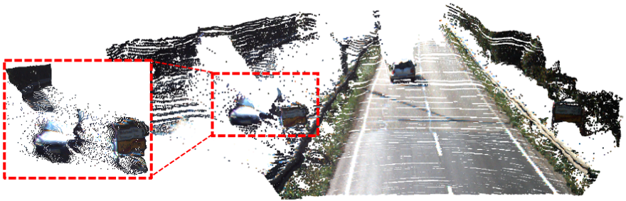
(a) PSMNet [5]

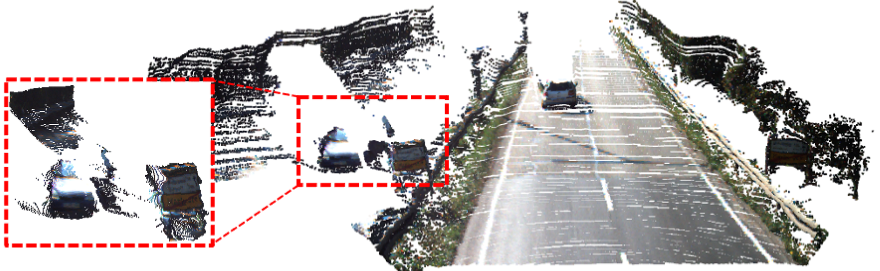
(b) PSMNet+[6]

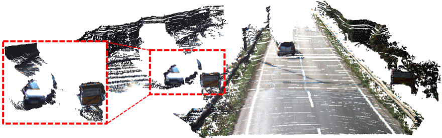
(c) PSMNet+Ours

Figure 1: Point clouds converted from disparity map on KITTI 2015 [7]. PSMNet [5] adopts Soft-Argmax [8] to estimate the disparity and suffers from over-smoothing problem. Single-modal disparity estimator in [6] alleviates this problem but many edge pixels are misaligned. Our adaptive multi-modal cross-entropy loss combined with our dominant-modal disparity estimator can effectively reduce bleeding artifacts and recover point cloud with sharp object boundary and complete structure. Please zoom in for more details.

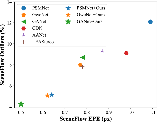
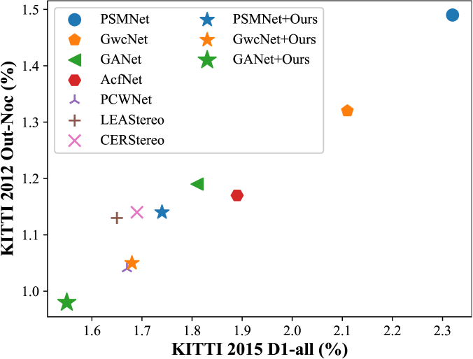
Figure 2: Performance comparison on the SceneFlow [9] and KITTI [10, 7] datasets. For all metrics, lower is better. Note that GANet [11] with our loss and disparity estimator achieves state-of-the-art performance.

Stereo matching is often regarded as a regression task in deep learning [8, 5, 12, 13]. The smooth L1 loss combined with the Soft-Argmax estimator [8] is usually employed to train the network and achieve sub-pixel disparity accuracy. However, smooth L1 loss lacks direct constraints on the cost volume, making it prone to overfitting during training [14]. Soft-Argmax is based on the assumption that the network outputs a uni-modal disparity distribution centered on the ground-truth [8], which is not always true especially for the edge pixels who have ambiguous depths. Applying Soft-Argmax on this non-unimodal distribution can cause serious over-smoothing problems [6], generating bleeding artifacts at the edge. As shown in Fig. 1(a), the space between the foreground objects (road signs, railings, vehicles) and the background (road, trees) is heavily polluted with flying points.

Another line of research treats stereo matching as a classification task and adopts cross-entropy as the loss function [15, 6, 14]. It provides direct supervision to the cost volume and can usually achieve better results than the regression method. Together with the disparity estimator based on single-modal weighted average [6], the over-smoothing problem can be effectively alleviated. However, the main problem with cross-entropy loss is that the ground-truth distribution for stereo matching is unavailable. Existing works adopt Laplacian or Gaussian distribution as the model and fit uni-modal distributions around the scalar ground-truth [15, 6, 14, 16]. Unfortunately, these uni-modal cross-entropy losses still tend to produce similar multi-modal distributions on the edge pixels, making it difficult to select out the correct peak for further processing. Enforcing single-modal disparity estimator on such ambiguous distributions may produce misalignment artifacts on the object boundaries, as shown in Fig. 1(b).

Our work aims to set up a better ground-truth distribution model for the cross-entropy loss and improve the disparity estimation. We first experimentally demonstrate that correct supervision at edges is challenging but important, as it affects the performance not only on edge pixels but also on non-edge pixels. In fact, since the intensity change of the edge pixels can be modeled as slopes, it is difficult to arbitrarily say whether they belong to the foreground or the background. Therefore, we argue that bi-modal distributions are more suitable for fitting the ground-truth at the edge. In addition, we should also take into account the relative height of the modals, which reflects the degree of difficulty in selecting the correct peak in the output distribution.

With these perceptions in mind, we further propose an adaptive multi-modal distribution for fitting the ground-truth in cross-entropy loss. We extract edge information from the neighborhood of each pixel to determine the number of modals in the distribution. Uni-modal and bi-modal distributions are fitted in the non-edge and edge regions, respectively. For bi-modal distributions, we extract structural information to adjust the relative height of the two modals. During inference, we refer to the single-modal weighted average operation [6], but determine the dominant modal by comparing the cumulative probabilities of the two modals. Additionally, the disparity distribution is filtered before scoping the dominant modal. With these significant improvements, the misalignment artifacts are largely reduced and a much more accurate disparity estimation can be obtained, as shown in Fig. 1(c).

Since November 2022, GANet [11] trained with our method achieves state-of-the-art performance on SceneFlow test set and ranks $1^{st}$ on both the KITTI 2015 [7] and KITTI 2012 [10] benchmarks, as shown in Fig. 2. Meanwhile, our method shows excellent cross-domain generalization ability and surpasses existing methods that specialize in generalization. We also conduct experiments on the impact of ground-truth density to the model performance, which is important for real-world outdoor stereo applications since only sparse LiDAR can be used as the ground-truth. Our model shows superior robustness than the baseline methods.

Our contributions are summarized as follows: (1) We experimentally demonstrate the importance of correct edge supervision to the stereo matching problem; (2) We propose an adaptive multi-modal cross-entropy loss for network training. It can effectively reduce the ambiguous output distributions; (3) We optimize the disparity estimator to obtain more robust disparity results during inference; (4) Classic models trained with our method can regain highly competitive performance; (5) Without any additional design on domain generalization, our method exhibits excellent synthetic-to-realistic cross-domain generalization.

II Related Work

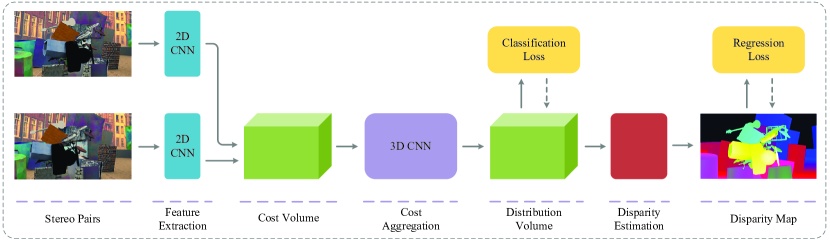
Figure 3: Typical architecture of the 3D-Conv stereo models. Cost volume is the 4D tensor whose feature dimension is omitted. Distribution volume is output by the cost aggregation module and then normalized by the Softmax operation. The regression loss supervises the disparity map while the classification loss directly supervises the distribution volume.

Deep Stereo Matching. Initially, researches on applying deep learning to stereo matching aim to improve particular steps in the traditional stereo pipeline [4], such as learning a matching cost function to replace a manually designed one [17, 18] or learning to improve subsequent optimization [19, 20] and refinement [21, 22]. These methods are not end-to-end and obtain limited accuracy gains. Later, Mayer et al. propose the first end-to-end training model DispNet and achieve performance boost [9]. Based on the DispNet [9], GCNet [8] preserves the feature dimension in the 4D cost volume and proposes employing 3D convolution to regularize it. PSMNet [5] further adds the spatial pyramid pooling layer [23] to take advantage of multi-scale information, and stacks multiple hourglass networks to improve the accuracy. GwcNet [12] adjusts the structure of the stacked hourglass network in PSMNet [5] and creatively constructs the cost volume by group-wise correlation which provides efficient representations for measuring feature similarities. To replace the 3D convolutional layers in the cost aggregation stage which have cubic computational/memory complexity, GANet [11] proposes the semi-global and local guided aggregation layers. The former is a differentiable approximation of the semi-global matching [24] and the latter follows a traditional cost filtering strategy [25] to refine thin structures. There are also some works that obtain the optimal network architecture through Neural Architecture Search (NAS), such as LEAStereo [26]. Recently, ACVNet [27] uses attention weights to suppress redundant information and enhance matching-related information in the concatenation volume.

Loss Function and Disparity Estimator. Loss function and disparity estimator are crucial for stereo networks. The former supervises the learning process of the network, and the latter finalizes the result from the disparity distribution output by the network. In GCNet [8], regression-based L1 loss is adopted and the full-band weighted average operation (Soft-Argmax) is proposed to calculate the final disparity. Later, smooth L1 loss becomes the mainstream [5, 12, 28, 13]. Different from the above works, PDSNet [15] uses the classification-based cross-entropy loss with Laplacian distribution to train the stereo model, and then single-modal weighted average operation is used to estimate the final disparity. Chen et al.  [6] adjust the range of the dominant modal dynamically through monotonicity to obtain more accurate estimation. AcfNet [14] leverages variances of the output distributions to explicitly model matching uncertainty and control the sharpness of the ground-truth distributions. CDN [29] utilizes a sub-network to estimate fractional biases for each integer disparity candidate and refers to the Wasserstein distance [30] as the loss function. By exploiting bi-modal mixture densities as output representation, SMDNet [31] minimizes the negative log-likelihood loss and is capable of predicting sharp boundaries around objects. Unlike these previous methods which all seek to suppress the production of multi-modal outputs, our method encourages the network to generate appropriate bi-modal distributions at the edge and then post-process them to achieve more accurate results.

Cross-Domain Generalization. As an important issue for all machine learning algorithms, cross-domain generalization is also intensively studied in stereo matching. DSMNet [32] proposes a novel domain normalization layer combined with a learnable non-local graph-based filtering layer to reduce the domain shifts. CFNet [33] builds a cascade and fused cost volume representation to learn domain-invariant geometric scene information. Other works hope to improve the generalization ability by extracting domain-invariant features from the stereo images. ITSA [34] refers to the information bottleneck principle [35, 36] to minimize the sensitivity of the feature representations to the domain variation. GraftNet [37] embeds a feature extractor pre-trained on large-scale datasets into the stereo matching network to extract broad-spectrum features. Our method improves the generalization performance by merely training the network with a superior loss function.

III Methodology

III-A Fundamentals and Problem Statement

TABLE I: The influence of edge supervision in cross-entropy loss on SceneFlow [9]. We use the strategy described in Section III-B to segment edge and non-edge pixels. Baseline: the uni-modal distribution is used as the ground-truth for all pixels. None Edge GT: edge pixels are not involved in the calculation of the loss. Noisy Edge GT: erroneous supervision is performed at the edge by adding random noise to the disparity ground-truth, and then the noisy disparity is used to fit the distribution. Noisy Global GT: erroneous supervision is distributed globally with the same percentage of edge pixels in the image.

Method	All			Edge			Non-Edge
	EPE	>1px	>3px	EPE	>1px	>3px	EPE	>1px	>3px
Baseline [6]	0.84	6.65	2.85	7.73	26.38	19.39	0.55	5.87	2.20
None Edge GT	0.89	6.89	2.95	8.86	30.34	22.25	0.55	5.95	2.18
Noisy Edge GT	1.14	8.03	3.58	15.50	48.71	36.46	0.56	6.43	2.27
Noisy Global GT	0.87	6.96	2.95	7.96	27.75	20.78	0.57	6.14	2.26

Given a calibrated stereo image pair, we want to find the corresponding pixel in the right image for each pixel in the left image. According to the convolution method used in the aggregation stage, the stereo models can be subdivided into two categories: 2D-Conv models [38, 39, 40, 41] and 3D-Conv models [28, 5, 12, 11]. The latter can usually achieve better results than the former, while at the cost of higher computational complexity. 3D-Conv models share a common pipeline [8], as shown in Fig. 3. First, features of the left and right images are extracted by a weight-sharing 2D CNN module respectively. Then the 4D cost volume is constructed upon the two obtained feature blocks. The cost aggregation module takes this 4D volume as input and outputs a $D\times H\times W$ volume, where $D$ is the maximum range of disparity search, $H$ and $W$ are the height and width of the input image, respectively. Softmax operation is then applied in the dimension $D$ to get the disparity distribution $p(\cdot)$. Finally, the disparity $\hat{d}$ with sub-pixel accuracy is estimated by the weighted average operation, which is also called the Soft-Argmax:

$$\hat{d}=\sum_{d=0}^{D-1}d\cdot p(d)$$ (1)

For the training of the stereo network, regression-based smooth L1 loss is usually employed, as:

$$L_{reg}(\hat{d},d_{gt})=\begin{cases}0.5(\hat{d}-d_{gt})^{2},&if\ |\hat{d}-d_{gt}|<1,\\ |\hat{d}-d_{gt}|-0.5,&otherwise.\\ \end{cases}$$ (2)

where $d_{gt}$ is the ground-truth disparity.

As shown in Fig. 3, the problem of smooth L1 loss is that the distribution volume is not directly supervised by the ground-truth, which can lead to some degree of overfitting during training [14]. Therefore, it is natural to explore more direct supervision on the distribution volume to alleviate this problem. By treating the stereo matching as a classification task, cross-entropy loss shown in Equation (3) is a good option for directly supervising the distribution volume:

$$L_{ce}(p,p_{gt})=-\sum_{d=0}^{D-1}p_{gt}(d)\cdot logp(d)$$ (3)

The new problem associated with the cross-entropy loss is that the ground-truth disparity is not an integer and its distribution $p_{gt}(\cdot)$ in Equation (3) is unavailable. Some works [15, 6, 14] use Gaussian or Laplacian model to transform the scalar ground-truth disparity into the discrete distribution. They directly generate uni-modal distribution around ground-truth for all pixels to meet the requirement of $p_{gt}(\cdot)$. However, this simple model seems not able to impose equal supervision to the pixels on the image. We separately record the training losses for edge and non-edge pixels on SceneFlow [9] and plot them in Fig. 4. We can see that the loss of edge pixels drops much slower and remains much larger than that of the non-edge pixels, which means that learning is much more difficult for the edge pixels than for the others. We attribute this to the inappropriate supervision at the edge. In fact, since the intensity change of the edge pixels can usually be modeled as slopes, it is difficult to arbitrarily say whether they belong to the foreground or the background. Simple uni-modal assumption on them can produce extra noises on ground-truth, which leads to larger training loss than those of clean samples. To check how much influence the noisy edge ground-truth could have on the final precision, we replace the edge ground-truth disparity with random noise generated by a even distribution on the entire disparity range, and compare it with the other configurations. As shown in Table I, removing the edge supervision during training only leads to a slight performance drop in edge and all regions. However, adding erroneous edge supervision to the network causes dramatic performance degradation for both edge and non-edge pixels, with EPE from 0.84px to 1.14px and 1px error from 6.65% to 8.03% for All pixels, respectively. While if we distribute the same percentage of noisy label over the entire image, the negative influence can be largely reduced. This experiment clearly shows the importance of the correct edge supervision to the final precision. It affects not only the accuracy of the edge pixels, but also the accuracy of the non-edge pixels. This surprising discovery inspires us to explore the better modeling of the ground-truth distribution at the edge.

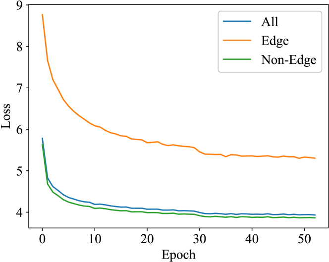
Figure 4: Training losses on the subset of SceneFlow dataset. The loss at the edge is much larger than that at the non-edge, which indicates that learning for the edge pixels is hard.

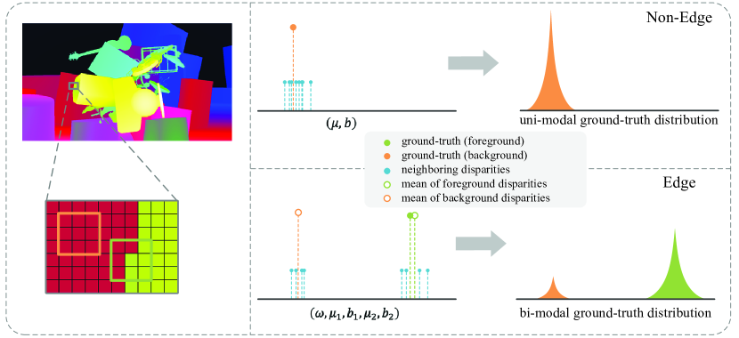
Figure 5: Our adaptive multi-modal ground-truth distribution for cross-entropy loss. The left column shows the input image with partial enlargement under it. Two neighborhoods with size $3\times 3$ centered on non-edge (orange) and edge (green) pixels respectively are taken as examples. The right column shows the different generated modal based on the statistic of the pixels within the neighborhoods. For the non-edge pixel, the uni-modal Laplacian distribution is generated. While for the edge pixel, the nine disparities within the neighborhood are clustered into two classes (background and foreground), which are subsequently used to generate the bi-modal Laplacian distribution.

III-B Adaptive Multi-Modal Cross-Entropy Loss

Arpit et al. point out that neural networks tend to learn simple and clear patterns preferentially [42]. For stereo matching, it is intuitively difficult to distinguish whether the pixels at the edge belong to the foreground or the background. On the one hand, the edge pixels are blurred to some degree because the photosensitive element receives the blended light from the foreground and background at the same time. On the other hand, the space resolution is usually reduced in the feature extraction stage of the stereo network, which further blurs the feature of the edge pixels. Therefore, we have reason to believe that the actual distribution of edge pixels should have at least two peaks instead of one, with each of them centered on the foreground and the background disparities, respectively.

To this end, we propose a method to generate multi-modal ground-truth distribution adaptively from the ground-truth disparity map. We extract both edge and structural information from the the neighborhood of each pixel. The former determines the number of modals in the distribution, and the latter determines the relative height between each modal. Fig. 5 illustrates the generation process of our distribution.

Specifically, we choose the neighborhood of size $m\times n$ centered on each pixel in the ground-truth disparity map. Then, we compute the mean disparity for these $mn$ pixels. If the difference between the mean value and the central disparity is within a threshold $\epsilon$, the pixel is considered to be in the non-edge region, otherwise it is regarded as an edge pixel. For the non-edge pixels, we consider the ground-truth distributions to be uni-modal and fit them with softmax formed Laplacian distributions, as:

$$p_{lap}(d)=\frac{e^{-\frac{|d-\mu|}{b}}}{\sum_{i=0}^{D-1}e^{-\frac{|i-\mu|}{b}}}$$ (4)

where the location parameter $\mu$ is set to the disparity ground-truth, and $b$ is the scale parameter. For edge pixels, we consider the ground-truth distributions to be bi-modal. Using more than two modals contributes little to the final results, as will be shown in the experimental section later.

For edge pixels, the disparities within the neighborhood can be easily divided into two clusters, due to the obvious disparity gap between the foreground and the background. Assuming that cluster $P_{1}$ contains the central pixel and $P_{2}$ is the rest cluster, we fit these clusters with a bi-modal Laplacian distribution, as:

$$p_{gt}(d)=w\cdot\frac{e^{-\frac{|d-\mu_{1}|}{b_{1}}}}{\sum\limits_{i=0}^{D-1}e^{-\frac{|i-\mu_{1}|}{b_{1}}}}+(1-w)\cdot\frac{e^{-\frac{|d-\mu_{2}|}{b_{2}}}}{\sum\limits_{i=0}^{D-1}e^{-\frac{|i-\mu_{2}|}{b_{2}}}}$$ (5)

In Equation (5), $\mu_{1}$, $\mu_{2}$ are the means of the disparities in $P_{1}$ and $P_{2}$, respectively, and $b_{1}$, $b_{2}$ are the scale parameters for controlling the sharpness of the modals. To ensure the accuracy of the dominant modal, $\mu_{1}$ is replaced by the central ground-truth disparity. The weight parameter $w$ is responsible for adjusting the relative height of the two modals according to the structural statistics. We take the number of pixels in $P_{1}$ as a indicator of the local structure. For example, smaller pixel quantity in $P_{1}$ corresponds to a thinner structure, which means we should lower the confidence of ground-truth accordingly. Finally, $w$ in Equation (5) is determined as:

$$w=\alpha+(|P_{1}|-1)\cdot\frac{1-\alpha}{mn-1}$$ (6)

where $|P_{1}|$ represents the number of pixels in $P_{1}$, $\alpha$ is the fixed weight for the central pixel, with the rest $(1-\alpha)$ weights equally distributed to the neighboring pixels. Equation (4) can be seen as a special case of Equation (5) when $|P_{1}|$ is equal to $mn$ and $P_{2}$ is empty.

III-C Dominant-Modal Disparity Estimator

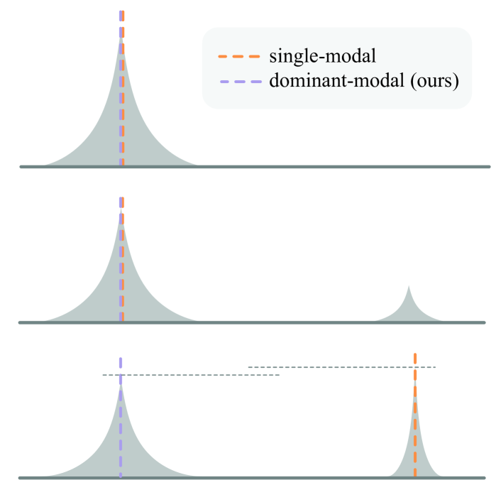
Figure 6: Three typical outputs from the network. From top to bottom: uni-modal distribution, easily distinguishable bi-modal distribution, ambiguous bi-modal distribution with similar peak height. For the third one, the single-modal disparity estimator [6] extracts the modal with the maximum probability candidate, while our dominant-modal estimator extracts the modal with greater cumulative probability.

The inferred disparity distributions tend to be consistent with the ground-truth distributions, which are the adaptive multi-modals in our work. Given the inferred distributions, we need to post-process them to obtain the final disparity results. Similar to Chen et al. [6], we estimate the result by performing a weighted average operation on the disparity candidates within the dominant modal. However, we differ from [6] in determining the range of the dominant modal. Chen et al. first locate the candidate disparity with the maximum probability, and then traverse left and right respectively until the probability no longer decreases, thereby determining the range of the dominant modal $[d_{l},d_{r}]$. However, when applying this method in the scenario of the ambiguous multi-modal distributions, as shown in Fig. 6, it is prone to locate the dominant peak incorrectly and produce disparity outliers. To avoid this problem, we propose a cumulative probability-based modal selection method. Specifically, we first adopt a mean filter to smooth the inferred disparity distribution. Then we compare the cumulative probabilities of the peaks and locate the largest one as the dominant peak. Next, we normalize the distribution of the dominant peak as:

$$\overline{p}(d)=\begin{cases}\frac{p(d)}{\sum_{i=d_{l}}^{d_{r}}p(i)},&if\ d_{l}\leq d\leq d_{r},\\ 0,&otherwise.\\ \end{cases}$$ (7)

Note that the normalization is carried out on the peak of raw output distribution $p(\cdot)$ rather than the smoothed one to preserve the accuracy of the disparity estimation. At last, the weighted average operation on the selected dominant modal is used to yield the final disparity from $\overline{p}(\cdot)$. The output difference between [6] and our method is illustrated in Fig. 6.

IV Experiments

IV-A Datasets and Evaluation Metrics

We evaluate our method on five popular stereo matching datasets.

SceneFlow [9] is a large synthetic dataset containing 35454 image pairs for training and 4370 for testing. The resolution of each image is 540×960 and it contains dense ground-truth disparity for training.

KITTI 2012 [10] is the dataset composed of images collected from outdoor driving scenes. It contains 389 pairs of images, of which 194 are used for training and 195 for testing. The ground-truth disparity is sparse since it is obtained by 3D LiDAR.

KITTI 2015 [7] is another dataset in KITTI, containing images in real driving scenes. It includes 200 training pairs and 200 testing pairs. We split 20 training pairs as the validation set, following [12]. Compared with KITTI 2012, KITTI 2015 takes further advantage of detailed 3D CAD models to recover ground-truth disparity on dynamic objects. For both KITTI 2012 and 2015, only the ground-truth of the training set is available, and the test results is submitted to the benchmark for evaluation and ranking.

Middlebury [43] is a real-world indoor dataset. It contains 15 training and 15 testing image pairs with dense labeled ground-truth. We use the half resolution of the training set to evaluate the cross-domain generalization performance.

ETH3D [44] is a dataset of indoor and outdoor scenes, providing 27 low-res two-view image pairs for training and 20 for testing. We compare the generalization ability of our method with other works on the training set.

For SceneFlow, end-point error (EPE) and $k$px error are used to evaluate the performance of the model. The former reflects the overall performance and the latter represents the percentage of outliers with an absolute error greater than $k$ pixels. On KITTI 2015, a pixel is considered to be correctly estimated if the disparity error is less than 3px or 5%. The percentage of disparity outliers (D1) is evaluated for background, foreground, and all pixels. On KITTI 2012, percentages of erroneous pixels for both non-occluded (Noc) and all (All) pixels are reported. Similar $k$px metrics for non-occluded pixels are also used on Middlebury and ETH3D datasets.

IV-B Implementation Details

We apply the proposed loss function to some classic stereo models, such as PSMNet [5], GwcNet [12], and GANet [11]. We implement all models in PyTorch and use Adam with $\beta_{1}=0.9$ and $\beta_{2}=0.999$ as optimizer. We train the models from scratch using two NVIDIA 3090 GPUs. When training on SceneFlow [9], the initial learning rate is set to $1\times 10^{-3}$ for 30 epochs and then reduced to $1\times 10^{-4}$ for the rest 15 epochs. When fine-tuning the SceneFlow pre-trained model on the target datasets [10, 7], we use 600, 200 and 100 epochs with the learning rate $1\times 10^{-3}$, $1\times 10^{-4}$ and $1\times 10^{-5}$, respectively. The disparity threshold $\epsilon$ for determining edge or non-edge pixels is set to 5. All scale parameters in Laplacian distributions are set to 0.8. $\alpha$ in Equation (6) is set to 0.8 to guarantee the dominance of the modal with disparity ground-truth.

IV-C Ablation Study

In this section, we perform ablation experiments to evaluate the effectiveness of our method.

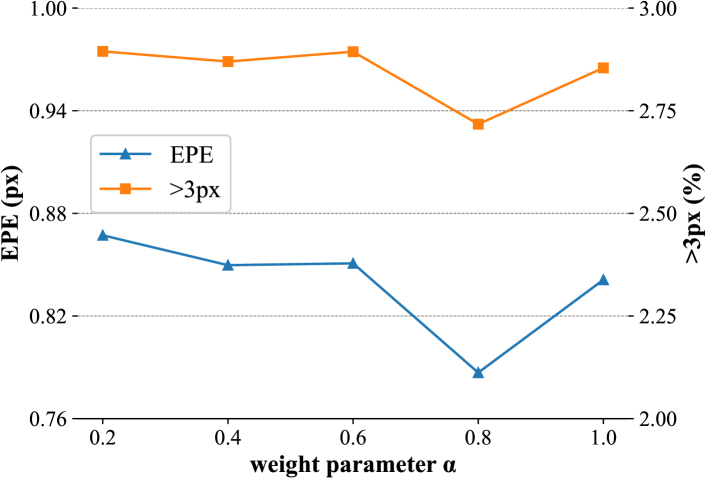
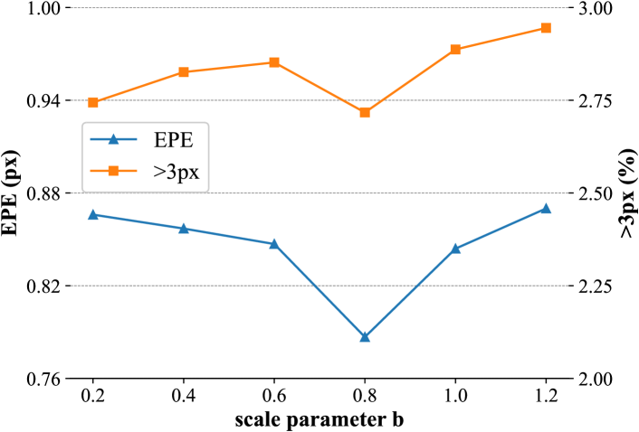
Figure 7: Determination of the hyper-parameters in our adaptive multi-modal cross-entropy loss, where weight parameter $\alpha$ controls the relative height of modals and scale parameter $b$ controls the width of the modals. The experiment is carried out on the SceneFlow dataset.

TABLE II: Ablation study of neighborhood shape and size on SceneFlow dataset. Uni-modal cross-entropy loss can be seen as a special case of ours, with the size of neighborhood is $1\times 1$. All methods are trained for 15 epochs from scratch.

Neighborhood Size	EPE	>1px	>3px
PSMNet [5]	0.97	10.51	4.03
$1\times 1$ [6]	0.84	6.65	2.85
$1\times 3$	0.82	6.76	2.85
$1\times 5$	0.81	6.58	2.79
$1\times 7$	0.81	6.62	2.83
$1\times 9$	0.78	6.30	2.71
$1\times 11$	0.84	6.72	2.91
$3\times 3$	0.83	6.67	2.86
$5\times 5$	0.82	6.42	2.79
$7\times 7$	0.92	6.63	2.98

TABLE III: Ablation study of the neighborhood size on KITTI 2015 validation set. All methods are trained for 400 epochs from scratch.

Neighborhood Size	EPE	D1
PSMNet [5]	0.68	1.90
$1\times 1$ [6]	0.67	1.77
$1\times 9$	0.67	1.64
$3\times 9$	0.65	1.58
$5\times 9$	0.68	1.84

Neighborhood Shape and Size. Edge and structural information within the neighborhood are extracted to fit the ground-truth distribution. We ablate to determine the optimal neighborhood shape and size in Table II. The two baselines are the PSMNets trained by smooth L1 loss [5] and uni-modal cross-entropy loss [6], respectively. The latter can be seen as a special case of ours, with the size of neighborhood $1\times 1$. From Table II, we find that the neighborhood size $1\times 9$ achieves the best result on SceneFlow dataset. Compared with the smooth L1 loss, we boost EPE by 19.59%, 1px error by 40.06%, and 3px error by 32.75%. Compared with the uni-modal cross-entropy loss, the proposed adaptive multi-modal cross-entropy loss leads on all metrics. Meanwhile, neighborhoods with 1D shapes usually perform better than those with 2D shapes. This may attributed to the fact that stereo matching is a 1D matching task along horizontal scan lines. When fine-tuning the pre-trained model on the KITTI datasets, leveraging the adjacent rows to extract more structural information could be beneficial, as the ground-truth of KITTI is sparse [10, 7]. As shown in Table III, the neighborhood of size $3\times 9$ achieves the best result on KITTI 2015.

TABLE IV: Ablation study of disparity estimator on SceneFlow. SM: single-modal weighted average operation; DM: our dominant-modal weighted average operation. Our DM disparity estimator achieves better results than SM for both uni-modal cross-entropy loss and our adaptive multi-modal cross-entropy loss. The best result is shown in bold and the second-best result is underlined.

Loss	Estimator	EPE	>1px	>3px
Uni-Modal Cross-Entropy	Argmax	1.39	37.36	2.98
	Soft-Argmax [8]	0.96	10.29	5.18
	SM [6]	0.84	6.65	2.85
	DM	0.82	6.61	2.82
Adaptive Multi-Modal Cross-Entropy	Argmax	1.33	35.98	2.87
	Soft-Argmax [8]	0.92	9.77	4.97
	SM [6]	0.80	6.31	2.72
	DM	0.78	6.30	2.71

Disparity Estimator. We perform ablations on the different disparity estimators in Table IV. For both cases of uni-modal and our multi-modal loss, disparity estimator with simple Argmax performs the worst. This is due to the fact that Argmax just take the integer candidate disparity with the highest probability as the final result, which is not robust to the outliers with small threshold. Soft-Argmax [8] can obtain much better results than Argmax, thanks to its ability to aggregate the probability along the entire disparity dimension. Taking only the peak with the highest probability into account, the single-modal estimator [6] can further reduce the proportion of outliers upon Soft-Argmax. Finally, by better locating the range of the dominant peak, our dominant-modal estimator achieves the best performance among the listed methods. On the other hand, comparing with the uni-modal cross-entropy loss, our adaptive multi-modal loss with single-modal disparity estimator [6] also performs much better on all of the metrics, which clearly reveals the effectiveness of our proposed loss. Combining our loss with the dominant-modal estimator together can further improve the performance.

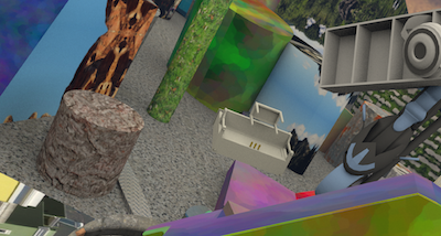
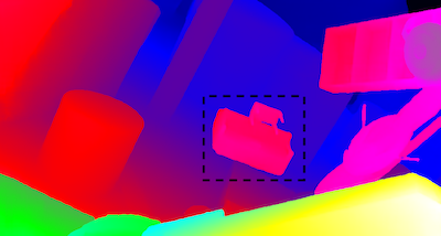
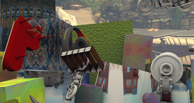
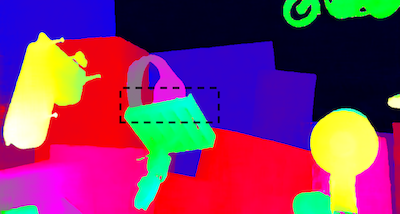
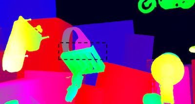
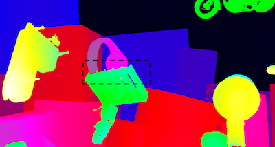
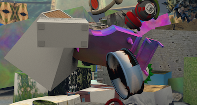
(a) Left Image

(b) PSMNet [5]

(c) PSMNet+[6]

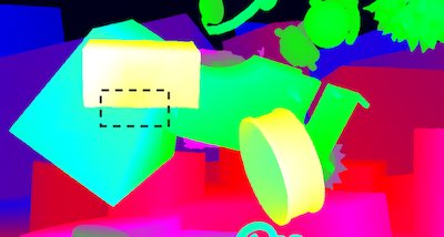
(d) PSMNet+Ours

Figure 8: Qualitative comparison on Scene Flow. By learning appropriate patterns at the edge, we can obtain clear and sharp edges in the final disparity map. Please zoom in for more details.

TABLE V: Results on SceneFlow. The best result is shown in bold and the second-best result is underlined.

Method	EPE	>1px	>3px
MC-CNN[45]	3.79	–	13.7
GCNet[8]	2.51	16.9	9.34
PSMNet[5]	1.09	12.1	4.56
CDN[29]	0.98	9.10	3.99
AANet[46]	0.87	9.30	–
AcfNet[14]	0.87	–	4.31
GANet[11]	0.78	8.70	–
LEAStereo[26]	0.78	7.82	–
GwcNet[12]	0.77	8.00	3.30
PSMNet+[6]	0.77	–	2.21
EDNet[41]	0.63	–	–
PSMNet+Ours	0.64	5.14	2.19
GwcNet+Ours	0.62	5.07	2.16
GANet+Ours	0.50	4.25	1.81

Weight and Scale Parameters. Fig. 7 shows the experiment of selecting optimal value for the hyper-parameters in our distribution model. The weight parameter $\alpha$ in Equation (6) determines the relative height between foreground and background modals. When $\alpha$ is set to one, the bi-modal distribution degenerates into the uni-modal distribution. If $\alpha$ is too small, the dominant ground-truth peak will become too small and make it hard for the network to learn and output correct distribution. The scale parameter $b$ controls the sharpness of the distribution, which has a great influence on the final performance. Through the experimental result in Fig. 7, setting both $\alpha$ and $b$ to 0.8 is optimal.

IV-D Performance Evaluation

SceneFlow. We compare our method with published methods on SceneFlow test set [9]. We use PSMNet [5], GwcNet [12], and GANet [11], which are originally trained by smooth L1 loss, as our baseline models for the evaluation. As shown in Table V, our method can greatly improve the performance of all of the baselines by simply changing the training loss and the post-processing disparity estimator. In particular, the EPE are improved by 41.28%, 19.48% and 35.90% on the baselines PSMNet, GwcNet, and GANet, respectively. The 1px and 3px error are also improved by at least 36.63% and 34.55%, respectively. GANet [11] trained by our loss outperforms previous state-of-the-art results and achieves the best performance. Our models also perform much better than [6], which employs uni-modal cross-entropy loss to train the PSMNet [5] and uses single-modal disparity estimator in inference. The promising results in Table V strongly demonstrate the effectiveness of our method in promoting the performance of existing models. Fig. 8 qualitatively shows the results of the disparity estimation on SceneFlow. Our method can recover more accurate object structure and reduce undesired defects at the edge of objects.

KITTI 2015 & KITTI 2012. We submit our results to the KITTI 2015 [7] and KITTI 2012 [10] benchmarks for further comparison with other methods, and the results are listed in Table VI. As expected, all of the three baseline models are lifted to a highly competitive level by our method. In particular, GANet [11] trained by our method achieves new state-of-the-art results on both KITTI 2015 and KITTI 2012 benchmarks. Up to now, most models can only achieve the state-of-the-art result on one of these two datasets, even the domain gap between them is relatively small. This shows the superior robustness of our method. More experiments on the cross-domain generalization will be shown in Section IV-F.

TABLE VI: Results on KITTI 2015 and KITTI 2012 Benchmarks. * means that the loss function of this method contains a uni-modal cross-entropy loss term. The best result is shown in bold and the second-best result is underlined.

Method	KITTI 2015						KITTI 2012
	All			Noc			>2px		>3px
	D1-bg	D1-fg	D1-all	D1-bg	D1-fg	D1-all	Out-Noc	Out-All	Out-Noc	Out-All
GCNet [8]	2.21	6.16	2.87	2.02	5.58	2.61	2.71	3.46	1.77	2.30
PDSNet [15]	2.29	4.05	2.58	2.09	3.68	2.36	3.82	4.65	1.92	2.53
PSMNet [5]	1.86	4.62	2.32	1.71	4.31	2.14	2.44	3.01	1.49	1.89
PSMNet+[6]	1.54	4.33	2.14	1.70	3.90	1.93	2.17	2.81	1.35	1.81
GwcNet [12]	1.74	3.93	2.11	1.61	3.49	1.92	2.16	2.71	1.32	1.70
SMDNet [6]	1.69	4.01	2.08	1.54	3.70	1.89	–	–	–	–
AcfNet [14]	1.51	3.80	1.89	1.43	3.25	1.73	1.83	2.35	1.17	1.54
GANet [11]	1.48	3.46	1.81	1.34	3.11	1.63	1.89	2.50	1.19	1.60
GANet+LaC [16]	1.44	2.83	1.67	1.26	2.64	1.49	1.72	2.26	1.05	1.42
PCWNet [47]	1.37	3.16	1.67	1.26	2.93	1.53	1.69	2.18	1.04	1.37
ACVNet [27]	1.37	3.07	1.65	1.26	2.84	1.52	1.83	2.34	1.13	1.47
LEAStereo [26]	1.40	2.91	1.65	1.29	2.65	1.51	1.90	2.39	1.13	1.45
PSMNet+Ours	1.44	3.25	1.74	1.30	3.04	1.59	1.80	2.32	1.14	1.50
GwcNet+Ours	1.42	3.01	1.68	1.30	2.76	1.54	1.65	2.17	1.05	1.42
GANet+Ours	1.38	2.40	1.55	1.25	2.19	1.41	1.52	2.01	0.98	1.29

To more intuitively show our improvement in edge quality, we convert the disparity maps to point clouds and plot the corresponding error maps in Fig. 10. Our method dramatically improves the bleeding artifacts, and obtains point cloud with clear object boundaries, which is beneficial when applying the reconstructed point cloud in downstream robotic tasks such as 3D object detection.

IV-E Analysis of the Real Output Distribution Patterns

In this section, we analyze the real output distribution patterns produced by different loss functions and give more discussion on them.

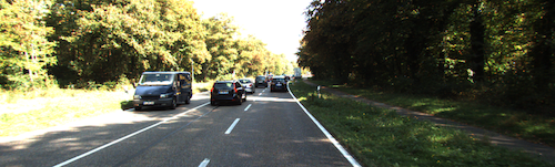
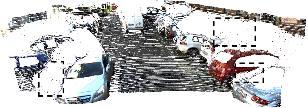
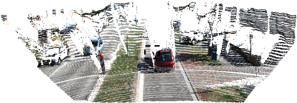
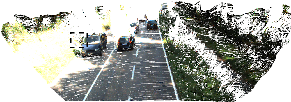
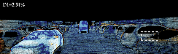
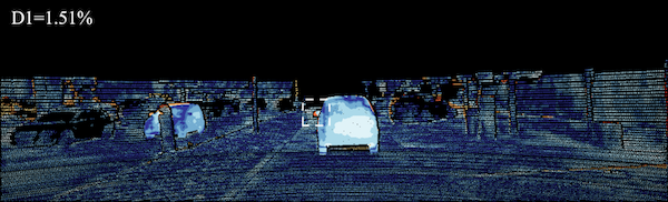
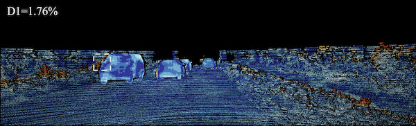
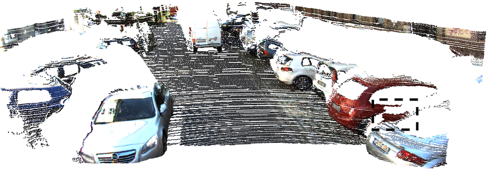
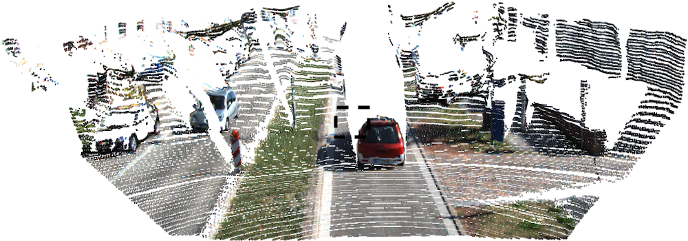
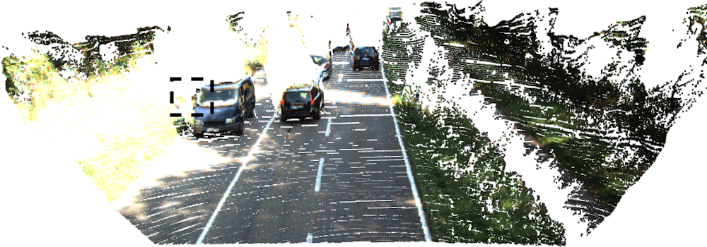
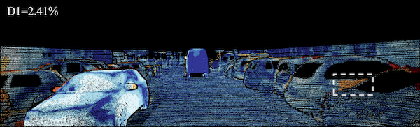
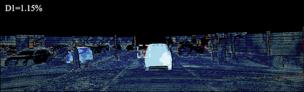
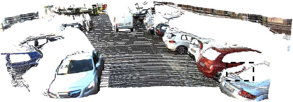
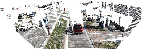
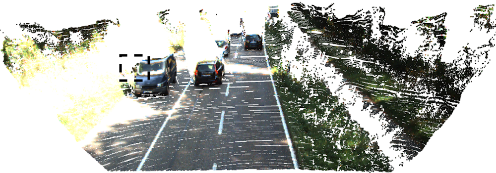
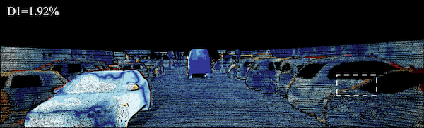
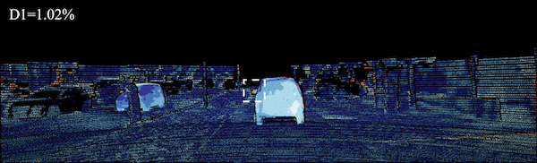
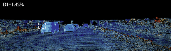
Figure 9: Comparison of point cloud quality on KITTI 2015 validation set. From top to bottom: left image, point clouds and error maps of PSMNet [5], point clouds and error maps of PSMNet+[6], point clouds and error maps of PSMNet+Ours. The dashed boxes mark some of the bleeding and misalignment artifacts which are noticeable in [5] and in [6]. Please zoom in for more details.

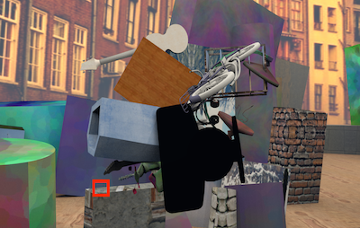
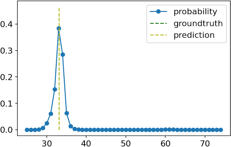
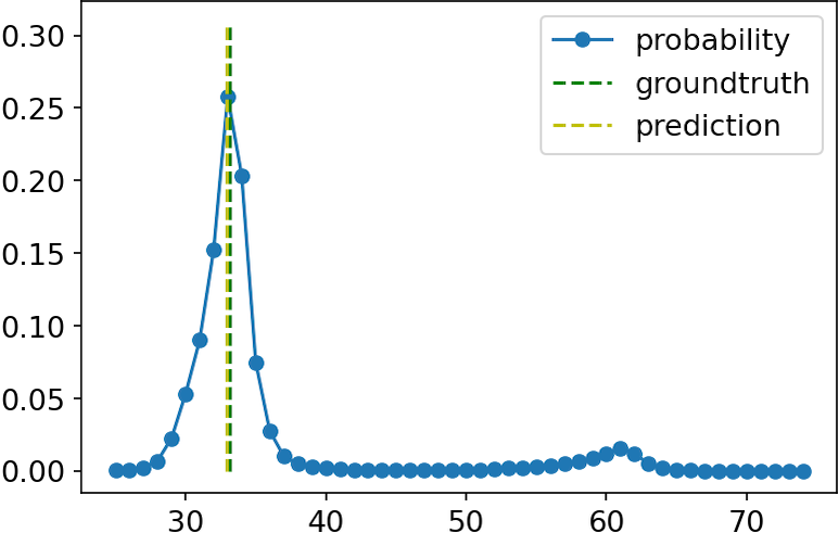
(a) Left Image

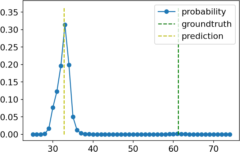
(b) PSMNet [5]

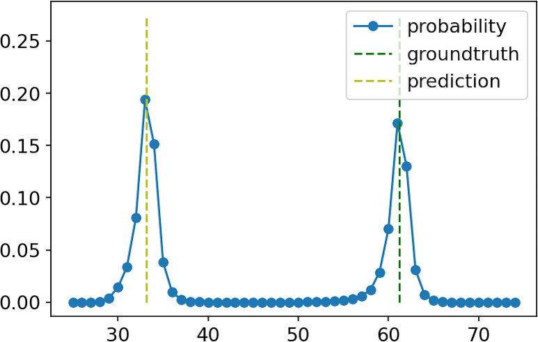
(c) PSMNet+[6]

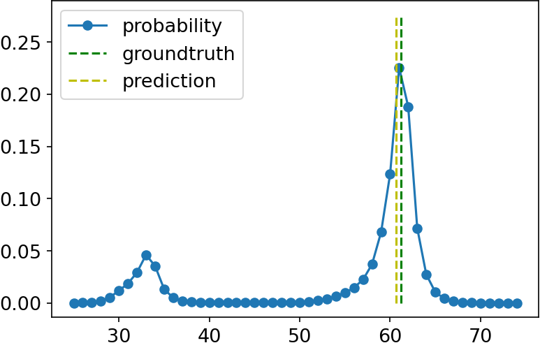
(d) PSMNet+Ours

Figure 10: Visualization of the real output distributions at the edge pixels on SceneFlow dataset. (a): The scene image, and its partial enlargement. The edge pixels marked green and yellow belong to the background and foreground with different depth, respectively. (b), (c), and (d) show the output probability distributions from PSMNet [5], PSMNet+[6], and PSMNet+Ours. The first row corresponds to the green pixel and the second row corresponds to the yellow pixel. Our method can produce distinguishable probability peaks and obtain correct disparity estimation. Please zoom in to see the details.

TABLE VII: Output modal number and outlier (>3px) statistics of PSMNet [5] trained by different loss functions on SceneFlow. We use the strategy described in Section III-B to segment edge and non-edge regions. Modals with the maximum value lower than 1% are not included in the statistics. Note that our adaptive multi-modal cross-entropy loss outputs more multi-modal distributions than the uni-modal cross-entropy loss at the edge, while the opposite is true at the non-edge.

Loss	Region	The proportion of #modal (%)			Outliers (%)
		1	2	Others
Smooth L1	All	98.50	1.00	0.50	4.03
	Edge	87.79	10.30	1.91	25.59
	Non-Edge	98.92	0.64	0.44	3.17
Uni-Modal Cross-Entropy	All	94.67	4.60	0.73	2.85
	Edge	40.16	52.70	7.14	19.39
	Non-Edge	96.78	2.77	0.45	2.20
Adaptive Multi-Modal Cross-Entropy (Ours)	All	94.92	4.35	0.73	2.71
	Edge	35.35	57.28	7.37	18.97
	Non-Edge	97.23	2.33	0.44	2.07

Fig. 10 visualizes the output distributions at some edge pixels for qualitative comparison. Although PSMNet [5] seldom produces bi-modal distributions for all pixels, it mistakenly estimates the foreground pixel (the yellow one) as the background. The method of Chen et al.  [6] outputs a uni-modal distribution for the background pixel but a bi-modal distribution for the foreground pixel. This means that the uni-modal cross-entropy loss cannot completely avoid producing distributions with more than one modal. Chen et al. hope to solve this problem by single-modal disparity estimator [6]. Unfortunately, in this case the background peak is slightly higher, causing the yellow pixel to be mistakenly estimated as the background. As expected, PSMNet trained by our adaptive multi-modal cross-entropy loss yields bi-modal distributions for edge pixels. The two peaks in the bi-modal pattern are easily distinguishable, with the correct disparity on the dominant peak, as shown in Fig. 10(d). This should thank to the adaptive weighting mechanism used in generating the ground-truth distribution, which can dynamically adjust the relative height of the two modals and ensure that the modal with disparity ground-truth always dominates.

We further count the proportions of pixels with different output modals and the corresponding outliers in Table VII. PSMNet [5] trained by smooth L1 loss yields the most uni-modal distributions at the edge, namely, 87.79%. However, a part of these uni-modal distributions may not be that certain, as they may centered at wrong disparities, as shown in Fig. 10(b). The proportion of multi-modal distributions in the edge regions rises from 12.21% (10.30%+1.91%) to 59.84% (52.70%+7.14%) when uni-modal cross-entropy loss [6] is employed, indicating the failure of the uni-modal constraint on the distribution volume. Comparing with the uni-modal loss, our adaptive multi-modal loss yields about 5 percent more multi-modals on the edge pixels while producing less 3px outliers. This demonstrates the superiority of our loss in supervising the model to produce easily distinguishable patterns for disparity estimation. Moreover, our model also achieve better non-edge performance than the uni-modal, with the 3px outlier decreased from 2.20% to 2.07%. This is consistent with our previous discovery in Section III-A, i.e. the quality of the edge supervision affects not only the edge but also the non-edge performance. Our adaptive multi-modal distribution with dynamic peak height is closer to the true distribution of edge pixels than the uni-modal.

IV-F Cross-Domain Generalization Evaluation

Besides the fine-tuning performance, the generalization to different domains is also very important for the pre-trained models which are planned to deploy in different real-world scenes. In this section, we compare the cross-domain generalization performance of our method with the baselines [5, 12, 11] and the state-of-the-art methods that are specially designed for cross-domain applications [32, 33, 48, 37, 34]. All the methods are trained only on SceneFlow training set and then tested on KITTI 2015 [7], KITTI 2012 [10], Middlebury(Half) [43], and ETH3D [44] training sets for a fair comparison.

As shown in Table VIII, the generalization performance of the baselines [5, 12, 11] can be greatly enhanced by deploying our method. Yang et al. propose that asymmetric augmentation can improve the generalization ability of the models [49]. Subsequent works follow this strategy and strive to obtain domain-invariant features in the feature extraction stage [48, 37, 34]. Our method surpasses existing works on all four datasets without changing the structures of the backbones or using extra asymmetric data augmentation. Compared with the existing best performance, we improve the outlier metric by 5.96%, 7.14%, 13.37%, and 55.69% on KITTI 2015, KITTI 2012, Middlebury, and ETH3D datasets, respectively. Fig.11 shows some qualitative results of PSMNet [5] and our method on the four datasets.

TABLE VIII: Cross-domain generalization evaluation. $k$px outliers are reported. * means that the asymmetric data augmentation strategy is leveraged during training.

Method	KT 15	KT 12	MB	ETH3D
	>3px	>3px	>2px	>1px
PSMNet [5]	16.3	15.1	25.1	23.8
GwcNet [12]	12.2	12.0	24.1	11.0
GANet [11]	11.7	10.1	20.3	14.1
DSMNet [32]	6.5	6.2	13.8	6.2
CFNet [33]	5.8	4.7	19.5	5.8
FC-GANet [48]	5.3	4.6	10.2	5.8
Graft-GANet [37]	4.9	4.2	9.8	6.2
PCWNet [47]	5.6	4.2	15.8	5.2
ITSA-CFNet [34]	4.7	4.2	10.4	5.1
PSMNet+Ours	4.70	4.12	8.68	3.15
GwcNet+Ours	4.42	4.11	8.96	3.21
GANet+Ours	4.68	3.90	8.49	2.26

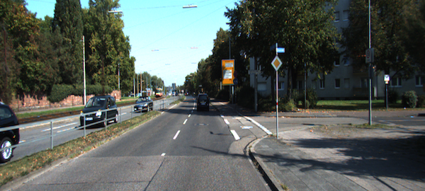
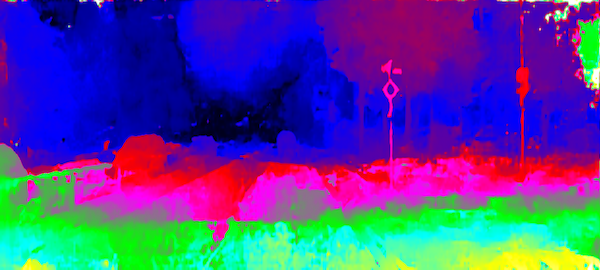
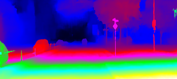
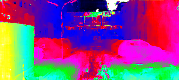
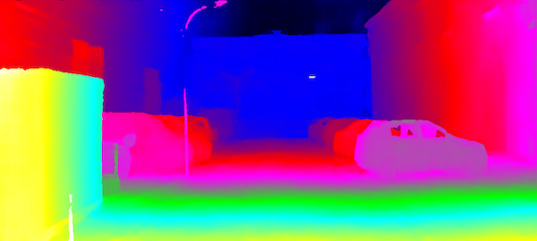
(a) Left Image

(b) PSMNet [5]

(c) PSMNet+Ours

Figure 11: Qualitative comparison of cross-domain generalization. Models are only trained on SceneFlow synthetic dataset [9] and tested on the four popular real-world datasets. From top to bottom: KITTI 2015 [7], KITTI 2012 [10], Middlebury [43], and ETH3D [44].

IV-G Influence of Ground-Truth Density

Most data-driven based stereo matching methods rely on full supervision for training. However, acquiring dense and accurate ground-truth for training could be difficult and expensive, especially for outdoor scenes. KITTI 2012 registers consecutive LiDAR point clouds with ICP to increase the ground-truth density [10], and KITTI 2015 further leverages detailed 3D CAD models to recover points on dynamic objects [7]. Through these measures, the overall average ground-truth density of KITTI 2015 is just about 19%, let alone the extra errors induced to the ground-truth during the point clouds registration. Therefore, a network that can be trained with sparser LiDAR ground-truth is highly desired.

In this experiment, we simulate different density of ground-truth by randomly down-sampling the original ground-truth on KITTI 2015, and then use them to train the network. Table IX lists the influence of the ground-truth density to the final performance. As expected, the performance of both methods degrades as the density of ground-truth decreases. However, our method is much less affected by the density reduction than its counterpart, with just about 10 percent degradation when trained with only 20% original ground-truth density. Even with this worst result, it is still much better than the best result of PSMNet trained with 100% original density. This clearly shows that the model with our method is robust to the ground-truth density, indicating the large potential to save the cost of data annotation in real application.

TABLE IX: Influence of the ground-truth density on KITTI 2015 validation set. Density represents the sampling percentage of the ground-truth used for training. D1 metric as well as its degradation percentage is reported.

Density	PSMNet [5]		PSMNet+Ours
	D1	Degradation	D1	Degradation
100%	1.90	–	1.58	–
80%	2.15	13.16%	1.61	1.90%
60%	2.24	17.89%	1.68	6.33%
40%	2.30	21.05%	1.71	8.23%
20%	2.35	23.68%	1.74	10.13%

V Conclusion

In this work, we discover the importance of correct edge supervision to stereo matching and propose a novel adaptive multi-modal cross-entropy loss for training the network. Our method is able to adaptively determine the number of modals and their relative height on the fitted distribution based on the statistics upon the local neighborhood, thereby provides better supervision for the edge pixels. We also optimize the disparity estimator to locate the dominant modal robustly. Our method can be easily applied to most of the existing stereo models. Extensive experiments have been carried out on several popular datasets. The results show that our method can boost the performance of existing models and the GANet trained by our method achieves the new state-of-the-art on the KITTI 2012 and 2015 benchmarks. Our method is also robust to the ground-truth density and has excellent cross-domain generalization performance.

References

- [1] S. Sivaraman and M. M. Trivedi, “A review of recent developments in vision-based vehicle detection,” in 2013 IEEE Intelligent Vehicles Symposium (IV). IEEE, 2013, pp. 310–315.
- [2] N. Zenati and N. Zerhouni, “Dense stereo matching with application to augmented reality,” in 2007 IEEE International Conference on Signal Processing and Communications. IEEE, 2007, pp. 1503–1506.
- [3] K. Schmid, T. Tomic, F. Ruess, H. Hirschmüller, and M. Suppa, “Stereo vision based indoor/outdoor navigation for flying robots,” in 2013 IEEE/RSJ international conference on intelligent robots and systems. IEEE, 2013, pp. 3955–3962.
- [4] D. Scharstein and R. Szeliski, “A taxonomy and evaluation of dense two-frame stereo correspondence algorithms,” International journal of computer vision, vol. 47, no. 1, pp. 7–42, 2002.
- [5] J.-R. Chang and Y.-S. Chen, “Pyramid stereo matching network,” in Proceedings of the IEEE conference on computer vision and pattern recognition, 2018, pp. 5410–5418.
- [6] C. Chen, X. Chen, and H. Cheng, “On the over-smoothing problem of cnn based disparity estimation,” in Proceedings of the IEEE/CVF International Conference on Computer Vision, 2019, pp. 8997–9005.
- [7] M. Menze and A. Geiger, “Object scene flow for autonomous vehicles,” in Proceedings of the IEEE conference on computer vision and pattern recognition, 2015, pp. 3061–3070.
- [8] A. Kendall, H. Martirosyan, S. Dasgupta, P. Henry, R. Kennedy, A. Bachrach, and A. Bry, “End-to-end learning of geometry and context for deep stereo regression,” in Proceedings of the IEEE international conference on computer vision, 2017, pp. 66–75.
- [9] N. Mayer, E. Ilg, P. Hausser, P. Fischer, D. Cremers, A. Dosovitskiy, and T. Brox, “A large dataset to train convolutional networks for disparity, optical flow, and scene flow estimation,” in Proceedings of the IEEE conference on computer vision and pattern recognition, 2016, pp. 4040–4048.
- [10] A. Geiger, P. Lenz, and R. Urtasun, “Are we ready for autonomous driving? the kitti vision benchmark suite,” in 2012 IEEE conference on computer vision and pattern recognition. IEEE, 2012, pp. 3354–3361.
- [11] F. Zhang, V. Prisacariu, R. Yang, and P. H. Torr, “Ga-net: Guided aggregation net for end-to-end stereo matching,” in Proceedings of the IEEE/CVF Conference on Computer Vision and Pattern Recognition, 2019, pp. 185–194.
- [12] X. Guo, K. Yang, W. Yang, X. Wang, and H. Li, “Group-wise correlation stereo network,” in Proceedings of the IEEE/CVF Conference on Computer Vision and Pattern Recognition, 2019, pp. 3273–3282.
- [13] S. Chen, Z. Xiang, C. Qiao, Y. Chen, and T. Bai, “Sgnet: Semantics guided deep stereo matching,” in Proceedings of the Asian Conference on Computer Vision, 2020.
- [14] Y. Zhang, Y. Chen, X. Bai, S. Yu, K. Yu, Z. Li, and K. Yang, “Adaptive unimodal cost volume filtering for deep stereo matching,” in Proceedings of the AAAI Conference on Artificial Intelligence, vol. 34, no. 07, 2020, pp. 12 926–12 934.
- [15] S. Tulyakov, A. Ivanov, and F. Fleuret, “Practical deep stereo (pds): Toward applications-friendly deep stereo matching,” Advances in neural information processing systems, vol. 31, 2018.
- [16] B. Liu, H. Yu, and Y. Long, “Local similarity pattern and cost self-reassembling for deep stereo matching networks,” in Proceedings of the AAAI Conference on Artificial Intelligence, vol. 36, no. 2, 2022, pp. 1647–1655.
- [17] J. Zbontar, Y. LeCun et al., “Stereo matching by training a convolutional neural network to compare image patches.” J. Mach. Learn. Res., vol. 17, no. 1, pp. 2287–2318, 2016.
- [18] W. Luo, A. G. Schwing, and R. Urtasun, “Efficient deep learning for stereo matching,” in Proceedings of the IEEE conference on computer vision and pattern recognition, 2016, pp. 5695–5703.
- [19] A. Seki and M. Pollefeys, “Patch based confidence prediction for dense disparity map.” in BMVC, vol. 2, no. 3, 2016, p. 4.
- [20] ——, “Sgm-nets: Semi-global matching with neural networks,” in Proceedings of the IEEE conference on computer vision and pattern recognition, 2017, pp. 231–240.
- [21] A. Shaked and L. Wolf, “Improved stereo matching with constant highway networks and reflective confidence learning,” in Proceedings of the IEEE conference on computer vision and pattern recognition, 2017, pp. 4641–4650.
- [22] S. Gidaris and N. Komodakis, “Detect, replace, refine: Deep structured prediction for pixel wise labeling,” in Proceedings of the IEEE conference on computer vision and pattern recognition, 2017, pp. 5248–5257.
- [23] K. He, X. Zhang, S. Ren, and J. Sun, “Spatial pyramid pooling in deep convolutional networks for visual recognition,” IEEE transactions on pattern analysis and machine intelligence, vol. 37, no. 9, pp. 1904–1916, 2015.
- [24] H. Hirschmuller, “Stereo processing by semiglobal matching and mutual information,” IEEE Transactions on pattern analysis and machine intelligence, vol. 30, no. 2, pp. 328–341, 2007.
- [25] A. Hosni, C. Rhemann, M. Bleyer, C. Rother, and M. Gelautz, “Fast cost-volume filtering for visual correspondence and beyond,” IEEE transactions on pattern analysis and machine intelligence, vol. 35, no. 2, pp. 504–511, 2012.
- [26] X. Cheng, Y. Zhong, M. Harandi, Y. Dai, X. Chang, H. Li, T. Drummond, and Z. Ge, “Hierarchical neural architecture search for deep stereo matching,” Advances in Neural Information Processing Systems, vol. 33, pp. 22 158–22 169, 2020.
- [27] G. Xu, J. Cheng, P. Guo, and X. Yang, “Attention concatenation volume for accurate and efficient stereo matching,” in Proceedings of the IEEE/CVF Conference on Computer Vision and Pattern Recognition, 2022, pp. 12 981–12 990.
- [28] S. Chen, Z. Xiang, C. Qiao, Y. Chen, and T. Bai, “Pgnet: Panoptic parsing guided deep stereo matching,” Neurocomputing, vol. 463, pp. 609–622, 2021.
- [29] D. Garg, Y. Wang, B. Hariharan, M. Campbell, K. Q. Weinberger, and W.-L. Chao, “Wasserstein distances for stereo disparity estimation,” Advances in Neural Information Processing Systems, vol. 33, pp. 22 517–22 529, 2020.
- [30] C. Villani et al., Optimal transport: old and new. Springer, 2008, vol. 338.
- [31] F. Tosi, Y. Liao, C. Schmitt, and A. Geiger, “Smd-nets: Stereo mixture density networks,” in Proceedings of the IEEE/CVF Conference on Computer Vision and Pattern Recognition, 2021, pp. 8942–8952.
- [32] F. Zhang, X. Qi, R. Yang, V. Prisacariu, B. Wah, and P. Torr, “Domain-invariant stereo matching networks,” in European Conference on Computer Vision. Springer, 2020, pp. 420–439.
- [33] Z. Shen, Y. Dai, and Z. Rao, “Cfnet: Cascade and fused cost volume for robust stereo matching,” in Proceedings of the IEEE/CVF Conference on Computer Vision and Pattern Recognition, 2021, pp. 13 906–13 915.
- [34] W. Chuah, R. Tennakoon, R. Hoseinnezhad, A. Bab-Hadiashar, and D. Suter, “Itsa: An information-theoretic approach to automatic shortcut avoidance and domain generalization in stereo matching networks,” in Proceedings of the IEEE/CVF Conference on Computer Vision and Pattern Recognition, 2022, pp. 13 022–13 032.
- [35] N. Tishby and N. Zaslavsky, “Deep learning and the information bottleneck principle,” in 2015 ieee information theory workshop (itw). IEEE, 2015, pp. 1–5.
- [36] A. A. Alemi, I. Fischer, J. V. Dillon, and K. Murphy, “Deep variational information bottleneck,” arXiv preprint arXiv:1612.00410, 2016.
- [37] B. Liu, H. Yu, and G. Qi, “Graftnet: Towards domain generalized stereo matching with a broad-spectrum and task-oriented feature,” in Proceedings of the IEEE/CVF Conference on Computer Vision and Pattern Recognition, 2022, pp. 13 012–13 021.
- [38] A. Tonioni, F. Tosi, M. Poggi, S. Mattoccia, and L. D. Stefano, “Real-time self-adaptive deep stereo,” in Proceedings of the IEEE/CVF Conference on Computer Vision and Pattern Recognition, 2019, pp. 195–204.
- [39] X. Song, X. Zhao, H. Hu, and L. Fang, “Edgestereo: A context integrated residual pyramid network for stereo matching,” in Asian Conference on Computer Vision. Springer, 2018, pp. 20–35.
- [40] G. Yang, H. Zhao, J. Shi, Z. Deng, and J. Jia, “Segstereo: Exploiting semantic information for disparity estimation,” in Proceedings of the European conference on computer vision (ECCV), 2018, pp. 636–651.
- [41] S. Zhang, Z. Wang, Q. Wang, J. Zhang, G. Wei, and X. Chu, “Ednet: Efficient disparity estimation with cost volume combination and attention-based spatial residual,” in Proceedings of the IEEE/CVF Conference on Computer Vision and Pattern Recognition, 2021, pp. 5433–5442.
- [42] D. Arpit, S. Jastrzębski, N. Ballas, D. Krueger, E. Bengio, M. S. Kanwal, T. Maharaj, A. Fischer, A. Courville, Y. Bengio et al., “A closer look at memorization in deep networks,” in International conference on machine learning. PMLR, 2017, pp. 233–242.
- [43] D. Scharstein, H. Hirschmüller, Y. Kitajima, G. Krathwohl, N. Nešić, X. Wang, and P. Westling, “High-resolution stereo datasets with subpixel-accurate ground truth,” in German conference on pattern recognition. Springer, 2014, pp. 31–42.
- [44] T. Schops, J. L. Schonberger, S. Galliani, T. Sattler, K. Schindler, M. Pollefeys, and A. Geiger, “A multi-view stereo benchmark with high-resolution images and multi-camera videos,” in Proceedings of the IEEE Conference on Computer Vision and Pattern Recognition, 2017, pp. 3260–3269.
- [45] J. Zbontar, Y. LeCun et al., “Stereo matching by training a convolutional neural network to compare image patches.” J. Mach. Learn. Res., vol. 17, no. 1, pp. 2287–2318, 2016.
- [46] H. Xu and J. Zhang, “Aanet: Adaptive aggregation network for efficient stereo matching,” in Proceedings of the IEEE/CVF Conference on Computer Vision and Pattern Recognition, 2020, pp. 1959–1968.
- [47] Z. Shen, Y. Dai, X. Song, Z. Rao, D. Zhou, and L. Zhang, “Pcw-net: Pyramid combination and warping cost volume for stereo matching,” in European Conference on Computer Vision. Springer, 2022, pp. 280–297.
- [48] J. Zhang, X. Wang, X. Bai, C. Wang, L. Huang, Y. Chen, L. Gu, J. Zhou, T. Harada, and E. R. Hancock, “Revisiting domain generalized stereo matching networks from a feature consistency perspective,” in Proceedings of the IEEE/CVF Conference on Computer Vision and Pattern Recognition, 2022, pp. 13 001–13 011.
- [49] G. Yang, J. Manela, M. Happold, and D. Ramanan, “Hierarchical deep stereo matching on high-resolution images,” in Proceedings of the IEEE/CVF Conference on Computer Vision and Pattern Recognition, 2019, pp. 5515–5524.