The Stellar Abundances and Galactic Evolution Survey (SAGES) – – I. General Description and the First Data Release (DR1)

Abstract

The Stellar Abundances and Galactic Evolution Survey (SAGES) of the northern sky is a specifically-designed multi-band photometric survey aiming to provide reliable stellar parameters with accuracy comparable to those from low-resolution optical spectra. It was carried out with the 2.3-m Bok telescope of Steward Observatory and three other telescopes. The observations in the $u_{s}$ and $v_{s}$ passband produced over 36,092 frames of images in total, covering a sky area of $\sim 9960$ degree². The median survey completeness of all observing fields for the two bands are of $u_{\rm s}=20.4$ mag and $v_{s}=20.3$ mag, respectively, while the limiting magnitudes with signal-to-noise ratio (S/N) of 100 are $u_{s}\sim 17$ mag and $v_{s}\sim 18$ mag, correspondingly. We combined our catalog with the data release 1 (DR1) of the first of Panoramic Survey Telescope And Rapid Response System (Pan-STARRS1, PS1) catalog, and obtained a total of 48,553,987 sources which have at least one photometric measurement in each of the SAGES $u_{s}$ and $v_{s}$ and PS1 $grizy$ passbands, which is the DR1 of SAGES and it will be released in our paper. We compare our $gri$ point-source photometry with those of PS1 and found an RMS scatter of $\sim 2$% in difference of PS1 and SAGES for the same band. We estimated an internal photometric precision of SAGES to be on the order of $\sim 1$%. Astrometric precision is better than $0^{\prime\prime}.2$ based on comparison with the DR1 of Gaia mission. In this paper, we also describe the final end-user database, and provide some science applications.

1 Introduction

Taking images of the entire or a large portion of digital sky surveys, such as the Sloan Digital Sky Survey (SDSS, York et al., 2000), which have revolutionized the speed and ease of making new discoveries. Instrumental limitations imply that surveys need to strike a balance between depth and areal coverage. The SDSS, e.g., imaged 70% of the Northern hemisphere sky, is one with the largest sky-coverage surveys. The median $5-\sigma$ depth for SDSS photometric observations is $u=22.15$, $g=23.13$, $r=22.70$, $i=22.20$, and $z=20.71$, the field of view is 6 deg² while its survey depths, particularly in the $u$-band, are not deep enough, especially for the purpose of stellar parameters estimation.

For the photometric survey, the SkyMapper is a southern sky survey project led by Australian National University (Keller et al., 2007). Its scientific targets include objects in the solar system, the formation history of young stars in the solar neighborhood, the distribution of dark matter halo in the Milky Way, atmospheric parameters of $\sim$100 million stars, extremely metal poor stars, photometry redshift calibration of galaxies, and high-redshift quasars. The survey was performed using the Siding Spring Observatory’s 1.35-m telescope. The telescope has a large field of view of $2.3\times 2.3$ square degrees and can perform observations in six bands ($u$, $v$, $g$, $r$, $i$, $z$), with a limiting magnitude of $u_{\rm SM}\sim 16.8$ mag, $v_{\rm SM}\sim 17.0$ mag (10$\sigma$). For the spectroscopic survey, the Large Sky Area Multi-Object Fibre Spectroscopic Telescope (LAMOST) Data Release 7 (DR7, http://dr7.lamost.org/) has already released more than 14 million stellar spectra, including 10.4 million (73.3 %) low resolution and 3.8 million medium resolution (the rest 26.7%), which provides the largest database of stellar spectra at present. In addition, DR7 also provides a large stellar parameter catalog in the world (6.91 million). The Gaia space mission (Gaia Collaboration et al., 2016) mainly propose to provide high-precision astrometry of point sources; furthermore, their BP/RP spectra and RVS spectra have been used to estimate stellar parameters of 470 million and 6 million stars respectively as well (Recio-Blanco et al., 2022). The Euclid Wide Survey (EWS, Euclid Collaboration, 2022) also has the wide area imaging and slitless spectroscopy instruments in the optical and NIR band, which could be used for the study of the Milky Way.

The Str$\rm\ddot{o}$mgren-Crawford (hereafter SC) system is a 6-color medium and narrowband photometric system. It was first introduced by Str$\rm\ddot{o}$mgren (1956) containing the four intermediate bands $uvby$ and was then supplemented with the two H$\beta$ filters ($\beta=\beta_{w}-\beta_{n}$) by Crawford (1958). The SC system includes four color indices, namely $b-y$, $m1$, $c1$ and $\beta$, which are widely used for the effective and reasonably accurate determination of stellar atmospheric parameters including $T_{\rm eff}$, log $g$ and [Fe/H], etc. The SC system is originally designed for the study of A2-G2 type stars (Str$\rm\ddot{o}$mgren, 1963a), later it was found to be able to provide useful constraints on other various types of targets, including giant stars (Anthony-Twarog & Twarog, 1994), red giant branch stars (Gustafsson & Ardeberg, 1978), yellow supergiants (Arellano et al., 1993), G and K dwarf stars (Twarog et al., 2007), metal-poor stars (Shuster & Nissen, 1989), metal-poor giants(Chambers et al., 2016). Other advantages of the SC system include determining the stage of stellar evolution (Str$\rm\ddot{o}$mgren, 1963b) and estimating the interstellar reddening and extinction (Paunzen, 2015). When extinction is known, the stellar distance can be estimated once the evolutionary stage is determined. The SC photometric system needs relatively long integration exposure and thus more consumption in time and manpower, due to narrower bandwidths as compared to broadband photometric surveys.

The two most widely-used data of the SC system sky survey so far are the Geneva-Copenhagen survey of the Solar neighborhood (GCS) (Nordstr$\rm\ddot{o}$m et al., 2004) and HM sky survey (Hauck & Mermilliod, 1998). In fact, they are not “real” sky surveys, but two catalogs based on collecting and collating the literature data obtained in the SC system. For example, the GCS Sky Survey selected 30,465 stars whose apparent magnitude $M_{V}$ brighter than 8.5 mag from the Henry Draper (HD) catalog (Cannon & Pickering, 1918a, b) and complete to a distance of $\sim$40 pc, mostly in the solar neighborhood. Due to some color limitations, they finally selected an unbiased dynamic sample of 16,682 stars with relatively uniform spatial distribution and complete volume. Many studies of the solar neighborhood and the Galaxy are based on this sample. The HM survey simply collects 63,313 stars whose $u$, $v$, $b$, $y$, $\beta$ photometric data have been obtained. The magnitude distribution of the $y$-band (the central wavelength is close to the $V$-band) is $\sim 5-15$ mag, approximately a Gaussian distribution. The mean value and standard deviation are 8.41 mag and 1.81 mag, respectively. The sample is complete down to $\sim 8-9$ mag in these bands, according to the distribution of the magnitude. In terms of sample size, survey depth and sky coverage, the current available intermediate to narrow-band photometric data is far from enough for the study of our Galaxy (due to the disadvantage of longer exposure times /or less depth), thus calling for a much deeper and wider-area sky survey.

The recent Stellar Abundances and Galactic Evolution Survey (SAGES) (PI: Gang Zhao, Fan et al., 2018; Zheng et al., 2018, 2019) is the one for such a purpose. The survey aims to derive stellar atmospheric parameters for a few hundred million stars in the $u_{s}$/$v_{s}$/g/r/i/$\alpha_{n}$/$\alpha_{w}$/DDO51 bands. It plans to cover the northern sky region of Dec $\delta>-5$ deg and avoid the Galactic disk region of $-10$ deg $<b<+10$ deg while avoiding saturation and image contamination that may result from excessive bright stars. In addition, we selected the region of $\alpha>$ 18 h and $\alpha<$ 12 h for RA to be the first-prioritized survey area, which can be accessed in autumn and winter, the best observing seasons at the Kitt Peak National Observatory (KPNO). The final survey area was larger than 12,000 square degrees (see Section 2.4 for details). In order to facilitate flux calibration between images, 20% overlap is reserved for each sky field and all adjacent fields. The SAGES has limiting magnitude (S/N$\sim 100$) of $u_{s}\approx 17.5$ mag, $v_{s}\approx 16.5$ mag, about $\sim 8-9$ mag deeper than the GCS and HM surveys. This corresponds a completeness distance of $\sim 1$ kpc for a solar-like star (Fan et al., 2018) and $\sim 25$ times as large as that of GCS. Currently, SAGES has already covered $\sim 9960$ deg² of the northern sky in the $u_{s}$ and $v_{s}$ bands, almost completing the original survey plan. Its $v_{s}$-band filter is designed by the SAGES team covering the Ca II H&K lines, aiming to provide reliable stellar metallicity, while $u_{s}$ (similar to the $u$ band of Stromgren-Crawford system, covering the Balmer jump) could provide constraints on surface gravity for at least early type stars. The data can be used to derive the age and metallicity of stellar populations in the Milky Way, and nearby galaxies including M31/M33, as well as precise interstellar extinctions of individual stars.

In this paper, we introduced the SAGES project and present the first data release (DR1). This is organized as follows. Section 2 describes the survey details, including the design of the SAGES photometric system, telescopes and instruments, the observing strategy and sky coverage. In Section 3 we show the observations of the SAGES; Section 4 describes the data product and the release; Section 5 presents a few potential science cases that may be conducted using the SAGES data, followed by a future prospect in Section 6.

2 The Description of SAGES

2.1 The Survey and Operations

The SAGES project is an international cooperative survey project which utilized four survey telescope facilities worldwide. We aim to observe a large part of the northern sky (except the sky area of Galactic plane, $|b|>10$ degree, $\rm>12000~{}degree^{2}$, 58.2% of the northern sky) and obtained a large intermediate-band or narrow-band photometric catalog of stars which are much deeper ($\sim 8-9$ mag) than that of GCS and HM of the limiting magnitude for constraining the stellar parameters. Thus we can derive the stellar parameters from our SAGES catalog and the magnitude coverage can be well combined for the SAGES faint end and GCS bright end. Nightly survey operations are planned by autonomous scheduler software that can execute the entire survey without human intervention.

2.2 The Filter Design and SAGES Photometric System

In our survey, we will carry out the observations in $u_{s}$/$v_{s}$/g/r/i/$\alpha_{n}$/$\alpha_{w}$/DDO51 bands. The filters are chosen for the following reasons. We aim to derive the stellar parameters for a large sample of northern sky with photometry, which is similar to the SC system. As mentioned in Section 1, the SAGES $u_{s}$ is the similar $u$ passband of Stromgren-Crawford (SC) system, which covers the Balmer jump, and it is sensitive to the stellar photospheric gravity; the $v_{\rm s}$-band filter is designed by ourselves and covers the Ca II H&K absorption lines which are very sensitive to stellar metallicity. The $gri$ bands are the same as the SDSS passbands, which are used to estimate the effective temperature $T_{\rm eff}$. The intermediate band DDO51 measures the MgH feature in KM dwarfs (Bessell, 2005), which is sensitive to gravity of late type stars. The other two bands, $\alpha_{w}$ and $\alpha_{n}$, are used to estimate the interstellar extinctions, as the value of $\alpha=\alpha_{w}-\alpha_{n}$, which is designed by ourselves and similar to the $\beta=\beta_{w}-\beta_{n}$ in the SC system (Crawford, 1958). It is only sensitive to the effective temperature $T_{\rm eff}$, and it is independent of interstellar extinction. Thus the photometry of the two passbands can be used to estimate the interstellar extinction. However, for the CCD photometry, the quantum efficiency (QE) is much higher in the wavelength of the $\alpha_{w}$ and the $\alpha_{w}$ absorption line is stronger for the FGK stars. We will describe the advantages and sensitivity tests in the following.

Table 1 shows the central wavelength and bandwidths of the filters of the SAGES photometric system. We used the prime focus system of the 2.3-m (90-inch) Bok telescope for observations in the $u_{s}$ and $v_{s}$ passbands. The Bok telescope belongs to the Steward Observatory, University of Arizona which is located at KPNO.

We ordered the SAGES filters from different manufactures: for the $u_{s}$ band filter on the 90prime telescope, it was made in the Omega Optical Inc, USA; for the $v_{s}$ filter on the 90prime telescope, it was made in Asahi Spectra Co., Ltd, Japan, which has very high efficiency; for the $\alpha_{w}$ and DDO51 on the Xuyi 1-m telescope, they were made in Beijing Bodian Optical Technology Co. Ltd; for the $\alpha_{w}$ and $\alpha_{n}$ and DDO51 filters of MAO 1-m telescope, they were made in Asahi Spectra Co., Ltd, Japan, which also have very high efficiency; for the $gri$ band filters on 1-m telescope of Nanshan station of XAO, which were made in Custom Scientific, Inc, USA, which are the standard SDSS system.

Table 1: The $u_{s}$ and $v_{s}$ passband filters of SAGES: properties.

Bandpass	$u_{s}$	$v_{s}$
Central Wavelength (Å)	3425	3950
Bandwidth (Å)	314	290

Since the FGK- type of stars are good tracers to study the nature of Milky Way, we focus on the stellar parameters of the FGK-type of stars. Figure 1 shows the spectra of the MILES of the FGK stars with the filter transmission of the SAGES passbands for the FGK- type stars. We see that it is easy to distinguish the different types of stars with the color of the SAGES photometry.

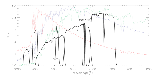
Figure 1: Spectra of typical F- (red) G- (blue) K- (green) type stars from MILES overplotted with the SAGES filter passbands.

The advantage of the SAGES filter system: which are more sensitive to stellar parameters than that of the traditional SC filter system. We utilized the Kurucz model (Munari et al., 2005) to analyze the dependence of the the colors of SAGES and the stellar parameters. We focus on the analysis of the gravity values log $g=2$ and 4.5, and the metallicity range of $\rm[Fe/H]=-2.5$ to 0.5. Figure 2 shows the effective temperature versus colors for different metallicities with two given gravity log $g=2.0$ (a) and 4.5 (b). It shows that the SAGES system is clearly much more sensitive to the effective temperature than that of the SC system. We can see that for the same effective temperature range, no matter which type of stars (FGK), the color range of SAGES is $\sim 2-3$ times of that in the SC system. In this case, the uncertainty of the effective temperature $T_{\rm eff}$ is 1/3 to 1/2 times of that in the SC system, improving the accuracy by $\sim 2-3$ times, i.e., the uncertainty of the effective temperature $T_{\rm eff}$ of a star of $V=15$ mag in the SC system is comparable to uncertainty $V\sim 16-16.5$ mag for the same star in the SAGES system (Fan et al., 2018).

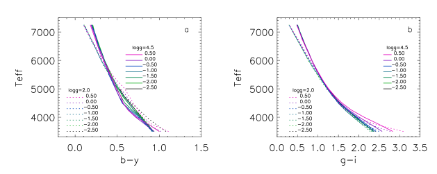
Figure 2: The effective temperature versus colors for different metallicities with two given gravities of log $g=2.0$ (a) and 4.5 (b).

Further, we have also investigated the relationship between the metallicity and colors of SC system (left panel) and SAGES (right panel). Figure 3 shows the relations between metallicity and colors of the SAGES for different effective temperatures with a given gravity of log $g=2.0$ and 4.5. Clearly, the SAGES system has higher sensitivity of the metallicity than that of the SC system. We can see that for the same metallicity range, no matter which type of stars (FGK), the color range of SAGES is $\sim 2-4$ times that of the SC system. In this case, the uncertainty of the metallicity $\rm[Fe/H]$ is 1/4 to 1/2 times of that in the SC system, improving the accuracy by $\sim 2-4$ times, i.e., the uncertainty of the metallicity $\rm[Fe/H]$ for a star of $V=15$ mag in the SC system is comparable to that of $v_{s}\sim 16-17$ mag for the same star in the SAGES system, which can be seen from the spectra of FGK stars shown in Figure 1.

Figure 3: Metallicity versus colors of the SC system (left panel) and SAGES (right panel) for different effective temperatures with a given gravity log $g=2.0$ and 4.5.

Figure 4 presents the relations between the gravity and colors of the SC system and SAGES for different effective temperatures. We consider two cases where the metallicity varies widely, e.g., for the metallicity $\rm[Fe/H]=-2.5$ and 0. For FG-type stars, the SAGE system is slightly more sensitive than the SC system (as shown in Figure 4). For K-type stars, the SC system has a serious ”S - shape” i.e., the non-monotonic relation. Although the SAGES system also shows a non-monotonic condition, the relationship between gravity and color is a monotonic function in the interval between log $g\gtrsim 2$ and log $g\lesssim 2$ if the distinction is made at log $g\approx 2$. We use the DDO51 filter, which can effectively distinguish dwarf stars and giant stars, to provide a feasible solution of gravity log $g$ for K-type stars, which is clearly the advantage of the SAGES photometric system (Fan et al., 2018).

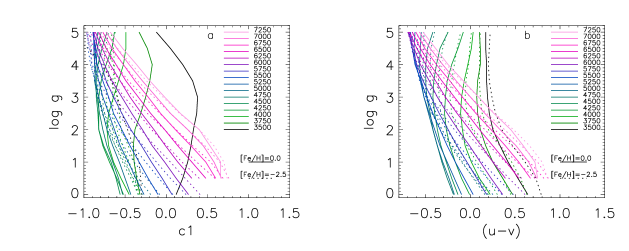
Figure 4: Gravity versus colors of the SC system (left panel) and SAGES (right panel) for different effective temperatures with solar metallicity.

Figure 5 shows the relation between the effective temperature $T_{\rm eff}$ and colors of SAGES for different gravity log $g$ with solar metallicity, where log $g=4.5$ for the panels of a, b, c and d; log $g=2.0$ for for the panels of e, f, g and h. For comparison, a, c, e and g panels are for the SC system and b, d, f and e panels are for SAGES. For G- and K-type stars, the absorption line strength of H$\beta$ is weaker than that of H$\alpha$, proving the intensity measurement accuracy of H$\alpha$ is higher. The relationship between the color index and different extinctions can be obtained by calculation. We take log $g=2$ and 4.5 and $\rm[Fe/H]=0$. Figure 5 shows the extinction variations in the relations between effective temperature and color: $g-I$ is more sensitive to effective temperature than $b-y$; For different extinction, $\beta_{n}-\beta_{w}$ has a certain color change ($\sim 0.01$ mag), while for $\alpha_{n}-\alpha_{w}$, the change with extinction is almost invisible (E(B$-$V) ranges from 0 to 0.2), suggesting that the latter is more independent of interstellar extinction. Thus the solution will be more accurate (Fan et al., 2018) for $\alpha_{n}-\alpha_{w}$ than that for $\beta_{n}-\beta_{w}$.

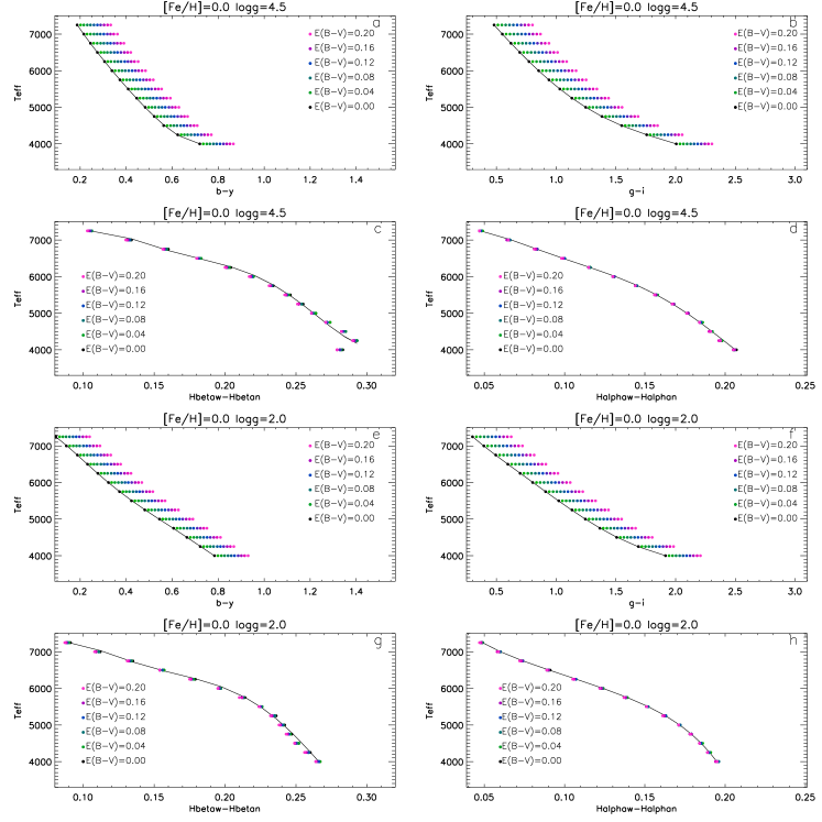
Figure 5: The extinction variations in the effective temperature $T_{\rm eff}$ versus colors of the SAGES for different log $g$ with solar metallicity and comparisons of the $\beta_{n}-\beta_{w}$ and $\alpha_{n}-\alpha_{w}$ for the extinction variations. The gravity log $g=4.5$ for the panels of a, b, c and d, while log $g=2.0$ for the panels of e, f, g and h; a, c, e and g panels are for the SC system and b, d, f and e panels are for the SAGES.

2.3 Telescopes and Detectors of SAGES

For the $u_{s}$- and $v_{s}$-passband observations were carried out with the 90-inch (2.3-m) Bok telescope in Kitt Peak of Arizona, USA. The prime focus is adopted for the survey, with corrected focal ratio of f/2.98 and corrected focal length of 6829.2 mm. The altitude of Kitt Peak National Observatory (KPNO, 111^∘36’01”.6W, +30^∘57’46”.5N) is 2071 meter. The location offers very stable seeing conditions and a fairly low horizon in all directions save for the northeast. The sky brightness measurements of Kitt Peak in 2009 are 22.79 mag arcsec^-2 in B and between 21.95 mag arcsec^-2 in V band (Neugent & Massey, 2010). For the location of the Bok telescope, the typical seeing was $1^{\prime\prime}.5$ during the observations. For the Bok telescope, an 8K $\times$ 8K CCD mosaic is composed of four 4K $\times$ 4K blue optimized sensitive back luminous CCDs, with gaps along both the RA (166^′′) and Dec directions (54^′′), by the University of Arizona Imaging Technology Laboratory (ITL). In figure 6, we can see the distribution of the four CCD arrays at the prime focus of the Bok telescope. The QE is $\sim$80 % for the u-band (central wavelength of $\sim 3538$ Å with FWHM of 520 Å) and the edge-to-edge field of view (FOV) is about $1^{\circ}.08\times 1^{\circ}.03$ (Zou et al., 2015, 2016; Zhou et al., 2016). In this paper, only the observing data of 2.3-m Bok telescope are released.

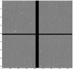
Figure 6: The image of the Bok telesocpe in the SAGES $v_{s}$ band. The CCD mosaic is composed of four CCDs and for each one there are four amplifiers.

The observing data of the following three telescopes are not included in this paper and will be released in following works:

For the $gri$ passband, NOWT of Xinjiang Observatory, CAS; A one-meter wide field astronomical telescope with Alt-Az mount, operating at prime focus with a field corrector. The NOWT provides excellent optical quality, pointing accuracy and tracking accuracy. It is located at Nanshan (87^∘10.67^′E, 43^∘28.27^′ N) with an altitude of 2080 m, which is $\sim$75 km away from Urumqi city. A 4K $\times$ 4K CCD was mounted on the prime focus of the telescope. The FOV at prime focus is $1.5^{\circ}\times 1.5^{\circ}$, and pointing accuracy is better than $5^{\prime\prime}$ RMS for each axis after pointing model correction (Liu et al., 2013).

For the $\alpha_{n}$ passband and part of $\alpha_{w}$ passband, 1-m Zeiss telescope of Maidanak astronomical observatory (MAO, 66^∘53’47”E, 38^∘40’ 22”N), which belongs to Ulugh Beg Astronomical Institute (UBAI), Uzbekistan. UBAI is an observational facility of the Uzbekistan Academy of Sciences (UAS). The total amount of clear night time is 2000 hours with median seeing of 0^′′.70. The altitude is 2593 meter. Based on two month observation performed in 1976, it shows that the sky background of Mount Maidanak varies between $22.3-22.9$ mag arcsec^-2 in B and between $21.4-22.0$ mag arcsec^-2 in V band (Kardopolov & Filip’ev, 1976). Its current field of view is $32.9^{\prime}\times 32.9^{\prime}$. For the narrow-band photometry, if the focal ratio is too fast, the central wavelength and the bandwidth will shift to some extent. For its Cassegrain focus, the focal ratio is f/13. However, in order to enlarge the FOV, we installed a focal reducer to make the focal ratio f/6.5, which is still suitable for the narrow-band survey. A 2K $\times$ 2K Andor DZ936 CCD was mounted on the f/6.5 Cassegrain focus of the telescope, to ensure that there is no wavelength shift or bandwidth changes for the narrow-band filters (Ehgamberdiev, 2000, 2018).

For the $\alpha_{w}$ and DDO51 band, Xuyi 1-m Schmidt telescope of Purple Mountain Observatory (PMO) of CAS: The Xuyi Schmidt Telescope is a traditional ground-based refractive-reflective telescope with a diameter of 1.04/1.20 meter. It is equipped with a 10K $\times$ 10K thinned CCD camera, yielding a $3.02^{\circ}\times 3.02^{\circ}$ effective FOV at a sampling of $1^{\prime\prime}.03$ per pixel projected on the sky. The QE of the CCD, at the cooled working temperature of $-103.45^{\circ}$ C, has a peak value of 90% in the blue and remains above 70% even to wavelengths as long as 8000 Å . The XSTPS-GAC was carried out with the SDSS $g$, $r$ and $i$ filters. The current work presents measurements of the Xuyi atmospheric extinction coefficients and the night sky brightness in the three SDSS filters based on the images collected by the XSTPS-GAC. The night sky brightness determined from images with good quality has median values of 21.7, 20.8 and 20.0 mag arcsec^-2 and reaches 22.1, 21.2 and 20.4 mag arcsec^-2 under the best observing conditions for the $g$, $r$ and $i$ bands, respectively (Zhang et al., 2013). The typical limiting magnitude is of $m(r)\sim 20.0$ mag.

2.4 Observing Strategy and Coverage

Figure 7 shows the survey area (in grey) in equatorial coordinates. The SAGES covers most of the northern sky area except the Galactic plane, for which the Galactic latitude $|b|>10$ degree and the declination is from $-5^{\circ}$ to $+90^{\circ}$. The total planned survey area $>12,000$ degree², which is $\sim 60\%$ of the northern hemisphere.

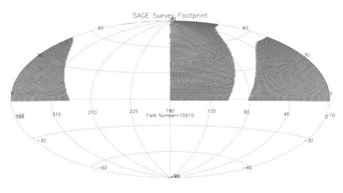
Figure 7: The sky coverage of the SAGES project covers most of the northern sky area except the Galactic plane, for which the Galactic latitude $|b|>10$ degree and the declination is from $-5^{\circ}$ to $+90^{\circ}$. The total survey area is $\sim$12,000 degree².

On the top panel, Figure 8 presents the sky coverage for SAGES in $u_{s}$/$v_{s}$ observations carried out with the Bok 2.3-m telescope. It covers the sky area of $\sim 9960$ degree², which is actually $\sim 87.8\%$ of the fields in total observed for SAGES in both passbands. Finally we obtained 23,980 frames for $u_{s}$-band and 17,565 frames for $v_{s}$ band. Among these images, 36,092 frames have better quality while the rest frames, which have been excluded, are defined in the following:

1. The frames with failed astrometry in data processing have been removed;

2. For the early testing frames of exposure very short, like 3 seconds 6 seconds, were removed;

3. No LAMOST standard stars and the number of common sources with the surrounding celestial region is very small, which also have been removed.

These ”better quality” frames are involved the flux calibration, which have been released in this paper.

The bottom panel shows that the the $gri$ passbands of SAGES. So far we have finished the observations for the designed area with the NOWT, which can be combined with the SDSS data for the brighter part of the catalog. The $gri$-band data of NOWT will be released in following papers.

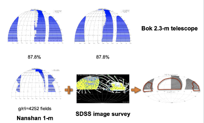
Figure 8: The sky coverage for the SAGES in $u_{s}$/$v_{s}$ passband is shown on the top panel. About $87.8\%$ of the fields in total have been observed for SAGES in both passbands, which uses the Bok 2.3m telescope. For the $gri$ passbands (which are shown on the bottom panel), we have finished the observations for the designed area with the NOWT, which can be combined with the SDSS data for the brighter part of the catalog. The $gri$-band data of NOWT will be released in following papers.

Figure 9 shows the airmass distribution for SAGES observations, with the median value of 1.11, and extending to airmass of 1.5 as the airmass limit of our observations was set to 1.5 in the observing strategy. Clearly for most of the fields, the airmass is less than 1.2, which can ensure that our images maintain good quality. This aspect has been incorporated in our survey strategy.

Figure 9: The airmass distribution for SAGES observations, with the median value of 1.10. Clearly for most of the fields, the airmass is less than 1.2, which can ensure the quality of our images. This aspect has been incorporated in our survey strategy.

For the $gri$ passbands, we have completed the observations for the designed area with the NOWT of XAO, which can be combined with the SDSS data. NOWT $gri$+SDSS survey imaging coverage is the total area for the initial plan of SAGES. The $gri$ band data of NOWT are not included in this paper and will be released in following papers. However, after the Pan-STARRS DR1 (PS1) data were released, since the sky coverage is large and the observing is homogeneous, it is a better choice for us to use the PS1 data of gri band instead of the NOWT $gri$ +SDSS survey data for the current work. Another reason is the PS1 can match our SAGES better in the magnitude range. However, in the future work, the NOWT $gri$ data also can be used for the stellar parameter estimates.

3 Data Pipeline

3.1 Image Processing

The raw data of SAGES are processed with the pipeline developed by our data reduction team. The basic corrections of overscan, bias, flat, and crosstalk effect are the same as the data reduction pipelines for most similar surveys.

For the bias correction, we took a set of 10 bias frames before and after the sky survey observations respectively every observing night. We constructed the combined master bias frame every night by using the median value of the 20 exposures at the same pixel. Thus both the science images and the flat-field images will be corrected for bias by applying this master bias image, which are not only corrected for the mean value of bias but also for the structure of bias (Zheng et al., 2018, 2019).

For the flat-fielding, we took the dome flats with a screen and a UV lamp to correct the pixel-to-pixel variations. Also we took the twilight flats to correct large-scale illumination trend if possible. Otherwise, a super night-sky flat will be used instead, which is the combination of all the science images taken over the night. For most nights, the uncertainty of the master flat images was less than 1%.

For the highly efficient readout mode can significantly reduce the time spent on reading the detector. However, it induces amplifier cross-talk, which may cause contamination across the output amplifiers at the symmetric place, typically at the level of 1:10,000 of the flux. This effect usually is quite significant for bright saturated stars on the CCD chips. A large number of images have been used to estimate the crosstalk coefficients between amplifiers. The overall ratio of crosstalk is at the level of 5:10,000 for 90Prime, while the inter-CCD crosstalk ratios are greater and intra-CCD ratios are lower.

Figure 6 is one image in the SAGES $v_{s}$-band of the survey. The CCD mosaic is composed of four $\rm 4K\times 4K$ blue sensitive back-luminated CCDs. For each CCD, the four-amplifier readout mode is applied, which has a faster readout speed.

3.2 Photometry

As mentioned above in the Section 2.4, we obtained 23,980 frames for the $u_{s}$-band and 17,565 frames for the $v_{s}$ band. In total we have 41,545 frames for $u_{s}$ and $v_{s}$ bands. Among these images, we have 36,092 frames with better quality and which involve flux calibration.

In our SAGES pipeline for photometry, we applied the Source Extractor (SE, Bertin & Armouts, 1996) for detecting sources and photometry. The detection threshold is set to 4 (sigma above the background rms), which can make sure that most sources could be detected and measured precisely. SE could provide the following measurements and errors: the central positions of each source in both CCD physical coordinates and celestial coordinates, the roundness and sharpness, and instrumental magnitudes are included in a series of given apertures.

As we know, for the different photometric methods, the routine will produce different results. We use the software SE MAG_AUTO as our primary output parameters, as this output is in general reasonable for both point sources and extended sources. In our photometric pipeline, the aperture correction needs to be applied to aperture photometry, which is using the aperture growth-curve method.

In the SAGES photometric calibration, we adopted the “AB system” (Oke & Gunn, 1983) which is more commonly used for the photometric system, as it is well-known for the Sloan Digital Sky Survey (SDSS) (York et al., 2000) by Fukugita et al. (1996). For our calibration, the comparisons show that the SAGES implementation of the AB system has an accuracy of $\sim$0.02 mag (90% confidence). The dominant contribution is the uncertainty in how well spectrophotometry matches the AB system.

Figure 10 shows the flow chart of the photometry pipeline for SAGES, which uses SE as the main routine for photometry. The bias and overscan are combined for the correction. We use the super-flats as final flat for the correction, which is more reasonable for our data reduction.

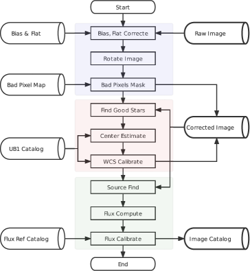
Figure 10: The flow chart of photometric pipeline for SAGES data reduction.

Figure 11 is the plot of the photometry uncertainties versus the magnitude of SAGES in the $u_{s}$-band and the $v_{s}$-band. Here the photometry uncertainties are just from the poisson statistics, which are not the rms of repeat observations, since for most sources we just observed for only one time. It can be seen that the limiting magnitude is $\sim 17$ mag for both the $u_{s}$-band and the $v_{s}$-band of SAGES, for the uncertainties of the magnitude of 0.01 mag, which correspond to the S/N$\sim 100$ and different from the complete magnitude.

Figure 11: The photometry uncertainties (from poisson statistics) vs. magnitude in the SAGES project in the $u_{s}$-band (top) and $v_{s}$-band (bottom) for a typical field. The limiting magnitude is $\sim 17$ mag for both the $u_{s}$-band and the $v_{s}$-band of SAGES, with uncertainties of 0.01 mag, which corresponds to S/N$\sim 100$.

3.3 Astrometry

The astrometric calibration is realized in two steps. Firstly, the pipeline will work out a linear solution assuming the image has no distortion, based on the information stored in image headers, including the telescope pointing coordinates, the rotation angle, and the pixel scale. For further corrections, the pipeline employs the package named SCAMP (Software for Calibrating AstroMetry and Photometry, https://www.astromatic.net/software/scamp/), which is a computer program that computes astrometric projection parameters. Otherwise, SCAMP is mature and robust software that is widely used in astrometric calibration by matching SExtractor’s output catalog with an online or local reference catalog (Bertin & Armouts, 1996).

Our pipeline runs SCAMP twice: for the first run, we use a loose criterion for cross-matching detected sources with reference sources, which is in order to maintain enough stars in the image for calibration; for the second run, we applied a more strict criterion to obtain a more precise solution based on the previous results. Table 2 shows the configuration parameters for SCAMP in our pipeline for the two runs. It is found that DISTORT DEGREES $=3$ is the most proper configuration after a series of tests (Zheng et al., 2018, 2019).

In our astrometric pipeline, we use the Position and Proper Motion Extended (PPMX) (Roser et al., 2008) as the astrometric reference, which contains $\sim$18 million stars. The reference stars are distributed across the whole sky with the astrometric accuracy of $\sim 0^{\prime\prime}.02$ in both R.A. and Dec (Zheng et al., 2018, 2019).

Although Pan-STARRS DR1 (PS1) (Chambers et al., 2016) has an accurate position estimate, i.e., both uncertainties are lower than $0^{\prime\prime}$.005 in both R.A. and Dec directions, PS1 does not have information on proper motions. Thus we do not use the PS1 catalog as the astrometric reference, and we use it as the flux reference (see Section 3.4). We use PPMX as the astrometric reference. In fact, in the matching with our SAGES, $>85$% of the PPMX stars are in the magnitude range of 10.0$<$ V$<$ 15.0 mag. As the Gaia DR3 has been released, we may improve the precision of the astrometric reference in future work. Due to the lack of providing the astrometric residuals, we cannot check the solution is correct or not. In addition, besides SCAMP, we also developed another astrometric calibration method SIP (Simple Imaging Polynomial) (Shupe et al., 2005) for providing an astrometric solution, since SCAMP does not provide the fitting errors which can be used to judge the results are good enough or not. Therefore, in the astrometric pipeline, we applied both methods to make sure the solution is correct and accurate.

In our astrometric pipeline, we first convert the original pixel coordinates (x, y) with origin at the left-bottom corner of one single frame (one chip), to intermediate pixel coordinates ($u_{s}$, $v_{s}$) with the origin at the center of the whole FOV. The second step is to convert the ($u_{s}$, $v_{s}$) to the intermediate world coordinates ($\epsilon$, $\eta$) with parameters CD_ij recorded in the fits header. The parameters CD present a matrix which transfers from (u, v) to ($\epsilon$, $\eta$). Initially, they can be computed by the rotate angle and the pixel-scale of detector. They are provided in headers after the header fixing process. Finally, the intermediate world coordinates ($\epsilon$, $\eta$) are projected to the world coordinates ($\alpha$, $\delta$), with the projection type of “TAN”. In order to resolve the non-linear correlation transformation between ($\epsilon$, $\eta$) and ($\alpha$, $\delta$), we applied the SIP convention to represent image distortion as it introduces high-order correction polynomials f and g to $u_{s}$, $v_{s}$ to express the distortion, as in formula 1 (Zheng et al., 2018, 2019).

$$\left(\begin{array}[]{c}\epsilon\\ \eta\\ \end{array}\right)=CD\times\left(\begin{array}[]{c}u+f(u,v)\\ v+g(u,v)\\ \end{array}\right)$$

In our transform of the astrometry, $A_{pq}$ and $B_{pq}$ are used as the coefficients of $u^{p}v^{q}$ as shown in Formula 2 to determine polynomials f and g, in which $N_{A}$ and $N_{B}$ are the highest order to correct $u_{s}$ and $v_{s}$. We adopt appropriate parameters NA $=$ NB $=3$ for the SAGES.

$$f(u,v)=\sum_{p,q}A_{pq}\cdot u^{p}v^{q},2\leq p+q\leq N_{A}$$

$$g(u,v)=\sum_{p,q}B_{pq}\cdot u^{p}v^{q},2\leq p+q\leq N_{B}$$

We use the multiple visits, no matter if in the same band or not, to estimate the differences in coordinates between different visits. Figure 12 shows a typical internal astrometric error of one image, in which it shows that $\Delta R.A.=0^{\prime\prime}.014\pm 0^{\prime\prime}.145$ and $\Delta Dec=-0^{\prime\prime}.002\pm 0^{\prime\prime}.166$. The external astrometric errors are estimated by comparing the difference between the coordinates from our catalog and those from reference catalog PPMX. Figure 10 shows a typical distribution of external astrometric calibration errors in one observing field. It can be seen that the standard deviations is quite small, i.e., $\sim 0^{\prime\prime}.1$ in both R.A. and Dec directions, as marked in the lower-left panel, which includes both internal and external astrometric uncertainties in both directions (Zheng et al., 2018, 2019). In the future work, it can be improved when employing Gaia DR3 as a reference catalog.

Figure 12: The precision of the astrometry in the SAGES project in the $u_{s}$-band (top) and $v_{s}$-band (bottom) for one typical image. The external astrometric errors are estimated by comparing the difference between the coordinates from our catalog and those from reference catalog PPMX.

Figure 13 is the flow chart of the SIP for the SAGES astrometry, which adopt the Source Extractor results as the input catalog and applies the fits header as the WCS initial value. The task SCAMP is applied twice and we use the PPMX as the reference catalog.

Figure 13: The flow chart of the SIP for SAGES astrometry after two runs of the SCAMP. In our work, we applied the pipeline based on the SCAMP and our routine SIP.

Table 2 shows the configuration parameter of astrometry table for SCAMP, which has been applied for our data reduction pipeline.

Table 2: The configuration parameter of astrometry table for SCAMP applied in our pipeline.

Keywords	Round 1	Round 2	Notes
MATCH	Y	Y	Module match or not
MATCH_NMAX	0	0	up bound of cross match
PIXSCALE_MAXERR	2	1.5	Max error of pixel scale
POSANGLE_MAXERR	5.0	2.0	Max error of position angle (degree)
POSITION_MAXERR	10.0	1.0	Max error position
MATCH_RESOL	0	0	matching resolving
MATCH_FLIPPED	N	N	Allow axis flipping in match or not
CROSSID_RADIUS	25.0	25.0	Cross identification radius
SOLVE_ASTROM	Y	Y	Solve astrometric solution or not
PROJECTION_TYPE	SAME	SAME	Projection type
DISTORT_DEGREES	3	3	Degree of Distortion Polynomial

3.4 Flux Calibration

In this work, using the spectroscopic data from the Large Sky Area Multi-Object Fiber Spectroscopic Telescope (LAMOST; Cui et al. 2012; Zhao et al. 2012) DR5, photometric data from the Gaia DR2 (Gaia Collaboration et al. 2016, 2018), and over-lapping observations of the SAGES, we first perform the relative flux calibration of SAGES DR1 $u_{s}$/$v_{s}$ bands by combining the Stellar Color Regression (SCR; Yuan et al. 2015) method and the Ubercalibration method (Padmanabhan et al., 2008). The absolute calibration is then carried out by comparing with synthetic colors from the MILES library (http://research.iac.es/proyecto/miles/) (Sanchez-Blazquez et al., 2006).

In fact, Yuan et al. (2015) have proposed the spectroscopy-based SCR method to perform precise color calibrations by using millions of spectroscopically observed stars as color standards, with the star-pair technique (Yuan et al., 2013), which considers that stellar colors can be accurately predicted by large-scale spectroscopic surveys, e.g., SDSS, LAMOST.

Combining with the accurate and homogeneous photometric data from Gaia DR2 and Early Data Release 3 (EDR3; Gaia Collaboration et al. 2021a, b), the method can further accurately predict the magnitudes of stars in various passbands and perform high precision photometric calibration. Such method has been applied to a number of surveys, including the SDSS Stripe 82 (Yuan et al., 2015; Huang et al., 2022), the SkyMapper Southern Survey DR2 (Huang et al., 2021), the Gaia DR2 and EDR3 (Niu et al. 2021a, b), and the PS1 DR1 (Xiao & Yuan, 2022). A precision of 1 to a few mmag is usually achieved. A recent review of the method and its implementations can be found in Huang et al. (2022).

The Ubercalibration method was originally developed for SDSS, and achieved a precision of 1% in the griz bands, and 2% in the $u$ band (Padmanabhan et al., 2008). It requires a significant amount of over-lapping/repeating observations and assumes that the physical magnitude of the same object under different observational conditions should be the same. Schlafly et al. (2012) have applied the method to PS1 catalogs, achieving a precision of better than 1%. The method has also been applied to the Beijing–Arizona Sky Survey (BASS) (Zou et al., 2017; Zhou et al., 2018), achieving a precision of better than 1%. A detailed summary and discussion of limitations of the method can be found in Huang et al. (2022).

We combine the two aforementioned methods to perform the relative flux calibration of SAGES DR1 $u_{s}$/$v_{s}$ bands. A detailed description of the calibration process will be presented in a separate paper (Yuan H. et al. in preparation). Here we briefly outline the calibration strategy.

The calibration process of SAGES DR1 is carried out for each gate separately in the $u_{s}$ and $v_{s}$ bands. We assume that the relative calibrated magnitude of an object $m_{\rm rel}$ can be derived from its instrumental magnitude $m$ by

$$m_{\rm rel}=m+zp\_frame(i)+zp\_gate\_corr(i,j)+flat\_corr(day,j,X,Y),$$ (1)

where $zp\_frame(i)$ is the zero point of the $i$-th frame, $zp\_gate\_corr(i,j)$ is the zero point correction of the $j$-th gate of the $i$-th frame, and $flat\_corr(day,j,X,Y)$ is the daily star flat correction of the $j$-th gate and depends on CCD position (X, Y). Taking u_s band for example, the detailed calibration strategy is listed as below:

1. Combine the SAGES DR1 photometric data with LAMOST DR5 and the Gaia DR2 to create a sample for the flux-calibration, which have data from all the three database above. Select dwarfs as the calibration stars with the following constraints: (1) $5300<T_{\rm eff}<6800$ K and $-0.8<\rm[Fe/H]<0.2$, a narrow temperature and metallicity range for robust fitting of stellar colors as a function of stellar atmospheric parameters; and (2) Signal-to-noise ratio ($\rm S/N_{g}$) of the LAMOST spectra $>20$. About 1.5 and 1.1 million calibration stars are selected for the $u_{s}$ and $v_{s}$ bands, respectively.

2. Fit stellar intrinsic color – stellar atmospheric parameters relation $(G_{\rm BP}-u_{s})_{0}$ = $f(T_{\rm eff},\rm[Fe/H])$ using stars from two-well selected neighboring fields which have more LAMOST targets for calibration. Here $f(T_{\rm eff},\rm[Fe/H])$ is a second-order two-dimensional polynomial with six free parameters. The neighboring fields means that they have similar position and observing time, thus they should have similar zero-points so that they can be regarded as one field and have more sources.

   $$f(T_{\rm eff},\rm[Fe/H])= {a_{0}}\cdot T_{\rm eff}^{2}+{a_{1}}\cdot{\rm[Fe/H]}^{2}+{a_{2}}\cdot T_{\rm eff}\cdot{\rm[Fe/H]}+{a_{3}}\cdot T_{\rm eff}+{a_{4}}\cdot{\rm[Fe/H]}+{a_{5}}.$$ (2)

3. Estimate the predicted magnitudes for all the calibration stars with a typical precision of $2-3\%$, and obtain zero point of each gate of each image file.

4. Construct the daily star flat for each gate $flat\_corr(day,j,X,Y)$ using second-order two-dimensional polynomials as a function of $X$ and $Y$.

5. After star flat correction, obtain zero point of each image file $zp\_frame(i)$ and zero point correction $zp\_gate\_corr(i,j)$ of each gate and each image file.

6. Go to step b, reconstruct the relation, and iterate.

7. Combine the ubercalibration method and the SCR method to further improve the calibration, particularly for the image files with nil or a small number of LAMOST standard stars.

8. At last, perform absolute calibration by comparing the color-color relationship ($G_{\rm BP}-u_{s}~{}vs.~{}G_{\rm BP}-G_{\rm RP}$) between the observed and synthesized cases from the empirical MILES spectral library.

Reddening correction in steps b and c is performed using $E(BP-RP)$ and empirical temperature- and reddening- dependent reddening coefficients, both of which are obtained using the star-pair technique similar to the one in Sun et al. (2022). Applying the above procedure, we have achieved an internal calibration precision of around 5 mmag for the SAGES DR1 data by comparing repeated observations.

Figure 14 shows the color-magnitude and color-color diagrams of M67 with the SAGES and Gaia DR2 photometry but the DR3 will not change much. It can be seen that our SAGES photometric precision is comparable to that of the Gaia BP/RP. The red dots are the giants and black dots are the dwarfs. We can see that the giants and dwarfs can be separated very well.

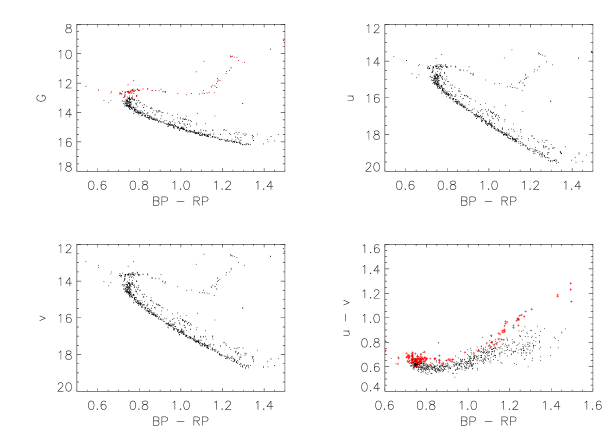
Figure 14: The color-magnitude of the M67 cluster with SAGES and Gaia DR2 photometry. The red dots are the giants and the black dots are the dwarfs. The giants and dwarfs can be well separated in the color-color diagram (bottom right).

3.5 Cross-Matched External Catalogs

As in SAGES DR1, we mainly cross-match the master table with PS1 catalogs as its observing depth is comparable to our $u_{s}$ and $v_{s}$ passband. Although we have the complete $gri$-passband observations of the 1-m telescope at the Nanshan station of XAO, it is not deep enough. Previously we planned to combine our observations of XAO to complement the SDSS imaging survey. However, it is well known that the combination of the two kinds of survey data may not be homogeneous for the observations depth. Also we need the transformations of the passband between the Nanshan data and the SDSS data.

Thus we combined our $u_{s}$ and $v_{s}$ band data with the PS1, which is homogeneous and sky coverage is large enough, i.e, $\sim 3/4$ of the total sky. For large photometric catalogs, we determine the matching external object and record its ID and projected distance within the master table. In our work, we match in the reverse direction and distance in the external catalog as DR1-ID. However, the proper motion information is not included in the catalog. The maximum distance for all cross-matches is $2^{\prime\prime}$, motivated by the region in which our 1D PSF magnitudes may be affected.

Such matching process has resulted in a catalog with half of the original sources. There are 39,857,439 sources and 42,457,643 sources left in the $u_{s}$ and $v_{s}$ passbands respectively after combining with the PS1 catalog.

4 Data Products of SAGES

4.1 The Contents of SAGES DR1

The SAGES Data Release 1 contains the total photometry from a total of 36,092 image exposures, including 23,980 images in $u_{s}$ passband and 17,565 images in the $v_{s}$ passband. In total we have 41,545 frames for $u_{s}$ and $v_{s}$ bands. Among these images, 36,092 frames have high quality and involve the flux calibration. After combining with the PS1 catalog, the SAGES Master catalog thus contains a total number of 54,215,563 sources which will be actually released in this paper.

4.1.1 The SAGES Master Table

The SAGES DR1 total photometric table contains about one hundred million unique astrophysical objects in either SAGES $u_{s}$ and $v_{s}$ bands. The astrometric calibration of DR1 is accomplished and the median offset between our positions and those in Gaia DR2 is 0^′′.16 for all objects and 0^′′.12 for bright, well-measured objects. In the next release, we plan to switch the astrometric reference frame to Gaia DR3.

Table 3 shows the header of the SAGES master catalog, including the parameters of NUMBER, RA, RA$\_$ERR, DEC, DEC$\_$ERR, U$\_$COUNT, U$\_$MAG$\_$AUTO, U$\_$ERR$\_$ISOCOR, U$\_$ERR$\_$ISOCOR, etc. as well as the information of the PS1 catalog, such as the photometry, errors and IDs.

Table 3: The contents and descriptions of the SAGES Master catalog.

Parameters	Descriptions of SAGES Master Catalog
NUMBER	Running object number
RA	Right ascension of object (J2000)
$\rm RA\_ERR$	the Error of Right ascension
DEC	Declination of the object (J2000)
$\rm DEC\_ERR$	the Error of Declination
$\rm u\_FLUX$	data counts of $\rm AUTO\_FLUX$
$\rm u\_MAG\_AUTO$	AUTO magnitude in the $u_{S}$ passband
$\rm u\_ERR\_AUTO$	photometry error of AUTO magnitude
$\rm u\_MAG\_ISOCOR$	Isophotal magnitude in $u_{S}$-band
$\rm u\_ERR\_ISOCOR$	photometry error of Isophotal magnitude in $u_{S}$-band
$\rm u\_MAG\_APERCOR$	aperture magnitude in $u_{S}$-band
$\rm u\_ERR\_APERCOR$	photometry error of aperture magnitude in $u_{S}$-band
$\rm u\_MAG\_PETRO$	Petrosian-like elliptical aperture magnitude in $u_{S}$-band
$\rm u\_ERR\_PETRO$	photometry error of Petrosian-like elliptical aperture magnitude in $u_{S}$-band
$\rm u\_FLAGS$	Combination method for flags on the same object: 17 – arithmetical OR,
	18 – arithmetical AND, 19 – minimum of all flag values, 20 – maximum of all flag values,
	21 – most common flag value
$\rm v\_FLUX$	data counts of $\rm AUTO\_FLUX$
$\rm v\_MAG\_AUTO$	AUTO magnitude in the $v_{S}$ passband
$\rm v\_ERR\_AUTO$	photometry error of AUTO magnitude
$\rm v\_MAG\_ISOCOR$	Isophotal magnitude in $v_{S}$-band
$\rm v\_ERR\_ISOCOR$	photometry error of Isophotal magnitude in $v_{S}$-band
$\rm v\_MAG\_APERCOR$	aperture magnitude in $v_{S}$-band
$\rm v\_ERR\_APERCOR$	photometry error of aperture magnitude in $v_{S}$-band
$\rm v\_MAG\_PETRO$	Petrosian-like elliptical aperture magnitude in $v_{S}$-band
$\rm v\_ERR\_PETRO$	photometry error of Petrosian-like elliptical aperture magnitude in $v_{S}$-band
$\rm v\_FLAGS$	Combination method for flags on the same object: 17 – arithmetical OR,
	18 – arithmetical AND, 19 – minimum of all flag values, 20 – maximum of all flag values,
	21 – most common flag value
$\rm g\_MAG\_PS1$	g mag of Pan-STARRS
$\rm g\_ERR\_PS1$	photometry error of g mag of Pan-STARRS catalog
$\rm r\_MAG\_PS1$	r mag of Pan-STARRS
$\rm r\_MAG\_PS1$	photometry error of r mag of Pan-STARRS catalog
$\rm i\_MAG\_PS1$	i mag of Pan-STARRS
$\rm i\_ERR\_PS1$	photometry error of i mag of Pan-STARRS catalog
$\rm ID\_PS1$	ID from Pan-STARRS catalog

The photometric measurement can be qualified through the SE FLAGS (reliable 0 to 3, and caution should be taken for $>4$) .

Table 4: The contents and descriptions of the SAGES merge Bits table.

Bits	Represents Meaning
0	Detected only once
1	Has other close objects but rejected while merging
2	Flux not good enough, at least 1 source is out of 3$\sigma$
3	Position not good enough, at least 1 source is out of 3$\sigma$
4-27	Reserved
28	No matched object
29-31	Reserved

4.1.2 Limitation of auto- and aperture magnitudes

Figure 15 shows the magnitude distribution of the SAGES $u_{s}$ and $v_{s}$ bands for all the sources of the SAGES DR1 catalog in all our observing fields, including the sources fainter than the ”limiting magnitude”. We can see that for the $u_{s}$-band the limiting magnitude is around 20 mag while for the $v_{s}$-band, the limiting magnitude is around 21 mag.

Figure 15: The magnitude distribution of the SAGES $u_{s}$ and $v_{s}$ bands for all the sources of the SAGES catalog in all observed fields, even including the sources fainter than the ”limiting magnitude”. The y-axis represents the counts for the photometry magnitude number. It can be seen that the peaks are $u_{s}\sim 21$ mag and $v_{s}\sim 20.5$ mag for our SAGES photometry.

Figures 16-19 are the distributions of observing depth (i.e. limiting magnitude of different S/N and complete magnitude, (which defines as the turnover in the magnitude histogram)) of the SAGES survey for the best magnitude for the $u_{s}$-/$v_{s}$-passbands.

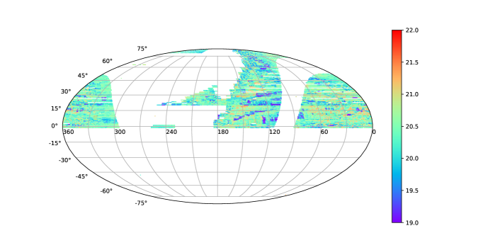
Figure 16: The observing area distribution of limiting magnitude in the SAGES $u_{s}$ passband for all fields for S/N=100, corresponding to the photometry error of 0.01 mag.

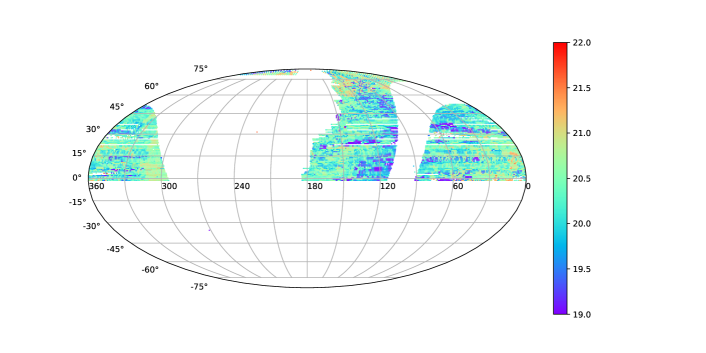
Figure 17: Similar to Figure 16 but for the SAGES $v_{s}$ passband, limiting magnitude for S/N=100, corresponding to the photometry error of 0.01 mag.

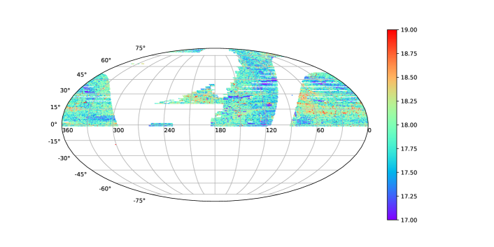
Figure 18: Similar to Figure 16 but for complete magnitude (which defines as the turnover in the magnitude histogram) of the SAGES $u_{s}$ passband, which is $\sim 2.4$ mag deeper than that in Figure 16.

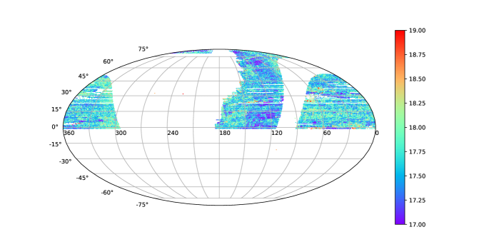
Figure 19: Similar to Figure 16 but for complete magnitude of the SAGES v_s passband, which is $\sim 2.4$ mag deeper than that in Figure 16.

Figures 20-21 are the distributions of the complete magnitude (which defines as the turnover in the magnitude histogram) in the SAGES $u_{s}$ and $v_{s}$ passband. The median values are $u_{s}\sim 20.4$ mag and $v_{s}\sim 20.3$ mag.

Figure 20: The distribution of the complete magnitude (which defines as the turnover in the magnitude histogram) of the SAGES $u_{s}$ passband for all fields, with the median value of $u_{s}=20.4$ mag.

Figure 21: Similar to Figure 20, but for the distribution of the complete magnitude in SAGES $v_{s}$ passband, with the median value of $v_{s}=20.3$ mag.

It is also possible that the photometry table does not reveal entries for an object in an image, which is clearly visible in the image in question. Unless SE overlooked the object, given the parameters we chose, this should only happen when SE extracted two objects in this image while they are considered children of a single parent object for this filter. If all images within one filter show multiple objects for what is taken to be a single merged object, all measurements for this object will be excluded from the photometry table and hence no distilled summary photometry for this filter shall be included in the master table.

4.2 Data Access of SAGES

Finally we have obtained a master catalog (Please see Table 5) for the SAGES DR1, which includes 93,293,120 items in $u_{s}$ band and 91,185,024 items in $v_{s}$ band. After combing with PS1, the numbers are reduced to 48,553,987 in our detection $u_{s}$ or $v_{s}$ band. The SAGES DR1 dataset will be available to the community through the China-VO platform and the National Astronomical Data Center (NADC) https://nadc.china-vo.org. The release can be browsed at the website, either in color or in each SAGES per passband.

The catalog structure includes the following:

1. The cross-matching to external catalogs now includes SAGES DR1 and PS1 DR1. Further, in the DR2 version, it will include the information of LAMOST and Gaia DR3, as well as 2MASS, AllWISE, GALEX, and UCAC4. The LAMOST catalog contains the stellar parameters of gravity, metallicity and temperature, while the Gaia DR3 contains the photometry of G-band, GB, GR band as well as the parallax and other information.

2. For the SAGES $u_{s}$ and $v_{s}$ passband, the photometry table also includes a column: if the sources have been measured 1, 2 or 4 times for the observations, as the overlapped with the adjacent fields. We only provide the combined magnitude in DR1. Thus for the exposure of 2 or 4 times, the photometry uncertainties are calculated as the variations of the magnitudes for different times. However, in the next version, the individual measurements of photometry may also be released.

Table 5: The item number for $u_{s}$ and $v_{s}$ passbands for combination themselves and combination with PS1.

Parameters	$u_{s}$-band	$v_{s}$-band
Total detection in $u_{s}$ or $v_{s}$	98,542,704
Before combination of $u_{s}$ or $v_{s}$	93,293,120	91,185,024
Combined with PS1	48,553,987

5 Examples of Science Cases

The sciences that can be done with a comprehensive survey such as the SAGES cannot be fully described or predicted. In the following, we outline a series of scientific goals that may have a high impact in addressing:

1. Metallicity distribution of the Milky Way halo

The observed metallicity distribution of the Galactic halo can not only help us understand its structure, as sub-structures in the halo often stand out in the space of metallicity, but also can provide the clue to processes involved in its formation history (Frebel & Norris, 2013). Especially, objects in the low-metallicity tail of the Milky Way metallicity distribution function (MDF) provide a unique observational window onto the time very shortly after the Big Bang. They provide key insights into the very beginning of Galactic chemical evolution (e.g., see Salvadori et al. 2010 for a typical example). Galactic MDFs obtained from the spectroscopic survey data usually suffer complicated selection function, whereas photometric survey projects provide a unique chance to solve the problem, e.g., recent experiments with the survey data from the SkyMapper survey (Youakim et al., 2020), the Pristine survey (Chiti et al., 2021), etc. With the large sky coverage and the metallicity sensitive-filter system, the SAGES data would be able to provide the best MDF of the Milky Way halo in the northern sky covering the very metal-poor tail, which furthermore results in the most complete halo MDF when combining with the southern data from SkyMapper, etc.

2. Searching for stars with the lowest metallicities

Stellar and supernova nucleosynthesis in the first few billion years of the cosmic history have set the scene for early structure formation in the Universe, while little is known about their nature (Bromm & Yoshida, 2011; Karlsson et al., 2013). Since it is not yet possible to directly observe processes of metal enrichment at high redshifts, the only observational probe of the metal enrichment sources in the early Universe has been chemical signatures retained in the atmosphere of nearby long-lived metal-poor stars in the Milky Way and nearby dwarf galaxies. Stars with the lowest iron abundances such as extremely metal-poor (EMP) stars with $[\rm{Fe/H}]<-3$ are commonly considered to be objects retaining chemical signatures of the Pop III nucleosynthesis (Beers & Christlieb, 2005; Frebel & Norris, 2015). With the robust metallicity estimated from the SAGES data, it would enable us to carry out the largest scale of searching project for EMP stars and stars with even lower metallicities in the northern sky, which would provide a valuable candidate database for medium-to-high-resolution follow-up observations. The resulting database of Galactic stars with the lowest metallicities can also be used as an important probe of early chemical evolution by comparing with chemical evolution models (e.g. Kobayashi et al., 2020).

4. Determine the shape and distribution of dark matter halo of the Milky Way

The Lambda Cold Dark Matter ($\Lambda$CDM) cosmological model predicts the existence of dark matter (DM) halos surrounding the Milky Way (MW) and external galaxies. Although to first order the spherically symmetric Navarro–Frenk–White (NFW) profile (Navarro et al., 1997) can provide a good approximation to the shape of the DM halos, the first numerical N-body simulations (Frenk et al., 1988; Dubinski & Carlberg, 1991; Warren et al., 1992; Cole & Lacey, 1996) found the shape of the DM halos to be triaxial, and subsequent works (e.g., Jing & Suto, 2002; Bailin & Steinmetz, 2005; Hayashi et al., 2007; Vera-Ciro et al., 2011) confirmed these results. With SAGES data, candidates blue horizontal branch (BHB) stars can be isolated by a machine learning approach through the application of ANN combined with color-color diagram. Since the absolute magnitude of a BHB star is relatively stable, the distance is easier to estimate. Then we can examine the number density of the inner halo with our BHB stars, which could constrain the shape of the halo.

5. Three-dimensional Distribution of Interstellar Dust in the Milky Way (north sky)

Extinction and reddening by interstellar dust grains pose a serious obstacle for the study of the structure and stellar populations of the Milky Way galaxy. In order to obtain the intrinsic luminosities or colors of the observed objects, one needs to correct for the dust extinction and reddening. Extinction maps are useful tools for this purpose. The traditional two-dimensional (2D) extinction maps, including those from dust emission in far-infrared (IR) (Schlegel et al., 1998, hereafter SFD), far-infrared combined with microwave (Planck Collaboration et al., 2014), and those derived from optical and near-IR stellar photometry (e.g., Schlafly et al., 2010; Majewski et al., 2011; Nidever et al., 2012; Gonzalez et al., 2012, 2018), give only the total or an average extinction for a given line of sight and therefore do not deliver information on the dust distribution as a function of distance. This can be particularly problematic for Galactic objects at a finite distance, especially those in the disk (Guo et al., 2021). The Rayleigh-Jeans Color Excess (RJCE) method of Majewski et al. (2011) gives the extinction on a star-by-star basis, so can be combined with the distance to individual stars in a similar fashion. The RJCE method is perhaps less accurate because it assumes that all stars have the same color in H-4.5 rather than getting the $T_{\rm eff}$ from these passbands, but that’s a different disadvantage. In Nidever et al. (2012) the RJCE results for individual stars are explicitly averaged for a 2-D map. With $\alpha_{w}-\alpha_{n}$ color, the relation of $T_{\rm eff}$ and $\alpha_{w}-\alpha_{n}$, the relation of $T_{\rm eff}$ and $g-i$, the e(g-i) can be estimated for each star, which is an independent method to obtain the extinction of all SAGES stars. Combined with the distance of each stars, we can construct the three-dimensional distribution of interstellar dust in the northern sky of the Milky Way, which will provide another more accurate dust map for the astronomical community.

6. Search and identifications for WD candidates

White dwarfs (WDs) are the final stage for the evolution of the majority of low- and medium-mass stars with initial masses $<8M_{\odot}$. The evolution of WDs is dominated by a well-understood cooling process (Fontaine et al., 2001; Salaris et al., 2000); because of no fusion reaction. WDs are powerful tools with applications in areas of astronomy, such as cosmochronology (see, Fontaine et al., 2001); constraints on the local star formation rate and history of the Galactic disk (Krzesinski et al., 2009); Initial-Final Mass Relation (IFMR) (Zhao et al., 2012); exoplanetary science (see, e.g., Hollands et al., 2018). With the spectroscopic survey (SDSS, Kleinman et al., 2013); (LAMOST, Zhao et al., 2013), etc. and photometric survey (such as Gaia, Gentile Fusillo et al., 2021), more and more WDs have been identified. SAGES is the new data source to search WDs candidates. By color-color diagram $g-i$ vs. $u-g$, the WDs can be selected with high confidence in SAGES (Li et al. in preparation). Then, the complete WDs sample with 100 pc will be constructed to set up the luminosity function, estimate the age of those sample etc. At the mean time, new filters (u,v) of SAGES can be used to fit SED, which provides more information for WDs population.

7. The substructures of the Milky Way

Large photometric surveys such as 2MASS, SDSS, and Pan-STARRS have revealed much tumult at the disc–halo interface through the discovery of numerous streams and cloud-like structures about the Galactic mid-plane out to large latitudes ($b<$40 degree) (Newberg et al., 2002; Slater et al., 2014). SAGES can provide more accurate stellar parameters. Thus, tracers such as RGB stars, BHB stars, etc are easier to separate. With different tracer samples, we try to search new streams with multiple methods, such as match-filter and integral of motion with the assumption of radial velocity distribution. We expect that several new streams in the relatively close inner halo can be detected with SAGES data. Also, for known substructures, we could identify their member candidates with SAGES data. Then their chemical properties will be obtained, which could provide constraints for their progenitors.

8. Other science cases, e.g., variable stars, QSOs

In recent years, time domain sciences have become more and more important. Although for the SAGES, we only obtain a single exposure for a certain field, we still can find the sources which have luminosity changes if combining with other observations in a similar passband, i.e., SDSS and SCUSS. A lot of observations suggest that active galactic nuclei (AGNs) and Quasi-Stellar Objects (QSOs) exhibit brightness changes in the optical bands. Rumbaugh et al. (2018) presented a sample of $\sim 1000$ extreme variability quasars (EVQs) with a maximum magnitude change in g-band over one mag with the observations of SDSS and Dark Energy Survey (DES) (Flaugher, 2005) imaging survey. Thus we can compare the $u_{s}$/$v_{s}$ band observations of SAGES with $u$-band observations of the SDSS and SCUSS to find the variable sources, i.e., the QSOs and the variable stars, through the magnitude and color transformations.

6 Future Plans and Data Releases

Since March 2015, observations of NOWT of XAO have focused on the $gri$ passband for the survey, data of which will be released in the further. Also the observations of the Xuyi 1-m telescope are still going on and we will release that part when the observations of DDO51 and H$\alpha$ passband have been finished.

The next data release of SAGES will contain more images and better sky coverage, as well as co-added sky tiles, where we homogenize the PSFs of images and then reregister and co-add them within filters. In the future, we will also carry out source-finding on co-added frames, which will provide us deeper detection than now; presently, our completeness is limited by detection in individual images even though the distilled photometry has relatively low errors due to the combination of all good detection into distilled magnitudes. Forced-position photometry shall become possible as well at that time.

Irrespective of co-added frames, we aim to include PSF magnitudes that are based on two-dimensional PSF-fitting instead of 1D growth curves, and are thus more reliable in crowded fields or generally for objects with close neighbors.

We plan to process enhancements such as astrometry tied to Gaia DR3 as a reference frame and better fitting of electronic interference and CCD bias, especially in areas covered by large galaxies and extended nebulae, where at present the bias is incorrect, causing excess noise and over-subtraction of the background. This is relevant for the creation of high-quality co-added images of galaxies and accurate SEDs of large galaxies.

Finally, the photometric calibration will also be upgraded in the next data release.

References

- Anthony-Twarog & Twarog (1994) Anthony-Twarog, B. J, Twarog, B. A., 1994, AJ, 107, 1577
- Arellano et al. (1993) Arellano Ferro, A., Mendoza, V., Eugenio, E., 1993, AJ, 106, 2516
- Bailin & Steinmetz (2005) Bailin, J., Steinmetz, M. 2005, ApJ, 627, 647
- Beers & Christlieb (2005) Beers, T. C. & Christlieb, N. 2005, ARA&A, 43, 531
- Bertin & Armouts (1996) Bertin E. and Armouts S.. 1996, American Association of Pharmaceutical Scientists, 117, 393
- Bertin (2006) Bertin E., Astronomical Data Analysis Software and Systems XV ASP Conference Series, Vol. 351, Proceedings of the Conference Held 2-5 October 2005 in San Lorenzo de El Escorial, Spain. Edited by Carlos Gabriel, Christophe Arviset, Daniel Ponz, and Enrique Solano. San Francisco: Astronomical Society of the Pacific, 2006., p.112
- Bessell (2005) Bessell, Michael S. 2005, ARA&A, 43, 293
- Bond (1970) Bond, H. E., 1970, ApJS, 1970, 22, 117
- Bromm & Yoshida (2011) Bromm, V. & Yoshida, N. 2011, ARA&A, 49, 373
- Cannon & Pickering (1918a) Cannon, A. J., & Pickering, E. C., 1918, AHCO, 91, 1
- Cannon & Pickering (1918b) Cannon, A. J., & Pickering, E. C., 1918, AHCO, 92, 1
- Chambers et al. (2016) Chambers, K. C., et al., 2016, arXiv:1612.05560 (not published yet)
- Chiti et al. (2021) Chiti, A., Mardini, M. K., Frebel, A., et al. 2021, ApJ, 911, L23
- Cole & Lacey (1996) Cole, S., Lacey, C. 1996, MNRAS, 281, 716
- Crawford (1958) Crawford, D. L. 1958, ApJ, 128, 185
- Cui et al. (2012) Cui, X.-Q., Zhao, Y.-H., Chu, Y.-Q., et al., 2012, RAA, 12, 1197
- Dubinski & Carlberg (1991) Dubinski, J., Carlberg, R. G. 1991, ApJ, 378, 496
- Ehgamberdiev (2000) Ehgamberdiev, S. A., Baijumanov, A. K., Ilyasov, S. P., Sarazin, M., Tillayev, Y. A., et al. A&A, 2000, 145, 293
- Ehgamberdiev (2018) Ehgamberdiev, S. A., NatAs, 2018, 2, 349
- Euclid Collaboration (2022) Euclid Collaboration, Scaramella, R., Amiaux, J., et al. 2022, A&A, 662, 112
- Fan et al. (2018) Fan, Z., Zhao, G., Wang, W., et al. 2018, Progress in Astronomy, 36, 101
- Flaugher (2005) Flaugher, B. 2005, IJMPA, 20, 3121
- Frebel & Norris (2013) Frebel, A. & Norris, J. E. 2013, Planets, Stars and Stellar Systems. Volume 5: Galactic Structure and Stellar Populations, 55.
- Frebel & Norris (2015) Frebel, A. & Norris, J. E. 2015, ARA&A, 53, 631
- Frenk et al. (1988) Frenk, C. S., White, S. D. M., Davis, M., Efstathiou, G. 1988, ApJ, 327, 507
- Fukugita et al. (1996) Fukugita, M., Ichikawa, T., Gunn, J. E., et al. 1996, AJ, 111, 1748
- Gaia Collaboration et al. (2016) Gaia Collaboration, Prusti, T., de Bruijne, J. H. J., et al. 2016, A&A, 595, 1
- Gaia Collaboration et al. (2018) Gaia Collaboration, Brown, A. G. A., Vallenari, A., et al. 2018, A&A, 616, 1
- Gaia Collaboration et al. (2021a) Gaia Collaboration, Brown, A. G. A., Vallenari, A., et al. 2021a, A&A, 649, 1
- Gaia Collaboration et al. (2021b) Gaia Collaboration, Brown, A. G. A., Vallenari, A., et al. 2021b, A&A, 650, 3
- Gentile Fusillo et al. (2021) Gentile Fusillo, N. P., Tremblay, P. -E., Cukanovaite, E., Vorontseva, A., Lallement, R. 2021, MNRAS, 508, 3877
- Gonzalez et al. (2012) Gonzalez, O. A., Rejkuba, M., Zoccali, M., Valenti, E., Minniti, D., et al. 2012, A&A, 543, 13
- Gonzalez et al. (2018) Gonzalez, O. A., Minniti, D., Valenti, E., Alonso-Garcia, J., Debattista, V. P., et al. 2018, MNRAS, 481, 130
- Guo et al. (2021) Guo, H. -L., Chen, B. -Q., Yuan, H. -B., Huang, Y., Liu, D. -Z., et al. 2021, ApJ, 906, 47
- Gustafsson & Ardeberg (1978) Gustafsson B, Ardeberg A. 1978, A&AS, 34, 229
- Hartwick (1976) Hartwick, F. D. A. 1976, ApJ, 209, 418
- Hauck & Mermilliod (1998) Hauck, B., & Mermilliod, M. 1998, A&AS, 129, 431
- Hayashi et al. (2007) Hayashi, E., Navarro, J. F., Springel, V. 2007, MNRAS, 377, 50
- Hollands et al. (2018) Hollands, M. A., Gansicke, B. T., Koester, D. 2018, MNRAS, 477, 93
- Huang et al. (2021) Huang, Y., Yuan, H., Li, C., et al. 2021, ApJ, 907, 68
- Huang et al. (2022) Huang, Y., Beers, Timothy C., Wolf, C., Lee, Y. S., Onken, C. A., et al. 2022, ApJS, 925, 164
- Huang et al. (2022) Huang, B., Xiao, K., & Yuan, H. 2022, arXiv:2206.01007
- Jing & Suto (2002) Jing, Y. P., Suto, Y. 2002, ApJ, 574, 538
- Kardopolov & Filip’ev (1976) Kardopolov, V. I. & Filip’ev, G. K. Atmospheric transparency and night sky brightness at the Mt. Maidanak site in June - July 1976// Soviet Astronomy Letters, vol. 5, p.58
- Karlsson et al. (2013) Karlsson, T., Bromm, V., & Bland-Hawthorn, J. 2013, Reviews of Modern Physics, 85, 809.
- Keller et al. (2007) Keller, S. C., Schmidt, B. P., Bessell, M. S., et al. 2007, PASA, 24, 1
- Kleinman et al. (2013) Kleinman, S. J., Kepler, S. O., Koester, D., Pelisoli, I., Pecanha, V., et al./ 2013, ApJS, 204, 5
- Kobayashi et al. (2020) Kobayashi, C., Karakas, A. I., & Lugaro, M. 2020, ApJ, 900, 179
- Krzesinski et al. (2009) Krzesinski, J., Kleinman, S. J., Nitta, A., Hugelmeyer, S., Dreizler, S., et al. 2009, A&A, 508, 339
- Liu et al. (2013) Liu, J.-Z., Zhang, Y., Feng G.-J., & Bai, C.-H. 2013, IAUS, Proceedings of the International Astronomical Union, setting the scene for Gaia and LAMOST Proceedings IAU Symposium No. 298, 2013
- Majewski et al. (2011) Majewski, S. R., Zasowski, G., Nidever, D. L. 2011, ApJ, 739, 25
- Munari et al. (2005) Munari, U., Sordo, R., Castelli, F., Zwitter, T. 2005, A&A, 442, 1127
- Navarro et al. (1997) Navarro, J. F., Frenk, C. S., White, S. D. M. 1997, ApJ, 490, 493
- Neugent & Massey (2010) Neugent, K. F. & Massey, P., 2010, PASP, 122, 1246
- Newberg et al. (2002) Newberg, H. J., Yanny, B., Rockosi, C., Grebel, E. K., Rix, H.-W., et al. 2002, ApJ, 569, 245
- Nidever et al. (2012) Nidever, D. L., Zasowski, G., Majewski, S. R. 2012, ApJS, 201, 35
- Niu et al. (2021a) Niu, Z., Yuan, H., & Liu, J. 2021a, ApJ, 909, 48
- Niu et al. (2021b) Niu, Z., Yuan, H., & Liu, J. 2021b, ApJ, 908, L14
- Nordstrm et al. (2004) Nordstrm, B., Mayor, M., Andersen, J., et al. 2004, A&A, 418, 989
- Oke & Gunn (1983) Oke, J. B., & Gunn, J. E. 1983, ApJ, 266, 713
- Padmanabhan et al. (2008) Padmanabhan, N., Schlegel, D. J. , Finkbeiner, D. P., Barentine, J. C., Blanton, M. R., et al. 2008, ApJ, 674, 1217
- Paunzen (2015) Paunzen, E. 2015, A&A, 580, 23
- Planck Collaboration et al. (2014) Planck Collaboration, Abergel, A., Ade, P. A. R., et al. 2014, A&A, 566, 55
- Fontaine et al. (2001) Fontaine, G., Brassard, P., Bergeron, P. 2001, PASP, 113, 409
- Rumbaugh et al. (2018) Rumbaugh, N., Shen, Y., Morganson, E., et al. 2018, ApJ, 854, 160
- Recio-Blanco et al. (2022) Recio-Blanco, A., de Laverny, P., Palicio, P. A., Kordopatis, G., Alvarez, M. A., et al. 2022, arXiv:2206.05541
- Roser et al. (2008) Roser, S., Schilbach, E., Schwan, H., et al., 2008, A&A, 488, 401
- Salaris et al. (2000) Salaris, M., García-Berro, E., Hernanz, M., Isern, J., Saumon, D. 2000, ApJ, 544, 1036
- Salvadori et al. (2010) Salvadori, S., Ferrara, A., Schneider, R., et al. 2010, MNRAS, 401, L5.
- Schlafly et al. (2010) Schlafly, E. F., Finkbeiner, D. P., Schlegel, D. J., Juric, M., Ivezic, Z. et al. 2010, ApJ, 725, 1175
- Schlafly et al. (2012) Schlafly, E. F. Finkbeiner, D. P., Juric, M., Magnier, E. A., Burgett, W. S., Chambers, K. C., et al. 2012, ApJ756, 158
- Schlegel et al. (1998) Schlegel, D. J., Finkbeiner, D. P., Davis, M. 1998, ApJ, 500, 525
- Shupe et al. (2005) Shupe, D. L., Moshir, M., Li, J., et al., 2005, Astronomical Society of the Pacific Conference Series, 347, 491
- Shuster & Nissen (1989) Shuster, W. J., Nissen, P. E. A&A, 1989, 221, 65
- Slater et al. (2014) Slater, C. T., Bell, E. F., Schlafly, E. F., Morganson, E., Martin, N. F., et al. 2014, ApJ, 791, 9
- Strmgren (1956) Strmgren, B. 1956, VA, 2, 1336
- Strmgren (1963a) Strmgren, B. 1963, QJRAS, 4, 8
- Strmgren (1963b) Strmgren B. Quantitative Classification Methods, Chicago: University of Chicago Press, 1963: 123
- Twarog et al. (2007) Twarog, B. A., Vargas, L. C., Anthony-Twarog, B. J., 2007, AJ, 134, 1777
- Sanchez-Blazquez et al. (2006) Sanchez-Blazquez, P., Peletier, R. F., Jimenez-Vicente, J., Cardiel, N., Cenarro, A. J., et al. 2006, MNRAS, 371, 703
- Sun et al. (2022) Sun, Y., Yuan, H., & Chen, B. 2022, ApJS, 260, 17
- Vera-Ciro et al. (2011) Vera-Ciro, C. A., Sales, L. V., Helmi, A., Frenk, C. S., Navarro, J. F., et al. 2011, MNRAS, 416, 1377
- Warren et al. (1992) Warren, M. S., Quinn, P. J., Salmon, J. K., Zurek, W. H. 1992, ApJ, 399, 405
- Willman et al. (2002) Willman, B., Dalcanton, J., Ivezic, Z. et al. 2002, AJ, 123, 848
- Wolf et al. (2018) Wolf, C., Onken, C. A., Luvaul, L. C., Schmidt, B. P., Bessell, M. S., et al. 2018, PASA, 35, 10
- Xiao & Yuan (2022) Xiao, K., Yuan, H. 2022. AJ, 163, 185
- York et al. (2000) York, D. G., Adelman, J., Anderson, J. E., Anderson, S. F., Annis, J., et al. 2000, AJ, 120, 1579
- Youakim et al. (2020) Youakim, K., Starkenburg, E., Martin, N. F., et al. 2020, MNRAS, 492, 4986.
- Yuan et al. (2013) Yuan, H. B, Liu, X. W., Xiang, M. S., et al. 2013, MNRAS, 430, 2188
- Yuan et al. (2015) Yuan, H.-B, Liu, X.-W., Xiang, M.-S., Huang, Y., Zhang, H.-H., et al. 2015, ApJ, 799, 133
- Zhao et al. (2012) Zhao, G., Zhao, Y.-H., Chu, Y.-Q, et al. 2012, RAA, 12, 723
- Zhao et al. (2012) Zhao, J. K., Oswalt, T. D., Willson, L. A., Wang, Q., Zhao, G. 2012, ApJ, 746, 144
- Zhao et al. (2013) Zhao, Y., Gao, Y., Gu, Q. 2013, 764, 44
- Zhang et al. (2013) Zhang, H.-H., Liu, X.-Y., Yuan, H.-B., Zhao, H.-B., Yao J.-S., et al. 2013, RAA, 13, 4, 490
- Zheng et al. (2018) Zheng, J., Zhao, G., Wang, W., Fan, Z., Tan, K., et al. 2018, RAA, 18, 147
- Zheng et al. (2019) Zheng, J., Zhao, G., Wang, W., Fan, Z., Tan, K., et al. 2019, RAA, 19, 3
- Zhou et al. (2016) Zhou, X., Fan, X.-H., Fan, Z., He, B.-L., Jiang, L.-H., et al. 2016, RAA, 16, 4, 69
- Zou et al. (2015) Zou, H., Jiang, Z.-J., Zhou, X., Wu, Z.-Y., Ma, J., et al. 2015, AJ, 150, 104
- Zou et al. (2016) Zou, H., Zhou, X., Jiang, Z.-J., Peng, X.-Y., Fan, D.-W., et al. 2016, AJ, 151, 37
- Zou et al. (2017) Zou, H., Zhou, X., Fan, X.-H., Zhang, T.-M., Zhou, Z.-M., et al. 2017, PASP, 129, 064101
- Zhou et al. (2018) Zhou, Z., Zhou, X., Zou, H., Zhang, T.-M., Nie, J.-D., et al. 2018, PASP, 130, 085001