Early Planet Formation in Embedded Disks (eDisk). I. Overview of the Program and First Results

Abstract

We present an overview of the Large Program, “Early Planet Formation in Embedded Disks (eDisk)”, conducted with the Atacama Large Millimeter/submillimeter Array (ALMA). The ubiquitous detections of substructures, particularly rings and gaps, in protoplanetary disks around T Tauri stars raise the possibility that at least some planet formation may have already started during the embedded stages of star formation. In order to address exactly how and when planet formation is initiated, the program focuses on searching for substructures in disks around 12 Class 0 and 7 Class I protostars in nearby ($<$200 pc) star-forming regions through 1.3 mm continuum observations at a resolution of $\sim 7$ au (0$.\!\!^{\prime\prime}$04). The initial results show that the continuum emission, mostly arising from dust disks around the sample protostars, has relatively few distinctive substructures, such as rings and spirals, in marked contrast to Class II disks. The dramatic difference may suggest that substructures quickly develop in disks when the systems evolve from protostars to Class II sources or alternatively that high optical depth of the continuum emission could obscure internal structures. Kinematic information obtained through CO isotopologue lines and other lines reveals the presence of Keplerian disks around protostars, providing us with crucial physical parameters, in particular, the dynamical mass of the central protostars. We describe the background of the eDisk program, the sample selection and their ALMA observations, the data reduction, and also highlight representative first-look results.

1 Introduction

Protoplanetary disks are ubiquitously found around young stellar objects (YSOs), particularly around Class II YSOs (e.g., Mann et al., 2014; Ansdell et al., 2016; Pascucci et al., 2016; Cieza et al., 2019; Cazzoletti et al., 2019; van Terwisga et al., 2019; Grant et al., 2021). Recent direct imaging of protoplanets in the disk around the T Tauri star PDS 70 (Keppler et al., 2018; Müller et al., 2018; Haffert et al., 2019; Isella et al., 2019; Benisty et al., 2021; Casassus & Cárcamo, 2022) lends strong support to the notion that these disks are the sites of planet formation. The detection of rings and gaps in the HL Tau disk (ALMA Partnership et al., 2015; Yen et al., 2016, 2019) revolutionized the field of planet formation and made the use of disk substructures as signposts for young planets a reality (e.g., Dong et al., 2015; Zhang et al., 2018). Although it is still debated whether such substructures are in fact always created by planets (e.g., Zhang et al., 2015; Flock et al., 2015), they are important in their own right. For example, regions of density enhancement, such as rings (either complete or partial, e.g., van der Marel et al., 2013) and spirals (e.g., Pérez et al., 2016), have a local pressure maximum that is conducive to the trapping of relatively large grains, which, in turn, facilitates the formation of planetesimals and ultimately planets (Youdin & Goodman, 2005; Johansen et al., 2007, 2009).

Given their fundamental importance, there have been a number of ALMA programs aiming at detecting and characterizing disk substructures (e.g., Akiyama et al., 2016; Andrews et al., 2016; Long et al., 2018). The Cycle 4 Large Program, Disk Substructures at High Angular Resolution Project (DSHARP; see Andrews et al., 2018), surveyed 20 nearby Class II disks in dust emission at 1.25 mm at an angular resolution of 0$.\!\!^{\prime\prime}$04 and showed that substructures are ubiquitous, mostly in the form of concentric rings and gaps. Similar high-resolution observations of Class II disks were also performed for 7 sources in Ophiuchus at resolutions of 3-5 au as a part of the Ophiuchus DIsc Survey Employing ALMA (ODISEA) project (Cieza et al., 2021), finding ring/gap structures in all of them. These surveys strongly suggest that the important disk substructures are well developed in the Class II stage of star formation. This raises the obvious question: when do substructures start to develop in disks?

If planets are indeed responsible for producing the rings and gaps in Class II disks, planet formation could have started earlier, i.e., during the Class I or even Class 0 stages. Here, we consider that the dust growth forming millimeter- or centimeter-sized dust grains at least should occur prior to the Class II stage. The general lack of sufficient solids in Class II disks to form giant planets also points to an earlier epoch of planet formation (Manara et al., 2018; Tychoniec et al., 2018; Ward-Duong et al., 2018). Theoretical studies have suggested that Class 0/I disks are more plausible sites for planetesimal formation than Class II disks because of their large amount of gas and dust (Tsukamoto et al., 2017). A systematic survey focused on protostellar disks can directly test this possibility by searching for structural signatures of early planet formation. For example, if such early planets are formed through core accretion (e.g., Helled & Bodenheimer, 2014), dust traps that facilitate the formation of planetesimals and planetary cores should be seen. Alternatively, if planets formed through gravitational instabilities (e.g., Boss, 1997), prominent spiral arms are expected (e.g., Tomida et al., 2017) .

In order to investigate the possibility of early planet formation, it is obviously necessary for us to investigate disks around Class 0/I protostars. However, observations of Class 0/I disks are more difficult than those of Class II disks because they are still deeply embedded in envelopes. In particular, the inner parts of envelopes within a few 1000 au often show flattened structures and velocity gradients and it is not straightforward to distinguish embedded disks from these structures. Careful analysis, including their kinematics, is required to identify rotationally-supported embedded disks.

In this paper, we present the ALMA Large Program “Early Planet Formation in Embedded Disks (eDisk)”, in which 19 Class 0/I embedded protostars in nearby star-forming regions are systematically surveyed at resolutions of $\sim 5$ au (0$.\!\!^{\prime\prime}$04) for the first time. The main scientific objective of the eDisk program is to investigate whether or not substructures exist in disks around embedded, Class 0/I, protostars that might be indicative of early planet formation. This, of course, also involves the important task of securely identifying the nature of the embedded disks, e.g., by searching for the kinematical signatures of rotationally supported (Keplerian) disks through molecular line observations. In turn, this will provide fundamental (global) parameters of the young stellar objects, such as the disk radii and dynamical stellar masses based on the Keplerian motions. The first homogeneous samples of embedded disks obtained in the eDisk program can be directly compared with the corresponding samples of Class II disks, enabling us to shed light on the disk evolution from the Class 0/I to Class II phases.

The paper is organized as follows: an overview of previous studies of embedded disks around protostars is provided in Sect. 2. Section 3 describes the selection of the targeted sample of sources and the overall observing strategy, while the data reduction procedures are presented in Section 4. In Sect. 5, the first results of the program are presented with emphasis on observations of the 1.3 mm continuum of the sample of sources as well as an example of the C¹⁸O 2-1 emission toward one, R CrA IRS7B. These parts of the continuum and line observations are key to achieving the main objectives mentioned above. In Sect. 6, we briefly discuss implications of the first results from the survey, and brief descriptions of the data release from the eDisk program are provided in Sect. 7 Finally, a summary of the paper is provided in Sect. 8.

2 Previous studies of embedded disks around protostars

Even though disks around embedded protostars are expected theoretically to be a natural consequence of the collapse of a rotating dense molecular core (e.g., Terebey et al., 1984) their firm observational detections are challenging as such disks are still deeply embedded in the envelopes surrounding them. Envelopes often show flattened structures with typical sizes of a few thousand au, which is roughly 10-50 times larger than typical disks, and also have rotating as well as infalling motions (e.g., Ohashi et al., 1997a; Momose et al., 1998). High resolution and sensitivity are therefore required to carefully disentangle emission from disks and envelopes.

The confusion between the envelope and disk emission also makes it difficult to unambiguously address the disk sizes from the continuum emission by themselves and thus whether significant disks may develop early in protostellar evolution. However, some attempts suggest that very large ($>$ 100 au) disks are rare around deeply embedded protostars (Maury et al., 2019).

2.1 Kinematic identification of embedded disks

One approach to distinguish embedded disks and their envelopes is to utilize their kinematic difference; embedded disks are expected to have Keplerian rotation similarly to Class II disks, while envelopes are expected to have rotation conserving their specific angular momenta. As a result, rotational velocities of embedded disks are proportional to $r^{-0.5}$, while those of envelopes are proportional to $r^{-1}$, where $r$ is the cylindrical radius from the rotational axis (e.g., Ohashi et al., 1997b; Simon et al., 2000; Belloche, 2013)

This approach was taken to distinguish the embedded disk and its surrounding envelope around the protostar HH111 (Lee, 2011) and also those around 6 other protostars (Yen et al., 2013) in C¹⁸O 2-1 with the Submillimeter Array (SMA) at angular resolution of $\sim$1^′′-4^′′. In some cases (L1527 IRS and L1448-mm), only rotation proportional to $r^{-1}$ was found because of insufficient angular resolution. However, L1527 IRS was also observed with the Combined Array for Millimeter-wave Astronomy (CARMA) at an angular resolution of $\sim 1{{}^{\prime\prime}}$ in ¹³CO 2-1, displaying Keplerian rotation instead of that proportional to $r^{-1}$ (Tobin et al., 2012).

Further observations following up these pioneering works were enabled by ALMA with its high angular resolution and sensitivity. L1527 IRS was observed again as a benchmark at sub-arcsecond resolutions in C¹⁸O 2-1, clearly demonstrating that its infalling envelope transforms into a Keperian disk at a radius of $\sim$70 au (Ohashi et al., 2014; Aso et al., 2017). Similar findings have been found in other low-mass Class 0/I protostars (e.g., Yen et al., 2014, 2017; Aso et al., 2015; Tobin et al., 2016; Harsono et al., 2018; Sai et al., 2020; Maret et al., 2020). C¹⁸O has often been adopted to investigate kinematics of envelopes and disks, as well as other more rare isotopes, such as C¹⁷O or C³⁴S (e.g., Artur de la Villarmois et al., 2019). Important products from detected Keplerian motions are dynamical masses of protostars and mass accretion rates. Notably, direct measurements of masses for optically invisible protostars are usually difficult because their stellar photospheres are not observable. These physical parameters could shed light on the formation and evolution of protostars (e.g., Yen et al., 2017; Artur de la Villarmois et al., 2019) based on more systematic observations of embedded disks.

2.2 Chemical identification of embedded disks

The presence of disks around deeply embedded protostars may also affect their chemical structures and consequently, the molecular line emission observed toward them. For example, such embedded disks have been suggested to be associated with distinct features such as slow accretion shocks that in turn may reveal the presence of the disks (e.g., Sakai et al., 2014, 2016; Oya et al., 2016; Okoda et al., 2018). Also, grain growth to millimeter- or centimeter-sized grains in disks may cause the continuum emission to become optically thick affecting the line emission signatures observed from the embedded disks (e.g., Harsono et al., 2018).

We should, however, note that consistent chemical indicators across larger samples of disks are still lacking. For example, it has been suggested that SO is enhanced at the disk-envelope surface due to slow accretion shocks in L1527 IRS (Sakai et al., 2014), while in L483 and Elias 29 SO appears to trace the Keplerian rotating disks themselves (Oya et al., 2017, 2019). Oya et al. (2017) also suggested that the emission from CS and complex organic molecules are arising from the disk around L483, while Jacobsen et al. (2019) demonstrated that those species show velocity structures that can be explained better by infalling and rotating material rather than a Keplerian disk. These observations indicate that the molecules tracing the disks may vary among objects, depending on their physical properties (e.g. stellar luminosities) and chemical history in prestellar stage (e.g., Oya et al., 2019).

2.3 Substructures of embedded disks

Although embedded disks have been successfully observed around a number of protostars in the past decade, only a few have shown detectable substructures suggestive of ongoing planet formation to date because higher angular resolutions of 0$\hbox{$.\!\!^{\prime\prime}$}{1}$ or less are required to look for substructures in embedded disks. Sheehan & Eisner (2017) have found a central cavity and ring toward the Class I protostar WL 17, in 3 mm continuum at an angular resolution of 0$.\!\!^{\prime\prime}$06. Sheehan & Eisner (2018) have also found concentric rings/gaps within the disk of the Class I protostar GY 91, also known as ISO-Oph 54 (see Cieza et al., 2021) in the 0.9 mm continuum emission at an angular resolution of 0$.\!\!^{\prime\prime}$13. More recently, Sheehan et al. (2020) presented seven protostars including two Class 0 sources from the Orion Very Large Array/ALMA Nascent Disk and Multiplicity (VANDAM) survey that exhibit ring/gap substructures in their disks, although detailed modeling showed an offset in the inner disk for a few sources, which may suggest that the substructures could be due to close binary formation. In addition, Segura-Cox et al. (2020) have found four annular structures in the Class I protostar Oph IRS 63 in 1.3 mm continuum at an angular resolution of $\sim$0$.\!\!^{\prime\prime}$04 although their contrast is relatively low.

In addition to ring structures, spiral structures have also been observed in embedded disks. Lee et al. (2020) have found a pair of symmetric spiral structures in the disk around the Class I protostar HH111 VLA1 at a resolution of 0$.\!\!^{\prime\prime}$04 (16 au). The disk is relatively massive (0.33-0.5 $M_{\sun}$), with Toomre’s Q parameter near unity in the outer part of the disk, where the spiral structures are detected, supporting the idea that mass accretion from the envelope is driving the outer disk to be gravitationally unstable. Obviously, it is definitely crucial to observe more embedded sources at angular resolutions higher than 0$.\!\!^{\prime\prime}$1 to search for substructures, particularly around Class 0 protostars, which show less substructures in their disks to date.

3 Description of the eDisk program

The foundation of eDisk is the ALMA large program (2019.1.00261.L: PI N. Ohashi) with supplemental data obtained through ALMA DDT observations (2019.A.00034.S: PI J. Tobin). We also used some ALMA archival data. In this section we present the sample (§3.1) and the details of the observations (§3.2).

3.1 Sample

For the eDisk program we focus on sources located in nearby ($d<$ 200 pc) star forming regions that are relatively bright ($L_{\rm bol}>0.1~{}L_{\odot}$). The first criterion is required to spatially resolve observed disks at a given angular resolution ($\sim$0$.\!\!^{\prime\prime}$04; see below). The second criterion is required to detect disks around sample protostars within a reasonable observation time. We checked how many such protostars there are based on available catalogs of young stellar objects (YSOs): the largest catalogs of YSOs in nearby star-forming regions were provided through large survey observations at mid- and far-infrared wavelengths using the Spitzer Space Telescope. Rebull et al. (2010) counted the number of Class 0/I protostars in Taurus based on the near- to mid-IR slopes, $\alpha$ obtained in the Spitzer observations, finding that there are 21 Class 0/I protostars with $L_{\rm bol}>0.1~{}L_{\odot}$ , excluding potential Taurus members newly identified. Dunham et al. (2015) also counted the number of Class 0/I protostars based on Spitzer observations and found 37 Class 0/I protostars in the regions of Chamaeleon, Corona Australis, Lupus, Musca, and Ophiuchus. Note that two of the 37 sources show unreasonably high $T_{\rm bol}$ ($>$ 3000 K) for embedded protostars. Based on these previous works, there would be $\sim$60 protostars within a distance of 200 pc and with luminosities more than 0.1 $L_{\odot}$. Note that protostars in isolated star-forming regions are not included here.

Within a reasonable observation time, it is impossible for us to observe all these protostars from a data volume point of view as well as the restrictions of the maximum time allocated to large program in a given LST range. In the Cycle 7 semester 645 hours were available in total for Large Programs, of which we aimed for a required observation time for the eDisk program of $\sim$100 hours. According to our previous ALMA observations of embedded disks around protostars and also our simulations of observations, we set a target sensitivity for molecular line observations at $\sim$2.7 mJy beam^-1 with a velocity resolution of $\sim$0.17 km s^-1. This sensitivity was able to be achieved with an on-source integration time of $\sim$2.4 hours, requiring $\sim$6 hours observation time, including overhead. Note that this observation time can provide us with a sensitivity of $\sim$13 $\mu$Jy beam^-1 for the continuum emission, which is sufficiently high to detect continuum emission around protostars. With these estimations of the required observation time, we found that $\sim$17 sources could be observed within $\sim$100 hours of observation time.

When 17 sources were selected we tried to avoid any bias as much as possible; we selected 17 “representative” protostars, which have been relatively well studied before, are located in differnet star-forming regions (i.e., Chamaeleon, Corona Australis, Lupus, Ophiuchus, Taurus, and also isolated Bok globules), and present a wide distribution of the bolometric luminosities ($L_{\rm bol}$) and temperatures ($T_{\rm bol}$). Selecting sources spreading out over various star-forming regions can also help to carry out our observations more efficiently within a limited period of the observations. In addition to these 17 sources, two sources, B335 and TMC-1A, for which necessary data has been already obtained with ALMA before, were added to the sample. The 19 sample protostellar systems selected for the eDisk program are listed in Table 3.1.

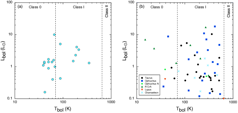
Figure 1: (a) $T_{\rm bol}$-$L_{\rm bol}$ diagram of the eDisk sample sources. (b) $T_{\rm bol}$-$L_{\rm bol}$ diagram of the protostars with $d<200~{}pc$ and $L_{\rm bol}>0.1~{}L_{\odot}$. Two dashed vertical lines in each diagram indicate the boundaries between Class 0 and Class I (70 K; see Evans et al., 2009) and Class I and Class II (650 K; see Evans et al., 2009).

Table 1: eDisk sample

Source name	Alternative name	ICRS R.A.	ICRS Dec.	Class	Distance	$T_{\rm bol}$	$L_{\rm bol}$		Ref.
		(h m s)	(d m s)		(pc)	(K)	($L_{\odot}$)
L1489 IRS	IRAS 04016+2610	04:04:42.85	+26:18:56.3	I	146	213	3.4	1
IRAS 04166+2706		04:19:42.50	+27:13:36.0	0	156	61	0.40	2
IRAS 04169+2702		04:19:58.45	+27:09:57.1	I	156	163	1.5	2
IRAS 04302+2247	Butterfly star	04:33:16.50	+22:53:20.4	I	160	88	0.43	1,3,4
L1527 IRS	IRAS 04368+2557	04:39:53.91	+26:03:09.8	0	140	41	1.3	5,6
Ced110 IRS4	IRAS 11051-7706	11:06:46.44	–77:22:32.2	0	189	68	1.0	7
BHR71 IRS2		12:01:34.09	–65:08:47.36	0	176	39	1.1	8
BHR71 IRS1	IRAS 11590–6452	12:01:36.81	–65:08:49.22	0	176	66	10	8
IRAS 15398-3359	B228	15:43:02.24	–34:09:06.8	0	155	50	1.4	9,10,11
GSS30 IRS3	SMM J162622-24225	16:26:21.72	–24:22:50.7	0	138	50	1.7	12
Oph IRS43	YLW 15	16:27:26.7	–24:40:52.3	I	137	193	4.1	13
IRAS 16253-2429		16:28:21.6	–24:36:23.4	0	139	42	0.16	10,14
Oph IRS63	IRAS 16285-2355	16:31:35.7	–24:01:29.6	I	132	348	1.3	10,12
IRAS 16544–1604	CB 68	16:57:19.64	–16:09:23.9	0	151	50	0.89	10
R CrA IRS5N	CrA-20	19:01:48.46	–36:57:14.7	0	147	59	1.4	10
R CrA IRS7B	SMM 1B	19:01:56.42	–36:57:28.4	I	152	88	5.1	9
R CrA IRAS 32	IRAS 18595-3712	19:02:58.67	–37:07:35.9	0	150	64	1.6	9
TMC-1A†	IRAS 04365+2535	04:39:35.2	+25:41:44.4	I	137	183	2.3	6
B335†	IRAS 19347+0727	19:37:0.89	+07:34:10.0	0	165	41	1.4	15

Note. — ^† For these sources, we used only ALMA archival data without new observations. Some of the archival data we used have slightly different phase centers from those shown in this table (see Table 6). Column 1: Target name. Column 2: Alternative common name also used in previous works. Column 3: Right ascension of the observation phase center in the International Celestial Reference System (ICRS). Column 4. Declination of the observation phase center in ICRS. Column 5. Evolutionary stage classification based on $T_{\rm bol}$. Column 6. Distance to the target based on recent estimations from Gaia measurements. Column 7: Bolometric temperature re-derived from the newly compiled SED. See Appendix A. Column 8: Bolometric luminosity re-derived from the newly compiled SED. See Appendix A. Column 9: Reference for the distance estimations.

References. — 1. Roccatagliata et al. (2020); 2. Krolikowski et al. (2021); 3. Galli et al. (2018); 4. Luhman (2018); 5. Kenyon et al. (1994); 6. Zucker et al. (2019); 7. Galli et al. (2021); 8. Voirin et al. (2018); 9. Galli et al. (2020); 10. Zucker et al. (2020); 11. Dzib et al. (2018); 12. Ortiz-León et al. (2018); 13. Ortiz-León et al. (2017); 14. de Geus et al. (1989); 15. Watson (2020)

All of the selected sources have complete spectral energy distributions (SEDs) measured from the near-infrared to submillimeter that are compiled in Appendix A. Based on those SEDs we re-derived their bolometric temperatures ($T_{\rm bol}$) and luminosities ($L_{\rm bol}$) also utilising the most recent distances from Gaia measurements listed in Table 3.1. Note that none of the 19 targets were detected with Gaia directly due to their embedded natures, but distances to nearby sources, presumably related to the same star-forming complexes, were typically estimated based on Gaia observations and provided the distance estimates quoted in literature. The final sample comprises 12 Class 0 and 7 Class I protostars and represents various evolutionary stages of protostars with a roughly uniform distribution of $L_{\rm bol}$ and $T_{\rm bol}$ (Figure 1a). For comparison purposes, Figure 1b shows the same $T_{\rm bol}$-$L_{\rm bol}$ diagram, but for the 56 protostars with $d<$200 pc and $L_{\rm bol}>0.1~{}L_{\odot}$ discussed above, except for two sources with unreasonably high $T_{\rm bol}$, indicating that the final 19 protostars reasonably represent the nearby and relatively bright protostars.

3.2 Observations

Observations of the eDisk program using the ALMA 12 m array in band 6 were conducted from April 2021 to July 2022. We aimed to achieve high angular resolutions of $\sim$0$.\!\!^{\prime\prime}$04, corresponding to $\sim$6 au at a distance of 140 pc. Such high angular resolution is necessary for us to investigate substructures of embedded disks and make direct comparisons with previous maps of Class II disks obtained at similar angular resolutions, such as those obtained by DSHARP or ODISEA.

The correlator was configured to observe both 1.3 mm continuum emission as well as CO ($J=2-1$) isotopologues and other lines providing additional information about the physical and chemical structures of the gas on the scales of the circumstellar disks surrounding the embedded protostars. Baseband 1 of the correlator was configured in the lower sideband with 4 spectral windows (spw) to include our primary molecular lines, C¹⁸O (2–1), ¹³CO (2–1), and SO ($6_{5}-5_{4}$), at a velocity resolution of $\sim$0.17 km s^-1. The ¹²CO (2–1) emission was included in baseband 4 in the opposite sideband to study protostellar outflows. The bandwidth of baseband 4 was set to be 937.5 MHz to secure the continuum bandwidth, and as a result, the velocity resolution of the ¹²CO data is 4 times worse than that of the C¹⁸O data. The remaining two basebands are located in the upper and lower sidebands, respectively, with the maximum bandwidth of 1875 MHz. While these two basebands were adopted for the 1.3 mm continuum emission, the central frequency of baseband 2 was adjusted to incorporate as many important molecular lines as possible, such as CH₃OH, SiO, DCN, H₂CO, and $c$-C₃H₂. Even though the velocity resolution of these observations, $\sim$1.3 km s^-1, is not ideal to study the kinematics from these molecular transitions, their detection can still provide useful constraints on circumstellar structures based on, e.g. the integrated intensities. All the major emission lines observed in our observations are listed in Table 2.

In order to achieve an angular resolution of $\sim$0$.\!\!^{\prime\prime}$04, the C43-8 antenna configuration was adopted for our observations, providing long baselines up to $\sim$12.6 km. In addition to the C43-8 antenna configuration, the C43-5 antenna configuration was also adopted to cover shorter baselines with a minimum of $\sim$15 m. This additional antenna configuration covering shorter baselines is crucial for us to investigate relatively extended structures up to $\sim 2{{}^{\prime\prime}}-3{{}^{\prime\prime}}$ in the envelopes surrounding our sampled protostars. We should note that a large fraction of the emission from the envelopes around the sampled protostars is still filtered out in our observations. However, this missing flux has less impact on the main objectives of the eDisk program focusing on dust and gas on the scales of the disks in the vicinity of the protostars. The Field of View (FoV) of the 12 m array at the observed frequency is $\sim 26{{}^{\prime\prime}}$. Logs of the observations are provided in Appendix B (see Table 5).

For two sources in our sample, TMC-1A and B335, comparable observations were obtained with ALMA prior to our eDisk program and we collected those data from the ALMA archive. In addition, due to scheduling constraints only short baseline data were obtained for Oph IRS 63 as a part of eDisk. Hence we relied on ALMA archival observations of Oph IRS 63 for long baseline data. The information on the ALMA archival data we use in the eDisk program is summarized in Appendix B (see Table 6).

Table 2: Main molecular lines covered in the spectral setups for the eDisk program

Rest frequency	Molecule	Transition	Velocity resolution	Note
(GHz)			(km s-1)
Baseband 2 (216.8125–218.6875 GHz)
217.10498	SiO	$5-4$	1.35	outflows, shocks
217.23860	DCN	$3-2$	1.35	envelopes (cold gas)
217.82204†	$c$-C3H2	$6_{0,6}-5_{1,5}$	1.34	envelopes (UV irradiated regions)
217.82215†	$c$-C3H2	$6_{1,6}-5_{0,5}$	1.34	envelopes (UV irradiated regions)
217.94005	$c$-C3H2	$5_{1,4}-4_{2,3}$	1.34	envelopes (UV irradiated regions)
218.16044	$c$-C3H2	$5_{2,4}-4_{1,3}$	1.34	envelopes (UV irradiated regions)
218.22219	H2CO	$3_{0,3}-2_{0,2}$	1.34	high density gas, temperature tracer
218.44006	CH3OH	$4_{2}-3_{1}$ $E$	1.34	envelopes, outflows
218.47563	H2CO	$3_{2,2}-2_{2,1}$	1.34	high density gas, temperature tracer
Baseband 1, spw 0 (218.730773–218.789367 GHz)
218.76007	H2CO	$3_{2,1}-2_{2,0}$	0.17	high density gas, temperature tracer
Baseband 1, spw 3 (219.531063–219.589657 GHz)‡
219.56035	C18O	2–1	0.17	envelopes, disks
Baseband 1, spw 2 (219.920143–219.978737 GHz)
219.94944	SO	$6_{5}-5_{4}$	0.17	high density gas, shocks
Baseband 1, spw 1 (220.350703–220.409297 GHz)‡
220.39868	13CO	2–1	0.17	disks, envelopes, outflows
Baseband 4 (230.09125–231.02875 GHz)
230.53800	12CO	2–1	0.63	outflows, envelopes, disks
Baseband 3 (233.3125–235.1875 GHz)
Mostly for the 1.3 mm continuum emission

Note. — $\dagger$ These two lines are blended. $\ddagger$ In the DDT observations, spw 1 and spw 3 in the baseband 1 were swapped, and the frequency range of the spw 3 in the DDT observations was set at 220.369383–220.427977 GHz.

4 Data reduction

4.1 Detailed procedure

The eDisk data were all calibrated using the ALMA calibration pipeline packaged with the Common Astronomy Software Application (CASA) (McMullin et al., 2007) version 6.2.1 and pipeline version 2021.2.0.128. After delivery, the data were restored to a calibrated state running scriptForPI.py in the same CASA version that the calibration pipeline ran with. For four sources (BHR71 IRS1/IRS2, IRAS 04166+2706, and IRAS 04169+2702), there were Execution Blocks (EBs) that were given a QA0 status of ‘semi-pass’ (see Table 5 in Appendix B), which in the case of these datasets was because of excessive phase decorrelation during the observations. For those we downloaded the raw data and ran the ALMA calibration pipeline manually to inspect the datasets and determine if they could be salvaged using self-calibration. The QA0 semi-pass data that are used in the final images are denoted in the Observing Logs included in Appendix B.

Outside of standard calibration, we needed to perform additional processing to improve the S/N of the continuum data through self-calibration, to remove the continuum emission from the line data, and to combine data taken in two configurations in order to achieve the balance between flux recovery and angular resolution needed to achieve the science goals of the project. Nearly all of the eDisk targets were sufficiently bright that images created using the standard ALMA calibration were dynamic range limited, meaning that the images were not reaching the thermal noise limit, and were instead limited by phase and/or amplitude variations during the science target observations. To both combine the two configurations, self-calibrate, continuum subtract, and image the data, we constructed a set of semi-interactive scripts for each target. Our methodology was based on the DSHARP data reduction procedure (Andrews et al., 2018) with substantial modification. One particular choice we made was to operate on each measurement set individually for calculation and application of phase and amplitude gain solutions and not concatenate our data to a single measurement set. This avoids issues that can be encountered when operating on concatenated measurement sets within various CASA tasks; for example, interpolation of gain solutions between distinct observations that might be far apart in time, spectral window numbers being offset, and possible issues with combined metadata to name a few. Many of the issues with concatenated measurement sets can be worked around, but we avoid the known issues and the possible unknown issues by operating on individual measurement sets. The scripts used for each source are provided at http://github.com/jjtobin/edisk.

The reduction procedure starts with the construction of a spectrally-averaged continuum dataset. We identified line-free regions of the individual spectral windows to include in the continuum dataset in two ways: first, we made use of the cont.dat file produced by the ALMA imaging pipeline, and edits to the continuum ranges in that file were made if necessary, based on inspection of the hif_findcont weblog. Second, we manually flagged the spectral lines that are expected to be present in all datasets regardless of whether they were already included in the cont.dat file. We then translated these frequency ranges defined in the kinematic local standard of rest frame (LSRK) to the channel ranges for each EB and flagged those channels. Then the separate spws from each EB were spectrally averaged individually. The four high-resolution spws were averaged over 480 channels and the three low-resolution spws were averaged 60 channels, resulting in $\sim$30 MHz channels, approximating the spectral resolution of the low-spectral resolution (time domain mode; TDM) of the ALMA correlator.

We next checked the relative flux density scaling of each individual EB using their azimuthally-averaged visibility amplitude data. To do this, we first imaged each EB individually and shifted the brightest source in the image to the phase center using the CASA task fixvis. We then computed the azimuthally-averaged visibility amplitudes for each EB, plotted them together, and computed the average scale factors between each EB. The scale factors were estimated between the minimum overlapping uv-distance out to 800 k$\lambda$; this outer uv-distance was chosen to avoid a possibility that decorrelation at longer baselines could significantly impact the scale factors. The offsets were typically at the 10–15% level between EBs and we scaled each EB to the ‘best’ EB which was judged by having the least amount of scatter in its data. Thus, our goal was a relative flux normalization of all the EBs, given that we were not improving on the overall flux density scale accuracy. We also note that there is possibility that some scale factors include intrinsic source variability in addition to calibration differences. While the ALMA Technical Handbook indicates that the accuracy of the flux density scale is expected to be $\sim$5%, the scaling that we have had to apply to datasets indicates that the flux density scale can have uncertainties up to the rescaling factors that we apply to the data.. The scale factor applied to each EB is provided in Appendix C.

There were some cases where this flux normalization could not be performed at this stage due to decorrelation, which caused the visibility amplitude profile of one or more EBs to have a different behavior as a function of uv-distance than others. In those cases, we did not determine scale factors at this stage, but we completed the self-calibration steps that followed and determined the scale factors after self-calibration. We then re-ran the whole procedure from the start, applying these scale factors a priori; we referred to this as the ‘two-pass’ method. The ‘two-pass’ method was applied to Oph IRS43, IRAS 04166+2706, IRAS 04169+2702, and BHR71 IRS1 and IRS2. The relative scaling of each EB was then applied to the continuum datasets that did not have the brightest source shifted to the phase center because the unshifted data were what we ultimately used in the self-calibration process.

Following flux normalization of each EB we began the self-calibration process. For the combined processing of the compact and extended configuration data, we first self-calibrated the compact configuration data and then we self-calibrated the pre-self-calibrated compact configuration data with the extended configuration data. Self-calibration was performed using the data that did not have the phase center shifted. It was not necessary to align our data prior to self-calibration because the time difference between observations was less than 1 year and all the long baseline data, where proper motion would have the greatest effect, were all taken within a 3 month time period. We create our model for self-calibration using the data from all the measurement sets; however, it is only the calculation and application of the phase and amplitude gain solutions that happen on a per-measurement set basis.

To prepare for self-calibration, we first calculated a ranked list of reference antennas for each EB, equally weighing the amount of flagging on a particular antenna and its geometric position within the array. Following this step, we made an initial image using all the continuum datasets to determine the peak S/N of the image from standard calibration; the creation of all images during the self-calibration process made use of the tclean auto-multithresh algorithm (Kepley et al., 2020) to automatically create clean masks for deconvolution. Following the generation of this initial image, we analyzed the scan lengths within an observation and determined calibration solution intervals that most evenly divide a scan by the number of integrations per scan. This approach will avoid the uneven division of scans which can result in some solutions being calculated from significantly less data. The list of solution intervals to attempt always includes a solution that spans the length of an EB, referred to as ‘inf_EB’ where gaincal is run with the parameter combine=‘scan,spw’. The ‘inf_EB’ solution interval corrects systematic effects, in particular, antenna position offsets that translate to systematic phase offsets between the calibrator and science target. Then for shorter solution intervals, we are correcting the atmospheric phase variations. We include an ‘inf’ solution, where the ‘scan’ setting is removed from the gaincal parameters and solutions break at scan boundaries, then for shorter solutions, we divide the median scan length by 2 and all subsequent solution intervals divide the previous interval by 2 until the final solution interval of ‘int’ (one integration) is reached.

Then for each solution that is to be attempted, we also determine the clean depths in terms N$\times$ $\sigma$ to use for each solution interval in order to progressively clean deeper during each round of self-calibration. We begin with the assumption that we would trust features with intensities $>$ (Peak S/N)/15, which means that for a Peak S/N = 150, we would trust features $>$ 10$\sigma$. Note that these numbers are empirical, but small changes do not appreciably affect the outcome of self-calibration. So we divide the S/N of the initial image by 15 to obtain our starting clean threshold, and decreased the thresholds for subsequent solution intervals logarithmically until the clean depth is equivalent to 3$\sigma$.

With a set of solution intervals to attempt and their accompanying clean thresholds, the self-calibration process begins. We collect all the model creation with tclean, calibration solution generation with gaincal, application of the calibration solutions with applycal, and checking the outcome of a self-calibration iteration with tclean into a single Python function to simplify to process. We always use the combine=‘spw’ parameter in gaincal to use all the available bandwidth for self-calibration and we use the parameter interp=’linearPD’ which will scale the phase solutions with frequency to compensate for the fact that the optimal phase solutions will be different between the low and high frequency end of the bandwidth.

At the start of each self-calibration iteration, the self-calibrated data from the previous iteration (corrected data column) is split out into a new measurement set such that each self-calibration solution interval is incremental upon the previous iteration. We compare the image S/N before self-calibration and after self-calibration of each iteration is applied to ensure that the S/N is increasing. We do this by running tclean again but using the self-calibration model that was created at the start of a self-calibration iteration as the startmodel for tclean. This approach enables us to effectively determine the improvement in S/N just due to the gain corrections derived from that model. When the image S/N increases within an iteration, we consider that iteration successful, if the S/N decreases, that iteration has failed and we consider the last successful iteration as the final self-calibration iteration. The above steps consider phase-only self-calibration and we do attempt amplitude self-calibration (solving for amplitude and phase simultaneously) following the phase-only self-calibration using the same criteria for success or failure of amplitude self-calibration. Following the completion of self-calibration for the successful solution intervals, the self-calibrated data for each EB are saved to new measurement sets and are considered the final continuum data.

Once self-calibration is completed on the continuum data, we process the line data. First, we apply the flux normalization to each full measurement set using the scaling factors derived from the continuum. Then we apply the self-calibration solutions to the full measurement sets for each EB. However, the S/N improvement for the line data are typically not significant because the line data are not dynamic range limited like the continuum. For each EB, we apply all the gain tables for each successful self-calibration iteration, which is necessary because each table is incremental, so applying the full correction requires all the tables. Once self-calibration solutions are applied, we subtract continuum emission from the line data using the uvcontsub task. To subtract the continuum data, we select the line-free regions of the data that will have their continuum data fitted and subtracted. To select the frequency ranges to fit, we select the complement of the frequency ranges that were flagged to produce the continuum dataset, that is the line-free regions of the bandwidth. Following uv continuum subtraction, we have the final spectral line data set and it is ready for imaging.

We first create the continuum images using tclean and the auto-multithresh algorithm to create the clean masks. Then we create images using Briggs weighting, for the robust parameters of -2, -1, -0.5, 0, 0.5, 1, and 2 in order to compare the features present with different weighting. We also created images using uv-tapering, to reduce the influence of the long baselines and bring out larger-scale structure, and we created tapered images with the tapers starting at 1000, 2000, and 3000 k$\lambda$ and used robust parameters of 1 and 2. The typical synthesized beam size for the robust=0.5 images was $\sim$0$.\!\!^{\prime\prime}$05. The images for most sources use 6000 pixels with a pixel size of 0$.\!\!^{\prime\prime}$003; however, some sources require image sizes of $\sim$14000 in order to include sources toward the edge of the primary beam.

Then we create the spectral line images for each line listed in Table 2. We typically created images using Briggs weighting with robust values of 0.5 and 2, and uv-tapering starting at 2000 k$\lambda$. The resulting images have synthesized beams of $\sim$0$.\!\!^{\prime\prime}$1 and $\sim$0$.\!\!^{\prime\prime}$15 for the two robust values and applied tapering, respectively. The tapering was essential for the spectral line images because the surface brightness sensitivity was otherwise too low at the native resolution of the data to detect the spectral lines with high S/N. The spectral line images typically used 4000 pixels and a pixel size of 0$.\!\!^{\prime\prime}$01. The spectral line images were all created with velocity-defined channels around the spectral lines of interest using their associated rest frequencies (Table 2).

We then save the non-primary beam corrected images (flat noise), the primary beam corrected images, the final clean mask, and the primary beam response for each individual image. As such, there are $\sim$52 images created per target when all the combinations of robust parameters, lines, and tapering are considered. The images presented in this overview paper and subsequent papers from the eDisk program are selected based on the balance between resolution and sensitivity, and also the structures discussed.

4.2 Jorsater & van Moorsel effect

Recently it has been pointed out that data imaged with the clean algorithm may suffer systematic errors of the flux scale due to the so-called Jorsater & van Moorsel (JvM) effect (Jorsater & van Moorsel (1995); see, in particular, Czekala et al. (2021)). The reason for this is that the dirty beams in the CLEAN processes deviate from the used Gaussian restoring beams. As discussed in Czekala et al. (2021), the JvM effect is more significant when data taken from different antenna configurations are combined like in the case of the eDisk program. The impact due to the JvM effect to the flux scales of our eDisk maps differs from source to source: maps with more extended diffuse emission are more impacted by the JvM effect. However, it has also been pointed out that the correction method to fix the flux scale issue, implemented by Czekala et al. (2021), may artificially manipulate the noise levels of maps after the correction (Casassus & Cárcamo, 2022). As the main discussions of the first set of papers from eDisk are based primarily on the morphology of maps and velocity structure of molecular emission rather than the flux scale of maps, we did not apply any correction to our maps in this overview paper and the related first set of papers.

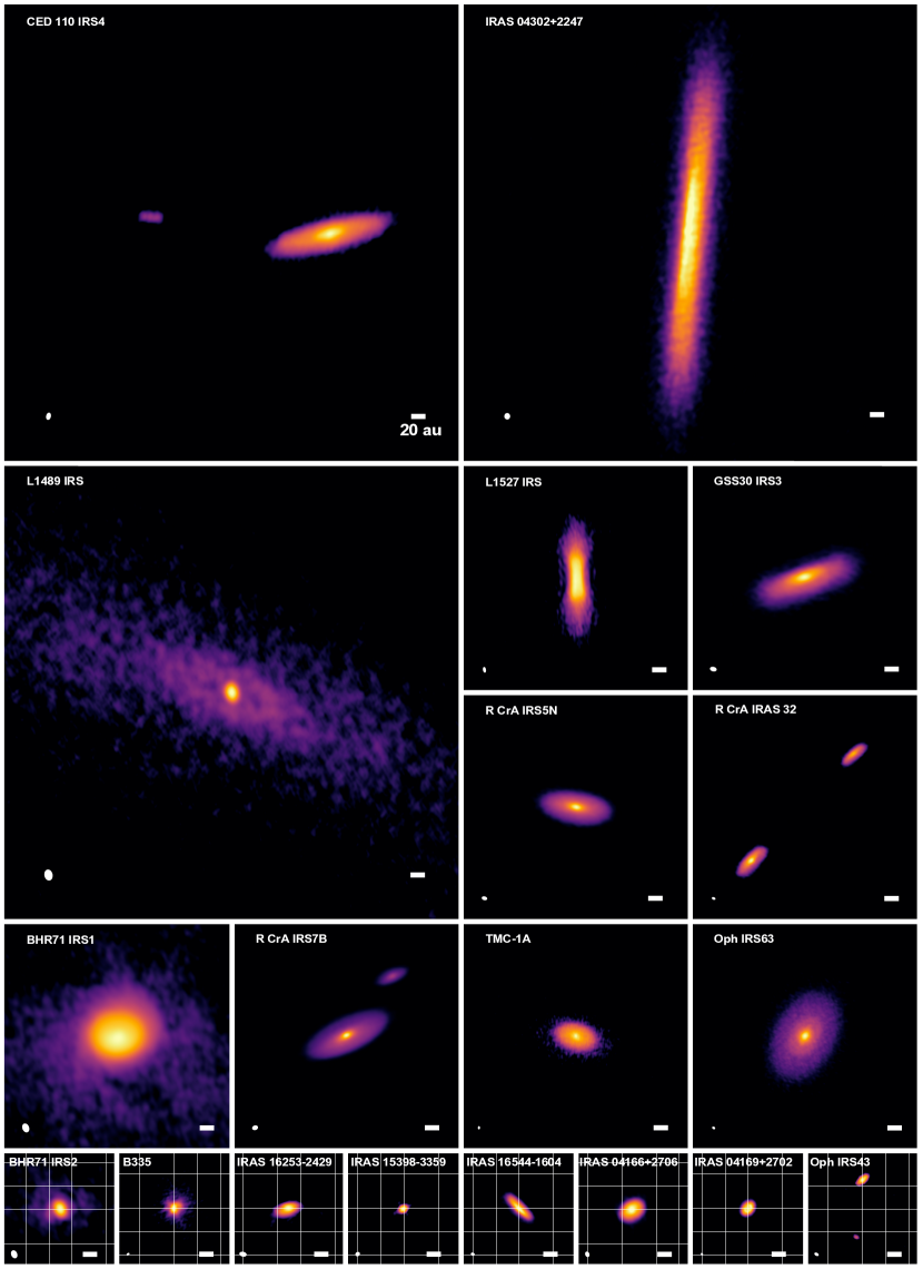
Figure 2: Gallery of the continuum maps obtained in the eDisk program. All maps are shown in the same linear scale (large panels: 640 au $\times$ 640 au, medium panels: 320 au $\times$ 320 au, small panels: 160 au $\times$ 160 au). All the maps are shown in individual asinh-stretch intensity scales, except for IRAS 04169+2702 that is shown in a linear intensity scale. All the map centers are source positions listed in Table 3, except for Ced110 IRS4, R CrA IRAS 32, and Oph IRS43, where the map centers are shifted from the source positions by (0$\hbox{$.\!\!^{\prime\prime}$}{75}$, 0$\hbox{$.\!\!^{\prime\prime}$}{0}$), ($-0\hbox{$.\!\!^{\prime\prime}$}{5}$, $0\hbox{$.\!\!^{\prime\prime}$}{5}$), and (0$\hbox{$.\!\!^{\prime\prime}$}{0}$, $-0\hbox{$.\!\!^{\prime\prime}$}{3}$), respectively to show the binary. The beam size and the scale of 20 au are shown at the bottom left and right corners in each panel, respectively.

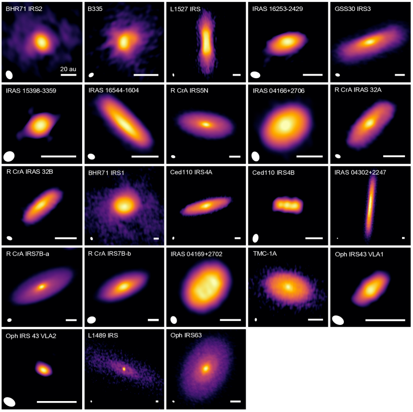
Figure 3: Enlarged continuum images. Images of IRAS 04302+2247 and L1489 IRS are not enlarged from those in Figure 2. The intensity scales are the same as those in Figure 2 except for the 4 companions. All the map centers are source positions listed in Table 3. Images are presented in an order of T_bol listed in Table 3.1. The beam size and the scale of 20 au are shown at the bottom left and right corners in each panel, respectively.

5 First results

In this section, we present the first results of our eDisk program, an overview of the observations of the 1.3 mm continuum for the sample of sources as well as an example of analysis of the C¹⁸O 2–1 emission toward R CrA IRS7B. The structures of embedded disks can be traced well in the 1.3 mm dust continuum emission, while C¹⁸O is the key molecular line to study the kinematics of the gas on small scales, e.g. searches for the presence of Keplerian disks and estimates of the dynamical masses of the central protostars. In this sense, the presentation here provides a glance at the type of scientific results that can be obtained from the eDisk data. More details of the first results about each targeted source can be found in a series of subsequent papers (see the references in Table 3).

5.1 Continuum emission

We present representative maps of the continuum images obtained in the eDisk program on the same spatial scale in Figure 2. The same continuum images but enlarged are also presented in Figure 3. Robust parameters used to create these continuum images and their angular resolutions are shown in Table 3. The rms noise level of these continuum maps is $\sim$25 $\mu$Jy beam^-1 on average. Continuum emission is clearly detected at all source positions, and four out of the 19 sources also show continuum emission arising from companions; three of them, i.e., Ced110 IRS4, R CrA IRS7B, and R CrA IRAS 32, are newly found to be binaries in our observations. These newly found binaries are named based on the IAU convention; Ced110 IRS4A and Ced110 IRS4B, R CrA IRS7B-a and R CrA IRS7B-b, and R CrA IRAS 32A and R CrA IRAS 32B.

All the continuum emission images are spatially resolved, exhibiting elongated structures. These elongated structures strongly suggest that the dust continuum traces disks around the targeted sources. Note that for some sources envelope contamination may still play a role for both dust and gas emission: to assess that more detailed radiative transfer modeling will be needed on a source-by-source basis. The extent of the continuum emission, measured through 2-D Gaussian fittings and listed in Table 3, varies significantly from source to source; L1489 IRS has the largest emission with an angular extension of $\sim 3\hbox{$.\!\!^{\prime\prime}$}{9}\times 1\hbox{$.\!\!^{\prime\prime}$}{3}$, while the companion of Oph IRS43 (VLA 2) is the most compact, marginally resolved ($2\sigma$) with an angular extent $\sim 0\hbox{$.\!\!^{\prime\prime}$}{019}\times 0\hbox{$.\!\!^{\prime\prime}$}{016}$. We note that some of the continuum emissions were not well fitted with 2-D Gaussian, suggesting that the extents of the emissions provided in Table 3 for those sources may not reflect their actual extents. In such a sense, the extents of the continuum emissions provided here should be considered as a quick reference of their extents measured by a simple procedure. More accurate measurements of the extents of the dust emissions through more sophisticated methods will be presented in future papers. A comparison between the extents of the continuum emission from the different sources and their bolometric temperatures is shown in Figure 4. In agreement with the systematic studies of protostars in Orion with the VLA (Tobin et al., 2020), no clear correlation between size and evolutionary stage is seen - although the two largest disks in our sample are both associated with Class I protostars (L1489 IRS and IRAS 04302+2247). Most of the disks in the eDisk sample are smaller than about 100 au but we caution that these are estimates of the sizes of the dust disks and that the gas disks may be larger as it is often inferred for more evolved disks (see, e.g., Miotello et al., 2022).

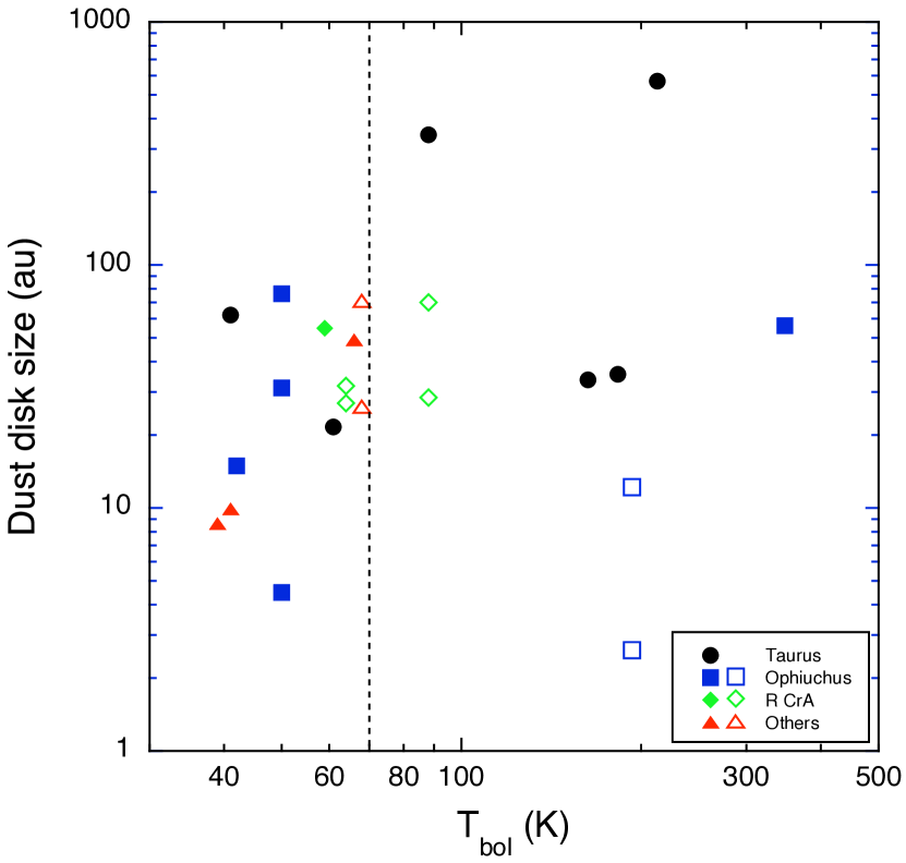
Figure 4: Dust disk size in diameter is plotted as a function of bolometric temperature of their central protostellar system. Sources located in different regions are shown in different symbols. Open symbols show the 4 binary systems (Ced110 IRS4A/B, Oph IRS43 VLA1/VLA2, R CrA IRS7B-a/b, and R CrA IRAS 32A/B). The vertical dashed line shows the boundary between Class 0 and I sources.

From a comparison between the major and minor axes of the continuum emission, the inclination of the system can be also estimated on the assumption that the continuum emission is a vertically thin disk. We find that 7 out of 19 sources, excluding companions, have inclination angles of more than 70 degrees (see Table 3), roughly consistent with the expectation from a random distribution. We caution that the estimate of the inclination is a lower limit to the true inclination because the disks have most likely some vertical thickness. Still, these are different from most Class II disks that have been observed at high angular resolution to date which tend to be more face-on (Andrews et al., 2018; Cieza et al., 2021). Figure 5 shows a comparison between the inclination angle and the bolometric temperature, demonstrating no correlation between them. This suggests that the disk inclination has less impact on our classification of the 19 protostellar systems based on the bolometric temperature even though it was also suggested that higher inclination angles of disks could misclassify protostars as Class 0 sources (Tamura et al., 1996; Nakazato et al., 2003; Tobin et al., 2008; Fischer et al., 2017). We also note that some of the continuum structures show relatively high brightness temperatures of more than 100 K. Such high brightness temperature may suggest that the detected continuum emission is at least partially optically thick. Basic physical parameters of the continuum emission are summarized in Table 3. We note that statistical errors are not given in this table because the actual uncertainties of these measurements are more likely determined by systematic errors, such as the flux calibration error and the gain calibration error.

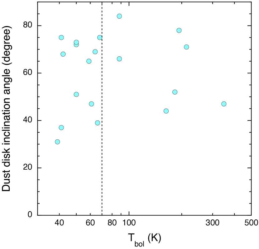
Figure 5: Dust disk inclination angle is plotted as a function of bolometric temperature of their systems. Four binary companions (Ced110 IRS4B, Oph IRS43 VLA2, R CrA IRS7B-b, and R CrA IRAS 32B) are excluded. The vertical dashed line shows the boundary between Class 0 and I sources.

Table 3: Physical parameters of continuum emission

Source name	ICRS R.A.	ICRS Dec.	Robust	$\theta_{\rm b}$, $PA_{\rm b}$	Extent, PA	Peak $I_{\nu}$, $T_{\rm b}$	$F_{\nu}$	inc.	Ref.
	(h m s)	(d m s)		(mas,°)	(mas,°)	(mJy beam-1, K)	(mJy)	(°)
L1489 IRS	04:04:43.080	+26:18:56.12	1	105$\times$78, 12	3913$\times$1283, 66	5.4, 21	91	71	1
IRAS 04166+2706	04:19:42.505	+27:13:35.83	0	49$\times$37, 22	138$\times$94, 122	9.6, 133	71	47	2
IRAS 04169+2702	04:19:58.477	+27:09:56.82	0	48$\times$37, 21	216$\times$156, 139	4.3, 64	101	44	3
IRAS 04302+2247	04:33:16.499	+22:53:20.23	0.5	55$\times$50,3	2149$\times$239,175	1.1, 14	183	84	4
L1527 IRS	04:39:53.878	+26:03:09.43	–0.5	56$\times$29, 9	444$\times$114, 2	4.3, 69	139	75	5
Ced110 IRS4A	11:06:46.369	–77:22:32.88	0	54$\times$35, –13	376$\times$99, 104	5.8, 79	80	75	6
Ced110 IRS4B	11:06:46.772	–77:22:32.76	0	54$\times$35, –13	138$\times$41, 85	0.38, 9	2.0	73	6
BHR71 IRS2	12:01:34.008	–65:08:48.08	0.5	70$\times$50, 23	49$\times$42, 68	8.7, 65	14	31	7
BHR71 IRS1	12:01:36.476	–65:08:49.37	0.5	72$\times$53, 22	279$\times$215, 98	26, 170	384	39	7
IRAS 15398-3359	15:43:02.232	–34:09:06.96	-0.5	43$\times$36, –56	29$\times$18, 117	5.9, 93	7.9	51	8
GSS30 IRS3	16:26:21.715	–24:22:51.09	0	68$\times$45, 77	550$\times$169, 109	6.4, 56	124	72	9
Oph IRS43 VLA1	16:27:26.906	–24:40:50.81	–1	46$\times$30, 61	89$\times$18, 136	3.3, 62	11	78	10
Oph IRS43 VLA2	16:27:26.911	–24:40:51.40	–1	46$\times$30, 61	19$\times$16, 131	0.88, 20	1.1	32	10
IRAS 16253-2429	16:28:21.615	–24:36:24.33	0	73$\times$48, 78	107$\times$40,113	5.1, 40	12	68	11
Oph IRS63	16:31:35.654	–24:01:30.08	0	34$\times$25, 57	426$\times$292, 149	5.8, 170	280	47	12
IRAS 16544–1604	16:57:19.643	–16:09:24.02	0	36$\times$27, 69	207$\times$60, 45	4.1, 103	52	73	13
R CrA IRS5N	19:01:48.480	–36:57:15.39	0.5	50$\times$30,75	374$\times$157, 81	5.5, 94	99	65	14
R CrA IRS7B-a	19:01:56.420	–36:57:28.66	0	54$\times$42, –73	462$\times$174, 115	18, 195	339	68	15
R CrA IRS7B-b	19:01:56.385	–36:57:28.11	0	54$\times$42, –73	187$\times$75, 115	5.4, 63	36	66	15
R CrA IRAS 32A	19:02:58.722	–37:07:37.39	–0.5	35$\times$23, 67	212$\times$78, 135	4.9, 153	80	69	16
R CrA IRAS 32B	19:02:58.642	–37:07:36.39	–0.5	35$\times$23, 67	180$\times$58, 132	3.2, 102	44	72	16
TMC-1A†	04:39:35.202	+25:41:44.22	0	32$\times$21, –1	259$\times$159, 76	5.0, 187	184	52	17
B335†	19:37:00.900	+07:34:09.81	0	27$\times$19, –54	60$\times$48, 163	5.0, 243	29	37	17

Note. — ^†For these sources, we used only ALMA archival data without new observations. Column 1: target names. Column 2: Right ascension of the continuum emission measured with single 2-D Gaussian fittings. For L1489 IRS 2-D Gaussian fittings with two-component were performed because single 2-D Gaussian fittings did not provide a solution. Column 3: Declination of the continuum emission measured with single 2-D Gaussian fittings. For L1489 IRS 2-D Gaussian fittings with two-component were performed because single 2-D Gaussian fittings did not provide a solution. Column 4: Robust parameter used to create the continuum image shown in Figures 2 and 3. Column 5: synthesized beam FWHM and position angle of the representative map shown in Figure 2. Column 6: Beam deconvolved size and position angle of the continuum emission measured with single 2-D Gaussian fittings. For L1489 IRS 2-D Gaussian fittings with two-component were performed because single 2-D Gaussian fittings did not provide a solution. Column 7: Peak intensity of the continuum emission and its brightness temperature estimated with the full Plank function. Column 8: Integrated flux density of the continuum emission measured with single 2-D Gaussian fittings. For L1489 IRS 2-D Gaussian fittings with two-component were performed because single 2-D Gaussian fittings did not provide a solution. Column 9: Inclination angle of the continuum emission estimated from the ratio of the major and minor axes of the continuum emission listed in the column 5. Column 10: References from the eDisk program. 1. Yamato et al. (2023); 2. Phuong et al. (2023); 3. Han et al. (2023); 4. Lin et al. (2023); 5. van ’t Hoff et al. (2023); 6. Sai et al. (2023); 7. Gavino et al. (2023); 8. Thieme et al. (2023); 9. Santamaría-Miranda et al. (2023); 10. Narayanan et al. (2023); 11. Aso et al. (2023); 12. Flores et al. (2023); 13. Kido et al. (2023); 14. Sharma et al. (2023); 15. Ohashi et al. (2023); 16. Encalada et al. (2023); 17. This work

When we carefully inspect the continuum maps, it is found that some of them show ring-like structures that can be visually identified by naked eye. The most obvious source is L1489 IRS. Oph IRS63 also weakly shows ring-like structures. More details of the continuum maps obtained in the eDisk program will be presented in subsequent papers. Ring-like structures in continuum emission around these two sources have been suggested by previous studies as well (Ohashi et al., 2022; Segura-Cox et al., 2020) although our map of L1489 IRS seems to show ring-like structures more clearly than in the previous work (Ohashi et al., 2022). The continuum emission around IRAS 04169+2702 seems to show a bean-like structure with brighter emission on its southwest side, which could also be a ring-like structure. We should stress that a more detailed and systematic analysis of continuum emission is definitely required to identify their substructures, including those that cannot be visually identified by the naked eye, as will be discussed in a forthcoming paper. Nevertheless, the first analysis on the observations suggests that continuum emission around our Class 0/I sample does not show very sharp ring or spiral structures that are often seen in Class II continuum disks (e.g., DSHARP, ODISEA). This striking difference will be discussed in more detail in Sec. 6.1. On the other hand, several disk continuum images show brightness asymmetries, particularly along their minor axes. IRAS 04302+2247, GSS 30 IRS3, IRAS 16253-2429, IRAS 16544–1604, R CrA IRS7B-a, R CrA IRAS 32A, and R CrA IRAS 32B show clear asymmetry that can be identified by eye, while asymmetry can be also identified with more careful inspection of continuum intensity distributions for some additional sources, such as L1527 IRS. For these sources showing brightness asymmetries, the geometric centers of the continuum emission derived from single 2-D Gaussian fittings listed in Table 3 are shifted from their actual continuum peak positions. The possible origin of the brightness asymmetry is discussed in Section 6.1.

5.2 C¹⁸O 2–1

The C¹⁸O 2–1 emission is also detected toward all 19 sources in our sample. Here, we show the C¹⁸O emission detected in one of our sources, R CrA IRS7B, as an example of what can be seen toward the eDisk targets.

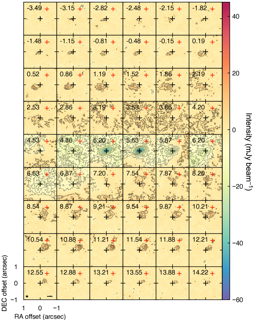
Figure 6: C¹⁸O channel maps with a velocity resolution of 0.334 km s^-1 (two channels combined) in R CrA IRS7B. Solid contours are drawn from 3$\sigma$ to 15$\sigma$ every 3$\sigma$ for positive emissions, while dashed contours are drawn from -3$\sigma$ to -15$\sigma$ every -3$\sigma$ and less every -5$\sigma$. 1$\sigma$ is 1.2 mJy beam^-1. The center of each channel map is the position of R CrA IRS7B-a shown in Table 3. The black and red crosses in each panel indicate the positions of IRS7B-a and IRS7B-b, respectively. The beam size and a scale bar of 50 au are shown at the bottom-left and the bottom-right corners in the bottom-left panel.

Lindberg et al. (2014) have carried out ALMA observations of IRS7B in Band 7 at an angular resolution of $\sim 0\hbox{$.\!\!^{\prime\prime}$}{4}$ and detected continuum emission and several molecular lines, including C¹⁷O 3–2. Both continuum and C¹⁷O emission have extended structures elongated in the southeast to northwest direction. The C¹⁷O emission also shows a clear velocity gradient along the elongation, which was interpreted as Keplerian rotation (Lindberg et al., 2014). Although a systemic velocity of 6.2 km s^-1 was adopted for the analysis of the velocity structures of C¹⁷O in Lindberg et al. (2014), we adopt $\sim$6.0 km s^-1 as the systemic velocity of IRS7B in this paper (see more details below).

C¹⁸O 2-1 was detected at more than 3$\sigma$ in the LSR velocity range between $-$3.15 km s^-1 and 14.22 km s^-1 at an angular resolution of $\sim 0\hbox{$.\!\!^{\prime\prime}$}{13}\times 0\hbox{$.\!\!^{\prime\prime}$}{11}$ as shown in Figure 6. Note that the velocity resolution of the C¹⁸O data shown here is $\sim$0.33 km s^-1, which is double the original velocity resolution to achieve a higher sensitivity. Since the systemic velocity of this system is $\sim$6 km s^-1 (see Sec. 6.2), LSR velocities smaller and larger than 6 km s^-1 correspond to blue- and red-shifted, respectively. At higher blue-shifted velocities ($V_{\rm LSR}=-3.15$ to 2.86 km s^-1) and red-shifted velocities ($V_{\rm LSR}=8.20$ to 14.22 km s^-1), C¹⁸O is mainly detected on the southeast side and the northwest side of IRS7B-a within $\sim$0$.\!\!^{\prime\prime}$5, respectively. At lower blue-shifted ($V_{\rm LSR}=3.19$ to 4.20 km s^-1) and red-shifted velocities ($V_{\rm LSR}=7.20$ to 7.87 km s^-1), more extended C¹⁸O emission is detected within the field of $2{{}^{\prime\prime}}\times 2{{}^{\prime\prime}}$, demonstrating that our observations can also trace extended emission as well. At velocities close to the systemic velocity, absorption of C¹⁸O is detected. In particular, very deep absorption is seen at the position of IRS7B-a at $V_{\rm LSR}$ between 5.20 and 5.87 km s^-1. The extent of the deep absorption is almost the same as that of the continuum emission associated with IRS7B-a, suggesting that the deep absorption is due to cold, foreground C¹⁸O emission against the bright continuum emission. Compact and weak C¹⁸O emission is detected at the position of IRS7B-b at several channels of red-shifted velocities, such as $V_{\rm LSR}=9.21$ and 11.21 km s^-1, and also absorption at $V_{\rm LSR}=5.20$ and 5.53 km s^-1. The absorption at the position of IRS7B-b may be also due to cold foreground C¹⁸O against the continuum emission associated with IRS7B-b.

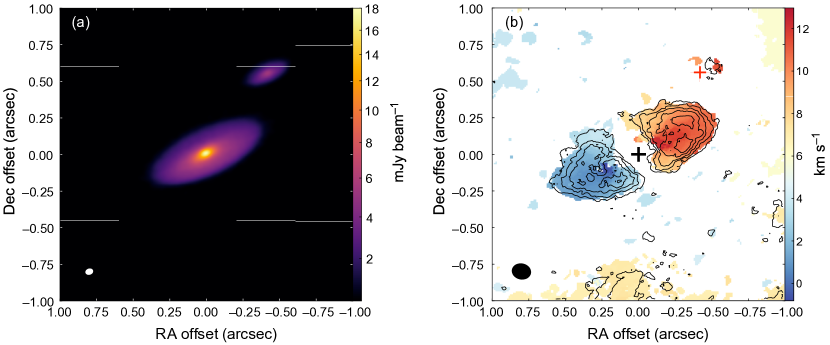
Figure 7: (a) Continuum emission map in IRS7B. IRS7B-a is located at the center of the map, while IRS7B-b is located to the northwest side of IRS7B-a. The beam size is shown in the bottom-left corner as the white ellipse. (b) C¹⁸O moment 0 map shown in contour and moment 1 map shown in color. The moment 0 map was created by integrating emission having intensity more than 3$\sigma$ (1 $\sigma$ = 1.2 mJy beam^-1) in the velocity range of -3.15 km s^-1 to 14.22 km s^-1 to avoid the influence of the deep absorption features. The moment 1 map was created over the same velocity range as the moment 0 map with the emission having an intensity more than 5$\sigma$. The contours of the moment 0 map are drawn every 2$\sigma$ from 3$\sigma$ (1$\sigma$ = 2.9 mJy beam^-1km s^-1). The black and red crosses indicate the positions of IRS7B-a and IRS7B-b, respectively. The beam size is indicated in the bottom-left corner with the black ellipse.

To investigate the overall distribution and velocity structures of C¹⁸O around IRS7B-a, moment 0 and 1 maps of IRS7B are shown in Fig. 7b. For comparison, the continuum map of IRS7B is also shown in Fig. 7a. The moment 0 map shows two emission components with semi-elliptic shapes, one located to the southeastern side of IRS7B-a and the other located on the northwestern side of IRS7B-a, forming a disk-like structure divided into two along its minor axis as a whole. The C¹⁸O disk-like structure is basically similar to that seen in the continuum associated with IRS7B-a, although it extends slightly larger than the continuum emission, suggesting that C¹⁸O probably traces gas associated with the protoplanetary disk around IRS7B-a, but further investigation of the kinematics of C¹⁸O is required for us to have a firm conclusion (see below). Although both continuum and C¹⁸O show similar disk-like structures, their intensity distributions are quite different, e.g., C¹⁸O is stronger in outer parts of the disk-like structure and it gets weaker toward the position of IRS7B-a, where the continuum emission shows a peak. This discrepancy would be most likely due to absorption of the warm continuum emission by colder C¹⁸O gas.

The moment 1 map presented in Figure 7b shows a velocity structure of the C¹⁸O emission having blue-shifted velocities with respect to the systemic velocity of $\sim$6 km s^-1 on the southeastern side and red-shifted velocities on the northwestern side. This clear velocity gradient along the major axis of the disk-like structure is naturally interpreted as rotation. The nature of the velocity structures can be investigated further with a position-velocity (PV) diagram cutting along the major axis, as discussed in Sec. 6.2. The diagram shows that the velocity of C¹⁸O increases toward the position of IRS7B-a, a clear sign of differential rotation. Further discussions on the nature of the rotation are presented in Section 6.2.

6 Discussion

6.1 Substructures and asymmetry of continuum emission

When we compare our continuum maps from Fig. 2 with those toward Class II sources, from, e.g., the DSHARP and ODISEA programs, the absence of clear ring or spiralstructures identifiable by the naked eye with few exceptions is remarkable. The noticeable difference between protostars and Class II sources could suggest that substructures are not well developed in the embedded phase yet, and they could be quickly formed when Class 0/I protostars evolve into Class II sources. Interestingly, the two sources, L1489 IRS and Oph IRS 63 showing visually identified ring-like structures and another source, IRAS 04169+2702, possibly showing a ring-like structure in the eDisk sample are all Class I protostars. In addition, two protostars previously found to have ring-like structures in their continuum maps are also Class I protostars (WL 17 and GY 91). Note that substructures found in dust continuum around GY 91 are less sharpe than those seen around Class II sources (see Sheehan & Eisner, 2018; Cieza et al., 2021) while WL 17 does show a sharp ring-like structure (Sheehan & Eisner, 2017). Although seven sources from the Orion VANDAM survey exhibit relatively clear ring structures, these ring structures could be due to close binary formation (Sheehan et al., 2020).

We should note, however, that a reason behind the lack of obvious sharp substructures in continuum emission around the Class 0/I protostars could also be that the continuum emission at 225 GHz may be optically thick. In fact, some of the continuum emission observed in the eDisk program may be optically thick as indicated by their higher brightness temperatures (see Table 3). To address this possibility, it will be necessary to observe continuum emission at lower frequencies, where dust continuum emission is expected to be optically thinner. One of the sources in the eDisk sample, L1527 IRS, has been observed in 7 mm continuum with VLA, finding no clear gaps (Sheehan et al., 2022).

We should also note that some of the disk structures seem to be more inclined (see Table 3), particularly as compared with Class II disks observed at high angular resolution to date, which could make substructures more difficult to be observed in disks around our sample. In addition, some of the continuum emissions are also more compact, and our angular resolution may not be high enough to detect substructures. More detailed analyses and discussions of substructures in the continuum emission, including the visibility analysis, will be presented in forthcoming papers.

In contrast to substructures, several of the target sources show brightness asymmetries, particularly along their minor axes (see Figure 3). A possible explanation for these brightness asymmetries along the minor axes might come from a geometrical effect, namely, the far-side of a highly inclined disk with a finite vertical thickness is brighter than the near-side. Such a near-far side brightness asymmetry is an indication that the dust has yet to completely settle onto the disk midplane. In more edge-on systems such as HH 212, the non-settled dust produces a dark lane near the mid-plane sandwiched between two brighter features (Lee et al., 2017; Lin et al., 2021). In contrast to embedded disks, Class II disks rarely show any asymmetry along their minor axes (e.g., Andrews et al., 2018; Long et al., 2019). The difference could suggest that dust is not quite settled in the embedded phase but quickly settles as embedded disks evolve into Class II disks.

6.2 Identifying Keplerian rotation

Table 4: Results of the best fitting to the C¹⁸O PV diagram

Parameter	Unit	Description	Best fit value
			Edge	Ridge
$p_{\rm in}$		Power of the fitting function	0.61$\pm$0.04	0.51$\pm$0.01
$V_{\rm sys}$	km s-1	systemic velocity	6.04$\pm$0.04	6.00$\pm$0.02
Mass	$M_{\sun}$	Dynamical mass of the central star	3.21$\pm$0.04	2.06$\pm$0.02

In addition to investigating substructures in continuum emission, another important purpose of the eDisk program is to identify Keplerian rotation around our target protostars. Here we discuss the case of R CrA IRS7B-a as an example showing how we identify Keplerian rotation.

One of the methods to identify Keplerian rotation, which is also adopted by the eDisk program, is fitting to position-velocity (PV) diagrams. Our fitting process includes two independent methods. One method uses the ridge in 1D intensity profiles along the positional axis (the velocity axis) at a given velocity (position). The other method uses the outer edge in the 1D intensity profiles. We call the former the ridge method, while we call the latter the edge method. In each method, PV diagrams are fitted with a power-law function. The function is a single- or double-power function, which is defined with a power-law index, $p_{\rm in}$. The systemic velocity, $v_{\rm sys}$, is also included as a free parameter in the fitting process. More details of the fitting method and process are explained in Appendix D.

As was shown in Section 5.2, the C¹⁸O emission in R CrA IRS7B-a shows a velocity gradient along its disk-like elongated structure centered at the position of R CrA IRS7B-a, suggestive of rotation. The C¹⁸O PV diagram cutting along the major axis of the dust emission around R CrA IRS7B-a presented in Figure 8 shows that the rotation can be described as differential rotation, and it is fitted in both the edge and ridge methods described above. The fitting results are presented in Table 4. For demonstration purposes, only fittings with a single-power law function are presented here. Both edge and ridge fittings with a single power-law show that $p_{\rm in}$ is close to 0.5, suggesting that the rotation can be explained as Keplerian rotation. The dynamical mass of the central protostar was estimated to be $\sim 3.2~{}M_{\sun}$ with the edge method, while it was estimated to be $\sim 2.1~{}M_{\sun}$ with the ridge method. As explained in Appendix D, the actual dynamical mass of the central star is considered to be between $\sim 2.1~{}M_{\sun}$ and $\sim 3.2~{}M_{\sun}$. Discussions on further details of the Keplerian disk around R CrA IRS7B-a are beyond the scope of this overview paper, and they will be presented in the subsequent paper.

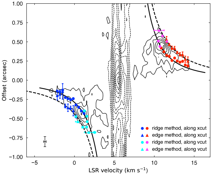
Figure 8: C¹⁸O position-velocity diagram of R CrA IRS7B-a with a velocity resolution of 0.334 km s^-1. Contours are drawn from 3$\sigma$ to 15$\sigma$ in every 2$\sigma$ for positive emission, while dashed contours are drawn from -3$\sigma$ to -15$\sigma$ in every -3$\sigma$ and less every -5$\sigma$. 1$\sigma$ is 1.2 mJy beam^-1. Cicles and triangles show data points obtained through the ridge and edge methods, respectively, while the solid and dashed curves represent fitting results obtained through the ridge and edge methods, respectively. Different colors show data points obtained along different direction: blue and red show data points obtained along the position axis (xcut), while cyan and magenta represent data points obtained along the velocity axis (vcut).

7 Data Release

As one of ALMA large programs, the eDisk program will release a suite of data products that have legacy values for the community. The released data sets, which will be available at https://almascience.org/alma-data/lp/edisk, include (1) CASA scripts and associated python modules used to calibrate and image the data; (2) calibrated visibility data from each execution block, including those from the ALMA archive; (3) continuum images created from combined visibility data with a robust value of 0.5; (4) line cube images created from combined visibility data with a robust value of 0.5; (5) fits file of the primary beam for each image mentioned above. These released data sets enable the community to reproduce all the images presented in this paper and forth coming papers.

8 Summary

This article has provided an introduction to the ALMA large program, eDisk, including the background of the program, the sample selection of the 19 Class 0/I protostars, the ALMA observations at Band 6, and the data reduction processes. The first look results of the 1.3 mm continuum emission detected around all the 19 targets for the eDisk program and C¹⁸O 2–1 emission detected around one of the 19 targets, R CrA IRS7B, are presented to demonstrate what kind of results we would expect to see in the eDisk program.

All the continuum emission is spatially resolved at angular resolutions of $\sim 0\hbox{$.\!\!^{\prime\prime}$}{04}$, revealing elongated disk-like structures. The detected continuum emission is considered to trace embedded disks around the sampled Class 0/I protostars although they could also partially arise from inner parts of the envelopes surrounding the protostars. More importantly, the continuum emission does not show any sharp ring-like or spiral-like structures with high contrast, which are often seen in Class II disks. This could suggest that substructures are formed in disks quickly when Class 0/I protostars evolve to Class II sources or otherwise that high optical depth of dust emission may obscure such features. Note that some of the continuum emission show more compact or inclined disk-like structures, which could prevent us from finding substructures there. Asymmetries in the brightness distributions along minor axes seen by eye for some sources may also reflect the dust optical thickness and orientations of the disks.

C¹⁸O 2–1 emission detected in R CrA IRS7B-a also shows an elongated disk-like structure similar to that seen in its dust continuum emission. There is a clear velocity gradient along the elongation. The analysis of the velocity structures in the PV-diagram cutting along the elongation suggests that the velocity gradient seen in the C¹⁸O elongation can be explained as Keplerian rotation with a central dynamical mass of 2.1-3.2 $M_{\sun}$.

The first results here already demonstrate the great potential of the data from the eDisk program. A set of accompanying papers go into more detail about the first results for individual sources setting the stage for future more synergistic studies. These analyses will provide new, important constraints on these pivotal stages in the formation and early evolution of protostars and their disks.

Appendix A Spectral energy distributions

The spectral energy distributions (SEDs) for the sources in the eDisk sample are shown in Fig. 9. The majority of the spectral data for the sources were compiled from the NASA/IPAC Infrared Science Archive (IRSA) database. We searched toward the position of each source and include flux values and errors from catalog positions within 5^′′ of the source coordinates. These include data from Herschel (PACS and SPIRE), Spitzer (IRAC and MIPS), the SCUBA bolometer on the JCMT, WISE/NeoWISE, and Akari. In addition, Spitzer IRS spectra were available from the CASSIS database for some sources, which have also been included in the plots. In the eDisk sample, BHR71 IRS1 and IRS2 constitute a binary system and GSS30 IRS3 is part of a triple system each separated by of order 10^′′ from their companions. Hence, in particular, the long wavelength flux points include unresolved emission from all companions and the flux values from IRSA require deconvolution before they are used for SED fits. For BHR71 IRS1 and IRS2, the deconvolved values are taken from Tobin et al. (2019), whereas for GSS30 IRS3, the deconvolved values over 50 $\mu$m are taken from Je et al. (2015). For the closer binaries/multiples in the sample, the bolometric temperature and luminosities refer to the overall values for the systems.

For each source, we perform spline-fits to the SEDs and use these to calculate the $L_{\textrm{bol}}$ and $T_{\textrm{bol}}$ of the sources. The $L_{\textrm{bol}}$ is computed by integrating all the points on the spline fits with the trapezoid function of the scipy package. The $T_{\textrm{bol}}$ for each of the sources are calculated using the average frequency of the SED fits following the methods in Myers & Ladd (1993).

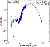
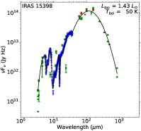
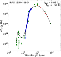
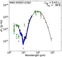
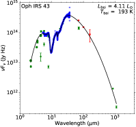
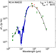
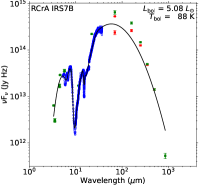
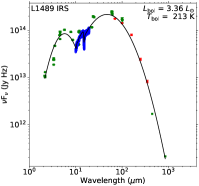
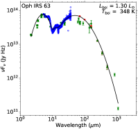
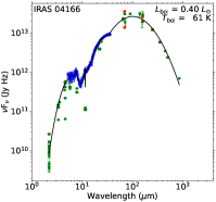
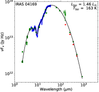
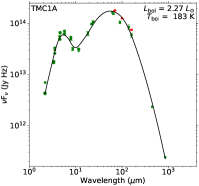
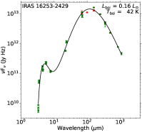
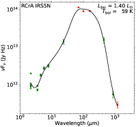
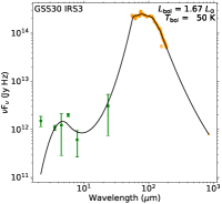
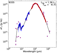
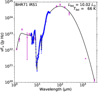
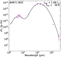
Figure 9: Spectral energy distributions from the near-infrared to millimeter ranges of the eDisk sources. Photometric data and spectroscopic data are shown in filled squares and empty circles, respectively. Flux data taken from the IRSA database are shown in green and Spitzer IRS spectra are shown in blue. Herschel PACS/SPIRE data are shown in red. Deconvolved GSS30 IRS3 data taken from Je et al. (2015) are shown in orange. B335 flux data shown in purple are taken from Evans et al. (2023) and Herschel PACS/SPIRE spectral data shown in red are taken from Green et al. (2016). Photometry data for BHR71 IRS1 and IRS2 data taken from Tobin et al. (2019) are shown in magenta. The black line represents the spline fit of the SED values used to calculate each source’s $L_{\textrm{bol}}$ and $T_{\textrm{bol}}$.

Appendix B Observation logs

Here we present a table of the observation logs for the eDisk program (see Table 5). In addition, we present a table of observation logs for the ALMA archival data we used in the eDisk Program (see Table 6).

Appendix C Scale factors

Here we present a scale factor we applied to each EB in Table 7. See more details in Sec. 4.

Appendix D Fittings to position-velocity diagrams

One of the methods to identify Keplerian rotation, which is also adopted by the eDisk program, is fitting to position-velocity (PV) diagrams. Such an analytic approach has advantages of the lower computational cost and a simpler process than model fitting to visibility data including radiative transfer with ten or more free parameters (Sheehan et al., 2019), although the robustness of fitting the PV diagram would be less than that of fittings to visibility data due to fitting in the image vs. uv-plane and the reduced spatial dimension. The analytic method also enables us to focus on a specific quantity, such as the central stellar mass, without complicated parameter degeneracy. Our fitting process includes two independent methods. One method uses the ridge in 1D intensity profiles along the positional axis (the velocity axis) at a given velocity (position). This ridge method is demonstrated in previous observational studies (Ohashi et al., 2014; Aso et al., 2017; Yen et al., 2017; Sai et al., 2020) with a discussion about its potential problems (Yen et al., 2013; Aso et al., 2015), as well as in a study using synthetic observations of a magnetohydrostatic (MHD) simulation of protostellar evolution (Aso & Machida, 2020). The other method uses the outer edge in the 1D intensity profiles. This edge method was developed using an MHD simulation of protostellar evolution (Seifried et al., 2016) and is used in previous observational studies as well (e.g., Alves et al., 2017; Reynolds et al., 2021). The advantage and disadvantage of each method are debatable. For example, Maret et al. (2020) reported that, depending on the spatial resolution, the ridge method can underestimate the central stellar mass by $\sim 30\%$, while the edge method can overestimate it by a factor of $\sim 2$. For this reason, we regard the radius, or central stellar mass, derived from the ridge method as the lower limit and the one derived from the edge method as the upper limit.

In the eDisk program, the fitting process with the edge and ridge methods is implemented through the public Python package pvanalysis in SLAM (Aso & Sai, 2023). The process is composed of two main steps: obtaining the edge and ridge points in a PV diagram and fitting the obtained points with a power-law function. First, the edge and ridge radii are obtained in the 1D intensity profile along the positional axis at the given velocity (xcut). The edge radius is defined as the outermost position with a given threshold level ($3\sigma$ in this paper) of emission. The uncertainty of the edge radius is calculated from the emission gradient and the observational noise level. The ridge radius is defined as the intensity-weighted mean position in the 1D profile or the center derived from the Gaussian fitting. This fitting also calculates an uncertainty of the ridge radius from the observational noise level. Similarly, the edge and ridge velocities are obtained in the 1D profile along the velocity axis at a given position (vcut). Then, in each of edge and ridge methods, the xcut points at velocities higher than a “middle” velocity and the vcut points at radii larger than a “middle” radius are combined as the final pairs of $(r,v)$. The middle velocity and radius are determined from the closest pair of points between the xcut and vcut, as explained in Aso & Machida (2020) in more detail. Note that 1D intensity profiles along only one direction (position or velocity) would be enough to obtain the edge and ridge points if a PV-diagram is mainly elongated along the velocity or positional axis, respectively.

Second, the obtained pairs of $(r,v)$ are fitted with a power-law function, in the edge and ridge methods separately. The function is a single- or double-power function as follows:

$$v={\rm sign}(r)\ v_{b}\left(\frac{|r|}{r_{b}}\right)^{-p}+v_{\rm sys},$$ (D1)

$$p=p_{\rm in}\ \ {\rm if}\ \ |r|<r_{b}\ \ {\rm else}\ \ p_{\rm in}+dp,$$ (D2)

where $v_{b}$ is the velocity at the radius of $r_{b}$, $p_{\rm in}$ is the power-law index, $dp$ is the difference of the index between the inner and outer parts, and $v_{\rm sys}$ is the systemic velocity. $dp$ is limited to be $\geq 0$ to produce a steeper or the same index outside $r_{b}$, such as the inner Keplerian rotation versus the outer rotation where the angular momentum is conserved. For the single-power fitting, $v_{b}$ is fixed at a middle value and $dp=0$. Equation D2 provides a function of radius, defined here as $V_{\rm fit}(r)$. When $dp\geq 0$, the inverse function of velocity $R_{\rm fit}(v)$ can be defined. Using these functions, $\chi^{2}$ to be minimized is defined as

$$\chi^{2} = \sum_{i~{}\rm for~{}xcut}\left(r_{i,{\rm obs}}-R_{\rm fit}(v_{i,{\rm obs}})\right)/\sigma^{2}_{i,{\rm obs}}$$ (D3)

$$+\sum_{j~{}\rm for~{}vcut}\left(v_{j,{\rm obs}}-V_{\rm fit}(r_{j,{\rm obs}})\right)^{2}/\sigma^{2}_{j,{\rm obs}},$$

where $\sigma$ is the uncertainty of each radius/velocity obtained above.

The power-law fitting provides the pair of $(r_{b},v_{b})$. From this pair, the central stellar mass can be calculated as $M_{*}=v_{b}^{2}r_{b}/G/\sin^{2}i$, where $G$ is the gravitational constant and $i$ is an inclination angle. The inclination angle is often estimated from the aspect ratio of the associated continuum emission or independent modeling of the associated outflow, which is beyond the scope of this fitting with PV diagrams. If the power-law index $p_{\rm in}$ is significantly different from the Keplerian index 0.5, the estimated $M_{*}$ does not have the meaning of the central stellar mass.

=15mm

Table 5: eDisk observing logs (2019.1.00261.L and 2019.A.00034.S)

Source name	UTC Date	Config.	Baselines	Nant	Elev.	PWV	Calibrators	Check source
			(m)		(deg.)	(mm)
L1489 IRS	2021 Aug 20 07:43	C43-8	59–9934	43	31.7	0.7	J0423–0120, J0423–0120, J0357+2319	J0401+2110
	2021 Aug 20 09:29	C43-8	59–9934	46	40.0	0.5	J0510+1800, J0510+1800, J0357+2319	J0401+2110
L1489 IRS, L1527 IRS	2021 Dec 03 03:02	C43-5	15–2617	46	40.4	1.8	J0510+1800, J0510+1800, J0438+3004	J0435+2532
	2021 Dec 16 03:29	C43-5	15–1917	42	37.2	2.3	J0510+1800, J0510+1800, J0438+3004	J0435+2532
	2022 Jul 03 12:58	C43-5	15–1301	42	36.3	1.3	J0237+2848, J0237+2848, J0438+3004	J0418+3801
IRAS 04166+2706, IRAS 04169+2702	2021 Sep 30 05:20†	C43-8	70–11886	44	$\cdots$	0.73	J0238+1636, J0238+1636, J0433+2905	J0429+2724
	2021 Oct 01 05:22†	C43-8	70–10803	45	$\cdots$	1.77	J0238+1636, J0238+1636, J0438+3004	J0440+2728
	2021 Oct 18 04:32†	C43-8	46–8983	43	$\cdots$	0.70	J0238+1636, J0238+1636, J0438+3004	J0435+2532
	2021 Oct 24 07:20	C43-8	46–8983	45	35.2	0.26	J0510+1800, J0510+1800, J0438+3004	J0440+2728
	2022 Jul 3 13:15	C43-5	15-1301	41	39.5	1.40	J0510+1800, J0510+1800, J0438+3004	J0435+2532
	2022 Jul 3 14:26	C43-5	15-1301	41	37.4	1.49	J0510+1800, J0510+1800, J0438+3004	J0435+2532
IRAS 04302+2247	2021 Sep 30 08:48	C43-8	70-11886	45	$\cdots$	0.9	J0510+1800, J0510+1800, J0426+2327	J0425+2235
	2021 Oct 01 06:54	C43-8	70–10803	43	$\cdots$	2.1	J0510+1800, J0510+1800, J0426+3227	J0425+2235
	2021 Oct 01 08:31	C43-8	70-10803	45	42.1	1.8	J0510+1800, J0510+1800, J0426+2327	J0425+2235
	2021 Dec 01 03:40	C43-5	15-3638	48	43.8	1.0	J0510+1800, J0510+1800, J0426+2327	J0425+2235
L1527 IRS	2021 Oct 14 08:26	C43-8	91-11469	42	35.5	0.5	J0510+1800, J0510+1800, J0438+3004	J0433+2905
	2021 Oct 15 06:01	C43-8	91-8983	41	39.3	0.8	J0510+1800, J0510+1800, J0438+3004	J0433+2905
	2021 Oct 15 07:51	C43-8	91-8983	41	38.2	0.7	J0510+1800, J0510+1800, J0438+3004	J0433+2905
Ced 110 IRS4	2021 Apr 24 01:30	C43-5	15-1397	45	35.3	1.4	J1107-4449, J1107-4449, J1058-8003	$\cdots$
	2021 Oct 04 13:05	C43-8	70-10803	42	35.2	0.3	J0519-4546, J0519-4546, J1058-8003	J1224-8313
	2021 Oct 20 10:58	C43-8	46-8983	47	33.7	0.7	J0519-4546, J0519-4546, J1058-8003	J0942-7731
	2021 Oct 20 12:24	C43-8	46-8983	44	35.4	0.7	J1427-4206, J1427-4206, J1058-8003	J0942-7731
BHR 71 IRS1, BHR 71 IRS2	2021 May 04 00:26	C43-5	15-2517	44	47.3	1.6	J1107-4449, J1107-4449, J1147-6753	J1206-6138
	2021 May 09 01:26	C43-5	15-2517	44	47.3	1.4	J1107-4449, J1107-4449, J1147-6753	J1206-6138
	2021 Oct 14 14:48†	C43-8	91-8983	41	$\cdots$	0.88	J1427-4206, J1427-4206, J1147-6753	J1145-6954
	2021 Oct 15 13:13	C43-8	91-8983	43	46.7	0.5	J1427-4206, J1427-4206, J1147-6753	J1145-6954
	2021 Oct 16 12:18†	C43-8	46-8983	42	$\cdots$	0.66	J0635-7516, J0635-7516, J1147-6753	J1145-6954
	2021 Oct 19 14:34	C43-8	91-8547	41	47.3	0.7	J1427-4206, J1427-4206, J1147-6753	J1145-6954
	2021 Oct 20 13:57†	C43-8	46-8983	43	$\cdots$	0.76	J1427-4206, J1427-4206, J1147-6753	J1145-6954
IRAS 15398-3359	2021 May 06 03:56	C43-5	15-2517	45	74.9	1.2	J1337-1257, J1337-1257, J1610-3958	J1523-3338
	2021 Aug 09 22:34	C43-8	70-8282	39	77.9	0.7	J1337-1257, J1337-1257, J1534-3526	J1523-3338
	2021 Aug 13 23:41	C43-8	70-8282	42	66.3	1.7	J1517-2422, J1517-2422, J1534-3526	J1523-3338
	2021 Oct 20 15:28	C43-8	46-8983	43	59	0.8	J1427-4206, J1427-4206, J1534-3526	J1536-3151
GSS 30 IRS3, IRAS 16253-2429	2021 Oct 05 22:14	C43-8	70-11614	46	49.7	3.5	J1517-2422, J1517-2422, J1633-2557	J1650-2943
	2021 Oct 26 19:22	C43-8	63-8547	45	71.1	3.3	J1427-4206, J1427-4206, J1633-2557	J1642-2849
	2021 Oct 27 20:35	C43-8	63-8547	46	52.2	1.3	J1427-4206, J1427-4206, J1633-2557	J1642-2849
	2021 Oct 28 17:02	C43-8	63-8282	43	79.7	1.0	J1427-4206, J1427-4206, J1633-2557	J1642-2849
GSS 30 IRS3, IRAS 16253-2429, Oph IRS63	2022 Jun 14 04:13	C43-5	15-1301	42	70.3	0.3	J1517-2422, J1517-2422, J1700-2610	J1650-2943
	2022 Jun 15 00:45	C43-5	15-1301	43	62.8	0.5	J1517-2422, J1517-2422, J1700-2610	J1650-2943
Oph IRS 43	2021 May 26 07:32	C43-5	15-2280	42	$\cdots$	3.6	J1924-2914, J1924-2914, J1700-2610	J1642-2849
	2021 Jun 08 05:01	C43-5	15-2386	45	$\cdots$	0.6	J1517-2422, J1517-2422, J1700-2610	J1642-2849
	2021 Oct 10 22:11	C43-8	70-11469	44	47.1	1.8	J1517-2422, J1517-2422, J1633-2557	J1650-2943
	2021 Oct 19 21:37†	C43-8	46-8547	41	$\cdots$	1.59	J1924-2914, J1924-2914, J1633-2557	J1642-2849
	2021 Oct 25 19:14	C43-8	46-8547	46	73.5	1.5	J1427-4206, J1427-4206, J1633-2557	J1642-2849
IRAS 16544–1604	2021 Aug 24 01:21	C43-8	47-12594.5	50	56	0.4	J1924-2914, J1924-2914, J1653-1551	J1657-2004
	2021 Oct 04 22:48	C43-8	70-11614.8	45	48.7	0.6	J1924-2914, J1924-2914, J1653-1551	J1657-2004
	2021 Oct 05 20:59	C43-8	70–11614	46	72.3	3.1	J1517-2422, J1517-2422, J1653-1551	J1657-2004
	2022 Jun 14 03:11	C43-5	15-1301	42	81.6	0.3	J1517-2422, J1517-2422, J1733-1304	J1745-0753
R CrA IRS5N, R CrA IRAS 32	2021 May 04 10:17	C43-5	15-2517	42	$\cdots$	1.7	J1924-2914, J1924-2914, J1937-3958	J1839-3453
	2021 May 15 08:52	C43-5	15-2517	45	$\cdots$	1.0	J1924-2914, J1924-2914, J1937-3958	J1839-3453
	2021 Aug 18 04:20	C43-8	92-8282	40	45.8	0.3	J1924-2914, J1924-2914, J1839-3453	J1823-3454
	2021 Aug 22 04:13	C43-8	47-11614	49	44.1	0.3	J1924-2914, J1924-2914, J1839-3453	J1823-3454
	2021 Oct 01 01:30	C43-8	70-11614	45	45.1	1.5	J1924-2914, J1924-2914, J1839-3453	J1823-3454
	2021 Oct 02 23:25	C43-8	70-11614	43	67.6	0.7	J1924-2914, J1924-2914, J1839-3453	J1826-3650
R CrA IRS7B	2021 May 03 09:05	C43-5	15-1997	43	72.2	0.5	J1924-2914, J1924-2914, J1937-3958	J1839-3453
	2021 Aug 10 01:36	C43-8	59-8282	46	75.5	0.5	J1924-2914, J1924-2914, J1839-3453	J1823-3454
	2021 Aug 10 04:21	C43-8	59-8282	46	52.8	0.4	J1924-2914, J1924-2914, J1839-3453	J1823-3454

Note. — ^† QA0 was Semi-passed. Column 1: Observed source name included in each execution block. Column 2: Observation start time in UTC. Column 3: Antenna configulation. Column 4: Range of Baseline length. Column 5: Number of antennas used for observation. Column 6: Averaged elevation during observation. An entry of “$\cdots$” indicates no information was available for the averaged elevation. Column 7: Averaged precipitable water vapor (PWV) during observation. Column 8: from left to right, the quasars observed for calibrating the bandpass, amplitude scale and phase variations. Column 9: Checking the phase transfer. An entry of “$\cdots$” indicates no check source was observed for checking the phase transfer.

=15mm

Table 6: Observing logs of archival data used in the eDisk program

Source name	UTC Date	Config.	Baselines	Nant	Elev.	PWV	Calibrators	Check source	Program ID
			(m)		(deg.)	(mm)
Oph IRS 63	2015 Nov 01 18:49	C36-8/7	84–14969	41	71.2	1.4	J1517-2422, J1517-2422, J1625-2527	J1633-2557	2015.1.01512.S
	2015 Nov 08 14:09	C36-8/7	84–16196	42	50.9	0.57	J1517-2422, J1517-2422, J1625-2527	J1633-2557	2015.1.01512.S
	2017 Sep 18 23:42	C40-8/9	41–12145	43	43.5	1.5	J1517-2422, J1733-1304, J1625-2527	J1633-2557	2015.1.01512.S
TMC-1A	2015 Sep 20 06:47	C34-7/(6)	41–2270	35	37.2	1.76	J0510+1800, J0423-013, J0429+2724	$\cdots$	2013.1.01086.S
	2015 Oct 23 06:10	C36-8	84–16196	40	41	0.58	J0510+1800, J0510+1800, J0440+2728	J0433+2905	2015.1.01415.S♯
	2015 Oct 30 06:10	C36-8/7	84–16196	43	41	0.37	J0510+1800, J0510+1800, J0440+2728	J0433+2905	2015.1.01415.S♯
B335	2014 Sep 02 01:30	C34-6	33–1091	34	$\cdots$	1.1	J1751+0939, J1751+096, J1955+1358	$\cdots$	2013.1.00879.S
	2017 Oct 08 00:45	C43-10	41–16196	51	41.9	0.5	J2148+0657, J2148+0657, J1938+0448	J1929+0507	2017.1.00288.S§
	2017 Oct 21 00:21	C43-10	41–16196	49	36.7	1.2	J2134-0153, J2134-0153, J1938+0448	J1929+0507	2017.1.00288.S§
	2017 Oct 22 00:29	C43-10	41–16196	46	34.5	1.1	J2134-0153, J2134-0153, J1938+0448	J1929+0507	2017.1.00288.S§
	2017 Oct 26 23:59	C43-9	135–14851	47	36.3	0.7	J2000-1748, J2000-1748, J1938+0448	J1929+0507	2017.1.00288.S§
	2017 Oct 29 23:10	C43-9	113–13894	45	43.5	1.3	J2000-1748, J2000-1748, J1938+0448	J1929+0507	2017.1.00288.S§

Note. — ^♯The declination of the phase center for TMC-1A was 25:41:44.27 in this program. ^§The phase center for B335 was (19:37:00.894, 07:34:09.59) in this program. Column 1: Observed source name included in each execution block. Column 2: Observation start time in UTC. Column 3: Antenna configuration. Column 4: Range of Baseline length. Column 5: Number of antennas used for observation. Column 6: Averaged elevation during observation. An entry of “$\cdots$” indicates no information was available for the averaged elevation. Column 7: Averaged precipitable water vapor (PWV) during observation. Column 8: from left to right, the quasars observed for calibrating the bandpass, amplitude scale, and phase variations. Column 9: Checking the phase transfer. An entry of “$\cdots$” indicates no calibrator was observed for checking the phase transfer. Column 10: Program ID.

Table 7: Scale factors

Source name	UTC Date	Scale factor
L1489 IRS	2021 Aug 20 07:43	0.86
	2021 Aug 20 09:29	0.95
	2021 Dec 03 03:02	1.000
	2021 Dec 16 03:29	0.91
	2022 Jul 03 12:58	0.87
IRAS 04166+2706	2021 Sep 30 05:20†	1.000
	2021 Oct 01 05:22†	0.91
	2021 Oct 18 04:32†	0.87
	2021 Oct 24 07:20	0.86
	2022 Jul 3 13:15	0.93
	2022 Jul 3 14:26	0.94
IRAS 04169+2702	2021 Sep 30 05:20†	0.96
	2021 Oct 01 05:22†	0.86
	2021 Oct 18 04:32†	0.90
	2021 Oct 24 07:20	0.93
	2022 Jul 3 13:15	1.000
	2022 Jul 3 14:26	0.99
IRAS 04302+2247	2021 Sep 30 08:48	0.9
	2021 Oct 01 06:54	1.000
	2021 Oct 01 08:31	0.74
	2021 Dec 01 03:40	0.97
L1527 IRS	2021 Dec 03 03:02	1.18
	2021 Dec 16 03:29	1.13
	2022 Jul 03 12:58	0.92
	2021 Oct 14 08:26	0.95
	2021 Oct 15 06:01	0.96
	2021 Oct 15 07:51	1.000
Ced110 IRS4	2021 Apr 24 01:30	0.91
	2021 Oct 04 13:05	1.02
	2021 Oct 20 10:58	1.01
	2021 Oct 20 12:24	1.000
BHR71 IRS2	2021 May 04 00:26	0.82
	2021 May 09 01:26	1.000
	2021 Oct 14 14:48†	1.01
	2021 Oct 15 13:13	1.10
	2021 Oct 16 12:18†	1.14
	2021 Oct 19 14:34	1.14
	2021 Oct 20 13:57†	1.34
BHR71 IRS1	2021 May 04 00:26	1.04
	2021 May 09 01:26	1.000
	2021 Oct 14 14:48†	0.97
	2021 Oct 15 13:13	1.11
	2021 Oct 16 12:18†	1.13
	2021 Oct 19 14:34	1.20
	2021 Oct 20 13:57†	1.17
IRAS 15398-3359	2021 May 06 03:56	1.0
	2021 Aug 09 22:34	1.04
	2021 Aug 13 23:41	1.04
	2021 Oct 20 15:28	0.62
GSS30 IRS3	2021 Oct 05 22:14	1.0
	2021 Oct 26 19:22	0.92
	2021 Oct 27 20:35	1.000
	2021 Oct 28 17:02	1.07
	2022 Jun 14 04:13	0.87
	2022 Jun 15 00:45	0.86
Oph IRS43	2021 May 26 07:32	1.20
	2021 Jun 08 05:01	1.50
	2021 Oct 10 22:11	0.93
	2021 Oct 19 21:37†	0.95
	2021 Oct 25 19:14	1.000
IRAS 16253-2429	2021 Oct 05 22:14	0.71
	2021 Oct 26 19:22	0.68
	2021 Oct 27 20:35	0.88
	2021 Oct 28 17:02	0.76
	2022 Jun 14 04:13	0.99
	2022 Jun 15 00:45	1.000
Oph IRS63	2015 Nov 01 18:49‡	0.98
	2015 Nov 08 14:09‡	1.05
	2017 Sep 18 23:42‡	1.05
	2022 Jun 14 04:13	1.01
	2022 Jun 15 00:45	1.000
IRAS 16544–1604	2021 Aug 24 01:21	1.02
	2021 Oct 04 22:48	1.11
	2021 Oct 05 20:59	1.000
	2022 Jun 14 03:11	0.82
R CrA IRS5N	2021 May 04 10:17	1.03
	2021 May 15 08:52	1.00
	2021 Aug 18 04:20	0.99
	2021 Aug 22 04:13	0.96
	2021 Oct 01 01:30	1.000
	2021 Oct 02 23:25	0.96
R CrA IRS7B	2021 May 03 09:05	0.95
	2021 Aug 10 01:36	1.000
	2021 Aug 10 04:21	0.99
R CrA IRAS 32	2021 May 04 10:17	1.01
	2021 May 15 08:52	1.04
	2021 Aug 18 04:20	1.000
	2021 Aug 22 04:13	0.93
	2021 Oct 01 01:30	0.98
	2021 Oct 02 23:25	0.93
TMC-1A	2015 Sep 20 06:47‡	1.000
	2015 Oct 23 06:10‡	0.74
	2015 Oct 30 06:10‡	0.63
B335	2014 Sep 02 01:30‡	0.75
	2017 Oct 08 00:45‡	1.00
	2017 Oct 21 00:21‡	1.000
	2017 Oct 22 00:29‡	1.04
	2017 Oct 26 23:59‡	0.99
	2017 Oct 29 23:10‡	1.01

Note. — ^† QA0 was Semi-passed. ^‡ALMA archival data. Column 1: target names. Column 2: Observation start time in UTC. Column 3: Scale factor applied to each EB. The scale factor of the reference EB is shown as 1.000.

References

- Akiyama et al. (2016) Akiyama, E., Hasegawa, Y., Hayashi, M., & Iguchi, S. 2016, ApJ, 818, 158, doi: 10.3847/0004-637X/818/2/158
- ALMA Partnership et al. (2015) ALMA Partnership, Brogan, C. L., Pérez, L. M., et al. 2015, ApJ, 808, L3, doi: 10.1088/2041-8205/808/1/L3
- Alves et al. (2017) Alves, F. O., Girart, J. M., Caselli, P., et al. 2017, A&A, 603, L3, doi: 10.1051/0004-6361/201731077
- Andrews et al. (2016) Andrews, S. M., Wilner, D. J., Zhu, Z., et al. 2016, ApJ, 820, L40, doi: 10.3847/2041-8205/820/2/L40
- Andrews et al. (2018) Andrews, S. M., Huang, J., Pérez, L. M., et al. 2018, ApJ, 869, L41, doi: 10.3847/2041-8213/aaf741
- Ansdell et al. (2016) Ansdell, M., Williams, J. P., van der Marel, N., et al. 2016, ApJ, 828, 46, doi: 10.3847/0004-637X/828/1/46
- Artur de la Villarmois et al. (2019) Artur de la Villarmois, E., Jørgensen, J. K., Kristensen, L. E., et al. 2019, A&A, 626, A71, doi: 10.1051/0004-6361/201834877
- Aso et al. (2023) Aso, Y., Kwon, W., Ohashi, N., et al. 2023, ApJ, submitted
- Aso & Machida (2020) Aso, Y., & Machida, M. N. 2020, ApJ, 905, 174, doi: 10.3847/1538-4357/abc6fc
- Aso & Sai (2023) Aso, Y., & Sai, J. 2023, doi: 10.5281/zenodo.7783868
- Aso et al. (2015) Aso, Y., Ohashi, N., Saigo, K., et al. 2015, ApJ, 812, 27, doi: 10.1088/0004-637X/812/1/27
- Aso et al. (2017) Aso, Y., Ohashi, N., Aikawa, Y., et al. 2017, ApJ, 849, 56, doi: 10.3847/1538-4357/aa8264
- Astropy Collaboration et al. (2013) Astropy Collaboration, Robitaille, T. P., Tollerud, E. J., et al. 2013, A&A, 558, A33, doi: 10.1051/0004-6361/201322068
- Belloche (2013) Belloche, A. 2013, in EAS Publications Series, Vol. 62, EAS Publications Series, ed. P. Hennebelle & C. Charbonnel, 25–66, doi: 10.1051/eas/1362002
- Benisty et al. (2021) Benisty, M., Bae, J., Facchini, S., et al. 2021, ApJ, 916, L2, doi: 10.3847/2041-8213/ac0f83
- Boss (1997) Boss, A. P. 1997, Science, 276, 1836, doi: 10.1126/science.276.5320.1836
- Casassus & Cárcamo (2022) Casassus, S., & Cárcamo, M. 2022, MNRAS, 513, 5790, doi: 10.1093/mnras/stac1285
- Cazzoletti et al. (2019) Cazzoletti, P., Manara, C. F., Liu, H. B., et al. 2019, A&A, 626, A11, doi: 10.1051/0004-6361/201935273
- Cieza et al. (2019) Cieza, L. A., Ruíz-Rodríguez, D., Hales, A., et al. 2019, MNRAS, 482, 698, doi: 10.1093/mnras/sty2653
- Cieza et al. (2021) Cieza, L. A., González-Ruilova, C., Hales, A. S., et al. 2021, MNRAS, 501, 2934, doi: 10.1093/mnras/staa3787
- Czekala et al. (2021) Czekala, I., Loomis, R. A., Teague, R., et al. 2021, ApJS, 257, 2, doi: 10.3847/1538-4365/ac1430
- de Geus et al. (1989) de Geus, E. J., de Zeeuw, P. T., & Lub, J. 1989, A&A, 216, 44
- Dong et al. (2015) Dong, R., Zhu, Z., & Whitney, B. 2015, ApJ, 809, 93, doi: 10.1088/0004-637X/809/1/93
- Dunham et al. (2015) Dunham, M. M., Allen, L. E., Evans, Neal J., I., et al. 2015, ApJS, 220, 11, doi: 10.1088/0067-0049/220/1/11
- Dzib et al. (2018) Dzib, S. A., Loinard, L., Ortiz-León, G. N., Rodríguez, L. F., & Galli, P. A. B. 2018, ApJ, 867, 151, doi: 10.3847/1538-4357/aae687
- Encalada et al. (2023) Encalada, F., Looney, L. W., Ohashi, N., et al. 2023, ApJ, in prep.
- Evans et al. (2009) Evans, Neal J., I., Dunham, M. M., Jørgensen, J. K., et al. 2009, ApJS, 181, 321, doi: 10.1088/0067-0049/181/2/321
- Evans et al. (2023) Evans, Neal J., I., Yang, Y.-L., Green, J. D., et al. 2023, ApJ, 943, 90, doi: 10.3847/1538-4357/acaa38
- Fischer et al. (2017) Fischer, W. J., Megeath, S. T., Furlan, E., et al. 2017, ApJ, 840, 69, doi: 10.3847/1538-4357/aa6d69
- Flock et al. (2015) Flock, M., Ruge, J. P., Dzyurkevich, N., et al. 2015, A&A, 574, A68, doi: 10.1051/0004-6361/201424693
- Flores et al. (2023) Flores, C., Ohashi, N., Jørgensen, J. K., et al. 2023, ApJ, in prep.
- Galli et al. (2018) Galli, P. A. B., Loinard, L., Ortiz-Léon, G. N., et al. 2018, ApJ, 859, 33, doi: 10.3847/1538-4357/aabf91
- Galli et al. (2020) Galli, P. A. B., Bouy, H., Olivares, J., et al. 2020, A&A, 643, A148, doi: 10.1051/0004-6361/202038717
- Galli et al. (2021) —. 2021, A&A, 646, A46, doi: 10.1051/0004-6361/202039395
- Gavino et al. (2023) Gavino, S., Jørgensen, J. K., Sharma, R., et al. 2023, ApJ, submitted
- Ginsburg et al. (2016) Ginsburg, A., Robitaille, T., & Beaumont, C. 2016, pvextractor: Position-Velocity Diagram Extractor, Astrophysics Source Code Library, record ascl:1608.010. http://ascl.net/1608.010
- Grant et al. (2021) Grant, S. L., Espaillat, C. C., Wendeborn, J., et al. 2021, ApJ, 913, 123, doi: 10.3847/1538-4357/abf432
- Green et al. (2016) Green, J. D., Yang, Y.-L., Evans, Neal J., I., et al. 2016, AJ, 151, 75, doi: 10.3847/0004-6256/151/3/75
- Haffert et al. (2019) Haffert, S. Y., Bohn, A. J., de Boer, J., et al. 2019, Nature Astronomy, 3, 749, doi: 10.1038/s41550-019-0780-5
- Han et al. (2023) Han, I., Kwon, W., Ohashi, N., et al. 2023, ApJ, submitted
- Harsono et al. (2018) Harsono, D., Bjerkeli, P., van der Wiel, M. H. D., et al. 2018, Nature Astronomy, 2, 646, doi: 10.1038/s41550-018-0497-x
- Helled & Bodenheimer (2014) Helled, R., & Bodenheimer, P. 2014, ApJ, 789, 69, doi: 10.1088/0004-637X/789/1/69
- Hunter (2007) Hunter, J. D. 2007, Computing in Science and Engineering, 9, 90, doi: 10.1109/MCSE.2007.55
- Isella et al. (2019) Isella, A., Benisty, M., Teague, R., et al. 2019, ApJ, 879, L25, doi: 10.3847/2041-8213/ab2a12
- Jacobsen et al. (2019) Jacobsen, S. K., Jørgensen, J. K., Di Francesco, J., et al. 2019, A&A, 629, A29, doi: 10.1051/0004-6361/201833214
- Je et al. (2015) Je, H., Lee, J.-E., Lee, S., Green, J. D., & II, N. J. E. 2015, The Astrophysical Journal Supplement Series, 217, 6, doi: 10.1088/0067-0049/217/1/6
- Johansen et al. (2007) Johansen, A., Oishi, J. S., Mac Low, M.-M., et al. 2007, Nature, 448, 1022, doi: 10.1038/nature06086
- Johansen et al. (2009) Johansen, A., Youdin, A., & Klahr, H. 2009, The Astrophysical Journal, 697, 1269, doi: 10.1088/0004-637X/697/2/1269
- Jorsater & van Moorsel (1995) Jorsater, S., & van Moorsel, G. A. 1995, AJ, 110, 2037, doi: 10.1086/117668
- Kenyon et al. (1994) Kenyon, S. J., Dobrzycka, D., & Hartmann, L. 1994, AJ, 108, 1872, doi: 10.1086/117200
- Kepley et al. (2020) Kepley, A. A., Tsutsumi, T., Brogan, C. L., et al. 2020, PASP, 132, 024505, doi: 10.1088/1538-3873/ab5e14
- Keppler et al. (2018) Keppler, M., Benisty, M., Müller, A., et al. 2018, A&A, 617, A44, doi: 10.1051/0004-6361/201832957
- Kido et al. (2023) Kido, M., Takakuwa, S., Saigo, K., et al. 2023, ApJ, in press
- Krolikowski et al. (2021) Krolikowski, D. M., Kraus, A. L., & Rizzuto, A. C. 2021, AJ, 162, 110, doi: 10.3847/1538-3881/ac0632
- Kryukova et al. (2012) Kryukova, E., Megeath, S. T., Gutermuth, R. A., et al. 2012, AJ, 144, 31, doi: 10.1088/0004-6256/144/2/31
- Lee (2011) Lee, C.-F. 2011, ApJ, 741, 62, doi: 10.1088/0004-637X/741/1/62
- Lee et al. (2017) Lee, C.-F., Li, Z.-Y., Ho, P. T. P., et al. 2017, Science Advances, 3, e1602935, doi: 10.1126/sciadv.1602935
- Lee et al. (2020) Lee, C.-F., Li, Z.-Y., & Turner, N. J. 2020, Nature Astronomy, 4, 142, doi: 10.1038/s41550-019-0905-x
- Lin et al. (2023) Lin, D., Li, Z.-Y., Tobin, J. J., et al. 2023, ApJ, in press
- Lin et al. (2021) Lin, Z.-Y. D., Lee, C.-F., Li, Z.-Y., Tobin, J. J., & Turner, N. J. 2021, MNRAS, 501, 1316, doi: 10.1093/mnras/staa3685
- Lindberg et al. (2014) Lindberg, J. E., Jørgensen, J. K., Brinch, C., et al. 2014, A&A, 566, A74, doi: 10.1051/0004-6361/201322651
- Long et al. (2018) Long, F., Pinilla, P., Herczeg, G. J., et al. 2018, ApJ, 869, 17, doi: 10.3847/1538-4357/aae8e1
- Long et al. (2019) Long, F., Herczeg, G. J., Harsono, D., et al. 2019, The Astrophysical Journal, 882, 49, doi: 10.3847/1538-4357/ab2d2d
- Luhman (2018) Luhman, K. L. 2018, AJ, 156, 271, doi: 10.3847/1538-3881/aae831
- Manara et al. (2018) Manara, C. F., Morbidelli, A., & Guillot, T. 2018, A&A, 618, L3, doi: 10.1051/0004-6361/201834076
- Mann et al. (2014) Mann, R. K., Francesco, J. D., Johnstone, D., et al. 2014, The Astrophysical Journal, 784, 82, doi: 10.1088/0004-637X/784/1/82
- Maret et al. (2020) Maret, S., Maury, A. J., Belloche, A., et al. 2020, A&A, 635, A15, doi: 10.1051/0004-6361/201936798
- Maury et al. (2019) Maury, A. J., André, P., Testi, L., et al. 2019, A&A, 621, A76, doi: 10.1051/0004-6361/201833537
- McMullin et al. (2007) McMullin, J. P., Waters, B., Schiebel, D., Young, W., & Golap, K. 2007, in Astronomical Society of the Pacific Conference Series, Vol. 376, Astronomical Data Analysis Software and Systems XVI, ed. R. A. Shaw, F. Hill, & D. J. Bell, 127
- Miotello et al. (2022) Miotello, A., Kamp, I., Birnstiel, T., Cleeves, L. I., & Kataoka, A. 2022, arXiv e-prints, arXiv:2203.09818. https://arxiv.org/abs/2203.09818
- Momose et al. (1998) Momose, M., Ohashi, N., Kawabe, R., Nakano, T., & Hayashi, M. 1998, ApJ, 504, 314, doi: 10.1086/306061
- Müller et al. (2018) Müller, A., Keppler, M., Henning, T., et al. 2018, A&A, 617, L2, doi: 10.1051/0004-6361/201833584
- Myers & Ladd (1993) Myers, P. C., & Ladd, E. F. 1993, ApJ, 413, L47, doi: 10.1086/186956
- Nakazato et al. (2003) Nakazato, T., Nakamoto, T., & Umemura, M. 2003, ApJ, 583, 322, doi: 10.1086/345286
- Narayanan et al. (2023) Narayanan, S., Williams, J. P., Tobin, J. J., et al. 2023, ApJ, submitted
- Ohashi et al. (1997a) Ohashi, N., Hayashi, M., Ho, P. T. P., & Momose, M. 1997a, ApJ, 475, 211, doi: 10.1086/303533
- Ohashi et al. (1997b) Ohashi, N., Hayashi, M., Ho, P. T. P., et al. 1997b, ApJ, 488, 317, doi: 10.1086/304685
- Ohashi et al. (2023) Ohashi, N., Jørgensen, J. K., Tobin, J. J., et al. 2023, ApJ, in prep.
- Ohashi et al. (2014) Ohashi, N., Saigo, K., Aso, Y., et al. 2014, ApJ, 796, 131, doi: 10.1088/0004-637X/796/2/131
- Ohashi et al. (2022) Ohashi, S., Kobayashi, H., Sai, J., & Sakai, N. 2022, ApJ, 933, 23, doi: 10.3847/1538-4357/ac6fcf
- Okoda et al. (2018) Okoda, Y., Oya, Y., Sakai, N., et al. 2018, ApJ, 864, L25, doi: 10.3847/2041-8213/aad8ba
- Ortiz-León et al. (2017) Ortiz-León, G. N., Loinard, L., Kounkel, M. A., et al. 2017, ApJ, 834, 141, doi: 10.3847/1538-4357/834/2/141
- Ortiz-León et al. (2018) Ortiz-León, G. N., Loinard, L., Dzib, S. A., et al. 2018, ApJ, 869, L33, doi: 10.3847/2041-8213/aaf6ad
- Oya et al. (2016) Oya, Y., Sakai, N., López-Sepulcre, A., et al. 2016, ApJ, 824, 88, doi: 10.3847/0004-637X/824/2/88
- Oya et al. (2017) Oya, Y., Sakai, N., Watanabe, Y., et al. 2017, The Astrophysical Journal, 837, 174, doi: 10.3847/1538-4357/aa6300
- Oya et al. (2019) Oya, Y., López-Sepulcre, A., Sakai, N., et al. 2019, ApJ, 881, 112, doi: 10.3847/1538-4357/ab2b97
- Pascucci et al. (2016) Pascucci, I., Testi, L., Herczeg, G. J., et al. 2016, ApJ, 831, 125, doi: 10.3847/0004-637X/831/2/125
- Pérez et al. (2016) Pérez, L. M., Carpenter, J. M., Andrews, S. M., et al. 2016, Science, 353, 1519, doi: 10.1126/science.aaf8296
- Phuong et al. (2023) Phuong, N. T., Lee, C. W., Ohashi, N., et al. 2023, ApJ, in prep.
- Rebull et al. (2010) Rebull, L. M., Padgett, D. L., McCabe, C. E., et al. 2010, ApJS, 186, 259, doi: 10.1088/0067-0049/186/2/259
- Reynolds et al. (2021) Reynolds, N. K., Tobin, J. J., Sheehan, P., et al. 2021, ApJ, 907, L10, doi: 10.3847/2041-8213/abcc02
- Robitaille (2019) Robitaille, T. 2019, APLpy v2.0: The Astronomical Plotting Library in Python, doi: 10.5281/zenodo.2567476
- Robitaille & Bressert (2012) Robitaille, T., & Bressert, E. 2012, APLpy: Astronomical Plotting Library in Python, Astrophysics Source Code Library. http://ascl.net/1208.017
- Roccatagliata et al. (2020) Roccatagliata, V., Franciosini, E., Sacco, G. G., Randich, S., & Sicilia-Aguilar, A. 2020, A&A, 638, A85, doi: 10.1051/0004-6361/201936401
- Sai et al. (2023) Sai, J., Yen, H.-W., Ohashi, N., et al. 2023, ApJ, submitted
- Sai et al. (2020) Sai, J., Ohashi, N., Saigo, K., et al. 2020, ApJ, 893, 51, doi: 10.3847/1538-4357/ab8065
- Sakai et al. (2014) Sakai, N., Sakai, T., Hirota, T., et al. 2014, Nature, 507, 78, doi: 10.1038/nature13000
- Sakai et al. (2016) Sakai, N., Oya, Y., López-Sepulcre, A., et al. 2016, ApJ, 820, L34, doi: 10.3847/2041-8205/820/2/L34
- Santamaría-Miranda et al. (2023) Santamaría-Miranda, A., de Gregorio-Monsalvo, I., Ohashi, N., et al. 2023, ApJ, in prep.
- Segura-Cox et al. (2020) Segura-Cox, D. M., Schmiedeke, A., Pineda, J. E., et al. 2020, Nature, 586, 228, doi: 10.1038/s41586-020-2779-6
- Seifried et al. (2016) Seifried, D., Sánchez-Monge, Á., Walch, S., & Banerjee, R. 2016, MNRAS, 459, 1892, doi: 10.1093/mnras/stw785
- Sharma et al. (2023) Sharma, R., Jørgensen, J. K., Gavino, S., et al. 2023, ApJ, submitted
- Sheehan & Eisner (2017) Sheehan, P. D., & Eisner, J. A. 2017, ApJ, 840, L12, doi: 10.3847/2041-8213/aa6df8
- Sheehan & Eisner (2018) —. 2018, ApJ, 857, 18, doi: 10.3847/1538-4357/aaae65
- Sheehan et al. (2020) Sheehan, P. D., Tobin, J. J., Federman, S., Megeath, S. T., & Looney, L. W. 2020, ApJ, 902, 141, doi: 10.3847/1538-4357/abbad5
- Sheehan et al. (2019) Sheehan, P. D., Wu, Y.-L., Eisner, J. A., & Tobin, J. J. 2019, ApJ, 874, 136, doi: 10.3847/1538-4357/ab09f9
- Sheehan et al. (2022) Sheehan, P. D., Tobin, J. J., Li, Z.-Y., et al. 2022, ApJ, 934, 95, doi: 10.3847/1538-4357/ac7a3b
- Simon et al. (2000) Simon, M., Dutrey, A., & Guilloteau, S. 2000, ApJ, 545, 1034, doi: 10.1086/317838
- Tamura et al. (1996) Tamura, M., Ohashi, N., Hirano, N., Itoh, Y., & Moriarty-Schieven, G. H. 1996, AJ, 112, 2076, doi: 10.1086/118164
- Teague (2019) Teague, R. 2019, Research Notes of the American Astronomical Society, 3, 74, doi: 10.3847/2515-5172/ab2125
- Teague & Foreman-Mackey (2018) Teague, R., & Foreman-Mackey, D. 2018, Research Notes of the American Astronomical Society, 2, 173, doi: 10.3847/2515-5172/aae265
- Terebey et al. (1984) Terebey, S., Shu, F. H., & Cassen, P. 1984, ApJ, 286, 529, doi: 10.1086/162628
- Thieme et al. (2023) Thieme, T. J., Lai, S.-P., Ohashi, N., et al. 2023, ApJ, submitted
- Tobin et al. (2008) Tobin, J. J., Hartmann, L., Calvet, N., & D’Alessio, P. 2008, ApJ, 679, 1364, doi: 10.1086/587683
- Tobin et al. (2012) Tobin, J. J., Hartmann, L., Chiang, H.-F., et al. 2012, Nature, 492, 83, doi: 10.1038/nature11610
- Tobin et al. (2016) Tobin, J. J., Kratter, K. M., Persson, M. V., et al. 2016, Nature, 538, 483, doi: 10.1038/nature20094
- Tobin et al. (2019) Tobin, J. J., Bourke, T. L., Mader, S., et al. 2019, The Astrophysical Journal, 870, 81, doi: 10.3847/1538-4357/aaef87
- Tobin et al. (2020) Tobin, J. J., Sheehan, P. D., Megeath, S. T., et al. 2020, ApJ, 890, 130, doi: 10.3847/1538-4357/ab6f64
- Tomida et al. (2017) Tomida, K., Machida, M. N., Hosokawa, T., Sakurai, Y., & Lin, C. H. 2017, ApJ, 835, L11, doi: 10.3847/2041-8213/835/1/L11
- Tsukamoto et al. (2017) Tsukamoto, Y., Okuzumi, S., & Kataoka, A. 2017, ApJ, 838, 151, doi: 10.3847/1538-4357/aa6081
- Tychoniec et al. (2018) Tychoniec, Ł., Tobin, J. J., Karska, A., et al. 2018, ApJS, 238, 19, doi: 10.3847/1538-4365/aaceae
- van der Marel et al. (2013) van der Marel, N., van Dishoeck, E. F., Bruderer, S., et al. 2013, Science, 340, 1199, doi: 10.1126/science.1236770
- van ’t Hoff et al. (2023) van ’t Hoff, M. L. R., Tobin, J. J., Li, Z.-Y., et al. 2023, ApJ, in press
- van Terwisga et al. (2019) van Terwisga, S. E., Hacar, A., & van Dishoeck, E. F. 2019, A&A, 628, A85, doi: 10.1051/0004-6361/201935378
- Voirin et al. (2018) Voirin, J., Manara, C. F., & Prusti, T. 2018, A&A, 610, A64, doi: 10.1051/0004-6361/201731153
- Ward-Duong et al. (2018) Ward-Duong, K., Patience, J., Bulger, J., et al. 2018, AJ, 155, 54, doi: 10.3847/1538-3881/aaa128
- Watson (2020) Watson, D. M. 2020, Research Notes of the American Astronomical Society, 4, 88, doi: 10.3847/2515-5172/ab9df4
- Yamato et al. (2023) Yamato, Y., Aikawa, Y., Ohashi, N., et al. 2023, ApJ, in press
- Yen et al. (2019) Yen, H.-W., Gu, P.-G., Hirano, N., et al. 2019, ApJ, 880, 69, doi: 10.3847/1538-4357/ab29f8
- Yen et al. (2017) Yen, H.-W., Koch, P. M., Takakuwa, S., et al. 2017, ApJ, 834, 178, doi: 10.3847/1538-4357/834/2/178
- Yen et al. (2016) Yen, H.-W., Liu, H. B., Gu, P.-G., et al. 2016, ApJ, 820, L25, doi: 10.3847/2041-8205/820/2/L25
- Yen et al. (2013) Yen, H.-W., Takakuwa, S., Ohashi, N., & Ho, P. T. P. 2013, ApJ, 772, 22, doi: 10.1088/0004-637X/772/1/22
- Yen et al. (2014) Yen, H.-W., Takakuwa, S., Ohashi, N., et al. 2014, ApJ, 793, 1, doi: 10.1088/0004-637X/793/1/1
- Youdin & Goodman (2005) Youdin, A. N., & Goodman, J. 2005, The Astrophysical Journal, 620, 459, doi: 10.1086/426895
- Zhang et al. (2015) Zhang, K., Blake, G. A., & Bergin, E. A. 2015, ApJ, 806, L7, doi: 10.1088/2041-8205/806/1/L7
- Zhang et al. (2018) Zhang, S., Zhu, Z., Huang, J., et al. 2018, ApJ, 869, L47, doi: 10.3847/2041-8213/aaf744
- Zucker et al. (2020) Zucker, C., Speagle, J. S., Schlafly, E. F., et al. 2020, A&A, 633, A51, doi: 10.1051/0004-6361/201936145
- Zucker et al. (2019) —. 2019, ApJ, 879, 125, doi: 10.3847/1538-4357/ab2388