School of Computer Science, Tel Aviv University haimk@tau.ac.il Institut für Informatik, Freie Universität Berlin kathklost@inf.fu-berlin.de Institut für Informatik, Freie Universität Berlinknorrkri@inf.fu-berlin.de Supported by the German Science Foundation within the research training group ‘Facets of Complexity’ (GRK 2434). Institut für Informatik, Freie Universität Berlin mulzer@inf.fu-berlin.dehttps://orcid.org/0000-0002-1948-5840 Supported in part by ERC StG 757609. Department of Computer Science, Bar Ilan University liamr@macs.biu.ac.il \hideLIPIcs\ccsdesc[300]Theory of computation Computational geometry
Insertion-Only Dynamic Connectivity in General Disk Graphs
Abstract
Let be a set of sites in the plane, so that every site has an associated radius . Let be the disk intersection graph defined by , i.e., the graph with vertex set and an edge between two distinct sites if and only if the disks with centers , and radii , intersect. Our goal is to design data structures that maintain the connectivity structure of as changes dynamically over time.
We consider the incremental case, where new sites can be inserted into . While previous work focuses on data structures whose running time depends on the ratio between the smallest and the largest site in , we present a data structure with amortized query time and expected amortized insertion time.
keywords:
disk graphs, dynamic, insertion only1 Introduction
The question if two vertices in a given graph are connected is crucial for many applications. If multiple such connectivity queries need to be answered, it makes sense to preprocess the graph into a suitable data structure. In the static case, where the graph does not change, we get an optimal answer by using a graph search to determine the connected components and by labeling the vertices with their respective components. In the dynamic case, where the graph can change over time, things get more interesting, and many variants of the problem have been studied.
We construct an insertion-only dynamic connectivity data structure for disk graphs. Given a set of sites in the plane with associated radii for each site , the disk graph for is the intersection graph of the disks induced by the sites and their radii. While is represented by numbers describing the disks, it might have edges. Thus, when we start with an empty disk graph and successively insert sites, up to edges may be created. We describe a data structure whose overall running time for any sequence of site insertions is , while allowing for efficient connectivity queries. For unit disk graphs (i.e., all associated radii ), a fully dynamic data structure with a similar performance guarantee is already given by Kaplan et al. [2]. In the same paper, Kaplan et al. present an incremental data structure whose running time depends on the ratio of the smallest and the largest radius in . In this setting, they achieve amortized query time and expected amortized insertion time.
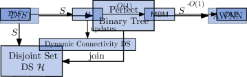
We focus on general disk graphs, with no assumption on the radius ratio. Our approach has two main ingredients. First, we simply represent the connected components in a data structure for the disjoint set union problem [1]. This allows for fast queries, in amortized time, also mentioned by Reif [5]. The second ingredient is an efficient data structure to find all components in that are intersected by any given disk (and hence tells us which components need to be merged after an insertion of a new site). A schematic overview of the data structure is given in Figure 1.
2 Insertion-Only Data Structure for Unbounded Radii
As in the incremental data structure for disk graphs with bounded radius ratio by Kaplan et al. [2], we use a disjoint set union data structure to represent the connected components of and to perform the connectivity queries. To insert a new site into , we first find the set of components in that are intersected by . Then, once is known, we can simply update the disjoint set union structure to support further queries.

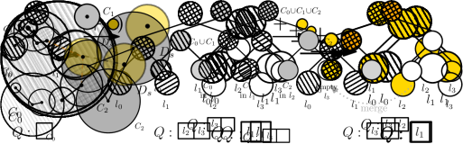
In order to identify efficiently, we use a component tree . This is a binary tree whose leaves store the connected components of . The idea is illustrated in Figure 2 showing a disk graph and its associated component tree. We require that is a complete binary tree, and some of its leaves may not have a connected component assigned to them, like in Figure 2. Those leaves are empty. Typically, we will not distinguish the leaf storing a connected component and the component itself. Also when suitable, we will treat a connected component as a set of sites. Every node of stores a fully dynamic additively weighted nearest neighbor data structure (AWNN). An AWNN stores a set of points, each associated with a weight . On a nearest neighbor query with a point it returns the point that minimizes . For this data structure, we use the following result by Kaplan et al. [3] with an improvement by Liu [4].
Lemma 2.1 (Kaplan et al. [3, Theorem 8.3, Section 9], Liu [4, Corollary 4.3]).
There is a fully dynamic AWNN data structure that allows insertions in amortized expected time and deletions in amortized expected time. Furthermore, a nearest neighbor query takes worst case time. The data structure requires space.
The component tree maintains the following invariants. Invariant 2 allows us to use a query to the AWNN to find the disk whose boundary is closed to a query point.
- Invariant 1:
-
Every connected component of is stored in exactly one leaf of , and
- Invariant 2:
-
The AWNN of a node contains the sites of all connected components that lie in the subtree rooted at , where a site has assigned weight .
In addition to , we store a queue that contains exactly the empty leaves in .
We now describe how to update when a new site is inserted. We maintain in such a way that the structure of changes only when creates a new isolated component in . In the following lemma, we consider the slightly more general case of inserting a new connected component that does not intersect any connected component already stored in .
Lemma 2.2.
Let be a component tree of height with sites and let be an isolated connected component. We can insert into in amortized time .
Proof 2.3.
The insertion performs two basic steps: first, we find or create an empty leaf into which can be inserted. Second, the AWNN structures along the path from to the root of are updated.
For the first step, we check if is non-empty. If so, we extract the first element from to obtain our empty leaf . If is empty, there are no empty leaves, and we have to expand the component tree. For this, we create a new root for , and we attach the old tree as one child. The other child is an empty complete tree of the same size as the old tree. This creates a complete binary tree, see intemediate state in Figure 3. We copy the AWNN of the former root to the new root, we add all new empty leaves to , and we extract from .

For the second step, we insert into , and we store an AWNN structure with the sites from in . Then, the AWNN structures on all ancestors of are updated by inserting the sites of , see Figure 4 and Figure 3 in case of tree extension respectively.

This procedure maintains both invariants: since an isolated component does not affect the remaining connected components of , it has to be inserted into a new leaf, maintaining the first invariant. The second invariant is taken care of in the second step, by construction. Afterwards, the queue has the correct state, since we extract the leaf used in the insertion.
The running time for finding or creating an empty leaf is amortized . This is immediate if , and otherwise, we can charge the cost of building the empty tree, inserting the empty leaves into , and producing an AWNN structure for the new root to the previous insertions. The most expensive step consists in updating the AWNN structures for the new component. In each of the AWNN structures of the ancestors of , we must insert disks. By 2.1, this results into an expected amortized time of .
Next, we describe how to find the set of connected components that are intersected by a disk .
Lemma 2.4.
Let be a component tree of height that stores disks. We can find in worst case time .
Proof 2.5.
First, observe that if the site returned by a query to an AWNN structure with does not intersect , then does not intersect any disk for the sites stored in this AWNN. Thus, the case where can be identified by a query to the AWNN structure in the root of , in time.
In any other case, we perform a top down traversal of . Let be the current node. We query the AWNN structures of both children of with , and we recurse only into the children where the nearest neighbor intersects . The set then contains exactly the connected components of all leaves where intersects its weighted nearest neighbor. Since every leaf found corresponds to one connected component intersecting and we recurse into all subtrees whose union of sites have a non-empty intersection with , we do not miss any connected components.
For every connected component, there are at most queries to AWNN structures along the path from the root to the components. A query takes amortized time by 2.1, giving an amortized time of , if is not isolated. The overall time follows from taking the maximum of both cases.
Lemma 2.6.
Let be a component tree that stores sites. A new site can be inserted into in amortized expected time.
Proof 2.7.
First, we use the algorithm from 2.4. to find . If , we use 2.2 to insert as a singleton isolated connected component.
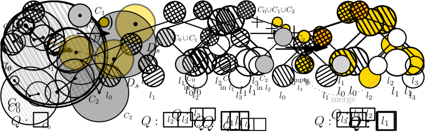
Otherwise, if , let be a largest connected component in . We insert into and into the AWNN structures of all ancestors of . Then, if , we are done, see Figure 5. If , all components in now form a new, larger, component in . We perform the following clean-up step in .
For each component , all sites from are inserted into . Let lca be the lowest common ancestor of the leaves for and in . Then all sites from are deleted from the AWNN structures along the path from to lca, and reinserted along the path from to lca. Finally, all newly empty leaves are inserted into . For an illustration of the insertion of and the clean-up step, see Figure 6.
To show correctness, we again argue that the invariants are maintained. If this follows by 2.2. In the other case, we directly insert into a connected component intersected by and update all AWNN structures along the way. As 2.4 correctly finds all relevant connected components, and we explicitly move the sites in these components to during clean-up, Invariant 1 is fulfilled. In a similar vein, we update all AWNN structures of sites that move to a new connected component, satisfying Invariant 2. Moreover, we keep updated by inserting or removing empty leaves when needed during the algorithm.
To complete the proof, it remains to analyze the running time. In the worst case, where all components are singletons, a component tree that stores sites has height . If the running time for finding is by 2.4. The insertion and restructuring is done with 2.2, yielding an expected amortized time of . In the case , with a running time of for finding follows by 2.4. Following similar arguments to the case , the time needed for the insertion and restructuring is expected amortized .
Finally, we consider the case . By 2.4, finding takes worst case time . Then the insertion of can be done in expected amortized time , as in the cases above. It remains to analyze the running time of the clean-up step. We know that the first common ancestor might be the root of . Hence, in the worst case, we have to perform insertions and deletions for a single clean-up step. As the time for the deletions in the AWNN structures dominates, this is expected amortized worst case time. Note that since and we have to insert , the running time of 2.4 is dominated by the clean-up step.
The overall time spent on all clean-up steps over all insertions is then upper bounded by . Observe, that during the lifetime of the component tree, each disk can only be merged into connected components. Thus, we have
and the overall expected time spent on clean-up steps is . As the case turned out to be the most complex case, the overall running time follows.
Theorem 2.8.
There is an incremental data structure for connectivity queries in disk graphs with amortized query time and expected amortized update time.
Proof 2.9.
We use a component tree as described above to maintain the connected components. Additionally, we maintain a disjoint set data structure , where each connected component forms a set, see Figure 1. Queries are performed directly in in amortized time.
When inserting an isolated component during the update, this component is added to . When merging several connected components in the clean-up step, this change is reflected in by suitable union operations. The time for updates in the component tree dominates the updates in , leading to an expected amortized update time of .
3 Conclusion
We introduced a data structure that solves the incremental connectivity problem in general disk graphs with amortized query and amortized expected update time. The question of finding efficient fully-dynamic data structures for both the general and the bounded case remains open.
References
- [1] Thomas H. Cormen, Charles E. Leiserson, Ronald L. Rivest, and Clifford Stein. Introduction to Algorithms, Third Edition. The MIT Press, 3rd edition, 2009.
- [2] Haim Kaplan, Alexander Kauer, Katharina Klost, Kristin Knorr, Wolfgang Mulzer, Liam Roditty, and Paul Seiferth. Dynamic connectivity in disk graphs. In 38th International Symposium on Computational Geometry (SoCG 2022), pages 49:1–49:17, 2022. doi:10.4230/LIPIcs.SoCG.2022.49.
- [3] Haim Kaplan, Wolfgang Mulzer, Liam Roditty, Paul Seiferth, and Micha Sharir. Dynamic planar Voronoi diagrams for general distance functions and their algorithmic applications. Discrete Comput. Geom., 64(3):838–904, 2020. doi:10.1007/s00454-020-00243-7.
- [4] Chih-Hung Liu. Nearly optimal planar nearest neighbors queries under general distance functions. SIAM Journal on Computing, 51(3):723–765, 2022. doi:10.1137/20m1388371.
- [5] John H. Reif. A topological approach to dynamic graph connectivity. Information Processing Letters, 25(1):65–70, 1987. doi:10.1016/0020-0190(87)90095-0.