Homological Neural Networks
A Sparse Architecture for Multivariate Complexity

Abstract

The rapid progress of Artificial Intelligence research came with the development of increasingly complex deep learning models, leading to growing challenges in terms of computational complexity, energy efficiency and interpretability. In this study, we apply advanced network-based information filtering techniques to design a novel deep neural network unit characterized by a sparse higher-order graphical architecture built over the homological structure of underlying data. We demonstrate its effectiveness in two application domains which are traditionally challenging for deep learning: tabular data and time series regression problems. Results demonstrate the advantages of this novel design which can tie or overcome the results of state-of-the-art machine learning and deep learning models using only a fraction of parameters. The code and the data are available at https://github.com/FinancialComputingUCL/HNN.

1 Introduction

Computational processes can be viewed as mapping operations from points or regions in space into points or regions in another space with different dimensionality and properties. Neural networks process information through stacked layers with different dimensions to efficiently represent the inherent structure of the underlying data. Uncovering this structure is however challenging since it is typically an unknown priori. Nevertheless, studying dependencies among variables in a dataset makes it possible to characterise the structural properties of the data and shape ad-hoc deep learning architectures on it. Specifically, the basic operation in deep neural networks consists of aggregating input signals into one output. This operation is most effective in scenarios where the spatial organization of the variables is a good proxy for dependency. However, in several real-world complex systems, modelling dependency structures requires the usage of a complex network representation. Graph Neural Networks have been introduced as one possible way to address this issue (Samek et al., 2021). However, they present two main limits: (i) they are designed for data defined on nodes of a graph (Yang et al., 2022), and (ii) they usually only explicitly consider low-order interactions as geometric priors (edges connecting two nodes), ignoring higher-order relations (triangles, tetrahedra, $\dots$). Instead, dependency is not simply a bi-variate relation between couples of variables and involves groups of variables with complex aggregation laws.

In this work, we propose a novel deep learning architecture that keeps into account higher-order interactions in the dependency structure as topological priors. Higher-order graphs are networks that connect not only vertices with edges (i.e. low-order 1-dimensional simplexes) but also higher-order simplexes (Torres & Bianconi, 2020). Indeed, any higher-order component can be described as a combination of lower-order components (i.e. edges connecting two vertices, triangles connecting three edges, $\dots$). The study of networks in terms of the relationship between structures at different dimensionality is a form of homology. In this work, we propose a novel multi-layer deep learning unit capable of fully representing the homological structure of data and we name it Homological Neural Network (HNN). This is a feed-forward unit where the first layer represents the vertices, the second the edges, the third the triangles, and so on. Each layer connects with the next homological level accordingly to the network’s topology representing dependency structures of the underlying input dataset. Information only flows between connected structures at different order levels, and homological computations are thus obtained. Neurons in each layer have a residual connection to a post-processing readout unit. HNN’s weights are updated through backward propagation using a standard gradient descent approach. Given the higher-order representation of the dependency structure in the data, this unit should provide better computational performances than those of fully connected multi-layer architectures. Furthermore, given the network representation’s intrinsic sparsity, this unit should be computationally more efficient, and results should be more intuitive to interpret. We test these hypotheses by evaluating the HNN unit on two application domains traditionally challenging for deep learning models: tabular data and time series regression problems.

This work builds upon a vast literature concerning complex network representation of data dependency structures (Costa-Santos et al., 2011; Moyano, 2017). Networks are excellent tools for representing complex systems both mathematically and visually, they can be used for both qualitatively describing the system and quantitatively modeling the system properties. A dense graph with everything connected with everything else (complete graph) does not carry any information, conversely, too sparse representations are oversimplifications of the important relations. There is a growing recognition that, in most practical cases, a good representation is provided by structures that are locally dense and globally sparse. In this paper we use a family of network representations, named Information Filtering Networks (IFNs), that have been proven to be particularly useful in data-driven modeling (Tumminello et al., 2005; Barfuss et al., 2016; Briola & Aste, 2023). The proposed methodology exploits the power of a specific class of IFNs, namely the Triangulated Maximally Filtered Graph (TMFG), which is a maximally planar chordal graph with a clique-three structure made of tetrahedra (Massara et al., 2017). The TMFG is a good compromise between sparsity and density and it is computationally efficient to construct. It has the further advantage of being chordal (every cycle of four or more vertices has a chord) which makes it possible to directly implement probabilistic graphical modeling on its structure (Barfuss et al., 2016).

The rest of the paper is organised as follows. We first review, in Section 2, the relevant literature. Then, in Section 3, we introduce a novel representation for higher-order networks, the founding stone of HNNs. The design of HNN as a modular unit of a deep learning architecture is discussed in Section 4. Application of HNN-based architectures to tabular data experiment on Penn Machine Learning Benchmark and to multivariate time-series on solar-energy power and exchange-rates datasets are discussed in Section 5.1 and Section 5.2. Conclusions are provided in Section 6.

2 Background literature

2.1 Information Filtering Networks

The construction of sparse network representations of complex datasets has been a very active research domain during the last two decades. There are various methodologies and possibilities to associate data with network representations. The overall idea is that in a complex dataset, each variable is represented by a vertex in the network, and the interaction between variables is associated with the network structure. Normally such a network representation is constructed from correlations or (non-linear) dependency measures (i.e. mutual information) and the network is constructed in such a way as to retain the largest significant dependency in its interconnection structure. These networks are known as Information Filtering Networks (IFN) with one of the best-known examples being the Minimum Spanning Tree (MST) (Nešetřil et al., 2001) built from pure correlations (Mantegna, 1998). The MST has the advantage of being the sparsest connected network and of being the exact solution for some optimization problems (Kruskal, 1956; Prim, 1957). However, other IFNs based on richer topological embeddings, such as planar graphs (Tumminello et al., 2005; Aste & Matteo, 2017) or clique trees and forests (Massara et al., 2017; Massara & Aste, 2019), can extract more valuable information and better represent the complexity of the data. These network constructions have been employed across diverse research domains from finance (Barfuss et al., 2016) to brain studies (Telesford et al., 2011), and psychology (Christensen et al., 2016). In this paper, we use the Triangulated Maximally Filtered Graph (TMFG) (Massara et al., 2017), which is a planar and chordal IFN. It has the property of being computationally efficient and it can yield a sparse precision matrix with the structure of the network, thereby being a tool for $L_{0}$-norm topological regularization in multivariate probabilistic models (Aste, 2022).

2.2 Sparse neural networks

Recent advances in artificial intelligence have exacerbated the challenges related to models’ computational and energy efficiency. To mitigate these issues, researchers have proposed new architectures characterized by fewer parameters and sparse structures. Some of them have successfully reduced the complexity of very large models to drastically improve efficiency with negligible performance degradation (Ye et al., 2018; Molchanov et al., 2016; Lee et al., 2018; Yu et al., 2017; Anwar et al., 2015; Molchanov et al., 2017; Zhuo et al., 2018; Wang et al., 2018). Others have not only simplified the architectures but also enhanced models’ efficacy, further demonstrating that fewer parameters yield better model generalization (Wu et al., 2020; Wen et al., 2016; Liu et al., 2015, 2017; Hu et al., 2016; Zhuang et al., 2018; Peng et al., 2019; Louizos et al., 2017).

Nonetheless, in the majority of literature, sparse topological connectivity is pursued either after the training phase, which bears benefits only during the inference phase, or during the back-propagation phase which usually adds complexity and run-time to the training. A very first attempt to solve these issues is represented by network-inspired pruning methods incorporated pruning at the earliest stage of the building process, allowing for the establishment of a foundational topological architecture that can then be elaborated upon (Stanley & Miikkulainen, 2002; Hausknecht et al., 2014; Mocanu et al., 2017). However, the most interesting solution is represented by Simplicial NNs (Ebli et al., 2020) and Simplicial CNNs (Yang et al., 2022). Indeed, these architectures constitute the very first attempt to exploit the topological properties of sparse graph representations to capture higher-order data relationships. Despite their novelty, the design of these neural network architectures limits them to pre-designed network data, without the possibility to easily scale to more general data types (e.g., tabular data and time series).

In this paper, we incorporate topological constraints within the design phase of the network architecture, generating a more intricate sparse topology derived from IFNs (Briola et al., 2022; Briola & Aste, 2022, 2023; Vidal-Tomas et al., 2023).

2.3 Deep Learning models for tabular data

Throughout the previous ten years, conventional machine learning algorithms, exemplified by gradient-boosted decision trees (GBDT) (Chen & Guestrin, 2016), have predominantly governed the landscape of tabular data modelling, exhibiting superior efficacy compared to deep learning methodologies. Although the encouraging results presented in the literature (Shwartz-Ziv et al., 2018; Poggio et al., 2020; Piran et al., 2020), deep learning tends to encounter significant hurdles when implemented on tabular data. The works of (Arik & Pfister, 2019) and (Hollmann et al., 2022) claim to achieve comparable results to tree models, but they are all very large attention/transformer-based models. Indeed, tabular data manifest a range of peculiar issues such as non-locality, data sparsity, heterogeneity in feature types, and an absence of a priori knowledge about underlying dependency structures. Therefore, tree ensemble methodologies, such as XGBoost, are still deemed as the optimal choice for tackling real-world tabular data related tasks (Friedman, 2001; Prokhorenkova et al., 2018; Grinsztajn et al., 2022). In this work, we propose a much more efficient sparse deep-learning model with similar results.

2.4 Deep Learning models for multivariate time-series

Existing research in multivariate time series forecasting can be broadly divided into two primary categories: statistical methods and deep learning-based methods. Statistical approaches usually assume linear correlations among variables (i.e., time series) and use their lagged dependency to forecast through a regression, as exemplified by the vector auto-regressive model (VAR) (Zivot & Wang, 2003) and Gaussian process model (GP) (Roberts et al., 2012). In contrast, deep learning-based methods, such as LSTNet (Lai et al., 2017) and TPA-LSTM (Shih et al., 2018), utilize Convolutional Neural Networks (CNN) to identify spatial dependencies among variables and combine them with Long Short-Term Memory (LSTM) networks to process the temporal information. Despite they have been widely applied across various application domains, including finance (Lu et al., 2020) and weather data (Wan et al., 2019), these architectures do not explicitly model dependency structures among variables, being strongly limited on the interpretability side.

Recently, spatio-temporal graph neural networks (STGNNs) (Shao et al., 2022a, b) have attracted interest reaching state-of-the-art performances, as exemplified by MTGNN (Wu et al., 2020). STGNNs integrate graph convolutional networks and sequential recurrent models, with the former addressing non-Euclidean dependencies among variables and the latter capturing temporal patterns. The inclusion of advanced convolutional or aggregational layers accounting for sparsity and higher-order interactions has resulted in further improvements of STGNNs (Wang & Aste, 2022; Calandriello et al., 2018; Chakeri et al., 2016; Rong et al., 2020; Hasanzadeh et al., 2020; Zheng et al., 2020; Luo et al., 2021; Kim & Oh, 2021). In this paper, we use the HNN unit as an advanced aggregational module to extract the dependency structure of variables from the temporal signals generated from LSTMs.

3 A novel representation for higher order networks and its use for HNN construction

The representation of undirected graphs explicitly accounts for the vertices and their connections through edges and, instead, does not explicitly account for other, higher-order, structures such as triangles, tetrahedra, and, in general, $d$-dimensional simplexes. Indeed, usually, an undirected graph is represented as a pair of sets, $\mathcal{G}=(V,E)$: the vertex set $V=(v_{1},...,v_{p})$ and the edge set $E$ which is made of pairs of edges $(v_{i},v_{j})$. The associated graphical representation is a network where vertices, represented as points, are connected through edges, represented as segments. This encoding of the structure accounts only for the edges skeleton of the network. However, in many real-world scenarios, higher-order sub-structures are crucial for the functional properties of the network and it is therefore convenient – and sometimes essential – to use a representation that accounts for them explicitly.

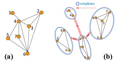
Figure 1: (a) Visual example of a higher order network made of 7 vertices, 11 edges, 6 triangles, and 1 tetrahedron. (b) This higher-order network is a clique tree made of four cliques (maximal cliques highlighted in the circles) connected through three separators (the tick red edges). One can observe that the separator constituted by the vertex ‘4’ has multiplicity 1, while the separator constituted of the edge ’4-6’ has multiplicity 2 and indeed it appears twice.

A simple higher-order representation can be obtained by adding triplets (triangles), quadruplets (tetrahedra), etc. to the sets in $\mathcal{G}$. However, the associated higher-order network is hard to handle both visually and computationally. In this paper, we propose an alternative approach, which consists of a layered representation that explicitly takes into account the higher order sub-structures and their interconnections. Such a representation is very simple, highly intuitive, of practical applicability as computational architecture, and, to the best of our knowledge, it has never been proposed before.

The proposed methodology is entirely based on a special class of networks: chordal graphs. These networks are constituted only of cliques organized in a higher order tree-like structure (also referred to as ‘clique tree’). This class of networks is very broad and it has many useful applications, in particular for probabilistic modeling (Aste, 2022). A visual example of a higher-order chordal network (a clique-tree), with 7 vertices, 11 edges, 6 triangles, and 1 tetrahedron, is provided in Figure 1. In the figure, the maximal cliques (largest fully-connected subgraphs) are highlighted and reported, in the right panel, as clique-tree nodes. Such nodes are connected to each other with links that are sub-cliques called separators. Separators have the property that, if removed from the network, they disconnect it into a number of components equal to the multiplicity of the separator minus one. In higher-order networks, cliques are the edge skeletons of simplexes. A 2-clique is a 1-dimensional simplex (an edge); 3-clique is a 2-dimensional simplex (a triangle); and so on with $(d+1)$-cliques being the skeleton of $d$-dimensional simplexes.

To represent the complexity of a higher-order network, we propose to adopt a layered structure (i.e. the Hasse diagram) where nodes in layer $d$ represent $d$-dimensional simplexes. The structures start with the vertices in layer 0; then a couple of vertices connect to edges represented in layer 1; edges connect to triangles in layer 2; triangles connect into tetrahedra in layer 3, and so on. This is illustrated in Figure 2. Such representation has a one-to-one correspondence with the original network but shows explicitly the simplexes and sub-simplexes and their interconnection in the structure. All information about the network at all dimensions is explicitly encoded in this representation including elements such as maximal cliques, separators, and their multiplicity (see caption of Figure 2).

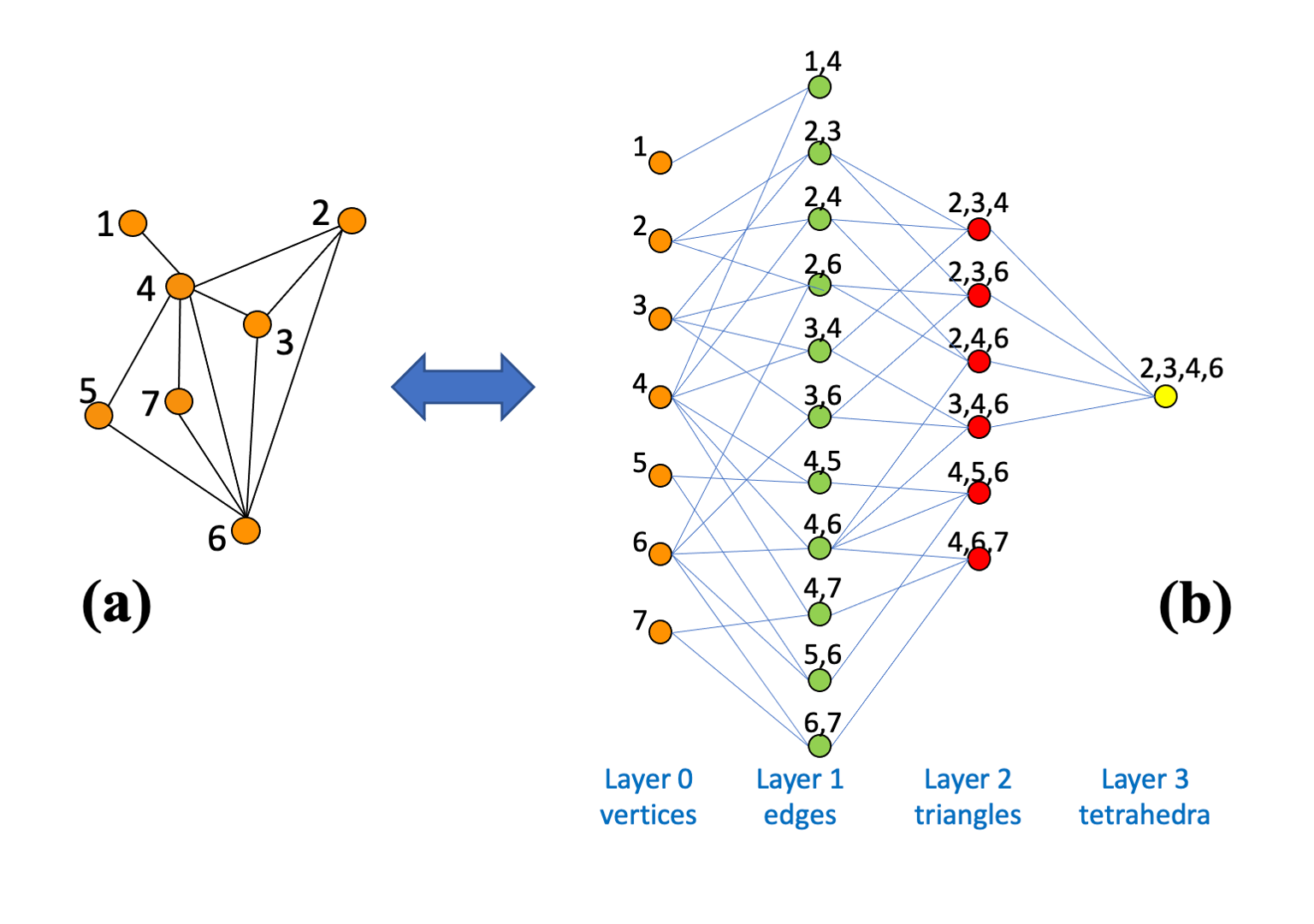
Figure 2: Higher order homological representation of the chordal graph in Figure 1 (reproduced in (a)). (b) Nodes in each layer, $L_{d}$, represent the $d$-dimensional simplexes in the structure. The links between nodes in layers $d$ and $d+1$ are the connections between $d$ to $d+1$ simplexes in the network. The degree on the left of nodes in $L_{d}$ is always equal to $d$. The degree on the right of nodes in $L_{d}$ can instead vary. The $d$-dimensional simplexes with no connections towards $d+1$ are the maximal cliques in the network (i.e. the nodes in the clique tree in Figure 1(b)).

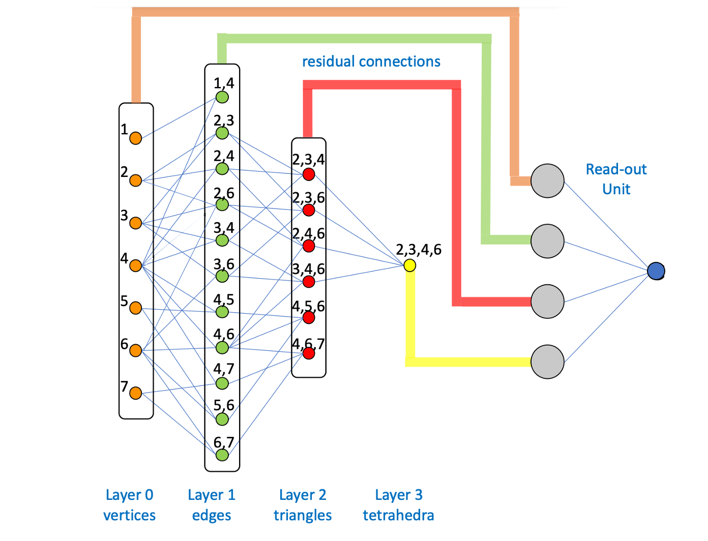
Figure 3: The Homological Neural Network (HNN) unit is constructed by using as input layer 0 of the homological representation of the dependency structure (see Figure 2(b)) and then feeding forward through the homological layers. The output is produced by a readout unit that connects all neurons in the layers. The HNN is essentially a sparse MLP unit with residual connections.

It is worth noting the resemblance of this layered structure with the layered architecture of deep neural networks. Indeed, we leverage this novel higher-order network representation as the neural network architecture of the HNN unit. In our experiments, the HNN is implemented from the TMFG generated from correlations. TMFG is computationally efficient, and can thus be used to dynamically re-configure the HNN according to changeable system conditions (Wang & Aste, 2022). The HNN architecture is illustrated in Figure 3. Essentially it is made by the layered representation of Figure 2 with the addition of the residual connections linking each neuron in each simplex layer to a final read-out layer. Such HNN is a sparse MLP-like neural network with extra residual connections and it can be employed as a modular unit. It can directly replace fully connected MLP layers in several neural network architectures. In this paper, the HNN unit is implemented using the standard PyTorch deep learning framework, while the sparse connection between layers is obtained thorugh the “sparselinear” PyTorch library.

4 Design of neural network architectures with HNN units for tabular data and time series studies

We investigate the performances of HNN units in two traditionally challenging application domains for deep learning: tabular data and time series regression problems. To process tabular data, the HNN unit can be directly fed with the data and it can be constructed from correlations by using the TMFG. In this case, the HNN unit acts as a sparsified MLP. This architecture is schematically shown in Figure 4. Instead, in spatio-temporal neural networks, the temporal layers are responsible for handling temporal patterns of individual series, whereas the spatial component learns their dependency structures. Consequently, the temporal part is usually modeled through the usage of recurrent neural networks (e.g. RNNs, GRUs, LSTMs), while the spatial component employs convolutional layers (e.g. CNNs) or aggregation functions (e.g. MLPs, GNNs).

Figure 5 presents the spatio-temporal neural network architecture employed in our multivariate time series experiments. The architecture consists of an LSTM for the temporal encoding of each time series and a graph generation unit that takes into account the correlation between different time series. This unit models time series as nodes and pairwise correlations as edges by imposing the topological constraints typical of the TMFG: planarity and chordality. The HNN is built based on the resulting sparse TMFG and aggregates each of the encoded time series from the LSTM, generating the final output.

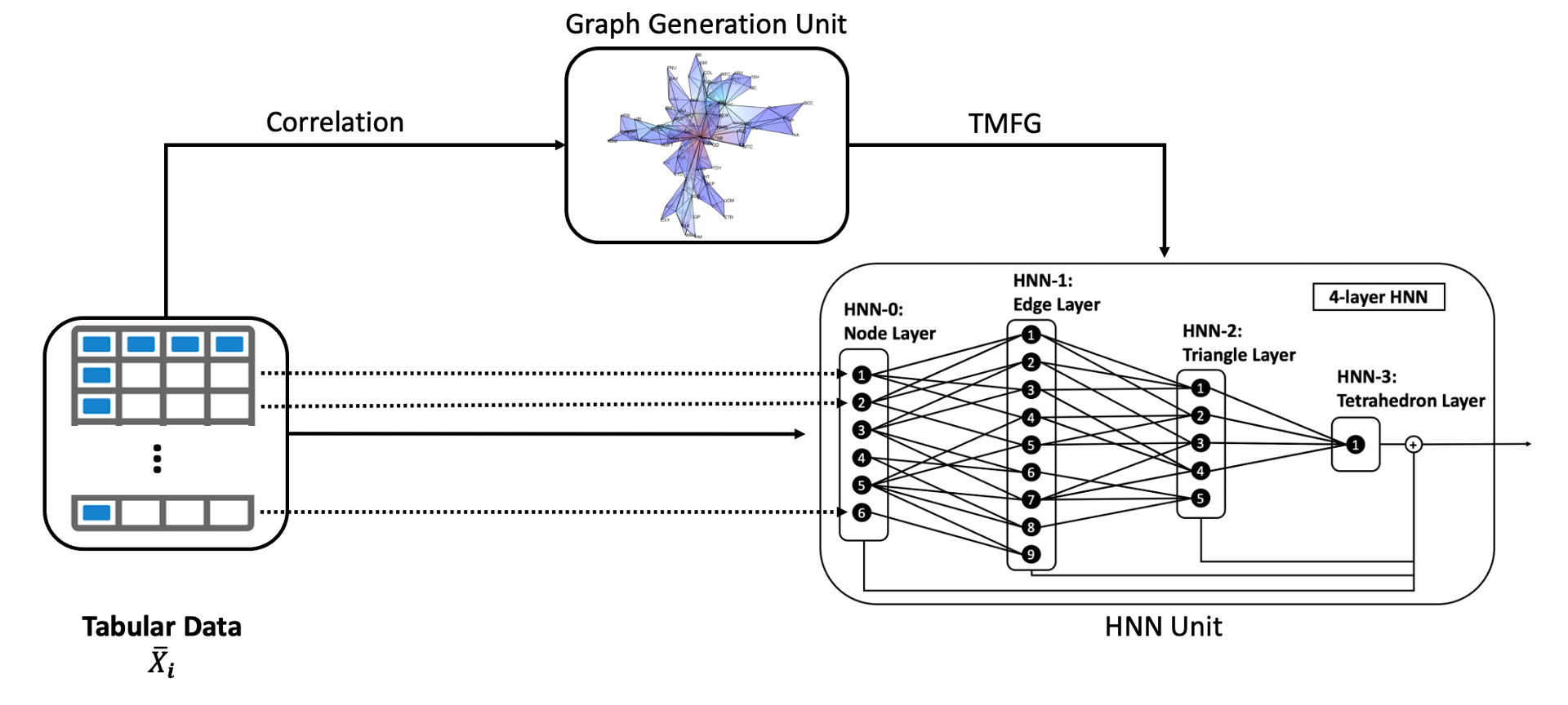
Figure 4: HNN architecture for tabular data. The tabular data is processed by a Graph Generation Unit to construct a prior sparse graph to represent spatial interdependencies between the feature columns. The prior graph guides the design of the HNN unit which then processes and transforms the feature columns into the final output.

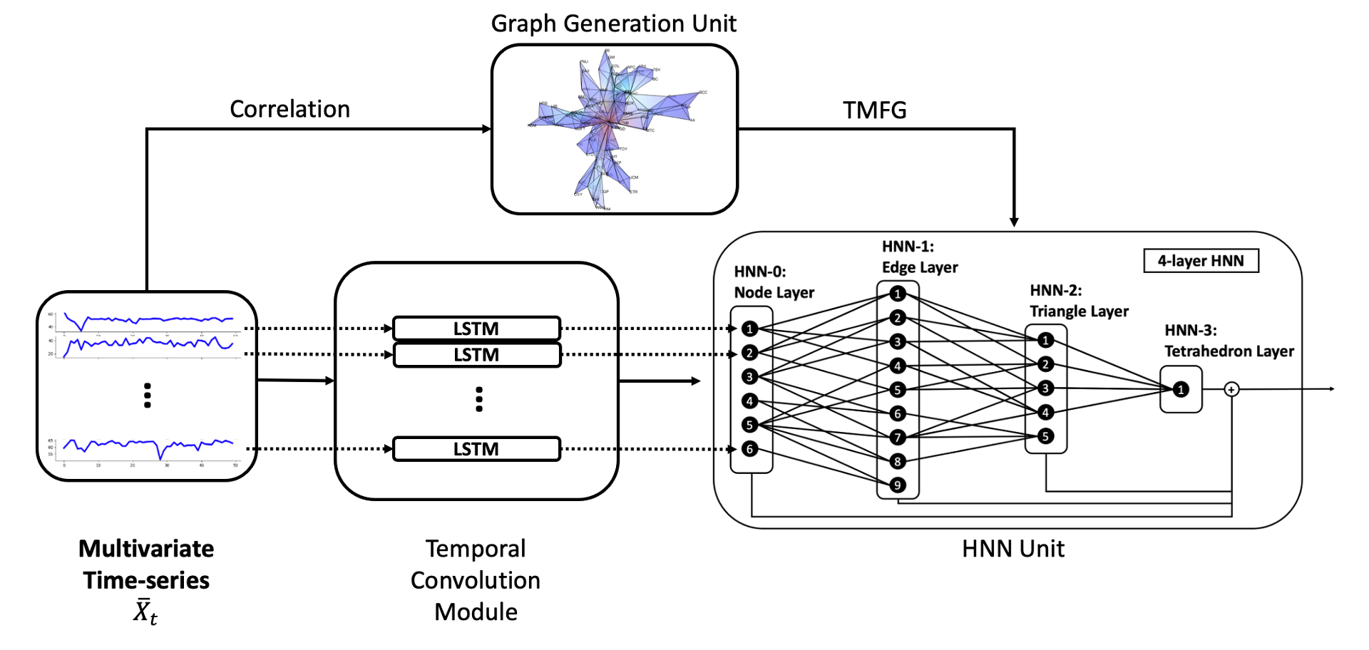
Figure 5: LSTM-HNN architecture for time-series data. The multivariate time-series is processed by a Graph Generation Unit to construct a prior sparse graph to represent spatial interdependencies, and each of the multivariate time series is processed separately by LSTM in the Temporal Convolution Module to harness the temporal information. The prior graph guides the design of the HNN unit which then aggregates the single temporal representations from LSTMs into the final output.

5 Results

5.1 Tabular Data

We test performances of the HNN architecture on the Penn Machine Learning Benchmark (PMLB) (Romano et al., 2021) regression dataset. We select datasets with more than 10,000 samples, and we split each of them into a 70% training and 30% testing set.

The R2 scores for the HNN architecture are reported in Table 1 for groups of PMLB regression datasets with different number of variables. We first compare HNN performances with the ones achieved by a Multi-Layer Perceptron (MLP) with same depth (i.e. 4 as imposed by the TMFG in the HNN’s building process). We also test a sparse MLP (MLP-HNN) with the same sparse structure of the HNN but without the residual connections from each layer to the final read-out layer, and a standard MLP with residual connections to the final read-out layer, MLP-res. All these architectures are optimized using gradient descent for the parameters and grid search for the hyper-parameters. It is evident from Table 1 that the HNN architecture largely outperforms the other neural network models. It is also evident that the homological structure of HNN is the main factor associated with improved performances (indeed MLP-HNN outperforms MLP) while the residual connections between layers are not the factor that makes HNN best performing (indeed MLP-res does not outperforms HNN).

	# variable $\in[0,20)$				# variable $\in[20,40)$				# variable $>40$
	mean	10th	50th	90th	mean	10th	50th	90th	mean	10th	50th	90th
HNN	${\bf 0.70}^{***}$	0.45	0.78	0.93	${\bf 0.75}^{**}$	0.55	0.78	0.91	${\bf 0.89}^{**}$	0.78	0.92	0.96
MLP-HNN	-9.64	-8.97	0.01	0.82	0.21	-0.01	0.03	0.56	0.55	0.14	0.54	0.96
MLP-res	-5.14	0.02	0.79	0.94	0.40	0.01	0.27	0.84	0.32	0.01	0.19	0.75
MLP	-7.18	-0.63	0.19	0.87	0.09	-0.01	-0.00	0.22	0.12	-0.14	-0.00	0.50

Table 1: R2 score from different models on PMLB regression dataset, with different number of variables. The best-performing average result is highlighted in bold, and ^∗ denotes $1\%$ significance, ^∗∗ for $0.1\%$ and ^∗∗∗ for $0.001\%$ respectively from paired T-test of the second best performing model result against HNN result. We also report the 10% 50% and 90% quantiles.

It is commonly acknowledged that neural network models do not perform well on tabular data (Borisov et al., 2021); tree-based models and the gradient boosting framework represent instead the state-of-the-art (Shwartz-Ziv & Armon, 2022; Grinsztajn et al., 2022). We therefore compare the HNN results with baseline models including Linear Regression (LM), Random Forest (RF), Light Gradient Boosting Machine (LGBM), Extreme Gradient Boosting Machine (XGB) (Ke et al., 2017; Chen & Guestrin, 2016). The experiments are performed on the same datasets using the optimization and tuning pipeline descirbed above.

	# variable $\in[0,20)$				# variable $\in[20,40)$				# variable $>40$
	mean	10th	50th	90th	mean	10th	50th	90th	mean	10th	50th	90th
HNN	0.70	0.45	0.78	0.93	0.75	0.55	0.78	0.91	0.89	0.78	0.92	0.96
XGB	${\bf 0.80}^{*}$	0.52	0.85	0.95	0.91	0.83	0.92	0.98	0.92	0.88	0.92	0.96
LGBM	0.65	0.00	0.81	0.95	0.89	0.81	0.91	0.97	0.91	0.87	0.91	0.95
RF	0.78	0.47	0.85	0.98	0.87	0.76	0.89	0.98	0.89	0.85	0.87	0.95
LM	0.53	0.12	0.64	0.90	0.36	0.01	0.28	0.74	0.34	0.11	0.25	0.65

Table 2: R2 score from different models on PMLB regression dataset, with a number of variables between 0 and 20, between 20 and 40, and larger than 40. The best-performing average result is highlighted in bold, and ^∗ denotes $1\%$ significance from paired T-test of the best-performing model result against HNN result. We also report the 10% 50% and 90% quantiles. The absence of ^∗ indicates statistical equivalence between the best-performing and HNN.

Table 2 and Figure 6 report the comparison between HNN results and the machine learning methods on the PMLB regression datasets. We underline that HNN outperforms traditional machine learning methods and nearly matches the state-of-the-art. Furthermore, the relative performance of HNN improves with the number of variables, notably with HNN obtaining equivalent and marginally better performance even than XGB for the datasets with large number of features (see Figure 6(d)).

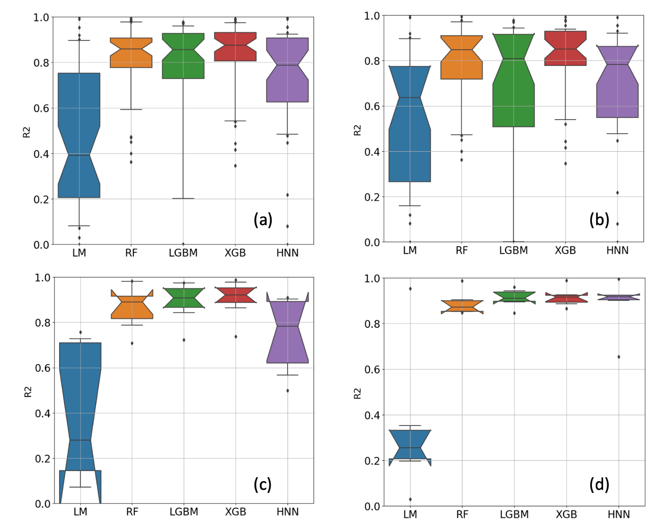
Figure 6: The R2 score from different models on PMLB (Penn Machine Learning Benchmarks) regression datasets. (a) All datasets (46 datasets). (b) Datasets with number of variable $\in[0,20)$ (32 datasets). (c) Datasets with number of variable $\in[20,40)$ (8 datasets). (d) Datasets with number of variable $\in[40,\inf)$ (6 datasets).

5.2 Multivariate Time-series Data

		solar-energy				exchange-rates
		Horizon (days)				Horizon (days)
Model	Metrics	3	6	12	24	3	6	12	24
LSTM-HNN	RSE	$\textbf{0.190}^{*}$	$\textbf{0.270}^{*}$	$\textbf{0.354}^{*}$	$\textbf{0.446}^{*}$	$\textbf{0.022}^{*}$	$\textbf{0.027}^{**}$	$\textbf{0.040}^{*}$	$\textbf{0.049}^{*}$
	CORR	0.981	$\textbf{0.964}^{*}$	$\textbf{0.942}^{*}$	$\textbf{0.902}^{**}$	$\textbf{0.976}^{***}$	$\textbf{0.968}^{**}$	$\textbf{0.956}^{*}$	$\textbf{0.938}^{*}$
LSTM-MLP-HNN	RSE	0.207	0.292	0.365	0.454	0.028	0.034	0.046	0.054
	CORR	0.980	0.959	0.936	0.893	0.965	0.957	0.945	0.928
LSTM-MLP-res	RSE	0.245	0.340	0.409	0.501	0.031	0.035	0.052	0.059
	CORR	0.972	0.944	0.905	0.898	0.850	0.829	0.835	0.828
LSTM-MLP	RSE	0.307	0.361	0.425	0.697	0.029	0.037	0.054	0.056
	CORR	0.956	0.937	0.898	0.723	0.845	0.838	0.834	0.824

Table 3: Relative Standard Error (RSE) and CORR (correlation). The best-performing results in a given metric and horizon are highlighted in bold. In addition, a paired T-test has been performed, and the p-values for the LSTM-HNN against the second-best-performing model (i.e. the LSTM-MLP-res) in the given metrics and horizon are highlighted next to the best-performing results, where ^∗ denotes $1\%$ significance, ^∗∗ for $0.1\%$ and ^∗∗∗ for $0.001\%$ respectively.

		solar-energy				exchange-rates
		Horizon (days)				Horizon (days)
Model	Metrics	3	6	12	24	3	6	12	24
LSTM-HNN	RSE	$0.190$	$0.270$	$0.354$	$0.446$	$0.022$	$0.027$	$0.040$	$0.049$
	CORR	$0.981$	$0.964$	$0.942$	$0.902$	$0.976$	$0.968$	$0.956$	0.938
MTGNN	RSE	$\textbf{0.177}^{*}$	$\textbf{0.234}^{**}$	$\textbf{0.310}^{*}$	$\textbf{0.427}^{*}$	0.019	0.025	0.034	0.045
	CORR	0.985	$\textbf{0.972}^{*}$	$\textbf{0.950}^{*}$	0.903	0.978	0.970	0.955	0.937
TPA-LSTM	RSE	0.180	0.234	0.323	0.438	$\textbf{0.017}^{*}$	0.024	0.034	0.044
	CORR	0.985	0.974	0.948	$\textbf{0.908}^{*}$	$\textbf{0.979}^{*}$	0.970	0.956	0.938
LSTNet-skip	RSE	0.184	0.255	0.325	0.464	0.022	0.028	0.035	0.044
	CORR	0.984	0.969	0.946	0.887	0.973	0.965	0.951	0.935
RNN-GRU	RSE	0.193	0.262	0.416	0.485	0.019	0.026	0.040	0.062
	CORR	0.982	0.967	0.915	0.882	0.978	0.971	0.953	0.922
GP	RSE	0.225	0.328	0.520	0.797	0.023	0.027	0.039	0.058
	CORR	0.975	0.944	0.851	0.597	0.871	0.819	0.848	0.827
VARMLP	RSE	0.192	0.267	0.424	0.684	0.026	0.039	0.040	0.057
	CORR	0.982	0.965	0.905	0.714	0.860	0.872	0.828	0.767
AR	RSE	0.243	0.379	0.591	0.869	0.022	0.027	0.035	0.044
	CORR	0.971	0.926	0.810	0.531	0.973	0.965	0.952	0.935

Table 4: Relative Standard Error and correlation. The best-performing results in a given metric and horizon are highlighted in bold. In addition, a paired T-test has been performed, and the p-values for the best-performing result against LSTM-HNN in the given metrics and horizon are highlighted next to the best-performing results, where ^∗ denotes $1\%$ significance, ^∗∗ for $0.1\%$ and ^∗∗∗ for $0.001\%$ respectively. The absence of ^∗ indicates statistical equivalence between the best-performing and LSTM-HNN models. When LSTM-HNN is the best-performing result, then the t-test is conversely performed against the second best-performing result.

The HNN module can be used as a portable component along with different types of neural networks to manage various input data structures and downstream tasks. In this Section, we apply HNN to process dependency structures in time series modelling after temporal dependencies are handled through the LSTM architecture. We use two different datasets which have been extensively investigated in the multivariate time-series literature (Wu et al., 2020): the solar-energy dataset from the National Renewable Energy Laboratory, which contains the solar-energy power output collected from 137 PV plants in Alabama State in 2007; and a financial dataset containing the daily exchange-rates rates of eight foreign countries including Australia, British, Canada, Switzerland, China, Japan, New Zealand, and Singapore in the period from 1990 to 2016 (see Table 5 in Appendix for further details).

Analogously with the tabular data, we first compare the outcomes of LSTM-HNN with those obtained with adapted MLP units. Specifically, LSTM units plus an MLP (LSTM-MLP); LSTM units plus an MLP with added residual connections to the final read-out layer (LSTM-MLP-res); and LSTM units plus a sparse MLP of the same layout as HNN without residual connections (LSTM-MLP-HNN). We then compare the LSTM-HNN results with traditional and state-of-the-art spatio-temporal models for multivariate time-series problems: auto-regressive model (AR) (Zivot & Wang, 2003); a hybrid model that exploits both the power of MLP and auto-regressive modelling (VARMLP) (Zhang, 2003); a Gaussian process (GP) (Roberts et al., 2012); a recurrent neural network with fully connected GRU hidden units (RNN-GRU) (Wu et al., 2020); a LSTM recurrent neural network combined with a convolutional neural network (LSTNet) (Lai et al., 2017); a LSTM recurrent neural network with attention mechanism (TPA-LSTM) (Shih et al., 2018); and a graph neural network with temporal and graph convolution (MTGNN) (Wu et al., 2020).

We evaluate performances of the LSTM-HNN and compare them with the ones achieved by benchmark methodologies by forecasting the solar-energy power outputs and the exchange-rates values at different time horizons with performances measured in terms of relative standard error (RSE) and correlation (CORR) (see Table 3). We underline that LSTM-HNN significantly outperforms all MLP-based models. On solar-energy data, LSTM-HNN reduces RSE by 38%, 25%, 17%, and 36% from LSTM-MLP and 8%, 7%, 3%, and 2% from LSTM-MLP-res across four horizons. On exchange-rates data, LSTM-HNN reduces RSE by 23%, 28%, 26%, and 13% from LSTM-MLP and 19%, 20%, 14%, and 10% from LSTM-MLP-res across four horizons.

We also notice that the residual connections from each layer to the final read-out layer are effective both in the HNN architecture (i.e. LSTM-HNN outperforms LSTM-MLP-HNN) and within the MPL models (i.e. LSTM-MLP-res outperforms LSTM-MLP). In order to illustrate the significance of the gain, a paired t-test of LSTM-HNN against LSTM-MLP-res has been performed revealing that all differences are significant at 1% or better with the only exception for the correlation at horizon 3 in the solar-energy output data.

The comparison between the results for LSTM-HNN and the other benchmark models is reported in Table 4. Results reveal that LSTM-HNN consistently outperforms all three non-RNN-based methods (AR, VARMLP and GP) on both datasets. It also outperforms LSTNet-skip results. LSTM-HNN outperforms RNN-GRU for all datasets and horizons except for the correlation in the exchange rates at horizon 6 where it returns an equivalent result accordingly with the paired t-test that was conducted between LSTM-HNN and the best-performing model. LSTM-HNN is instead slightly outperformed by MTGNN in most results for solar-power and by TPA-LSTM in several results for exchange-rates. It must be however noticed that these are massive deep-learning models with a much larger number of parameters (respectively 1.5 and 2.5 times larger than LSTM-HNN for the solar-energy datasets and 10 and 26 times larger for the exchange-rates datasets, see Table 6).

6 Conclusion

In this paper we introduce Homological Neural Networks (HNNs), a novel deep-learning architecture based on a higher-order network representation of multivariate data dependency structures. This architecture can be seen as a sparse MLP with extra residual connections and it can be applied in place of any fully-connected MLP unit in composite neural network models. We test the effectiveness of HNNs on tabular and time-series heterogeneous datasets. Results reveal that HNN, used either as a standalone model or as a modular unit within larger models, produces better results than MLP models with the same number of neurons and layers. We compare the performance of HNN with both fully-connected MLP, MLP sparsified with the HNN layered structure, and fully-connected MLP with additional residual connections and read-out unit. We design an experimental pipeline that verifies that the sparse higher-order homological layered structure on which HNN is built is the main element that eases the computational process. Indeed, we verify that the sparsified MLP with the HNN structure (MLP-HNN) over-performs all other MLP models. We also verify that the residual links between layers and the readout unit consistently improve HNN performances. Noticeably, although residual connections also improve fully-connected MLP performances, results are still inferior to the ones achieved by sparse MLP-HNN. We demonstrate that HNNs’ performances are in line with state-of-the-art best-performing computational models, however, it must be considered that they have a much smaller number of parameters, and their processing architecture is easier to interpret.

In this paper, we build HNNs from TMFG networks computed on pure correlations. TMFG are very convenient chordal network representations that are computationally inexpensive and provide opportunities for dynamically self-adjusting neural network structures. Future research work on HNN will focus on developing an end-to-end dynamic model that addresses the temporal evolution of variable interdependencies. TMFG is only one instance of a large class of chordal higher-order information filtering networks (Massara & Aste, 2019) which can be used as priors to construct HNN units. The exploration of this larger class of possible representations is a natural expansion of the present HNN configuration and will be pursued in future studies.

Appendix A Appendix

Dataset	No. Features	No. Samples	Sample Rate
solar-energy	137	52560	10 minutes
exchange-rates	8	7588	1 day

Table 5: Multivariate time-series dataset statistics, including the number of features, number of samples and sample rate in the solar-energy-energy and exchange-rates-rates datasets (Wu et al., 2020).

	solar-energy	exchange-rates
LSTM-MLP	452901	13011
LSTM-MLP-HNN	509208	13203
LSTM-MLP-res	509208	13203
LSTM-HNN	239061	12795

Table 6: Number of parameters in each model in solar-energy and exchange-rates datasets, comparing the sparse LSTM-HNN with the fully connected models.

	solar-energy	exchange-rates
LSTM-skip	337112	19478
TPA-LSTM	613987	132172
MTGNN	347665	337345
LSTM-HNN	239061	12795

Table 7: Number of parameters in each model in solar-energy and exchange-rates datasets, comparing the LSTM-HNN with respect to state-of-art models.

References

- Anwar et al. (2015) Anwar, S., Hwang, K., and Sung, W. Structured pruning of deep convolutional neural networks. ACM Journal on Emerging Technologies in Computing Systems (JETC), 13:1 – 18, 2015.
- Arik & Pfister (2019) Arik, S. Ö. and Pfister, T. Tabnet: Attentive interpretable tabular learning. ArXiv, abs/1908.07442, 2019.
- Aste (2022) Aste, T. Topological regularization with information filtering networks. Information Sciences, arXiv:2005.04692, 2022.
- Aste & Matteo (2017) Aste, T. and Matteo, T. Sparse causality network retrieval from short time series. Complex., 2017:4518429:1–4518429:13, 2017.
- Barfuss et al. (2016) Barfuss, W., Massara, G. P., Di Matteo, T., and Aste, T. Parsimonious modeling with information filtering networks. Physical Review E, 94(6), Dec 2016. ISSN 2470-0053. doi: 10.1103/physreve.94.062306. URL http://dx.doi.org/10.1103/PhysRevE.94.062306.
- Borisov et al. (2021) Borisov, V., Leemann, T., Sessler, K., Haug, J., Pawelczyk, M., and Kasneci, G. Deep neural networks and tabular data: A survey. IEEE transactions on neural networks and learning systems, PP, 2021.
- Briola & Aste (2022) Briola, A. and Aste, T. Dependency structures in cryptocurrency market from high to low frequency. 2022.
- Briola & Aste (2023) Briola, A. and Aste, T. Topological feature selection: A graph-based filter feature selection approach. ArXiv, abs/2302.09543, 2023.
- Briola et al. (2022) Briola, A., Vidal-Tom’as, D., Wang, Y., and Aste, T. Anatomy of a stablecoin’s failure: the terra-luna case. ArXiv, abs/2207.13914, 2022.
- Calandriello et al. (2018) Calandriello, D., Koutis, I., Lazaric, A., and Valko, M. Improved large-scale graph learning through ridge spectral sparsification. In ICML, 2018.
- Chakeri et al. (2016) Chakeri, A., Farhidzadeh, H., and Hall, L. O. Spectral sparsification in spectral clustering. 2016 23rd International Conference on Pattern Recognition (ICPR), pp. 2301–2306, 2016.
- Chen & Guestrin (2016) Chen, T. and Guestrin, C. Xgboost: A scalable tree boosting system. In Proceedings of the 22nd acm sigkdd international conference on knowledge discovery and data mining, pp. 785–794, 2016.
- Christensen et al. (2016) Christensen, D. L., Baio, J., Braun, K. V. N., Bilder, D. A., Charles, J. M., Constantino, J. N., Daniels, J. L., Durkin, M. S., Fitzgerald, R. T., Kurzius-Spencer, M., Lee, L. C., Pettygrove, S., Robinson, C. C., Schulz, E. G., Wells, C., Wingate, M. S., Zahorodny, W. M., and Yeargin-Allsopp, M. Prevalence and characteristics of autism spectrum disorder among children aged 8 years — autism and developmental disabilities monitoring network, 11 sites, united states, 2012. MMWR Surveillance Summaries, 65:1 – 23, 2016.
- Costa-Santos et al. (2011) Costa-Santos, C., Bernardes, J., Antunes, L. F. C., and de Campos, D. A. Complexity and categorical analysis may improve the interpretation of agreement studies using continuous variables. Journal of evaluation in clinical practice, 17 3:511–4, 2011.
- Ebli et al. (2020) Ebli, S., Defferrard, M., and Spreemann, G. Simplicial neural networks. arXiv preprint arXiv:2010.03633, 2020.
- Friedman (2001) Friedman, J. H. Greedy function approximation: a gradient boosting machine. Annals of statistics, pp. 1189–1232, 2001.
- Grinsztajn et al. (2022) Grinsztajn, L., Oyallon, E., and Varoquaux, G. Why do tree-based models still outperform deep learning on tabular data? ArXiv, abs/2207.08815, 2022.
- Hasanzadeh et al. (2020) Hasanzadeh, A., Hajiramezanali, E., Boluki, S., Zhou, M., Duffield, N. G., Narayanan, K. R., and Qian, X. Bayesian graph neural networks with adaptive connection sampling. ArXiv, abs/2006.04064, 2020.
- Hausknecht et al. (2014) Hausknecht, M. J., Lehman, J., Miikkulainen, R., and Stone, P. A neuroevolution approach to general atari game playing. IEEE Transactions on Computational Intelligence and AI in Games, 6:355–366, 2014.
- Hollmann et al. (2022) Hollmann, N., Muller, S., Eggensperger, K., and Hutter, F. Tabpfn: A transformer that solves small tabular classification problems in a second. 2022.
- Hu et al. (2016) Hu, H., Peng, R., Tai, Y.-W., and Tang, C.-K. Network trimming: A data-driven neuron pruning approach towards efficient deep architectures. ArXiv, abs/1607.03250, 2016.
- Ke et al. (2017) Ke, G., Meng, Q., Finley, T., Wang, T., Chen, W., Ma, W., Ye, Q., and Liu, T.-Y. Lightgbm: A highly efficient gradient boosting decision tree. In NIPS, 2017.
- Kim & Oh (2021) Kim, D. and Oh, A. H. How to find your friendly neighborhood: Graph attention design with self-supervision. In ICLR, 2021.
- Kruskal (1956) Kruskal, J. B. On the shortest spanning subtree of a graph and the traveling salesman problem. 1956.
- Lai et al. (2017) Lai, G., Chang, W.-C., Yang, Y., and Liu, H. Modeling long- and short-term temporal patterns with deep neural networks. The 41st International ACM SIGIR Conference on Research & Development in Information Retrieval, 2017.
- Lee et al. (2018) Lee, N., Ajanthan, T., and Torr, P. H. S. Snip: Single-shot network pruning based on connection sensitivity. ArXiv, abs/1810.02340, 2018.
- Liu et al. (2015) Liu, B., Wang, M., Foroosh, H., Tappen, M. F., and Pensky, M. Sparse convolutional neural networks. 2015 IEEE Conference on Computer Vision and Pattern Recognition (CVPR), pp. 806–814, 2015.
- Liu et al. (2017) Liu, Z., Li, J., Shen, Z., Huang, G., Yan, S., and Zhang, C. Learning efficient convolutional networks through network slimming. 2017 IEEE International Conference on Computer Vision (ICCV), pp. 2755–2763, 2017.
- Louizos et al. (2017) Louizos, C., Welling, M., and Kingma, D. P. Learning sparse neural networks through l0 regularization. ArXiv, abs/1712.01312, 2017.
- Lu et al. (2020) Lu, W., Li, J., Li, Y., Sun, A., and Wang, J. A cnn-lstm-based model to forecast stock prices. Complex., 2020:6622927:1–6622927:10, 2020.
- Luo et al. (2021) Luo, D., Cheng, W., Yu, W., Zong, B., Ni, J., Chen, H., and Zhang, X. Learning to drop: Robust graph neural network via topological denoising. Proceedings of the 14th ACM International Conference on Web Search and Data Mining, 2021.
- Mantegna (1998) Mantegna, R. N. Hierarchical structure in financial markets. The European Physical Journal B - Condensed Matter and Complex Systems, 11:193–197, 1998.
- Massara & Aste (2019) Massara, G. P. and Aste, T. Learning clique forests. ArXiv, abs/1905.02266, 2019.
- Massara et al. (2017) Massara, G. P., di Matteo, T., and Aste, T. Network filtering for big data: Triangulated maximally filtered graph. J. Complex Networks, 5:161–178, 2017.
- Mocanu et al. (2017) Mocanu, D. C., Mocanu, E., Stone, P., Nguyen, P. H., Gibescu, M., and Liotta, A. Scalable training of artificial neural networks with adaptive sparse connectivity inspired by network science. Nature Communications, 9, 2017.
- Molchanov et al. (2017) Molchanov, D., Ashukha, A., and Vetrov, D. P. Variational dropout sparsifies deep neural networks. ArXiv, abs/1701.05369, 2017.
- Molchanov et al. (2016) Molchanov, P., Tyree, S., Karras, T., Aila, T., and Kautz, J. Pruning convolutional neural networks for resource efficient transfer learning. ArXiv, abs/1611.06440, 2016.
- Moyano (2017) Moyano, L. G. Learning network representations. The European Physical Journal Special Topics, 226:499–518, 2017.
- Nešetřil et al. (2001) Nešetřil, J., Milková, E., and Nešetřilová, H. Otakar boruvka on minimum spanning tree problem translation of both the 1926 papers, comments, history. Discrete mathematics, 233(1-3):3–36, 2001.
- Peng et al. (2019) Peng, H., Wu, J., Chen, S., and Huang, J. Collaborative channel pruning for deep networks. In International Conference on Machine Learning, 2019.
- Piran et al. (2020) Piran, Z., Shwartz-Ziv, R., and Tishby, N. The dual information bottleneck. arXiv preprint arXiv:2006.04641, 2020.
- Poggio et al. (2020) Poggio, T., Banburski, A., and Liao, Q. Theoretical issues in deep networks. Proceedings of the National Academy of Sciences, 117(48):30039–30045, 2020.
- Prim (1957) Prim, R. C. Shortest connection networks and some generalizations. Bell System Technical Journal, 36:1389–1401, 1957.
- Prokhorenkova et al. (2018) Prokhorenkova, L., Gusev, G., Vorobev, A., Dorogush, A. V., and Gulin, A. Catboost: unbiased boosting with categorical features. Advances in neural information processing systems, 31, 2018.
- Roberts et al. (2012) Roberts, S. J., Osborne, M. A., Ebden, M., Reece, S., Gibson, N. P., and Aigrain, S. Gaussian processes for timeseries modelling. 2012.
- Romano et al. (2021) Romano, J. D., Le, T. T., La Cava, W., Gregg, J. T., Goldberg, D. J., Chakraborty, P., Ray, N. L., Himmelstein, D., Fu, W., and Moore, J. H. Pmlb v1.0: an open source dataset collection for benchmarking machine learning methods. arXiv preprint arXiv:2012.00058v2, 2021.
- Rong et al. (2020) Rong, Y., bing Huang, W., Xu, T., and Huang, J. Dropedge: Towards deep graph convolutional networks on node classification. In ICLR, 2020.
- Samek et al. (2021) Samek, W., Montavon, G., Lapuschkin, S., Anders, C. J., and Müller, K.-R. Explaining deep neural networks and beyond: A review of methods and applications. Proceedings of the IEEE, 109:247–278, 2021.
- Shao et al. (2022a) Shao, Z., Zhang, Z., Wang, F., and Xu, Y. Pre-training enhanced spatial-temporal graph neural network for multivariate time series forecasting. Proceedings of the 28th ACM SIGKDD Conference on Knowledge Discovery and Data Mining, 2022a.
- Shao et al. (2022b) Shao, Z., Zhang, Z., Wei, W., Wang, F., Xu, Y., Cao, X., and Jensen, C. S. Decoupled dynamic spatial-temporal graph neural network for traffic forecasting. ArXiv, abs/2206.09112, 2022b.
- Shih et al. (2018) Shih, S.-Y., Sun, F.-K., and yi Lee, H. Temporal pattern attention for multivariate time series forecasting. Machine Learning, pp. 1–21, 2018.
- Shwartz-Ziv & Armon (2022) Shwartz-Ziv, R. and Armon, A. Tabular data: Deep learning is not all you need. Inf. Fusion, 81:84–90, 2022.
- Shwartz-Ziv et al. (2018) Shwartz-Ziv, R., Painsky, A., and Tishby, N. Representation compression and generalization in deep neural networks, 2018.
- Stanley & Miikkulainen (2002) Stanley, K. O. and Miikkulainen, R. Evolving neural networks through augmenting topologies. Evolutionary Computation, 10:99–127, 2002.
- Telesford et al. (2011) Telesford, Q. K., Simpson, S., Burdette, J., Hayasaka, S., and Laurienti, P. The brain as a complex system: Using network science as a tool for understanding the brain. Brain connectivity, 1 (4):295–308, 2011.
- Torres & Bianconi (2020) Torres, J. J. and Bianconi, G. Simplicial complexes: higher-order spectral dimension and dynamics. Journal of Physics: Complexity, 1, 2020.
- Tumminello et al. (2005) Tumminello, M., Aste, T., Di Matteo, T., and Mantegna, R. N. A tool for filtering information in complex systems. Proceedings of the National Academy of Sciences, 102(30):10421–10426, 2005. ISSN 0027-8424. doi: 10.1073/pnas.0500298102. URL https://www.pnas.org/content/102/30/10421.
- Vidal-Tomas et al. (2023) Vidal-Tomas, D., Briola, A., and Aste, T. Ftx’s downfall and binance’s consolidation: The fragility of centralized digital finance. SSRN Electronic Journal, 2023.
- Wan et al. (2019) Wan, R., Mei, S., Wang, J., Liu, M., and Yang, F. Multivariate temporal convolutional network: A deep neural networks approach for multivariate time series forecasting. Electronics, 2019.
- Wang et al. (2018) Wang, D., Zhou, L., Zhang, X., Bai, X., and Zhou, J. Exploring linear relationship in feature map subspace for convnets compression. ArXiv, abs/1803.05729, 2018.
- Wang & Aste (2022) Wang, Y. and Aste, T. Network filtering of spatial-temporal gnn for multivariate time-series prediction. Proceedings of the Third ACM International Conference on AI in Finance, 2022.
- Wen et al. (2016) Wen, W., Wu, C., Wang, Y., Chen, Y., and Li, H. H. Learning structured sparsity in deep neural networks. ArXiv, abs/1608.03665, 2016.
- Wu et al. (2020) Wu, Z., Pan, S., Long, G., Jiang, J., Chang, X., and Zhang, C. Connecting the dots: Multivariate time series forecasting with graph neural networks. Proceedings of the 26th ACM SIGKDD International Conference on Knowledge Discovery & Data Mining, 2020.
- Yang et al. (2022) Yang, M., Isufi, E., and Leus, G. Simplicial convolutional neural networks. In ICASSP 2022-2022 IEEE International Conference on Acoustics, Speech and Signal Processing (ICASSP), pp. 8847–8851. IEEE, 2022.
- Ye et al. (2018) Ye, J., Lu, X., Lin, Z. L., and Wang, J. Z. Rethinking the smaller-norm-less-informative assumption in channel pruning of convolution layers. ArXiv, abs/1802.00124, 2018.
- Yu et al. (2017) Yu, R., Li, A., Chen, C.-F., Lai, J.-H., Morariu, V. I., Han, X., Gao, M., Lin, C.-Y., and Davis, L. S. Nisp: Pruning networks using neuron importance score propagation. 2018 IEEE/CVF Conference on Computer Vision and Pattern Recognition, pp. 9194–9203, 2017.
- Zhang (2003) Zhang, G. P. Time series forecasting using a hybrid arima and neural network model. Neurocomputing, 50:159–175, 2003.
- Zheng et al. (2020) Zheng, C., Fan, X., Wang, C., and Qi, J. Gman: A graph multi-attention network for traffic prediction. ArXiv, abs/1911.08415, 2020.
- Zhuang et al. (2018) Zhuang, Z., Tan, M., Zhuang, B., Liu, J., Guo, Y., Wu, Q., Huang, J., and Zhu, J.-H. Discrimination-aware channel pruning for deep neural networks. In Neural Information Processing Systems, 2018.
- Zhuo et al. (2018) Zhuo, H., Qian, X., Fu, Y., Yang, H., and Xue, X. Scsp: Spectral clustering filter pruning with soft self-adaption manners. ArXiv, abs/1806.05320, 2018.
- Zivot & Wang (2003) Zivot, E. and Wang, J. Vector autoregressive models for multivariate time series. 2003.