Unsupervised Episode Generation for Graph Meta-learning

Abstract.

We investigate Unsupervised Episode Generation methods to solve Few-Shot Node-Classification (FSNC) task via Meta-learning without labels. Dominant meta-learning methodologies for FSNC were developed under the existence of abundant labeled nodes from diverse base classes for training, which however may not be possible to obtain in the real-world. Although a few studies tried to tackle the label-scarcity problem in graph meta-learning, they still rely on a few labeled nodes, which hinders the full utilization of the information of all nodes in a graph. Despite the effectiveness of graph contrastive learning (GCL) methods in the FSNC task without using the label information, they mainly learn generic node embeddings without consideration of the downstream task to be solved, which may limit its performance in the FSNC task. To this end, we propose a simple yet effective unsupervised episode generation method to benefit from the generalization ability of meta-learning for the FSNC task, while resolving the label-scarcity problem. Our proposed method, called Neighbors as Queries (NaQ), generates training episodes based on pre-calculated node-node similarity. Moreover, NaQ is model-agnostic; hence, it can be used to train any existing supervised graph meta-learning methods in an unsupervised manner, while not sacrificing much of their performance or sometimes even improving them. Extensive experimental results demonstrate the potential of our unsupervised episode generation methods for graph meta-learning towards the FSNC task. Our code is available at: https://github.com/JhngJng/NaQ-PyTorch

1. Introduction

Graph-structured data are useful and widely applicable in the real-world, due to their capability of modeling complex relationships between objects such as user-user relationship in social networks and product networks, etc. To handle tasks such as node classification on graph-structured data, Graph Neural Networks (GNNs) are widely used and have shown remarkable performance (Welling and Kipf, 2017; Veličković et al., 2018). However, it is well known that GNNs suffer from poor generalization when only a small number of labeled samples are provided (Zhou et al., 2019; Ding et al., 2020; Wang et al., 2022).

To mitigate such issues inherent in the ordinary deep neural networks, few-shot learning methods have emerged, and the dominant paradigm is applying meta-learning algorithms such as MAML (Finn et al., 2017) and ProtoNet (Snell et al., 2017), which are based on the episodic learning framework suggested in (Vinyals et al., 2016). Recent studies have proposed graph meta-learning models (Zhou et al., 2019; Ding et al., 2020; Huang and Zitnik, 2020; Wang et al., 2022) aiming at solving the Few-Shot Node Classification (FSNC) task on graphs by also leveraging the episodic learning framework, which is the main focus of this work.

Despite their effectiveness, existing graph meta-learning models require abundant labeled samples from diverse base classes for training. As presented in Figure 1(b), such label scarcity leads to a severe performance drop in existing supervised graph meta-learning models (i.e., TENT (Wang et al., 2022), G-Meta (Huang and Zitnik, 2020), ProtoNet (Snell et al., 2017), and MAML (Finn et al., 2017)) in FSNC. However, gathering enough labeled data from diverse classes may not be possible, and is costly in reality. Moreover, as these methods depend on a few labeled nodes from base classes, they are also vulnerable to the noisy labels in the base classes (See Figure 1(a)) and they are unable to fully utilize the information of all nodes in the graph.

A few recent studies (Wang et al., 2023; Kim et al., 2023) aim to alleviate the label-scarcity problem in FSNC. Specifically, TEG (Kim et al., 2023) utilizes equivariant neural networks to capture task-patterns shared among training episodes regardless of node labels, enabling the learning of highly transferable task-adaptation strategies even with a limited number of base classes and labeled nodes. X-FNC (Wang et al., 2023) obtains pseudo-labeled nodes via label propagation based on Poisson Learning, and the model is optimized based on information bottleneck to discard irrelevant information within the augmented support set. Although these methods extract useful meta-knowledge based on training episodes (Kim et al., 2023) or from pseudo-labeled nodes (Wang et al., 2023), they still highly depend on a few labeled nodes during the model training, and thus still fall short of utilizing the information of all nodes in the graph. As a result, their FSNC performance degrades as the number of labeled nodes and the number of base classes decrease as shown empirically in (Wang et al., 2023; Kim et al., 2023). In this respect, unsupervised methods are indispensable to fundamentally address the label-dependence problem inherent in existing graph meta-learning methods.

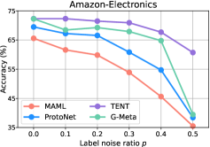
(a)

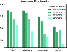
(b)

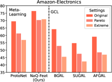
(c)

Figure 1. (a): Impact of the label noise $p$ (randomly injected) on 5-way 1-shot FSNC of the supervised graph meta-learning models. (b): Impact of the label-scarcity on 5-way 1-shot FSNC performance of the supervised graph meta-learning models. ‘Class%’ and ‘Label%’ denote the rate of available base classes during training and the rate of available labeled samples for each class, respectively. (c): Impact of the class imbalance on 5-way 1-shot FSNC performance. For the ‘Pareto’ setting, we kept the nodes for the top 20% classes, while keeping only 10 nodes for the remaining classes. For the ‘Extreme’ setting, the only difference from the ‘Pareto’ setting is that we kept nodes only for the top 5 classes instead of top 20% classes.

Most recently, TLP (Tan et al., [n. d.]) empirically demonstrated a simple linear probing with node embeddings that are pretrained by GCL methods, which are unsupervised, outperforms existing supervised graph meta-learning methods in FSNC. This is because GCL methods tend to generate generic node embeddings, since all nodes in a graph are involved in the training.

However, despite the effectiveness of generic node embeddings, we argue that they are vulnerable to inherent bias in the graph, which might lead to a significant performance drop depending on the downstream task. For example, if the given graph mainly consists of nodes from the majority classes (i.e., class imbalance), GCL methods have difficulty in learning embeddings of nodes from the minority classes, which results in poor FSNC performance on such minority classes. On the other hand, as each episode in the episodic learning framework reveals the ‘format’ of the FSNC task, meta-learning methods are rather more robust to the inherent bias that may exist in the given graph. To corroborate our argument, we modified the original graph to simulate two class imbalance settings (i.e., ‘Pareto’ and ‘Extreme’), and evaluated existing GCL methods (i.e., BGRL (Thakoor et al., 2022), SUGRL (Tan et al., [n. d.]), AFGRL (Lee et al., 2022b)) and meta-learning methods (i.e., ProtoNet (Snell et al., 2017) and NaQ-Feat (ours)) on the FSNC task (See Figure 1(c)). As expected, the performance of GCL methods deteriorated under class imbalance settings, while the performance drop of meta-learning methods was relatively moderate.

In summary, GCL methods are trained in an unsupervised manner by fully utilizing all nodes in a graph, and thus achieve satisfactory performance in general. On the other hand, meta-learning methods that adopt the episodic learning framework is aware of the downstream task, and thus particularly perform well on FSNC task under inherent bias in the graph. Hence, we argue that the FSNC performance can be further enhanced by achieving the best of both worlds of 1) GCL methods that fully utilize all nodes in a graph in an unsupervised manner, and 2) meta-learning methods whose episodic learning framework is aware of the downstream task (i.e., FSNC task).

In this work, we propose a simple yet effective unsupervised episode generation method named as Neighbors as Queries (NaQ) to benefit from the generalization ability of meta-learning methods for the FSNC task, while resolving the label-scarcity problem. The main idea is to construct a support set by randomly choosing nodes from the entire graph, and generate a corresponding query set via sampling similar nodes based on pre-calculated node-node similarity. It is important to note that our unsupervised episode generation method is model-agnostic, i.e., it can be used to train any existing supervised graph meta-learning methods in an unsupervised manner directly or only with minor modifications.

To sum up, our contributions are summarized as follows:

1. We present unsupervised episode generation method called NaQ, to solve FSNC problem via meta-learning without using label information during training. To our best knowledge, this is the first study that focuses on the episode generation to apply graph meta-learning in an unsupervised manner.

2. NaQ is model-agnostic; that is, it can be used to train any existing supervised graph meta-learning methods in an unsupervised manner, while not sacrificing much of their performance or sometimes even improving them, without using any labeled nodes.

3. Extensive experiments conducted on the four benchmark datasets demonstrate the effectiveness of NaQ. These results highlight the potential of the unsupervised graph meta-learning framework, which we propose for the first time in this work.

2. Preliminaries

2.1. Problem Statement

Let $\mathcal{G}=(\mathcal{V},\mathcal{E},X)$ be a graph, where $\mathcal{V},\ \mathcal{E}\subset\mathcal{V}\times\mathcal{V},\ X\in\mathbb{R}^{|\mathcal{V}|\times d}$ are a set of nodes, a set of edges, and a $d$-dimensional node feature matrix, respectively. We also use $X$ to denote a set of node features, i.e., $X=\{x_{v}:v\in\mathcal{V}\}$. Let $C$ be a set of total node classes. Here, we denote the base classes, a set of node classes that we can utilize during the training phase, as $C_{b}$, and denote the target classes, a set of node classes that we aim to recognize in downstream tasks with given a few labeled samples, as $C_{t}$. Note that $C_{b}\cup C_{t}=C$ and $C_{b}\cap C_{t}=\emptyset$. Usually, target classes $C_{t}$ are unknown during the training phase. In common few-shot learning settings, the number of labeled nodes from classes of $C_{b}$ is sufficient, while we only have a few labeled nodes from classes of $C_{t}$ in downstream tasks. Now we formulate the ordinary supervised FSNC problem as follows:

Definition 2.1 (Supervised few-shot node classification).

Given a graph $\mathcal{G}=(\mathcal{V},\mathcal{E},X)$ and labeled data $(X_{C_{b}},Y_{C_{b}})$, the goal of supervised few-shot node classification is to make predictions for $x_{q}\in X_{C_{t}}$ (i.e. query set) based on a few labeled samples $(x_{s},y_{s})\in(X_{C_{t}},Y_{C_{t}})$ (i.e. support set) with model $f_{\theta}$ trained on $(X_{C_{b}},Y_{C_{b}})$.

Based on this problem formulation, we can formulate the unsupervised FSNC problem as below. The only difference is that labeled nodes are not available during the model training.

Definition 2.2 (Unsupervised few-shot node classification).

Given a graph $\mathcal{G}=(\mathcal{V},\mathcal{E},X)$ and unlabeled data $X=X_{C_{b}}\cup X_{C_{t}}$, the goal of unsupervised few-shot node classification is to make predictions for $x_{q}\in X_{C_{t}}$ (i.e. query set) based on a few labeled samples $(x_{s},y_{s})\in(X_{C_{t}},Y_{C_{t}})$ (i.e. support set) with model $f_{\theta}$ trained on $X$.

Overall, the main goal of FSNC is to train a model $f_{\theta}$ on training data, and to adapt well to unseen target classes $C_{t}$ only using a few labeled samples. In this work, we study how to apply meta-learning algorithms in an unsupervised manner aiming at solving the FSNC task. More formally, our goal is to solve a $N$-way $K$-shot FSNC task (Vinyals et al., 2016), where $N$ is the number of distinct target classes and $K$ is the number of labeled samples in a support set. Moreover, there are $Q$ query samples given to be classified in each downstream task.

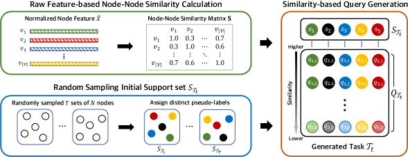
Figure 2. Overview of the NaQ. First, we calculate node-node similarity based on cosine similarity obtained from normalized raw node feature $\hat{X}$ before the training phase. Then, we generate a support set by randomly sampling $N$ nodes from the entire graph and giving distinct labels to them. Next, we find the $Q$ most similar nodes for each support set node. Finally, we generate task $\mathcal{T}_{t}$ by setting the sampled $N$ bundle of $Q$ nodes as the query set for each $N$ support set node.

2.2. Episodic Learning Framework

Our approach follows the episodic training framework (Vinyals et al., 2016) that is formally defined as follows:

Definition 2.3 (Episodic Learning).

Episodic learning is a learning framework that utilizes given bundle of tasks $\{\mathcal{T}_{t}\}_{t=1}^{T}$, where $\mathcal{T}_{t}=(S_{\mathcal{T}_{t}},\ Q_{\mathcal{T}_{t}})$, $S_{\mathcal{T}_{t}}=\{(x^{spt}_{t,i},y^{spt}_{t,i})\}_{i=1}^{N\times K}$ and $Q_{\mathcal{T}_{t}}=\{(x^{qry}_{t,i},y^{qry}_{t,i})\}_{i=1}^{N\times Q}$, instead of commonly used mini-batches in stochastic optimization.

By mimicking the ‘format’ of the downstream task (i.e., FSNC task), the episodic learning allows the model to be aware of the task to be solved in the testing phase. Current supervised meta-learning approaches require a sufficient amount of labeled samples in the training set $(X_{C_{b}},Y_{C_{b}})$ and a sufficient number of base classes $|C_{b}|$ (i.e., diverse base classes) to generate informative training episodes. However, gathering enough labeled data from diverse classes may not be possible and is usually costly in the real-world. As a result, supervised models fall short of utilizing the information of all nodes in the graph as they rely on a few labeled nodes, and thus lack generalizability. Hence, we propose unsupervised episode generation methods not only to benefit from the episodic learning framework that enables downstream task-aware learning of node embeddings, but also to resolve the label-scarcity problem and limited utilization of nodes in the training phase.

3. Methodology

3.1. Motivation

There are two essential components in the episodic learning framework, i.e., support set and query set. In each episode, the support set provides basic information about the task to be solved (analogous to contents in a textbook), while the query set enables the model to understand about how to solve the given task (analogous to exercises in the corresponding textbook). For this reason, the ‘exercises’ (query set) should share similar semantics as the ‘contents’ (support set) in the textbook. Motivated by the characteristic of episodic learning, we consider the similarity condition as the key to our proposed query generation process. Note that in the ordinary supervised setting, the similarity condition is easily achievable, since labels of the support set and query set are known, and thus can be sampled from the same class. However, as our goal is to generate training episodes in an unsupervised manner, how to sample a query set that is similar to each support set is non-trivial.

3.2. NaQ: Neighbors as Queries

In this work, we propose a simple yet effective query generation method, called Neighbors as Queries (NaQ), which leverages raw feature-level similar nodes as queries. The overview of NaQ can be found in Figure 2.

To generate $\{\mathcal{T}_{t}\}_{t=1}^{T}$, we start by randomly sampling $T$ sets of $N$ nodes from the entire graph, i.e., $\mathcal{T}_{t}=\{x_{t,i}\ |\ x_{t,i}\in\mathcal{V}\}_{i=1}^{N\times 1}$. Next, we assign pseudo-labels $y_{t,i}$ to each node $x_{t,i}\in\mathcal{T}_{t}$, i.e., $S_{\mathcal{T}_{t}}=\{(x_{t,i},y_{t,i})\ |\ x_{t,i}\in\mathcal{V}\}_{i=1}^{N\times 1}$, and consider the set of nodes as the support set. Then, we generate a corresponding query set $Q_{\mathcal{T}_{t}}$ with Top-Q similar nodes of each node $x_{t,i}$ in $S_{\mathcal{T}_{t}}$, and give them the same pseudo-label $y_{t,i}$.

To sample such ‘similar’ nodes to be used as queries, we utilize the cosine similarity between nodes calculated based on the raw node feature $X$ before the model training. Specifically, the node-node similarity matrix is calculated as $\mathbf{S}=\hat{X}\hat{X}^{T}$. Here, $\hat{X}$ denotes the row-normalized node feature matrix, where $\hat{x}_{v}=x_{v}/\|x_{v}\|_{2}$ for each node $v\in\mathcal{V}$. Since node features in our datasets are all words in documents (abstracts, product descriptions), we use the cosine similarity as a similarity measure (Tan et al., 2018). Other measures (e.g. Euclidean distance) can be considered for the other cases. Formally, we can express this query generation process as follows:

(1) $$\small Q_{\mathcal{T}_{t}}=\bigcup_{(x_{t,i},y_{t,i})\in S_{\mathcal{T}_{t}}}\mathrm{Top}(\mathbf{S}_{x_{t,i}},\text{Q})$$

where $\mathbf{S}_{x_{t,i}}$ denotes a row of the similarity matrix $\mathbf{S}$ corresponding to the node $x_{t,i}$, and $\mathrm{Top}(\mathbf{S}_{x_{t,i}},\text{Q})$ indicates a set of Q nodes corresponding to Q largest entries in $\mathbf{S}_{x_{t,i}}$ excluding $x_{t,i}$ itself.

3.2.1. Discussion on NaQ

Despite the effectiveness of NaQ described above, it overlooks the graph structural information by solely relying on the raw node feature $X$. On the other hand, according to the common feature smoothness assumption (Jin et al., 2020; McPherson et al., 2001) in graph-structured data, connected nodes tend to have similar features, which implies that the feature-level similarity can also be implicitly captured by considering the graph structural information. For example, in citation networks, since the citation relationship between papers implies that these papers usually share similar semantics (i.e., related paper topics), they have similar features even if their class labels are different. Therefore, considering structurally similar nodes as queries can be a better option than solely relying on the feature-level similar nodes.

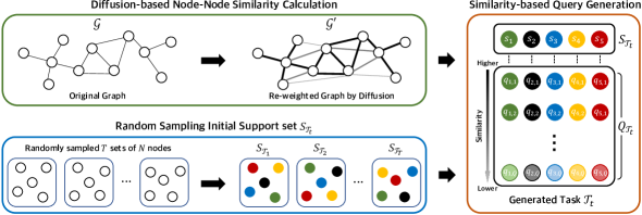
Figure 8. Overview of the NaQ-Diff. The only difference from NaQ-Feat is that NaQ-Diff utilizes graph diffusion instead of cosine similarity to get node-node similarity.

For this reason, we present another version of NaQ, named as NaQ-Diff, which utilizes structurally similar nodes found by generalized graph diffusion (Gasteiger et al., 2019) as queries. Specifically, NaQ-Diff leverages diffusion matrix $\mathbf{S}=\Sigma^{\infty}_{k=0}\theta_{k}\mathbf{T}^{k}$ as a similarity matrix, with the weighting coefficients $\theta_{k}$, and the generalized transition matrix $\mathbf{T}$. As edge weights of the diffusion matrix $\mathbf{S}$ can be interpreted as structural closeness, we can sample similar nodes of each support set node from $\mathbf{S}$. It is important to note that diffusion does not require additional computation during training as the diffusion matrix can be readily computed before the model training. Last but not least, although there can be other approaches for capturing the graph structural information (e.g., using the adjacency matrix, or using a k-NN graph computed based on node embeddings learned by a GNN encoder) (Lee et al., 2022a), we choose the graph diffusion as it captures more global information than the adjacency matrix, and computationally more efficient than the k-NN approach. The overview of NaQ-Diff can be found in Figure 8 in the Appendix and detailed setting for NaQ-Diff can be found in Section A.1 in Appendix. From now on, we call the former version of NaQ as NaQ-Feat and the latter version as NaQ-Diff when we have to distinguish them.

3.3. Model Training with Episodes from NaQ

In this section, we explain how to train existing meta-learning models with episodes generated by NaQ. However, due to the space limitation, we only describe how to train ProtoNet (Snell et al., 2017), which is one of the most widely used meta-learning models. Let $f_{\theta}$ be a GNN encoder, $\mathcal{T}_{t}$ be a generated episode, and $S_{\mathcal{T}_{t}}=\{(x^{spt}_{t,i},y^{spt}_{t,i})\}_{i=1}^{N\times 1}$ be a randomly sampled support set, then query set is generated as:

$$\small Q_{\mathcal{T}_{t}}=\{(x^{qry}_{t,i},y^{qry}_{t,i})\}_{i=1}^{N\times Q}=\mathrm{NaQ}(S_{\mathcal{T}_{t}}).$$

It is worth noting that since we only focus on query generation rather than support generation, we have a $N$-way 1-shot support set (i.e., $K=1$).

We first compute the prototype $\mathbf{c}_{j}$ of each class $j\in\{1,\cdots,N\}$ based on the support set as follows:

(2) $$\small\mathbf{c}_{j}=\frac{1}{K}\sum\nolimits_{i=1}^{K}f_{\theta}(x_{i})\cdot\mathbb{I}\{y_{i}=j\}\quad j=1,\cdots,N,$$

where $\mathbb{I}\{y_{i}=j\}$ is an indicator function that is equal to 1 only if the label $y_{i}$ of $x_{i}$ is $j$, otherwise 0. Then, for each query $q\in Q_{\mathcal{T}}$, where $q=(x_{q},y_{q})$, we obtain a distribution over $N$ classes as follows:

(3) $$\small P(y=j;q)=\frac{\mathrm{exp}(-d(f_{\theta}(x_{q}),\ \mathbf{c}_{j}))}{\sum_{j^{\prime}}\mathrm{exp}(-d(f_{\theta}(x_{q}),\ \mathbf{c}_{j^{\prime}}))}\quad j=1,\cdots,N,$$

where $d(\cdot,\cdot)$ is a distance function.

Then, the parameter is updated as: $\theta\leftarrow\theta-\eta\nabla_{\theta}\mathcal{L}(\theta;q)$, where $\eta$ is the learning rate and $\mathcal{L}(\theta;q)$ is a loss function given as:

$$\small\mathcal{L}(\theta;q)=-\frac{1}{N\times Q}\sum\nolimits_{q\in Q_{\mathcal{T}}}\mathrm{log}(P(y=j;q)).$$

Note that MAML (Finn et al., 2017), which is another widely used meta-learning model, is trained in a similar manner, while applying NaQ to some other existing models (e.g., TENT (Wang et al., 2022)) that utilize the entire labeled data $(X_{C_{b}},Y_{C_{b}})$ to compute cross-entropy loss along with episode-specific losses computed with training episodes per each update is non-trivial. Therefore, when such models are combined with our NaQ, cross-entropy loss calculated over $C_{b}$ is replaced with cross-entropy loss calculated over a single episode. With the exception mentioned above, since our proposed NaQ generates episodes in the same format as episodes made in a supervised manner, it can be directly combined with any of the existing meta-learning models almost without any modifications. It is important to note that since NaQ generates training episodes based on all nodes in a graph, NaQ enables the existing graph meta-learning methods to fully utilize the information of all nodes.

3.4. Brief Theoretical Considerations

In this section, we discuss why our NaQ works within the episodic learning framework by justifying our motivation of utilizing ‘similar’ nodes as queries presented in Section 3.1.

Due to the complicated model architecture of existing graph meta-learning methods, a thorough theoretical analysis of why our methods can work is far beyond the scope of this work. However, in some mathematical aspects, we can briefly investigate why our similarity-based episode generation methods work. To do so, we focus on the learning behavior of MAML (Finn et al., 2017) for a single episode during the training phase.

Let $f_{\theta}$ be a network parameterized by $\theta$, and $\mathcal{T}=(S_{\mathcal{T}},Q_{\mathcal{T}})$ be a given single training episode. We aim to learn unknown perfect estimation $f_{\mathcal{T}}$ using the training dataset (i.e., support set) $S_{\mathcal{T}}=\{(x_{i},y_{i})\}^{N\times K}_{i=1}$. Here we assume that the relationship between input $x$ and output $y$ is given by $y=f_{\mathcal{T}}(x)+\epsilon$, where $\epsilon$ is an irreducible error inherent in the observation, s.t. $\mathbb{E}[\epsilon]=0,\ \mathrm{Var}(\epsilon)=\sigma^{2}<\infty$.

To train the model on the episode $\mathcal{T}$, we fit $f_{\theta}$ on the given $S_{\mathcal{T}}$. However, as the support set $S_{\mathcal{T}}$ contains only a small amount of labeled samples (i.e., basic information) for the task $\mathcal{T}$, parameter update to $\theta^{\prime}=\mathrm{argmin}_{\theta}\sum_{(x_{i},y_{i})\in S_{\mathcal{T}}}\mathcal{L}\big{(}y_{i},f_{\theta}(x_{i})\big{)}$ might be problematic. More precisely, more than one solution $\theta^{\prime}$ can exist for the above minimization problem.

To enable better training on $\mathcal{T}$, additional information (i.e., query set $Q_{\mathcal{T}}$) is provided to make the model understand the training episode $\mathcal{T}$ better during the episodic learning. Formally, we can interpret this process as minimizing the generalization error of the fitted model $f_{\theta^{\prime}}$ on the query set (Khodadadeh et al., 2019). Without loss of generality, we only consider a single query $q=(x_{q},y_{q})\in Q_{\mathcal{T}}$. Thus, the estimate of generalization error on this point is $\mathcal{L}\big{(}y_{q},f_{\theta^{\prime}}(x_{q};S_{\mathcal{T}})\big{)}$. If we consider the case that $\mathcal{L}$ is the mean squared error, with abbreviation $f_{\theta^{\prime}}(\ \cdot\ )=f_{\theta^{\prime}}(\ \cdot\ ;S_{\mathcal{T}})$, we can decompose expected generalization error as follows (Gareth et al., 2013; Hastie et al., [n. d.]):

$$\small\mathbb{E}[\mathcal{L}\big{(}y_{q},f_{\theta^{\prime}}(x_{q})\big{)}]= \ \big{(}\mathbb{E}[f_{\theta^{\prime}}(x_{q})]-f_{\mathcal{T}}(x_{q})\big{)}^{2}$$

(4) $$+\Big{(}\mathbb{E}\big{[}f_{\theta^{\prime}}(x_{q})^{2}\big{]}-\mathbb{E}[f_{\theta^{\prime}}(x_{q})]^{2}\Big{)}+\sigma^{2}.$$

Since this generalization error estimate is used as a loss function to update our model, an accurate error estimation is essential to train our model $f_{\theta}$ on $\mathcal{T}$ better during the meta-training phase (Khodadadeh et al., 2019).

For this reason, during the query generation process of NaQ, it is crucial to discover class-level similar query $q=(x_{q},y_{q})$ for each support set sample $(x_{i},y_{i})\in S_{\mathcal{T}}$ for an accurate error estimation. Let $\tilde{y}_{q}$ and $\tilde{y}_{i}$ be true labels of discovered query $q$ and the corresponding support set sample $(x_{i},y_{i})$. Since we set pseudo-labels of the query and the corresponding support set sample to be equal (i.e., $y_{q}=y_{i}$), satisfying this class-level similarity condition, i.e., finding the query $q$ whose true label $\tilde{y}_{q}$ is similar enough to the true label $\tilde{y}_{i}$ of the corresponding support set sample $(x_{i},y_{i})$, is essential. Otherwise, this ‘label noise’ will introduce significant bias on the error estimate. Thus, in the end, we would fail to learn $f_{\mathcal{T}}$ by $f_{\theta}$.

In our conjecture, the analyses on the other models utilizing episodic learning framework might be similarly conducted, and similar results will be derived for the case of other loss functions, as the above analysis mainly considers the ‘label noise’ problem, which possibly happens during the query generation phase of NaQ. For example, in the case of ProtoNet (Snell et al., 2017), although it does not include the initial parameter update process as MAML we may analyze analogously by regarding $f_{\theta^{\prime}}(\ \cdot\ ;S_{\mathcal{T}})$ in the above analysis as the class prototype-query distance vector $\mathbf{p}_{j}=P(y=j;q)$ calculated from Equation 2 and 3. Although additional analyses on other episodic learning-based models are simplified or omitted due to the space limitation, we expect these analyses to explain the motivation of NaQ and why it can work.

4. Experiments

4.1. Experimental Settings

Evaluation Datasets

We used four benchmark datasets that are widely used in FSNC to comprehensively evaluate the performance of our unsupervised episode generation method. Two datasets (Amazon-Clothing (McAuley et al., 2015), Amazon-Electronics (McAuley et al., 2015)) are product networks and the other two datasets (Cora-Full (Bojchevski and Günnemann, 2018), DBLP (Tang et al., 2008)) are citation networks. Detailed explanation on evaluation datasets are provided in Section A.2 in the Appendix. The detailed statistics of the datasets can be found in Table 1. “Hom. ratio” denotes the homophily ratio of each dataset, and “Class split” denotes the number of distinct classes used to generate episodes in training (only for supervised settings), validation, and testing phase, respectively.

Baselines

We used four graph meta-learning models as baselines, i.e., MAML (Finn et al., 2017), ProtoNet (Snell et al., 2017), G-Meta (Huang and Zitnik, 2020) and TENT (Wang et al., 2022), to evaluate the performance of our unsupervised episode generation methods, i.e., NaQ-Feat and NaQ-Diff. In addition, three recent GCL baselines, i.e., BGRL (Thakoor et al., 2022), SUGRL (Mo et al., 2022) and AFGRL (Lee et al., 2022b), are included as they have shown remarkable performance on the FSNC task without using labels (Tan et al., [n. d.]). Lastly, VNT (Tan et al., 2023) is also included as a baseline. Detailed explanation on compared baselines are presented in Section A.3 in the Appendix.

For meta-learning baselines, we used a 2-layer GCN (Welling and Kipf, 2017) as the GNN encoder with the hidden dimension chosen from {64, 256}, and this makes MAML to be essentially equivalent to Meta-GNN (Zhou et al., 2019). Such choice of high hidden dimension size is based on (Chen et al., 2019), which demonstrated that a larger encoder capacity leads to a higher performance of meta-learning model. For each baseline, we tune hyperparameters for each episode generation method. For both NaQ-Feat and NaQ-Diff, we sampled $Q=10$ queries for each support set sample. For GCL baselines, we also used a 2-layer GCN encoder with the hidden dimension of size 256. For VNT, following the original paper, Graph-Bert (Zhang et al., 2020) is used as the backbone transformer model. As the official code of VNT is not available, we tried our best to reproduce VNT with the settings presented in the paper of VNT and Graph-Bert. For all baselines, Adam (Kingma and Ba, 2015) optimizer is used. The tuned parameters and their ranges are summarized in Table 4 in the Appendix.

Table 1. Dataset statistics.

Dataset	# Nodes	# Edges	# Features	# Labels	Class split	Hom. ratio
Amazon-Clothing	24,919	91,680	9,034	77	40/17/20	0.62
Amazon-Electronics	42,318	43,556	8,669	167	90/37/40	0.38
Cora-Full	19,793	65,311	8,710	70	25/20/25	0.59
DBLP	40,672	288,270	7,202	137	80/27/30	0.29

Evaluation

For each dataset except for Amazon-Clothing, we evaluate the performance of the models in 5/10/20-way, 1/5-shot settings (total 6 settings). For Amazon-Clothing, as the validation set contains 17 classes, evaluations on 20-way cannot be conducted. Instead, the evaluation is done in 5/10-way 1/5-shot settings (total 4 settings). In the validation and testing phases, we sampled 50 validation tasks and 500 testing tasks for all settings with 8 queries each. For all the baselines, validation/testing tasks are fixed, and we use linear probing on frozen features to solve each downstream task except VNT as it uses different strategy for solving downstream tasks. We report the average accuracy and 95% confidence interval over sampled testing tasks.

Table 2. Overall averaged FSNC accuracy (%) with 95% confidence intervals on product networks (Full ver. available at: Table 5)

Dataset

Amazon-Clothing

Amazon-Electronics

Setting

5 way

10 way

Avg. Rank

5 way

10 way

20 way

Avg. Rank

Baselines

1 shot

5 shot

1 shot

5 shot

1 shot

5 shot

1 shot

5 shot

1 shot

5 shot

MAML (Sup.)

76.13±1.17

84.28±0.87

63.77±0.83

76.95±0.65

8.50

65.58±1.26

78.55±0.96

57.31±0.87

67.56±0.73

46.37±0.61

60.04±0.52

7.50

ProtoNet (Sup.)

75.52±1.12

89.76±0.70

65.50±0.82

82.23±0.62

6.25

69.48±1.22

84.81±0.82

57.67±0.85

75.79±0.67

48.41±0.57

67.31±0.47

4.50

TENT (Sup.)

79.46±1.10

89.61±0.70

69.72±0.80

84.74±0.59

4.25

72.31±1.14

85.25±0.81

62.13±0.83

77.32±0.67

52.45±0.60

69.39±0.50

2.00

G-Meta (Sup.)

78.67±1.05

88.79±0.76

65.30±0.79

80.97±0.59

6.50

72.26±1.16

84.44±0.83

61.32±0.86

74.92±0.71

50.39±0.59

65.73±0.48

4.17

TLP-BGRL

81.42±1.05

90.53±0.71

72.05±0.86

83.64±0.63

3.50

64.20±1.10

81.72±0.85

53.16±0.82

73.70±0.66

44.57±0.54

65.13±0.47

6.83

TLP-SUGRL

63.32±1.19

86.35±0.78

54.81±0.77

73.10±0.63

9.50

54.76±1.06

78.12±0.92

46.51±0.80

68.41±0.71

36.08±0.52

57.78±0.49

9.67

TLP-AFGRL

78.12±1.13

89.82±0.73

71.12±0.81

83.88±0.63

4.50

59.07±1.07

81.15±0.85

50.71±0.85

73.87±0.66

43.10±0.56

65.44±0.48

7.17

VNT

65.09±1.23

85.86±0.76

62.43±0.81

80.87±0.63

8.75

56.69±1.22

78.02±0.97

49.98±0.83

70.51±0.73

42.10±0.53

60.99±0.50

8.83

NaQ-Feat (Ours)

86.58±0.96

92.27±0.67

79.55±0.78

86.10±0.60

1.00

76.46±1.11

88.72±0.73

69.59±0.86

81.44±0.61

59.65±0.60

74.60±0.47

1.00

NaQ-Diff (Ours)

82.27±1.10

90.82±0.68

72.67±0.82

84.54±0.61

2.25

69.62±1.20

84.88±0.83

60.44±0.79

76.73±0.67

51.44±0.58

68.37±0.49

3.33

Table 3. Overall averaged FSNC accuracy (%) with 95% confidence intervals on citation networks (Full ver. available at: Table 6)

Dataset	Cora-full							DBLP
Setting	5 way		10 way		20 way		Avg. Rank	5 way		10 way		20 way		Avg. Rank
Baselines	1 shot	5 shot	1 shot	5 shot	1 shot	5 shot		1 shot	5 shot	1 shot	5 shot	1 shot	5 shot
MAML (Sup.)	59.28±1.21	70.30±0.99	44.15±0.81	57.59±0.66	30.99±0.43	46.80±0.38	8.67	72.48±1.22	80.30±1.03	60.08±0.90	69.85±0.76	46.12±0.53	57.30±0.48	7.67
ProtoNet (Sup.)	58.61±1.21	73.91±0.93	44.54±0.79	62.15±0.64	32.10±0.42	50.87±0.40	7.17	73.80±1.20	81.33±1.00	61.88±0.86	73.02±0.74	48.70±0.52	62.42±0.45	3.83
TENT (Sup.)	61.30±1.18	77.32±0.81	47.30±0.80	66.40±0.62	36.40±0.45	55.77±0.39	4.00	74.01±1.20	82.54±1.00	62.95±0.85	73.26±0.77	49.67±0.53	61.87±0.47	2.33
G-Meta (Sup.)	59.88±1.26	75.36±0.86	44.34±0.80	59.59±0.66	33.25±0.42	49.00±0.39	7.00	74.64±1.20	79.96±1.08	61.50±0.88	70.33±0.77	46.07±0.52	58.38±0.47	6.33
TLP-BGRL	62.59±1.13	78.80±0.80	49.43±0.79	67.18±0.61	37.63±0.44	56.26±0.39	3.00	73.92±1.19	82.42±0.95	60.16±0.87	72.13±0.74	47.00±0.53	60.57±0.45	4.67
TLP-SUGRL	55.42±1.08	76.01±0.84	44.66±0.74	63.69±0.62	34.23±0.41	52.76±0.40	5.83	71.27±1.15	81.36±1.02	58.85±0.81	71.02±0.78	45.71±0.49	59.77±0.45	7.50
TLP-AFGRL	55.24±1.02	75.92±0.83	44.08±0.70	64.42±0.62	33.88±0.41	53.83±0.39	6.67	71.18±1.17	82.03±0.94	58.70±0.86	71.14±0.75	45.99±0.53	60.31±0.45	7.17
VNT	47.53±1.14	69.94±0.89	37.79±0.69	57.71±0.65	28.78±0.40	46.86±0.40	9.67	58.21±1.16	76.25±1.05	48.75±0.81	66.37±0.77	40.10±0.49	55.15±0.46	10.00
NaQ-Feat (Ours)	65.79±1.21	79.42±0.80	51.78±0.75	68.87±0.60	40.36±0.46	58.48±0.40	1.83	72.85±1.20	82.34±0.94	60.70±0.87	72.36±0.73	47.30±0.53	61.61±0.46	4.50
NaQ-Diff (Ours)	65.30±1.08	79.66±0.79	51.80±0.78	69.34±0.63	40.76±0.49	59.35±0.40	1.17	76.58±1.18	82.86±0.95	64.31±0.87	74.06±0.75	51.62±0.54	63.05±0.45	1.00

4.2. Overall Performance

The overall experimental results on four evaluation datasets are presented in Table 2 and 3. Note that as NaQ can be applied to any existing graph meta-learning models, i.e., MAML, ProtoNet, TENT, and G-Meta, we report the best performance among them. We have the following observations.

First, our proposed methods outperform the existing supervised baselines. We attribute these results to NaQ’s ability to extensively utilize nodes across the entire graph and NaQ’s flexible episode generation without label dependence. It is worth noting again that our methods have generated 1-shot training episodes while others used 5-shot training episodes. Thus, we expect that our method can be further improved if we develop methods to generate additional support set samples. We leave this as a future work.

Second, our proposed methods outperform methods utilizing the pre-trained encoder in an unsupervised manner (i.e., GCL methods and VNT). By applying the episodic learning framework for model training, our methods can capture information regarding the downstream task ‘format’ during the model training, leading to better performance in general.

Third, NaQ-Diff outperforms NaQ-Feat in citation networks as expected (See Table 3). This result validates our motivation for presenting NaQ-Diff in Section 3.2.1. On the other hand, NaQ-Feat outperforms NaQ-Diff in product networks. This is because it cannot be assured that products in ‘also-viewed’ or ‘bought-together’ relationships are similar or related products in the case of product networks (Zhang et al., 2022). For example, a TV and refrigerator can be ‘bought together’ when we move to a new house. In this case, discovering query sets based on ‘raw-feature’ similarity is more beneficial; thus, the result that NaQ-Feat $>$ NaQ-Diff in product networks can be validated.

In summary, NaQ can resolve the label-scarcity problem of supervised graph meta-learning methods and achieve performance enhancement on FSNC tasks by providing training episodes that contain both the information of all nodes in the graph, and the information of the downstream task format to the model.

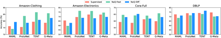
Figure 3. Model-agnostic property of NaQ for each dataset (5-way 1-shot)

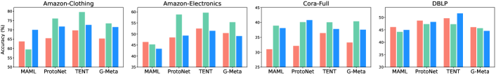
Figure 4. Model-agnostic property of NaQ in higher way settings (Amazon-Clothing: 10-way 1-shot, Others: 20-way 1-shot)

4.3. NaQ is model-agnostic

In this section, we provide experimental results to verify that NaQ can be applied to any existing graph meta-learning models while not much sacrificing their performance.

In Figure 3 and 4, we observe that our methods retained or even improved the performance of existing graph meta-learning methods across various few-shot settings with a few exceptions. Particularly, in higher-way settings shown in Figure 4, which are more challenging, ours generally outperform supervised methods. Therefore, we argue that our methods allow existing graph meta-learning algorithms to generate more generalizable embeddings without any use of label information. Moreover, the superior performance of NaQ with TENT is especially noteworthy as it outperforms vanilla supervised TENT even with much less data involved in training.

Lastly, it is important to note again that the performances of the supervised models reported in our experiments are only achievable when they have access to all labeled samples of entire base classes and given labeled samples in the base classes are clean. On the other hand, as shown in Figure 1(a) and 1(b), when there is inherent label noise in the base classes (Figure 1(a)) or there are only a limited amount of labeled samples within a limited number of base classes (Figure 1(b)), the performance of supervised models severely drops, while our unsupervised methods would not be affected at all. Furthermore, as will be demonstrated in Section 6, the performance of our methods can be improved by adjusting the number of queries.

5. Regarding ‘class-level similarity’

5.1. Why is ‘class-level similarity’ sufficient?

In Section 3.4, we justified our ‘similarity’ condition presented in Section 3.1 in terms of ‘class-level similarity’. In this section, we provide an explanation on why considering the class-level similarity (rather than the exact same class) condition is sufficient for the query generation process in NaQ, and further justify why our method outperforms supervised meta-learning methods.

Overall, we conjecture that training a model via episodic learning with episodes generated from NaQ can be done successfully not only because our methods enable utilization of the information of all nodes in the graph, but also because our methods generate sufficiently informative episodes that enable the model to learn the downstream task format based on the flexible episode generation. Here, the term ‘flexible’ is used in the context that the query generation of NaQ is not restricted to finding queries that have the exactly same label as the corresponding support set sample. Note that due to the nature of episodic learning we do not have to adhere to the condition that labels of queries and labels of their support set samples should be the same. Specifically, unlike the conventional training scheme, episodic learning only requires the model to classify $N$ classes given in a single episode among the total $|C|$ classes. For this reason, finding class-level similar queries is sufficient for generating informative training episodes.

Moreover, if we can generate training episodes that have queries similar enough to the corresponding support set sample while being dissimilar to the remaining $N-1$ support set samples, we further conjecture that the episodes utilizing class-level similar queries from NaQ is even more beneficial than episodes generated in ordinary supervised manner. This is because the episodes generated by NaQ provide helpful information from different but similar classes (i.e., classes of the queries from NaQ), while episodes generated in supervised way merely provide the information within the same classes as support set sample. To further demonstrate that NaQ has the ability to discover such class-level similar queries, empirical analysis is provided in Section 5.2.

5.2. NaQ discovers ‘class-level similar’ queries

In this section, we provide empirical evidence that NaQ can find class-level similar neighbors as queries for each support set sample (Figure 5), and we further analyze the experimental results of our methods based on that evidence.

To verify that queries found by NaQ are class-level similar, we measure the averaged class-level similarity between a node and its top-10 similar nodes found by feature similarity (NaQ-Feat) and graph diffusion (NaQ-Diff) in all four datasets. With node feature $X$, centroid $\mathbf{a}_{c}$ is obtained as $\mathbf{a}_{c}=\mathrm{MEAN}(\sum{x_{i}\cdot\mathbb{I}\{y_{i}=c\})}$ for each class $c\in C$, and then inter-class similarity between $c$ and $c^{\prime}\in C$ is calculated by cosine similarity between class centroids $\mathbf{a}_{c}$ and $\mathbf{a}_{c^{\prime}}$ (Tan et al., 2018). The results are presented in Figure 5. In most cases, similar nodes found by feature-level similarity or graph diffusion exhibit a high-level ($\sim$80%) average class-level similarity. This result shows that NaQ-Feat and NaQ-Diff can discover enough class-level similar nodes as queries for each support set sample.

In addition, we can further justify our arguments in Section 3.2.1 and the experimental results in Section 4.2 based on these results. First, we observe that we can sample more class-level similar queries by graph diffusion (NaQ-Diff) than raw-feature similarity (NaQ-Feat) in citation networks (i.e., Cora-Full and DBLP). Hence, considering graph structural information can be more beneficial in such cases. In addition, since NaQ-Diff can discover class-level similar queries in the DBLP dataset, it can show remarkable performance in the DBLP dataset even though DBLP has a low homophily ratio. Therefore, we emphasize again that discovering class-level similar queries is essential in generating informative episodes. Analogously, since we observe that one version of NaQ that shows better performance also has a higher class-level similarity in the corresponding dataset, we can analyse that making queries class-level similar to corresponding support set samples is directly related to the performance of NaQ.

In summary, we quantitatively demonstrated that NaQ indeed discovers class-level similar nodes without using label information, and we showed that the experimental results for our methods align well with our motivation regarding the support-query similarity, presented in Section 3.1 and justified in Section 3.4.

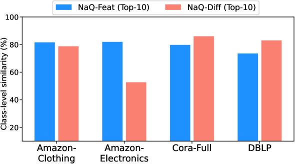
Figure 5. Averaged class-level similarity between each node and top-10 similar nodes found via NaQ-Feat and NaQ-Diff.

6. Model Analysis

Embedding Visualization. In this section, we present t-SNE (Van der Maaten and Hinton, 2008) plot to compare the quality of node embeddings by visualizing the embeddings of nodes from the target classes $C_{t}$. We randomly selected 5 target classes for the visualization on Amazon-Electronics dataset. We obtained node embeddings of NaQ from ProtoNet $+$ NaQ. As presented in Figure 6, we can observe that ours can improve the quality of embeddings of target class nodes. This result validates that NaQ enables the model to learn better embeddings by downstream task-aware training (i.e., episodic learning) with entire nodes involved in training.

Hyperparameter Sensitivity Analysis. So far, the experiments have been conducted with a fixed number of queries, $Q=10$. In this section, we investigate the effect of the number of queries on the performance of NaQ. To thoroughly explore the effect of the number of queries on NaQ, we check the performance of NaQ with ProtoNet by changing the number of queries $Q$ within {1, 3, 5, 7, 10, 13, 15, 17, 20, 30, 40, 100}. We have the following observations from Figure 7: (1) In Amazon-Clothing, since both NaQ-Feat and NaQ-Diff can discover highly class-level similar queries (See Figure 5), they exhibit an increasing tendency in performance as $Q$ increases. (2) In the case of Amazon-Electronics, NaQ-Feat shows a similar tendency as in Amazon-Clothing due to the same reason, while there is a slight performance drop when $Q=100$. In contrast, NaQ-Diff shows clearly decreasing performance after $Q=5$, as its queries have relatively low class-level similarity (See Figure 5). From the results above, we can conclude that sampling a proper number of queries $Q$ during the episode generation phase is essential. Otherwise, a significant level of label noise in the generated episode might hinder the model training. (3) In the DBLP dataset, NaQ-Feat shows a nearly consistent performance tendency, while the performance of NaQ-Diff can be enhanced by increasing the number of queries for training. This is because NaQ-Diff can sample more class-level similar queries than NaQ-Feat (See Figure 5). From this observation, we again validate the motivation of utilizing structural neighbors as queries in such a dataset (See Section 3.2.1).

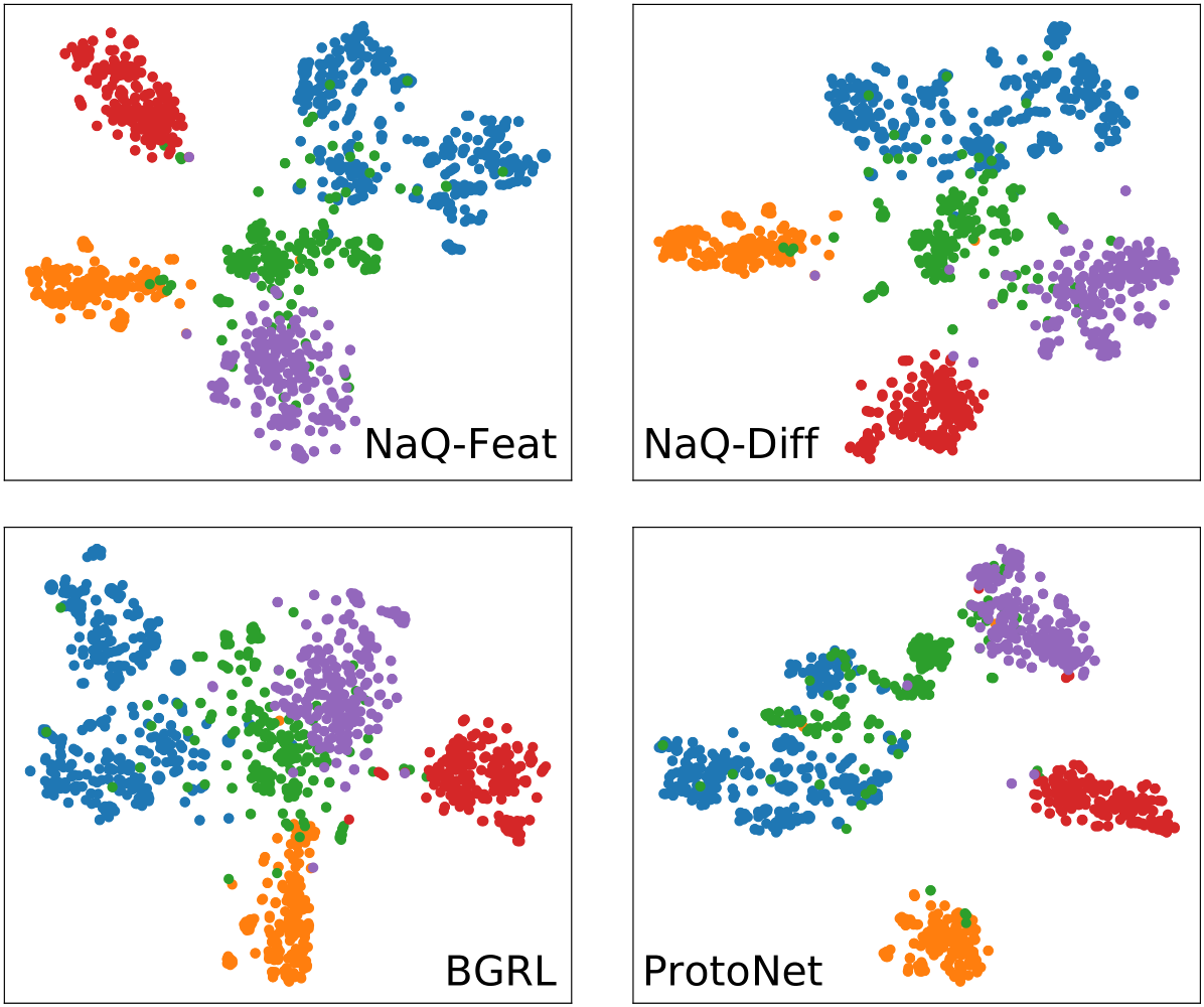
Figure 6. The t-SNE plot on Amazon-Electronics (5-way 1-shot, base-model: ProtoNet)

7. Related Work

7.1. Few-Shot Node Classification

Few-shot learning (FSL) (Vinyals et al., 2016; Finn et al., 2017; Snell et al., 2017) aims to classify unseen samples with only a few labeled samples based on the meta-knowledge obtained from training on abundant samples from base classes.

Graph Meta-learning Various efforts have recently been made to solve FSNC problem on graph-structured data. Meta-GNN (Zhou et al., 2019) addresses the problem by directly applying MAML with graph neural networks, and GPN (Ding et al., 2020) uses ProtoNet (Snell et al., 2017) architecture with adjusted prototype calculation by considering node importance. Furthermore, G-Meta (Huang and Zitnik, 2020) utilizes subgraph-level embeddings of nodes inside training episodes based on both ProtoNet and MAML (Finn et al., 2017) frameworks and enables scalable and inductive graph meta-learning. In addition, TENT (Wang et al., 2022) tries to reduce variances within training episodes through node-level, class-level, and task-level adaptations.

Unsupervised FSNC More recently, there were several studies to handle the FSNC problem in an unsupervised manner. TLP (Tan et al., [n. d.]) utilizes GCL methods, such as BGRL (Thakoor et al., 2022) and SUGRL (Mo et al., 2022), to solve FSNC problem, and it has shown remarkable success for FSNC problem without labels. VNT (Tan et al., 2023) applies graph transformer architecture on FSNC and solves the downstream FSNC task by only fine-tuning ‘virtual’ nodes injected as soft prompts and the classifier with given a few-labeled samples in the downstream task.

7.2. Unsupervised Meta-learning

In computer vision, several unsupervised meta-learning methods exist that attempt to address the limitations of requiring abundant labels for constructing training episodes. More precisely, UMTRA (Khodadadeh et al., 2019) and AAL (Antoniou and Storkey, 2019) are similar methods, making queries via image augmentation on randomly sampled support set samples. The significant difference between the two methods is that AAL makes support sets by grouping randomly sampled images into the same pseudo-classes, while UMTRA ensures those support set samples have different labels from each other. In addition, AAL focuses on task generation, while UMTRA is mainly applied to MAML. On the other hand, CACTUs (Hsu et al., 2018) aims to make episodes based on pseudo-labels obtained from cluster assignments, which come from features pre-trained in an unsupervised fashion. LASIUM (Khodadadeh et al., 2020) generates synthetic training episodes that can be combined with existing models, such as MAML and ProtoNet, with generative models. Moreover, Meta-GMVAE (Lee et al., 2021) uses VAE (Kingma and Welling, 2013) with Gaussian mixture priors to solve the few-shot learning problem.

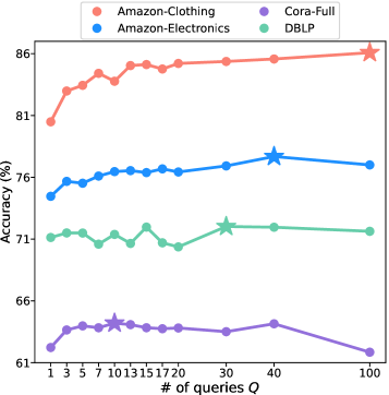
(a)

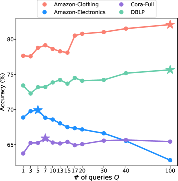
(b)

Figure 7. Effect of number of queries NaQ (5-way 1-shot, base-model: ProtoNet, star marker: maximal point)

8. Conclusion & Future work

In this work, we proposed NaQ, a novel unsupervised episode generation algorithm which generates 1) support sets via random sampling from the entire graph, and 2) query sets by utilizing feature-level similar nodes (i.e., NaQ-Feat) or structurally similar neighbors from graph diffusion (i.e., NaQ-Diff). As NaQ generates training episodes out of all nodes in the graph without any label information, it can address the label-scarcity problem of supervised graph meta-learning models. Moreover, generated episodes from NaQ can be used for training any existing graph meta-learning models almost without modifications and even boost their performance on the FSNC task. Extensive experimental studies on various downstream task settings demonstrate the superiority and potential of NaQ. As a future work, devising a more sophisticated support set generation method rather than naïve random sampling would be a promising direction, since random sampling may suffer from the false-negative problem.

Appendix A Appendix

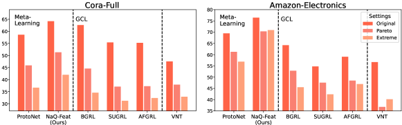
Figure 9. Impact of the class imbalance on 5-way 1-shot FSNC performance

A.1. Details on NaQ-Diff

For NaQ-Diff, we used personalized PageRank (Page et al., 1999)-based diffusion to obtain diffusion matrix $\mathbf{S}$, where $\theta^{PPR}_{k}=\alpha(1-\alpha)^{k}$, with teleport probability $\alpha\in(0,1)$, as weighting coefficient $\theta_{k}$. In our experiments, $\alpha=0.1$ is used to calculate PPR-based diffusion. Also, we used $\tilde{T}_{sym}=(w_{loop}\cdot\mathbf{I}_{N}+D)^{-1/2}(w_{loop}\cdot\mathbf{I}_{N}+A)(w_{loop}\cdot\mathbf{I}_{N}+D)^{-1/2}$, with the self-loop weight $w_{loop}=1$, as transition matrix, where $A\in\mathbb{R}^{|\mathcal{V}|\times|\mathcal{V}|}$ is an adjacency matrix of the graph $\mathcal{G}$ and $D$ is a diagonal matrix whose entries $D_{ii}=\sum_{j}A_{ij}$ are each node’s degree.

A.2. Details on Evaluation Datasets

The following is the details on evaluation datasets used in this work.

• Amazon-Clothing (McAuley et al., 2015) is a product-product network, whose nodes are products from the category “Clothing, Shoes and Jewelry” in Amazon. Node features are constructed from the product descriptions, and edges were created based on ”also-viewed” relationships between products. The node class is a low-level product category.

• Amazon-Electronics (McAuley et al., 2015) is a network of products, whose nodes are products from the category “Electronics” in Amazon. Node features are constructed from the product descriptions, and edges represent the “bought-together” relationship between products. The node class is a low-level product category.

• Cora-Full (Bojchevski and Günnemann, 2018) is a citation network, whose nodes are papers. The node features are constructed from a bag-of-words representation of each node’s title and abstract, and edges represent the citation relationship between papers. The node class is the paper topic.

• DBLP (Tang et al., 2008) is a citation network, whose nodes are papers. Node features are constructed from their abstracts, and edges represent the citation relationship between papers. The node class is the venue where the paper is published.

Table 4. Tuned hyperparameters and their range by baselines

Baselines	Hyperparameters and Range
MAML-like (MAML, G-Meta)	Inner step learning rate $\in\{0.01,0.05,0.1,0.3,0.5\}$, # of inner updates $\in\{1,2,5,10,20\}$, Meta-learning rate $\in\{0.001,0.003\}$
ProtoNet-like (ProtoNet, TENT)	Learning rate $\in\{5\cdot 10^{-5},10^{-4},\ 3\cdot 10^{-4},5\cdot 10^{-4},10^{-3},3\cdot 10^{-3},5\cdot 10^{-3}\}$
Self-Supervised (TLP)	Learning rate $\in\{10^{-6},10^{-5},5\cdot 10^{-5},10^{-4},5\cdot 10^{-4},10^{-3}\}$

Table 5. Overall averaged FSNC accuracy (%) with 95% confidence intervals on product networks (Full Version)

Dataset		Amazon-Clothing				Amazon-Electronics
Setting		5 way		10 way		5 way		10 way		20 way
Base Model	Episode Generation	1 shot	5 shot	1 shot	5 shot	1 shot	5 shot	1 shot	5 shot	1 shot	5 shot
MAML	Supervised	76.13±1.17	84.28±0.87	63.77±0.83	76.95±0.65	65.58±1.26	78.55±0.96	57.31±0.87	67.56±0.73	46.37±0.61	60.04±0.52
	g-UMTRA (Ours)	70.88±1.31	81.58±0.94	64.54±0.89	78.21±0.66	59.63±1.16	76.21±0.96	51.04±0.88	69.37±0.72	42.56±0.58	60.02±0.53
	NaQ-Feat (Ours)	74.07±1.07	86.49±0.86	59.44±0.91	75.99±0.70	59.56±1.17	74.85±1.03	49.03±0.88	70.47±0.73	45.27±0.60	62.36±0.51
	NaQ-Diff (Ours)	79.30±1.17	86.81±0.82	69.97±0.86	79.74±0.68	62.90±1.18	78.37±0.90	52.23±0.84	68.77±0.76	43.28±0.62	59.88±0.51
ProtoNet	Supervised	75.52±1.12	89.76±0.70	65.50±0.82	82.23±0.62	69.48±1.22	84.81±0.82	57.67±0.85	75.79±0.67	48.41±0.57	67.31±0.47
	g-UMTRA (Ours)	82.65±1.00	90.72±0.70	74.30±0.78	84.06±0.62	73.07±1.14	85.93±0.80	65.03±0.82	78.18±0.65	55.42±0.58	70.52±0.48
	NaQ-Feat (Ours)	83.77±0.96	92.27±0.67	76.08±0.81	85.60±0.60	76.46±1.11	88.72±0.73	68.42±0.86	81.36±0.64	58.80±0.60	74.60±0.47
	NaQ-Diff (Ours)	78.64±1.05	90.82±0.68	71.75±0.81	83.81±0.60	68.56±1.18	84.88±0.83	59.46±0.86	76.73±0.67	49.24±0.59	67.99±0.48
TENT	Supervised	79.46±1.10	89.61±0.70	69.72±0.80	84.74±0.59	72.31±1.14	85.25±0.81	62.13±0.83	77.32±0.67	52.45±0.60	69.39±0.50
	g-UMTRA (Ours)	78.55±1.14	89.80±0.72	72.00±0.82	84.30±0.59	67.57±1.19	81.73±0.88	61.04±0.83	75.70±0.68	50.99±0.59	68.40±0.48
	NaQ-Feat (Ours)	86.58±0.96	91.98±0.67	79.55±0.78	86.10±0.60	76.26±1.11	87.27±0.81	69.59±0.86	81.44±0.61	59.65±0.60	74.09±0.46
	NaQ-Diff (Ours)	80.87±1.08	90.53±0.71	72.67±0.82	84.54±0.61	68.14±1.13	83.64±0.80	60.44±0.79	76.03±0.67	51.44±0.58	68.37±0.49
G-Meta	Supervised	78.67±1.05	88.79±0.76	65.30±0.79	80.97±0.59	72.26±1.16	84.44±0.83	61.32±0.86	74.92±0.71	50.39±0.59	65.73±0.48
	g-UMTRA (Ours)	74.86±1.12	87.04±0.79	62.08±0.83	77.54±0.62	61.21±1.20	78.10±0.94	55.80±0.81	74.33±0.68	45.74±0.58	63.67±0.50
	NaQ-Feat (Ours)	85.83±1.03	90.70±0.73	73.45±0.84	82.61±0.66	74.49±1.15	84.68±0.86	61.18±0.83	77.36±0.67	55.35±0.60	69.16±0.51
	NaQ-Diff (Ours)	82.27±1.10	89.88±0.77	71.48±0.86	82.07±0.63	69.62±1.20	80.87±0.94	58.71±0.80	75.55±0.67	49.06±0.58	67.41±0.47
TLP	BGRL	81.42±1.05	90.53±0.71	72.05±0.86	83.64±0.63	64.20±1.10	81.72±0.85	53.16±0.82	73.70±0.66	44.57±0.54	65.13±0.47
	SUGRL	63.32±1.19	86.35±0.78	54.81±0.77	73.10±0.63	54.76±1.06	78.12±0.92	46.51±0.80	68.41±0.71	36.08±0.52	57.78±0.49
	AFGRL	78.12±1.13	89.82±0.73	71.12±0.81	83.88±0.63	59.07±1.07	81.15±0.85	50.71±0.85	73.87±0.66	43.10±0.56	65.44±0.48
VNT		65.09±1.23	85.86±0.76	62.43±0.81	80.87±0.63	56.69±1.22	78.02±0.97	49.98±0.83	70.51±0.73	42.10±0.53	60.99±0.50

Table 6. Overall averaged FSNC accuracy (%) with 95% confidence intervals on product networks (Full Version)

Dataset		Cora-full						DBLP
Setting		5 way		10 way		20 way		5 way		10 way		20 way
Base Model	Episode Generation	1 shot	5 shot	1 shot	5 shot	1 shot	5 shot	1 shot	5 shot	1 shot	5 shot	1 shot	5 shot
MAML	Supervised	59.28±1.21	70.30±0.99	44.15±0.81	57.59±0.66	30.99±0.43	46.80±0.38	72.48±1.22	80.30±1.03	60.08±0.90	69.85±0.76	46.12±0.53	57.30±0.48
	g-UMTRA (Ours)	53.80±1.19	68.47±1.01	42.08±0.79	55.46±0.65	24.02±0.37	42.09±0.40	66.43±1.24	77.37±1.03	52.29±0.89	68.10±0.77	40.53±0.53	56.38±0.49
	NaQ-Feat (Ours)	64.64±1.16	74.31±0.94	49.86±0.78	64.88±0.64	38.90±0.46	53.87±0.43	68.49±1.23	77.31±1.08	55.70±0.88	67.94±0.82	44.18±0.53	56.50±0.48
	NaQ-Diff (Ours)	62.93±1.17	76.48±0.92	50.10±0.83	63.50±0.66	38.09±0.45	54.08±0.41	71.14±1.15	79.47±1.01	59.18±0.91	70.19±0.78	44.94±0.57	58.68±0.47
ProtoNet	Supervised	58.61±1.21	73.91±0.93	44.54±0.79	62.15±0.64	32.10±0.42	50.87±0.40	73.80±1.20	81.33±1.00	61.88±0.86	73.02±0.74	48.70±0.52	62.42±0.45
	g-UMTRA (Ours)	61.69±1.17	77.00±0.87	51.09±0.78	66.44±0.62	36.70±0.43	53.05±0.40	71.68±1.18	80.93±1.01	60.28±0.82	70.53±0.78	47.33±0.53	61.60±0.45
	NaQ-Feat (Ours)	64.20±1.11	79.42±0.80	51.78±0.75	68.87±0.60	40.11±0.45	58.48±0.40	71.38±1.17	82.34±0.94	58.41±0.86	72.36±0.73	47.30±0.53	61.61±0.46
	NaQ-Diff (Ours)	65.30±1.08	79.66±0.79	51.80±0.78	69.34±0.63	40.76±0.49	59.35±0.40	73.89±1.15	82.24±0.98	59.43±0.79	72.85±0.76	48.17±0.52	61.66±0.48
TENT	Supervised	61.30±1.18	77.32±0.81	47.30±0.80	66.40±0.62	36.40±0.45	55.77±0.39	74.01±1.20	82.54±1.00	62.95±0.85	73.26±0.77	49.67±0.53	61.87±0.47
	g-UMTRA (Ours)	58.60±1.23	72.20±0.92	49.22±0.81	65.58±0.66	37.20±0.47	53.35±0.41	71.76±1.19	78.90±1.04	61.23±0.85	71.53±0.77	48.70±0.54	61.09±0.44
	NaQ-Feat (Ours)	64.04±1.14	78.48±0.79	51.31±0.77	67.09±0.62	40.04±0.48	56.15±0.40	72.85±1.20	80.91±1.00	60.70±0.87	71.98±0.79	47.29±0.53	61.01±0.46
	NaQ-Diff (Ours)	61.85±1.12	77.26±0.84	49.80±0.76	67.65±0.63	37.78±0.45	56.55±0.41	76.58±1.18	82.86±0.95	64.31±0.87	74.06±0.75	51.62±0.54	63.05±0.45
G-Meta	Supervised	59.88±1.26	75.36±0.86	44.34±0.80	59.59±0.66	33.25±0.42	49.00±0.39	74.64±1.20	79.96±1.08	61.50±0.88	70.33±0.77	46.07±0.52	58.38±0.47
	g-UMTRA (Ours)	44.25±1.00	64.27±0.95	35.36±0.73	53.68±0.65	24.26±0.39	44.74±0.41	68.64±1.28	80.31±0.97	55.19±0.87	69.85±0.73	44.06±0.53	59.72±0.46
	NaQ-Feat (Ours)	65.79±1.21	79.21±0.82	48.90±0.80	63.96±0.61	40.36±0.46	55.17±0.43	70.08±1.24	80.79±0.97	57.98±0.87	71.18±0.75	45.65±0.52	59.38±0.46
	NaQ-Diff (Ours)	62.96±1.14	77.31±0.87	47.93±0.79	63.18±0.61	37.55±0.46	54.23±0.41	70.39±1.20	80.47±1.03	57.55±0.85	69.59±0.78	44.56±0.52	58.66±0.45
TLP	BGRL	62.59±1.13	78.80±0.80	49.43±0.79	67.18±0.61	37.63±0.44	56.26±0.39	73.92±1.19	82.42±0.95	60.16±0.87	72.13±0.74	47.00±0.53	60.57±0.45
	SUGRL	55.42±1.08	76.01±0.84	44.66±0.74	63.69±0.62	34.23±0.41	52.76±0.40	71.27±1.15	81.36±1.02	58.85±0.81	71.02±0.78	45.71±0.49	59.77±0.45
	AFGRL	55.24±1.02	75.92±0.83	44.08±0.70	64.42±0.62	33.88±0.41	53.83±0.39	71.18±1.17	82.03±0.94	58.70±0.86	71.14±0.75	45.99±0.53	60.31±0.45
VNT		47.53±1.14	69.94±0.89	37.79±0.69	57.71±0.65	28.78±0.40	46.86±0.40	58.21±1.16	76.25±1.05	48.75±0.81	66.37±0.77	40.10±0.49	55.15±0.46

A.3. Details on Compared Baselines

Details on compared baselines are presented as follows.

• MAML (Finn et al., 2017) aims to find good initialization for downstream tasks. It optimizes parameters via two-phase optimization. The inner-loop update finds task-specific parameters based on the support set of each task, and the outer-loop update finds a good parameter initialization point based on the query set.

• ProtoNet (Snell et al., 2017) trains a model by building $N$ class prototypes by averaging support samples of each class, and making each query sample and corresponding prototype closer.

• G-Meta (Huang and Zitnik, 2020) obtains node embeddings based on the subgraph of each node in episodes, which allows scalable and inductive graph meta-learning.

• TENT (Wang et al., 2022) performs graph meta-learning to reduce task variance among training episodes via node-level, class-level, and task-level adaptations. When it is combined with our NaQs, cross-entropy loss calculated over $C_{b}$ is replaced with cross entropy loss calculated over a single episode.

• BGRL (Thakoor et al., 2022) applies BYOL (Grill et al., 2020) on graphs, so it trains the model by maximizing the agreement between an online embedding and a target embedding of each node, where each embedding is obtained from two differently augmented views.

• SUGRL (Mo et al., 2022) simplifies architectures for effective and efficient contrastive learning on graphs, and trains the model by concurrently increasing inter-class variation and reducing intra-class variation.

• AFGRL (Lee et al., 2022b) applies BYOL architecture without graph augmentations. Instead of augmentations, AFGRL generates another view by mining positive nodes in the graph in terms of both local and global perspectives.

• VNT (Tan et al., 2023) utilizes pretrained transformer-based encoder (Graph-Bert (Zhang et al., 2020)) as a backbone, and adapts to the downstream FSNC task by tuning injected ‘virtual’ nodes and classifier with given a few labeled samples in the downstream task, then makes prediction on queries with such fine-tuned virtual nodes and classifier.

Discussion on VNT Although we tried our best to reproduce VNT, we failed to achieve their performance especially on Cora-Full, an evaluation dataset shared by VNT and our paper. This might be due to the random seed, used evaluation data, or the transformer architecture used in the experiment. However, we conjecture it will also suffer from the inherent bias in data such as class imbalance similar to GCL methods, as graph transformer-based model also learn generic embedding by pretraining on a given graph. As evidence, experimental results on Cora-Full and Amazon-Electronics in the same setting as Figure 1(c), performance of VNT is also deteriorated like GCL methods (See Figure 9).

A.4. g-UMTRA: Augmentation-based Query Generation Method

Inspired by UMTRA (Khodadadeh et al., 2019), we devised an augmentation-based query generation method called g-UMTRA. as an investigation method. g-UMTRA generates query set by applying graph augmentation on the support set. The method overview an be found in Figure 10

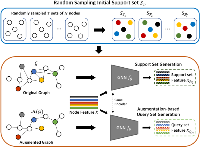
Figure 10. Overview of g-UMTRA. First, we randomly sample $T$ sets of $N$ nodes from the entire graph and assign them distinct labels. Then, we generate support set features by using a GNN encoder with original structures and query set features with augmented structures.

Specifically, we first randomly sample $T$ sets of $N$ nodes from entire graph to generate $\{\mathcal{T}_{t}\}_{t=1}^{T}$. Then for each task $\mathcal{T}_{t}$, we generate a $N$-way support set $S_{\mathcal{T}_{t}}=\{(x_{t,i},y_{t,i})\ |\ x_{t,i}\in\mathcal{V}\}_{i=1}^{N\times 1}$ with distinct pseudo-labels $y_{t,i}$ for each $x_{t,i}$, and their corresponding query set $Q_{\mathcal{T}_{t}}$ in the embedding space by applying graph augmentation.

By notating GNN encoder $f_{\theta}$ as $f_{\theta}(\mathcal{V};\mathcal{G})$, we can formally describe the query generation process of g-UMTRA as follows:

$$X_{S_{\mathcal{T}_{t}}} =\{\big{(}f_{\theta}(x_{t,i};\mathcal{G}),y_{t,i}\big{)}\ |\ (x_{t,i},y_{t,i})\in S_{\mathcal{T}_{t}}\},$$

(5) $$X_{Q_{\mathcal{T}_{t}}} =\{\big{(}f_{\theta}(x_{t,i};\mathcal{A}(\mathcal{G})),y_{t,i}\big{)}\ |\ (x_{t,i},y_{t,i})\in S_{\mathcal{T}_{t}}\},$$

where $f_{\theta}(x_{t,i};\mathcal{G})$ is an embedding of node $x_{t,i}$ with the given graph $\mathcal{G}$ and a GNN encoder $f_{\theta}$, and $\mathcal{A}(\cdot)$ is a graph augmentation function. For $\mathcal{A}(\cdot)$, we can consider various strategies such as node feature masking (DropFeature) or DropEdge (Rong et al., 2020).

Note that g-UMTRA is distinguished from UMTRA in the following two aspects: (1) g-UMTRA can be applied to any existing graph meta-learning methods as it only focuses on episode generation, while UMTRA is mainly applied on MAML. (2) As described in Equation A.4, g-UMTRA generates episodes as pair of sets $(X_{S_{\mathcal{T}_{j}}},X_{Q_{\mathcal{T}_{j}}})$ that consist of embeddings. Hence, its query generation process should take place in the training process, since augmentation and embedding calculation of GNNs depend on the graph structure. However, in UMTRA, image augmentation and ordinary convolutional neural networks are applied in instance-level, implying that the episode generation process of UMTRA can be done before training.

As described in Table 5 and 6, g-UMTRA can show competitive performance on FSNC. However, since it requires additional computation of augmented embedding by each update, which is time-consuming, as graph augmentation has to be applied across the entire graph. Moreover, since it uses graph augmentation and only sampled support set itself to generate queries, it requires inevitable modification on the training process of some existing models like G-Meta and TENT, up-to-date graph meta-learning methods which are developed under the premise of utilizing supervised episodes, having mutually exclusive support set and query set. For this reason, mainly considered similarity-based query sampling algorithm named NaQ during the research process, which is easily applicable to existing models and shows great performance improvement across the dataset.

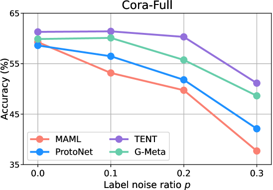
Figure 11. Impact of label noise on supervised graph meta-learning models in Cora-Full dataset (5-way 1-shot)

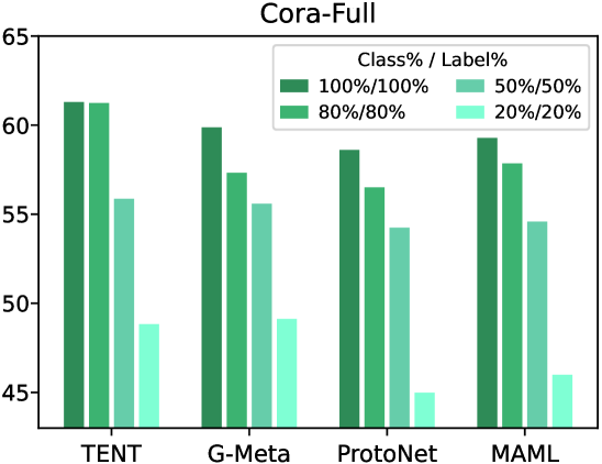
Figure 12. Impact of label-scarcity on supervised graph meta-learning models in Cora-Full dataset (5-way 1-shot)

A.5. Additional Experimental Results

A.5.1. Impact of the label noise on supervised models

We also conducted experiment regarding label noise presented in Figure 1(a) for Cora-Full dataset. Note that as Cora-Full has smaller size than Amazon-Electronics, we selected label noise $p$ ratio from $\{0,0.1,0.2,0.3\}$. As shown in Figure 11, similar to the result in Figure 1(a), supervised meta-learning models still exhibit degrading performance as noise level increases.

A.5.2. Impact of the label-scarcity on supervised models

We also conducted experiment presented in Figure 1(b) for Cora-Full dataset. Similar to the result in Figure 1(b), supervised graph meta-learning models’ FSNC performance decreases as available labeled data and diversity of base classes decrease (See Figure 12).

A.5.3. Impact of the class imbalance

We also conducted experiment presented in Figure 1(c) for Cora-Full dataset. The results can be found in Figure 9. Similar to the result in Figure 1(c), meta-learning methods including ours still outperform the other methods in all settings.

References

- (1)
- Antoniou and Storkey (2019) Antreas Antoniou and Amos Storkey. 2019. Assume, augment and learn: Unsupervised few-shot meta-learning via random labels and data augmentation. arXiv preprint arXiv:1902.09884 (2019).
- Bojchevski and Günnemann (2018) Aleksandar Bojchevski and Stephan Günnemann. 2018. Deep Gaussian Embedding of Graphs: Unsupervised Inductive Learning via Ranking. In International Conference on Learning Representations.
- Chen et al. (2019) Wei-Yu Chen, Yen-Cheng Liu, Zsolt Kira, Yu-Chiang Frank Wang, and Jia-Bin Huang. 2019. A closer look at few-shot classification. arXiv preprint arXiv:1904.04232 (2019).
- Ding et al. (2020) Kaize Ding, Jianling Wang, Jundong Li, Kai Shu, Chenghao Liu, and Huan Liu. 2020. Graph prototypical networks for few-shot learning on attributed networks. In Proceedings of the 29th ACM International Conference on Information & Knowledge Management. 295–304.
- Finn et al. (2017) Chelsea Finn, Pieter Abbeel, and Sergey Levine. 2017. Model-Agnostic Meta-Learning for Fast Adaptation of Deep Networks. In Proceedings of the 34th International Conference on Machine Learning, Vol. 70. PMLR, 1126–1135.
- Gareth et al. (2013) James Gareth, Witten Daniela, Hastie Trevor, and Tibshirani Robert. 2013. An introduction to statistical learning: with applications in R. Springer.
- Gasteiger et al. (2019) Johannes Gasteiger, Stefan Weißenberger, and Stephan Günnemann. 2019. Diffusion Improves Graph Learning. Advances in Neural Information Processing Systems 32 (2019).
- Grill et al. (2020) Jean-Bastien Grill, Florian Strub, Florent Altché, Corentin Tallec, Pierre H. Richemond, Elena Buchatskaya, Carl Doersch, Bernardo Avila Pires, Zhaohan Daniel Guo, Mohammad Gheshlaghi Azar, Bilal Piot, Koray Kavukcuoglu, Rémi Munos, and Michal Valko. 2020. Bootstrap your own latent: A new approach to self-supervised Learning. NeurIPS (2020).
- Hastie et al. ([n. d.]) Trevor Hastie, Robert Tibshirani, and Jerome Friedman. [n. d.]. The elements of statistical learning: data mining, inference, and prediction. Vol. 2. Springer.
- Hsu et al. (2018) Kyle Hsu, Sergey Levine, and Chelsea Finn. 2018. Unsupervised learning via meta-learning. arXiv preprint arXiv:1810.02334 (2018).
- Huang and Zitnik (2020) Kexin Huang and Marinka Zitnik. 2020. Graph meta learning via local subgraphs. Advances in Neural Information Processing Systems 33 (2020).
- Jin et al. (2020) Wei Jin, Yao Ma, Xiaorui Liu, Xianfeng Tang, Suhang Wang, and Jiliang Tang. 2020. Graph structure learning for robust graph neural networks. In Proceedings of the 26th ACM SIGKDD international conference on knowledge discovery & data mining. 66–74.
- Khodadadeh et al. (2019) Siavash Khodadadeh, Ladislau Boloni, and Mubarak Shah. 2019. Unsupervised meta-learning for few-shot image classification. Advances in neural information processing systems 32 (2019).
- Khodadadeh et al. (2020) Siavash Khodadadeh, Sharare Zehtabian, Saeed Vahidian, Weijia Wang, Bill Lin, and Ladislau Bölöni. 2020. Unsupervised meta-learning through latent-space interpolation in generative models. arXiv preprint arXiv:2006.10236 (2020).
- Kim et al. (2023) Sungwon Kim, Junseok Lee, Namkyeong Lee, Wonjoong Kim, Seungyoon Choi, and Chanyoung Park. 2023. Task-Equivariant Graph Few-shot Learning. In Proceedings of the 29th ACM SIGKDD Conference on Knowledge Discovery and Data Mining. 1120––1131.
- Kingma and Ba (2015) Diederik P. Kingma and Jimmy Lei Ba. 2015. Adam: A Method for Stochastic Optimization. In International Conference on Learning Representations.
- Kingma and Welling (2013) Diederik P Kingma and Max Welling. 2013. Auto-encoding variational bayes. arXiv preprint arXiv:1312.6114 (2013).
- Lee et al. (2021) Dong Bok Lee, Dongchan Min, Seanie Lee, and Sung Ju Hwang. 2021. Meta-gmvae: Mixture of gaussian vae for unsupervised meta-learning. In International Conference on Learning Representations.
- Lee et al. (2022a) Namkyeong Lee, Dongmin Hyun, Junseok Lee, and Chanyoung Park. 2022a. Relational self-supervised learning on graphs. In Proceedings of the 31st ACM International Conference on Information & Knowledge Management. 1054–1063.
- Lee et al. (2022b) Namkyeong Lee, Junseok Lee, and Chanyoung Park. 2022b. Augmentation-free self-supervised learning on graphs. In Proceedings of the AAAI Conference on Artificial Intelligence, Vol. 36. 7372–7380.
- McAuley et al. (2015) Julian McAuley, Rahul Pandey, and Jure Leskovec. 2015. Inferring networks of substitutable and complementary products. In Proceedings of the 21th ACM SIGKDD international conference on knowledge discovery and data mining. 785–794.
- McPherson et al. (2001) Miller McPherson, Lynn Smith-Lovin, and James M Cook. 2001. Birds of a feather: Homophily in social networks. Annual review of sociology 27, 1 (2001), 415–444.
- Mo et al. (2022) Yujie Mo, Liang Peng, Jie Xu, Xiaoshuang Shi, and Xiaofeng Zhu. 2022. Simple Unsupervised Graph Representation Learning. In Proceedings of the AAAI Conference on Artificial Intelligence (AAAI). 7797–7805.
- Page et al. (1999) Lawrence Page, Sergey Brin, Rajeev Motwani, and Terry Winograd. 1999. The PageRank Citation Ranking: Bringing Order to the Web. Technical Report.
- Rong et al. (2020) Yu Rong, Wenbing Huang, Tingyang Xu, and Junzhou Huang. 2020. DropEdge: Towards Deep Graph Convolutional Networks on Node Classification. In International Conference on Learning Representations.
- Snell et al. (2017) Jake Snell, Kevin Swersky, and Richard Zemel. 2017. Prototypical Networks for Few-shot Learning. Advances in Neural Information Processing Systems 30 (2017).
- Tan et al. (2018) Pang-Ning Tan, Michael Steinbach, Anuj Karpatne, and Vipin Kumar. 2018. Introduction to Data Mining (second ed.). Pearson.
- Tan et al. (2023) Zhen Tan, Ruocheng Guo, Kaize Ding, and Huan Liu. 2023. Virtual Node Tuning for Few-shot Node Classification. In Proceedings of the 29th ACM SIGKDD Conference on Knowledge Discovery and Data Mining. 2177––2188.
- Tan et al. ([n. d.]) Zhen Tan, Song Wang, Kaize Ding, Jundong Li, and Huan Liu. [n. d.]. Transductive Linear Probing: A Novel Framework for Few-Shot Node Classification. In Learning on Graphs Conference.
- Tang et al. (2008) Jie Tang, Jing Zhang, Limin Yao, Juanzi Li, Li Zhang, and Zhong Su. 2008. Arnetminer: extraction and mining of academic social networks. In Proceedings of the 14th ACM SIGKDD international conference on Knowledge discovery and data mining. 990–998.
- Thakoor et al. (2022) Shantanu Thakoor, Corentin Tallec, Mohammad Gheshlaghi Azar, Mehdi Azabou, Eva L. Dyer, Rémi Munos, Petar Veličković, and Michal Valko. 2022. Large-Scale Representation Learning on Graphs via Bootstrapping. In International Conference on Learning Representations.
- Van der Maaten and Hinton (2008) Laurens Van der Maaten and Geoffrey Hinton. 2008. Visualizing data using t-SNE. Journal of machine learning research 9, 11 (2008).
- Veličković et al. (2018) Petar Veličković, Guillem Cucurull, Arantxa Casanova, Adriana Romero, Pietro Lio, and Yoshua Bengio. 2018. Graph attention networks. In International Conference on Learning Representations.
- Vinyals et al. (2016) Oriol Vinyals, Charles Blundell, Timothy Lillicrap, Daan Wierstra, et al. 2016. Matching networks for one shot learning. Advances in neural information processing systems 29 (2016).
- Wang et al. (2022) Song Wang, Kaize Ding, Chuxu Zhang, Chen Chen, and Jundong Li. 2022. Task-adaptive few-shot node classification. In Proceedings of the 28th ACM SIGKDD Conference on Knowledge Discovery and Data Mining. 1910–1919.
- Wang et al. (2023) Song Wang, Yushun Dong, Kaize Ding, Chen Chen, and Jundong Li. 2023. Few-shot node classification with extremely weak supervision. In Proceedings of the 16th International Conference on Web Search and Data Mining.
- Welling and Kipf (2017) Max Welling and Thomas N Kipf. 2017. Semi-supervised classification with graph convolutional networks. In International Conference on Learning Representations.
- Zhang et al. (2022) Chi Zhang, Yantong Du, Xiangyu Zhao, Qilong Han, Rui Chen, and Li Li. 2022. Hierarchical Item Inconsistency Signal Learning for Sequence Denoising in Sequential Recommendation. In Proceedings of the 31st ACM International Conference on Information and Knowledge Management.
- Zhang et al. (2020) Jiawei Zhang, Haopeng Zhang, Congying Xia, and Li Sun. 2020. Graph-Bert: Only attention is needed for learning graph representations. arXiv preprint arXiv:2001.05140 (2020).
- Zhou et al. (2019) Fan Zhou, Chengtai Cao, Kunpeng Zhang, Goce Trajcevski, Ting Zhong, and Ji Geng. 2019. Meta-gnn: On few-shot node classification in graph meta-learning. In Proceedings of the 28th ACM International Conference on Information and Knowledge Management.