Neutrino magnetic moment and inert doublet dark matter in a Type-III radiative scenario

We narrate dark matter, neutrino magnetic moment and mass in a Type-III radiative scenario. The Standard Model is enriched with three vector-like fermion triplets and two inert doublets to provide a suitable platform for the above phenomenological aspects. The inert scalars contribute to total relic density of dark matter in the Universe. Neutrino aspects are realized at one-loop with magnetic moment obtained through charged scalars, while neutrino mass gets contribution from charged and neutral scalars. Taking inert scalars up to $2$ TeV and triplet fermion in few hundred TeV range, we obtain a common parameter space, compatible with experimental limits associated with both neutrino and dark matter sectors. Using a specific region for transition magnetic moment (${\cal O}(10^{-11}\mu_{B}$)), we explain the excess recoil events, reported by the XENON1T collaboration. Finally, we demonstrate that the model is able to provide neutrino magnetic moments in a wide range from $10^{-12}\mu_{B}$ to $10^{-10}\mu_{B}$, meeting the bounds of various experiments such as Super-K, TEXONO, Borexino and XENONnT.

I Introduction

The fascinating description of elementary particle physics is elegantly portrayed by the Standard Model (SM) in the low energy regime. The locally gauge invariant Lagrangian is able to describe how the interactions proceed at the most fundamental level. This gauge theory has provided a pathway to understand the behavior of nature at very tiny length scale and serves as a theoretical torch for exploring several unknown things beyond, a never ending tale of theorists and experimentalists to unravel the mysteries of the Universe. A small chunk of puzzles include neutrino masses and mixing Bilenky (1999); Mohapatra and Senjanovic (1980); Schechter and Valle (1980); Babu and Mohapatra (1993); Hosaka et al. (2006); Ahmad et al. (2002); Abe et al. (2016, 2019); An et al. (2012); Abe et al. (2012), nature and identity of dark matter (DM) Zwicky (1937, 1933); Bertone et al. (2005); Mambrini et al. (2015), matter anti-matter asymmetry Sakharov (1991); Kolb and Wolfram (1980); Fukugita and Yanagida (1986); Fritzsch and Minkowski (1975) and the recently observed anomalies in the flavor sector Bifani et al. (2019).

Several neutrino experiments have unambiguously proved that oscillation of neutrino flavor occurs during propagation and neutrinos possess small but non-zero masses. With this extra degree of freedom, many new possibilities are opened up, and one such possibility amongst them is that neutrinos can possess electromagnetic properties like electric and magnetic dipole moments. Solar, accelerator and reactor experiments help us in the direct measurement of magnetic moments and eventually put the limits on them. One possible mode of measurement involves the study of neutrino/anti-neutrino electron scattering at low energy limits. In minimally extended SM, one can have neutrino magnetic moment ($\nu$MM) of the order $10^{-19}$ $\mu_{B}$ for Dirac type of neutrinos. However, these values are beyond the sensitivity reach of any experimental measurement. On the other hand, for Majorana type neutrinos, one can have a very high transition magnetic moment, fitting the experimental observations. That’s why the study of $\nu$MM becomes important for the distinction of Dirac and Majorana type of neutrinos.

In recent past, XENON collaboration performed a search for new physics with its $1$ ton detector and reported an excess of events over the known backgrounds in the recoil energy range $1-7$ keV, peaked around $2.5$ keV Aprile et al. (2020a). It turns out that such excess can be explained with large transition magnetic moment of neutrinos. With new data from its successor XENONnT Aprile et al. (2022), no visibly bold excess events were seen in the low energy region creating an anomalous situation between these two experiments. The collaboration is suspecting this excess in XENON1T was due to uncounted tritium whose presence or absence they can’t corroborate. In this scenario, we cannot completely ignore the possible implication of new physics effects at XENON1T and that is why it is very interesting to explore such possibilities. Several works explaining this excess and neutrino electromagnetic properties can be found in the literature Miranda et al. (2020); Li and Xia (2022); Miranda et al. (2021); Babu et al. (2021); Brdar et al. (2021); Khan (2023a, b); Jeong et al. (2021); Alok et al. (2023); Dror et al. (2021) .

Zwicky made a proposal in 1933 for the existence of dark matter through observations of spiral galaxy rotation curves, however the physics of this mysterious particle is still unsettled. Freeze-out scenario has been the one that has fascinated theoretical physicists, a paradigm that is able to provide proper relic density as per Planck satellite by a weakly interacting massive particle (WIMP). Now, we raise a question, whether a dark matter particle running in the loop, forming an electromagnetic vertex can provide neutrino magnetic moment. With this view point, we provide a simple model that can accommodate non-zero magnetic moment for neutrino and also discuss dark matter phenomenology in a correlative manner. We check the sensitivity of $\nu$MM with XENONnT Aprile et al. (2022), Borexino Agostini et al. (2017), TEXONO Wong et al. (2007), Super-K Liu et al. (2004) and white dwarfs Miller Bertolami (2014) and also explain the excess in electron recoil events reported at XENON1T Aprile et al. (2020a).

The paper is organized as follows. In section-II, we describe the model along with the particle content and interaction terms to address neutrino magnetic moment, neutrino mass and dark matter. The mass spectrum of scalar sector due to mixing is also discussed in this section. Section-III narrates neutrino magnetic moment and neutrino masses at one-loop. Section-IV describes the dark matter relic density and its detection prospects. Section-V provides the detailed analysis, showing common parameter space to obtain observables related to the aspects of neutrino and dark matter sectors. We also emphasize more specific constraints on Yukawa couplings from current neutrino oscillation data. Section-VI gives the signature of magnetic moment in the light of electron recoil event excess at XENON1T and also the overall obtained range of magnetic moment in the concerned model. Finally, concluding remarks are provided in section-VII.

II Model description

To address the neutrino mass, magnetic moment and dark matter in a common platform, we extend the SM framework with three vector-like fermion triplets $\Sigma_{k}$, with $k=1,2,3$ and two inert scalar doublets $\eta_{j}$, with $j=1,2$. We impose an additional $Z_{2}$ symmetry to realize neutrino phenomenology at one-loop and also for the stability of the dark matter candidate. The particle content along with their charges are displayed in Table. 1.

Table 1: Fields and their charges in the present model.

	Field	$SU(3)_{C}\times SU(2)_{L}\times U(1)_{Y}$	$Z_{2}$
Leptons	$\ell_{L}=(\nu,e)^{T}_{L}$	$(\textbf{1},\textbf{2},~{}-1/2)$	$+$
	$e_{R}$	$(\textbf{1},\textbf{1},~{}-1)$	$+$
	$\Sigma_{k(L,R)}$	$(\textbf{1},\textbf{3},0)$	$-$
Scalars	$H$	$(\textbf{1},\textbf{2},~{}1/2)$	$+$
	$\eta_{j}$	$(\textbf{1},\textbf{2},~{}1/2)$	$-$

The $SU(2)_{L}$ triplet $\Sigma_{L,R}=\left(\Sigma^{1},\Sigma^{2},\Sigma^{3}\right)_{L,R}^{T}$ can be expressed in the fundamental representation as

$$\Sigma_{L,R}=\frac{\sigma^{a}\Sigma^{a}_{L,R}}{\sqrt{2}}=\begin{pmatrix}\Sigma^{0}_{L,R}/\sqrt{2}&\Sigma^{+}_{L,R}\\ \Sigma^{-}_{L,R}&-\Sigma^{0}_{L,R}/\sqrt{2}\\ \end{pmatrix}.$$ (1)

Here, $\sigma^{a}$’s represent Pauli matrices and $\Sigma^{0}_{L,R}=\Sigma^{3}_{L,R}$, $\Sigma^{\pm}_{L,R}=\left(\Sigma^{1}_{L,R}\mp\Sigma^{2}_{L,R}\right)/\sqrt{2}$. The Lagrangian terms of the model is given by

$$\mathcal{L}_{\Sigma} = y^{\prime}_{\alpha k}\overline{\ell_{\alpha L}}\Sigma_{kR}\tilde{\eta}_{j}+y_{\alpha k}\overline{\ell^{c}_{\alpha L}}i\sigma_{2}\Sigma_{kL}\eta_{j}+\frac{i}{2}{\rm Tr}[\overline{\Sigma}\gamma^{\mu}D_{\mu}\Sigma]-\frac{1}{2}{\rm Tr}[\overline{\Sigma}M_{\Sigma}\Sigma]+{\rm h.c.}$$ (2)

In the above, $\Sigma^{+,0}=\Sigma_{L}^{+,0}+\Sigma_{R}^{+,0}$ and $\Sigma=(\Sigma_{1},\Sigma_{2},\Sigma_{3})^{T}$. The covariant derivative for $\Sigma$ is given by

$$D_{\mu}\Sigma=\partial_{\mu}\Sigma+ig\left[\sum_{a=1}^{3}\frac{\sigma^{a}}{2}W^{a}_{\mu},\Sigma\right].$$ (3)

The Lagrangian for the scalar sector takes the form

$$\mathcal{L}_{\rm scalar} =\left|\left(\partial_{\mu}+\frac{i}{2}g~{}\sigma^{a}W^{a}_{\mu}+\frac{i}{2}g^{\prime}B_{\mu}\right)\eta_{1}\right|^{2}+\left|\left(\partial_{\mu}+\frac{i}{2}g~{}\sigma^{a}W^{a}_{\mu}+\frac{i}{2}g^{\prime}B_{\mu}\right)\eta_{2}\right|^{2}-V(H,\eta_{1},\eta_{2}),$$ (4)

where, the inert doublets are denoted by $\eta_{j}=\begin{pmatrix}\eta_{j}^{+}\\ \eta_{j}^{0}\\ \end{pmatrix}$, with $\eta_{j}^{0}=\displaystyle{\frac{\eta^{R}_{j}+i\eta^{I}_{j}}{\sqrt{2}}}$ and the scalar potential is expressed as Keus et al. (2014a, b)

$$V(H,\eta_{1},\eta_{2}) =\mu^{2}_{H}H^{\dagger}H+\mu^{2}_{1}\eta_{1}^{\dagger}\eta_{1}+\mu^{2}_{2}\eta_{2}^{\dagger}\eta_{2}+\mu^{2}_{12}(\eta_{1}^{\dagger}\eta_{2}+{\rm h.c})+\lambda_{H}(H^{\dagger}H)^{2}+\lambda_{1}(\eta_{1}^{\dagger}\eta_{1})^{2}$$

$$+\lambda_{2}(\eta_{2}^{\dagger}\eta_{2})^{2}+\lambda_{12}(\eta_{1}^{\dagger}\eta_{1})(\eta_{2}^{\dagger}\eta_{2})+\lambda^{\prime}_{12}(\eta_{1}^{\dagger}\eta_{2})(\eta_{2}^{\dagger}\eta_{1})+\frac{\lambda^{\prime\prime}_{12}}{2}\left[(\eta_{1}^{\dagger}\eta_{2})^{2}+{\rm h.c.}\right]$$

$$+\sum_{j=1,2}\left(\lambda_{Hj}(H^{\dagger}H)(\eta_{j}^{\dagger}\eta_{j})+\lambda^{\prime}_{Hj}(H^{\dagger}\eta_{j})(\eta_{j}^{\dagger}H)+\frac{\lambda^{\prime\prime}_{Hj}}{2}\left[(H^{\dagger}\eta_{j})^{2}+{\rm h.c}\right]\right).$$ (5)

II.1 Copositive criteria

The above potential has a stable vacuum if Keus et al. (2014a)

$$\lambda_{H},\lambda_{1},\lambda_{2}>0,$$

$$\lambda_{H1}+\lambda^{\prime}_{H1}+2\sqrt{\lambda_{H}\lambda_{1}}>0,$$

$$\lambda_{H2}+\lambda^{\prime}_{H2}+2\sqrt{\lambda_{H}\lambda_{2}}>0,$$

$$\lambda_{12}+\lambda^{\prime}_{12}+2\sqrt{\lambda_{1}\lambda_{2}}>0,$$

$$|\lambda^{\prime\prime}_{H1}|,|\lambda^{\prime\prime}_{H2}|,|\lambda^{\prime\prime}_{12}|<|\lambda_{H}|,|\lambda_{1}|,|\lambda_{2}|,|\lambda_{H1}|,|\lambda^{\prime}_{H1}|,|\lambda_{H2}|,|\lambda^{\prime}_{H2}|,|\lambda_{12}|,|\lambda^{\prime}_{12}|.$$ (6)

II.2 Mass spectrum

The mass matrices of the charged and neural scalar components are given by

$${\mathcal{M}}^{2}_{C}=\begin{pmatrix}\Lambda_{C1}&\mu_{12}\\ \mu_{12}&\Lambda_{C2}\\ \end{pmatrix},\quad{\mathcal{M}}^{2}_{R}=\begin{pmatrix}\Lambda_{R1}&\mu_{12}\\ \mu_{12}&\Lambda_{R2}\\ \end{pmatrix},\quad{\mathcal{M}}^{2}_{I}=\begin{pmatrix}\Lambda_{I1}&\mu_{12}\\ \mu_{12}&\Lambda_{I2}\\ \end{pmatrix}.$$ (7)

Here,

$$\Lambda_{Cj}=\mu_{j}^{2}+\frac{\lambda_{Hj}}{2}v^{2},$$

$$\Lambda_{Rj}=\mu_{j}^{2}+\left(\lambda_{Hj}+\lambda^{\prime}_{Hj}+\lambda^{\prime\prime}_{Hj}\right)\frac{v^{2}}{2},$$

$$\Lambda_{Ij}=\mu_{j}^{2}+\left(\lambda_{Hj}+\lambda^{\prime}_{Hj}-\lambda^{\prime\prime}_{Hj}\right)\frac{v^{2}}{2}.$$ (8)

One can diagonalize the above mass matrices using $U_{\theta}=\begin{pmatrix}\cos{\theta}&\sin{\theta}\\ -\sin{\theta}&\cos{\theta}\\ \end{pmatrix}$ as

$$U_{\theta_{C}}^{T}{\mathcal{M}}^{2}_{C}U_{\theta_{C}}={\rm{diag}}(M^{2}_{{C1}},M^{2}_{{C2}})\quad{\rm with}\quad\theta_{C}=\tan^{-1}\left[\frac{2\mu^{2}_{12}}{\Lambda_{C2}-\Lambda_{C1}}\right],$$

$$U_{\theta_{R}}^{T}{\mathcal{M}}^{2}_{R}U_{\theta_{R}}={\rm{diag}}(M^{2}_{{R1}},M^{2}_{{R2}})\quad{\rm with}\quad\theta_{R}=\tan^{-1}\left[\frac{2\mu^{2}_{12}}{\Lambda_{R2}-\Lambda_{R1}}\right],$$

$$U_{\theta_{I}}^{T}{\mathcal{M}}^{2}_{I}U_{\theta_{I}}={\rm{diag}}(M^{2}_{{I1}},M^{2}_{{I2}})\quad{\rm with}\quad\theta_{I}=\tan^{-1}\left[\frac{2\mu^{2}_{12}}{\Lambda_{I2}-\Lambda_{I1}}\right].$$ (9)

The flavor and mass eigen states can be related as

$$\begin{pmatrix}\eta^{+}_{1}\\ \eta^{+}_{2}\\ \end{pmatrix}=U_{\theta_{C}}\begin{pmatrix}\phi^{+}_{1}\\ \phi^{+}_{2}\\ \end{pmatrix},\quad\begin{pmatrix}\eta^{R}_{1}\\ \eta^{R}_{2}\\ \end{pmatrix}=U_{\theta_{R}}\begin{pmatrix}\phi^{R}_{1}\\ \phi^{R}_{2}\\ \end{pmatrix},\quad\begin{pmatrix}\eta^{I}_{1}\\ \eta^{I}_{2}\\ \end{pmatrix}=U_{\theta_{I}}\begin{pmatrix}\phi^{I}_{1}\\ \phi^{I}_{2}\\ \end{pmatrix}.$$ (10)

The invisible decays of $Z$ and $W^{\pm}$ at LEP, limit the masses of inert scalars as Cao et al. (2007); Lundstrom et al. (2009)

$$M_{Ci}>M_{Z}/2,\quad M_{Ri}+M_{Ii}>M_{Z},\quad M_{Ci}+M_{Ri,Ii}>M_{W}.$$ (11)

Moving on to fermion sector, electroweak radiative corrections provide a mass splitting of $166$ MeV Cirelli et al. (2006) between the charged and neutral component of triplet. We work in the high scale regime, this small splitting does not effect the phenomenology.

III Neutrino phenomenology

III.1 Neutrino Magnetic moment

Though neutrino is electrically neutral, it can have electromagnetic interaction at loop level, as shown in Fig. 1, where $\psi(p)$ and $\psi(p^{\prime})$ denote the incoming and outgoing neutrino states. The effective interaction Lagrangian takes the form Xing and Zhou (2011)

$$\mathcal{L}_{\rm EM}=\overline{\psi}\Gamma_{\mu}\psi A^{\mu}\;.$$ (12)

In the above, the electromagnetic vertex function varies with the type of neutrinos, i.e., Dirac or Majorana. In case of Dirac neutrino, $\Gamma_{\mu}$ takes the form

$$\Gamma_{\mu}(p,p^{\prime})=f_{Q}(q^{2})\gamma_{\mu}+if_{M}(q^{2})\sigma_{\mu\nu}q^{\nu}+f_{E}(q^{2})\sigma_{\mu\nu}q^{\nu}\gamma_{5}+f_{A}(q^{2})(q^{2}\gamma_{\mu}-q_{\mu}\not{q})\gamma_{5}\;,$$ (13)

where $f_{Q}(q^{2}),~{}f_{M}(q^{2}),~{}f_{E}(q^{2})$ and $f_{A}(q^{2})$ represent the form factors of charge, magnetic dipole, electric dipole and anapole respectively.

Figure 1: Effective electromagnetic vertex, where $q=p-p^{\prime}$.

In the non-relativisitic regime, $f_{Q}(0)=Q$ stands for the charge, $f_{M}(0)=\mu$ represents magnetic dipole moment, $f_{E}(0)$ denotes electric dipole moment and $f_{A}(0)$ stands for the Zeldovich anapole moment of the particle. All the four form factors remain finite in Dirac type neutrino. For Majorana case, using the property of charge conjugation $\psi^{c}=C\overline{\psi}^{T}$, we get

$$\overline{\psi}\Gamma_{\mu}\psi=\overline{\psi^{c}}\Gamma_{\mu}\psi^{c}=\overline{\psi}C\Gamma_{\mu}^{T}C^{-1}\psi.$$ (14)

Since $C\gamma_{\mu}^{T}C^{-1}=-\gamma_{\mu}$, $C(\gamma_{\mu}\gamma_{5})^{T}C^{-1}=\gamma_{\mu}\gamma_{5}$, $C\sigma_{\mu\nu}^{T}C^{-1}=-\sigma_{\mu\nu}$ and $C(\sigma_{\mu\nu}\gamma_{5})^{T}C^{-1}=-\sigma_{\mu\nu}\gamma_{5}$, we obtain

$$\Gamma_{\mu}(p,p^{\prime})=-f_{Q}(q^{2})\gamma_{\mu}-if_{M}(q^{2})\sigma_{\mu\nu}q^{\nu}-f_{E}(q^{2})\sigma_{\mu\nu}q^{\nu}\gamma_{5}+f_{A}(q^{2})(q^{2}\gamma_{\mu}-q_{\mu}\not{q})\gamma_{5}\;,$$ (15)

which results $f_{Q}(q^{2})=f_{M}(q^{2})=f_{E}(q^{2})=0$ for a Majorana neutrino. However, if the electromagnetic current is between two different neutrino flavors in the initial and final states i.e., $\overline{\psi_{i}}\Gamma_{\mu}\psi_{j}A^{\mu}$ with $i\neq j$, Majorana neutrinos can have non-zero transition dipole moments.

In the present model, the magnetic moment arises from one-loop diagram shown in Fig. 2, and the expression of corresponding contribution takes the form Babu et al. (2020)

$$(\mu_{\nu})_{\alpha\beta}=\sum^{3}_{k=1}\frac{({Y^{2}})_{\alpha\beta}}{8\pi^{2}}M_{\Sigma^{+}_{k}}\bigg{[}(1+\sin 2\theta_{C})\frac{1}{M^{2}_{C2}}\left(\ln\left[\frac{M^{2}_{C2}}{M^{2}_{\Sigma^{+}_{k}}}\right]-1\right)$$

$$~{}~{}~{}~{}~{}~{}~{}~{}~{}~{}~{}~{}~{}~{}+(1-\sin 2\theta_{C})\frac{1}{M^{2}_{C1}}\left(\ln\left[\frac{M^{2}_{C1}}{M^{2}_{\Sigma^{+}_{k}}}\right]-1\right)\bigg{]},$$ (16)

where $y=y^{\prime}=Y$ and $({Y^{2}})_{\alpha\beta}={Y}_{\alpha k}{Y}_{k\beta}^{T}$.

Figure 2: One-loop Feynman diagram for transition magnetic moment.

III.2 Neutrino mass

In the present model, contribution to neutrino mass can arise at one-loop from two diagrams, one with charged scalars and fermion triplet in the loop while the other with neutral scalars and fermion triplets. The relevant diagrams are provided in Fig. 3 and the corresponding contribution takes the form Chen et al. (2021); Lineros and Pierre (2020); Ávila et al. (2020)

$$({\cal M}_{\nu})_{\alpha\beta}=\sum_{k=1}^{3}\frac{({Y^{2}})_{\alpha\beta}}{32\pi^{2}}M_{\Sigma^{+}_{k}}\Bigg{[}(1+\sin 2\theta_{C})\frac{M_{C2}^{2}}{M_{\Sigma^{+}_{k}}^{2}-M_{C2}^{2}}\ln\left(\frac{M^{2}_{\Sigma^{+}_{k}}}{M^{2}_{C2}}\right)$$

$$~{}~{}~{}~{}~{}~{}~{}~{}~{}~{}~{}~{}~{}~{}~{}~{}~{}~{}~{}~{}~{}~{}~{}~{}~{}~{}~{}~{}~{}~{}~{}~{}+(1-\sin 2\theta_{C})\frac{M_{C1}^{2}}{M_{\Sigma^{+}_{k}}^{2}-M_{C1}^{2}}\ln\left(\frac{M^{2}_{\Sigma^{+}_{k}}}{M^{2}_{C1}}\right)\Bigg{]}$$

$$~{}~{}~{}~{}~{}~{}~{}~{}+\sum_{k=1}^{3}\frac{{(Y^{2})}_{\alpha\beta}}{32\pi^{2}}M_{\Sigma^{0}_{k}}\Bigg{[}(1+\sin 2\theta_{R})\frac{M_{R2}^{2}}{M_{\Sigma^{0}_{k}}^{2}-M_{R2}^{2}}\ln\left(\frac{M^{2}_{\Sigma^{0}_{k}}}{M^{2}_{R2}}\right)$$

$$~{}~{}~{}~{}~{}~{}~{}~{}~{}~{}~{}~{}~{}~{}~{}~{}~{}~{}~{}~{}~{}~{}~{}~{}~{}~{}~{}~{}~{}~{}~{}+(1-\sin 2\theta_{R})\frac{M_{R1}^{2}}{M_{\Sigma^{0}_{k}}^{2}-M_{R1}^{2}}\ln\left(\frac{M^{2}_{\Sigma^{0}_{k}}}{M^{2}_{R1}}\right)\Bigg{]}$$

$$~{}~{}~{}~{}~{}~{}~{}~{}-\sum_{k=1}^{3}\frac{{(Y^{2}})_{\alpha\beta}}{32\pi^{2}}M_{\Sigma^{0}_{k}}\Bigg{[}(1+\sin 2\theta_{I})\frac{M_{I2}^{2}}{M_{\Sigma^{0}_{k}}^{2}-M_{I2}^{2}}\ln\left(\frac{M^{2}_{\Sigma^{0}_{k}}}{M^{2}_{I2}}\right)$$

$$~{}~{}~{}~{}~{}~{}~{}~{}~{}~{}~{}~{}~{}~{}~{}~{}~{}~{}~{}~{}~{}~{}~{}~{}~{}~{}~{}~{}~{}~{}~{}~{}+(1-\sin 2\theta_{I})\frac{M_{I1}^{2}}{M_{\Sigma^{0}_{k}}^{2}-M_{I1}^{2}}\ln\left(\frac{M^{2}_{\Sigma^{0}_{k}}}{M^{2}_{I1}}\right)\Bigg{]}.$$ (17)

Figure 3: One-loop diagram that generates light neutrino mass.

IV Dark Matter phenomenology

IV.1 Relic density

The model provides scalar dark matter candidates and we study their phenomenology for dark matter mass up to $2$ TeV range. All the inert scalar components contribute to the dark matter density of the Universe through annihilations and co-annihilations. With the mediation of scalar Higgs, $\phi^{R}_{i}\phi^{R}_{j}$ can annihilate to $f\bar{f},~{}W^{+}W^{-},ZZ,~{}hh$ and via $Z$ boson, $\phi^{R}_{i}\phi^{I}_{j}$ can co-annihilate to $f\bar{f},~{}W^{+}W^{-},~{}Zh$. The charged and neutral components can co-annihilate to $f^{\prime}\overline{f^{\prime\prime}},AW^{\pm},ZW^{\pm},hW^{\pm}$ through $W^{\pm}$. Here, $f^{\prime}=u,c,t,\nu_{e},\nu_{\mu},\nu_{\tau}$ and $f^{\prime\prime}=d,s,b,e,\mu,\tau$ Lopez Honorez et al. (2007); Barbieri et al. (2006); Dolle and Su (2009). The abundance of dark matter can be computed by

$$\Omega h^{2}=\frac{1.07\times 10^{9}~{}{\rm{GeV}}^{-1}}{M_{\rm{Pl}}\;{g_{\ast}}^{1/2}}\frac{1}{J(x_{f})}\;,$$ (18)

where, $M_{\rm{Pl}}=1.22\times 10^{19}~{}\rm{GeV}$ and $g_{\ast}=106.75$ denote the Planck mass and total number of effective relativistic degrees of freedom respectively. The function $J$ is

$$J(x_{f})=\int_{x_{f}}^{\infty}\frac{\langle\sigma v\rangle(x)}{x^{2}}dx.$$ (19)

In the above, the thermally averaged cross section $\langle\sigma v\rangle$ reads as

$$\langle\sigma v\rangle(x)=\frac{x}{8M_{\rm DM}^{5}K_{2}^{2}(x)}\int_{4M_{\rm DM}^{2}}^{\infty}\hat{\sigma}\times(s-4M_{\rm DM}^{2})\ \sqrt{s}\ K_{1}\left(\frac{x\sqrt{s}}{M_{\rm DM}}\right)ds.$$ (20)

Here $K_{1}$, $K_{2}$ are the modified Bessel functions, $x=M_{\rm DM}/T$, with $T$ being the temperature, $M_{\rm DM}$ is dark matter mass, $\hat{\sigma}$ is the dark matter cross section and $x_{f}$ stands for the freeze-out parameter.

IV.2 Direct searches

Moving to direct searches, the scalar dark matter can scatter off the nucleus via the Higgs and the $Z$ boson. Mass splitting between real and imaginary components above $100$ KeV can forbid gauge kinematics Dolle and Su (2009). Thus the DM-nucleon cross section in Higgs portal can provide a spin-independent (SI) cross section, whose sensitivity can be checked with stringent upper bound of LZ-ZEPLIN experiment. The effective interaction Lagrangian in Higgs portal takes the form

$$\mathcal{L}_{\rm eff}=a_{q}\phi^{R}_{1}\phi^{R}_{1}q\overline{q},\quad{\rm where}$$ (21)

$$a_{q}=\frac{M_{q}}{2M^{2}_{h}M_{R1}}(\lambda_{L1}\cos^{2}\theta_{R}+\lambda_{L2}\sin^{2}\theta_{R})~{}{\rm with}~{}\lambda_{Lj}=\lambda_{Hj}+\lambda^{\prime}_{Hj}+\lambda^{\prime\prime}_{Hj}.$$

The corresponding cross section is given by Lopez Honorez et al. (2007); Barbieri et al. (2006); Dolle and Su (2009)

$$\sigma_{\rm SI}=\frac{1}{4\pi}\left(\frac{M_{n}M_{R1}}{M_{n}+M_{R1}}\right)^{2}\left(\frac{\lambda_{L1}\cos^{2}\theta_{R}+\lambda_{L2}\sin^{2}\theta_{R}}{2M_{R1}M_{h}^{2}}\right)^{2}f^{2}M_{n}^{2},$$ (22)

where, $M_{n}$ denotes the nucleon mass, nucleonic matrix element $f\sim 0.3$ Ellis et al. (2000). We have implemented the model in LanHEP Semenov (1996) package and used micrOMEGAs Pukhov et al. (1999); Belanger et al. (2007, 2009) to compute relic density and also DM-nucleon cross section. The detailed analysis of neutrino and dark matter observables and their viability through a common parameter space will be discussed in the upcoming section.

V Analysis

In the present framework, we consider $\phi^{R}_{1}$ to be the lightest inert scalar eigen state and there are five other heavier scalars. To make the analysis simpler, we consider the mass parameters related to the scalar masses as follows: one parameter $M_{R1}$ corresponding to the mass of $\phi^{R}_{1}$ and three mass splittings namely $\delta$, $\delta_{\rm IR}$ and $\delta_{\rm CR}$. The masses of the rest of the inert scalars can be derived using the following relations:

$$M_{R2}-M_{R1}=M_{I2}-M_{I1}=M_{C2}-M_{C1}=\delta,$$

$$M_{Ri}-M_{Ii}=\delta_{\rm IR},\quad M_{Ri}-M_{Ci}=\delta_{\rm CR}\;,$$ (23)

where, $i=1,2$. In the above set up, the scalar mixing angles can be related as follows

$$\sin 2\theta_{I}=\sin 2\theta_{R}\left(\frac{2M_{R1}+\delta}{2M_{R1}+2\delta_{\rm IR}+\delta}\right),$$ (24)

$$\sin 2\theta_{C}=\sin 2\theta_{R}\left(\frac{2M_{R1}+\delta}{2M_{R1}+2\delta_{\rm CR}+\delta}\right).$$ (25)

We have performed the scan over model parameters as given below, in order to obtain the region, consistent with experimental bounds associated with both dark matter and neutrino sectors:

$$100~{}{\rm GeV}\leq M_{R1}\leq 2000~{}{\rm GeV},\quad 0\leq\sin\theta_{R}\leq 1,$$

$$0.1~{}{\rm GeV}\leq\delta<200~{}{\rm GeV},\quad 0.1~{}{\rm GeV}\leq\delta_{\rm IR},\delta_{\rm CR}\leq 20~{}{\rm GeV}.$$ (26)

We filter out the parameter space by providing Planck constraint on relic density Aghanim et al. (2018) in $3\sigma$ and then compute DM-nucleon SI cross section for the available parameter space. We project the cross section as a function of $M_{R1}$ in the left panel of Fig. 4 with cyan data points, where the dashed brown line corresponds to LZ-ZEPLIN upper limit Aalbers et al. (2022). Choosing a set of values for the Yukawa and fermion triplet mass, with the obtained parameter space, one can satisfy the discussed aspects of neutrino phenomenology. The blue, green and red data points corresponding to $25,80$ and $420$ TeV of triplet mass and suitable Yukawa satisfy the neutrino magnetic moment and light neutrino mass in the desired range simultaneously, as projected in the right panel. We notice that a wide region of dark matter mass is favoured as we move towards high scale (triplet mass) and moreover the favourable region shifts towards larger values with scale. The suitable region of Yukawa and fermion triplet mass is depicted in the left panel of Fig. 5, allowed range for scalar mass splittings is displayed in the right panel. Here light colored band corresponds to $\delta_{\rm IR}$ and dark colored band stands for $\delta_{\rm CR}$.

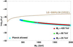
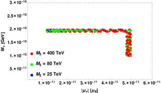
Figure 4: Left panel projects SI WIMP-nucleon cross section as a function $M_{R1}$, with dashed brown line of LZ-ZEPLIN upper limit Aalbers et al. (2022). Cyan data points satisfy Planck limit Aghanim et al. (2018) on relic abundance in $3\sigma$. Blue, green and red data points satisfy neutrino mass and magnetic moment for a specific set of values for fermion triplet and Yukawa, visible in the right panel.

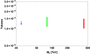
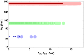
Figure 5: Left panel displays the suitable region for triplet mass and Yukawa to explain neutrino phenomenology. Right panel shows the allowed region for scalar mass splittings, thick (thin) bands correspond to $\delta_{\rm IR}(\delta_{\rm CR})$ respectively.

Using two specific benchmark values (shown in table. 2 and table. 3) which are favourable to explain both neutrino and dark matter aspects discussed so far, we project relic abundance scalar dark matter in Fig. 6.

Table 2: Set of benchmarks from the consistent parameter space.

	$M_{R1}$ [GeV]	$\delta$ [GeV]	$\delta_{\rm CR}$ [GeV]	$\delta_{\rm IR}$ [GeV]	$M_{\Sigma}$ [TeV]	Yukawa	$\sin\theta_{R}$
benchmark-1	$1472$	$101.69$	$9.03$	$0.35$	$420$	$10^{-4.89}$	$0.09$
benchmark-2	$628$	$36.40$	$4.38$	$3.45$	$80$	$10^{-4.85}$	$0.06$

Table 3: Neutrino and dark matter observables for the given benchmarks.

	$|\mu_{\nu}|$ [$\mu_{B}$]	$\mathcal{M}_{\nu}$ [GeV]	${\rm Log}^{[\sigma_{\rm SI}]}_{10}$ ${\rm cm}^{-2}$	$\Omega{\rm h}^{2}$
benchmark-1	$2.73\times 10^{-11}$	$1.99\times 10^{-10}$	$-47.78$	$0.123$
benchmark-2	$3.03\times 10^{-11}$	$1.92\times 10^{-10}$	$-47.04$	$0.119$

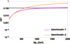
Figure 6: Relic density as a function of dark matter mass for the chosen benchmark of the favourable parameter space of table-2.

V.1 Constraints from neutrino oscillation parameters

More specific constraints on the Yukawa couplings can be obtained from the neutrino oscillation parameters. For this purpose, we consider the neutrino mixing matrix as the product of a tri-bimaximal (TBM) matrix with a rotation matrix $U_{13}$, given by

$$U_{\nu}=U_{\rm TBM}\cdot U_{13}=\left(\begin{array}[]{ccc}\cos\Theta&\sin\Theta&0\\ -\frac{\sin\Theta}{\sqrt{2}}&\frac{\cos\Theta}{\sqrt{2}}&\frac{1}{\sqrt{2}}\\ \frac{\sin\Theta}{\sqrt{2}}&-\frac{\cos\Theta}{\sqrt{2}}&\frac{1}{\sqrt{2}}\\ \end{array}\right)\cdot\left(\begin{array}[]{ccc}\cos\varphi&0&e^{-i\zeta}\sin\varphi\\ 0&1&0\\ -e^{i\zeta}\sin\varphi&0&\cos\varphi\\ \end{array}\right).$$ (27)

From eqns. 16,17, the matrices associated with neutrino magnetic moment and mass can be written in a compact form as

$$\mu_{\nu}=Y\cdot{\rm diag}(\Lambda_{1},\Lambda_{2},\Lambda_{3})\cdot Y^{T},$$

$$\mathcal{M}_{\nu}=Y\cdot{\rm diag}(\Lambda^{\prime}_{1},\Lambda^{\prime}_{2},\Lambda^{\prime}_{3})\cdot Y^{T},$$ (28)

where,

$$\Lambda_{k}=\frac{1}{8\pi^{2}}M_{\Sigma^{+}_{k}}\bigg{[}(1+\sin 2\theta_{C})\frac{1}{M^{2}_{C2}}\left(\ln\left[\frac{M^{2}_{C2}}{M^{2}_{\Sigma^{+}_{k}}}\right]-1\right)+(1-\sin 2\theta_{C})\frac{1}{M^{2}_{C1}}\left(\ln\left[\frac{M^{2}_{C1}}{M^{2}_{\Sigma^{+}_{k}}}\right]-1\right)\bigg{]},$$

$$\Lambda^{\prime}_{k}=\frac{1}{32\pi^{2}}M_{\Sigma^{+}_{k}}\Bigg{(}\Bigg{[}(1+\sin 2\theta_{C})\frac{M_{C2}^{2}}{M_{\Sigma^{+}_{k}}^{2}-M_{C2}^{2}}\ln\left(\frac{M^{2}_{\Sigma^{+}_{k}}}{M^{2}_{C2}}\right)+(1-\sin 2\theta_{C})\frac{M_{C1}^{2}}{M_{\Sigma^{+}_{k}}^{2}-M_{C1}^{2}}\ln\left(\frac{M^{2}_{\Sigma^{+}_{k}}}{M^{2}_{C1}}\right)\Bigg{]}$$

$$~{}~{}~{}~{}~{}~{}~{}~{}+\Bigg{[}(1+\sin 2\theta_{R})\frac{M_{R2}^{2}}{M_{\Sigma^{0}_{k}}^{2}-M_{R2}^{2}}\ln\left(\frac{M^{2}_{\Sigma^{0}_{k}}}{M^{2}_{R2}}\right)+(1-\sin 2\theta_{R})\frac{M_{R1}^{2}}{M_{\Sigma^{0}_{k}}^{2}-M_{R1}^{2}}\ln\left(\frac{M^{2}_{\Sigma^{0}_{k}}}{M^{2}_{R1}}\right)\Bigg{]}$$

$$~{}~{}~{}~{}~{}~{}~{}~{}-\Bigg{[}(1+\sin 2\theta_{I})\frac{M_{I2}^{2}}{M_{\Sigma^{0}_{k}}^{2}-M_{I2}^{2}}\ln\left(\frac{M^{2}_{\Sigma^{0}_{k}}}{M^{2}_{I2}}\right)+(1-\sin 2\theta_{I})\frac{M_{I1}^{2}}{M_{\Sigma^{0}_{k}}^{2}-M_{I1}^{2}}\ln\left(\frac{M^{2}_{\Sigma^{0}_{k}}}{M^{2}_{I1}}\right)\Bigg{]}\Bigg{)},$$

and

$$Y=\left(\begin{array}[]{ccc}Y_{e1}{}&~{}Y_{e2}{}&~{}Y_{e3}\\ Y_{\mu 1}{}&~{}Y_{\mu 2}{}&~{}Y_{\mu 3}\\ Y_{\tau 1}{}&~{}Y_{\tau 2}{}&~{}Y_{\tau 3}\\ \end{array}\right).$$ (30)

Diagonalizing the matrices in Eq. (28) using $U_{\nu}$, we obtain three unique solutions where the Yukawa couplings corresponding to different flavors become linearly dependent. The relations take the form

$$Y_{e1}=\left(\frac{\sqrt{2}\;\cos\Theta\,\cos\varphi\,}{\sin\Theta\,\cos\varphi-e^{-i\zeta}\sin\varphi}\right)Y_{\tau 1},\hskip 2.84544ptY_{e2}=-\frac{\sqrt{2}\;\sin\Theta\,}{\cos\Theta}Y_{\tau 2},\hskip 2.84544ptY_{e3}=\left(\frac{\sqrt{2}\;\cos\Theta\,\sin\varphi\,}{\sin\Theta\,\sin\varphi+e^{-i\zeta}\cos\varphi}\right)Y_{\tau 3},$$

$$Y_{\mu 1}=\left(\frac{e^{-i\zeta}\sin\varphi+\sin\Theta\,\cos\varphi}{e^{-i\zeta}\sin\varphi-\sin\Theta\,\cos\varphi}\right)Y_{\tau 1},\hskip 5.69046ptY_{\mu 2}=-Y_{\tau 2},\hskip 5.69046ptY_{\mu 3}=\left(\frac{e^{-i\zeta}\cos\varphi-\sin\Theta\,\sin\varphi}{e^{-i\zeta}\cos\varphi+\sin\Theta\,\sin\varphi}\right)Y_{\tau 3}.$$ (31)

Thus, the obtained diagonalized matrices associated with neutrino magnetic moment and mass in the basis of active neutrinos are Kashiwase and Suematsu (2013); Ho and Tandean (2013); Singirala (2017)

$$\mu^{D}_{\nu}=\left(\begin{array}[]{ccc}a_{1}~{}(Y^{2}_{\tau 1}\Lambda_{1})&0&0\\ 0&a_{2}~{}(Y^{2}_{\tau 2}\Lambda_{2})&0\\ 0&0&a_{3}~{}(Y^{2}_{\tau 3}\Lambda_{3})\\ \end{array}\right),\quad\mathcal{M}^{D}_{\nu}=\left(\begin{array}[]{ccc}a_{1}~{}(Y^{2}_{\tau 1}\Lambda^{\prime}_{1})&0&0\\ 0&a_{2}~{}(Y^{2}_{\tau 2}\Lambda^{\prime}_{2})&0\\ 0&0&a_{3}~{}(Y^{2}_{\tau 3}\Lambda^{\prime}_{3})\\ \end{array}\right),$$ (32)

where,

$$a_{1}=\frac{2e^{2i\zeta}}{(-e^{i\zeta}\cos\varphi\sin\Theta+\sin\varphi)^{2}},\hskip 5.69046pta_{2}=\frac{2}{\cos^{2}\Theta},\hskip 5.69046pta_{3}=\frac{2e^{-2i\zeta}}{(e^{-i\zeta}\cos\varphi+\sin\Theta\sin\varphi)^{2}}.$$ (33)

The matrix $U_{\nu}$ replicates the standard Pontecorvo-MakiNakagawa-Sakata (PMNS) matrix, where the mixing angles, $\Theta$ and $\varphi$ can be fixed using the observed neutrino oscillation parameters. Using the best-fit values on $\theta_{12},\theta_{13}$ and $\theta_{23}$ from Esteban et al. (2020), we get $\Theta=33.04^{\circ}$ and $\varphi=10.18^{\circ}$. Furthermore, we take $\zeta=180^{\circ}$ which falls within $1\sigma$ region of the observed value of CP phase $197^{+27}_{-24}$ Esteban et al. (2020). Substituting the above, we get,

$$|U_{\nu}|=\left(\begin{array}[]{ccc}0.8250{}&~{}0.5452{}&~{}0.1481\\ 0.2544{}&~{}0.5927{}&~{}0.7641\\ 0.5044{}&~{}0.5927{}&~{}0.6278\\ \end{array}\right),$$ (34)

which is consistent enough in comparison with the leptonic mixing matrix that can explain the observed mixing angles in $3\sigma$ region Esteban et al. (2020)

$$|U^{{\rm SK}-3\sigma}_{\rm PMNS}|=\left(\begin{array}[]{ccc}0.801\to 0.845{}&~{}0.513\to 0.579{}&~{}0.143\to 0.155\\ 0.234\to 0.500{}&~{}0.471\to 0.689{}&~{}0.637\to 0.776\\ 0.271\to 0.525{}&~{}0.477\to 0.694{}&~{}0.613\to 0.756\\ \end{array}\right).$$ (35)

Furthermore, the Yukawa matrix turns out to be

$$Y=\left(\begin{array}[]{ccc}1.6356~{}Y_{\tau 1}&-0.9197~{}Y_{\tau 2}&-0.2360~{}Y_{\tau 3}\\ -0.5044~{}Y_{\tau 1}&-Y_{\tau 2}&1.2170~{}Y_{\tau 3}\\ Y_{\tau 1}&Y_{\tau 2}&Y_{\tau 3}\\ \end{array}\right),$$ (36)

and the relevant coefficients in the diagonal matrices of eqn. 32 become $a_{1}=3.930$, $a_{2}=2.846$ and $a_{3}=2.537$.

To illustrate, we consider all the three generations of heavy fermion triplets to be degenerate in mass i.e., $m_{\Sigma}\sim 420$ TeV and scan the DM consistent parameter space to extract the constraints on Yukawa. In Fig. 7, we project the allowed region of Yukawa (shown as cyan, magenta and orange data points) that satisfies the required bound on mass squared differences Esteban et al. (2020) in $3\sigma$ (blue and black dashed lines) and also cosmological bound on sum of active neutrino masses i.e., $0.058\leq(m_{1}+m_{2}+m_{3})\leq 0.12$ eV (normal hierarchy) Roy Choudhury and Choubey (2018) represented as green vertical lines. To mention, this projected parameter space is consistent with neutrino magnetic moment in a wide range of values, i.e., $3\times 10^{-12}$ to $7\times 10^{-10}$ (in units of $\mu_{B}$), which is the regime where all the experiments have provided the bounds (to be discussed in the next section).

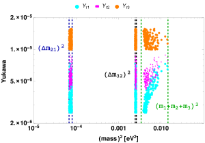
Figure 7: Allowed region of Yukawa (colored data points), satisfying the $3\sigma$ limit on mass squared differences Esteban et al. (2020) and cosmological bounds on sum of active neutrino masses Roy Choudhury and Choubey (2018) (colored vertical lines).

VI Implications

In the experimental perspective, non-zero neutrino magnetic moment of solar neutrinos can provide explanation for the excess in electron recoil events at XENON1T collaboration Aprile et al. (2020a). In other words, the neutrino transition magnetic moment can provide additional contribution to the neutrino-electron scattering process. In this section, we utilize non-zero transition neutrino magnetic moment to explain the excess in electron recoil events.

In the presence of magnetic moment, the total differential cross section can be written as Giunti et al. (2016)

$$\left(\frac{d\sigma}{dT_{e}}\right)_{\rm TOT}=\left(\frac{d\sigma}{dT_{e}}\right)_{\rm SM}+\left(\frac{d\sigma}{dT_{e}}\right)_{\rm EM},$$ (37)

where $T_{e}$ is the electron recoil energy. The first contribution in eq. 37 is due to standard weak interactions, given by

$$\left(\frac{d\sigma}{dT_{e}}\right)_{\rm SM}=\frac{G_{F}^{2}m_{e}}{2\pi}\left[(g_{V}+g_{A})^{2}+\left(1-\frac{T_{e}}{E_{\nu}}\right)^{2}(g_{V}-g_{A})^{2}+\left(\frac{m_{e}T_{e}}{E_{\nu}^{2}}\right)(g^{2}_{A}-g^{2}_{V})\right].$$ (38)

In the above, $G_{F}$ stands for the Fermi constant and

$$g_{V}=2\sin^{2}\theta_{W}+\frac{1}{2},~{}~{}g_{A}=1/2~{}~{}{\rm for}~{}~{}\nu_{e},$$

$$g_{V}=2\sin^{2}\theta_{W}-\frac{1}{2},~{}~{}g_{A}=-1/2~{}~{}{\rm for}~{}~{}\nu_{\mu},\nu_{\tau}.$$ (39)

The second contribution comes from the effective electromagnetic vertex of the neutrinos, i.e., magnetic moment contribution, which is expressed as

$$\left(\frac{d\sigma}{dT_{e}}\right)_{\rm EM}=\frac{\pi\alpha^{2}}{m^{2}_{e}}\left(\frac{1}{T_{e}}-\frac{1}{E_{\nu}}\right)\left(\frac{\mu_{\nu_{e\mu}}}{\mu_{B}}\right)^{2},$$ (40)

where, $\alpha$ is the electromagnetic coupling, $E_{\nu}$ is the initial neutrino energy, $\mu_{\nu_{e\mu}}$ is the neutrino magnetic moment and $\mu_{B}$ is the Bohr magneton. For high $T_{e}$ value, weak cross-section dominates and for low $T_{e}$ value, the electromagnetic cross-section dominates and hence, we search for the signature of neutrino magnetic moment in the low energy region. For simplicity, we take one transition magnetic moment $\mu_{{\nu}_{e\mu}}$ to explain the XENON1T excess. The differential event rate to estimate the XENON1T signal is given by

$$\frac{dN}{dT_{r}}=n_{\rm te}\times\int^{E^{\rm max}_{\nu}}_{E^{\rm min}_{\nu}}dE_{\nu}\int_{T_{\rm th}}^{T_{\rm max}}dT_{e}\left(\frac{d\sigma^{\nu_{e}e}}{dT_{e}}P_{ee}+\cos^{2}\theta_{23}\frac{d\sigma^{\nu_{\mu}e}}{dT_{e}}P_{e\mu}\right)\times\frac{d\phi_{s}}{dE_{\nu}}\times\varepsilon(T_{e})\times G(T_{e},T_{r}).$$ (41)

In the above, $\varepsilon(T_{e})$ denotes the efficiency of detector Aprile et al. (2020a), $n_{te}$ is the count of number of target electrons in the fiducial volume of one ton Xenon Aprile et al. (2020b), $d\phi_{s}/dE_{\nu}$ represents the solar neutrino flux spectrum Bahcall and Pena-Garay (2004), and the function $G(T_{e},T_{r})$ reflects the normalised Gaussian smearing function that takes into account the detector’s limited energy resolution Aprile et al. (2020a). The limits $T_{\rm th}=1$ KeV and $T_{\rm max}=30$ KeV stand for the threshold and maximum recoil energy of detector respectively. The extremes of neutrino energy for the integral are given by $E^{\rm max}_{\nu}=420$ KeV and $E^{\rm min}_{\nu}=[T+(2m_{e}T+T^{2})^{\frac{1}{2}}]/2$ Babu et al. (2020). The survival probability can be expressed as

$$P_{ee}=\sin^{4}\theta_{13}+\frac{1}{2}\cos^{4}\theta_{13}(1+\cos 2\theta^{m}_{12}+\cos 2\theta_{12})\;.$$ (42)

And the disappearance probability can be taken as $P_{e\mu/\tau}$ = $1-P_{ee}$ Lopes and Turck-Chièze (2013); Zyla et al. (2020). The oscillation parameters are taken from Esteban et al. (2020). In Fig. 8, we project the event rate as a function of recoil energy $T_{r}$, for two set of values for magnetic moment, i.e., $\mu_{\nu_{e\mu}}=2.6\times 10^{-11}\mu_{B}$ and $3.2\times 10^{-11}\mu_{B}$ (red curves). Adding with the background (green curve), we are able to meet the observed recoil event excess in the low energy region near $2.5$ KeV as of XENON1T experiment Aprile et al. (2020a).

In Fig. 9, we project neutrino magnetic moment as a function of dark matter mass, choosing specific set of values assigned to triplet fermion. As seen earlier in the left panel of Fig. 4, a specific range of dark matter mass is favoured with the scale of triplet mass. It is transparent that the model parameters are able to provide neutrino magnetic moment in the range $10^{-12}\mu_{B}$ to $10^{-10}\mu_{B}$, sensitive to the upper limits of Super-K Liu et al. (2004), TEXONO Wong et al. (2007), Borexino Agostini et al. (2017), XENON1T Aprile et al. (2020a), XENONnT Aprile et al. (2022) and white dwarfs Miller Bertolami (2014) (colored horizontal lines). Thus, from all the above discussions made, it is evident that this simple framework can provide a consistent phenomenological platform for a correlative study of neutrino magnetic moment (especially), mass and dark matter physics.

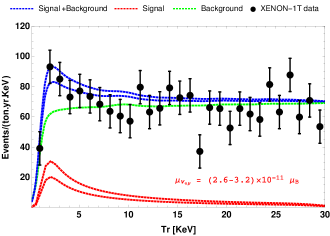
Figure 8: Excess recoil events (blue) to match XENON1T Aprile et al. (2020a) (black) through the signal from transition neutrino magnetic moment $\mu_{\nu_{e\mu}}=2.6\times 10^{-11}\mu_{B}$ and $3.2\times 10^{-11}\mu_{B}$ (in red) along with background (green).

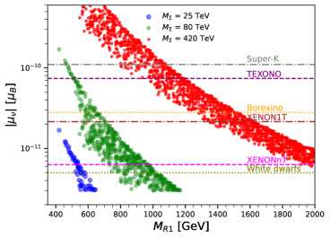
Figure 9: Allowed region of neutrino magnetic moment with the mass spectrum of dark matter and fermion triplet. Horizontal colored lines stand for the upper bounds of XENON1T (average value of suggested range in Aprile et al. (2020a)), XENONnT Aprile et al. (2022), Borexino Agostini et al. (2017), TEXONO Wong et al. (2007), Super-K Liu et al. (2004) and white dwarfs Miller Bertolami (2014).

VII Concluding remarks

The primary aim is to address neutrino mass, magnetic moment and dark matter phenomenology in a common framework. For this purpose, we have extended the standard model with three vector-like fermion triplets and two inert scalar doublets to realize Type-III radiative scenario. A pair of charged scalars help in obtaining neutrino magnetic moment, all charged and neutral scalars come up in getting light neutrino mass at one-loop level. All the inert scalars participate in annihilation and co-annihilation channels to provide total dark matter relic density of the Universe, consistent with Planck satellite data and also provide a suitable cross section with nucleon, sensitive to LZ-ZEPLIN upper limit. The lightest dark matter mass is scanned upto $2$ TeV while the fermion triplet mass is taken with larger values, i.e., few hundred TeV. Choosing Yukawa of the order $10^{-5}$, we have obtained light neutrino mass in sub-eV scale and also transition magnetic moment $\sim 10^{-11}$ $\mu_{B}$, to successfully explain the excess electron recoil events at low energy scale reported by XENON1T experiment. Finally, we have also demonstrated with a plot that the model is able to provide neutrino magnetic moment in a wide range ($10^{-12}\mu_{B}$ to $10^{-10}\mu_{B}$), in the same ball park of Borexino, Super-K, TEXONO, XENONnT and white dwarfs. Overall, this simple model provides a suitable platform to study neutrino phenomenology, especially the neutrino magnetic moment and also dark matter aspects.

References

• Bilenky (1999) S. M. Bilenky, in 1999 European School of High-Energy Physics (1999), pp. 187–217, eprint hep-ph/0001311.
• Mohapatra and Senjanovic (1980) R. N. Mohapatra and G. Senjanovic, Phys. Rev. Lett. 44, 912 (1980).
• Schechter and Valle (1980) J. Schechter and J. W. F. Valle, Phys. Rev. D 22, 2227 (1980).
• Babu and Mohapatra (1993) K. Babu and R. Mohapatra, Phys. Rev. Lett. 70, 2845 (1993), eprint hep-ph/9209215.
• Hosaka et al. (2006) J. Hosaka et al. (Super-Kamiokande), Phys. Rev. D 73, 112001 (2006), eprint hep-ex/0508053.
• Ahmad et al. (2002) Q. R. Ahmad et al. (SNO), Phys. Rev. Lett. 89, 011301 (2002), eprint nucl-ex/0204008.
• Abe et al. (2016) K. Abe et al. (Super-Kamiokande), Phys. Rev. D 94, 052010 (2016), eprint 1606.07538.
• Abe et al. (2019) K. Abe et al. (T2K), Phys. Rev. D 99, 071103 (2019), eprint 1902.06529.
• An et al. (2012) F. P. An et al. (Daya Bay), Phys. Rev. Lett. 108, 171803 (2012), eprint 1203.1669.
• Abe et al. (2012) Y. Abe et al. (Double Chooz), Phys. Rev. Lett. 108, 131801 (2012), eprint 1112.6353.
• Zwicky (1937) F. Zwicky, Astrophys. J. 86, 217 (1937).
• Zwicky (1933) F. Zwicky, Phys. Rev. 43, 147 (1933), URL https://link.aps.org/doi/10.1103/PhysRev.43.147.
• Bertone et al. (2005) G. Bertone, D. Hooper, and J. Silk, Phys. Rept. 405, 279 (2005), eprint hep-ph/0404175.
• Mambrini et al. (2015) Y. Mambrini, N. Nagata, K. A. Olive, J. Quevillon, and J. Zheng, Phys. Rev. D 91, 095010 (2015), eprint 1502.06929.
• Sakharov (1991) A. Sakharov, Sov. Phys. Usp. 34, 392 (1991).
• Kolb and Wolfram (1980) E. W. Kolb and S. Wolfram, Nucl. Phys. B 172, 224 (1980), [Erratum: Nucl.Phys.B 195, 542 (1982)].
• Fukugita and Yanagida (1986) M. Fukugita and T. Yanagida, Phys. Lett. B 174, 45 (1986).
• Fritzsch and Minkowski (1975) H. Fritzsch and P. Minkowski, Annals Phys. 93, 193 (1975).
• Bifani et al. (2019) S. Bifani, S. Descotes-Genon, A. Romero Vidal, and M.-H. Schune, J. Phys. G 46, 023001 (2019), eprint 1809.06229.
• Aprile et al. (2020a) E. Aprile et al. (XENON), Phys. Rev. D 102, 072004 (2020a), eprint 2006.09721.
• Aprile et al. (2022) E. Aprile et al. (XENON), Phys. Rev. Lett. 129, 161805 (2022), eprint 2207.11330.
• Miranda et al. (2020) O. G. Miranda, D. K. Papoulias, M. Tórtola, and J. W. F. Valle, Phys. Lett. B 808, 135685 (2020), eprint 2007.01765.
• Li and Xia (2022) Y.-F. Li and S.-y. Xia, Phys. Rev. D 106, 095022 (2022), eprint 2203.16525.
• Miranda et al. (2021) O. G. Miranda, D. K. Papoulias, O. Sanders, M. Tórtola, and J. W. F. Valle, JHEP 12, 191 (2021), eprint 2109.09545.
• Babu et al. (2021) K. S. Babu, S. Jana, M. Lindner, and V. P. K, JHEP 10, 240 (2021), eprint 2104.03291.
• Brdar et al. (2021) V. Brdar, A. Greljo, J. Kopp, and T. Opferkuch, JCAP 01, 039 (2021), eprint 2007.15563.
• Khan (2023a) A. N. Khan, Phys. Lett. B 837, 137650 (2023a), eprint 2208.02144.
• Khan (2023b) A. N. Khan, Nucl. Phys. B 986, 116064 (2023b), eprint 2201.10578.
• Jeong et al. (2021) J. Jeong, J. E. Kim, and S. Youn, Int. J. Mod. Phys. A 36, 2150182 (2021), eprint 2105.01842.
• Alok et al. (2023) A. K. Alok, N. R. Singh Chundawat, and A. Mandal, Phys. Lett. B 839, 137791 (2023), eprint 2207.13034.
• Dror et al. (2021) J. A. Dror, G. Elor, R. McGehee, and T.-T. Yu, Phys. Rev. D 103, 035001 (2021), [Erratum: Phys.Rev.D 105, 119903 (2022)], eprint 2011.01940.
• Agostini et al. (2017) M. Agostini et al. (Borexino), Phys. Rev. D 96, 091103 (2017), eprint 1707.09355.
• Wong et al. (2007) H. T. Wong et al. (TEXONO), Phys. Rev. D 75, 012001 (2007), eprint hep-ex/0605006.
• Liu et al. (2004) D. W. Liu et al. (Super-Kamiokande), Phys. Rev. Lett. 93, 021802 (2004), eprint hep-ex/0402015.
• Miller Bertolami (2014) M. M. Miller Bertolami, Astron. Astrophys. 562, A123 (2014), eprint 1407.1404.
• Keus et al. (2014a) V. Keus, S. F. King, S. Moretti, and D. Sokolowska, JHEP 11, 016 (2014a), eprint 1407.7859.
• Keus et al. (2014b) V. Keus, S. F. King, and S. Moretti, Phys. Rev. D 90, 075015 (2014b), eprint 1408.0796.
• Cao et al. (2007) Q.-H. Cao, E. Ma, and G. Rajasekaran, Phys. Rev. D 76, 095011 (2007), eprint 0708.2939.
• Lundstrom et al. (2009) E. Lundstrom, M. Gustafsson, and J. Edsjo, Phys. Rev. D 79, 035013 (2009), eprint 0810.3924.
• Cirelli et al. (2006) M. Cirelli, N. Fornengo, and A. Strumia, Nucl. Phys. B 753, 178 (2006), eprint hep-ph/0512090.
• Xing and Zhou (2011) Z.-z. Xing and S. Zhou, Neutrinos in particle physics, astronomy and cosmology (2011), ISBN 978-3-642-17559-6, 978-7-308-08024-8.
• Babu et al. (2020) K. S. Babu, S. Jana, and M. Lindner, JHEP 10, 040 (2020), eprint 2007.04291.
• Chen et al. (2021) S.-L. Chen, A. Dutta Banik, and Z.-K. Liu, Nucl. Phys. B 966, 115394 (2021), eprint 2011.13551.
• Lineros and Pierre (2020) R. A. Lineros and M. Pierre, JHEP 21, 072 (2020), eprint 2011.08195.
• Ávila et al. (2020) I. M. Ávila, V. De Romeri, L. Duarte, and J. W. F. Valle, Eur. Phys. J. C 80, 908 (2020), eprint 1910.08422.
• Lopez Honorez et al. (2007) L. Lopez Honorez, E. Nezri, J. F. Oliver, and M. H. G. Tytgat, JCAP 02, 028 (2007), eprint hep-ph/0612275.
• Barbieri et al. (2006) R. Barbieri, L. J. Hall, and V. S. Rychkov, Phys. Rev. D 74, 015007 (2006), eprint hep-ph/0603188.
• Dolle and Su (2009) E. M. Dolle and S. Su, Phys. Rev. D 80, 055012 (2009), eprint 0906.1609.
• Ellis et al. (2000) J. R. Ellis, A. Ferstl, and K. A. Olive, Phys. Lett. B 481, 304 (2000), eprint hep-ph/0001005.
• Semenov (1996) A. V. Semenov (1996), eprint hep-ph/9608488.
• Pukhov et al. (1999) A. Pukhov, E. Boos, M. Dubinin, V. Edneral, V. Ilyin, D. Kovalenko, A. Kryukov, V. Savrin, S. Shichanin, and A. Semenov (1999), eprint hep-ph/9908288.
• Belanger et al. (2007) G. Belanger, F. Boudjema, A. Pukhov, and A. Semenov, Comput. Phys. Commun. 176, 367 (2007), eprint hep-ph/0607059.
• Belanger et al. (2009) G. Belanger, F. Boudjema, A. Pukhov, and A. Semenov, Comput. Phys. Commun. 180, 747 (2009), eprint 0803.2360.
• Aghanim et al. (2018) N. Aghanim et al. (Planck) (2018), eprint 1807.06209.
• Aalbers et al. (2022) J. Aalbers et al. (LZ) (2022), eprint 2207.03764.
• Kashiwase and Suematsu (2013) S. Kashiwase and D. Suematsu, Eur. Phys. J. C 73, 2484 (2013), eprint 1301.2087.
• Ho and Tandean (2013) S.-Y. Ho and J. Tandean, Phys. Rev. D 87, 095015 (2013), eprint 1303.5700.
• Singirala (2017) S. Singirala, Chin. Phys. C 41, 043102 (2017), eprint 1607.03309.
• Esteban et al. (2020) I. Esteban, M. C. Gonzalez-Garcia, M. Maltoni, T. Schwetz, and A. Zhou, JHEP 09, 178 (2020), eprint 2007.14792.
• Roy Choudhury and Choubey (2018) S. Roy Choudhury and S. Choubey, JCAP 09, 017 (2018), eprint 1806.10832.
• Giunti et al. (2016) C. Giunti, K. A. Kouzakov, Y.-F. Li, A. V. Lokhov, A. I. Studenikin, and S. Zhou, Annalen Phys. 528, 198 (2016), eprint 1506.05387.
• Aprile et al. (2020b) E. Aprile et al. (XENON), Eur. Phys. J. C 80, 785 (2020b), eprint 2003.03825.
• Bahcall and Pena-Garay (2004) J. N. Bahcall and C. Pena-Garay, New J. Phys. 6, 63 (2004), eprint hep-ph/0404061.
• Lopes and Turck-Chièze (2013) I. Lopes and S. Turck-Chièze, Astrophys. J. 765, 14 (2013), eprint 1302.2791.
• Zyla et al. (2020) P. A. Zyla et al. (Particle Data Group), PTEP 2020, 083C01 (2020).