The Entanglement of Elastic and Inelastic Scattering

Abstract

The entanglement properties of systems in which elastic and inelastic reactions occur in projectile-target interactions is studied. A new measure of entanglement, the scattering entropy, based on the unitarity of the $S-$matrix (probability conservation), is suggested. Using simple models for both low- and high-energy interactions, the amount of entanglement is found to track with the strength of the inelastic interaction. The familiar example of the classical “black disk”, total absorption, model is found to correspond to maximum entanglement. An analysis of high-energy $pp$ scattering data shows that entanglement is near maximum for lab energies greater than about 1 GeV, showing that the total absorption model is a reasonable starting point for understanding the data.

I Introduction

The implications of entanglement in quantum mechanics and quantum field theory have recently been studied in many papers. For a long list of recent references see Ref. Ehlers (2022). This new interest has been stimulated by the connection with quantum computing. Work related to hadron, QCD and EIC physics appears in Refs. Kharzeev and Levin (2017); Feal et al. (2019); Gotsman and Levin (2020); Hentschinski et al. (2022); Wang and Chen (2015); Beane and Ehlers (2019). The entanglement properties of nucleon-nucleon scattering and nucleon-nucleus elastic scattering are discussed in Refs. Beane et al. (2019); Liu et al. (2023); Miller (2023); Bai (2023); Bai and Ren (2022). The connections between entanglement and nuclear structure are presented in Johnson and Gorton (2023); Kruppa et al. (2021, 2022); Robin et al. (2021); Pazy (2023); Tichai et al. (2022); Gu et al. (2023); Bulgac (2022); Bulgac et al. (2023). There is also a possible deep connection between entanglement and underlying symmetries of the Standard Model Cervera-Lierta et al. (2017); Beane et al. (2019); Liu et al. (2023); Bai (2023); Miller (2023).

The present paper is concerned with situations in which a projectile can excite a target. One of the challenges in studying entropy and entanglement for scattering is the need to develop proper definitions for the necessary infinite dimensional Hilbert space. This is done here using the requirements of unitarity.

A special and somewhat ubiquitous case is the scattering of a particle from a totally absorbing “black disk” of radius $R$ Kovchegov and Levin (2013); Frauenfelder and Henley (1991); Gottfried (2018). This situation approximately occurs in low-energy $\alpha$-nucleus scattering, and in high-energy proton-proton scattering. In the total absorption limit, following the requirement of unitarity of the $S$-matrix, the elastic $\sigma_{\rm el}$ and inelastic $\sigma_{\rm inel}$ cross sections are equal. The inelastic cross section cross section, is $\pi R^{2}$, so that the total cross section is 2$\pi R^{2}$, twice the geometric cross section. I will argue that when $\sigma_{\rm el}=\sigma_{\rm inel}$ the entanglement entropy is maximized.

II Low-energy projectile-target scattering and a new measure of entropy

Consider projectile-target scattering at energies sufficient low so that there is only $s$-wave scattering. Furthermore, the model definition is that there is only inelastic scattering to a single excited state, $X$. I consider examples in which the inelastic scattering ranges from relatively small, corresponding, for example, to neutron-nucleus scattering, to relatively large, corresponding to alpha-nucleus scattering. Another example, discussed below, is nucleon-nucleon scattering in which interactions cause either the target or projectile to be in an excited state.

The initial state is a product of a plane wave state and the target ground state, $G$. As a product state there is no entanglement. Interactions occur such that after the scattering event the projectile-target wave function is given by

$$|\Psi\rangle=|u_{1}\rangle\otimes|G\rangle+|u_{2}\rangle\otimes|X\rangle,$$ (1)

where $|u_{1}\rangle$ represents a projectile with energy corresponding to elastic scattering and $|u_{2}\rangle$ represents a projectile with an energy corresponding to inelastic scattering. Measurement of the energy of the projectile determines whether or not the nucleus is in its ground or excited state. Thus the state represented by Eq. (1) is an entangled state. The next step is to work out a way to calculate entanglement properties. The wave function, $|\Psi\rangle$ is almost of the form of the Schmidt decomposition in which the different coefficients represent probability amplitudes. Here the wave functions are in the continuum, so that discrete normalization conventions are not applicable. It seems necessary to develop a new method to compute entropy.

The procedure is to use an exactly soluble model  Kamal and Kreuzer (1970) to illustrate and develop the necessary formalism. I argue below that the formalism is more general than the model. In this model the interactions are represented by delta-shell interactions Gottfried (2018) that can be thought of as approximating projectile-target interactions at the surface of the target. Then the radial wave functions $u_{1,2}(r)$ satisfy the coupled-channels equations:

$$d^{2}u_{1}/dr^{2}+[k^{2}-V_{1}\delta(r-a)]u_{1}=V_{12}\delta(r-a)u_{2},$$ (2)

$$d^{2}u_{2}/dr^{2}+[k^{2}-\Delta^{2}-V_{2}\delta(r-a)]u_{1}=V_{21}\delta(r-a)u_{2}.$$ (3)

Hermiticity demands $V_{12}=V_{21}$ and calculations are limited to the case $V_{1}\neq 0,\,V_{12}\neq 0,V_{2}=0$ to gain analytic insight. The parameter $\Delta$ is proportional to the energy difference between the excited and ground states. The solution of Eq. (2) for $u_{1}$ is expressed in terms of the free-particle Green’s function $g_{1}(r,r^{\prime})$ as

$$u_{1}(r)={\sin{kr}\over k}+V_{1}g_{1}(r,a)u_{1}(a)+V_{12}g_{1}(r,a)u_{2}(a),$$

(4)

with

$$g_{1}(r,r^{\prime})=-(1/k)\sin{kr_{<}}e^{ikr_{>}},$$ (5)

$r_{<}(r_{>})$ is the smaller (larger) of $(r,r^{\prime})$. The solution of Eq. (3) for $u_{2}$ is given by

$$u_{2}(r)=V_{12}g_{2}(r,a)u_{1}(a)$$ (6)

with

$$g_{2}(r,r^{\prime})=-(1/k_{2})\sin{k_{2}r_{<}}e^{ik_{2}r_{>}},$$ (7)

where $k_{2}\equiv\sqrt{k^{2}-\Delta^{2}}$. The results for $u_{1,2}(r)$ express the condition that the initial state is a plane wave incident on the ground state of the target nucleus. The use of Eq. (6) in Eq. (4) leads to the result

$$u_{1}(r)=(1/k)\sin{kr}+T_{11}e^{ikr}$$ (8)

for $r>a$, with the $T$-matrix element given by

$$T_{11}={({\sin{ka}\over k})^{2}[V_{1}+V_{12}^{2}g_{2}(a,a)]\over 1-[V_{1}+V_{12}^{2}g_{2}(a,a)]g_{1}(a,a)}.$$ (9)

The relation between $T_{11}$ and the complex-valued scattering phase shift, $\delta_{0}$, is given by

$$T_{11}={e^{2i\delta_{0}}-1\over 2ik}.$$ (10)

Similarly

$$u_{2}(r)=T_{12}e^{ik_{2}r},$$ (11)

with

$$T_{12}={V_{12}({\sin{ka}\over k})({\sin{k_{2}a}\over k_{2}})\over 1-[V_{1}+V_{12}^{2}g_{2}(a,a)]g_{1}(a,a)}.$$ (12)

Next, turn to the entanglement properties of the model. The textbook definition is the entanglement entropy, the von Neumann entropy, given by $S=-{\rm Tr}[\rho\log_{2}\rho],$ where $\rho$ is the one-body density matrix. This is typically evaluated by diagonalizing $\rho$ in a discrete basis. Here continuum wave functions, normalized as delta functions, are used. So there is a need to obtain an appropriate definition of probability. This is done through the optical theorem, an expression of the unitarily of the $S$-matrix:

$$\sigma_{tot}={4\pi\over k_{1}}{\rm Im}[T_{11}].$$ (13)

The left-hand side is sum of the elastic and inelastic scattering cross sections, integrated over all angles. The result for the present model is expressed as

$$1={k_{1}|T_{11}|^{2}+k_{2}|T_{12}|^{2}\over{\rm Im}[T_{11}]},$$ (14)

a relation that can be checked using the expressions for $T_{11}$ and $T_{12}$. The Eq. (14) leads to a natural definition of probabilities based on the number of counts detected at an asymptoticaly located detector. The ground state probability $P_{G}$ is given by

$$P_{G}={k_{1}|T_{11}|^{2}\over{\rm Im}[T_{11}]}$$ (15)

and the excited state probability $P_{X}$ is given by

$$P_{X}={k_{2}|T_{12}|^{2}\over{\rm Im}[T_{11}]},$$ (16)

and via Eq. (14): $P_{G}+P_{X}=1$.

Therefore, one may define the projectile-target $(pT)$ entanglement entropy $S_{pT}$ of the final state as

$$S_{pT}=-P_{G}\ln_{2}P_{G}-P_{X}\ln_{2}P_{X}.$$ (17)

This entanglement entropy, termed the scattering entropy, is minimized if either of $P_{G}$ or $P_{X}$ vanishes. In that case the final scattering state is a simple tensor product. The scattering entropy is maximized at $S_{pT}=1$ when $P_{G}=P_{X}.$ Note also that Eq. (10) shows that $T_{11}$ is periodic in $k$, vanishing whenever $k=n\pi$.

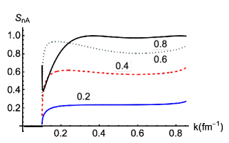
Figure 1: $S_{nA}$ as a function of $k=k_{1}$ for the four different values of $V_{12}/V$ shown in the figure.

Fig. 1 shows $S_{pT}$ for parameters $a=3.5\,\rm fm,V_{1}=0.25\,\rm fm^{-1}$ for different ratios $V_{12}/V_{1}$ as a function of $k$ the incident momentum. The parameter $\Delta=0.1$ fm^-1. The situation of $V_{12}/V_{1}=0.2$ is similar to that of neutron-nucleus interactions in which the inelastic scattering is relatively small. The stronger absorption situation of $V_{12}/V_{1}=1$ is similar to that of alpha-nucleus interactions in which the inelastic scattering is large.

For values of $k<\Delta$ the entanglement entropy vanishes because the target cannot be excited. For higher values the scattering entropy is at its maximum value when $V_{12}/V_{1}=1$. This result can be understood directly from Eq. (15) and Eq. (16). These quantities are approximately equal if $V/(ka)\ll 1$ and $k\gg\Delta$. This result is similar to that of the total absorption model in which the elastic and inelastic cross sections are the same. But here there is only one phase shift. The unusual cusp-like near-threshold behavior for the case when $V_{12}/V_{1}=1$ arises from the non-analytic square root behavior of $k_{2}$ combined with the increasing importance of the second term in the numerator of Eq. (9).

The key lesson of Fig. 1 is that entanglement entropy, as measured by the scattering entropy, increases as the tendency for inelastic scattering increases.

III High energy scattering in a two-channel model

The scattering wave function $|\Psi\rangle$ is given again by Eq. (1). In the high energy limit the wave number $k$ is large compared to the inverse size of the system and large compared to the energy difference between the ground and excited states represented by $\Delta$. Thus $\Delta$ is neglected in solving the relevant wave equations, but kept as very small, but non-zero, to maintain the entanglement property that measuring energy of the projectile in the final state determines whether or not the target is in the ground state.

The coupled-channel equations for high-energy scattering are then given by

$$\nabla^{2}\psi_{1}+(k^{2}-V)\psi_{1}=U\psi_{2}$$ (18)

$$\nabla^{2}\psi_{2}+(k^{2}-V)\psi_{2}=U\psi_{1}$$ (19)

The implementation of the eikonal or short-wavelength approximation is made by using $\psi_{1,2}({\bf r})=e^{ikz}\phi_{1,2}({\bf b},z)$ in which the direction of the beam is denoted as $\hat{z}$ and the direction transverse to that by ${\bf b}$. The procedure Glauber (1959) is to use these in the coupled-channel equations and with large $k$ neglect the terms $\nabla^{2}\phi_{1,2}$. This approximation is valid under two conditions Glauber (1959): (i) the short-wavelength limit that $1/k$ is less than any distance scale in the problem, and (ii) $(V,U)/k^{2}\ll 1$ to prevent back-scattering. Then the coupled-channel equations become

$$2ik{\partial\phi_{1}\over\partial z}-V\phi_{1}=U\phi_{2}$$ (20)

$$2ik{\partial\phi_{2}\over\partial z}-V\phi_{2}=U\phi_{1}.$$ (21)

Let $\phi\equiv\phi_{1}+\phi_{2}$ and $\chi\equiv\phi_{1}-\phi_{2}$. Adding the two equations gives

$$2ik{\partial\phi\over\partial z}=(U+V)\phi,$$ (22)

and subtracting the two gives

$$2ik{\partial\chi\over\partial z}=(V-U)\phi$$ (23)

with solutions

$$\phi({\bf b},z)=\exp[{{-i\over 2k}\int_{-\infty}^{z}dz^{\prime}(V({\bf b},z^{\prime})+U({\bf b},z^{\prime}))}$$ (24)

$$\chi({\bf b},z)=\exp[{{-i\over 2k}\int_{-\infty}^{z}dz^{\prime}(V({\bf b},z^{\prime})-U({\bf b},z^{\prime}))}.$$ (25)

The two-component scattering amplitude is given by

$$\hat{f}({\bf k}^{\prime},{\bf k})={-1\over 4\pi}\int d^{3}re^{-i{\bf k}^{\prime}\cdot{\bf b}}\begin{bmatrix}V&U\\ U&V\end{bmatrix}\begin{bmatrix}\phi_{1}\\ \phi_{2}\end{bmatrix},$$ (26)

with the upper row of $\hat{f}$, $f_{G}$, corresponding to elastic scattering and the lower row, $f_{X}$, to inelastic scattering. Then evaluation leads to the results

$$f_{G}({\bf k}^{\prime},{\bf k})={ik\over 2\pi}\int d^{2}be^{-i{\bf k}^{\prime}\cdot{\bf b}}(1-e^{-i\delta_{V}({\bf b})}\cos\delta_{U}({\bf b}))$$ (27)

$$f_{X}({\bf k}^{\prime},{\bf k})={-k\over 2\pi}\int d^{2}be^{-i{\bf k}^{\prime}\cdot{\bf b}}e^{-i\delta_{V}({\bf b})}\sin\delta_{U}({\bf b}),$$ (28)

where

$$\delta_{V}\equiv{1\over 2k}\int_{-\infty}^{\infty}dz^{\prime}V({\bf b},z^{\prime}),\,\delta_{U}\equiv{1\over 2k}\int_{-\infty}^{\infty}dz^{\prime}U({\bf b},z^{\prime}).$$ (29)

The evaluation of entanglement entropy requires an understanding of unitarity. The statement of unitarity via the optical theorem is

$$\sigma_{Tot}=\int d\Omega(|f_{G}|^{2}+|f_{X}|^{2})={4\pi\over k}\rm{Im}[f_{G}({\bf k}^{\prime},{\bf k})],$$ (30)

a relationship that must be checked within the current model. Taking the imaginary part of Eq. (27) yields

$${\rm Im}[f_{G}({\bf k},{\bf k})]={k\over 2\pi}\int d^{2}b(1-\cos{\delta_{V}({\bf b})}\cos\delta_{U}({\bf b})).$$ (31)

The evaluation of the angular integrals of $|f_{G,X}|^{2}$ may be done using an approximation, valid when the eikonal approximation is valid, namely

$$\int d\Omega e^{i{\bf k}^{\prime}\cdot({\bf b}-{\bf b}^{\prime})}\approx 2\pi{1\over k^{2}b}\delta(b-b^{\prime}).$$ (32)

Using this leads to the results

$$\int d\Omega|f_{G}({\bf k}^{\prime},{\bf k})|^{2}=\int d^{2}b(1-2\cos\delta_{V}\cos\delta_{U}+\cos^{2}\delta_{U})$$

$$\int d\Omega|f_{X}({\bf k}^{\prime},{\bf k})|^{2}=\int d^{2}b\sin^{2}\delta_{U},$$ (33)

so that the validity of Eq. (30) is maintained. Therefore we may again define the eikonal probability, $P^{e}_{G,X},$ as

$$P_{G}^{e}={\int d^{2}b(1-2\cos\delta_{V}(b)\cos\delta_{U}(b)+\cos^{2}\delta_{U}(b))\over 2\int d^{2}b(1-\cos{\delta_{V}(b)}\cos\delta_{U}(b))}$$ (34)

$$P_{X}^{e}={\int d^{2}b\sin^{2}\delta_{U}(b)\over\int d^{2}b2(1-\cos{\delta_{V}(b)}\cos\delta_{U}(b))},$$ (35)

and

$$S^{e}=-P_{G}^{e}\ln_{2}P^{e}_{G}-P^{e}_{X}\ln_{2}P^{e}_{X}.$$ (36)

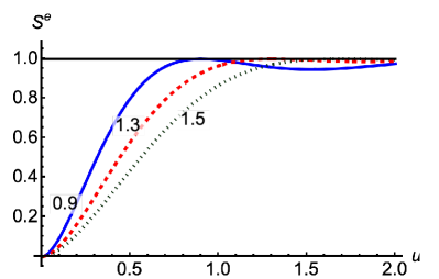
Figure 2: $S^{e}$ as a function of the dimensionless variable $u$ for the three different values of $v$. The values of $v$ are 0.9 (solid), 1.1 (dashed) and 1.3 (dotted) . These values correspond to total cross sections of 22 mb, 40 mb and 56 mb.

The case with $U=\pm V$ yields $P_{G}^{e}=P_{X}^{e}=1/2$, and a maximum of entropy. This corresponds to the total absorption limit in which elastic and inelastic cross sections are equal. This means that the black disk limit corresponds to maximum scattering entropy.

Presenting a brief discussion of the total absorption limit is worthwhile. The partial wave decomposition of the scattering amplitude $f(\theta)$ for a spinless particle is:

$$f(\theta)={-i\over 2k}\sum_{l}(2l+1)(\eta_{l}-1)P_{l}(\cos\theta).$$ (37)

The strong absorption model is defined by $\eta_{l}=0$ for $l\leq L$ and $\eta_{l}=1$ for $l>L$, with $L\approxeq kR$. The sum is then given by $f(\theta)\approx{i\over k}L(L+1){J_{1}(L\theta)\over L\theta}$, a form familiar form Frauenhoffer diffraction. In nuclear physics this is known as the Blair model Blair (1954); Ericson (1966). See  Abul-Magd and Simbel (1970). Data were reproduced using a distribution without a sharp edge, for example $\eta_{l}=1/(1+\exp{(L-l)/b})$ with $b>1/2$. This is a grey disc model.

To see if the total absorption or grey disc model is is a result of the present calculation, I provide a specific example, based on parameters typical of proton-proton scattering Use a Gaussian density function $\rho(r)=\exp((-r^{2})/R^{2})$, where $R$ is the radius parameter, taken here as $\sqrt{2}$ fm obtained by convoluting Gaussian densities, of radius parameter 1 fm) of two protons. Then let $V(r)=V_{0}\rho(r)$ and $U(r)=U_{0}\rho(r)$. Treating $u$ and $v$ as constants corresponds to treating the interactions as coming from vector exchanges-the typical treatment of high-energy hadron-hadron scattering. The value of scattering entropy is then independent of energy for sufficiently high energies. In line with the high-energy behavior, I define $v\equiv 2\lambda_{V}k$ and $u\equiv 2\lambda_{U}k$ so that evaluation of Eq. (29) yields the results $\delta_{V,U}(b)=\lambda_{V,U}\sqrt{\pi}R\exp(-b^{2}/R^{2})$. Then using Eq. (30), a value of $\lambda_{V}$ of about 100 MeV gives a total cross section of about 40 mb, the typical value of the high-energy, proton-proton cross section.

The results, independent of the signs of $U_{0}$ and $V_{0}$, are shown in Fig. 2 in terms of $u\equiv\lambda_{U}\sqrt{\pi}R$ and $v\equiv\lambda_{V}\sqrt{\pi}R$. Maximum entanglement is reached, as expected, for cases with $u=v$. Observe that, except for very small values of $u$ (small inelastic scattering) the entanglement entropy is always substantial.

It is useful to learn if the results of the present calculation correspond to the total absorption or gray disc model. To do this, refer to Eq. (27) and define $\eta(b)\equiv e^{-i\delta_{V}(b)}\cos\delta_{U}(b)$. This quantity is shown in Fig. 3 for the case $u=v=1.3$. The present calculation is seen to correspond to the grey disc model, not far from the total absorption model.

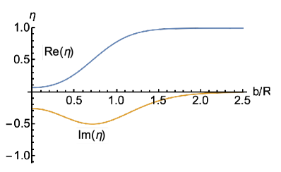
Figure 3: Real and imaginary parts of $\eta(b)$.

IV Extension to more than one excited state and a general result

Can the models of the previous two models be extended to include more than one excited state? What then can one say about entanglement? If there is more than one excited state, a single measurement of the projectile energy cannot be used to determine the specific excited state of the target. The entanglement properties are then unknown.

However, a single measurement of the projectile energy can determine whether or not the target is excited. Therefore it seems sensible to consider the previous terms $P_{X}$ and $P^{e}_{X}$ to represent the probability that the target has been excited to any excited. In that case, the expressions for the scattering entropy of Eq. (17) and Eq. (36) can be thought of as general measures of entanglement for any projectile-target system that involves inelastic excitation.

V high energy proton-proton scattering

Data for total cross sections and total elastic cross sections are available from the Particle Data Group Workman and Others (2022). Then, the high-energy analysis presented above can be used with the identifications: $P_{G}=\sigma_{\rm el}/\sigma_{\rm tot},\,P_{X}=1-P_{G}$ along with Eq. (36). The results are shown in Fig. 4.

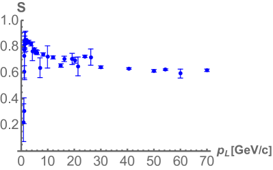
Figure 4: $S^{e}$ as a function of the fixed-target laboratory momentum $p_{L}$..

At low energies there is no inelastic scattering, so the scattering entropy must vanish. This result is similar to the results shown in Fig. 1 for small values of $k$. and to Fig. 2 for small values of $u$. As energies rise above inelastic scattering thresholds the entanglement increases. At still higher energies the ratio of elastic to total cross sections is approximately flat. The entanglement entropy is substantial at laboratory momenta greater than about 2 GeV/c (kinetic energy about 1.3 GeV). At higher energies than are shown $S$ is approximately flat with energy because the ratio $\sigma_{|rmel}/\sigma_{\rm tot}$ is approximately independent of energy.

The large value of entanglement entropy indicates that the total absorption or gray disc model are reasonable first approximations to understanding the data. The net result is that computing the entanglement energy provides insight regarding the underlying dynamics of proton-proton scattering, in particular and more generally of projectile-target scattering.

This work was supported by the U. S. Department of Energy Office of Science, Office of Nuclear Physics under Award Number DE-FG02-97ER-41014.

References

- Ehlers (2022) Peter J. Ehlers, “Entanglement between Valence and Sea Quarks in Hadrons of 1+1 Dimensional QCD,” (2022), arXiv:2209.09867 [hep-ph] .
- Kharzeev and Levin (2017) Dmitri E. Kharzeev and Eugene M. Levin, “Deep inelastic scattering as a probe of entanglement,” Phys. Rev. D 95, 114008 (2017), arXiv:1702.03489 [hep-ph] .
- Feal et al. (2019) X. Feal, C. Pajares, and R. A. Vazquez, “Thermal behavior and entanglement in pb-pb and collisions,” Phys. Rev. C 99, 015205 (2019).
- Gotsman and Levin (2020) E. Gotsman and E. Levin, “High energy qcd: Multiplicity distribution and entanglement entropy,” Phys. Rev. D 102, 074008 (2020).
- Hentschinski et al. (2022) Martin Hentschinski, Krzysztof Kutak, and Robert Straka, “Maximally entangled proton and charged hadron multiplicity in Deep Inelastic Scattering,” Eur. Phys. J. C 82, 1147 (2022), arXiv:2207.09430 [hep-ph] .
- Wang and Chen (2015) Rong Wang and Xurong Chen, “Valence quark distributions of the proton from maximum entropy approach,” Phys. Rev. D 91, 054026 (2015).
- Beane and Ehlers (2019) Silas R. Beane and Peter Ehlers, “Chiral symmetry breaking, entanglement, and the nucleon spin decomposition,” Mod. Phys. Lett. A 35, 2050048 (2019), arXiv:1905.03295 [hep-ph] .
- Beane et al. (2019) Silas R. Beane, David B. Kaplan, Natalie Klco, and Martin J. Savage, “Entanglement Suppression and Emergent Symmetries of Strong Interactions,” Phys. Rev. Lett. 122, 102001 (2019), arXiv:1812.03138 [nucl-th] .
- Liu et al. (2023) Qiaofeng Liu, Ian Low, and Thomas Mehen, “Minimal entanglement and emergent symmetries in low-energy QCD,” Phys. Rev. C 107, 025204 (2023), arXiv:2210.12085 [quant-ph] .
- Miller (2023) Gerald A. Miller, “Entanglement Maximization in Low-Energy Neutron-Proton Scattering,” (2023), arXiv:2306.03239 [nucl-th] .
- Bai (2023) Dong Bai, “Spin entanglement in neutron-proton scattering,” (2023), arXiv:2306.04918 [nucl-th] .
- Bai and Ren (2022) Dong Bai and Zhongzhou Ren, “Entanglement generation in few-nucleon scattering,” Phys. Rev. C 106, 064005 (2022), arXiv:2212.11092 [nucl-th] .
- Johnson and Gorton (2023) Calvin W. Johnson and Oliver C. Gorton, “Proton-neutron entanglement in the nuclear shell model,” J. Phys. G 50, 045110 (2023), arXiv:2210.14338 [nucl-th] .
- Kruppa et al. (2021) A. T. Kruppa, J. Kovács, P. Salamon, and Ö. Legeza, “Entanglement and correlation in two-nucleon systems,” J. Phys. G 48, 025107 (2021), arXiv:2006.07448 [nucl-th] .
- Kruppa et al. (2022) A. T. Kruppa, J. Kovács, P. Salamon, Ö. Legeza, and G. Zaránd, “Entanglement and seniority,” Phys. Rev. C 106, 024303 (2022), arXiv:2112.15513 [nucl-th] .
- Robin et al. (2021) Caroline Robin, Martin J. Savage, and Nathalie Pillet, “Entanglement Rearrangement in Self-Consistent Nuclear Structure Calculations,” Phys. Rev. C 103, 034325 (2021), arXiv:2007.09157 [nucl-th] .
- Pazy (2023) Ehoud Pazy, “Entanglement entropy between short range correlations and the Fermi sea in nuclear structure,” Phys. Rev. C 107, 054308 (2023), arXiv:2206.10702 [nucl-th] .
- Tichai et al. (2022) A. Tichai, S. Knecht, A. T. Kruppa, Ö. Legeza, C. P. Moca, A. Schwenk, M. A. Werner, and G. Zarand, “Combining the in-medium similarity renormalization group with the density matrix renormalization group: Shell structure and information entropy,” (2022), arXiv:2207.01438 [nucl-th] .
- Gu et al. (2023) Chenyi Gu, Z. H. Sun, G. Hagen, and T. Papenbrock, “Entanglement entropy of nuclear systems,” (2023), arXiv:2303.04799 [nucl-th] .
- Bulgac (2022) Aurel Bulgac, “Entanglement entropy, single-particle occupation probabilities, and short-range correlations,” (2022), arXiv:2203.12079 [nucl-th] .
- Bulgac et al. (2023) Aurel Bulgac, Matthew Kafker, and Ibrahim Abdurrahman, “Measures of complexity and entanglement in many-fermion systems,” Phys. Rev. C 107, 044318 (2023), arXiv:2203.04843 [nucl-th] .
- Cervera-Lierta et al. (2017) Alba Cervera-Lierta, José I. Latorre, Juan Rojo, and Luca Rottoli, “Maximal Entanglement in High Energy Physics,” SciPost Phys. 3, 036 (2017), arXiv:1703.02989 [hep-th] .
- Kovchegov and Levin (2013) Yuri V. Kovchegov and Eugene Levin, Quantum Chromodynamics at High Energy, Vol. 33 (Oxford University Press, 2013).
- Frauenfelder and Henley (1991) H. Frauenfelder and E. M. Henley, Subatomic Physics Second Edition (Prentice-Hall, 1991).
- Gottfried (2018) Kurt Gottfried, Quantum:Mechanics Value I:Fundamentals (CRC Press, Boca Raton, 2018).
- Kamal and Kreuzer (1970) A. N. Kamal and H. J. Kreuzer, “Soluble two-channel problems in potential scattering,” Phys. Rev. D 2, 2033–2039 (1970).
- Glauber (1959) R. J. Glauber, “Lectures in theoretical physics,” (Interscience Publishers, New York, 1959) Chap. 3, pp. 315–415.
- Blair (1954) J. S. Blair, “Theory of Elastic Scattering of Alpha Particles by Heavy Nuclei,” Phys. Rev. 95, 1218–1222 (1954).
- Ericson (1966) T. E. O. Ericson, “Preludes in theoretical physics,” (North Holland, Amsterdam, 1966) pp. 321–329.
- Abul-Magd and Simbel (1970) A. Y. Abul-Magd and M. H. Simbel, “THE ACCURACY OF THE INOPIN-ERICSON THEORY OF NUCLEAR DIFFRACTION SCATTERING,” Nucl. Phys. A 148, 449–456 (1970).
- Workman and Others (2022) R. L. Workman and Others (Particle Data Group), “Review of Particle Physics,” PTEP 2022, 083C01 (2022).