Bulk-preventing actions for SU(N) gauge theories
Abstract
Lattice gauge field theories may suffer from unphysical ”bulk” phase transitions at strong lattice gauge coupling. We introduce a one-parameter family of lattice gauge actions which, when used in combination with an HMC update algorithm, prevents the appearance of the bulk phase transition. We briefly discuss the (presumed) mechanism behind the prevention of the bulk transition and present test results for different gauge groups.
I Introduction
In asymptotically free gauge theories on the lattice the continuum limit is obtained when the bare lattice gauge coupling vanishes. In practice lattice simulations are always done at finite lattice spacing, and as long as the coupling constant is sufficiently small we can analytically extrapolate the results to the continuum limit. The range of lattice spacings (or coupling constants) is often limited by the emergence of an unphysical “bulk phase” at strong lattice gauge coupling, which prevents the analytical connection to the continuum phase from this region. The value of the lattice coupling where the transition to the bulk phase happens depends on the lattice gauge group, the choice of the gauge action and the matter content.
The problem of the bulk phase transition becomes acute in gauge theories with large number of colors and in models with large number of fermion degrees of freedom. In pure gauge theories with the standard Wilson plaquette action the bulk transition is a rapid cross-over if but becomes an increasingly strong first order transition for [1]. Adding fermionic degrees of freedom slows down the evolution of the coupling constant (i.e. the magnitude of the -function is smaller) and also increase the effective lattice gauge coupling [2]. Depending on the physical case of interest, these effects require one to use strong bare coupling. This happens especially in infrared (near-)conformal models, where the coupling runs very slowly, for example in with large numbers of fundamental fermions [3, 4, 5, 6, 7], with adjoint fermions [8, 9, 10], with large Nf [11, 12, 13], and with fermions in the antisymmetric representation [14].
In this work we present a local lattice gauge action, defined on elementary plaquettes, which efficiently removes the transition to the bulk phase. Our approach is related to the ”dislocation prevention” method by DeGrand et al. [15]. For and gauge groups also the topological gauge actions that restict the plaquette magnitude [16, 17, 18] are to some extent related. The latter stops being the case for gauge groups with , as the plaquette eigenvalues are then no longer determined by the trace of the plaquette. We note that our approach removes merely the bulk phase but does not restrict in any way gauge-topology fluctuations.
Following Wilson’s prescription, the lattice discretization of a gauge theory is obtained by promoting the Lie algebra valued continuum gauge field,
| (1) |
with being a basis of , to Lie group valued link variables,
| (2) |
which can be interpreted as the gauge-parallel transporters along the link between a site and a neighboring site . The leading on the right-hand side of (2) indicate that path-ordering should be applied when evaluating the exponential of the line-integral. The relation between the coordinate in (1) and the coordinate in (2) is given by , where is the lattice spacing, and refers to the unit-vector in -direction. Parallel transporters over longer distances are then expressed as products of consecutive link variables and a lattice gauge action can be defined in terms of link variables by requiring that in the limit the lattice gauge action converges to the continuum gauge action,
| (3) |
Wilson proposed the gauge action [19]
| (4) |
which, as is well known, satisfies the above condition and is here written in terms of the inverse bare gauge coupling and the plaquette variables
| (5) |
The gauge action (4) and improved versions of it [20] are the most commonly used in Monte Carlo studies of lattice gauge theories. They are, however, not unique and might not be the best choice for the study of lattice gauge theories at strong coupling, as they allow the gauge system to enter the bulk phase. Despite its name, the bulk phase is not necessarily a proper phase, but simply a region in parameter space of the lattice theory where lattice artifacts dominate in ensemble averages. As a consequence the relation between lattice and continuum results becomes very complicated or can even be lost completely if bulk and continuum phase are separated by a first order transition.
II Avoiding the lattice bulk phase
In this section we propose a characterization of ”bulk configurations” in lattice gauge systems, which allows for the definition of a family of lattice gauge actions, that separate such bulk configurations from regular ones by an infinite potential barrier, while still yielding the same naive continuum limit as Wilson’s plaquette gauge action. In combination with a hybrid Monte Carlo (HMC) update algorithm, the new gauge actions prevent the gauge system from entering a bulk phase.
II.1 Motivation in
In the case, the Wilson gauge action in (4) reduces to
| (6) |
and the Abelian link variables can be written as
| (7) |
Let us now define,
| (8) |
and note that while in (8) can vary in the interval , the gauge action (6) depends only on
| (9) |
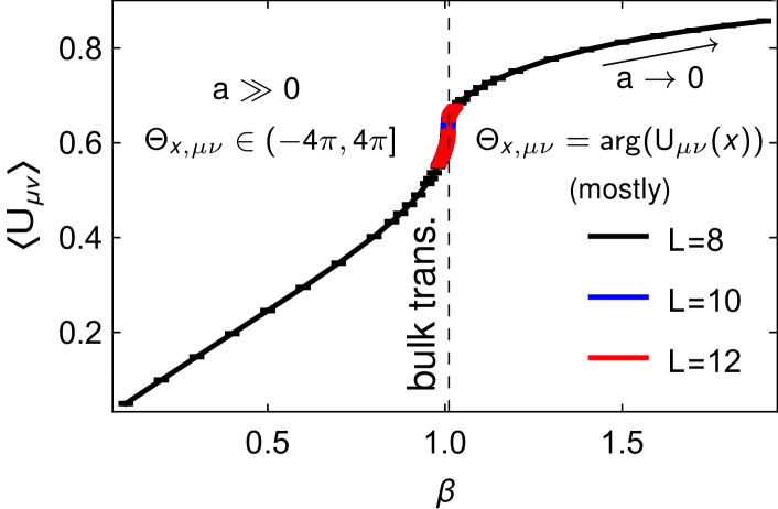
As illustrated in Fig. 1, the gauge action (6) produces a bulk-transition at . For , the system is in the bulk phase, where the lattice spacing, , can be considered large and from (8) explores the full -interval. For , the system is in the continuum phase, where the lattice spacing tends to zero if . In this phase, can still be outside the -interval, but the fraction of such plaquettes quickly drops as and most of the time, one has that .
-
(a)
link wraps around -interval:
-
(b)
grows continuously:
The fact that plaquettes with also appear in the continuum phase indicates that the value of by itself cannot be used to distinguish bulk from continuum configurations. However, as illustrated in Fig. 2, for smoothly varying link variables, , one can identify two qualitatively different ways in which plaquettes with can be produced from a configuration in which initially is satisfied for all plaquettes:
-
(a)
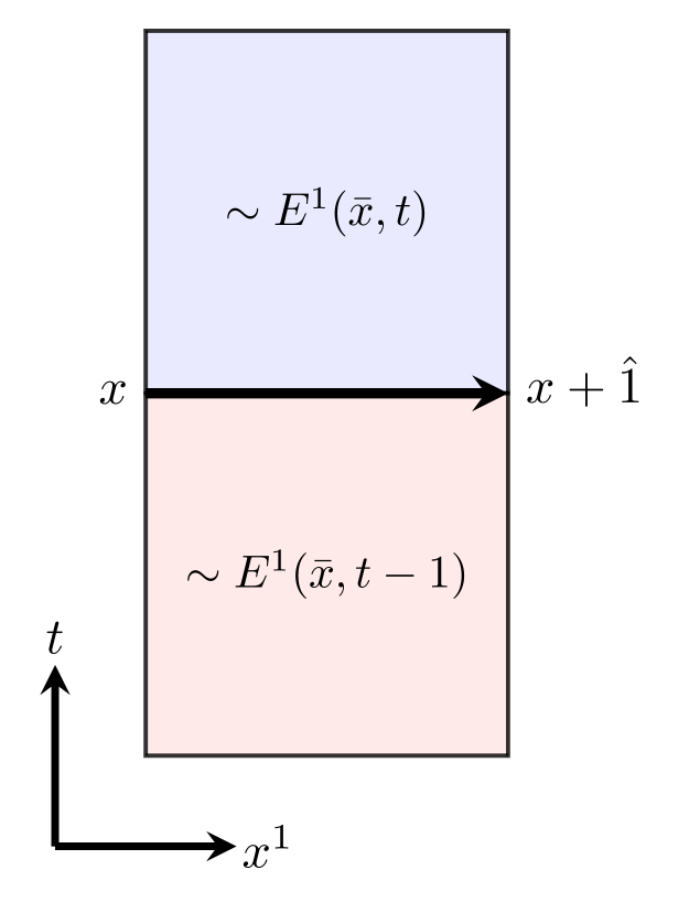
the phase of one of the links of a given plaquette can move across the boundary of the -interval and wrap around, which adds roughly to the plaquette’s phase angle . As indicated in part (a) of Fig. 2, this kind of plaquette wrapping can happen also if is close to . We note that the wrapping link will produce a shift of roughly in the phase angle of all plaquettes that contain this link and not just in the phase angle of the plaquette under consideration;
-
(b)
none of the links of a given plaquette wraps around the -interval. Instead, as indicated in part (b) of Fig. 2, the plaquette’s phase angle has grown close to the -interval boundary and finally crosses it continuously as one of the link variables undergoes a change that causes to grow further. Unlike in case (a), this continuous plaquette wrapping can take place for single plaquettes. This can produce metastabilities as wrapped and unwrapped plaquettes pull in opposite directions on shared links when the action is minimized. In order to approach the continuum limit, the wrapping needs to be undone.
As case (b) can occur only if individual plaquette angles are allowed to grow close to , this case is likely to occur only in the bulk phase, where is so small that the plaquette action (6) cannot grow sufficiently large as to oppose the entropy-driven randomization of the plaquette variables in the system. We will therefore introduce in Sec. II.3 a family of actions that will prevent plaquette wrappings of type (b). As it turns out, this is sufficient to get rid of the bulk transition. First, however, we discuss in Sec. II.2 how the concept of continuous type (b) plaquette wrappings can be generalized from to plaquettes. The relation between plaquette wrappings and the production of Dirac monopoles is discussed in Appendix A.1.
II.2 Situation in
Compact Lie groups like carry a Riemannian metric which is invariant under left and right translation. As a consequence, the well known bi-invariant Haar measure for group integration exists, which is given by the volume form of the invariant metric, normalized so that that the group volume is . The fact that has a Riemannian metric also means that we can at each point define a tangent space and the so called exponential map that maps vectors from the tangent space at point to points in . The graph of the function , then describes a geodesic segment in that start in the point in the direction specified by and has geodesic length .
The exponential map is bijective only in a neighborhood around the origin of . The boundary of the region over which the exponential map is bijective is called the cut locus of in and its image is, correspondingly, the cut locus of in .
At the point the tangent space to corresponds to the usual Lie algebra and the exponential map applied to some can be identified with the usual matrix exponential,
| (10) |
with being a hermitian basis of .
The domain over which is bijective is given by the set of hermitian matrices whose eigenvalues satisfy [21]:
| (11) |
The image , i.e. the cut locus of in , is therefore given by the set of matrices for which at least one eigenvalue , is equal to .
To illustrate this, we pick a and write it as
| (12) |
with and being a diagonal matrix containing the eigenvalues of . The image of under the exponential map is then,
| (13) |
with being the diagonal matrix of eigenvalues of , given by , . As long as , the exponential map is a bijection as the inverse map can be defined using,
| (14) |
with being the principal value complex logarithm. But, if for any , then (14) breaks down.
We can now generalize the criterion we found in the previous section for the production of bulk configurations in lattice gauge theory to the case. In the case we argued, that if the phase (8) of any plaquette variable in the system crosses continuously the -interval boundary (plaquette wrappping of type (b)), then a bulk configuration is produced. Such a continuous crossing of the -interval boundary by the plaquette phase implies of course that the corresponding plaquette variable passes through the value , which is the cut locus for the exponential map from the Lie algebra to the group manifold . If a plaquette variable approaches and smoothly crosses the cut locus value the resulting lattice gauge field described by the link variables can no longer be properly mapped on a corresponding Lie algebra valued gauge field that is relevant for continuum physics. The same applies in the case of lattice gauge theory if a plaquette variable approaches and smoothly cross the cut locus. The resulting configuration cannot be mapped on a corresponding Lie algebra valued gauge configuration that is relevant for continuum physics, which qualifies it as a bulk configuration.
In order to prevent a gauge system form entering a bulk phase at strong coupling, the plaquette variables must not continuously cross the cut locus. As discussed below (11), this means that the eigenvalues of the plaquette variables must not continuously cross the value .
The question of how such a restriction affects the creation of magnetic monopoles in gauge theory is addressed in Appendix A.2.
II.3 Bulk-preventing action
To prevent plaquettes from having eigenvalues close to , we introduce the following family of gauge actions:
| (15) |
with and
| (16) |
The form of the actions (15) was inspired by the dislocation-prevention action introduced in [15]. The naive continuum limit of (15) is the same as for the Wilson gauge action . This can be seen by writing , with and expanding in a power series in . For the local plaquette action contributing to from (4) one then finds:
| (17) |
and, correspondingly, for the local plaquette action contributing to from (15):
| (18) |
In the limit , one has , , and we see that the two local actions have the same leading term , namely:
| (19) |
The actions (15) introduce an infinite potential barrier between bulk and continuum configurations. This is sufficient to ensure that, if we start a simulation from a cold configuration (all link variables equal to the identity) and use a hybrid Monte Carlo (HMC) algorithm to update the gauge system, no bulk-configurations will be produced.
One could infer that our bulk-preventing setup results in a non-ergodic update algorithm. However, one should keep in mind that the part of the configuration space that is not sampled is irrelevant for the continuum limit of the theory. The algorithm prevents ensemble averages of the lattice system from being contaminated (or even dominated) by bulk-configurations, which should allow one to extract continuum physics also at stronger coupling. The same effect could be achieved by defining a modified measure, which gives zero weight to bulk configurations. However, this would be difficult to implement as the latter are hard to identify once they are created. The use of an action (15) in combination with an HMC algorithm is a proxy to achieve the same effect but in a simpler and more economic way. An expression for the gauge force, required for the HMC, is presented in Appendix B.
Let us note that for and , the actions in (15) alone would have a similar effect as the topological actions discussed in [22, 16, 17, 18]: the larger the inverse bare coupling , the stronger the plaquette values are repelled from resp. . For with the effect of (15) is, however, different from the one of the topological action discussed in [18], as for the trace of the plaquette does no-longer completely determine the plaquette eigenvalues. An action which can have a similar effect as our actions (15) has been given in [23]. We also note that based on the observation that the bulk transition of the Wilson gauge action (4) is sensitive to the addition of an adjoint plaquette term [24], it has in [25] been demonstrated that for the bulk phase can be avoided by adding an appropriately scaled negative adjoint plaquette term to the standard Wilson gauge action [26, 25].
III Results
To test whether the bulk-preventing actions (15) deserve their name and whether they are able to reproduce the same weak coupling results as the Wilson gauge action, we carried out simulations with pure gauge , pure gauge , and with Wilson fermion flavours. With the Wilson gauge action, all three of these theories enter a bulk phase for sufficiently small values of the inverse gauge coupling . For pure gauge , the transition is a smooth cross-over, while for pure gauge and for the fermionic theory with sufficiently large fermion hopping parameter the transition is of first order. In the following we will discuss the three cases separately. We use the version of the action (15) with . The choice of should not affect physical results, but it turns out that a too small value of will require also a smaller step size in the HMC trajectories to achieve similar acceptance rates, which can become computationally more expensive than using .
According to the expansions (17) and (18), the Wilson gauge (WG) action (4) and bulk-preventing (BP) action (15) agree only to order . Thus, the inverse bare couplings and will not be equal in the weak coupling limit. However, it turns out that locally the two couplings can be related quite accurately by a constant shift, , which we will use to directly compare bare lattice results obtained with the two different actions. Of course, there is in general no need for bare lattice results, obtained with different actions, to agree. However, it seems that in the present case, the systems controlled by the WG and the BP action behave in the weak coupling regime sufficiently equally, so that a direct comparison of bare lattice results is reasonable.
III.1 pure gauge
pure gauge theory with the WG action (4) is known to have a smooth cross-over between the bulk phase and the continuum-like phase. Thus, for this theory the BP action (15) is not expected to provide any significant advantage over the WG action and both actions should give rise to the same results not just at weak, but also all the way down to strong coupling.
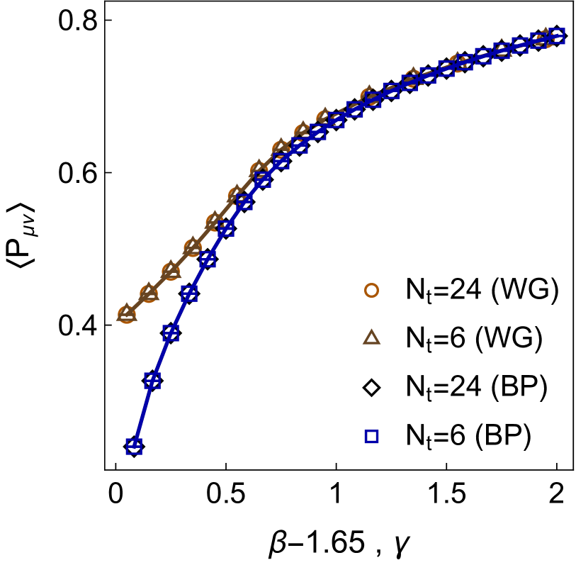
In Fig. 3 we compare results obtained with the WG and the BP action. The WG data is plotted as function of with and the BP data is plotted as function of . The shift has been determined by requiring that the ”spatial deconfinement” transition, at which the spatial Polyakov loop develops a non-zero expectation value (indicating that the physical spatial volume becomes too small to fit a meson), occurs for the two actions at the same value of resp. .
The top-left panel in Fig. 3 shows the average of the traced plaquette and we note that when plotted against resp. , the plaquette values for the two different actions agree remarkable well at sufficiently weak coupling. Only below , where the WG action enters the bulk-phase, the plaquette value for the WG action starts to deviate from the BP one as function of .
The strong coupling limit is for both actions obtained by sending their respective inverse coupling to zero, i.e. and . With the WG action the strong coupling phase extends over the interval , while with the BP action, the strong coupling phase extends over the significantly smaller interval . In the strong coupling phase, the system should therefore with the WG action change more slowly as function of than with the BP action as function of .
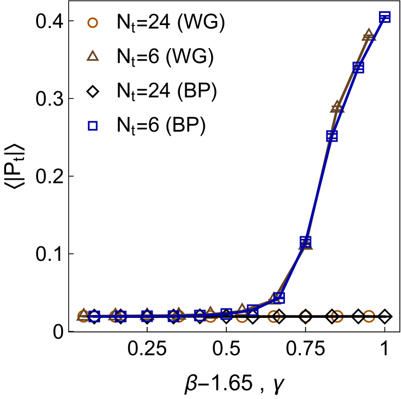
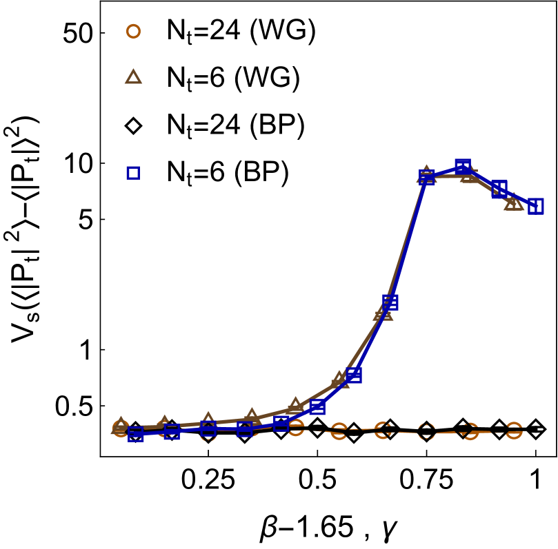
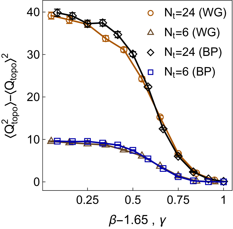
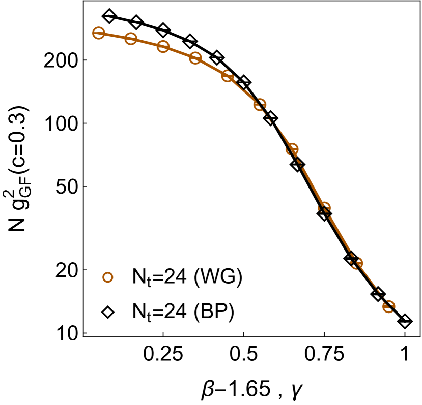
This is indeed what can be observed in the remaining panels of Fig. 3: the results obtained with the two actions for temporal Polyakov loop (top-center), Polyakov loop variance (top-right), and topological susceptibility (bottom-left) are consistent and match for very nicely as functions of resp. , while for , the WG results change more slowly as function of than the corresponding BP results do as function of .
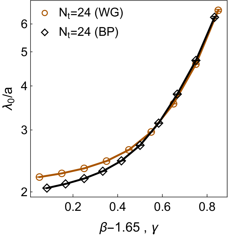
The last two panels on the second row of Fig. 3 show gradient flow quantities: the bottom-center panel shows the gradient flow coupling, at , with being the flow scale corresponding to flow time ; and the bottom-right panel shows , which is the flow scale (in lattice units) at which [28] with being the clover action density of the flowed gauge field at flow time . Both gradient flow quantities have been corrected for leading finite volume and lattice spacing effects [7] by replacing in the computation of the continuum finite volume correction given in [29] the continuum momenta by lattice momenta and adapting the formula to the case . A refined correction formula that takes into account the details of the utilized lattice actions for sampling and flowing of the gauge fields, as well as for measuring , is presented in [30]. Also for the gradient flow quantities the data obtained with the two actions agrees as function of if , whereas for , the WG data changes more slowly as function of than the BP data does as function of .
As mentioned at the beginning of this section, the shift has been determined by requiring that the spatial deconfinement happens at the same value of and . Because of our small spatial volumes of linear size , this happens already at .
III.2 pure gauge
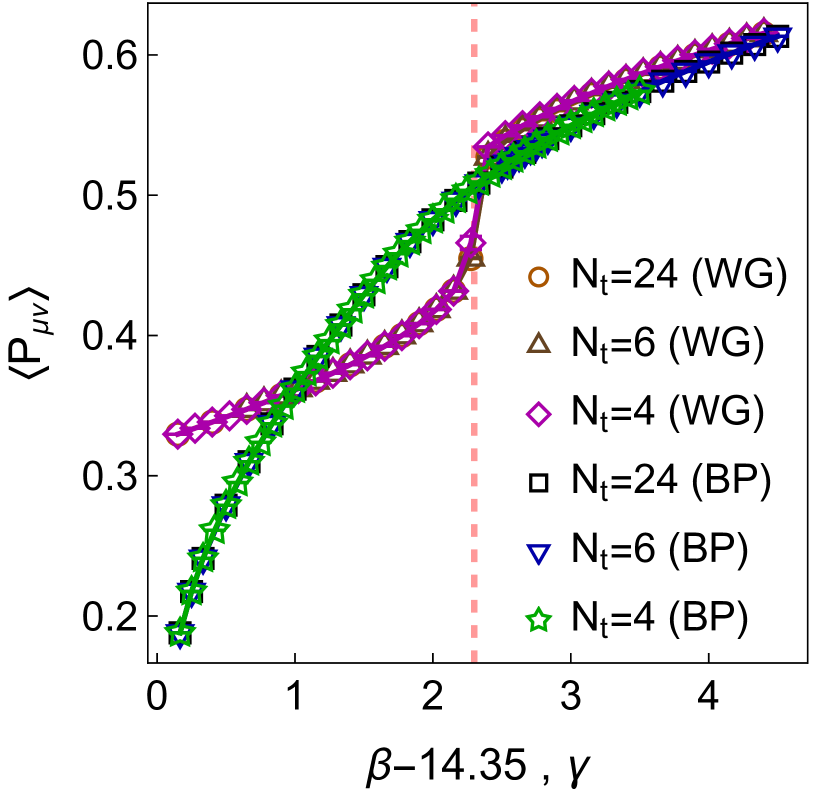
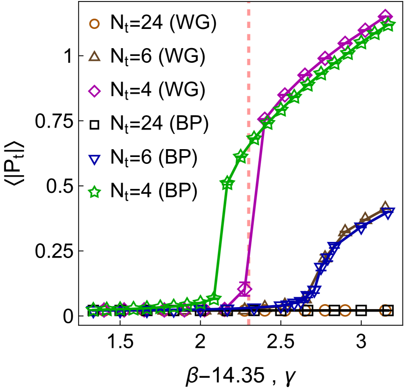
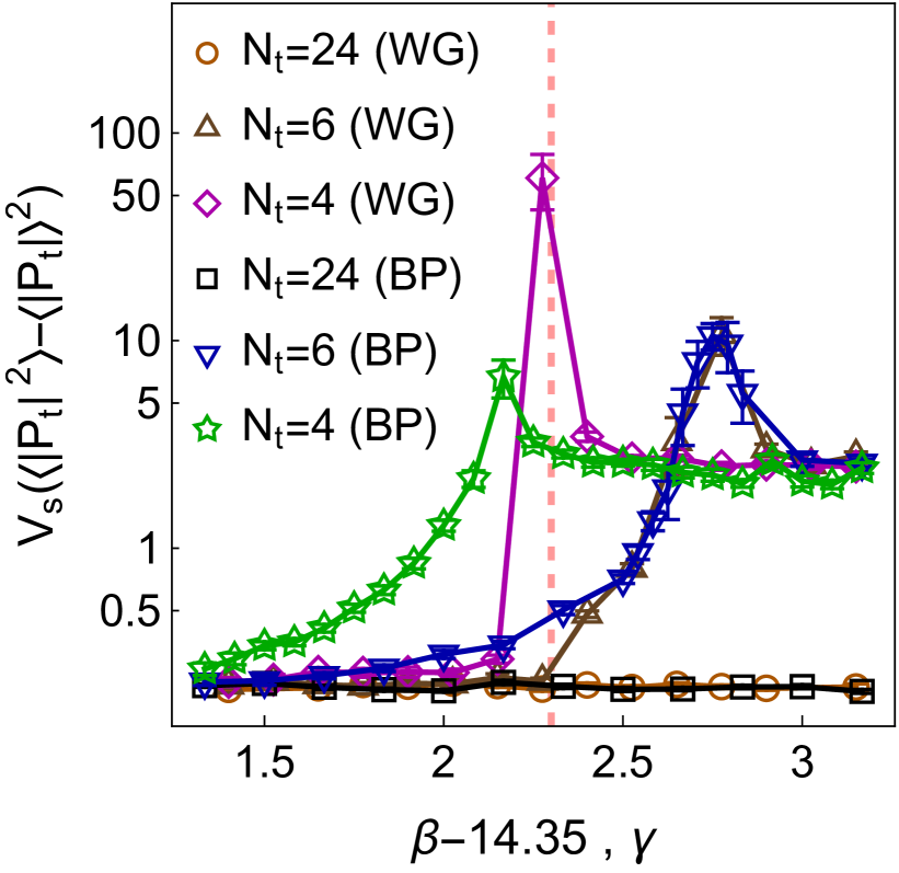
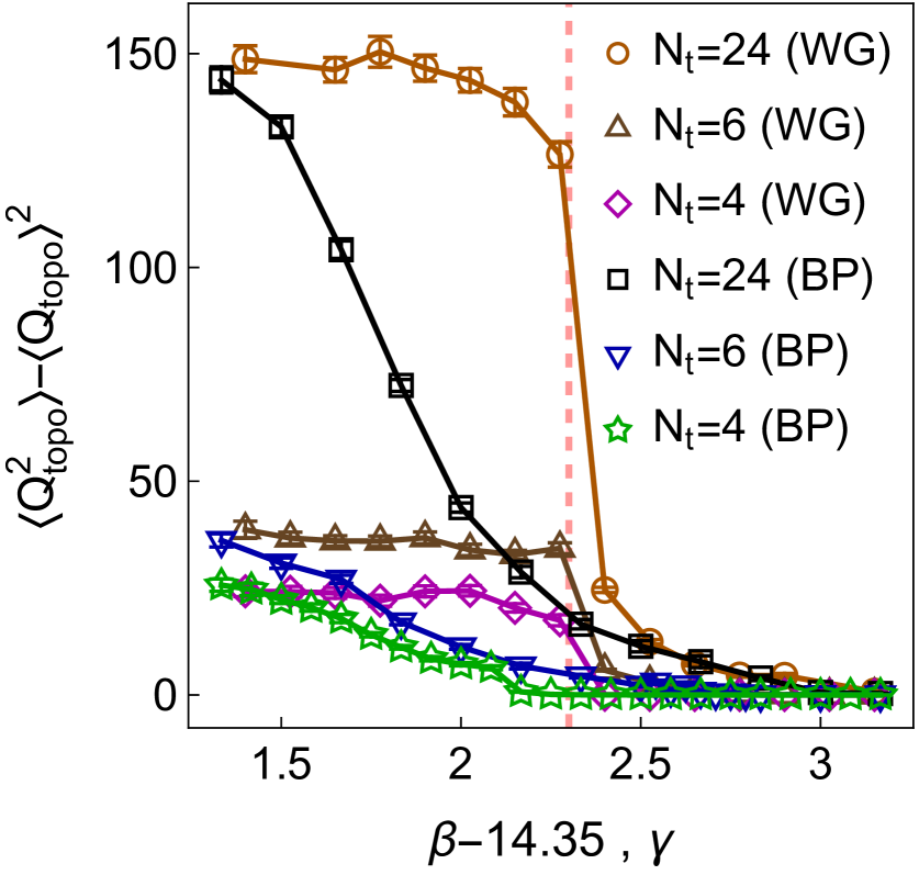
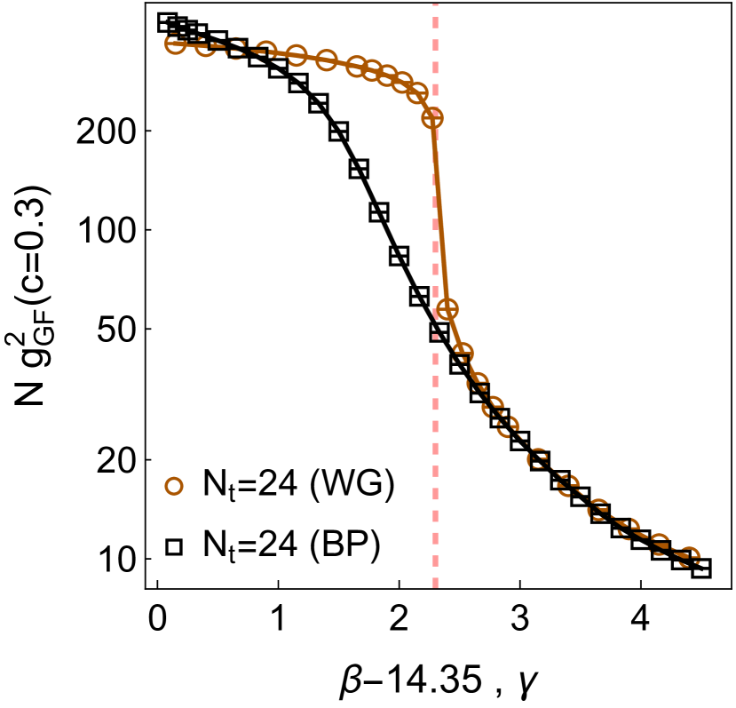
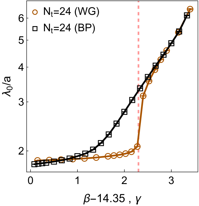
Fig. 4 provides the same information as Fig. 3 but for instead of . The shift in required to match at weak coupling has been set to , which, as in the -case, is determined by matching the values of and at which spatial deconfinement occurs.
For the bulk transition of the WG action is of 1st order [1], which is clearly visible from the sharp discontinuity in the WG data for the average plaquette at , shown in the top-left panel of Fig. 4. In contrast, with the BP action the plaquette is completely continuous as a function of the inverse gauge coupling . In the continuum phase, i.e. for , the average plaquette values obtained with the two different actions converge only slowly with increasing inverse coupling, while the average temporal Polyakov loop (top-center), temporal Polyakov loop variance (top-right) and topological susceptibility (bottom-left), as well as the gradient flow quantities, (bottom-center) and (bottom-right), agree for the two actions almost immediately when .
The finite temperature transition for occurs at around . This is above the value at which the WG action undergoes the bulk transition, and the properties of the finite temperature transition should therefore be described equally well with the WG and with the BP action. The temporal Polyakov loop (top-center) looks indeed the same for the two actions at , and also the temporal Polyakov loop variance (top-right) agrees very well for at ; at (red vertical dashed line) one can, however, notice a small jump in the Polyakov loop variance for the WG action, while the Polyakov loop variance obtained with the BP action behaves completely regular across this point.
A similar behavior can be observed in the data for the topological susceptibility (bottom-left), where the results obtained with the WG and BP action agree for , but as decreases below the bulk transition point, , the topological susceptibility obtained with the WG action jumps and approaches almost immediately its strong-coupling plateau value, while with the BP action, the topological susceptibility approaches its strong coupling value much more smoothly.
With , the WG action is no longer able to properly resolve the finite temperature transition. The data obtained with the BP action suggests that the finite temperature transition should for occur at . With the WG action, the system is in the bulk-phase at this value of the bare gauge coupling [1]. It appears that the finite temperature transition cannot take place inside the bulk phase and occurs therefore on top of the bulk transition. Also the topological susceptibility obtained with the WG action for appears to be unable to decrease as long as the system is in the bulk phase. As in the case of , the topological susceptibility obtained with the WG action appears also for to be stuck at the strong coupling plateau value for and to decrease abruptly at when the inverse coupling is increased beyond this point. In contrast, with the BP action the asymptotic strong coupling value of the topological susceptibilities is also for approached smoothly.
The measurements of the gradient flow coupling at are shown in the bottom-center panel of Fig.4. From this we conclude that the WG action is not capable of reaching gradient flow couplings larger than before hitting the bulk transition. In the bottom-right panel we show the flow scale at which [28]. For the WG action there is a discontinuity in at the bulk transition point, indicating that there is a largest reachable lattice spacing. For the BP action these problems disappear and the gradient flow quantities behave smoothly. As in the case, both gradient flow quantities have been corrected for finite volume and finite lattice spacing effects.
III.3 with Wilson fermions
For a lattice gauge theory with the Wilson gauge action, the transition between continuum- and bulk-phase is normally a cross-over. However, if the theory is coupled to fermions, the transition can turn 1st order.
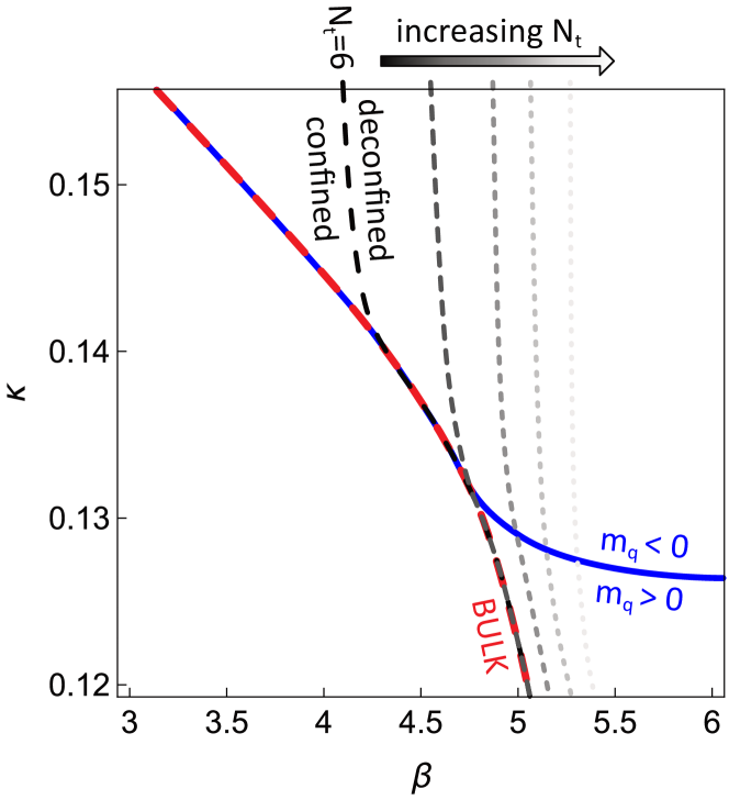

As a concrete example for a system where this is the case, we consider lattice gauge theory with the WG action and with mass-degenerate, dynamical Wilson-clover fermion flavors, that couple to the gauge field via 2-step stout smeared links. Fig. 5 shows a schematic -phase diagram for this system. The dashed red line marks the location of the bulk transition, the blue line indicates where the PCAC quark mass, , crosses zero, and the dashed black line marks the location of the thermal resp. ”confinement/deconfinement” transition if the temporal lattice size is set to . The label ”confinement/deconfinement” is put in quotation marks, because we use the temporal Polyakov loop as approximate order parameter for deconfinement, despite the presence of dynamical fermions [31, 32]. In QCD deconfinement is observed to be accompanied by a chrial transition that occurs at the same temperature; for light fermions, this chiral transition dominates, whereas in the heavy fermion limit, the ”confinement/deconfinement” transition of pure gauge theory is approached.
The curves in Fig. 5 are based on parameter scans performed with simulations on lattices of spatial size with . For the and the bulk transition lines, the temporal lattice extent was set to (approximating zero-temperature), while for the ”confinement/deconfinement” transition, the indicated was used. The additional dashed lines in different shades of gray are not based on actual simulations; they merely illustrate how the ”confinement/deconfinement” transition line is expected to change if is increased (assuming that also is increased accordingly).
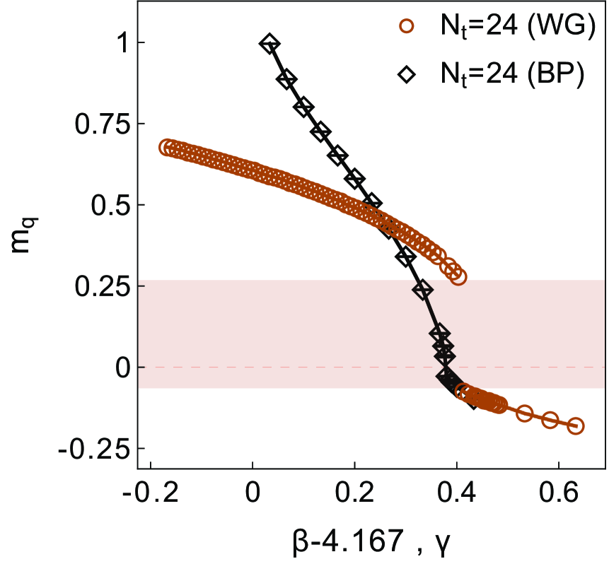
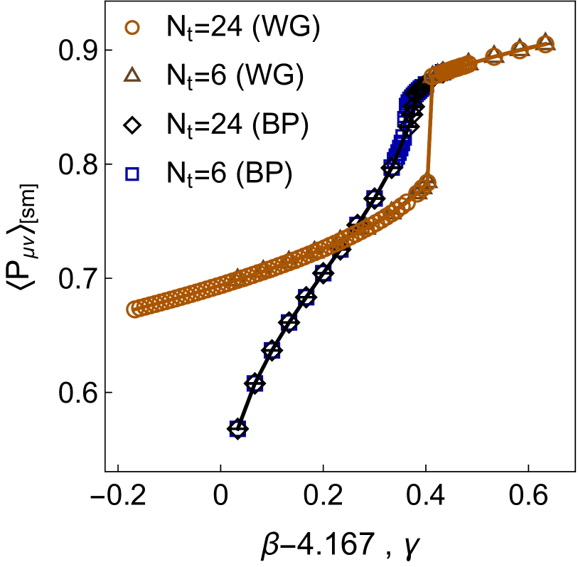
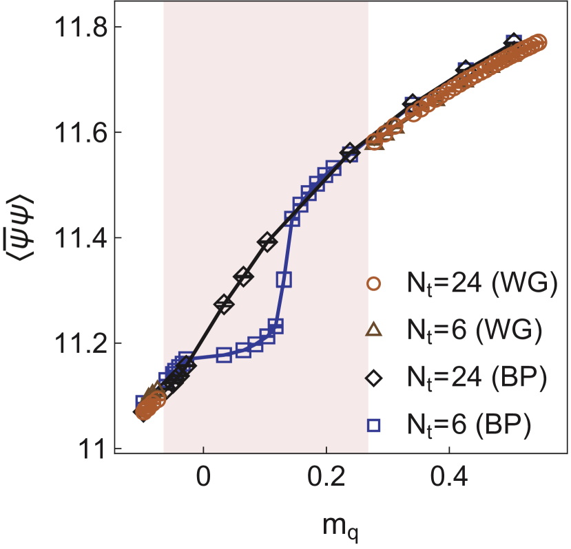
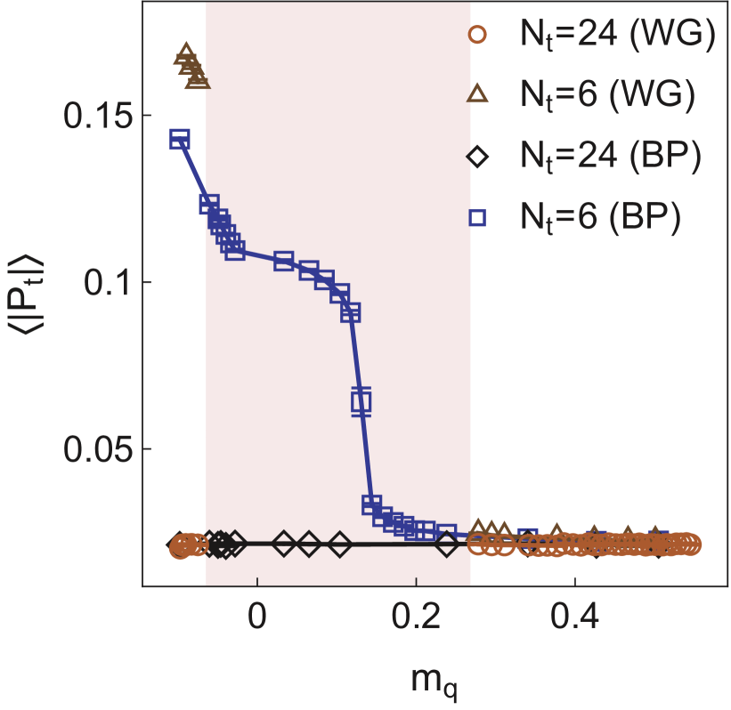
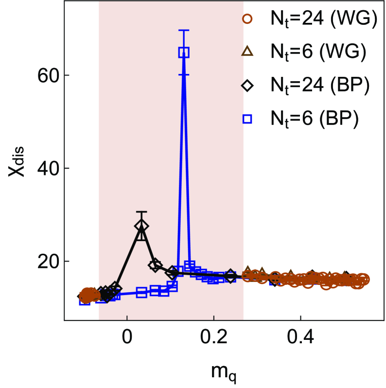
For values of above the line where the PCAC quark mass crosses zero coincides with the bulk transition line. Across these coinciding lines the system undergoes a first order transition and PCAC quark mass never passes through the value but jumps discontinuously from positive to negative values across the transition line. This is shown in the top left panel of Fig. 6 where the PCAC quark mass for the WG action (brown circles) is shown as function of at . To the left of the bulk transition line, the system is in the unphysical bulk phase, while to the right of the line the system has unphysical negative PCAC quark mass. Thus, the lattice does not describe any continuum-related physics for . Only for there is a range in for which the system is in the continuum phase and the PCAC quark mass is non-negative.
With , also the ”confinement/deconfinement” line in Fig. 5 is for on top of the bulk transition line. In the displayed range of the ”confinement/deconfinement” transition separates from the bulk transition line only for , but is then located in the negative PCAC mass region and hence unphysical. To extract information about the continuum theory form this lattice system, one would have to increase (and, correspondingly, also to avoid dominance of finite volume effects) so that the ”confinement/deconfinement” line fully separates from the bulk transition line. Thus, we can conclude that it is not possible to reach the light quark confinement (chiral) phase transition with the WG action using lattices. Of course, in the limit , where the quark mass grows much larger than the deconfinement energy scale, the ”confinement/deconfinement” line is expected to separate from the bulk transition line also for , as the fermions decouple and the system reduces to pure gauge .
Fig. 6 contains also results obtained with the bulk-preventing action (15). In this case the bulk transition is absent and the PCAC quark mass approaches continuously. The small gap in the data around is due to the slowing down caused by the appearance of zero eigenmodes of the Wilson-Dirac operator when . This could be avoided by e.g. using Schrödinger functional boundary conditions, which remove zero modes.
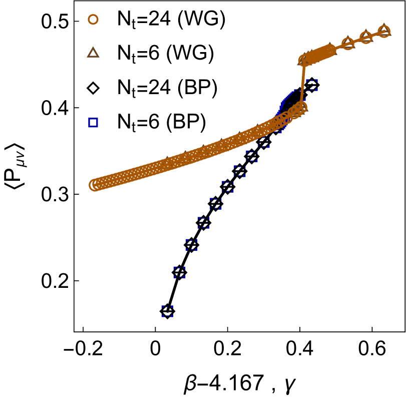
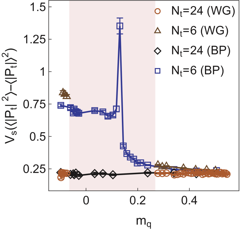
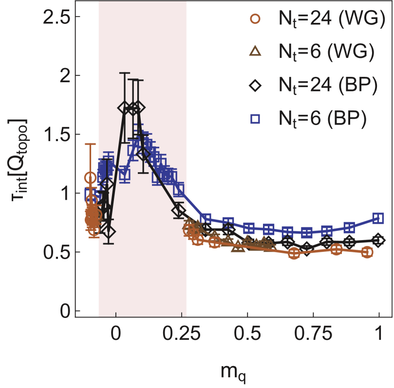
In the first two panels of the second and third row of Fig. 6 the chiral condensate (2nd row, left) and disconnected chiral susceptibility (last row, left), as well as the temporal Polyakov loop (2nd row, center) and corresponding variance (last row, center) are plotted as functions of the PCAC quark mass, . While deep in the strong-coupling and deep in the negative mass phase the results obtained with the WG action agree with those obtained using the BP action, the discontinuity in with the WG action (marked by the shaded areas) implies that the WG action cannot be used to study the transition region. On the other hand, with the BP action there is no discontinuity in and no bulk transition, and the behavior of the chiral condensate and the Polyakov loop at the finite-temperature phase transition are resolved.
The remaining two panels of Fig. 6, which show the topological susceptibility (2nd row, right) and integrated auto-correlation time for the topological charge itself (last row, right), indicate that also when coupled to fermions, fluctuations of the gauge-topology are not hindered by the use of the BP gauge action from (15) and HMC updates. For the values of which are accessible with both actions, both actions yield the same results for the topological susceptibility. The slightly higher integrated auto-correlation time for the topological charge with the BP action at is mostly due to a different tuning of the acceptance rates for the HMC trajectories.
IV Conclusions
We have identified a mechanism which appears to be relevant for the formation of unphysical ”bulk” configurations and the corresponding occurrence of a ”bulk transition” in simulations of lattice gauge theories using Wilson’s plaquette gauge action. We proposed a one-parameter family of alternative gauge actions, which possess the same continuum limit as the Wilson plaquette gauge action but which, when used in combination with an HMC update algorithm, prevent bulk-configurations from being created.
We tested our bulk-preventing simulation framework for pure gauge , pure gauge , and for with mass-degenerate Wilson-clover fermion flavors with hopping parameter , and which are coupled to the gauge field via 2-step stout smeared link variables. We found that in all three cases, the bulk-preventing action (15) with removes the bulk transition and reproduces at sufficiently weak coupling the same results as the Wilson plaquette action.
In the case of the fermionic theory, the Wilson gauge action could not be used to study the physical finite temperature phase transition on lattices at small quark masses. This is due to the fact that the bulk transition prevents the system from simultaneously reaching the physical transition region and small quark masses. On the other hand, with the bulk-preventing action (15) the bulk transition is absent and can be made arbitrarily small. It is also worth noting that the bulk-preventing actions do not seem to hinder any processes required for topology fluctuations.
Acknowledgements.
The authors acknowledge support from the Academy of Finland grants 308791, 319066, and 345070. T. R. is supported by the Swiss National Science Foundation (SNSF) through the grant no. TMPFP2_210064. The authors wish to acknowledge CSC - IT Center for Science, Finland, and the Finnish Computing Competence Infrastructure (FCCI) for computational resources.Appendix A Plaquette wrappings and magnetic monopole creation
In this appendix we discuss how in lattice gauge theory the plaquette wrapping types (a) and (b), introduced in Sec. II.1, are related to the creation of magnetic Dirac monopoles as defined in [33]. The situation with monopoles in lattice gauge theory will be addressed in the second part of this appendix.
A.1 Situation in
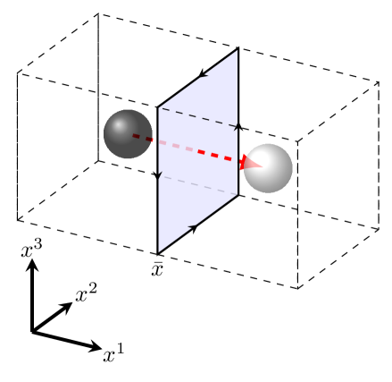
Dirac monopoles in lattice gauge theory, as described in [33], live on the dual lattice and are defined by a non-zero net physical magnetic flux through the boundary of a spatial cube. If this flux is non-zero for a given cube, then this cube contains a Dirac monopole. With our conventions, the corresponding operator can be written as:
| (20) |
which is the lattice analogue of the continuum expression, , with
| (21) |
i.e. . If one defines integer plaquette variables , so that
| (22) |
with from (8), then counts the amount of Dirac flux passing through the (oriented) plaquette on which is defined. The magnetic monopole operator (20) can then also be written as [33]
| (23) |
From (20) or (23) we see, that in order to produce or destroy a magnetic monopole, one has to change the net Dirac flux through the boundary of a spatial cube. Considering the plaquette wrapping types (a) and (b) introduced in Sec. II.1, a change of the net Dirac flux through the boundary of a spatial cube can only be achieved with plaquette wrappings of type (b). Fig. 7 illustrates how a type (b) plaquette wrapping of a spatial plaquette produces in the two adjacent spatial cubes a pair of magnetic monopoles of opposite charge. The monopoles serve, respectively, as source and sink for the Dirac flux passing through the wrapped plaquette.
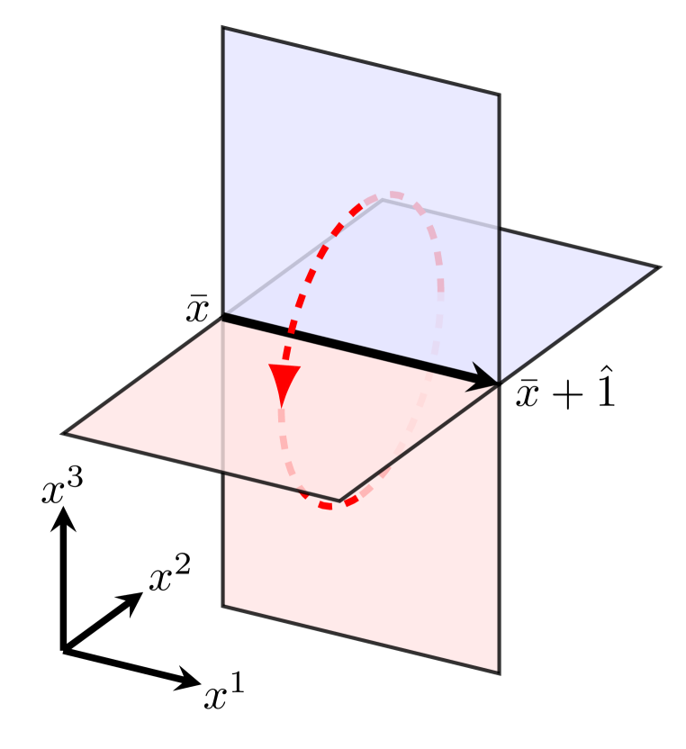
With plaquette wrappings of type (a) on the other hand, only closed Dirac strings can be produced and therefore no monopole/anti-monopole pairs are created. The reason for this is, that plaquette wrappings of type (a) are caused by a link variable wrapping around the -interval. Such a link wrapping will, however, never affect just a single plaquette but all plaquettes that contain the given link. If this link is a spatial one, it is contained in spatial as well as in temporal plaquettes. For the spatial plaquettes the wrapping creates the aforementioned Dirac flux that forms a closed loop winding around the shared link, illustrated in the left-hand panel of Fig. 8. For the temporal plaquettes, sketched in the right-hand panel of Fig. 8, the wrapping does not give rise to the production of Dirac flux as temporal plaquettes are associated to the electric and not the magnetic field. For the same reason, no Dirac flux is produced if the wrapping link is a temporal one, as this would affect only temporal plaquettes.
A.2 Situation in
In non-abelian gauge theory magnetic monopoles can be defined in different ways [34, 35, 36, 37] and can be divided into two categories: singular monopoles which require a Dirac string, and non-singular monopoles which possess a Dirac string only in certain gauges. On the lattice singular monopoles can be implemented in terms of net Dirac flux through the boundary of spatial cubes [38, 39, 40], with the Dirac flux, , , associated with a plaquette variable , being defined so that in the factorization
| (24) |
one has
| (25) |
The possible values for the first factor on the right-hand side of (24) correspond to the center of :
| (26) |
As the above discussed Dirac monopoles in lattice gauge theory, also the so defined monopoles decouple in the (naive) continuum limit of the lattice gauge theory. Preventing the formation of monopoles in lattice gauge theory (with WG action) has for been reported to push the bulk phase to stronger coupling [39]. Preventing not only monopoles but also the formation of Dirac strings from being formed removes the bulk phase completely [39, 22, 16]. The continuum limit of the model remains, however, unaffected by these modifications [41].
To make contact with our discussion in Sec. II.2 about the relation between the production of bulk configurations in lattice gauge theory and having plaquettes continuously crossing the cut locus of on , we note that the non-trivial center elements listed in (26) are all located beyond this cut locus for (resp. on the cut locus for ). Therefore, by preventing the continuous cut locus crossing of plaquettes, the production of Dirac flux though individual plaquettes is not possible, which should also prevent the production of monopole/anti-monopole pairs. This is the analogue of the type (b) plaquette wrapping from Sec. II.1, which is responsible for the monopole/anti-monopole pair production in lattice gauge theory, as described in Fig. 7.
We note that this does not imply that the use of our bulk-preventing actions (15) in combination with HMC updates would prevent the production of monopoles in general; only the production of cutoff scale monopoles is exlucded. Extended monpoles with ”thick” strings [42, 43, 44] attached should still be possible.
Also, the production of non-singular monopoles [45, 46] is not prevented by our bulk-preventing setup. Non-singular monopoles could on the lattice be located by gauge fixing the system to maximal abelian gauge (MAG) [47] and then performing abelian projection (AP) to the Cartan subgroup [48]. In each of the factors of one can then look for Dirac monopoles with the method from [33], discussed in the first part of this appendix. It is only in this maximum abelian gauge that non-singular monopoles show up as Dirac monopoles of the projected subgroup; fixing to another gauge before projecting to results in fewer monopoles being found [49] in the subgroup factors. We have not tried to use the MAG-AP method to monitor the monopole densities directly in our HMC simulations with the BP actions from (15). However, there is no reason to expect that the BP setup would prevent continuum-relevant monopoles from being produced. Since finite temperature instantons (calorons) can be described as composite objects, consisting of multiple monopoles [50], the bottom-left panels of Figs. 3,4, which illustrate that topology fluctuations are unhindered by the bulk-prevention, indicate that also the caloron constituent monopoles can fluctuate.
Appendix B Computing the gauge force
We note that the plaquette variables satisfy , so that also the from Eq. (16) satisfy . We can therefore write the bulk-preventing action from Eq. (15) as
| (27) |
Let us now denote by the variation with respect to the link-variable that lives on the link that points from site in -direction. We then have:
| (28) |
where
| (29) |
and we have used that as and commute with each other and with their inverses. If we now carry out the variation of the plaquette explicitly, we find:
| (30) |
where are the hermitian generators of , normalized so that . Plugging this into Eq. (28), we obtain after some manipulations:
| (31) |
with
| (32) |
being the plaquette that starts and ends at site and is spanned by the and the negative direction, and the corresponding A-matrix,
| (33) |
References
- [1] B. Lucini, M. Teper and U. Wenger, “Properties of the deconfining phase transition in SU(N) gauge theories,” JHEP 02 (2005), 033 doi:10.1088/1126-6708/2005/02/033 [arXiv:hep-lat/0502003 [hep-lat]].
- [2] A. Hasenfratz and T. A. DeGrand, “Heavy dynamical fermions in lattice QCD,” Phys. Rev. D 49 (1994), 466-473 doi:10.1103/PhysRevD.49.466 [arXiv:hep-lat/9304001 [hep-lat]].
- [3] F. Bursa, L. Del Debbio, L. Keegan, C. Pica and T. Pickup, “Mass anomalous dimension in SU(2) with six fundamental fermions,” Phys. Lett. B 696 (2011), 374-379 doi:10.1016/j.physletb.2010.12.050 [arXiv:1007.3067 [hep-ph]].
- [4] T. Karavirta, J. Rantaharju, K. Rummukainen and K. Tuominen, “Determining the conformal window: SU(2) gauge theory with = 4, 6 and 10 fermion flavours,” JHEP 05 (2012), 003 doi:10.1007/JHEP05(2012)003 [arXiv:1111.4104 [hep-lat]].
- [5] V. Leino, T. Rindlisbacher, K. Rummukainen, F. Sannino and K. Tuominen, “Safety versus triviality on the lattice,” Phys. Rev. D 101 (2020) no.7, 074508 doi:10.1103/PhysRevD.101.074508 [arXiv:1908.04605 [hep-lat]].
- [6] J. Rantaharju, T. Rindlisbacher, K. Rummukainen, A. Salami and K. Tuominen, “Spectrum of SU(2) gauge theory at large number of flavors,” Phys. Rev. D 104 (2021) no.11, 114504 doi:10.1103/PhysRevD.104.114504 [arXiv:2108.10630 [hep-lat]].
- [7] T. Rindlisbacher, K. Rummukainen, A. Salami and K. Tuominen, “Nonperturbative Decoupling of Massive Fermions,” Phys. Rev. Lett. 129 (2022) no.13, 131601 doi:10.1103/PhysRevLett.129.131601 [arXiv:2110.13882 [hep-lat]].
- [8] A. J. Hietanen, J. Rantaharju, K. Rummukainen and K. Tuominen, “Spectrum of SU(2) lattice gauge theory with two adjoint Dirac flavours,” JHEP 05 (2009), 025 doi:10.1088/1126-6708/2009/05/025 [arXiv:0812.1467 [hep-lat]].
- [9] F. Bursa, L. Del Debbio, L. Keegan, C. Pica and T. Pickup, “Mass anomalous dimension in SU(2) with two adjoint fermions,” Phys. Rev. D 81 (2010), 014505 doi:10.1103/PhysRevD.81.014505 [arXiv:0910.4535 [hep-ph]].
- [10] J. Rantaharju, “Gradient Flow Coupling in the SU(2) gauge theory with two adjoint fermions,” Phys. Rev. D 93 (2016) no.9, 094516 doi:10.1103/PhysRevD.93.094516 [arXiv:1512.02793 [hep-lat]].
- [11] T. Appelquist et al. [LSD], “Lattice simulations with eight flavors of domain wall fermions in SU(3) gauge theory,” Phys. Rev. D 90 (2014) no.11, 114502 doi:10.1103/PhysRevD.90.114502 [arXiv:1405.4752 [hep-lat]].
- [12] A. Hasenfratz, C. Rebbi and O. Witzel, “Gradient flow step-scaling function for SU(3) with Nf=8 fundamental flavors,” Phys. Rev. D 107 (2023) no.11, 114508 doi:10.1103/PhysRevD.107.114508 [arXiv:2210.16760 [hep-lat]].
- [13] T. Appelquist et al. [Lattice Strong Dynamics], “Nonperturbative investigations of SU(3) gauge theory with eight dynamical flavors,” Phys. Rev. D 99 (2019) no.1, 014509 doi:10.1103/PhysRevD.99.014509 [arXiv:1807.08411 [hep-lat]].
- [14] T. DeGrand, Y. Liu, E. T. Neil, Y. Shamir and B. Svetitsky, “Spectroscopy of SU(4) lattice gauge theory with fermions in the two index anti-symmetric representation,” PoS LATTICE2014 (2014), 275 doi:10.22323/1.214.0275 [arXiv:1412.4851 [hep-lat]].
- [15] T. DeGrand, Y. Shamir and B. Svetitsky, “Suppressing dislocations in normalized hypercubic smearing,” Phys. Rev. D 90 (2014) no.5, 054501 doi:10.1103/PhysRevD.90.054501 [arXiv:1407.4201 [hep-lat]].
- [16] V. G. Bornyakov, M. Creutz and V. K. Mitrjushkin, “Modified Wilson action and Z(2) artifacts in SU(2) lattice gauge theory,” Phys. Rev. D 44 (1991), 3918-3923 doi:10.1103/PhysRevD.44.3918
- [17] O. Akerlund and P. de Forcrand, “U(1) lattice gauge theory with a topological action,” JHEP 06 (2015), 183 doi:10.1007/JHEP06(2015)183 [arXiv:1505.02666 [hep-lat]].
- [18] D. Nogradi, L. Szikszai and Z. Varga, “Non-abelian lattice gauge theory with a topological action,” JHEP 08 (2018), 032 doi:10.1007/JHEP08(2018)032 [arXiv:1807.05295 [hep-lat]].
- [19] K. G. Wilson, “Confinement of Quarks,” Phys. Rev. D 10 (1974), 2445-2459 doi:10.1103/PhysRevD.10.2445
- [20] M. Luscher and P. Weisz, “On-Shell Improved Lattice Gauge Theories,” Commun. Math. Phys. 97 (1985), 59 [erratum: Commun. Math. Phys. 98 (1985), 433] doi:10.1007/BF01206178
- [21] W. Rossmann, “Lie Groups: An Introduction Through Linear Groups,” Oxford graduate texts in mathematics, 2002, Oxford University Press, isbn: 9780198596837.
- [22] R. C. Brower, D. A. Kessler and H. Levine, “The Onset of Asymptotically Free Scaling,” Phys. Rev. D 26 (1982), 959 doi:10.1103/PhysRevD.26.959
- [23] B. B. Brandt, R. Lohmayer and T. Wettig, “Induced QCD II: Numerical results,” JHEP 07 (2019), 043 doi:10.1007/JHEP07(2019)043 [arXiv:1904.04351 [hep-lat]].
- [24] G. Bhanot and M. Creutz, “Variant Actions and Phase Structure in Lattice Gauge Theory,” Phys. Rev. D 24 (1981), 3212 doi:10.1103/PhysRevD.24.3212
- [25] A. Hasenfratz, “Infrared fixed point of the 12-fermion SU(3) gauge model based on 2-lattice MCRG matching,” Phys. Rev. Lett. 108 (2012), 061601 doi:10.1103/PhysRevLett.108.061601 [arXiv:1106.5293 [hep-lat]].
- [26] M. Hasenbusch and S. Necco, “SU(3) lattice gauge theory with a mixed fundamental and adjoint plaquette action: Lattice artifacts,” JHEP 08 (2004), 005 doi:10.1088/1126-6708/2004/08/005 [arXiv:hep-lat/0405012 [hep-lat]].
- [27] W. Bietenholz, K. Jansen, K. I. Nagai, S. Necco, L. Scorzato and S. Shcheredin, “Exploring topology conserving gauge actions for lattice QCD,” JHEP 03 (2006), 017 doi:10.1088/1126-6708/2006/03/017 [arXiv:hep-lat/0511016 [hep-lat]].
- [28] T. DeGrand, “Simple chromatic properties of gradient flow,” Phys. Rev. D 95 (2017) no.11, 114512 doi:10.1103/PhysRevD.95.114512 [arXiv:1701.00793 [hep-lat]].
- [29] Z. Fodor, K. Holland, J. Kuti, D. Nogradi and C. H. Wong, “The Yang-Mills gradient flow in finite volume,” JHEP 11 (2012), 007 doi:10.1007/JHEP11(2012)007 [arXiv:1208.1051 [hep-lat]].
- [30] Z. Fodor, K. Holland, J. Kuti, S. Mondal, D. Nogradi and C. H. Wong, “The lattice gradient flow at tree-level and its improvement,” JHEP 09 (2014), 018 doi:10.1007/JHEP09(2014)018 [arXiv:1406.0827 [hep-lat]].
- [31] C. E. Detar, O. Kaczmarek, F. Karsch and E. Laermann, “String breaking in lattice quantum chromodynamics,” Phys. Rev. D 59 (1999), 031501 doi:10.1103/PhysRevD.59.031501 [arXiv:hep-lat/9808028 [hep-lat]].
- [32] F. Karsch, “Deconfinement and chiral symmetry restoration in QCD with fundamental and adjoint fermions,” PoS corfu98 (1998), 008 doi:10.22323/1.001.0008
- [33] T. A. DeGrand and D. Toussaint, “Topological Excitations and Monte Carlo Simulation of Abelian Gauge Theory,” Phys. Rev. D 22 (1980), 2478 doi:10.1103/PhysRevD.22.2478
- [34] P. Goddard and D. I. Olive, “New Developments in the Theory of Magnetic Monopoles,” Rept. Prog. Phys. 41 (1978), 1357 doi:10.1088/0034-4885/41/9/001
- [35] R. A. Brandt and F. Neri, “Magnetic Monopoles in SU(n) Gauge Theories,” Nucl. Phys. B 186 (1981), 84-108 doi:10.1016/0550-3213(81)90094-8
- [36] E. J. Weinberg, D. London and J. L. Rosner, “Magnetic Monopoles With ) Charges,” Nucl. Phys. B 236 (1984), 90-108 doi:10.1016/0550-3213(84)90526-1
- [37] S. Hollands and M. Muller-Preussker, “Definition of magnetic monopole numbers for SU(N) lattice gauge Higgs models,” Phys. Rev. D 63 (2001), 094503 doi:10.1103/PhysRevD.63.094503 [arXiv:hep-th/9901114 [hep-th]].
- [38] A. Ukawa, P. Windey and A. H. Guth, “Dual Variables for Lattice Gauge Theories and the Phase Structure of Z(N) Systems,” Phys. Rev. D 21 (1980), 1013 doi:10.1103/PhysRevD.21.1013
- [39] R. C. Brower, D. A. Kessler and H. Levine, “Monopole Condensation and the Lattice QCD Crossover,” Phys. Rev. Lett. 47 (1981), 621 doi:10.1103/PhysRevLett.47.621
- [40] P. de Forcrand, C. Korthals-Altes and O. Philipsen, “Screening of Z(N) monopole pairs in gauge theories,” Nucl. Phys. B 742 (2006), 124-141 doi:10.1016/j.nuclphysb.2006.02.035 [arXiv:hep-ph/0510140 [hep-ph]].
- [41] J. Fingberg, U. M. Heller and V. K. Mitrjushkin, “Scaling in the positive plaquette model and universality in SU(2) lattice gauge theory,” Nucl. Phys. B 435 (1995), 311-338 doi:10.1016/0550-3213(94)00492-W [arXiv:hep-lat/9407011 [hep-lat]].
- [42] G. Mack and V. B. Petkova, “Comparison of Lattice Gauge Theories with Gauge Groups Z(2) and SU(2),” Annals Phys. 123 (1979), 442 doi:10.1016/0003-4916(79)90346-4
- [43] G. Mack and V. B. Petkova, “Sufficient Condition for Confinement of Static Quarks by a Vortex Condensation Mechanism,” Annals Phys. 125 (1980), 117 doi:10.1016/0003-4916(80)90121-9
- [44] R. C. Brower, D. A. Kessler and H. Levine, “Dynamics of SU(2) Lattice Gauge Theories,” Nucl. Phys. B 205 (1982), 77 doi:10.1016/0550-3213(82)90467-9
- [45] G. ’t Hooft, “Magnetic Monopoles in Unified Gauge Theories,” Nucl. Phys. B 79 (1974), 276-284 doi:10.1016/0550-3213(74)90486-6
- [46] A. M. Polyakov, “Particle Spectrum in Quantum Field Theory,” JETP Lett. 20 (1974), 194-195 PRINT-74-1566 (LANDAU-INST).
- [47] C. Bonati and M. D’Elia, “The Maximal Abelian Gauge in SU(N) gauge theories and thermal monopoles for N = 3,” Nucl. Phys. B 877 (2013), 233-259 doi:10.1016/j.nuclphysb.2013.10.004 [arXiv:1308.0302 [hep-lat]].
- [48] G. ’t Hooft, “Topology of the Gauge Condition and New Confinement Phases in Nonabelian Gauge Theories,” Nucl. Phys. B 190 (1981), 455-478 doi:10.1016/0550-3213(81)90442-9
- [49] C. Bonati, A. Di Giacomo and M. D’Elia, “Detecting monopoles on the lattice,” Phys. Rev. D 82 (2010), 094509 doi:10.1103/PhysRevD.82.094509 [arXiv:1009.2425 [hep-lat]].
- [50] K. M. Lee and C. h. Lu, “SU(2) calorons and magnetic monopoles,” Phys. Rev. D 58 (1998), 025011 doi:10.1103/PhysRevD.58.025011 [arXiv:hep-th/9802108 [hep-th]].