Regularization of the ensemble Kalman filter using a non-stationary spatial convolution model

Abstract

Applications of the ensemble Kalman filter to high-dimensional problems are feasible only with small ensembles. This necessitates a kind of regularization of the analysis (observation update) problem. We propose a regularization technique based on a new non-stationary, non-parametric spatial model on the sphere. The model termed the Locally Stationary Convolution Model is a constrained version of the general Gaussian process convolution model. The constraints on the location-dependent convolution kernel include local isotropy, positive definiteness as a function of distance, and smoothness as a function of location. The model allows for a rigorous definition of the local spectrum, which is required to be a smooth function of spatial wavenumber. We propose and test an ensemble filter in which prior covariances are postulated to obey the Locally Stationary Convolution Model. The model is estimated online in a two-stage procedure. First, ensemble perturbations are bandpass filtered in several wavenumber bands to extract aggregated local spatial spectra. Second, a neural network recovers the local spectra from sample variances of the filtered fields. In simulation experiments, the new filter was capable of outperforming several existing techniques. With small to moderate ensemble sizes, the improvement was substantial.

Keywords: Process convolution model, Spatial non-stationarity, Data assimilation, Ensemble Kalman Filter, Neural network.

1 Introduction

Modern data assimilation relies on the ensemble technique, in which the probability distribution of the unknown system state is represented by a finite sample (ensemble) of pseudo-random realizations (ensemble members). This allows for realistic, spatially varying prior covariances in the analysis (the observation update step of the data assimilation cycle). In practical applications, the most widely-used approach is the Ensemble Kalman Filter (EnKF) and its numerous modifications and extensions. The principal problem of the ensemble approach is that running many ensemble members is computationally expensive. For real-world high-dimensional systems with billions of degrees of freedom, this means that only small ensembles (normally, comprising just tens of members) are affordable. As a result, such ensembles can provide the analysis with only scarce information on the prior distribution. The sample covariance matrix is a poor estimate of the true covariance matrix if the sample size is much lower than the dimensionality of the state space. This requires a kind of regularization, that is, the introduction of additional information on prior covariances. The following approaches have been proposed so far.

1. The most popular approach is covariance localization (tapering), [e.g. 11, 19], which reduces spurious long-distance correlations through element-wise multiplication of the sample covariance matrix by an ad-hoc positive definite localization matrix. This technique efficiently removes a lot of noise in the sample covariance matrix. But it cannot cope with the noise at small distances, it inevitably leads to an underestimation of the assumed length scale of the forecast-error field, and it can also destroy balances between different fields [19].

2. Blending sample covariances with static (time-mean) covariances is widely used in meteorological ensemble-variational schemes [7, 28]. In statistical literature, similar techniques are known as shrinkage estimators [24]. Sample covariances are noisy but they do contain the useful flow-dependent “signal”. Static covariances are noise-free but can be irrelevant under some flow conditions and observation coverage. A convex combination of the two covariance matrices proved to be useful (see the above references) but it is not selective: the noise in the sample covariances is reduced to the same extent as the flow-dependent non-stationary signal.

3. Another approach is spatial averaging of sample covariances (that is, blending with neighboring in space covariances) [e.g. 2]. The technique reduces noise in sample covariances due to an increase in the effective ensemble size but it does so at the expense of somewhat distorting (smoothing) the covariances. Optimal linear filtering of sample covariances [31] further develops this idea.

4. A similar technique is temporal averaging of sample covariances (i.e., blending with recent past covariances). Berre et al. [3], Bonavita et al. [4] used prior ensembles from several previous assimilation cycles to increase the ensemble size. Lorenc [27] used time-shifted ensemble perturbations for the same purpose. Tsyrulnikov and Rakitko [41] arrived at this technique by assuming that the true covariance matrix is an unknown random matrix and introducing a secondary filter in which the covariances are updated.

5. [44] proposed to regularize the sample covariance matrix by imposing a sparse structure in the inverse covariance (precision) matrix. A similar approach was taken by Hou et al. [18]. Gryvill and Tjelmeland [15] imposed a Markov random field structure to obtain a sparse prior precision matrix. Boyles and Katzfuss [5] postulated sparsity in inverse Cholesky factors of the prior covariance matrix.

6. One more option is to adopt a parametric forecast-error covariance model and estimate parameters of the model from the forecast ensemble. Skauvold and Eidsvik [37] used maximum likelihood estimates of a few model parameters in stationary and non-stationary settings.

7. Finally, imposing a structure in wavelet space can be used to regularize the analysis. Postulating the simplest structure, the diagonal wavelet covariance matrix, proved to be effective in data assimilation applications [10, 32], see also Kasanickỳ et al. [21]. This indicates that the regularizing effect of that approach can outweigh methodological errors related to the neglect of off-diagonal covariances in wavelet space.

In this paper, we propose to regularize the analysis problem by imposing a spatial model. In this regard, our approach is similar to the two latter techniques (items 6 and 7). In contrast to parametric covariance models, we aim at a non-parametric formulation to obtain a more flexible model. By non-parametric, we mean defined by parameters whose number is not fixed (as with a parametric model) but grows with the growing spatial resolution of the model. As compared with wavelet-diagonal models, which provide regularizing information by imposing zero correlations in wavelet space, our model does so by imposing several constraints on the general process convolution model. The principal constraint is local stationarity, by which we mean the capability of being approximated by a stationary model locally in space.

In section 2 we introduce a non-parametric locally stationary Gaussian process convolution model on the sphere (and on the circle). In section 3 we present a computationally efficient estimator of the model from an ensemble of random field realizations. Section 4 describes how the spatial model is used to regularize the analysis step of the new Locally Stationary convolutional Ensemble Filter (LSEF). We test the new approach in numerical experiments with a non-stationary random field model on the sphere (section 5) and in cyclic filtering on the circle (section 6).

Reproducible python and R code for numerical experiments presented in this paper can be found at https://github.com/Arseniy100/LSEF.

2 Spatial model

As noted in the Introduction, we employ a non-parametric spatial model for the forecast-error random field to regularize the data assimilation problem. Following [17], we rely on the Gaussian process convolution model. In contrast to most applications, which postulate a parametric model for the spatial convolution kernel (e.g., Lemos and Sansó [25], Sham Bhat et al. [36], Heaton et al. [16], Li and Zhu [26]), we choose a non-parametric approach to allow for variable shapes of spatial covariances. Non-parametric convolution kernels were considered by Tobar et al. [39], Bruinsma et al. [6] in the stationary time series context. Here we propose a non-parametric non-stationary spatial convolution model on compact manifolds such as the sphere and the circle.

The default domain is the two-dimensional unit sphere ${\mathbb{S}}^{2}$ (the domain of interest in geosciences) and on the unit circle ${\mathbb{S}}^{1}$ (used as a much simpler analog of the spherical case). We refer to ${\mathbb{S}}^{2}$ and ${\mathbb{S}}^{1}$ just as the sphere and the circle in the sequel. We denote points on the sphere as $x,y,\dots$ and area elements simply by ${\rm d}x,{\rm d}y,\dots$. On the sphere, we use the terms stationarity and isotropy interchangeably. We confine ourselves to band-limited functions because, in practice, fields to be estimated from observations inevitably have limited spatial resolution.

2.1 General process convolution model

Let $\xi(x)$ (where $x$ is the spatial coordinate) be a general real-valued space-continuous zero-mean linear Gaussian process, that is, the process whose values are linear combinations of the real-valued white Gaussian noise $\alpha(y)$:

$$\xi(x)=\int_{D}w(x,y)\,\alpha(y)\,{\rm d}y\equiv\int_{D}w(x,y)\,Z({\rm d}y).$$ (1)

Here $D$ is the domain of interest, $Z$ is the Gaussian orthogonal stochastic measure such that $\operatorname{\mathbb{E}}Z({\rm d}A)=0$, $\operatorname{\mathbb{E}}(Z({\rm d}A))^{2}=|{\rm d}A|$, and $\operatorname{\mathbb{E}}Z({\rm d}A)Z({\rm d}B)=0$ whenever ${\rm d}A\cap{\rm d}B=\emptyset$, ${\rm d}A$ is an area element, $|{\rm d}A|$ its surface area, $\operatorname{\mathbb{E}}$ is expectation, and $w(x,y)$ is a real function called the convolution kernel. In theoretical statistics, processes defined by Eq.(1) are sometimes called of Karhunen class [20].

The (non-stationary in general) covariance function of the process $\xi(x)$ defined by Eq.(1) is $B(x,x^{\prime})=\operatorname{\mathbb{E}}\xi(x)\xi(x^{\prime})=\int w(x,y)w(x^{\prime},y)\,{\rm d}y.$ Technically, this equation implies that for ${\mathsf{Var}}\,\xi(x)$ to be finite, the kernel $w(x,y)$ needs to be square integrable w.r.t. its second argument for any $x$: $\int w^{2}(x,y)\,{\rm d}y<\infty$.

Rather than using the kernel $w$ that depends on two points in the domain, $(x,y)$, we wish to work with a kernel, $v$, that depends on the point $x$ and on the relative location, let it be called $z$, of the point $y$ w.r.t. $x$. This is most easily done in the circular case, where we define $z=y-x$ (“distance with the sign”) and $v(x,z)=w(x,x+z)$. As a result, we can rewrite Eq.(1) as

$$\xi(x)=\int_{{\mathbb{S}}^{1}}w(x,y)\,\alpha(y)\,{\rm d}y\equiv\int_{{\mathbb{S}}^{1}}v(x,z)\,\alpha(x+z)\,{\rm d}z.$$ (2)

The new kernel $v(x,z)$ can be viewed as a spatially varying (with $x$) convolution kernel w.r.t. $z$. If $v(x,z)$ is independent of $x$, Eq.(2) becomes the ordinary convolution and $\xi$ becomes a stationary random process.

On the sphere, the definition of $v(x,z)$ is a bit more complicated because we cannot add and subtract points on the sphere. To proceed, we note that, still on the circle, Eq.(2) can be rewritten using rotations of the coordinate system. Specifically, for any $x$, let us rotate (counter-clockwise) the coordinate system by the angle $x$. Denoting the respective (orthogonal) change-of-basis matrix by ${\cal R}_{x}$, we realize that the point whose coordinates were $y$ in the unrotated system will have coordinates $z={\cal R}_{x}^{-1}y=y-x$ in the rotated system. Thus we can rewrite Eq.(2) as

$$\xi(x)=\int v(x,{\cal R}_{x}^{-1}y)\,\alpha(y)\,{\rm d}y=\int v(x,z)\,\alpha({\cal R}_{x}z)\,{\rm d}z.$$ (3)

Now, we note that this equation is applicable to the spherical domain as well. To see this, we consider a coordinate system’s rotation that takes the North Pole to the point $x$ and let ${\cal R}_{x}$ be the associated change-of-basis matrix. Denoting

$$v(x,z)=w(x,{\cal R}_{x}z)$$ (4)

and changing variables in the integral $\int w(x,y)\,\alpha(y)\,{\rm d}y$ in Eq.(1) from $y$ to $z={\cal R}_{x}^{-1}y$ while utilizing orthogonality of ${\cal R}_{x}$, we obtain Eq.(3).

2.2 Constraining the model: strategy

In the formulations Eq.(1) and (3), however, the model is not identifiable, that is, the function $w(x,y)$ is not unique given the process covariance function $B(x,x^{\prime})$. Indeed, consider an isotropic convolution kernel $\psi(\rho(y,y^{\prime}))$ (where $\rho(y,y^{\prime})$ stands for the great-circle distance between the points $y$ and $y^{\prime}$) whose Fourier transform (on ${\mathbb{S}}^{1}$) or Fourier-Legendre transform (on ${\mathbb{S}}^{2}$) is equal to one in modulus (see Appendix A for the definition of the Fourier-Legendre transform we use). Then, it is straightforward to see that the covariance function remains unchanged if $w(x,y)$ is convolved with $\psi$. (The convolution with such a kernel is analogous to the multiplication by an orthogonal matrix in the space discrete case.)

We intend to introduce constraints on the convolution kernel aimed to make the model identifiable and to reduce the effective number of degrees of freedom in the model, thus facilitating its estimation from a small ensemble of random field realizations.

2.3 Locally isotropic kernel

The first constraint we impose on the convolution kernel $w(x,y)$ requires that for any $x$, the function $v(x,z)=w(x,{\cal R}_{x}z)$ depends only on the co-latitude of $z$, that is, on the distance between $x$ and $y={\cal R}_{x}z$. So, there is a real-valued function $u(x,\rho(x,y))$ such that

$$w(x,y)=u(x,\rho(x,y)).$$ (5)

Substituting Eq.(5) into Eq.(1) yields

$$\xi(x)=\int u(x,\rho(x,y))\,\alpha(y)\,{\rm d}y.$$ (6)

In the remainder of this subsection, we develop spectral representations of the process defined by Eq.(6) and of its spatial covariances. We perform the spectral (Fourier-Legendre) expansion (Appendix A) of $u(x,\rho)$ with $x$ being fixed:

$$u(x,\rho)=\sum^{\ell_{\rm max}}_{\ell=0}\frac{2\ell+1}{4\pi}\sigma_{\ell}(x)P_{\ell}(\cos\rho),$$ (7)

where $P_{\ell}$ is the Legendre polynomial. Substituting $\rho=\rho(x,y)$ into Eq.(7) and applying the addition theorem for spherical harmonics (see again Appendix A), we obtain

$$u(x,\rho(x,y))=\sum^{\ell_{\rm max}}_{\ell=0}\sigma_{\ell}(x)\sum^{\ell}_{m=-\ell}Y_{\ell m}(x)\,Y_{\ell m}^{*}(y).$$ (8)

Then, we write down the spectral expansion of the band-limited Gaussian white noise:

$$\alpha(y)=\sum^{\ell_{\rm max}}_{\ell=0}\sum^{\ell}_{m=-\ell}\widetilde{\alpha}_{\ell m}\,Y_{\ell m}(y).$$ (9)

Here $\widetilde{\alpha}_{\ell m}$ are mutually uncorrelated complex-valued random Fourier coefficients with $\operatorname{\mathbb{E}}\widetilde{\alpha}_{\ell m}=0$ and ${\mathsf{Var}}\,\widetilde{\alpha}_{\ell m}=1$. More specifically, $\widetilde{\alpha}_{l0}$ are real valued and all the other $\widetilde{\alpha}_{\ell m}$ are complex circularly symmetric random variables [e.g. 35, section 9.5] such that $\widetilde{\alpha}_{l,-m}=\widetilde{\alpha}_{\ell m}^{*}$.

Finally, we substitute Eqs. (9) and (8) into Eq.(6). Utilizing the orthonormality of spherical harmonics, we obtain the basic spectral representation of the random process that satisfies Eq.(6):

$$\xi(x)=\sum^{\ell_{\rm max}}_{\ell=0}\sum^{\ell}_{m=-\ell}\sigma_{\ell}(x)\,\widetilde{\alpha}_{\ell m}\,Y_{\ell m}(x).$$ (10)

Note that from Eq.(7) it follows that $\sigma_{\ell}(x)$ (we call them the spectral functions) are real valued. The spatial covariances can readily be obtained from Eq.(10) by taking into account that all $\widetilde{\alpha}_{\ell m}$ are mutually uncorrelated and again applying the addition theorem for spherical harmonics:

$$B(x,x^{\prime})=\operatorname{\mathbb{E}}\xi(x)\xi(x^{\prime})=\sum^{\ell_{\rm max}}_{\ell=0}\frac{2\ell+1}{4\pi}\,\sigma_{\ell}(x)\,\sigma_{\ell}(x^{\prime})\,P_{\ell}(\cos\rho(x,x^{\prime})).$$ (11)

If $u(x,\rho)=u(\rho)$ or, equivalently, if all spectral functions $\sigma_{\ell}(x)$ do not depend on $x$, then the model Eq.(6) or Eq.(10) becomes a stationary (isotropic) random field model. Equation (11) shows that the process variance ${\mathsf{Var}}\,\xi(x)$ can be obtained by summing $\frac{2\ell+1}{4\pi}f_{\ell}(x)$ known in the stationary case as the variance spectrum (energy per degree $\ell$). Again in the stationary case, $f_{\ell}$ are often called the modal spectrum (energy per ‘mode”, i.e., per pair $(\ell,m)$). In the non-stationary case, in which $f_{\ell}$ depend on $x$, we call $f_{\ell}(x)$ the local modal spectrum or just the local spectrum.

The formulation of the spatial model Eq.(10) on the circle is outlined in Appendix B.

2.4 Positive definite convolution kernel

In Appendix D we consider the process $\xi_{\rm statio}$ defined by the process convolution model with the stationary kernel $u(\rho)$, see Eq.(40). As discussed above, the kernel is not unique given the covariance function of the process. In an attempt to select a unique kernel, we impose a computationally motivated spatial localization requirement, seeking $u(\rho)$ that has the smallest spatial scale. We show that there are three solutions to this optimization problem, all of them having the same shape of the kernel. One of these three equivalent solutions is positive definite, which we select. A similar result is valid for the process defined on the circle. So, with a stationary process defined by the convolution $\xi=u*\alpha$ (where $\alpha$ is the white noise) and having a given spatial covariance function, the most spatially localized kernel $u$ can be considered to be a positive definite function of distance.

Motivated by this result, we postulate that in the non-stationary case, for any $x$, the kernel $u(x,\rho)$ is a positive definite function of distance $\rho$. As a consequence, $\sigma_{\ell}(x)>0$ both in the spherical and in the circular case. This constitutes our second constraint imposed on the general process convolution model.

In Appendix C we prove that the local isotropy constraint, section 2.3, and the positive-definiteness constraint, section 2.4, guarantee (with some technical assumption) that the kernel $u(x,\rho)$ can be uniquely determined from the model’s non-stationary covariances $B(x,x^{\prime})$.

To further reduce the effective number of degrees of freedom, we introduce two additional regularizing constraints. These are smoothness constraints, one imposed in physical space and the other in spectral space.

2.5 Local stationarity

The model formulation based on the locally isotropic convolution kernel $u(x,\rho(x,y))$, Eq.(6), (or on the kernel $v(x,z)$, Eq.(3)) enables us to introduce two spatial scales. The first one is the length scale at which $u(x,\rho)$ typically varies as a function of distance $\rho$. We call it the characteristic length scale $L$ of the process $\xi(x)$ (defined in Appendix E). The other one is the length scale at which $u(x,\rho)$ varies as a function of location $x$. We refer to it as the non-stationarity length scale $\Lambda$ also introduced in Appendix E, where we show that the process $\xi(x)$ is locally stationary if one of the following two conditions are met.

The first condition is $L\ll\Lambda$, that is, the requirement that the local structure of the process changes in space on a scale much larger than the length scale of the process itself. The second condition is that the spatial variability in the convolution kernel (measured by a non-stationarity strength, see Appendix E) is small. In this case the process is locally stationary even if $\Lambda$ is comparable with $L$.

These conditions are obtained in Appendix E under the assumption that the local spectra $f_{0}(x),f_{1}(x),\dots,f_{\ell_{\rm max}}(x)$ are a stationary vector-valued random process of location $x$ and considering the conditional distribution of the process $\xi$ given its local spectra. Equivalently, conditioning on the convolution kernel $u(x,\rho)$ (viewed as a Hilbert space valued stationary random process of $x$) can be considered.

Local stationarity is the third constraint we introduce. Note that the slow variation of the kernel $u(x,\rho)$ with location $x$ (as compared to its variation as a function of distance $\rho$), actually, justifies the above term “local spectrum” introduced first in the time series context by Priestley [34], who called it evolutionary spectrum.

2.6 Smoothness of local spectra

Studies of real-world spatio-temporal processes showed that spatial (and temporal) spectra in turbulent flows are quite smooth, exhibiting typically a power-law behavior at large wavenumbers, e.g., Gage and Nastrom [12], Trenberth and Solomon [40]. For this reason and to regularize the spatial model by further reducing its effective number of degrees of freedom, we postulate that the local spatial spectra $f_{\ell}(x)$ are smooth functions of the wavenumber $\ell$ — this is our fourth constraint. Note that a smooth local spectrum $f_{\ell}(x)$ corresponds to the rapidly decreasing kernel $u(x,\rho)$ with distance $\rho$.

2.7 Summary of constraints

1. The convolution kernel has the locally isotropic form $w(x,y)=u(x,\rho(x,y))$.

2. The convolution kernel $u(x,\rho)$ is a positive definite function of distance $\rho$.

3. The process $\xi(x)$ is locally stationary.

4. The local spatial spectra $f_{\ell}(x)$ are smooth functions of the wavenumber $\ell$.

Below we refer to the above spatial model that obeys these four constraints as the Locally Stationary Convolution Model.

3 Estimation of the model from the ensemble

In this section, we propose an estimator of the Locally Stationary Convolution Model from an ensemble (sample) of $n_{\rm e}$ independent identically distributed random field realizations: $\{\xi^{(k)}(x)\}_{k=1}^{n_{\rm e}}$. The goal is to estimate the convolution kernel $u(x,\rho(x,y))$. Recall that for any $x$, the convolution kernel $u(x,\rho(x,y))$ is the inverse Fourier-Legendre transform of the spectral functions $\sigma_{\ell}(x)=\sqrt{f_{\ell}(x)}$ (see Eq.(7)), so it suffices to estimate the local spectra $f_{\ell}(x)$. The estimator should be applicable to high-dimensional problems.

We note that the exact likelihood of the data $\xi^{(.)}(.)$ generated by the model Eq.(10) given the spectral functions $\sigma_{.}(.)$ is computationally intractable. To arrive at an estimator affordable in very high dimensions, we make a few approximations. As a result, we obtain a two-stage estimator. First, a number of bandpass filters are applied to the input ensemble and sample variances of their outputs are computed. Second, the local spectra $f_{\ell}(x)$ are restored from those sample variances.

Our approach can be regarded as a modification of the technique by Priestley [34], who, for each frequency $\omega_{0}$, applied a narrow bandpass filter centered at $\omega_{0}$ to a non-stationary time series and used the filter’s mean-squared output as the estimate of his evolutionary spectrum at the same frequency. Another relevant reference is Marinucci and Peccati [30, chapter 11], who applied a wavelet filter to extract the variance spectrum of an isotropic random field on the sphere.

3.1 Multiple spatial bandpass filters

In the stationary case, it is straightforward to derive from Eq.(38) that the likelihood of the data, i.e., the ensemble of random-field realizations $\{\xi^{(k)}(x)\}_{k=1}^{n_{\rm e}}$, given the spectrum $\{f_{\ell}\}_{\ell=0}^{\ell_{\rm max}}$ depends on the data through the set of single-wavenumber sample variances $\widehat{v}_{\ell}=\frac{1}{n_{\rm e}}\sum_{k=1}^{n_{\rm e}}\sum_{m=-\ell}^{\ell}|\widetilde{\xi}_{\ell m}^{(k)}|^{2}$. (Note that with $n_{\rm e}=1$, the set of $\widehat{v}_{\ell}$ is the spherical analog of what is known in the time series context as the periodogram.) Therefore, the vector of the single-wavenumber sample variances $\widehat{v}_{\ell}$ (with $\ell=0,1,\dots,\ell_{\rm max}$) is a sufficient statistic for the spectrum $f_{\ell}$. This implies that no information on the true spectrum is lost if we switch from the raw ensemble to the set of $\widehat{v}_{\ell}$.

In the locally stationary case, however, relying on the single-wavenumber sample variances is not a good idea because isotropic spatial filters that isolate individual spectral components have non-local impulse response functions. Indeed, the filter, ${\cal H}$, whose spectral transfer function $H(\ell)$ is equal to one at $\ell_{0}$ and zero otherwise, has the response function $h(\rho(x,y))=\frac{2\ell_{0}+1}{4\pi}P_{\ell_{0}}(cos(\rho(x,y)))$ (see Eq.(28)). Due to the non-locality of $P_{\ell_{0}}(cos(\rho))$, the filtered signal, which is the convolution of the input signal with $h(\rho(x,y)$, will contain significant contributions from over the whole global domain. This is not acceptable in the non-stationary case, in which we seek primarily local contributions.

To localize $h(\rho)$, we specify a broader $H(\ell)$. Broadening the filter’s transfer functions reduces the spectral resolution of the estimator. To retain some spectral resolution, we require that the width $d$ of the filter’s transfer function is much less than the width of the mean spectrum of $\xi(x)$, or, equivalently (see Eq.(44)), $L\ll L_{\cal H}$, where $L_{\cal H}=1/d$ is the width of the filter’s impulse response function and $L$ is defined in Appendix E. According to our fourth constraint (section 2.7), the spatial spectra are smooth, so high spectral resolution is not needed. The optimal trade-off between spatial and spectral localization was established in this study empirically.

Technically, we performed bandpass filtering of the non-stationary process that satisfies Eq.(10) using $J$ filters ${\cal H}_{j}$, where $j=1,\dots,J$. The spectral transfer functions were specified as

$$H_{j}(\ell)=\exp\left(-\left|\frac{\ell-\ell^{\rm c}_{j}}{d_{j}}\right|^{q_{\rm shape}}\right),$$ (12)

where $\ell^{\rm c}_{j}$ is the central wavenumber of the $j$th filter, ${d_{j}}$ is its half-width, and $q_{\rm shape}$ is the shape parameter. In the experiments described below, we took ${q_{\rm shape}}$ equal to 3 (${q_{\rm shape}}=2$ also worked well). Both $\ell^{\rm c}_{j}$ and ${d_{j}}$ were taken exponentially growing with the band index $j$. Figure 1 shows an example of spectral transfer functions and the respective impulse response functions for six bandpass filters used in the experiments presented in section 5. The spatial filtering was performed in spectral space.

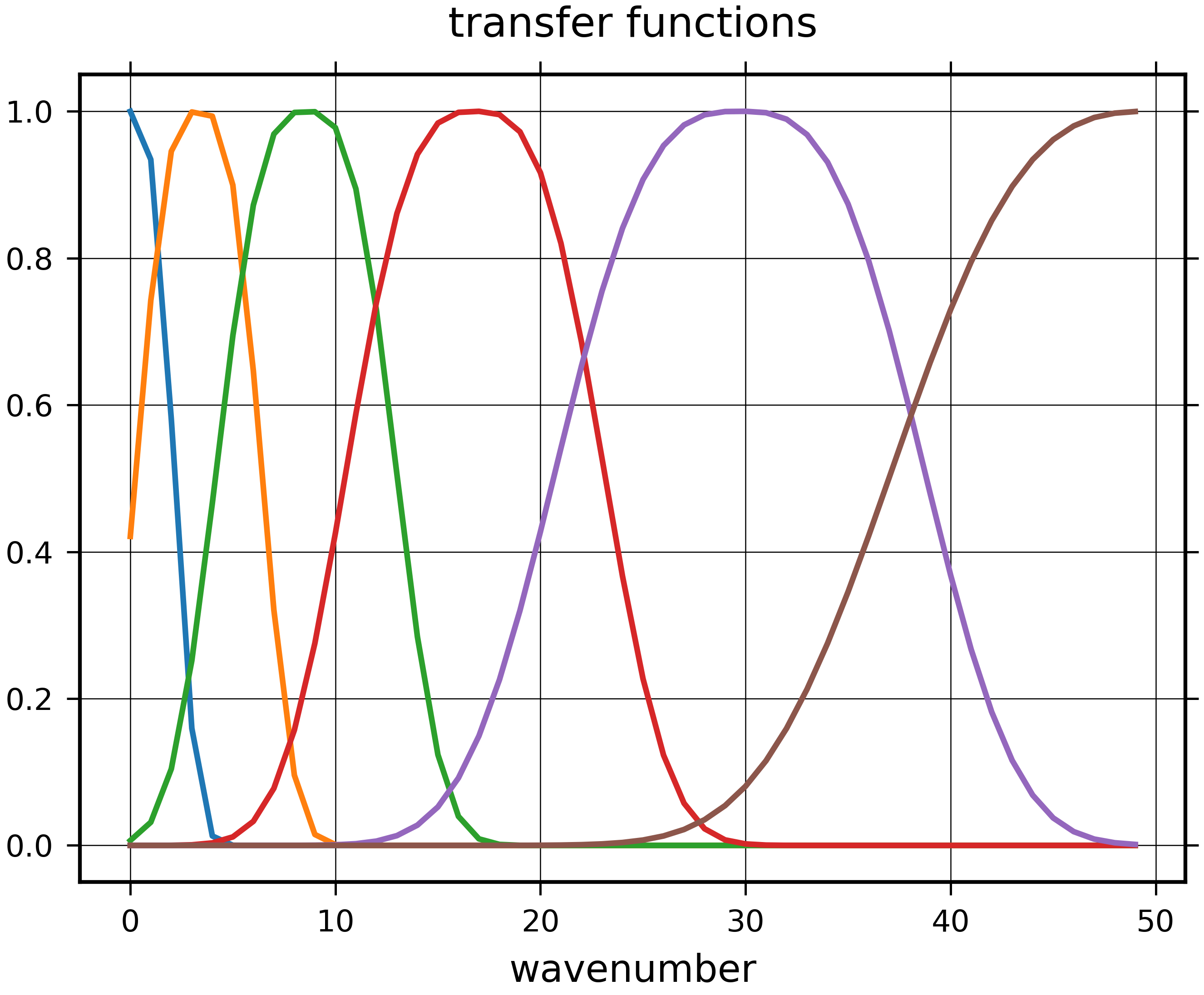
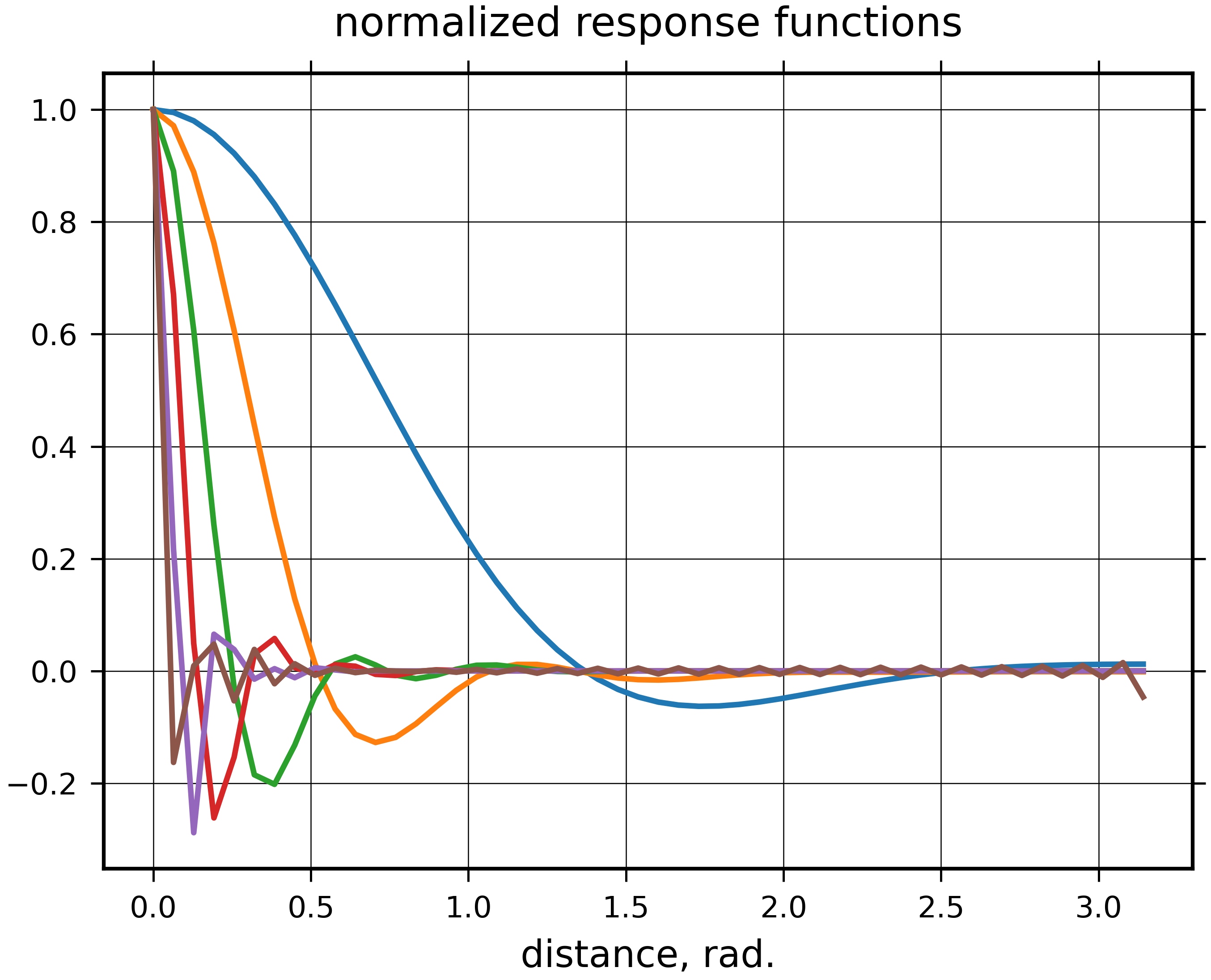
Figure 1: Spectral transfer functions $H_{j}(\ell)$ (left) and their respective normalized impulse response functions $h_{j}(\rho)$ (right) for six bandpass filters.

3.2 Sample band variances

As discussed in the previous subsection, to obtain some spatial resolution in the local spectra $\sigma_{\ell}(x)$ we seek to estimate, we have to reduce the spectral resolution. We do so by relying on outputs $\xi_{(j)}(x)$ of several bandpass filters ${\cal H}_{j}$ with $j=1,2,\dots,J$ and replacing the likelihood of the full data $\xi(x)$ by the likelihood of bandpass-filtered signals $\xi_{(j)}(x)$. Here $\xi$ denotes one ensemble member.

Consider the application of ${\cal H}_{j}$ to $\xi(x)$. As shown in Appendix F, if the width $L_{j}$ of the filter’s impulse response function $h_{j}(\rho)$ is much less than the non-stationarity length scale $\Lambda$ (or the non-stationarity strength is low), then the spectral-space filtering can be approximately performed as if the random field $\xi(x)$ were stationary:

$$\xi_{(j)}(x)\approx\sum^{\ell_{\rm max}}_{\ell=0}\sum^{\ell}_{m=-\ell}H_{j}(\ell)\,\sigma_{\ell}(x)\,\widetilde{\alpha}_{\ell m}\,Y_{\ell m}(x).$$ (13)

This equation allows for a computationally tractable approximate likelihood for the data $\xi_{(j)}(x)$ at the fixed spatial point $x$. Indeed, $\operatorname{\mathbb{E}}\xi_{(j)}(x)=0$ and ${\mathsf{Cov}}\,(\xi_{(j)}(x),\,\xi_{(j^{\prime})}(x))\approx\sum\frac{2\ell+1}{4\pi}H_{j}(\ell)H_{j^{\prime}}(\ell)\,f_{\ell}(x)$. Here we notice that $H_{j}(\ell)$ are selected to isolate different wavenumber bands, see Fig.(1), therefore the correlations between different $\xi_{(j)}(x)$ are weak. As a result, we may approximate the covariance matrix of the vector $\xi_{(.)}(x)=(\xi_{(1)}(x),\xi_{(2)}(x),\dots,\xi_{(J)}(x))$ by the diagonal matrix whose non-zero entries are the variances of the bandpass filtered fields (we call them the band variances):

$$v_{(j)}(x)={\mathsf{Var}}\,\xi_{(j)}(x)\approx\sum^{\ell_{\rm max}}_{\ell=0}\frac{2\ell+1}{4\pi}H_{j}^{2}(\ell)\,f_{\ell}(x).$$ (14)

Under this approximation, the likelihood is $p(\xi_{(.)}\,|\,v_{(.)})=\prod p(\xi_{(j)}\,|\,v_{(j)})$. Since $\xi(x)$ is a Gaussian process, the set of sample band variances $\widehat{v}_{(j)}(x)$ is a sufficient statistic for the set of $v_{(j)}(x)$. Therefore, at the first stage of the estimator, we compute $\{\widehat{v}_{(j)}(x)\}_{j=1}^{J}$ and pass them to the second stage.

3.3 Estimator of local spectrum from sample band variances

At the second stage of the estimator, we recover the local spectrum $f_{\ell}(x)$ from the set of $\widehat{v}_{(j)}(x)$ for each grid point $x$ independently. This recovery is feasible because $f_{\ell}(x)$ is postulated to be a smooth function of $\ell$, see item 4 in section 2.7. Using method of moments, we replace the true band variances $v_{(j)}(x)$ with their sample estimates $\widehat{v}_{(j)}(x)$ in Eq.(14) and obtain the linear inverse problem to be solved at each spatial grid point $x$:

$$\boldsymbol{\Omega}\,{\bf f}+\boldsymbol{\epsilon}_{\rm sample}+\boldsymbol{\epsilon}_{\rm approx}={\bf\widehat{v}},$$ (15)

where $\boldsymbol{\Omega}$ is the matrix with the entries $\Omega_{j\ell}=\frac{2\ell+1}{4\pi}H_{j}^{2}(\ell)$, ${\bf f}$ is the vector comprised of the local spectral variances $f_{\ell}(x)$ we seek, ${\bf\widehat{v}}$ is the respective vector of sample band variances $\widehat{v}_{(j)}(x)$ we have, $\boldsymbol{\epsilon}_{\rm sample}$ is the zero-mean random error due to sampling noise, and $\boldsymbol{\epsilon}_{\rm approx}$ is the error due to the approximation made in deriving Eq.(13) for the locally stationary random field $\xi$, see Eqs. (50) and (51) in Appendix F.

Equation (15) is to be solved under two constraints: (i) $f_{\ell}>0$ and (ii) $f_{\ell}$ is a smooth function of $\ell$.

To solve this constrained inverse problem, we tried a number of traditional regularization approaches. Among them, the best technique was pseudo-inversion followed by a fit of a parametric model of the spectrum. Just pseudo-inversion cannot be used because it can yield negative spectral variances. The parametric model was $A\cdot f_{\rm clim}(\ell/a)$, where $A$ and $a$ are the two parameters and $f_{\rm clim}(.)$ is the spectrum of the space and time mean spatial correlation function.

A problem with this and other approaches we tried is that they were parametric whereas our goal was to come up with a non-parametric technique capable of reproducing different shapes of spatial covariances and spectra. We failed to devise a viable non-parametric technique, most likely because a realistic spectrum typically changes by orders of magnitude from small to large wavenumbers and therefore it is hard to specify a non-parametric smoothness constraint that would filter out the noise without smoothing out the signal. Therefore we turned to a neural network.

We took a standard feed-forward network provided by the Torch Library. We used PyTorch [33] in our experiments on the sphere, section 5, and R Torch [22] on the circle, section 6. The size of the input layer was $J$ (the number of bandpass filters). The output layer contained $\ell_{\rm max}+1$ neurons (the size of the local spectrum). With $J=5$–7 and $\ell_{\rm max}=50$–$60$, we found that the optimal number of hidden fully connected layers was two and the optimal number of neurons in each of the hidden layers was $120$.

In the hidden layers, the activation function was ReLU [14]. We tried a few other activation functions (leaky ReLU, tanh, and sigmoid) and found little difference in the performance of the estimator (not shown). To make the magnitudes of the inputs less different, we performed the square-root transformation of band variances before feeding them to the network.

The training samples were different in our experiments with static analyses on the sphere and with the cyclic filtering on the circle, see sections 5.3 and 6.3, respectively.

As for the loss function, we tried a few common options including $\ell^{1}$ and $\ell^{2}$ norms and a convex combination of $\ell^{2}$ norms squared for the function itself and for its first and second derivatives (finite differences). The best results gave the following loss function:

$${\cal L}({\bf f}^{NN},{\bf f})=\sum^{\ell_{\rm max}}_{\ell=0}\frac{2\ell+1}{4\pi}(\sqrt{f_{\ell}^{NN}}-\sqrt{f_{\ell}})^{2},$$ (16)

where $({\bf f}^{NN})_{\ell}=f_{\ell}^{NN}$ is the neural network’s prediction and $({\bf f})_{\ell}=f_{\ell}$ a spectrum from the training sample. This loss function can be justified as follows. Take two stationary random fields, one having the (modal) spectrum $f_{\ell}$ and the other $f_{\ell}^{NN}$. In their spectral expansions, Eq.(38), select the same (realization of the) driving noise $\alpha$. Then Eq.(16) is nothing other than the variance of the difference of the two random fields. According to Eq.(16), the network was, actually, trained to predict the square roots of the spectra in the training sample so that the predicted spectra were squares of the network outputs thus being positive, as required.

In the training process, we used the Adam optimizer (a stochastic gradient-based numerical optimization algorithm, e.g., Kingma and Ba [23], Goodfellow et al. [14]). The network’s hyperparameters were taken according to recommendations in Kingma and Ba [23]. The size of the minibatch (a random subsample without replacement of the training sample, used to compute an estimate of the current gradient of the loss function w.r.t. the network weights) was tuned to be 2500. The number of iterations (epochs) over the whole training sample was 30 on the sphere and 200 on the circle.

We note finally that the disaggregation of the local spectrum from the set of sample band variances can be done at different grid points in parallel, which makes the technique applicable to high-dimensional problems.

4 Application in a sequential filter

The main contribution of this study is a technique aimed to regularize (by using a spatial random field model) the prior covariance matrix in sequential ensemble filtering. Testing and validation of such a technique can well be performed in the linear setting, avoiding unnecessary complications related to nonlinearities of observation and forecast models. For this reason, in the sequel we confine ourselves to the linear filtering setup. Appendix G reviews optimal and sub-optimal, ensemble and non-ensemble linear time-discrete filters that are used in the numerical experiments presented below.

We test our covariance regularization technique within a new Locally Stationary convolutional Ensemble Filter (LSEF). Its forecast step coincides with that of the stochastic Ensemble Kalman Filter (EnKF). The only difference of the LSEF analysis from the EnKF analysis is how the proxy $\widehat{\bf B}$ to the true prior covariance matrix is defined. In this way, we can isolate the impact of our spatial-model-based regularization approach.

In the LSEF analysis scheme, we postulate that the forecast error obeys the Locally Stationary Convolution Model. The model is estimated from the forecast ensemble (as detailed in section 3) and used in the analysis to compute the gain matrix. Specifically, having the estimate $\widehat{u}(x,\rho(x,y)$ of the true spatial convolution kernel $u(x,\rho(x,y)$, we build the space-discrete version of Eq.(6):

$$\boldsymbol{\xi}=\widehat{\bf W}\boldsymbol{\alpha},$$ (17)

where $\boldsymbol{\alpha}\sim\mathcal{N}({\bf 0,I})$ and $\widehat{\bf W}$ is a matrix with the entries

$$\widehat{w}_{ij}=\widehat{u}(x_{i},\rho(x_{i},y_{j}))\,\sqrt{\Delta y_{j}},$$ (18)

where $\Delta y_{j}$ is the area of $j$th grid cell. Note that Eqs. (17) and (18) approximate the integral in Eq.(6) using the simplest rectangle rule, more accurate approximations will be considered elsewhere. Equation (17) implies that

$$\widehat{\bf B}=\widehat{\bf W}\widehat{\bf W}^{\textsf{T}}.$$ (19)

We note that the representation of the forecast-error covariance matrix $\widehat{\bf B}$ in the “square-root” form, Eq.(19), is common in data assimilation practice because it provides efficient preconditioning of the analysis equations, e.g., Asch et al. [1]. The need for preconditioning follows from Eq.(61) because the matrix ${\bf B}^{-1}+{\bf H}^{\textsf{T}}{\bf R}^{-1}{\bf H}$ to be inverted is normally ill-conditioned. Substituting Eq.(19) into Eq.(61) and rearranging terms yields

$$\widehat{\bf K}=\widehat{\bf W}\left({\bf I}+\widehat{\bf W}^{\textsf{T}}{\bf H}^{\textsf{T}}{\bf R}^{-1}{\bf H}\widehat{\bf W}\right)^{-1}\widehat{\bf W}^{\textsf{T}}{\bf H}^{\textsf{T}}{\bf R}^{-1}.$$ (20)

Now the matrix to be inverted, ${\bf I}+\widehat{\bf W}^{\textsf{T}}{\bf H}^{\textsf{T}}{\bf R}^{-1}{\bf H}\widehat{\bf W}$, is, clearly, well conditioned (as a sum of the identity matrix and a positive definite matrix). This is how the LSEF analysis is done, that is, without explicitly computing $\widehat{\bf B}$. The LSEF analysis assimilates all available observations at once (as in variational data assimilation schemes, e.g., Asch et al. [1]).

The representation of the covariance matrix $\widehat{\bf B}$ as $\widehat{\bf W}\widehat{\bf W}^{\textsf{T}}$ also guarantees positive definiteness of $\widehat{\bf B}$ for any $\widehat{\bf W}$. This property can be utilized to perform thresholding of the $\widehat{\bf W}$ matrix, i.e., nullifying its small in modulus entries in order to make it sparse and facilitate fast computations without jeopardizing positive definiteness of the implied covariance matrix.

5 Numerical experiments with static analyses

In this section, we experimentally examine the above LSEF analysis technique in the setting with known synthetic “truth” that obeys the Locally Stationary Convolution Model on the sphere. This setting implies that the data generation model coincides with the model we assume in the LSEF analysis, which allowed us to reveal the best possible performance our approach can provide.

We compared deterministic analyses produced by the following schemes: (i) the optimal (Kalman filter) analysis which had access to the true prior covariance matrix ${\bf B}$, (ii) the LSEF analysis, (iii) the EnKF analysis, (iv) the analysis that relies on a static (mean) covariance matrix, and (v) a hybrid of the two latter analyses. We will refer to the five analyses as True-B, LSEF-B, EnKF-B, Mean-B, and Hybrid-B, respectively.

The analysis ensemble is not tested here, its performance will be indirectly assessed in sequential filtering experiments, section 6.

5.1 Experimental methodology

Pseudo-random realizations of the “true” local spectra $f_{\ell}(x)$ and the respective “true” background error field $\xi(x)$ were generated following the Parametric Locally Stationary Convolution Model of “truth” described in Appendix H. The true background-error vector $\boldsymbol{\xi}$ was computed by evaluating $\xi(x)$ on the analysis grid (defined below in section 5.2). We assumed (without loss of generality) that ${\bf x}^{\rm f}=0$ so that the simulated truth was ${\bf x}={\bf x}^{\rm f}-\boldsymbol{\xi}=-\boldsymbol{\xi}$ and the ensemble members were ${\bf x}^{{\rm fe}(k)}={\bf x}^{\rm f}-\boldsymbol{\xi}^{(k)}=-\boldsymbol{\xi}^{(k)}$.

Having computed a realization of $f_{\ell}(x)$ at all spatial grid points, we computed $\sigma_{\ell}(x)=\sqrt{f_{\ell}(x)}$ and made use of Eq.(7) to compute the true kernel $u(x,\rho)$. After that, we built the true ${\bf W}$ matrix following Eq.(18) and applied it to realizations of the white noise to generate the background-error vector $\boldsymbol{\xi}$ and the ensemble perturbations $\boldsymbol{\xi}^{(k)}$, see Eq.(17). The true covariance matrix (used by the optimal “True-B” analysis) was ${\bf B}={\bf W}{\bf W}^{\textsf{T}}$.

With the truth ${\bf x}$ in hand, we generated observations ${\bf x}^{\rm obs}$ following Eq.(57), assimilated them using the five analysis techniques listed above, and compared the resulting deterministic analyses with the truth.

The four sub-optimal analysis schemes differed only in the way the prior covariance matrix was specified, see sections G.3, G.4, and 4. In the EnKF analysis, the localization matrix was specified using the popular Gaspari-Cohn correlation function [13], whose length scale was tuned to obtain the best performance for each configuration of the model of truth and for each ensemble size separately.

In the “Mean-B” analysis, the static prior covariance matrix ${\bf B}_{\rm static}={\bf B}_{\rm mean}$ was computed for each configuration of the model of truth as follows. We generated $n_{\rm repl}=33$ replicates of the true local spectra $f_{\ell}(x)$. For each replicate, given $f_{\ell}(x)$, we generated a sample of $n_{\rm e}=10$ realizations of random fields $\xi^{(k)}(x)$ (see above in this subsection). Then, we expanded each $\xi^{(k)}(x)$ in spherical harmonics, getting the spectral coefficients $\widetilde{\xi}^{(k)}_{\ell m}$. For each $\ell$, we summed $|\widetilde{\xi}^{(k)}_{\ell m}|^{2}$ over $m$ in the range from $-\ell$ to $,\ell$, divided by $4\pi$, and averaged over $k=1,\dots,n_{\rm e}$ and over $n_{\rm repl}$ replicates of $f_{\ell}(x)$, obtaining a sample estimate of the mean variance spectrum of $\xi$. From the mean variance spectrum, we computed the mean (stationary in space) covariance function used to build ${\bf B}_{\rm mean}$.

In the “Hybrid-B” analysis, a convex combination of the static and localized sample covariance matrices was used: $\widehat{\bf B}_{\rm hybr}=(1-w_{\rm e}){\bf B}_{\rm mean}+w_{\rm e}\widehat{\bf B}_{\rm EnKF}$, where $0<w_{\rm e}<1$ is the weight to be tuned. $w_{\rm e}=0.5$ was found to be nearly optimal and used in all experiments.

5.2 Experimental setup

The default setup of the parametric model of truth is specified in Appendix H.4.

The maximal wavenumber was $\ell_{\rm max}=50$. The analysis grid was of the regular latitude-longitude type with $\ell_{\rm max}+1$ latitudes, so that the mesh size in the latitudinal direction was $\Delta x=\pi/\ell_{\rm max}$, and $2\ell_{\rm max}$ longitudes. Note that according to the spherical sampling theorem by Driscoll and Healy [9, Theorem 3], a band-limited (with the bandwidth $\ell_{\rm max}$) function defined on the sphere can be losslessly represented on the regular latitude-longitude grid that has $n_{\rm lat}=2\ell_{\rm max}$ latitudes and $n_{\rm lon}=2\ell_{\rm max}$ longitudes. With our spectra, reducing $n_{\rm lat}$ to $\ell_{\rm max}+1$ led to negligible errors.

Observations were located at randomly and independently sampled grid points selected with probabilities proportional to the spherical surfaces of the respective grid cells. The number of observations was $n_{\rm obs}=\frac{1}{2}n_{\rm x}$ and the observation-error variance was equal to the median background-error variance (we tried other choices and obtained qualitatively very similar results, not shown).

The ensemble size was between 5 and 80 with the default 20. The number of bandpass filters was 6. The setup of the neural network was outlined in section 3.3.

5.3 Training sample

Training the neural network involved in the estimation of the Locally Stationary Convolution Model and described in section 3.3 was done as follows. We generated $n_{\rm repl}=33$ replicates the true local spectra $f_{\ell}(x)$. For each replicate of $f_{\ell}(x)$, we generated the ensemble $\{\xi^{(k)}(x)\}_{k=1}^{n_{\rm e}}$ (section 5.1) and computed the set of sample band variances $\widehat{v}_{(j)}(x)$ at each analysis grid point $x$ (section 3.2). As a result, with the spatial analysis grid having $n_{\rm x}$ points, we had the training sample of $n_{\rm train}=n_{\rm repl}\cdot n_{\rm x}$ pairs of vectors. The first vector in a pair (input of the neural network) consisted of $J$ sample band variances. The second vector (of length $\ell_{\rm max}+1$) in the pair (target or “truth”) was the respective “true” local spectrum $f_{\ell}(x)$.

In this way, the neural network was trained to recover the true local spectrum from the set of noise-contaminated sample band variances. It is worth noting that in doing so, the neural net was, actually, trained to solve not the linear inverse problem Eq.(15) but the non-linear one:

$$\boldsymbol{\omega}({\bf f})+\boldsymbol{\epsilon}_{\rm sample}={\bf\widehat{v}},$$ (21)

where the nonlinear “forward model” $\boldsymbol{\omega}(.)$ performs the computations indicated in the previous paragraph. Note that the error term $\boldsymbol{\epsilon}_{\rm approx}$, which is present in Eq.(15), is missing in Eq.(21) because the latter does not involve the approximation made in Eq.(13) and, consequently, in Eqs. (14) and (15). So, the nonlinear inverse model suffered from less noise than the linear inverse model.

5.4 Results

The accuracy of each deterministic analysis was measured using the root-mean-square error (RMSE) w.r.t. the known truth. The RMSE was computed by averaging over the spatial grid and over 100 independent analyses. In this computation, each point of the spatial grid had a weight proportional to the surface area of the respective grid cell. In the figures below, we show the analysis performance score

$$\frac{\rm RMSE-{\rm RMSE}_{\rm TrueB}}{{\rm RMSE}_{\rm TrueB}},$$ (22)

where ${\rm RMSE}_{\rm TrueB}$ is the RMSE of the optimal analysis. We also show 90% bootstrap confidence intervals (shaded). In the bootstrap, we resampled the (independent by construction) spatial-grid-averaged mean-square errors.

We compared the five deterministic analyses in the default experimental setup and examined effects of varying the ensemble size $n_{\rm e}$ and the hyperparameters $\varkappa$ (controls the strength of non-stationarity, Appendix H.2) and $\mu_{\rm NSL}$ (controls the length scale of non-stationarity, Appendix H.3).

Figure 2 demonstrates the role of ensemble size. It is seen that all ensemble analyses improve with the increasing $n_{\rm e}$, as it should be. The advantage of the LSEF-B analysis over the competitors is very significant. As compared to EnKF-B, the LSEF-B analysis performs especially well for small $n_{\rm e}$. This is because using the Locally Stationary Convolution Model to compute the prior covariance matrix in LSEF-B effectively reduces sampling noise (from which EnKF suffers) but at the expense of introducing a systematic distortion in the prior covariances. In stronger sampling noise (i.e., with a smaller $n_{\rm e}$), the systematic error is relatively less important, therefore, the advantage of LSEF-B is more pronounced with small ensembles.

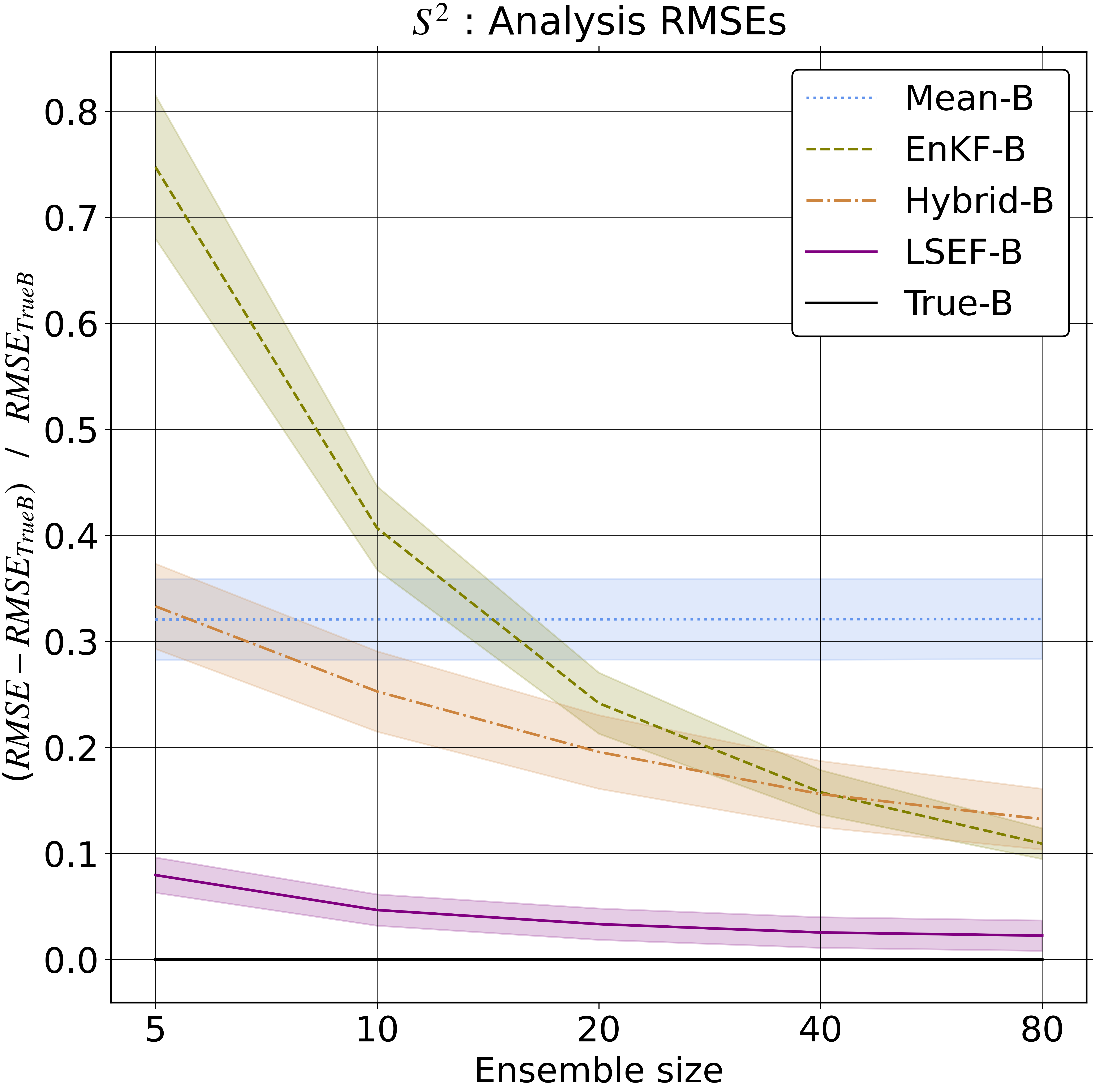
Figure 2: Analysis performance scores (the lower the better, =0 best possible), 90% bootstrap confidence bands (shaded). Dependence on ensemble size.

Figure 3 shows how the five analyses performed with the varying non-stationarity strength parameter $\varkappa$. The LSEF-B analysis’ advantage over EnKF-B was big and nearly uniform for all $\varkappa>1$ on the plot. It was Mean-B that suffered/benefited most from strong/weak non-stationarity, as expected. In the stationary regime (i.e., with $\varkappa=1$), Mean-B was almost as accurate as True-B because ${\bf B}_{\rm mean}$ was estimated by averaging over 33 replicates of the truth (in which the true local spectra were the same, see Appendix H.5) and also by spatial averaging (section 5.1). For this reason, Mean-B could not be rivaled by any ensemble analysis in the stationary regime.

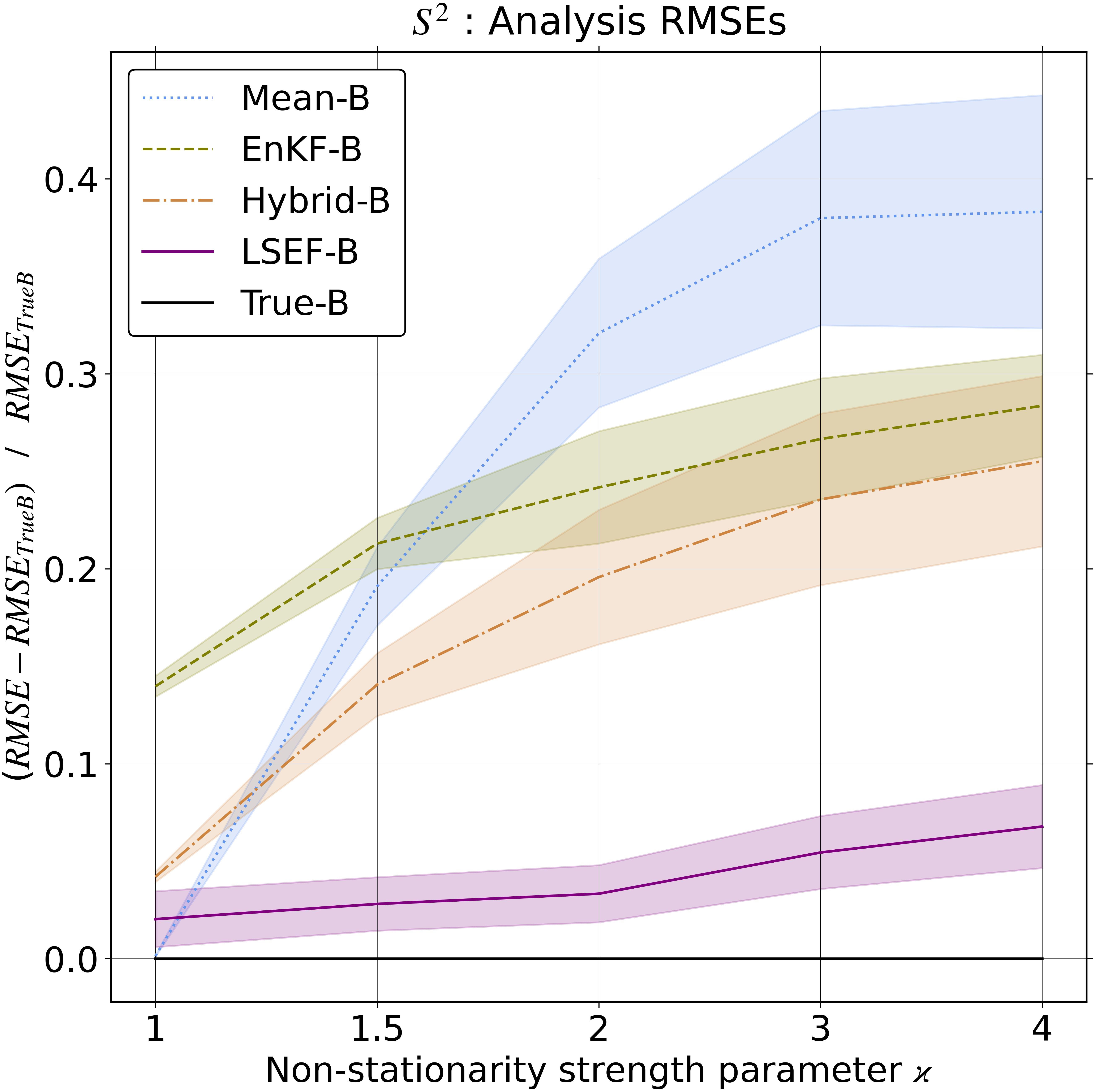
Figure 3: Analysis performance scores (the lower the better, =0 best possible), 90% bootstrap confidence bands (shaded). Dependence on the non-stationarity strength parameter $\varkappa$.

Figure 4 shows how the analyses performed with the varying non-stationarity length parameter $\mu_{\rm NSL}$. Again, LSEF-B was significantly better than the other sub-optimal analyses and that was the case even beyond the local stationarity assumption (section 2.5), which requires that the non-stationarity length scale is much larger than the typical length scale of the field itself. Indeed, LSEF-B was substantially better than the competing techniques even when $\mu_{\rm NSL}=1$ (see Fig.4), that is, when the non-stationarity length scale was equal to the median local length scale (see Eqs. (68) and (65)).

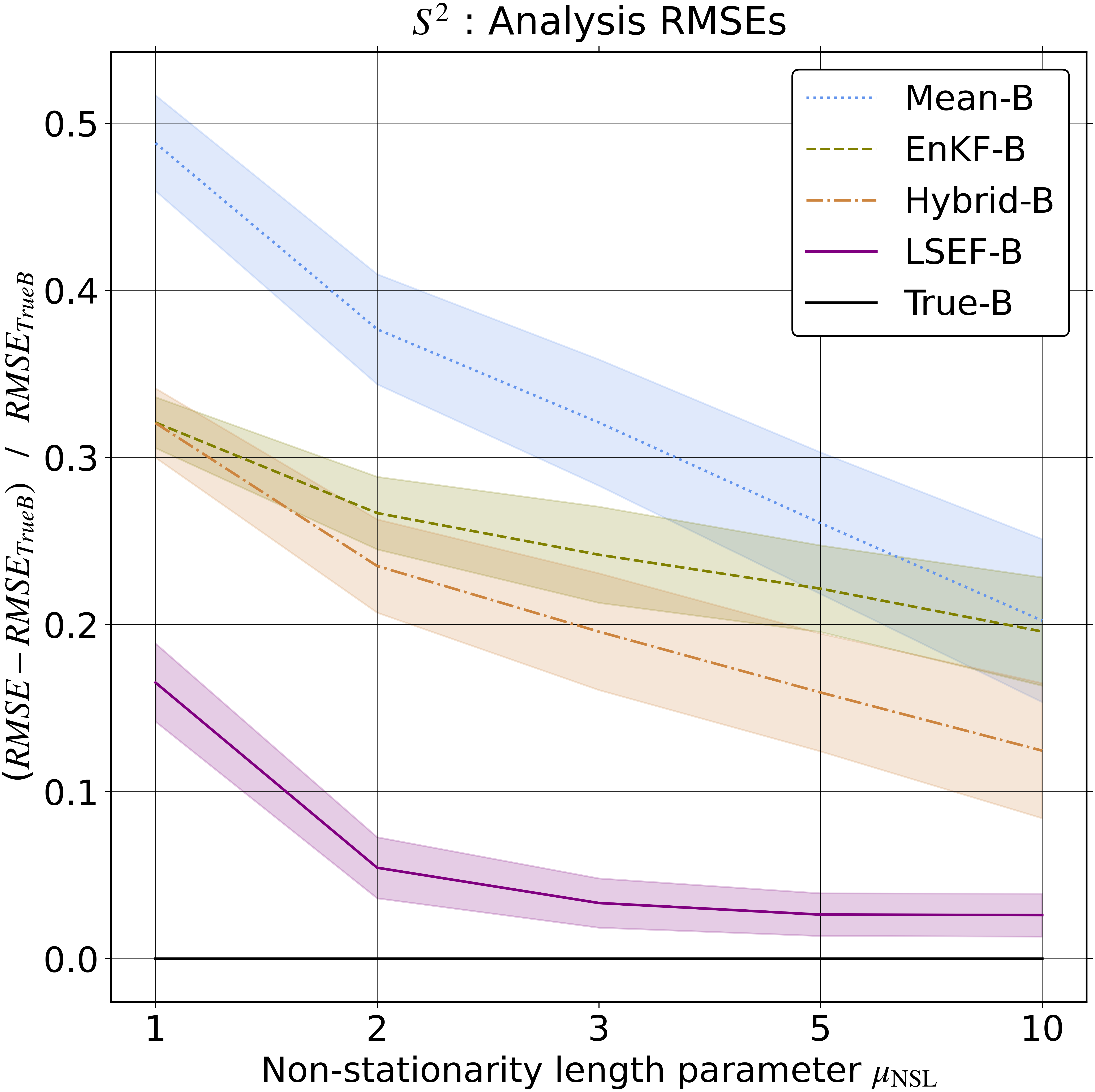
Figure 4: Analysis performance scores (the lower the better, =0 best possible), 90% bootstrap confidence bands (shaded). Dependence on the non-stationarity length parameter $\mu_{\rm NSL}$.

It is important to notice that in LSEF-B, the neural network was trained only once, for the default setup, whereas we had to tune the localization length scale in EnKF-B for each triple $n_{\rm e},\varkappa,\mu_{\rm NSL}$. Similarly, ${\bf B}_{\rm mean}$ was computed for use in Mean-B and Hybrid-B for every pair $\varkappa,\mu_{\rm NSL}$. This suggests that the neural net-based LSEF-B was more robust than the competing analyses.

The neural network was trained on an “archive” of the same volume as we used to calculate ${\bf B}_{\rm mean}$, yet it allowed LSEF-B to exhibit much better results than Hybrid-B. This suggests that the neural network is capable of selective blending of sample covariances with time-mean covariances. This is in contrast to Hybrid-B, which just mixes the two kinds of covariances with, effectively, equal weights for all spatial scales.

We reproduced the above experimental methodology (the model of “truth” and the five analyses) on the circle and obtained qualitatively very similar results (not shown). The code was written by the other author in a different programming language (R vs. Python).

To conclude, when the truth was generated by a (parametric) Locally Stationary Convolution Model, the proposed analysis technique performed very well as compared with the competing techniques. The question remains how the proposed approach will perform in a more realistic situation when background errors do not satisfy a Locally Stationary Convolution Model and true local spectra are not just unavailable but they do not exist? To answer this question we turn to sequential data assimilation.

6 Numerical experiments with LSEF

Here we compare LSEF with the Kalman filter and the three sub-optimal filters whose analyses were tested in section 5. In the sequential filtering experiments reported in this section, the spatial domain was the circle.

6.1 Model of truth and forecast model

To test LSEF we took the Doubly Stochastic Advection-Diffusion-Decay Model [42] :

$${\bf x}_{t}={\bf F}(\boldsymbol{\theta}_{t}){\bf x}_{t-1}+\boldsymbol{\sigma}_{t}\boldsymbol{\varepsilon}_{t},$$ (23)

where ${\bf x}_{t}$ is the spatial field defined on a regular grid on the unit circle (a vector), $t$ is the1 time index, ${\bf F}(\boldsymbol{\theta}_{t})$ is the forecast model operator, $\boldsymbol{\theta}_{t}$ and $\boldsymbol{\sigma}_{t}$ are the spatial “parameter” fields defined below in Eqs. (24) and (25), and $\boldsymbol{\varepsilon}_{t}$ is the standard spatio-temporal white noise. Double stochasticity means that both the forcing $\boldsymbol{\varepsilon}_{t}$ and the parameters $\boldsymbol{\theta}_{t},\boldsymbol{\sigma}_{t}$ are random. The latter are postulated to be stationary (in space and time) random fields satisfying the same model Eq.(23) but with constant non-random coefficients $\theta_{\theta},\theta_{\sigma},\sigma_{\theta},\sigma_{\sigma}$:

$$\boldsymbol{\theta}_{t}={\bf F}(\theta_{\theta})\boldsymbol{\theta}_{t-1}+\sigma_{\theta}\boldsymbol{\varepsilon}_{t}^{\prime},$$ (24)

$$\boldsymbol{\sigma}_{t}={\bf F}(\theta_{\sigma})\boldsymbol{\sigma}_{t-1}+\sigma_{\sigma}\boldsymbol{\varepsilon}_{t}^{\prime\prime},$$ (25)

where $\boldsymbol{\varepsilon}_{t}^{\prime},\boldsymbol{\varepsilon}_{t}^{\prime\prime}$ are independent standard spatio-temporal white noises. Variability in $\boldsymbol{\theta}_{t},\boldsymbol{\sigma}_{t}$ leads to non-stationarity (in space and time) of the conditional distribution ${\bf x}\,|(\boldsymbol{\theta},\boldsymbol{\sigma})$, i.e., when $\boldsymbol{\theta}_{t},\boldsymbol{\sigma}_{t}$ are simulated and fixed in the simulation of ${\bf x}_{t}$.

The reason for using this model was its ability to generate non-stationary random fields ${\bf x}_{t}$ without sacrificing linearity. The linearity of the forecast model allowed us to compare the filters with the unbeatable benchmark, the exact Kalman filter. This is normally not possible with nonlinear forecast models.

In the filters, the forecast model operator was ${\bf F}(\boldsymbol{\theta}_{t})$, and the forcing was zero. First, we generated the parameter fields $\boldsymbol{\theta}_{t},\boldsymbol{\sigma}_{t}$ and computed the model error covariance matrices ${\bf Q}_{t}=\boldsymbol{\sigma}_{t}\boldsymbol{\sigma}_{t}^{\textsf{T}}$ (made available to the Kalman filter only). Then, $\boldsymbol{\theta}_{t},\boldsymbol{\sigma}_{t}$ were fixed and we computed the truth ${\bf x}_{t}$ (as a solution to Eq.(23)) and observations ${\bf x}_{t}^{\rm obs}$ (as the noise-contaminated truth at some grid points and every analysis time instant $t$). After that, having fixed the truth and the observations, we ran the filters.

As a result, we were able to set up and examine the Kalman filter (KF), LSEF, and the three competing ensemble filters: EnKF, the Mean-B filter, and the Hybrid-B filter.

6.2 Filtering setup

The Doubly Stochastic Advection-Diffusion-Decay Model was defined on a 120-point regular grid on the circle (so that $\ell_{\rm max}=60$). Otherwise, its setup coincided with that reported in [42].

The ensemble size was between 5 and 80 with the default 10. The number of bandpass filters and the setup of the neural network were the same as in the above experiments on the sphere. 5000 consecutive assimilation cycles were used to validate the filters. ${\bf B}_{\rm mean}$ was computed by averaging the Kalman filter’s ${\bf B}$ over 50,000 cycles and, additionally, by averaging in space. The latter was done by averaging entries of ${\bf B}$ over its main diagonal (getting the mean variance) and each cyclic super-diagonal (getting the whole set of mean covariances). “Synthetic” observations were located at every 10th model grid point. The observation error variance was specified to roughly match the mean Kalman-filter forecast error variance.

In EnKF and Hybrid-B filter, multiplicative covariance inflation (e.g., Houtekamer and Zhang [19])) was used. Ensemble perturbations were multiplied by a factor slightly greater than one tuned to optimize the filter performance. The multiplier 1.02 was used in all experiments. There was no covariance inflation in LSEF (as we found that it deteriorated its performance, not shown).

6.3 Training sample

In LSEF, the forecast error field does not obey the Locally Stationary Convolution Model, its imposition in the LSEF analysis is an approximation. Therefore, in the course of filtering, we had no access to true local spectra (as they do not exist in this setting) and thus could not immediately apply the technique described in section 5.3 to train the neural network, which, we recall, recovers the local spectrum from the set of sample band variances (section 3.3) for each grid point separately.

To build the training sample, we initially tried to manually set up the Parametric Locally Stationary Convolution Model (described in Appendix H) so that the spatial non-stationarity of variances and local length scales in the generated pseudo-random fields resembled those of the forecast-error fields we obtained in the course of Kalman filtering. In that way, we were able to generate the training sample following section 5.3. But the filtering results were mediocre (not shown). Another option we tested was to fit, having the EnKF forecast ensemble at every assimilation cycle, the Locally Stationary Convolution Model. The fitted model provided us with the estimated local spectra, which were then used in the training sample. The respective sample band variances were computed from a new ensemble generated by the fitted model. This approach did yield an improvement, but the following technique was somewhat more successful (and it was also better than the linear pseudo-inversion-based technique outlined in section 3.3) and so was used in the experiments presented below.

During an EnKF run, at each assimilation cycle $t=1,\dots,50,000$, we performed spatial averaging of the forecast-ensemble sample covariance matrices ${\bf S}_{t}$ (see how ${\bf B}_{\rm mean}$ was computed in section 6.2). The resulting spatially averaged covariance functions $b_{t}(x)$ with $x=0,\dots,n_{\rm x}/2$ were stored. Then, offline, for each covariance function $b_{t}(x)$ we computed its spectrum (Fourier transform) $f_{t}(\ell)$. Knowing $f_{t}(\ell)$, we computed, for each $t$, an ensemble of pseudo-random realizations of the respective (stationary) random process, subjected them to the spatial bandpass filters (section 3.1), and finally computed the vectors $\widehat{\bf v}_{t}$ of sample band variances (section 3.2). The resulting training sample consisted of 50,000 pairs $(\widehat{\bf v}_{t},f_{t}(.))$. The above spatial averaging of EnKF sample covariances reduced the diversity in the training sample. To compensate for that effect, we set up the Doubly Stochastic Advection-Diffusion-Decay Model in the strongly non-stationary regime [42, Table 3] when running EnKF to generate the training sample.

6.4 Results

The performance of each of the five filters was measured by the RMSE (with respect to the truth) of their control forecasts ${\bf x}^{\rm f}_{t}$. The RMSE was computed by averaging over the spatial grid, over 5000 assimilation cycles, and over 10 replicates of the parameter fields $\boldsymbol{\theta}_{t},\boldsymbol{\sigma}_{t}$ of the model of truth. As in section 5.4, we show here the analysis performance score Eq.(22), where ${\rm RMSE}_{\rm TrueB}$ is the RMSE of Kalman filter’s forecasts.

We compared the five filters with different ensemble sizes and in four regimes of non-stationarity of the true spatio-temporal field. The regimes are labeled by numbers from 0 (stationarity) to 3 (strong non-stationarity). For a more detailed description of the non-stationarity regimes, see Tsyrulnikov and Rakitko [42]. The default non-stationarity regime was 2.

Figure 5 shows that LSEF was better than the competing EnKF, Mean-B, and Hybrid-B filters for small to medium ensemble sizes. With large $n_{\rm e}$, LSEF was comparable to or somewhat worse than the competing filters. Comparing Fig.5 with Fig.2 demonstrates that the great advantage of LSEF observed when the truth was generated by the Parametric Locally Stationary Convolution Model (Fig.2) was more modest in a more realistic situation here (Fig.5). Nevertheless, the superiority of LSEF for $n_{\rm e}\leq 20$ was substantial. Note also that the ensemble size of 80 is much larger as compared with the spatial grid size (120) than it normally is for high-dimensional systems.

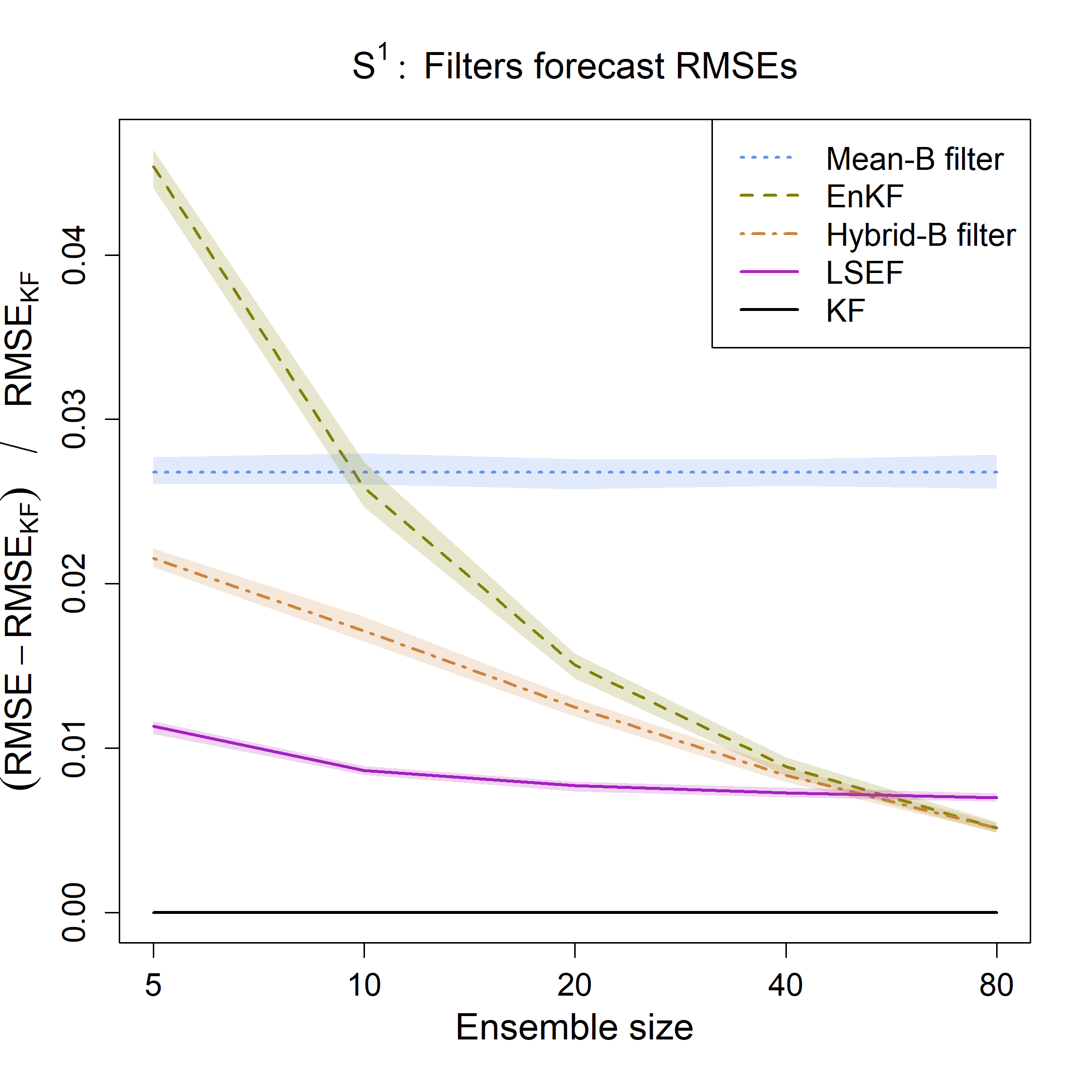
Figure 5: Filters performance scores (the lower the better, =0 best possible), 90% bootstrap confidence bands (shaded). Dependence on ensemble size.

Figure 6 shows how the five filters performed under different non-stationarity regimes. The superiority of LSEF was nearly uniform except for the stationary regime 0. Like in section 5.4 (see Fig.4 at $\mu_{\rm NSL}=1$), the advantage of LSEF remained substantial even under strong non-stationarity (regime 3 on the x-axis in Fig.6).

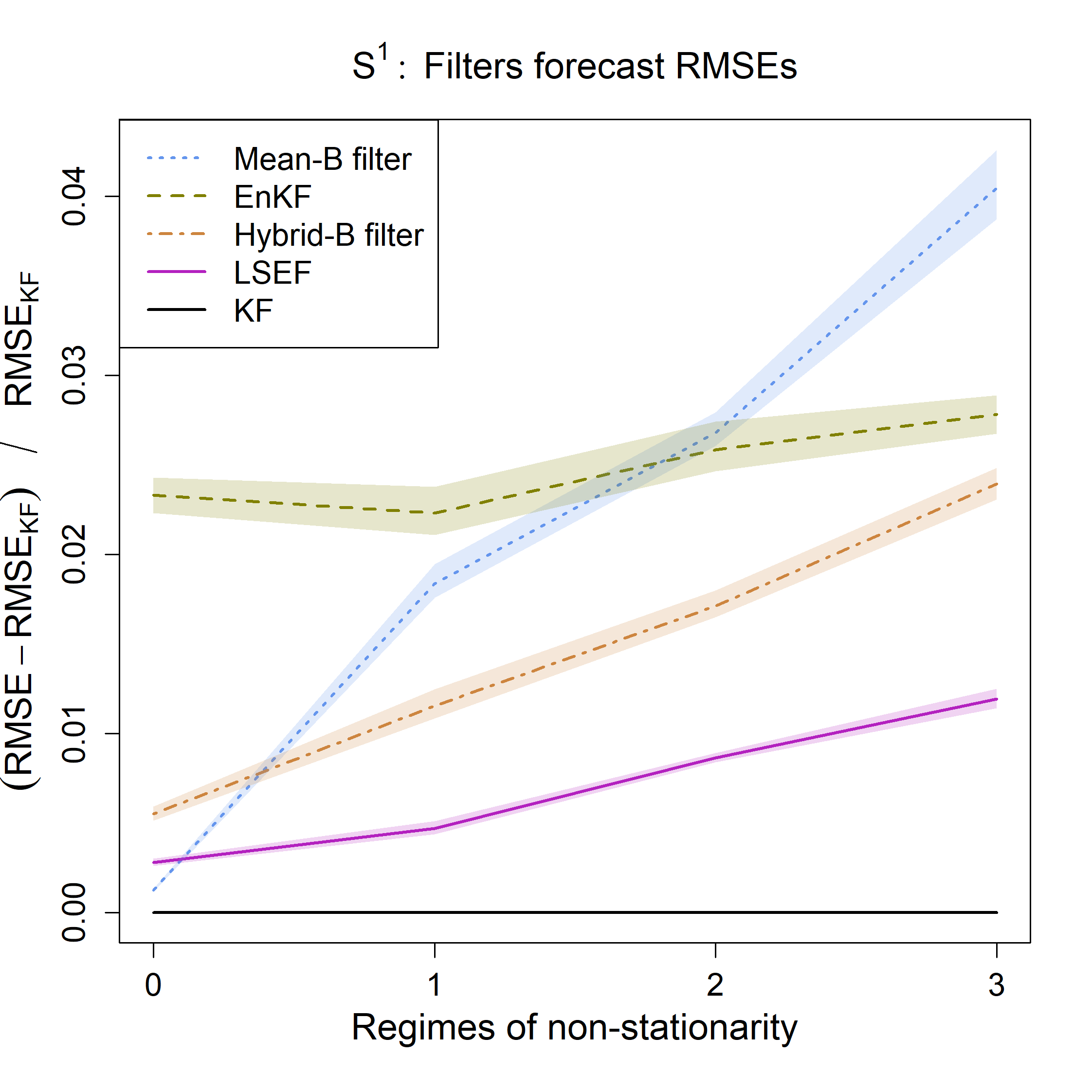
Figure 6: Filters performance scores (the lower the better, =0 best possible), 90% bootstrap confidence bands (shaded). Dependence on the non-stationarity regime.

7 Discussion and conclusions

In this research, we have proposed the Locally Stationary Convolution Model and used it to regularize the observation-update (analysis) step of an ensemble-based sequential filter. The spatial model is formulated (on the sphere and the circle) for the underlying forecast error random field rather than for its spatial covariances, which guarantees that the model is well-posed. The model is non-stationary, which can be essential for real-world (e.g., geoscientific) applications, and non-parametric, which allows for more diverse shapes of spatial covariances as compared to parametric models. Local stationarity means that the process can be approximated by a stationary process locally in space. The non-trivial local stationarity takes place whenever the typical length scale of the process is much less than the non-stationarity length scale, the scale on which the local structure of the process varies in space. The stationary process convolution model is a special case of our non-stationary model (note that this is in contrast to the wavelet-diagonal model).

Local stationarity allowed us to build a model estimator using spatial bandpass filters. The sample variance of the output of a bandpass filter (sample band variance) at some grid point $x$ is a weighted average of the raw sample (ensemble) covariances in a vicinity of $x$. This averaging reduces sampling noise but may lead to excessive smoothing of the spatial covariances. If the averaging length scale, which equals the width of the spatial filter’s impulse response function, is significantly smaller than the non-stationarity length scale, then such averaging does not lead to a significant systematic distortion of the spatial covariances. The main hypothesis underlying this research is that there are filtering problems in which the reduction in sampling noise (i.e., in the random uncertainty) has a greater positive impact on the filter’s accuracy than the negative effect of the induced systematic uncertainty in the filter’s prior distribution. Our numerical experiments suggest that this hypothesis is plausible.

We postulated that in the course of sequential ensemble filtering, the forecast error field obeys the Locally Stationary Convolution Model. As a result, we obtained a new sequential filter termed the Locally Stationary convolutional Ensemble Filter (LSEF). Testing the filter with a non-stationary spatio-temporal model of truth yielded encouraging results. It is worth noting that ad-hoc regularization devices like localization and covariance inflation, which are, normally, used (and employed in our experiments) in EnKF and hybrid filters were absent in LSEF. This can be important in practice since ad-hoc devices require extensive (and expensive) tuning. Another interesting result is that the advantage of LSEF was observed not only under weak non-stationarity, as intended, but in strongly non-stationary regimes as well.

The tests of our spatial-model-based covariance regularization technique were conducted with linear observation models on the sphere and linear forecast and observation models on the circle. We believe that linearity of these tests is not a significant restriction, expecting that the technique will be useful whenever an EnKF-like filter is useful, that is, with non-linear models as well.

Using a neural network to recover local spectra from the ensemble proved to be successful. The network was capable of more efficient extraction of information from the ensemble as compared to the more conventional approaches we tried. Even in the situation when true (target) local spectra were not available to train the net (in sequential filtering), it did yield the best results. In case when the target local spectra were available (in our experiments with static analyses on the sphere) and they were used to build the training sample, the advantage of the neural network was dramatic. Our results also suggest that the neural net was more successful in extracting “climatological” information from the training sample and combining it with the information provided by the forecast ensemble than the widely-used linear combination of static and localized ensemble covariance matrices.

Applying the developed sequential filtering technique to real-world high-dimensional problems will require a computationally efficient multi-grid/multi-scale version of the algorithm. Work on it is underway. Its non-ensemble version (with static spatial covariances) has been successfully tested in an operational meteorological data assimilation system [43]. Adding the ensemble component should be affordable as well because the spatial model estimator consists of computationally cheap spatial filters followed by a grid point-by-grid point application of a small neural network. A three-dimensional extension of the methodology proposed and tested in this research is expected to be straightforward. Further extensions to the spatial model may include directional anisotropy and, possibly, non-Gaussianity.

Acknowledgements

We would like to thank Dmitry Gayfulin, who conducted preliminary numerical experiments at an early stage of this study. The study has been conducted under Task 1.1.1 of scientific research and technology Plan of the Russian Federal Service for Hydrometeorology and Environmental Monitoring.

Appendices

Appendix A Spherical harmonics and Legendre polynomials

The normalization of spherical harmonics is such that they are orthonormal w.r.t. the inner product $(\psi_{1},\psi_{2})=\int_{{\mathbb{S}}^{2}}\psi_{1}(x)\psi_{2}^{*}(x)\,{\rm d}x$, where the asterisk denotes complex conjugation and $x$ stands for a point on the unit sphere.

The normalization of Legendre polynomials is such that $P_{\ell}(1)=1$.

The addition theorem for spherical harmonics reads

$$\sum_{m=-\ell}^{\ell}Y_{\ell m}(x)Y_{\ell m}^{*}(y)=\frac{2\ell+1}{4\pi}P_{\ell}(\cos\rho(x,y)),$$ (26)

where $x$ and $y$ are two points on the unit sphere and $\rho(x,y)$ is the great-circle distance between them.

By the forward Fourier-Legendre transform of a function, $F(\rho)$ (where $\rho\in[0,\pi]$), we mean the set of real numbers $\widetilde{F}_{\ell}$ (where $\ell=0,1,\dots,\ell_{\rm max}$) defined by the formula

$$\widetilde{F}_{\ell}=2\pi\int_{0}^{\pi}F(\rho)P_{\ell}(\cos\rho)\sin\rho\,{\rm d}\rho.$$ (27)

The backward Fourier-Legendre transform is then

$$F(\rho)=\sum^{\ell_{\rm max}}_{\ell=0}\frac{2\ell+1}{4\pi}\,\widetilde{F}_{\ell}\,P_{\ell}(\cos\rho).$$ (28)

Appendix B Locally Stationary Convolution Model on the unit circle

On ${\mathbb{S}}^{1}$, the model Eq.(6) specializes to

$$\xi(x)=\int_{{\mathbb{S}}^{1}}u(x,y-x)\,\alpha(y)\,{\rm d}y,$$ (29)

where the real-valued convolution kernel $u(x,z)$ is an even function of the second argument. Let us employ the truncated Fourier series expansion of the kernel in the form

$$u(x,z)=\frac{1}{\sqrt{2\pi}}\sum_{\ell=-\ell_{\rm max}}^{\ell_{\rm max}}\sigma_{\ell}(x)\,\mathrm{e}^{\mathsf{i}\ell z}.$$ (30)

Here $\sigma_{\ell}(x)$ are real-valued functions such that $\sigma_{-\ell}(x)=\sigma_{\ell}(x)$. With the positive-definite kernel assumption (section 2.4), $\sigma_{\ell}(x)>0$.

In the spectral expansion of the band-limited Gaussian white noise,

$$\alpha(y)=\frac{1}{\sqrt{2\pi}}\sum_{\ell=-\ell_{\rm max}}^{\ell_{\rm max}}\widetilde{\alpha}_{\ell}\,\mathrm{e}^{\mathsf{i}\ell y},$$ (31)

$\widetilde{\alpha}_{\ell}$ are mutually uncorrelated zero-mean and unit-variance random variables. $\widetilde{\alpha}_{0}$ is real valued and the others are complex valued circularly symmetric random variables.

Substituting Eqs. (30) and (31) into Eq.(29) yields the Locally Stationary Convolution Model on the circle:

$$\xi(x)=\sum_{\ell=-\ell_{\rm max}}^{\ell_{\rm max}}\sigma_{\ell}(x)\,\widetilde{\alpha}_{l}\,\mathrm{e}^{\mathsf{i}\ell x},$$ (32)

for which the local spectrum is defined as $f_{\ell}(x)=\sigma_{\ell}^{2}(x)$. From Eq.(32) it follows that the Locally Stationary Convolution Model’s covariances on ${\mathbb{S}}^{1}$ are

$$B(x,x+z)=\operatorname{\mathbb{E}}\xi(x)\xi(x^{\prime})=\sum\,\sigma_{\ell}(x)\,\sigma_{\ell}(x+z)\,\mathrm{e}^{\mathsf{i}\ell z}.$$ (33)

Appendix C Identifiability of the model

Here we consider the process convolution model with the isotropic real-valued kernel $u(x,\rho)$ that is a positive definite function of $\rho$ for any $x$. We prove that if the non-stationary covariances $B(x,x^{\prime})$ are produced by this model, then the model is unique, i.e., the spectral functions $\sigma_{\ell}(x)$ are uniquely determined by $B(x,x^{\prime})$. For simplicity, we consider the circular case.

Let us start with expanding $\sigma_{\ell}(x)$ into the truncated Fourier series

$$\sigma_{\ell}(x)=\sum_{q=-Q}^{Q}\,\widetilde{\sigma}_{\ell q}\,\mathrm{e}^{\mathsf{i}qx},$$ (34)

where $Q$ is the half-bandwidth of the processes $\sigma_{\ell}(x)$ as functions of location $x$. Note that since $\sigma_{-\ell}(x)=\sigma_{\ell}(x)$ (see appendix B), we have $\widetilde{\sigma}_{-\ell,q}=\widetilde{\sigma}_{\ell q}$. Since $\sigma_{\ell}(x)$ is real valued, we have $\widetilde{\sigma}_{\ell,-q}=\widetilde{\sigma}_{\ell q}^{*}$.

We assume that the bandwidth $[-Q,Q]$ is tight in the sense that $\widetilde{\sigma}_{\ell Q}\neq 0$ for all $\ell$.

Let us substitute the expansion Eq.(34) into Eq.(32) and change the summation variable $q$ to $n=\ell+q$:

$$\xi(x)=\sum_{\ell=-L}^{L}\widetilde{\alpha}_{\ell}\,\mathrm{e}^{\mathsf{i}\ell x}\sum_{q=-Q}^{Q}\,\widetilde{\sigma}_{\ell q}\,\mathrm{e}^{\mathsf{i}qx}=\sum_{n=-N}^{N}\widetilde{\xi}_{n}\,\mathrm{e}^{\mathsf{i}nx},$$ (35)

where $N=L+Q$ and

$$\widetilde{\xi}_{n}=\sum_{\begin{subarray}{c}\ell=n-Q\\ |\ell|\leq L\end{subarray}}^{n+Q}\widetilde{\alpha}_{\ell}\,\widetilde{\sigma}_{\ell,n-\ell},$$ (36)

Since the bandwidth for $\xi(x)$ is finite, $\xi(x)$ is uniquely represented by the set of its spectral coefficients $\{\widetilde{\xi}_{n}\}_{n=-N}^{N}$. Therefore the covariances $B(x,x^{\prime})$ are uniquely represented by the set of the spectral covariances $\widetilde{\bf B}_{n\bar{n}}=\operatorname{\mathbb{E}}\widetilde{\xi}_{n}\widetilde{\xi}_{\bar{n}}^{*}$. Now, we derive $\widetilde{\bf B}_{n\bar{n}}$ from Eq.(36) taking into account that $\widetilde{\alpha}_{\ell}$ are all mutually uncorrelated zero-mean unity-variance random variables:

$$\widetilde{\bf B}_{n\bar{n}}=\operatorname{\mathbb{E}}\sum_{\begin{subarray}{c}\ell=n-Q\\ |\ell|\leq L\end{subarray}}^{n+Q}\widetilde{\alpha}_{\ell}\,\widetilde{\sigma}_{\ell,n-\ell}\sum_{\begin{subarray}{c}\bar{\ell}=\bar{n}-Q\\ |\bar{\ell}|\leq L\end{subarray}}^{\bar{n}+Q}\widetilde{\alpha}_{\bar{\ell}}^{*}\,\widetilde{\sigma}_{\bar{\ell},\bar{n}-\bar{\ell}}^{*}=\sum_{\begin{subarray}{c}\ell=n-Q\\ |\ell|\leq L\end{subarray}}^{n+Q}\widetilde{\sigma}_{\ell,n-\ell}\,\widetilde{\sigma}_{\ell,\bar{n}-\ell}^{*}$$ (37)

and show that all $\widetilde{\sigma}_{\ell q}$ are uniquely determined by Eq.(37). The summation area in Eq.(37) for all possible $n$ and $\bar{n}$ is shown in Fig.7 for $L=2$ and $Q=1$.

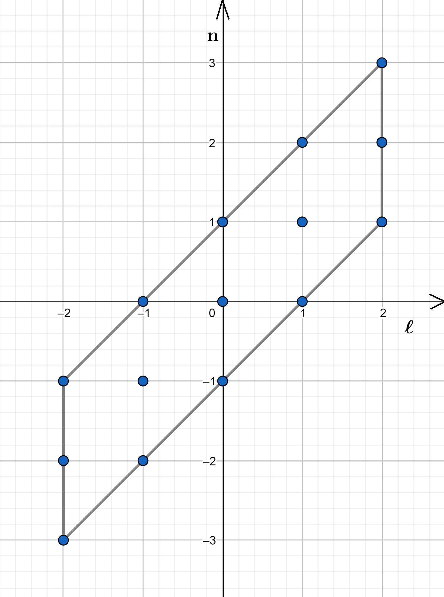
Figure 7: Circular case. Summation area for $L=2$ and $Q=1$

We start with $n=N\equiv L+Q$, for which the sum in Eq.(36) reduces to the single term, $\widetilde{\xi}_{N}=\widetilde{\alpha}_{L}\,\widetilde{\sigma}_{LQ}$ (the upper right corner of the summation area in Fig.7). This means that the covariance of $\widetilde{\bf B}_{Nn}=\operatorname{\mathbb{E}}\widetilde{\xi}_{N}\,\widetilde{\xi}_{n}^{*}$ for any $n\in[L-Q,L+Q]$ will also contain just one term, $\widetilde{\bf B}_{Nn}=\widetilde{\sigma}_{LQ}\,\widetilde{\sigma}^{*}_{L,n-L}$ so that we can uniquely restore $\widetilde{\sigma}_{Lq}$ for all $q$. To realize this, we note, first, that $\widetilde{\bf B}_{NN}=|\widetilde{\sigma}_{LQ}|^{2}$. Next, we turn to $\widetilde{\bf B}_{N,L-Q}=\widetilde{\sigma}_{LQ}\,\widetilde{\sigma}_{L,-Q}^{*}$ (the lower right corner of the summation area in Fig.7). Recalling that $\widetilde{\sigma}_{\ell,-q}=\widetilde{\sigma}_{\ell q}^{*}$, we obtain $\widetilde{\bf B}_{N,L-Q}=\widetilde{\sigma}_{LQ}^{2}$. So, from $\widetilde{\bf B}_{NN}\equiv\widetilde{\bf B}_{N,L+Q}$ and $\widetilde{\bf B}_{N,L-Q}$ we know both the modulus and the square of the complex number $\widetilde{\sigma}_{LQ}$, hence it is uniquely determined, up to the sign. By the tight bandwidth assumption, $\widetilde{\sigma}_{LQ}\neq 0$, therefore, we recover $\widetilde{\sigma}_{Lq}$ for all $|q|<Q$ from $\widetilde{\bf B}_{N,L+q}=\widetilde{\sigma}_{LQ}\,\widetilde{\sigma}_{Lq}^{*}$ (the right edge of the summation parallelogram in Fig.7), again, up to the sign. The ambiguity in the sign disappears when it comes to $\widetilde{\sigma}_{L0}$, which is positive because $\sigma_{\ell}(x)>0$ due to the positive-definiteness constraint (item 2 in section 2.7 and Appendix B). Thus, $\widetilde{\sigma}_{Lq}$ are uniquely recovered for all $q$ from the model covariances.

Then, we consider $\widetilde{\xi}_{N-1}$ and realize that it, again, has just one term, $\widetilde{\alpha}_{L-1}\,\widetilde{\sigma}_{L-1,L-1+Q}$ besides the term that contains $\widetilde{\sigma}_{L,L+Q-1}$, which has already been recovered. This allows us to repeat the above process and recover $\widetilde{\sigma}_{L-1,L-1+q}$ for all $q\in[-Q,Q]$. And so on, we uniquely recover all non-zero $\widetilde{\sigma}_{\ell q}$, and therefore all spectral functions $\sigma_{\ell}(x)$, from the set of spectral covariances $\widetilde{\bf B}_{n\bar{n}}$. This completes the proof that the Locally Stationary Convolution Model on the circle is unique provided that the convolution kernel $u(x,z)$ is real valued, is an even function of $z$, and the half-bandwidth $Q$ of $\sigma_{\ell}(x)$ is such that $\widetilde{\sigma}_{\ell Q}\neq 0$ for any $\ell$. On ${\mathbb{S}}^{2}$, the same reasoning is applicable (not shown).

Appendix D The most localized kernel in the stationary case

Here we show that an isotropic convolution kernel whose convolution with the white noise is a stationary process with the given spatial spectrum (equivalently, with the given covariance function) is not unique. Uniqueness can be achieved by requiring that the kernel be most spatially localized.

Consider a stationary (isotropic) process on the sphere defined by its spectral representation

$$\xi_{\rm statio}(x)=\sum^{\ell_{\rm max}}_{\ell=0}\sum^{\ell}_{m=-\ell}\,\widetilde{\xi}_{\ell m}\,Y_{\ell m}(x)\equiv\sum^{\ell_{\rm max}}_{\ell=0}\sum^{\ell}_{m=-\ell}\,\sigma_{\ell}\,\widetilde{\alpha}_{\ell m}\,Y_{\ell m}(x),$$ (38)

where it is straightforward to see that $\operatorname{\mathbb{E}}\widetilde{\xi}_{\ell m}\widetilde{\xi}_{\ell^{\prime}m^{\prime}}^{*}=\sigma_{\ell}^{2}\,\delta_{\ell}^{\ell^{\prime}}\delta_{m}^{m^{\prime}}.$ The process $\xi_{\rm statio}(x)$ can be modeled as the convolution of the kernel

$$u(\rho)=\sum\frac{2\ell+1}{4\pi}\sigma_{\ell}P_{\ell}(\cos\rho)$$ (39)

with the white noise $\alpha$ (see Eq.(9)):

$$\xi_{\rm statio}(x)=\int u(\rho(x,y))\,\alpha(y)\,{\rm d}y.$$ (40)

Multiple kernels $u(\rho)$ give rise to the same spectrum $f_{\ell}=\sigma_{\ell}^{2}$ of the process $\xi_{\rm statio}(x)$, differing one from another in the signs of $\sigma_{\ell}$ (recall that with the real-valued kernel $u(\rho)$, all $\sigma_{\ell}$ are real valued). To isolate a unique kernel, we require it to be most spatially localized in the sense that it has a minimal width. We define the width as a kind of macro-scale from

$$R^{2}_{\rm u}=\frac{\int_{{\mathbb{S}}^{2}}u^{2}(\rho(x,y))\,{\rm d}y}{(\max|u(\rho)|)^{2}}.$$ (41)

Here, the numerator is equal to $\sum\frac{2\ell+1}{4\pi}f_{\ell}$ and thus is fixed given the spectrum $f_{\ell}$. So, $R_{\rm u}$ is minimized when $\max|u(\rho)|$ is maximal among all kernels with the fixed $|\sigma_{\ell}|$. That is, we seek to maximize $|u(\rho)|$ over both $\rho$ and the signs of $\sigma_{\ell}$. From Eq.(39), we have

$$|u(\rho)|=\left|\sum^{\ell_{\rm max}}_{\ell=0}\frac{2\ell+1}{4\pi}\sigma_{\ell}P_{\ell}(\cos\rho)\right|\leq\sum^{\ell_{\rm max}}_{\ell=0}\frac{2\ell+1}{4\pi}|\sigma_{\ell}|$$ (42)

because $|P_{\ell}(t)|\leq 1$ for $-1\leq t\leq 1$ [38, section 7.21]. Since $|P_{\ell}(t)|=1$ if and only if $t=\pm 1$, the upper bound (i.e., the maximum of $|u(\rho)|$) indicated in Eq.(42) is reached if all $|P_{\ell}(\cos\rho)|=1$ (which implies that $\rho=0$ or $\rho=\pi$) and all products $\sigma_{\ell}P_{\ell}(\cos\rho)$ have the same sign. This happens in three cases so that there are three solutions to the optimization problem $R_{\rm u}\to\min$.

The first solution is $\sigma_{\ell}>0$ for all $\ell$. The corresponding kernel $u_{1}(\rho)$ is positive definite and its modulus is maximized at $\rho=0$.

The second solution is $\sigma_{\ell}\leq 0$ for all $\ell$. The corresponding kernel $u_{2}(\rho)$ is non-positive definite and its modulus is maximized at $\rho=0$ so that $u_{2}(\rho)=-u_{1}(\rho)$.

The third solution is $\sigma_{\ell}=(-1)^{\ell}|\sigma_{\ell}|$. The corresponding kernel $u_{3}(\rho)$ is non-definite, its modulus is maximized at $\rho=\pi$, and $u_{3}(\rho)=u_{1}(\pi-\rho)$ (this follows from the identity $P_{\ell}(-t)=(-1)^{\ell}P_{\ell}(t)$).

As the above three kernels that minimize the length scale $R_{\rm u}$ have the same shape, we select the first solution: the positive definite kernel $u(\rho)$.

On the circle, similar arguments lead to virtually the same conclusion: the most localized kernel is a positive definite function $u(x)$ or its negated/translated version $\pm u(x-h)$ (for any $h\in{\mathbb{S}}^{1}$, the proof is omitted).

Appendix E Local stationarity

The notion of local stationarity has been defined differently by different authors (most often for processes on the real line). The general idea is that a locally stationary process can be approximated by a stationary process locally, i.e., in a vicinity of any point in time [29]. Starting from Dahlhaus [8], the common approach is to use the “infill” asymptotics, which considers the process $\xi(t)$ in rescaled time $t/T$ with $t=0,1,\dots,T$ and $T\to\infty$. With this approach, effectively, just one segment of the non-stationary process is studied in increasingly sharper detail.

On compact manifolds like the circle or the sphere, this rescaling cannot be used because of their compactness. Here we outline a different approach to local stationarity with our spatial model. For simplicity, we consider the circular case (extensions to the spherical case are straightforward).

Recall that the non-stationary random process in question is defined as $\xi(x)=\sum\sigma_{\ell}(x)\,\widetilde{\alpha}_{l}\,\mathrm{e}^{\mathsf{i}\ell x}$ (Eq.(32)). As its non-stationarity comes from the dependencies of $\sigma_{\ell}$ on the location $x$, let us assume that these are caused by $\sigma_{\ell}(x)$ being random processes themselves. More specifically, we postulate that $\sigma_{\ell}(x)$ are, jointly, a vector-valued mean-square differentiable stationary random process. Then, we obtain spatial non-stationarity by considering the conditional distribution of $\xi(.)$ given all $\sigma_{\ell}(.)$. We denote this conditioning by $\xi\,|\,\sigma$.

Now, we can define the length scale $\Lambda_{\ell}$ of the stationary process $\sigma_{\ell}(x)$ as the micro-scale from the equation

$$\operatorname{\mathbb{E}}\left(\frac{\partial\sigma_{\ell}}{\partial x}\right)^{2}=\frac{{\mathsf{Var}}\,\sigma_{\ell}}{\Lambda_{\ell}^{2}}.$$ (43)

If $\min_{\ell}(\Lambda_{\ell})=\Lambda>0$, we call $\Lambda$ the non-stationarity length scale.

Next, we define the characteristic length scale $L$ of the process $\xi(x)$ from

$$L^{2}=\frac{\sum\operatorname{\mathbb{E}}\sigma_{\ell}^{2}}{\sum\ell^{2}\operatorname{\mathbb{E}}\sigma_{\ell}^{2}},$$ (44)

i.e., as the inverse width of the mean local spectrum.

Finally, we define the non-stationarity strength per wavenumber,

$$S_{\ell}=\frac{{\mathsf{Var}}\,\sigma_{\ell}}{\operatorname{\mathbb{E}}^{2}\sigma_{\ell}},$$ (45)

which quantifies the magnitude of the random component in the local spectrum. Let the overall non-stationarity strength be $S=\max_{\ell}S_{\ell}\in[0,1)$.

Having defined $\Lambda$, $L$, an $S$, we find conditions under which $\xi(x)$ is locally stationary in the sense that, for any point $x_{0}$, there is an approximating stationary random process $\zeta(x;x_{0})$ such that $\operatorname{\mathbb{E}}\operatorname{\mathbb{E}}[(\xi(x)-\zeta(x;x_{0}))^{2}\,|\,\sigma]\ll\operatorname{\mathbb{E}}\operatorname{\mathbb{E}}[\xi^{2}(x)\,|\,\sigma]$ whenever $|x-x_{0}|\leq L$. Formally, we can consider the limit $\Lambda\to\infty$, that is, the large $\Lambda$ asymptotics, but we prefer to specify in which sense $\Lambda$ can be considered “large” in a practical situation.

We define the approximating process as $\zeta(x;x_{0})=\sum\sigma_{\ell}(x_{0})\,\widetilde{\alpha}_{l}\,\mathrm{e}^{\mathsf{i}\ell x}$. Then, the mean approximation error variance is

$$\operatorname{\mathbb{E}}\operatorname{\mathbb{E}}[(\xi(x)-\zeta(x;x_{0}))^{2}\,|\,\sigma]=\sum\operatorname{\mathbb{E}}(\sigma_{\ell}(x)-\sigma_{\ell}(x_{0}))^{2}=\\ \sum\operatorname{\mathbb{E}}\left(\frac{\partial\sigma_{\ell}}{\partial x}\right)^{2}(x-x_{0})^{2}\leq\left(\frac{L}{\Lambda}\right)^{2}\sum{\mathsf{Var}}\,\sigma_{\ell}.$$ (46)

Here, the derivatives are taken at points between $x_{0}$ and $x$. The inequality is due to Eq.(43), $\Lambda\leq\Lambda_{\ell}$, and $|x-x_{0}|\leq L$. Noting that $\operatorname{\mathbb{E}}\operatorname{\mathbb{E}}[\xi^{2}(x)\,|\,\sigma]=\sum\operatorname{\mathbb{E}}\sigma_{\ell}^{2}=\sum(\operatorname{\mathbb{E}}^{2}\sigma_{\ell}+{\mathsf{Var}}\,\sigma_{\ell})$, we write down the relative approximation error variance:

$$\frac{\operatorname{\mathbb{E}}\operatorname{\mathbb{E}}[(\xi(x)-\zeta(x;x_{0}))^{2}\,|\,\sigma]}{\operatorname{\mathbb{E}}\operatorname{\mathbb{E}}[\xi^{2}(x)\,|\,\sigma]}\leq\frac{\sum{\mathsf{Var}}\,\sigma_{\ell}}{\sum\operatorname{\mathbb{E}}^{2}\sigma_{\ell}+\sum{\mathsf{Var}}\,\sigma_{\ell}}\left(\frac{L}{\Lambda}\right)^{2}\leq S\left(\frac{L}{\Lambda}\right)^{2}.$$ (47)

This equation reveals that the locally stationary approximation is precise whenever $S\ll 1$ (and $\Lambda\geq L$) or $\Lambda\gg L$. The case of low non-stationarity strength, $S\ll 1$, is rather trivial because then the process is almost stationary. The non-trivial local stationarity occurs when the non-stationarity length scale is large enough, $\Lambda\gg L$, whatever the non-stationarity strength $S$.

If $\Lambda\gg L$, then it is easy to see that $L_{\xi}\approx L$, where $L_{\xi}$ is defined through $\operatorname{\mathbb{E}}\operatorname{\mathbb{E}}(\xi_{x}^{2}\,|\,\sigma)={\operatorname{\mathbb{E}}\operatorname{\mathbb{E}}(\xi^{2}\,|\,\sigma)}/{L_{\xi}^{2}}$ and $L$ is defined in Eq.(44). For this reason, we call $L$ the characteristic length scale of the process in question $\xi(x)$.

Appendix F Accuracy of the estimator of band variances

Here we consider spatial bandpass filtering of a random process governed by the Locally Stationary Convolution Model and assess errors of the approximations given in Eqs. (13) and (14). For simplicity of presentation, we examine the circular case.

Let the bandpass filter ${\cal H}$ have the spectral transfer function

$$H(\ell)=\kappa\left(\frac{\ell-\ell^{\rm c}}{d}\right),$$ (48)

where $\kappa(.)$ is a real-valued bell-shaped function of continuous argument such that $\kappa(0)=\max|\kappa(.)|=1$ and $\max|\kappa^{\prime}(.)|=1$, $\ell^{\rm c}$ is the band’s central wavenumber, and $d$ is the half-bandwidth (cf. Eq.(12)). Let $L_{\cal H}=1/d$ denote the width of the filter’s impulse response function. Apply the filter ${\cal H}$ to the locally stationary process

$$\xi(x)=\sum_{\ell=-\ell_{\rm max}}^{\ell_{\rm max}}\sigma_{\ell}(x)\,\widetilde{\alpha}_{l}\,\mathrm{e}^{\mathsf{i}\ell x}$$ (49)

(we reproduce here Eq.(32) for the reader’s convenience) In spectral space, the action of the filter on the signal $\xi(x)=\sum\widetilde{\xi}_{n}\,\mathrm{e}^{\mathsf{i}nx}$ amounts to the multiplication of the spectral coefficients $\widetilde{\xi}_{n}$ by $H(n)$. The spectral-space representation of $\xi(x)$ is given by Eq.(35) so that the filtered process $\xi_{\cal H}={\cal H}\xi$ reads

$$\xi_{\cal H}(x)=\sum_{\ell=-\ell_{\rm max}}^{\ell_{\rm max}}\widetilde{\alpha}_{\ell}\,\mathrm{e}^{\mathsf{i}\ell x}\sum_{q=-Q}^{Q}H(\ell+q)\,\widetilde{\sigma}_{\ell q}\,\mathrm{e}^{\mathsf{i}qx}.$$ (50)

Now, suppose that the spatial filter in question is selected such that $L_{\cal H}\ll\Lambda$ (here $\Lambda$ is the non-stationarity length scale defined in Appendix E). Then, $H(\ell+q)$ in Eq.(50) is much flatter than $\widetilde{\sigma}_{\ell q}$ (both considered as functions of $q$). Indeed, the squared width of $H(\ell)$ is $L_{\cal H}^{-2}$ whereas the squared width of $\widetilde{\sigma}_{\ell q}$ can be assesses as the width of the function ${\mathsf{Var}}\,\widetilde{\sigma}_{\ell q}$, e.g., as $\sum_{q}(q^{2}{\mathsf{Var}}\,\widetilde{\sigma}_{\ell q})/\sum_{q}({\mathsf{Var}}\,\widetilde{\sigma}_{\ell q})=\Lambda_{\ell}^{-2}$ (substitute Eq.(34) into Eq.(43) and make use of the assumption that $\sigma_{\ell}(x)$ are mean-square differentiable stationary random processes, see Appendix E, so that the random spectral coefficients $\widetilde{\sigma}_{\ell q}$ are uncorrelated for different $q$). But $\Lambda_{\ell}^{-2}\leq\Lambda^{-2}\ll L_{\cal H}^{-2}$ (the first inequality is by definition of $\Lambda$ and the second inequality is due to the assumption $L_{\cal H}\ll\Lambda$), which proves that the function $H(\ell+q)$ changes little within the width of $\widetilde{\sigma}_{\ell q}$. As a result, the relation $H(\ell+q)\approx H(\ell)$ can be substituted into Eq.(50), yielding an approximation to the filter’s output $\xi_{\cal H}(x)$:

$$\check{\xi}_{\cal H}(x)=\sum\sigma_{\ell}(x)\,\widetilde{\alpha}_{l}\,H(l)\,\mathrm{e}^{\mathsf{i}\ell x}.$$ (51)

(Its spherical counterpart is given in Eq.(13).) The error in $\check{\xi}_{\cal H}(x)$ is

$$\check{\xi}_{\cal H}(x)-\xi_{\cal H}(x)=\sum_{\ell}\widetilde{\alpha}_{\ell}\,\mathrm{e}^{\mathsf{i}\ell x}\sum_{q}\left[H(\ell+q)-H(\ell)\right]\,\widetilde{\sigma}_{\ell q}\,\mathrm{e}^{\mathsf{i}qx}.$$ (52)

With $H(\ell+q)-H(\ell)\approx H^{\prime}(\ell)q=\kappa^{\prime}(.)q/d\equiv\kappa^{\prime}(.)qL_{\cal H}$, we have

$$\operatorname{\mathbb{E}}[(\check{\xi}_{\cal H}(x)-\xi_{\cal H}(x))^{2}\,|\,\sigma]\approx L_{\cal H}^{2}\sum_{\ell}[\kappa^{\prime}(.)]^{2}\left|\sum_{q}q\,\widetilde{\sigma}_{\ell q}\,\mathrm{e}^{\mathsf{i}qx}\right|^{2},$$ (53)

$$\operatorname{\mathbb{E}}\operatorname{\mathbb{E}}[(\check{\xi}_{\cal H}(x)-\xi_{\cal H}(x))^{2}\,|\,\sigma]\approx L_{\cal H}^{2}\sum_{\ell}[\kappa^{\prime}(.)]^{2}\sum_{q}q^{2}\operatorname{\mathbb{E}}|\widetilde{\sigma}_{\ell q}|^{2}=L_{\cal H}^{2}\sum_{\ell}[\kappa^{\prime}(.)]^{2}\operatorname{\mathbb{E}}\left(\frac{\partial\sigma_{\ell}}{\partial x}\right)^{2}$$ (54)

so that, with the aid of Eqs. (43) and (45), we obtain the relative error variance

$$\frac{\operatorname{\mathbb{E}}\operatorname{\mathbb{E}}[(\check{\xi}_{\cal H}(x)-\xi_{\cal H}(x))^{2}\,|\,\sigma]}{\operatorname{\mathbb{E}}\operatorname{\mathbb{E}}[\check{\xi}^{2}_{\cal H}(x)\,|\,\sigma]}\leq\frac{\sum[\kappa^{\prime}(.)]^{2}{\mathsf{Var}}\,\sigma_{\ell}}{\sum[\kappa(.)]^{2}(\operatorname{\mathbb{E}}^{2}\sigma_{\ell}+{\mathsf{Var}}\,\sigma_{\ell})}\left(\frac{L_{\cal H}}{\Lambda}\right)^{2}\leq S\left(\frac{L_{\cal H}}{\Lambda}\right)^{2}\frac{\sum[\kappa^{\prime}(.)]^{2}\operatorname{\mathbb{E}}^{2}\sigma_{\ell}}{\sum[\kappa(.)]^{2}\operatorname{\mathbb{E}}^{2}\sigma_{\ell}}.$$ (55)

Here, the rightmost factor can be neglected since, by definition, $|\kappa(.)|\leq 1$, $|\kappa^{\prime}(.)|\leq 1$, and these functions have, roughly, the same widths so that $(\sum[\kappa^{\prime}(.)]^{2}\operatorname{\mathbb{E}}^{2}\sigma_{\ell})/(\sum[\kappa(.)]^{2}\operatorname{\mathbb{E}}^{2}\sigma_{\ell})\approx 1$. Therefore, the upper bound of the relative error variance is, approximately, $S\left({L_{\cal H}}/{\Lambda}\right)^{2}$. This implies that errors in Eqs. (13) and (14)) are small whenever the non-stationarity length scale is large enough, $L_{\cal H}\ll\Lambda$, or the process non-stationarity strength is low, $S\ll 1$ (with $\Lambda\geq L_{\cal H}$).

Appendix G Background material: Linear sequential filtering

Here we review the Kalman filter and sub-optimal non-ensemble and ensemble filters that are used in our numerical experiments. For more details and a broader perspective, see, e.g., Asch et al. [1], Houtekamer and Zhang [19].

G.1 Linear filtering setup

The goal of sequential filtering is to estimate the current state of a system having (i) a forecast model capable of predicting the future state of the system given its current state, (ii) a set of past or past and present observations on the system, and (iii) an observation model, which relates the observations to the system state (the truth).

In time-discrete filtering, observations are available at discrete time instants. The estimates of the truth are sought at the same time instants. A sequential filter consists of alternating short-term forecast (time update) and analysis (observation update) steps.

In time-discrete linear filtering, the evolution of the truth ${\bf x}_{t}$ (a vector of length $n_{\rm x}$) between consecutive analyses is assumed to be governed by the stochastic equation

$${\bf x}_{t}={\bf F}_{t}{\bf x}_{t-1}+\boldsymbol{\varepsilon}_{t},$$ (56)

where ${\bf F}_{t}$ is the known forecast-model operator (a matrix) and $\boldsymbol{\varepsilon}_{t}$ is the unknown model error assumed to be a random vector with mean zero and known covariance matrix ${\bf Q}_{t}$. The assimilated observations ${\bf x}^{\rm obs}_{t}$ (a vector of length $n_{t}^{\rm obs}$) are assumed to be linearly related to the truth:

$${\bf x}^{\rm obs}_{t}={\bf H}_{t}{\bf x}_{t}+\boldsymbol{\eta}_{t},$$ (57)

where ${\bf H}_{t}$ is the known observation-model operator and $\boldsymbol{\eta}$ is the unknown random observation error vector, which has zero mean and known covariance matrix ${\bf R}$.

Time-discrete linear filtering aims at finding mean-square optimal estimates and their uncertainties. A mean-square optimal estimate is a linear combination of all available data (observations) such that the estimation error is orthogonal (with respect to the covariance inner product) to the data.

G.2 Forecast step

In the optimal (Kalman) filter, having the optimal analysis vector ${\bf x}^{\rm a}_{t-1}$ (the point estimate of ${\bf x}_{t-1}$ from observations ${\bf x}^{\rm obs}_{t-1},{\bf x}^{\rm obs}_{t-2},\dots$) implies that the optimal forecast vector (the point estimate of ${\bf x}_{t}$ from the same observations) is simply

$${\bf x}^{\rm f}_{t}={\bf F}_{t}{\bf x}^{\rm a}_{t-1}$$ (58)

provided that $\boldsymbol{\varepsilon}_{t}$ is uncorrelated with the observation error $\boldsymbol{\eta}_{t^{\prime}}$ for any $t^{\prime}<t$. Its error covariance matrix is easily seen to be ${\bf B}_{t}={\bf F}_{t}{\bf A}_{t-1}{\bf F}_{t}^{\textsf{T}}+{\bf Q}_{t}$, where ${\bf A}$ stands for the analysis-error covariance matrix. So, the Kalman filter propagates in time the optimal point estimate of the truth and its error covariance matrix.

In a sub-optimal ensemble or non-ensemble filter, the forecast Eq.(58) is no longer optimal but it is unbiased if so is ${\bf x}^{\rm a}_{t-1}$ (subtract Eq.(56) from Eq.(58) and see Remark in section G.4 below). Therefore we will use Eq.(58) to compute the control forecast in the experiments below.

Instead of propagating the error covariance matrix, the ensemble filter propagates an ensemble, which represents the uncertainty in ${\bf x}^{\rm f}_{t}$:

$${\bf x}^{{\rm fe}(k)}_{t}={\bf F}_{t}{\bf x}^{{\rm ae}(k)}_{t-1}+\boldsymbol{\varepsilon}_{t}^{(k)},$$ (59)

where $k=1,2,\dots,n_{\rm e}$ labels the ensemble member, $n_{\rm e}$ is the ensemble size, the analysis-ensemble members ${\bf x}^{{\rm ae}(k)}_{t-1}$ are defined below in section G.4, and the simulated model error $\boldsymbol{\varepsilon}_{t}^{(k)}$ is drawn from a probability distribution that, ideally (and in the experiments presented below), coincides with the distribution of the true model error $\boldsymbol{\varepsilon}_{t}$.

LSEF employs Eqs. (58) and (59) at its forecast step.

G.3 Non-ensemble analysis

In a non-ensemble analysis scheme, we are given, first, the forecast (analysis background) ${\bf x}^{\rm f}$, see Eq.(58). (Below, the time subscripts are omitted since all vectors correspond to the same time instant.) Second, we have current observations ${\bf x}^{\rm obs}$. Third, a proxy $\widehat{\bf B}$ to the true background-error covariance matrix ${\bf B}$ is available. The point estimate of the truth (often called the deterministic or control analysis) ${\bf x}^{\rm a}$ is sought as a linear combination of ${\bf x}^{\rm f}$ and ${\bf x}^{\rm obs}$.

If (i) the true background-error covariance matrix ${\bf B}$ is known, (ii) ${\bf x}^{\rm f}$ is an optimal estimate of the truth by itself (meaning that no affine transformation of the forecast is better in the mean-square sense), and (iii) $\boldsymbol{\eta}$ is probabilistically independent of the forecast error $\boldsymbol{\xi}={\bf x}^{\rm f}-{\bf x}$ (i.e., of all past observation and model errors), then the optimal (Kalman filter) analysis scheme can be employed:

$${\bf x}^{\rm a}={\bf x}^{\rm f}+{\bf K}({\bf x}^{\rm obs}-{\bf H}{\bf x}^{\rm f}),$$ (60)

where

$${\bf K}={\bf B}{\bf H}^{\textsf{T}}({\bf H}{\bf B}{\bf H}^{\textsf{T}}+{\bf R})^{-1}\equiv({\bf B}^{-1}+{\bf H}^{\textsf{T}}{\bf R}^{-1}{\bf H})^{-1}{\bf H}^{\textsf{T}}{\bf R}^{-1}$$ (61)

is the (Kalman) gain matrix. The optimal analysis error covariance matrix is ${\bf A}=({\bf B}^{-1}+{\bf H}^{\textsf{T}}{\bf R}^{-1}{\bf H})^{-1}$.

In a sub-optimal non-ensemble analysis scheme, only a proxy, $\widehat{\bf B}$, to the true background-error covariance matrix is available. Usually, $\widehat{\bf B}$ is a static covariance matrix, ${\bf B}_{\rm static}$. In this situation, the common practice is to plug in ${\bf B}_{\rm static}$ instead of ${\bf B}$ into Eq.(61) and use the resulting gain matrix to compute the analysis vector using Eq.(60). This approach is taken in so-called variational data assimilation, e.g., Asch et al. [1].

G.4 Ensemble analysis

An ensemble analysis scheme has on input the control forecast ${\bf x}^{\rm f}$ and the forecast ensemble $\{{\bf x}^{{\rm fe}(k)}\}_{k=1}^{n_{\rm e}}$, see Eq.(59). A static covariance matrix, ${\bf B}_{\rm static}$, can also be available.

An ensemble analysis scheme computes the control analysis vector ${\bf x}^{\rm a}$ and the analysis ensemble $\{{\bf x}^{{\rm ae}(k)}\}_{k=1}^{n_{\rm e}}$ aimed to characterize the error in ${\bf x}^{\rm a}$.

Remark. With nonlinear forecast models, the control forecast ${\bf x}^{\rm f}$ is normally replaced with the ensemble mean forecast $\overline{{\bf x}^{\rm fe}}$. But with the linear forecast model, linear observations, and zero-mean forecast and observation errors, the control forecast is unbiased (see below in this section and section G.2), and is, therefore, a better proxy to the truth than the ensemble mean. Indeed, $\overline{{\bf x}^{\rm fe}}-{\bf x}\equiv(\overline{{\bf x}^{\rm fe}}-{\bf x}^{\rm f})+({\bf x}^{\rm f}-{\bf x})=-\frac{1}{n_{\rm e}}\sum\boldsymbol{\xi}^{(k)}+\boldsymbol{\xi}$, where $\boldsymbol{\xi}^{(k)}={\bf x}^{\rm fe}-{\bf x}^{{\rm fe}(k)}$ are the pseudo-random ensemble perturbations and $\boldsymbol{\xi}$ is the error in the control forecast. If $\operatorname{\mathbb{E}}\boldsymbol{\xi}=0$ and $\boldsymbol{\xi}^{(k)}$ are independent of $\boldsymbol{\xi}$, then the mean square error of the ensemble mean is seen to be greater than that of the control forecast. For this reason, we will use ${\bf x}^{\rm f}$ rather than $\overline{{\bf x}^{\rm fe}}$ to compute the deterministic analysis.

The ensemble analysis computes the gain matrix, $\widehat{\bf K}$, using Eq.(61) in which ${\bf B}$ is replaced with an estimate of $\widehat{\bf B}$ computed from the ensemble ${\bf x}^{{\rm fe}(k)}$ and, possibly, from static covariances ${\bf B}_{\rm static}$. Recent-past estimated covariances can also be utilized, see references in Introduction, item 4. The Ensemble Kalman filter (EnKF) explicitly or implicitly relies on the sample covariance matrix ${\bf S}$ to specify the prior covariances. In its so-called stochastic variant (which is used in our experiments), $\widehat{\bf B}={\bf B}_{\rm EnKF}$ is specified as ${\bf S}$ element-wise multiplied by a so-called localization matrix. Hybrid ensemble-variational data assimilation schemes use a convex combination of ${\bf B}_{\rm static}$ and ${\bf B}_{\rm EnKF}$ to specify $\widehat{\bf B}$.

The resulting gain matrix $\widehat{\bf K}$ is used to compute the deterministic analysis ${\bf x}^{\rm a}$ following Eq.(60. Since $\widehat{\bf K}$ is sub-optimal, ${\bf x}^{\rm a}$ is not optimal either, but it is unbiased if so is the control forecast. Indeed, writing $\widehat{\bf K}=\widehat{\bf K}(\boldsymbol{\xi}^{(1)},\dots,\boldsymbol{\xi}^{(n_{\rm e})})$ to indicate its dependence on forecast ensemble perturbations $\boldsymbol{\xi}^{(k)}$, substituting $\widehat{\bf K}$ into Eq.(60), and using Eq.(57), we obtain the analysis error

$${\bf x}^{\rm a}-{\bf x}=\boldsymbol{\xi}+\widehat{\bf K}(\boldsymbol{\xi}^{(1)},\dots,\boldsymbol{\xi}^{(n_{\rm e})})\cdot(\boldsymbol{\eta}-{\bf H}\boldsymbol{\xi}),$$ (62)

which has zero expectation because $\boldsymbol{\xi}$ and $\boldsymbol{\eta}$ are zero-mean random vectors independent of $\boldsymbol{\xi}^{(1)},\dots,\boldsymbol{\xi}^{(n_{\rm e})}$.

As for the analysis ensemble, we confine our attention to the so-called perturbed-observations approach to generate its members:

$${\bf x}^{{\rm ae}(k)}={\bf x}^{{\rm fe}(k)}+\widehat{\bf K}\cdot({\bf x}^{\rm obs}+\boldsymbol{\eta}^{(k)}-{\bf H}{\bf x}^{{\rm fe}(k)}),$$ (63)

where $\boldsymbol{\eta}^{(k)}$are independent pseudo-random draws from the true observation-error distribution.

Appendix H Parametric Locally Stationary Convolution Model of “truth”

Here we introduce the model of “truth” on the sphere that is used in section 5 to test the LSEF analysis. The model produces realizations of the spatially variable random local spectra $f_{\ell}(x)$ and of the respective random field $\xi(x)$. These are generated hierarchically.

H.1 The lowest level in the hierarchy

At the first (i.e., lowest) level in the hierarchy is the random field $\xi(x)$ defined conditionally on the local spectrum $f_{\ell}(x)$ according to Eq.(10), where $\sigma_{\ell}(x)=\sqrt{f_{\ell}(x)}$.

The local spectrum $f_{\ell}(x)$ itself is postulated to obey the following parametric model:

$$f_{\ell}(x)=\frac{c(x)}{1+\left[\lambda(x)\ell)\right]^{\gamma(x)}}.$$ (64)

Here $c(x)$ is the normalizing variable that ensures that ${\mathsf{Var}}\,\xi(x)=\sum_{\ell}\frac{2\ell+1}{4\pi}f_{\ell}(x)=s^{2}(x)$ and $s(x)$, $\lambda(x)$, $\gamma(x)$ are the parameter random fields defined in the next subsection.

H.2 Parameter fields

At the second level in the hierarchy, there are the three parameter fields. $s(x)$ equals the spatially variable standard deviation of the random field in question. $\lambda(x)$ is the local length scale parameter. $\gamma(x)$ is the local shape parameter. These three fields are set to be non-Gaussian stationary random fields computed as follows:

$$\begin{split}s(x)={s}_{\rm add}+{s}_{\rm mult}\cdot g(\ln\varkappa_{S}\cdot\chi_{S}(x)),\\ \lambda(x)=\lambda_{\rm add}+{\lambda}_{\rm mult}\cdot g(\ln\varkappa_{\lambda}\cdot\chi_{\lambda}(x)),\\ \gamma(x)=\gamma_{\rm add}+\gamma_{\rm mult}\cdot g(\ln\varkappa_{\gamma}\cdot\chi_{\gamma}(x)).\end{split}$$ (65)

Here $g$ is the nonlinear transformation function defined in the next paragraph, $\chi_{S},\chi_{\lambda},\chi_{\gamma}$ are the three independent pre-transform stationary random fields (introduced in the next subsection). These are zero-mean Gaussian fields. The hyperparameters with the subscript _add prohibit unrealistically small values in the respective parameter fields and, together with the hyperparameters with the subscript _mult, specify the median values of the respective parameter fields. The hyperparameters $\varkappa_{\bullet}>0$ affect the magnitude of deviations of the parameter fields from their median values, causing spatial non-stationarity in the local spectra.

The transformation function $g$ in Eq.(65) is taken, following [42], to be the scaled and shifted logistic function:

$$g(z)=\frac{1+\mathrm{e}^{\mathnormal{b}}}{1+\mathrm{e}^{\mathnormal{b-z}}},$$ (66)

where $b=1$ is the constant. The function $g(z)$ behaves like the ordinary exponential function everywhere except for $z\gg b$, where the exponential growth is tempered and $g(z)\approx 1+\mathrm{e}^{b}$. The reason to replace the more common $\mathrm{e}^{z}$ with $g(z)$ is the desire to avoid too large values in the parameter fields, which can give rise to unrealistically large spikes in $\xi$.

Due to the nonlinearity of the transformation function $g$, the above parameter fields $s(x),\lambda(x),\gamma(x)$ are non-Gaussian. Their pointwise distributions are known as logit-normal or logit-Gaussian. If some $\varkappa_{\bullet}=1$, the respective parameter field is constant in space. The higher $\varkappa_{\bullet}$, the more variable in space becomes the respective parameter. In the numerical experiments described below, all $\varkappa_{\bullet}$ are the same, equal to $\varkappa$. We refer to $\varkappa$ as the non-stationarity strength hyperparameter (cf. Appendix E).

H.3 Pre-transform fields

The pre-transform random fields $\chi_{S}(x),\chi_{\lambda}(x),\chi_{\gamma}(x)$ are mutually independent zero-mean and unity-variance stationary Gaussian processes whose common spatial spectrum is

$$f_{\ell}^{\chi}\propto\frac{1}{1+(\Lambda_{\rm NSL}\cdot\ell)^{\Gamma}},$$ (67)

where

$$\Lambda_{\rm NSL}=(\lambda_{\rm add}+{\lambda}_{\rm mult})\cdot\mu_{\rm NSL}$$ (68)

is the non-stationarity length scale of $\xi(x)$, $\mu_{\rm NSL}$ is the non-stationarity length scale hyperparameter (cf. Appendix E), and $\Gamma=\gamma_{\rm add}+\gamma_{\rm mult}$.

Back substitution of the pre-transform random fields $\chi_{S},\chi_{\lambda},\chi_{\gamma}$ into Eq.(65) followed by plugging in the resulting parameter fields $s(x)$, $\lambda(x)$, and $\gamma(x)$ into Eq.(64) (after $c(x)$ is adjusted pointwise as explained in section H.1) yields the non-stationary random local spectra $f_{\ell}(x)$. Given the local spectra, the random field $\xi$ is computed as explained above in section H.1.

H.4 Hyperparameters

The default hyperparameters of the model were the following: $\varkappa=2$, $\mu_{\rm NSL}=3$, ${s}_{\rm add}+{s}_{\rm mult}=1$, ${s}_{\rm add}=({s}_{\rm add}+{s}_{\rm mult})/10$, $\lambda_{\rm add}+\lambda_{\rm mult}=\Delta x\cdot 3$, $\lambda_{\rm add}=\Delta x/3$, $\gamma_{\rm add}+\gamma_{\rm mult}=4$, and $\gamma_{\rm add}=1$.

In the experiments reported in section 5 two hyperparameters were varied: $\varkappa$ and $\mu_{\rm NSL}$. We recall that $\varkappa$ determines the strength of the spatial non-stationarity whereas $\mu_{\rm NSL}$ specifies the length scale of the non-stationarity patterns. To demonstrate how the non-stationarity length scale parameter $\mu_{\rm NSL}$ influences the structure of the random field $\xi$, we computed two realizations of $\xi$, one generated with the default $\mu_{\rm NSL}=3$ (see the right panel of Fig.8) and the other with the smaller $\mu_{\rm NSL}=1$ (left panel of Fig.8). In both panels of Fig.8, one can see a substantial degree of spatial non-stationarity, both in the field’s magnitude and length scale. With $\mu_{\rm NSL}=1$ (Fig.8(left)), areas with a small length scale of $\xi$ (seen as patchy spots) and with a large length scale (smooth spots) are both seen to be smaller in size as compared with those in the right panel of the same figure. This reflects a smaller non-stationarity length scale with $\mu_{\rm NSL}=1$ as compared with $\mu_{\rm NSL}=3$, as expected.

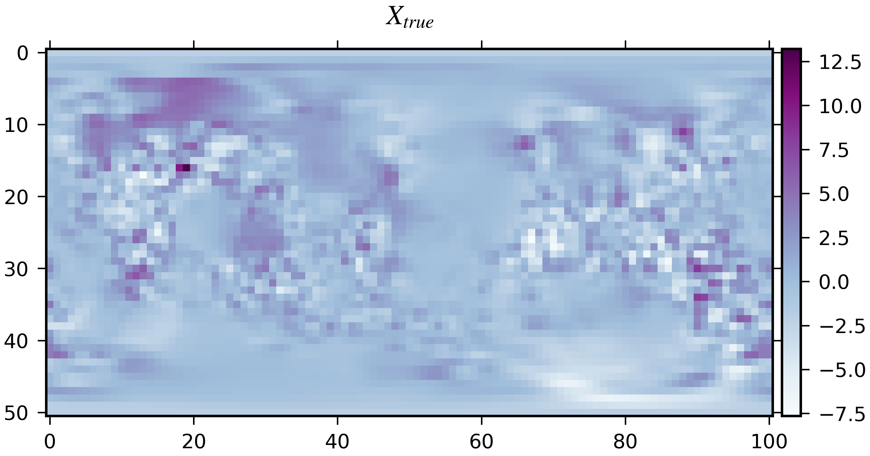
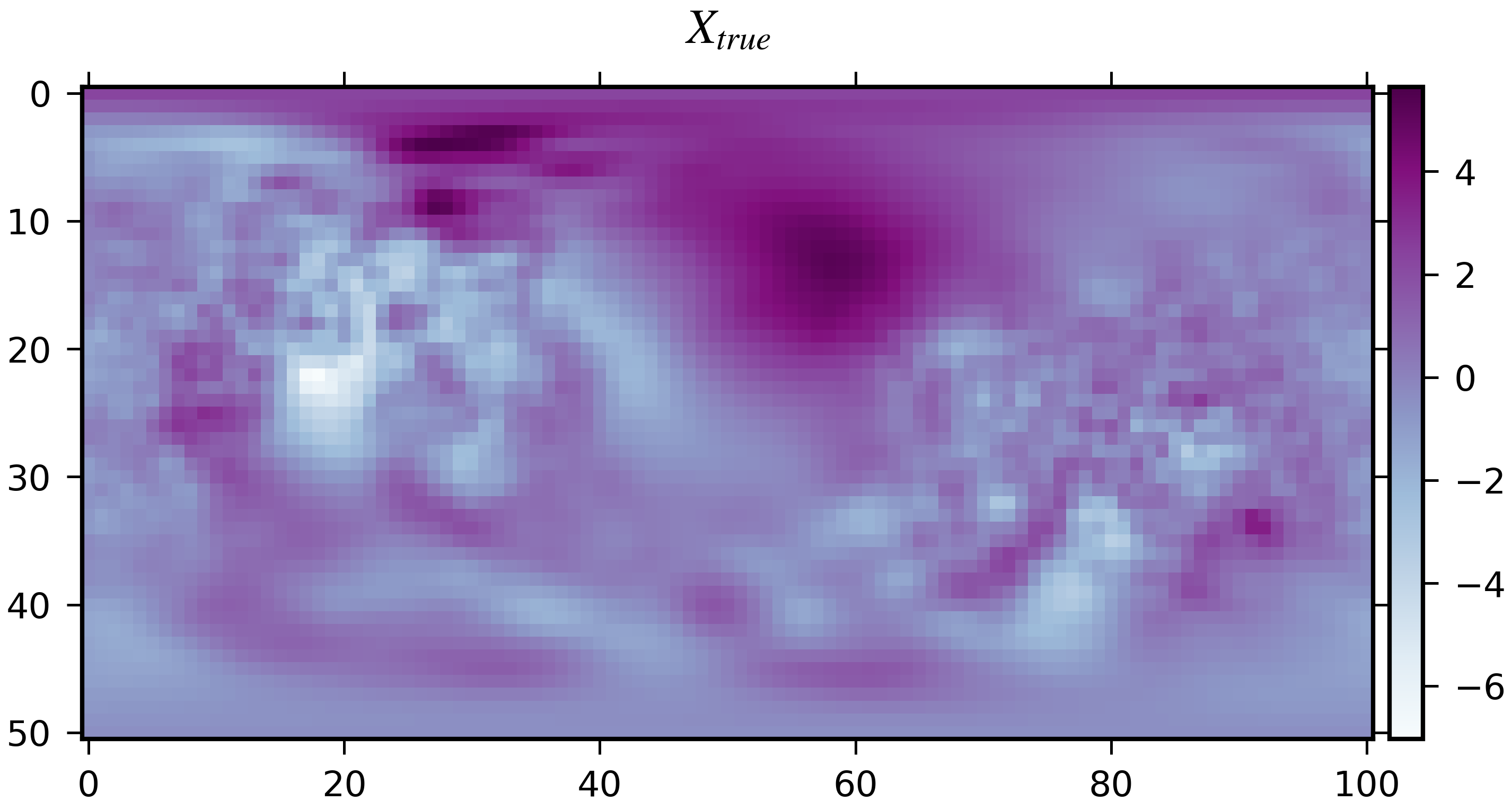
Figure 8: Two realizations of the random field produced by the model of “truth”.
Left: $\mu_{\rm NSL}=1$, Right: $\mu_{\rm NSL}=3$.
x-axis: longitude index, y-axis: co-latitude index.

H.5 Local stationarity

The (random) local spectra $f_{\ell}$ defined above in this Appendix give rise to a locally stationary random field $\xi(x)$ if $\varkappa\approx 1$ (low non-stationarity strength) or $\mu_{\rm NSL}\gg 1$ (large non-stationarity length), cf. Appendix E.

Indeed, if $\varkappa\approx 1$, the parameter fields are nearly constants in space, see Eq.(65). Therefore, the spatial variability in the local spectrum $f_{\ell}(x)$ is small, implying local stationarity given that $\mu_{\rm NSL}\geq 1$.

If $\mu_{\rm NSL}\gg 1$, the non-stationarity length $\Lambda_{\rm NSL}$ (Eq.(68)) is much larger than the median local length scale $\lambda_{\rm add}+\lambda_{\rm mult}$ implying local stationarity according to Appendix E.

References

- Asch et al. [2016] M. Asch, M. Bocquet, and M. Nodet. Data assimilation: methods, algorithms, and applications. SIAM, 2016.
- Berre and Desroziers [2010] L. Berre and G. Desroziers. Filtering of background error variances and correlations by local spatial averaging: A review. Mon. Weather Rev., 138(10):3693–3720, 2010.
- Berre et al. [2015] L. Berre, H. Varella, and G. Desroziers. Modelling of flow-dependent ensemble-based background-error correlations using a wavelet formulation in 4D-Var at Météo-France. Q. J. Roy. Meteorol. Soc., 141(692):2803–2812, 2015.
- Bonavita et al. [2016] M. Bonavita, E. Hólm, L. Isaksen, and M. Fisher. The evolution of the ECMWF hybrid data assimilation system. Quart. J. Roy. Meteor. Soc., 142(694):287–303, 2016.
- Boyles and Katzfuss [2021] W. Boyles and M. Katzfuss. Ensemble Kalman filter updates based on regularized sparse inverse Cholesky factors. Monthly Weather Review, 149(7):2231–2238, 2021.
- Bruinsma et al. [2022] W. P. Bruinsma, M. Tegnér, and R. E. Turner. Modelling non-smooth signals with complex spectral structure. In International Conference on Artificial Intelligence and Statistics, pages 5166–5195. PMLR, 2022.
- Buehner et al. [2013] M. Buehner, J. Morneau, and C. Charette. Four-dimensional ensemble-variational data assimilation for global deterministic weather prediction. Nonlin. Process. Geophys., 20(5):669–682, 2013.
- Dahlhaus [1997] R. Dahlhaus. Fitting time series models to nonstationary processes. Ann. Stat., 25(1):1–37, 1997.
- Driscoll and Healy [1994] J. R. Driscoll and D. M. Healy. Computing Fourier transforms and convolutions on the 2-sphere. Advances in applied mathematics, 15(2):202–250, 1994.
- Fisher [2003] M. Fisher. Background error covariance modelling. Proc. ECMWF Semin. on recent developments in data assimilation for atmosphere and ocean, 8-12 September 2003, pages 45–64, 2003.
- Furrer and Bengtsson [2007] R. Furrer and T. Bengtsson. Estimation of high-dimensional prior and posterior covariance matrices in Kalman filter variants. J. Multivar. Anal., 98(2):227–255, 2007.
- Gage and Nastrom [1986] K. S. Gage and G. D. Nastrom. Theoretical interpretation of atmospheric wavenumber spectra of wind and temperature observed by commercial aircraft during GASP. Journal of Atmospheric Sciences, 43(7):729–740, 1986.
- Gaspari and Cohn [1999] G. Gaspari and S. E. Cohn. Construction of correlation functions in two and three dimensions. Quart. J. Roy. Meteor. Soc., 125(554):723–757, 1999.
- Goodfellow et al. [2016] I. Goodfellow, Y. Bengio, and A. Courville. Deep learning. MIT press, 2016.
- Gryvill and Tjelmeland [2023] H. Gryvill and H. Tjelmeland. A sparse matrix formulation of model-based ensemble Kalman filter. Statistics and Computing, 33(3):63, 2023.
- Heaton et al. [2014] M. Heaton, M. Katzfuss, C. Berrett, and D. Nychka. Constructing valid spatial processes on the sphere using kernel convolutions. Environmetrics, 25(1):2–15, 2014.
- Higdon et al. [1999] D. Higdon, J. Swall, and J. Kern. Non-stationary spatial modeling. Bayes. Statist., 6(1):761–768, 1999.
- Hou et al. [2021] E. Hou, E. Lawrence, and A. O. Hero. Penalized ensemble Kalman filters for high dimensional non-linear systems. PloS one, 16(3):e0248046, 2021.
- Houtekamer and Zhang [2016] P. L. Houtekamer and F. Zhang. Review of the ensemble Kalman filter for atmospheric data assimilation. Monthly Weather Review, 144(12):4489–4532, 2016.
- Kakihara [1997] Y. Kakihara. Multidimensional second order stochastic processes. World Scientific, 1997.
- Kasanickỳ et al. [2015] I. Kasanickỳ, J. Mandel, and M. Vejmelka. Spectral diagonal ensemble Kalman filters. Nonlinear Processes in Geophysics, 22(4):485–497, 2015.
- Keydana [2023] S. Keydana. Deep Learning and Scientific Computing with R torch. CRC Press, 2023.
- Kingma and Ba [2014] D. P. Kingma and J. Ba. Adam: A method for stochastic optimization. arXiv preprint arXiv:1412.6980, 2014.
- Ledoit and Wolf [2004] O. Ledoit and M. Wolf. A well-conditioned estimator for large-dimensional covariance matrices. J. Multivar. Anal., 88(2):365–411, 2004.
- Lemos and Sansó [2009] R. T. Lemos and B. Sansó. A spatio-temporal model for mean, anomaly, and trend fields of North Atlantic sea surface temperature. Journal of the American Statistical Association, 104(485):5–18, 2009.
- Li and Zhu [2020] Y. Li and Z. Zhu. Spatio-temporal modeling of global ozone data using convolution. Japanese Journal of Statistics and Data Science, 3(1):153–166, 2020.
- Lorenc [2017] A. C. Lorenc. Improving ensemble covariances in hybrid variational data assimilation without increasing ensemble size. Quart. J. Roy. Meteor. Soc., 143(703):1062–1072, 2017.
- Lorenc et al. [2014] A. C. Lorenc, N. E. Bowler, A. M. Clayton, S. R. Pring, and D. Fairbairn. Comparison of hybrid-4DEnVar and hybrid-4DVar data assimilation methods for global NWP. Mon. Weather Rev., 143(2015):212–229, 2014.
- Mallat et al. [1998] S. Mallat, G. Papanicolaou, and Z. Zhang. Adaptive covariance estimation of locally stationary processes. The annals of Statistics, 26(1):1–47, 1998.
- Marinucci and Peccati [2011] D. Marinucci and D. Peccati. Random Fields on the Sphere. Cambridge University Press, 2011.
- Ménétrier et al. [2015] B. Ménétrier, T. Montmerle, Y. Michel, and L. Berre. Linear filtering of sample covariances for ensemble-based data assimilation. Part I: optimality criteria and application to variance filtering and covariance localization. Mon. Weather Rev., 143(5):1622–1643, 2015.
- Pannekoucke et al. [2007] O. Pannekoucke, L. Berre, and G. Desroziers. Filtering properties of wavelets for local background-error correlations. Quart. J. Roy. Meteorol. Soc., 133(623):363–379, 2007.
- Paszke et al. [2019] A. Paszke, S. Gross, F. Massa, A. Lerer, J. Bradbury, G. Chanan, T. Killeen, Z. Lin, N. Gimelshein, L. Antiga, A. Desmaison, A. Kopf, E. Yang, Z. DeVito, M. Raison, A. Tejani, S. Chilamkurthy, B. Steiner, L. Fang, J. Bai, and S. Chintala. Pytorch: An imperative style, high-performance deep learning library. In H. Wallach, H. Larochelle, A. Beygelzimer, F. d'Alché-Buc, E. Fox, and R. Garnett, editors, Advances in Neural Information Processing Systems 32, pages 8024–8035. Curran Associates, Inc., 2019. URL http://papers.neurips.cc/paper/9015-pytorch-an-imperative-style-high-performance-deep-learning-library.pdf.
- Priestley [1965] M. B. Priestley. Evolutionary spectra and non-stationary processes. Journal of the Royal Statistical Society. Series B (Methodological), 27(2):204–237, 1965.
- Searle and Khuri [2017] S. R. Searle and A. I. Khuri. Matrix algebra useful for statistics. John Wiley & Sons, 2017.
- Sham Bhat et al. [2012] K. Sham Bhat, M. Haran, R. Olson, and K. Keller. Inferring likelihoods and climate system characteristics from climate models and multiple tracers. Environmetrics, 23(4):345–362, 2012.
- Skauvold and Eidsvik [2019] J. Skauvold and J. Eidsvik. Parametric spatial covariance models in the ensemble Kalman filter. Spatial statistics, 29:226–242, 2019.
- Szegő [1939] G. Szegő. Orthogonal polynomials. American Mathematical Soc., 1939.
- Tobar et al. [2015] F. Tobar, T. D. Bui, and R. E. Turner. Learning stationary time series using Gaussian processes with nonparametric kernels. Advances in neural information processing systems, 28, 2015.
- Trenberth and Solomon [1993] K. E. Trenberth and A. Solomon. Implications of global atmospheric spatial spectra for processing and displaying data. Journal of climate, 6(3):531–545, 1993.
- Tsyrulnikov and Rakitko [2017] M. Tsyrulnikov and A. Rakitko. A hierarchical Bayes ensemble Kalman filter. Physica D, 338:1–16, 2017.
- Tsyrulnikov and Rakitko [2019] M. Tsyrulnikov and A. Rakitko. Impact of non-stationarity on hybrid ensemble filters: A study with a doubly stochastic advection-diffusion-decay model. Quart. J. Roy. Meteorol. Soc., 145(722):2255–2271, 2019.
- Tsyrulnikov et al. [2019] M. Tsyrulnikov, P. Svirenko, D. Gayfulin, M. Gorbunov, and A. Uspensky. Development of the operational meteorological data assimilation system in the Hydrometcenter of Russia (in Russian). Hydrometeorological Research and Forecasting, (4(374)):112–126, 2019.
- Ueno and Tsuchiya [2009] G. Ueno and T. Tsuchiya. Covariance regularization in inverse space. Q. J. Roy. Meteorol. Soc., 135(642):1133–1156, 2009.
- Wieczorek and Meschede [2018] M. A. Wieczorek and M. Meschede. SHTools: Tools for working with spherical harmonics. Geochemistry, Geophysics, Geosystems, 19(8):2574–2592, 2018.