Propagation of Quantum Information in Tree Networks: Noise Thresholds for Infinite Propagation

Abstract

We study quantum networks with tree structures, where information propagates from a root to leaves: at each node in the network, the received qubit unitarily interacts with fresh ancilla qubits, and then each qubit is sent through a noisy channel to a different node in the next level. As the tree’s depth grows, there is a competition between the decay of quantum information due to the noisy channels and the additional protection against noise that is achieved by further delocalizing information. In the classical setting, where each node just copies the input bit into multiple output bits, this model has been studied as the broadcasting or reconstruction problem on trees, which has broad applications. In this work, we study the quantum version of this problem, where the encoder at each node is a Clifford unitary that encodes the input qubit in a stabilizer code. Such noisy quantum trees, for instance, provide a useful model for understanding the effect of noise within the encoders of concatenated codes. We prove that above certain noise thresholds, which depend on the properties of the code such as its distance, as well as the properties of the encoder, information decays exponentially with the depth of the tree. On the other hand, by studying certain efficient decoders, we prove that for codes with distance $d\geq 2$ and for sufficiently small (but non-zero) noise, classical information and entanglement propagate over a noisy tree with infinite depth. Indeed, we find that this remains true even for binary trees with certain 2-qubit encoders at each node, which encode the received qubit in the binary repetition code with distance $d=1$.

I Introduction

Overcoming noise and decoherence in quantum systems is the biggest challenge for quantum information technology. Understanding how these undesirable phenomena affect storage, communication and processing of quantum information is a problem with broad interest Preskill (2018). Beyond these applications, understanding the competition between entanglement generation and noise in quantum circuits is a fundamental problem in many-body physics that has attracted significant attention in recent years Gullans and Huse (2020a, b); Skinner et al. (2019); Li et al. (2019).

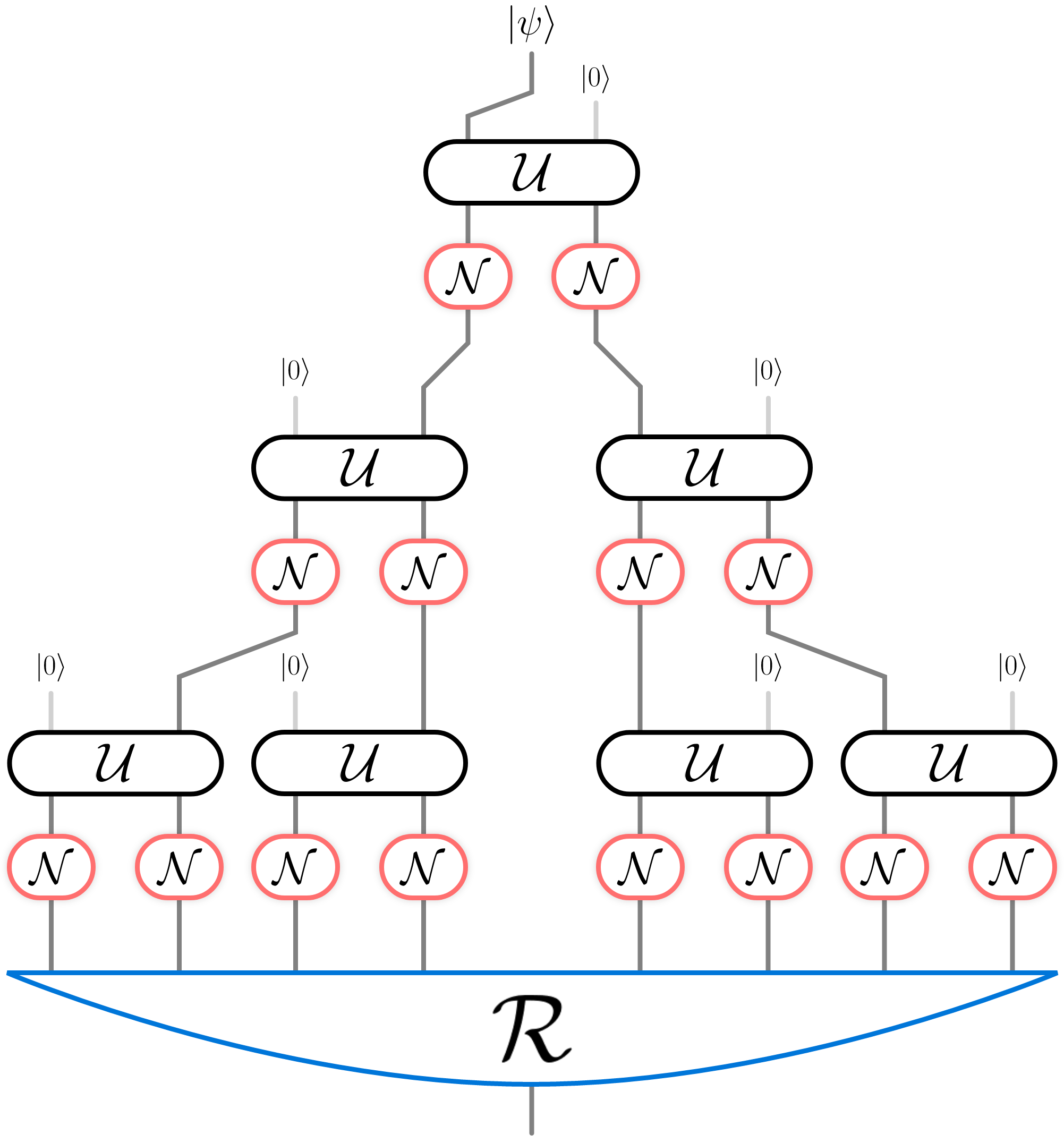
Figure 1: Noisy Quantum Tree– Here, the input qubit at the root of the tree is in unknown state $\ket{\psi}$, each $\mathcal{U}$ is a unitary transformation that couples an input qubit to a fresh ancilla qubit initially prepared in state $|0\rangle$, and $\mathcal{N}$ is a noise process (Time flows from top to bottom). $\mathcal{R}$ represents a decoding process that takes all the leaf qubits and approximately reconstructs the root state. The illustrated quantum tree has depth $T=3$.

Classically, the study of noisy circuits traces back to von Neumann when he proved the first threshold theorem for fault-tolerant computation using noisy elements Von Neumann (1956). In subsequent decades, Pippenger and others further developed this into a theory of noisy circuits Pippenger (1985, 1988); Benjamini et al. (1998); Kesten and Stigum (1966). A particularly interesting and useful model for the propagation of classical information is broadcasting on noisy trees (see, e.g., Evans et al. (2000); Lyons and Peres (2016)). A broad class of classical processes – both natural and artificial – can be modeled as such trees. Applications include broadcasting networks, reconstruction in genetics, and Ising models in statistical physics Evans et al. (2000); Mossel (2001); Mossel and Peres (2003); Lyons and Peres (2016).

Here we consider a basic version of this problem: at a distinguished node, called the root of the tree, a bit of information is received and then it is sent to $b$ other nodes in the next level. Then, each node in the next level sends the received bit to $b$ other nodes in the next level, and so on. Now suppose each link between the nodes at two successive levels is noisy, so that the bit is flipped with probability $p$. Suppose the tree has depth $T$. Let $p(\textbf{x}_{T}|\textbf{x}_{0})$ be the probability that at level $T$ the leaves are in bit-string $\textbf{x}_{T}\in\{0,1\}^{b^{T}}$, given that the input bit at the root is $\textbf{x}_{0}\in\{0,1\}$. A basic interesting question here is as $T\rightarrow\infty$, whether the leaves remain correlated with the input bit or not. We can formulate this in terms of the total variation distance of the distributions associated to inputs $\textbf{x}_{0}=0$ and $\textbf{x}_{0}=1$, i.e.,

$$\frac{1}{2}\sum_{\textbf{x}_{T}\in\{0,1\}^{b^{T}}}\Big{|}p(\textbf{x}_{T}|\textbf{x}_{0}=0)-p(\textbf{x}_{T}|\textbf{x}_{0}=1)\Big{|}\ .$$ (1)

In particular, does this distance vanish in the limit $T\rightarrow\infty$? If so, then it will be impossible to determine the value of the input bit at the root by looking at the output bits at the leaves.

In a paper Evans et al. (2000) published in 2000, Evans et. al showed that for infinite $b$-ary trees and, more generally, for trees with branching number $b$ and with bit-flip probability $p$, if $b<(1-2p)^{-2}$ then the total variation distance in Eq.(1) vanishes exponentially fast with $T$, whereas it remains non-zero for $b>(1-2p)^{-2}$, even in the limit $T\rightarrow\infty$. In other words, there is a critical noise threshold

$$p_{\text{th}}=\frac{1}{2}\Big{(}1-\frac{1}{\sqrt{b}}\Big{)}\ .$$ (2)

For $p<p_{\text{th}}$, information about the input never fully disappears in the output, even as $T\rightarrow\infty$. Whereas for $p_{\text{th}}<p\leq 1/2$, the output of the tree is asymptotically uncorrelated with the input.

In this paper, we study the quantum version of this problem. Clearly, in the quantum setting, due to the no-cloning Wootters and Zurek (1982) and no-broadcasting Barnum et al. (1996) theorems, it is not possible to copy quantum information. Then, a natural way to generalize the classical problem to the quantum setting is to assume that at each node the received qubit unitarily interacts with one or multiple ancilla qubits initially prepared in a fixed pure state $|0\rangle$, and then each qubit is transmitted to a node in the next layer through a noisy single-qubit channel (see Fig. 1). The unitaries at different nodes can be identical or different, and possibly random.

Due to the noise in the circuit, as information propagates from the root to the leaves of the tree, at each step it partially decays. At the same time, the unitary transformation at each node “delocalizes” information in a single qubit into multiple qubits. Even though this unitary transformation may not necessarily be the encoder of an error-correcting code, the intuition from the theory of quantum error correction suggests that this delocalization of information can protect information against local noise. Hence, as the tree depth grows, there is a competition between the effect of noise and the protection against such noise achieved by further delocalization of information.

$$\Qcircuit@C=1em@R=1em{\lstick{\ket{\psi}}&\qw\qw\gate{H}\ctrl{+2}\qw\gate{\mathcal{N}}\gate{H}\ctrl{+1}\gate{\mathcal{N}}\qw\\ \lstick{\ket{0}}\qw\oplus\gate{\mathcal{N}}\qw\\ \lstick{\ket{0}}\qw\oplus\qw\gate{\mathcal{N}}\gate{H}\ctrl{+1}\gate{\mathcal{N}}\qw\\ \lstick{\ket{0}}\qw\oplus\gate{\mathcal{N}}\qw\gategroup{1}{3}{3}{5}{1.6em}{--}\\ }\large$$

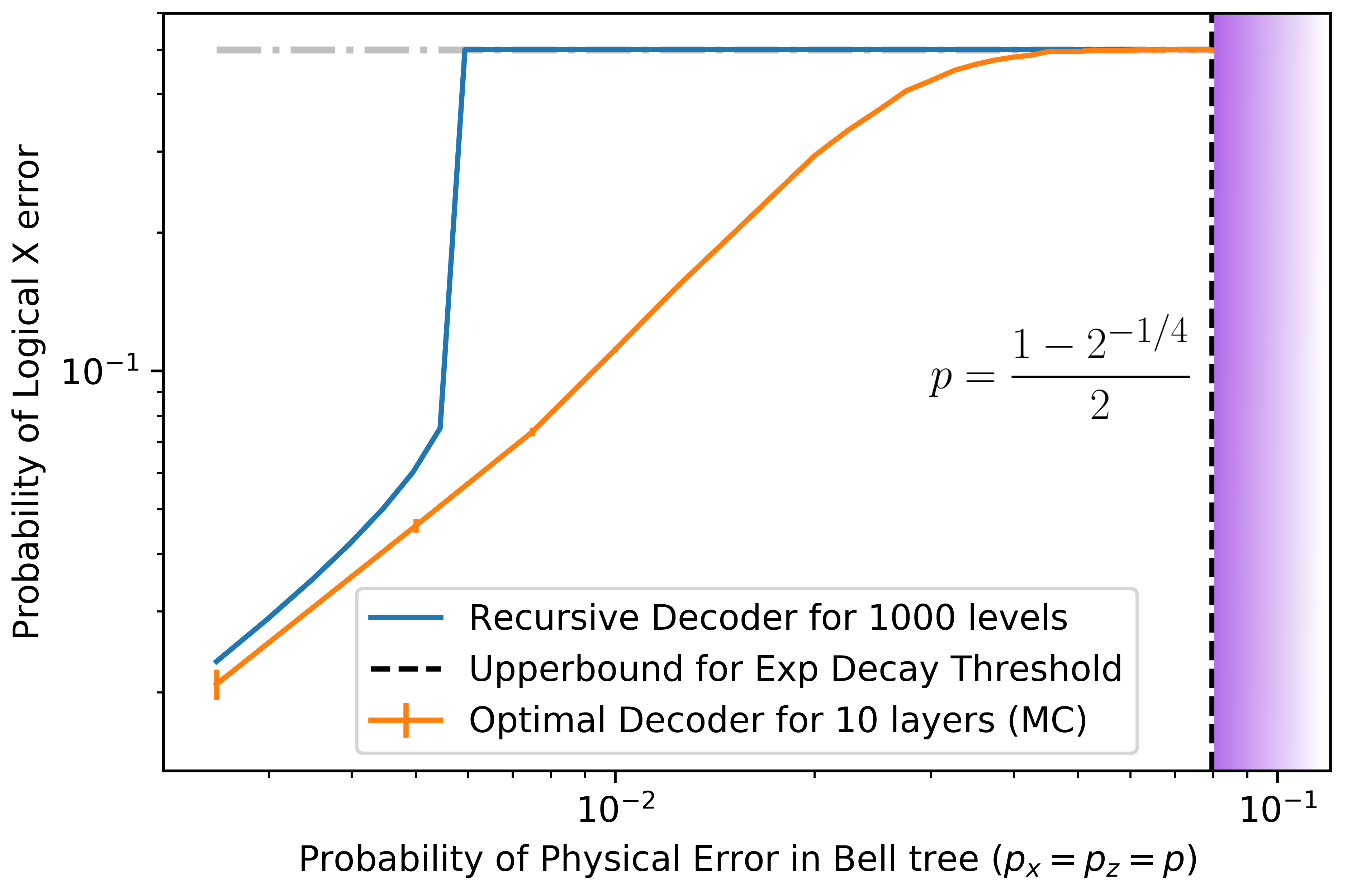
Figure 2: The Bell Tree – The top figure presents a binary tree, which we call a Bell tree, with depth $T=2$. Here, we assume that the single-qubit channel $\mathcal{N}$ consists of independent bit-flip and phase-flip channels which apply $X$ and $Z$ errors with probability $p_{x}=p_{z}=p$. The plot describes the probability of error after decoding, i.e., the probability of logical error. Using the fact that the Bell tree has logical subtrees with branching number $\sqrt{2}$, we show that for $p>(1-2^{-1/4})/2\sim 8\%$, information decays exponentially with depth $T$ (see Sec. III). Therefore, the probability of $X$ logical error for the infinite tree is $1/2$ (the same holds for the probability of logical $Z$ errors). The blue curve corresponds to the probability of logical $X$ error for a Bell tree of depth $T=1000$ after applying an efficient decoder introduced in Sec.VI, which uses a recursive scheme with 2 reliability bits. The threshold for this decoder is around $p_{x}=p_{z}\sim 0.05\%$. The orange curve corresponds to the logical $X$ error after applying the optimal decoder for the Bell tree of depth $T=10$, which is implemented via the belief propagation algorithm presented in Sec.VII. This plot suggests that the actual noise threshold for infinite propagation is below $4\%$.

Fig. 2 presents a simple example of this problem for a tree of depth $T=2$, where at each node the received qubit goes through a Hadamard gate and then interacts with a fresh ancilla qubit via a CNOT. We call this the Bell tree of depth $T=2$, because the unitary transformation at each node (the dotted box in Fig. 2) transforms the computational basis of two qubits to the so-called Bell basis (note that $T=2$ Bell tree can be interpreted as the encoder of the generalized Shor code [[4,1,2]]). The “quantum code” defined by this two-qubit encoder is the repetition code and has distance $d=1$, which means it cannot correct or detect general single-qubit errors.

Nevertheless, we prove that for noise below a certain threshold, classical information and entanglement propagate over the Bell tree with depth $T\rightarrow\infty$ (see Fig. 2). In particular, we show that if $Z$ and $X$ errors occur independently with probability $p_{z}=p_{x}<\sim 0.5\%$, then entanglement with a hypothetical reference qubit that is initially entangled with the input, survives over the infinite tree. To achieve this we introduce and analyze a novel decoder that during decoding augments every qubit with two reliability bits to recursively decode and recover the input state (see the decoder in Fig.15). It is worth noting that in the classical broadcasting problem discussed above, the threshold in Eq.(2) can be achieved via majority voting on the leaves of the tree Evans et al. (2000). In the quantum setting, on the other hand, the decoder is more complicated. Indeed, in contrast to the classical case, even in the absence of noise, it is impossible to obtain any information about the input state without having access to $\approx\sqrt{2^{T}}$ qubits (see Sec.III.4).

We also rigorously prove that for

$$p_{z}=p_{x}>\frac{1-2^{-1/4}}{2}\approx 8\%\ ,$$ (3)

classical information, e.g., as quantified by the trace distance or mutual information, decays exponentially in the tree, and in the limit $T\rightarrow\infty$ the output of the tree channel becomes independent of the input. Numerical analysis of the Bell tree of depth $T=10$, which is performed via a belief propagation algorithm discussed in Sec.VII, suggests that the actual threshold is close below $4\%.$

It is worth comparing this tree with a similar tree obtained by removing the Hadamard gates, which is essentially equivalent to the classical binary tree. While removing Hadamard does not change the code defined at each node, it drastically affects the propagation of information in the noisy quantum tree: any non-zero probability of $Z$ errors results in an exponential decay of information encoded in $X$ and $Y$ basis of the input qubit and in the limit $T\rightarrow\infty$, the output of the tree is always fully dephased in the computational basis.

Similar to the classical case, the study of the properties of noisy quantum trees is expected to be useful for broad applications. Specifically, such networks are relevant in the context of quantum computing and quantum communications with faulty components. E.g., they describe the effect of noise within the encoder of concatenated codes Rahn et al. (2002); Poulin (2006). Also, they describe the effect of noise on circuits that prepare tree tensor network states Shi et al. (2006) on quantum computers. Noisy quantum trees also provide a natural model for the physical process in which a particle enters a cold environment and randomly interacts with other particles in the environment which are initially in a pure state. Other possible applications of this model can be in, e.g., the study of quantum chaos and scrambling Roberts and Stanford (2013); Almheiri et al. (2015); Pastawski et al. (2015).

I.1 Overview of Results

In this paper, we will mainly focus on the stabilizer trees whose vertices correspond to the same encoder of a stabilizer code, and whose edges are subject to the same single-qubit Pauli noise (see Sec. II). In the following, we summarize the results presented in each section:

• In Sec. III we prove an upperbound on the distinguishability of the output states at the leaves of the tree, as quantified by the trace distance, and show that for noise above a certain threshold it decays exponentially fast with the tree depth $T$ (see Propositions 1, 2 and 3).

• In Sec. IV we study a decoding strategy based on local recovery, where one recursively decodes blocks of qubits corresponding to the encoder at each node of the tree. While it is sub-optimal, using this strategy we can rigorously prove the existence of a non-zero noise threshold in the case of codes with distance $d\geq 3$.

• In Sec. V we consider codes with distance $d=2$, which cannot correct single-qubit errors in unknown locations. In this case the local recursive recovery approach of Sec. IV, does not yield a non-zero threshold for the infinite tree. To overcome this, we consider a modification of this scheme where at each step one passes a single classical “reliability” bit to the next level. We rigorously prove and numerically demonstrate that this approach achieves a non-zero noise threshold for the infinite tree.

• In Sec. VI we study the Bell tree (see Fig. 2), that corresponds to a 2-qubit code with distance $d=1$. Such codes cannot even detect general single-qubit errors. Nevertheless, we rigorously prove and numerically demonstrate the existence of a non-zero threshold. To achieve this we introduce and analyze an efficient decoder, which is a simple modification of the recursive local recovery where at each step two reliability bits are sent to the next level.

• In Sec. VII we describe an optimal and efficient recovery strategy for stabilizer trees that involves a belief propagation algorithm on classical syndrome data. This allows us to numerically study the decay of information in any stabilizer tree with Pauli noise.

• Finally, in Sec. VIII we show that by fully dephasing qubits at all levels, the stabilizer tree problem can be mapped to an equivalent fully classical problem about propagation of information on a classical tree with correlated noise.

I.2 Previous Related Works

The study of noisy quantum circuits goes back to the pioneering work of Peter Shor in 1995 Shor (1995), who discovered quantum error-correcting codes. Shortly after, the threshold theorem for fault-tolerant quantum computing was established Aharonov and Ben-Or (2008); Knill et al. (1996). In particular, Knill et al Knill et al. (1996) used codes obtained by concatenating codes with distance $d\geq 3$ to establish the presence of a non-zero noise threshold below which arbitrarily long quantum computation is possible (see also Gottesman (2014); Chamberland et al. (2016) for more recent works).

It is worth noting that there are some crucial differences between the standard settings of fault-tolerant quantum computation and the setup considered in this paper, e.g., in Fig.1. On one hand, we assume access to noiseless ancilla qubits, and a noiseless decoder that acts on all the output qubits collectively—resources that are not available in the context of fault-tolerant quantum computation. On the other hand, in contrast to the standard setup for fault-tolerant quantum computation, we do not allow measurements, classical communication, and error correction in the middle of the (infinite) tree network. Furthermore, because of the tree structure, the gates cannot couple two “data” qubits together; they only couple a data qubit to fresh ancilla qubits prepared in a fixed state. In conclusion, although non-zero noise thresholds appear in both settings, the exact value of these thresholds are not necessarily related.

Here, we mention a few other related works in the context of fault-tolerant quantum computation. Aharonov studied noise-induced phase transitions in the propagation of entanglement in noisy quantum circuits Aharonov (2000). Harrow and Nielsen placed an upper bound of $0.74$ for fault-tolerance threshold Harrow and Nielsen (2003) with 2-local gates. Razbarov Razborov (2004) improved this upper bound to $1-1/k$ for $k$-local gates. Kempe et al. Kempe et al. (2010) further improved this to $1-\Theta(1/\sqrt{k})$ by studying the evolution of the Hilbert-Schmidt distance between two inputs to a circuit, but limiting to the distinguishability of a single (or a few) output qubits. Similarly, the effect of noise in Haar-random circuits has been recently studied Dalzell et al. (2021); Deshpande et al. (2022); Dalzell et al. (2022).

II The setup: Noisy Quantum Trees

II.1 General Case

Suppose at each node of a full $b$-ary tree a qubit arrives and interacts with $b-1$ ancillary qubits initially prepared in a fixed state $|0\rangle$ via a unitary transformation $U$, and then each qubit is sent to a different node in the next level. The overall process at each node can be described as an isometry $V:\mathbb{C}^{2}\rightarrow(\mathbb{C}^{2})^{\otimes b}$ defined by

$$V|\psi\rangle=U(|\psi\rangle|0\rangle^{\otimes(b-1)})\ .$$ (4)

The image of $V$ defines a 2-dimensional code subspace in a $2^{b}$-dimensional Hilbert space of $b$ qubits. Applying the above process recursively $T$ times, we obtain a chain of encoded states

$$|\psi\rangle\rightarrow|\psi_{1}\rangle\rightarrow\cdots\rightarrow|\psi_{T}\rangle\ ,$$ (5)

where the state at level $k+1$ is obtained via the relation

$$|\psi_{k+1}\rangle=V^{\otimes b^{k}}|\psi_{k}\rangle\ .$$ (6)

Then, the overall process can be described by the isometry

$$V_{T}=\prod_{j=0}^{T-1}V^{\otimes{b}^{j}}=V^{\otimes b^{T-1}}\cdots V^{\otimes{b}^{2}}V^{\otimes b}V\ ,$$ (7)

that encodes 1 qubit in

$$N=b^{T}$$ (8)

qubits. We denote the corresponding quantum channel by $\mathcal{V}_{T}$, where $\mathcal{V}_{T}(\rho)=V_{T}\rho V_{T}$.

In the language of quantum error-correcting codes, the above process defines a concatenated code Gottesman (1997); Poulin (2006). In this context, one often ignores the noise within the encoder. However, we are interested to understand how such noise would affect the output state. Therefore, we assume that after each encoder $V$, the output qubits go through noisy channels (see Fig.1). Furthermore, we assume the noise is independent and identically distributed (i.i.d.) on all qubits and the noise on each qubit is described by the single-qubit channel $\mathcal{N}$. Then, the noisy tree can be described by the quantum channel

$$\mathcal{E}_{T}=\prod_{j=0}^{T-1}\mathcal{N}^{\otimes b^{j+1}}\circ\mathcal{V}^{\otimes b^{j}}\ .$$ (9)

For example, the circuit in Figure 1 corresponds to $\mathcal{E}_{3}$. Channel $\mathcal{E}_{T}$ can also be defined recursively as

$$\mathcal{E}_{T}=\mathcal{E}^{\otimes b}_{T-1}\circ\mathcal{N}^{\otimes b}\circ\mathcal{V}=\widetilde{\mathcal{E}}^{\otimes b}_{T-1}\circ\mathcal{V}\ ,$$ (10)

where

$$\widetilde{\mathcal{E}}_{T}=\mathcal{E}_{T}\circ\mathcal{N}\ ,$$ (11)

corresponds to the noisy tree where the noise is also applied on the input qubit prior to the first encoder. Note that the presence of this single-qubit channel at the root does not affect the noise threshold for transmitting classical information in the infinite tree.

II.2 Stabilizer Trees with Pauli Noise

In this paper, we mainly assume that the single-qubit noise channel $\mathcal{N}$ is a Pauli channel. Specifically, we will be interested in the case of independent $X$ and $Z$ errors, i.e.,

$$\mathcal{N}=\mathcal{N}_{x}\circ\mathcal{N}_{z}=\mathcal{N}_{z}\circ\mathcal{N}_{x}\ ,$$ (12)

where

$$\mathcal{N}_{x}(\rho) =(1-p_{x})\rho+p_{x}X\rho X,$$ (13a)

$$\mathcal{N}_{z}(\rho) =(1-p_{z})\rho+p_{z}Z\rho Z$$ (13b)

are, respectively, bit-flip and phase-flip channels.

We also assume the encoder unitary $U$ in Eq.(4) is a Clifford unitary, such that for all $P\in\mathcal{P}_{b}=\{\eta I,\eta X,\eta Y,\eta Z:\eta=\pm 1,\pm i\}^{\otimes b}$, $UPU^{\dagger}\in\mathcal{P}_{b}$. Recall that any Clifford unitary can be realized by composing CNOT, Hadamard and Phase gates Gottesman (1997); Nielsen and Chuang (2002). The code defined by this encoder is a stabilizer code with the stabilizer generators

$$UZ_{j}U^{\dagger}\ \ \ :j=2,\cdots,b\ ,$$ (14)

where $Z_{j}$ denotes the Pauli $Z$ operator on qubit $j$ tensor product with identity operators on the other qubits Gottesman (1997); Nielsen and Chuang (2002). Given any stabilizer code, there exists an encoder $U$ satisfying the additional property that it has a logical operator $Z_{L}$, such that $Z_{L}V=VZ$ and $Z_{L}\in\langle iI,Z\rangle^{\otimes b}$, i.e., $Z_{L}$ can be written as a tensor product of the identity and Pauli $Z$ operators, up to a global phase. Following Gottesman (1997); Nielsen and Chuang (2002) we refer to such an encoder as a standard encoder.

A nice feature of stabilizer codes is the existence of a simple error-correction scheme for correcting Pauli errors: suppose after encoding the qubits are subjected to Pauli errors, which in general can be correlated for different qubits. Then, the optimal recovery of the (unknown) input state $|\psi\rangle$ can be achieved by measuring the stabilizers of the code, which can be realized by first applying the inverse of the Clifford unitary $U$, and then measuring all the ancilla qubits in the $Z$ basis. Then, based on the outcomes of these measurements, one applies one of the Pauli operators $X,Y,Z$, or the identity operator on the data qubit to correct the error and recover the state $|\psi\rangle$ (the choice of the Pauli operator depends on the inferred distribution of Pauli errors given the syndrome information).

We study the propagation of information through these noisy stabilizer trees by considering recovery channels (decoders) that process all the $b^{T}$ leaf qubits as the input, and then output a single (approximately) recovered qubit. Note that the optimal recovery channel $\mathcal{R}^{\rm opt}_{T}$ for the stabilizer tree $\mathcal{E}_{T}$ is the standard stabilizer recovery procedure noted earlier, but for the entire concatenated encoder unitary, $V_{T}$.

After performing the optimal recovery for the stabilizer codes with Pauli errors, the entire process can be described by a Pauli channel, as

$$\mathcal{R}^{\rm opt}_{T}\circ\mathcal{E}_{T}(\rho)=r^{I}_{T}\rho+r^{x}_{T}X\rho X+r^{y}_{T}Y\rho Y+r^{z}_{T}Z\rho Z\ ,$$ (15)

for arbitrary density operator $\rho$, where $r^{I}_{T},r^{X}_{T},r^{Y}_{T},r^{Z}_{T}\geq 0$.

II.2.1 CSS Codes with standard encoders

As an important special case, we consider the case of CSS (Calderbank-Shor-Steane) codes with standard encoders. CSS stabilizer codes on $b$ qubits are those whose stabilizer generators $UZ_{j}U^{\dagger}\ :j=2,\cdots,b$ belong to either $\langle iI,Z\rangle^{\otimes b}$, or $\langle iI,X\rangle^{\otimes b}$, i.e., can be written as the tensor product of the identity operators with only Pauli $Z$, or only Pauli $X$ operators Calderbank and Shor (1996); Steane (1996); Calderbank et al. (1997).

Every CSS code has a standard encoder $V$, defined by the property that there exist logical operators $Z_{L}$ and $X_{L}$, such that $Z_{L}V=VZ$ and $X_{L}V=VX$, and $Z_{L}\in\langle iI,Z\rangle^{\otimes b}$, $X_{L}\in\langle iI,X\rangle^{\otimes b}$. This property, in particular, implies that the concatenated code defined by the encoder $V_{T}$ in Eq.(7) is also a CSS code.

The fact that the stabilizer generators of a CSS code can be partitioned into two types containing only $Z$ or only $X$ Pauli operators simplifies the analysis of error correction. In particular, if $Z$ and $X$ errors are independent, such that $\mathcal{N}=\mathcal{N}_{x}\circ\mathcal{N}_{z}$, then after optimal error correction the overall channel can also be decomposed as a composition of a bit-flip and phase-flip channel as,

$$\mathcal{R}^{\text{opt}}_{T}\circ\mathcal{E}_{T}=\mathcal{Q}_{z}\circ\mathcal{Q}_{x}=\mathcal{Q}_{x}\circ\mathcal{Q}_{z}\ ,$$ (16)

where

$$\mathcal{Q}_{z}(\rho) =(1-q^{z}_{T})\rho+q^{z}_{T}Z\rho Z$$ (17a)

$$\mathcal{Q}_{x}(\rho) =(1-q^{x}_{T})\rho+q^{x}_{T}X\rho X\ .$$ (17b)

Note that this is a special case of Eq.(15) corresponding to $r_{T}^{x}=q_{T}^{x}(1-q_{T}^{z})$, $r_{T}^{z}=q_{T}^{z}(1-q_{T}^{x})$, and $r_{T}^{y}=q_{T}^{x}q_{T}^{z}$. We refer to $q^{x}_{T},q^{z}_{T}$ as probabilities of logical $X$ and $Z$ errors for the tree of depth $T$, respectively. These probabilities grow monotonically with the tree depth $T$ and are bounded by 1/2. Therefore, the limits of $T\rightarrow\infty$ of $q^{z}_{T}$ and $q^{x}_{T}$ exist and are denoted by $q^{z}_{\infty}$ and $q^{x}_{\infty}$, respectively.

III The noise threshold for exponential decay of information

In this section, we establish that if the noise is stronger than a certain threshold in noisy quantum trees, then information decays exponentially fast with the depth of the tree. First, we start with the special case of standard encoders and then in Sec.III.4 we present the general result that applies to general (Clifford) encoders. The results presented in Sec. III.1, III.2, and III.3 are proved in Sec. III.5 and III.6.

III.1 Stabilizer Trees with Standard Encoders

Consider trees with general stabilizer codes with standard encoders. Recall that the weight of an operator $P\in\mathcal{P}_{b}$, denoted by ${\rm weight}(P)$, is the number of qubits on which $P$ acts non-trivially, i.e., is not a multiple of the identity operator. In the following, $\|\cdot\|_{\diamond}$ denotes the diamond norm (see Appendix B.1 for the definition). We prove that,

Proposition 1.

Let $V:\mathbb{C}^{2}\rightarrow(\mathbb{C}^{2})^{\otimes b}$ be the encoder of a stabilizer code that encodes one qubit into $b$ qubits. Suppose for this encoder there exists a logical $Z$ operator $Z_{L}$, satisfying $VZ=Z_{L}V$, which can be written as the tensor product of Pauli $Z$ and identity operators $I$, i.e., $Z_{L}\in\langle iI,Z\rangle^{\otimes b}$ (any stabilizer code has an encoder with this property). Let

$$b_{z}={\rm weight}(Z_{L})$$ (18)

be the weight of $Z_{L}$. Suppose the noise channel $\mathcal{N}$ that defines the tree channel $\mathcal{E}_{T}$ in Eq.(9) is $\mathcal{N}=\mathcal{N}_{x}\circ\mathcal{N}_{z}$, where $\mathcal{N}_{x}$ and $\mathcal{N}_{z}$ are, respectively, the bit-flip and phase-flip channels. Let $p_{z}$ be the probability of $Z$ error in the phase-flip channel $\mathcal{N}_{z}$. Then,

$$\big{\|}\mathcal{E}_{T}-\mathcal{E}_{T}\circ\mathcal{D}_{z}\big{\|}_{\diamond}\leq{\sqrt{2}}\times\Big{[}\sqrt{b_{z}}\times|1-2p_{z}|\Big{]}^{T}\ ,$$ (19)

where $\mathcal{D}_{z}(\rho)=(\rho+Z\rho Z)/2$ is the fully dephasing channel.

Therefore, for $p_{z}$ in the interval $(1-{b_{z}}^{-\frac{1}{2}})/2<p_{z}<(1+{b_{z}}^{-\frac{1}{2}})/2$, in the limit $T\rightarrow\infty$ the channel $\mathcal{E}_{T}$ becomes a classical-quantum channel that transfers input information only in the $Z$ basis. Note that, in general, the logical operator $Z_{L}$ is not unique and the strongest bound is obtained for the logical operator with the minimum weight $b_{z}$. As we further explain in Sec.III.5, the main idea for proving this result, and the other similar bounds found in this section, is to consider the logical subtree defined by the sequence of logical operators in the tree (see Fig.3).

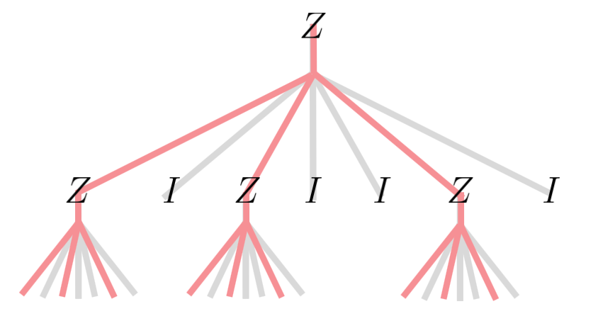
Figure 3: Illustration of the logical subtree – Here we consider a tree defined by a standard encoder of Steane-7 code. The highlighted subtree corresponds to the logical operator $Z_{L}=ZIZIIZI$, and is called a “logical subtree” in this paper. In this case, the logical subtree is a full 3-ary tree, whereas the original tree is a full 7-ary tree.

It is also worth emphasizing that in this proposition we are not comparing channel $\mathcal{E}_{T}$ with its noiseless version $\mathcal{V}_{T}$, which is more common in the context of noisy quantum circuits. Rather, we are comparing $\mathcal{E}_{T}$ with $\mathcal{E}_{T}\circ\mathcal{D}_{z}$, or equivalently with $\mathcal{E}_{T}\circ\mathcal{Z}$, where $\mathcal{Z}(\cdot)=Z(\cdot)Z$ is the channel that applies Pauli $Z$ on the input qubit. In particular, note that

$$\big{\|}\mathcal{E}_{T}-\mathcal{E}_{T}\circ\mathcal{D}_{z}\big{\|}_{\diamond}=\frac{1}{2}\big{\|}\mathcal{E}_{T}-\mathcal{E}_{T}\circ\mathcal{Z}\big{\|}_{\diamond}\ .$$ (20)

In the light of Helstrom’s theorem Helstrom (1969), this result can be understood in terms of the decay of distinguishability of states: suppose at the input of the tree we have one of the orthogonal states $\ket{\pm}=(\ket{0}\pm\ket{1})/\sqrt{2}$ with equal probabilities (this corresponds to sending a bit of classical information in the $X$ basis). Then, by looking at the output state at the tree’s leaves, we can successfully distinguish these two cases with the maximum success probability

$$P_{\text{success}} =\frac{1}{2}+\frac{||\mathcal{E}_{T}(|{+}\rangle\!\langle+|)-\mathcal{E}_{T}(|{-}\rangle\!\langle-|)||_{1}}{4}$$

$$\leq\frac{1}{2}+\frac{(\sqrt{b_{z}}|1-2p_{z}|)^{T}}{\sqrt{2}}\ ,$$ (21)

where $\|\cdot\|_{1}$ denotes the $l$-1 norm, the first equality follows from Helstrom’s theorem, and the inequality follows from the above proposition by noting that $Z|+\rangle=|-\rangle$ and the $l$-1 norm for any particular state is bounded by the diamond norm. We conclude that for input states corresponding to $X$ eigenstates, the distinguishability of states decays exponentially with the depth $T$ of the tree (the same holds true for $Y$ eigenstates as well).

III.2 CSS code trees with Standard Encoders

As mentioned in Sec.II.2.1 every CSS code has encoders that are standard for both $Z$ and $X$ directions. Therefore, for trees constructed from such encoders, we can apply this bound to both $Z$ and $X$ directions. Let $d_{z}$ and $d_{x}$ be the minimum weight of logical $Z$ and $X$ operators, respectively. Then, applying the triangle inequality, we find that the trace distance of the outputs of the channel $\mathcal{E}_{T}$ for an arbitrary input density operator $\rho$ and the maximally-mixed state is bounded by

$$\big{\|}\mathcal{E}_{T}(\rho)-\mathcal{E}_{T}(\frac{I}{2})\big{\|}_{1}\leq$$

$${\sqrt{2}}\times\Big{(}[\sqrt{d_{z}}|1-2p_{z}|]^{T}+[\sqrt{d_{x}}|1-2p_{x}|]^{T}\Big{)}\ .$$ (22)

Another useful way of characterizing the error in channel $\mathcal{E}_{T}$ is in terms of the probability of logical errors. Recall that for CSS codes with standard encoders and independent $Z$ and $X$ errors, the optimal error correction can be performed independently for $Z$ and $X$ errors, and after optimal error correction, the overall channel is

$$\mathcal{R}^{\text{opt}}_{T}\circ\mathcal{E}_{T}=\mathcal{Q}_{z}\circ\mathcal{Q}_{x}=\mathcal{Q}_{x}\circ\mathcal{Q}_{z}\ ,$$

where $\mathcal{Q}_{z}(\rho)=q^{z}_{T}\rho+(1-q^{z}_{T})Z\rho Z$ is a phase-flip channel, and $\mathcal{Q}_{x}(\rho)=q^{x}_{T}\rho+(1-q^{x}_{T})X\rho X$ is a bit-flip channel. Then, the data-processing inequality for diamond norm distance implies that

$$\|\mathcal{Q}_{z}\circ\mathcal{Q}_{x}-\mathcal{Q}_{z}\circ\mathcal{Q}_{x}\circ\mathcal{D}_{z}\|_{\diamond} =\|\mathcal{R}_{T}\circ\mathcal{E}_{T}-\mathcal{R}_{T}\circ\mathcal{E}_{T}\circ\mathcal{D}_{z}\|_{\diamond}$$

$$\leq\|\mathcal{E}_{T}-\mathcal{E}_{T}\circ\mathcal{D}_{z}\|_{\diamond}.$$ (23)

The left-hand side is equal to $|1-2q^{z}_{T}|$ (see Appendix B.2) and the right-hand side is bounded by Eq.(19) in proposition 1. Therefore,

$$|1-2q^{z}_{T}|\leq{\sqrt{2}}\times\Big{[}\sqrt{d_{z}}\times|1-2p_{z}|\Big{]}^{T}\ ,$$ (24)

and a similar bound holds for logical $X$ probability as well. We conclude that when $p_{x}=p_{z}=p$, if

$$|1-2p|^{2}\times\max\{d_{x},d_{z}\}<1\ ,$$ (25)

then the infinite tree does not transfer any information, whereas if

$$|1-2p|^{2}\times\min\{d_{x},d_{z}\}<1\ ,$$ (26)

then it is entanglement-breaking but it may still transfer classical information in either $Z$ or $X$ input basis. Here,

$$d=\min\{d_{x},d_{z}\}$$ (27)

is the code distance, which according to the quantum singleton bound Nielsen and Chuang (2002) satisfies $d\leq(b+1)/2$. Therefore, if $|1-2p|\leq\sqrt{2/(b+1)}$ then the infinite tree does not transmit entanglement. On the other hand, using the classical result of Evans et al. (2000) discussed in the introduction, we know that for the repetition code, which is a CSS code, classical information is transmitted for $|1-2p|>\sqrt{{1}/{b}}$. We conclude that in the noise regime

$$\sqrt{\frac{1}{b}}<|1-2p|<\sqrt{\frac{2}{b+1}}\ ,$$ (28)

there are CSS codes with standard encoders transmitting classical information to any depth, whereas entanglement can not be transmitted by such encoders to any depth.

Note that even if the noise is stronger than the threshold set by Eq.(26), the channel $\mathcal{E}_{T}$ may still transmit entanglement for a finite depth $T$. More precisely, the single-qubit channel $\mathcal{R}^{\text{opt}}_{T}\circ\mathcal{E}_{T}$ is not necessarily entanglement-breaking. Equivalently, for a maximally-entangled state $|\Phi\rangle$ of a pair of qubits, the two-qubit state

$$(\mathcal{R}^{\text{opt}}_{T}\circ\mathcal{E}_{T})\otimes\text{id}(|\Phi\rangle\langle\Phi|)$$

can be entangled for a finite $T$, where id denotes the identity channel on a reference qubit. For concreteness, assume that the probability of $Z$ errors is above the threshold, i.e., $|1-2p_{z}|^{2}\times d_{z}<1$. Then, as we show in Appendix B.3, for

$$T>\frac{c}{-\ln(\sqrt{d_{z}}|1-2p_{z}|)}\ ,$$ (29)

the channel $\mathcal{E}_{T}$ is entanglement-breaking, where $c$ is a constant that only depends on the probability of logical $X$ error, namely $c=\ln\big{(}\frac{\sqrt{2}(1-q^{x}_{1})}{q^{x}_{1}}\big{)}$, which is finite for $p_{x}>0$.

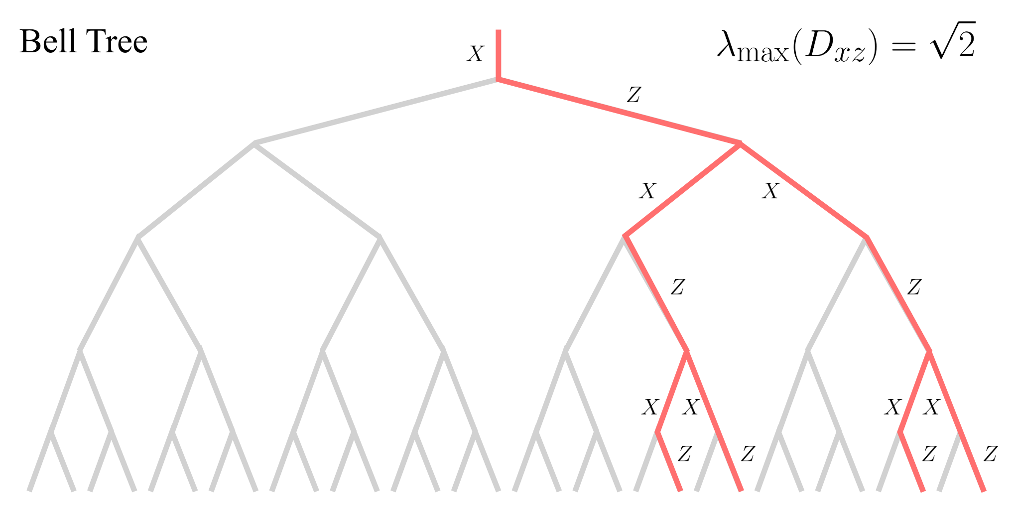
Figure 4: A logical subtree of the Bell Tree: This figure illustrates the $X$ logical subtree associated with the Bell tree, defined in Fig. 2. Recall that this encoder is an anti-standard encoder of a CSS code, namely the binary repetition code. Clearly, in alternate levels, the tree branches into either $1$ or $2$ (i.e., $d_{x}$ or $d_{z}$) children, resulting in an effective branching factor of $\sqrt{1\times 2}$.

III.3 CSS code trees with ‘Anti-standard’ encoders: Bell Tree

Consider a standard encoder for a CSS code, described by an isometry $V$. Now suppose before applying this encoder, we apply the Hadamard gate $H$ on the qubit. The resulting encoder, described by the isometry $VH$ has logical $Z$ operators $Z_{L}\in\langle iI,X\rangle^{\otimes b}$ and the logical $X$ operator $X_{L}\in\langle iI,Z\rangle^{\otimes b}$ with weights $d_{z}={\rm weight}(Z_{L})$ and $d_{x}={\rm weight}(X_{L})$, respectively. We refer to this type of encoder as an “anti-standard” encoder.

We show that in this case Eq.(24) will be modified to

$$|1-2q^{x}_{T}|\leq{\sqrt{2}}\times\sqrt{d_{x}^{\lceil T/2\rceil}\times d_{z}^{\lfloor T/2\rfloor}}\times|1-2p|^{T}\ ,$$ (30)

where for simplicity we have assumed $p=p_{x}=p_{z}$ (see lemma 4). Note that the quantity $d_{x}^{\lceil T/2\rceil}\times d_{z}^{\lfloor T/2\rfloor}$ is the weight of a logical $X$ operator for the encoder $V_{T}$. A similar bound can be obtained for $q^{z}_{T}$ by exchanging $d_{z}$ and $d_{x}$ in the right-hand side of this equation.

We conclude that for $p$ satisfying

$$|1-2p|^{2}\times\sqrt{d_{x}\times d_{z}}<1\ ,$$ (31)

the infinite tree does not transfer any information (note that this lower bound is the geometric mean of the lower bounds in Eq.(25) and Eq.(26) for standard encoders).

As a simple example, consider the repetition code with the isometry $V|c\rangle=|c\rangle^{\otimes b}:c=0,1$, for which $d_{x}=b$ and $d_{z}=1$. From the classical result of Evans et al. (2000) discussed in the introduction, one can show that the infinite tree constructed from this code does not transmit classical information in $|0\rangle,|1\rangle$ basis if, and only if

$$|1-2p_{x}|^{2}\times b<1\ ,$$ (32)

whereas if $p_{z}\neq 0,1$, it does not transfer any information in $X$ (or, $Y$) basis. On the other hand, when we add the Hadamard gate and convert the standard encoder to an anti-standard encoder, no information is transmitted over the infinite tree if

$$|1-2p|^{2}\times\sqrt{b}<1\ ,$$ (33)

where we assume $p_{x}=p_{z}=p$. Therefore, adding the Hadamard gates lowers the noise threshold for transferring classical information encoded in the input $Z$ basis. However, as we will show in the example of the Bell tree, which corresponds to $b=2$, this allows transmission of information encoded in the input $X$ basis and entanglement, even for non-zero $p_{z}>0$. It is worth noting that in the absence of noise, the channel $\mathcal{V}_{2}$ obtained from two layers of the anti-standard encoder is indeed the encoder of the generalized Shor code (see Appendix Sec.D.2 for further discussion).

III.4 Stabilizer Trees with General Encoders

In this section, we establish the exponential decay of information for stabilizer trees constructed from general encoders that are not necessarily standard or anti-standard. Before presenting the most general case in proposition 3, first, we consider encoders that are constructed only from CNOTs and Hadmarad gates. The main relevant property of such encoders is that they have logical $\sigma_{x}$ and logical $\sigma_{z}$ operators $L_{x},L_{z}\in\langle iI,\sigma_{z},\sigma_{x}\rangle^{\otimes b}$, i.e., they do not act as $\sigma_{y}$ operator on any qubits (in this section, for convenience, we use $\sigma_{x},\sigma_{y},$ and $\sigma_{z}$, to denote Pauli $X$, $Y$, and $Z$, respectively). Then, we show that in this case, a modification of the bound in Eq.(III.2) holds.

Proposition 2.

Let $L_{x},L_{z}\in\langle iI,\sigma_{x},\sigma_{z}\rangle^{\otimes b}$ be logical $\sigma_{x}$ and logical $\sigma_{z}$ operators for the encoder $V:\mathbb{C}^{2}\rightarrow(\mathbb{C}^{2})^{\otimes b}$, such that $L_{w}V=V\sigma_{w}\ :w=x,z$. For $v,w\in\{x,z\}$ let $n(v\rightarrow w)$ be the number of qubits on which logical $\sigma_{v}$ acts as $\sigma_{w}$, and

$$b_{\text{max}}=\max\{{\rm weight}(L_{x}),{\rm weight}(L_{z})\}\ ,$$

be the maximum weight of these two logical operators. Let $\lambda_{\text{max}}(D_{xz})$ be the maximum eigenvalue (spectral radius) of the weight transition matrix

$$D_{xz}=\left(\begin{array}[]{cc}n(x\rightarrow x)&n(z\rightarrow x)\\ n(x\rightarrow z)&n(z\rightarrow z)\end{array}\right)\ .$$ (34)

Assume the noise channel $\mathcal{N}$ that defines the tree channel $\mathcal{E}_{T}$ in Eq.(9) is $\mathcal{N}=\mathcal{N}_{x}\circ\mathcal{N}_{z}$, where $\mathcal{N}_{x}$ and $\mathcal{N}_{z}$ are, respectively, the bit-flip and phase-flip channels with probability $p_{x}=p_{z}=p$. If

$$(1-2p)^{2}\times\min\{\lambda_{\text{max}}(D_{xz}),b_{\text{max}}\}<1\ ,$$ (35)

then in the limit $T\rightarrow\infty$, the output of channel $\mathcal{E}_{T}$ becomes independent of the input. More precisely, for any single-qubit density operator $\rho$, it holds that

$$\big{\|}\mathcal{E}_{T}(\rho)-\mathcal{E}_{T}(\frac{I}{2})\big{\|}_{1}\leq{2\sqrt{2}}\times\sqrt{g_{xz}(T)}\times|1-2p|^{T}\ .$$ (36)

Here,

$$g_{xz}(T)=\max_{w\in\{x,z\}}(1,1)D^{T}_{xz}e_{w}\leq b^{T}_{\text{max}}\ ,$$ (37)

is an upper bound on the weights of logical $\sigma_{x}$ and $\sigma_{z}$ operators at level $T$, where $e_{x}=(1,\ 0)^{\rm T}$, $e_{z}=(0,\ 1)^{\rm T}$.

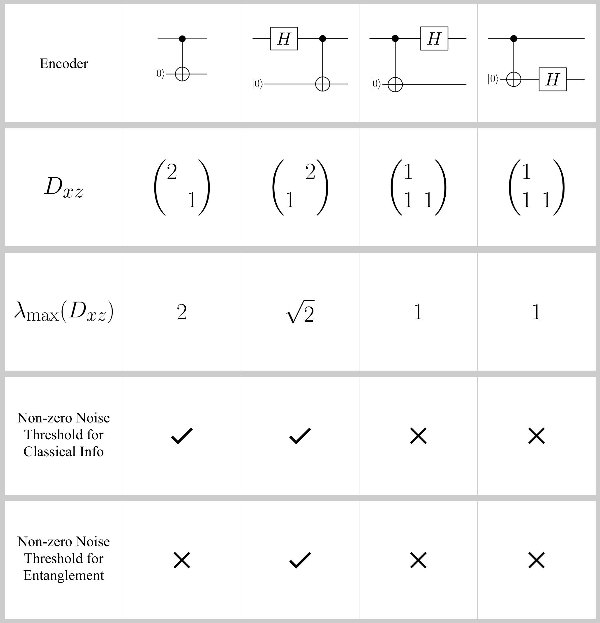
Figure 5: The encoder of the binary repetition code and 3 of its variations obtained by adding a single Hadamard gate to its inputs/outputs. In every circuit, the top qubit is the input data qubit and the bottom qubit is the ancilla initialized in state $\ket{0}$. In addition to these 3 variations, there is a $4^{\rm th}$ variation in which the Hadamard acts on the ancilla before applying the CNOT gate. However, in that case the encoder acts trivially on the input state. For each of these encoders, we indicate their weight transition matrix $D_{xz}$ defined in Eq.(34) and its largest eigenvalue $\lambda_{\text{max}}(D_{xz})$. Furthermore, we indicate whether there exists a non-zero noise threshold below which the tree transmits classical information and/or entanglement to any depth. Eq.(35) puts an upper bound on the noise threshold for classical information in terms of $\lambda_{\text{max}}(D_{xz})$. In particular, for $\lambda_{\text{max}}(D_{xz})=1$ information does not propagate over the infinite tree; this is the case for the $3^{\rm rd}$ and $4^{\rm th}$ encoders. The second column, which is the encoder of the Bell tree in Fig.2 yields a non-zero noise threshold for the propagation of classical information and entanglement on an infinite tree. It is worth noting that the transition matrix $D_{xz}$ is not unique. For instance, for the third encoder one can choose $Z_{L}=XI$ or $Z_{L}=IZ$. With $X_{L}=ZX$, the former choice yields $\lambda_{\rm max}(D_{xz})=(1+\sqrt{5})/2$, whereas for the latter $\lambda_{\rm max}(D_{xz})=1$; we pick the lesser value for the tighter upperbound.

Note that the maximum eigenvalue of $D_{xz}$ is

$$\lambda_{\text{max}}(D_{xz})=n_{\text{avg}}+\sqrt{n_{\text{dif}}^{2}+n_{\text{cross}}^{2}}\ ,$$ (38)

where

$$n_{\text{avg}} =\frac{1}{2}\big{[}n(x\rightarrow x)+n(z\rightarrow z)\big{]}$$ (39a)

$$n_{\text{dif}} =\frac{1}{2}\big{[}n(x\rightarrow x)-n(z\rightarrow z)\big{]}$$ (39b)

$$n_{\text{cross}} =\sqrt{n(x\rightarrow z)\times n(z\rightarrow x)}\ .$$ (39c)

Roughly speaking, this quantity determines the maximum rate of growth of the logical subtrees in the regime $T\rightarrow\infty$ (see Fig.3 and Fig.4). To obtain the strongest bound on the decay of information, one should consider the logical $X$ and $Z$ operators for which $\lambda_{\text{max}}(D_{xz})$ is minimized.

It is worth considering the two special cases of standard and anti-standard encoders of CSS codes. For standard encoders, there exist logical operators with

$$n(z\rightarrow z)=d_{z}\ ,\ \ \ \ n(z\rightarrow x)=0$$

and

$$n(x\rightarrow x)=d_{x}\ ,\ \ \ \ n(x\rightarrow z)=0\ ,$$

which implies

$$\lambda_{\text{max}}(D_{xz})=\frac{1}{2}\big{(}d_{x}+d_{z}\big{)}+\frac{1}{2}|d_{x}-d_{z}|=\max\{d_{x},d_{z}\}\ .$$ (40)

Next, suppose we add a Hadamard to this encoder to obtain an anti-standard encoder with

$$n(z\rightarrow z)=0\ ,\ \ \ \ n(z\rightarrow x)=d_{x}$$

and

$$n(x\rightarrow x)=0\ ,\ \ \ \ n(x\rightarrow z)=d_{z}\ ,$$

which implies

$$\lambda_{\text{max}}(D_{xz})=\sqrt{d_{x}\times d_{z}}\ .$$ (41)

Therefore, the bound in Eq.(36) generalizes the special bounds we have previously seen in the case of standard and anti-standard encoders.

Finally, we consider the most general stabilizer encoder which can be an arbitrary Clifford unitary. In this case, the logical $\sigma_{x}$ and $\sigma_{z}$ operators contain $\sigma_{x}$, $\sigma_{y}$, and $\sigma_{z}$. Then, in this situation, it is more natural to assume a noise model where $X$, $Y$, $Z$ errors happen independently, each with probability $p_{x}=p_{y}=p_{z}=p\leq 1/2$. This corresponds to the depolarizing channel

$$\mathcal{M}_{\epsilon}(\rho)=\mathcal{N}_{x}\circ\mathcal{N}_{y}\circ\mathcal{N}_{z}(\rho)=(1-\epsilon)\rho+\epsilon\frac{I}{2}\ ,$$ (42)

where $\epsilon=4p(1-p)$, and $\mathcal{N}_{w}(\rho)=p\sigma_{w}\rho\sigma_{w}+(1-p)\sigma_{w}$ for $w=x,y,z$.

Proposition 3.

Let $L_{x},L_{y},L_{z}\in\langle iI,\sigma_{x},\sigma_{y},\sigma_{z}\rangle^{\otimes b}$ be logical $\sigma_{x}$, $\sigma_{y}$, and $\sigma_{z}$ operators for the encoder $V:\mathbb{C}^{2}\rightarrow(\mathbb{C}^{2})^{\otimes b}$, such that $L_{w}V=V\sigma_{w}\ :w=x,y,z$. Let $n(v\rightarrow w)$ be the number of qubits on which logical $\sigma_{v}$ acts as $\sigma_{w}$ and consider the corresponding $3\times 3$ matrix

$$D_{xyz}=\left(\begin{array}[]{ccc}n(x\rightarrow x)&n(y\rightarrow x)&n(z\rightarrow x)\\ n(x\rightarrow y)&n(y\rightarrow y)&n(z\rightarrow y)\\ n(x\rightarrow z)&n(y\rightarrow z)&n(z\rightarrow z)\end{array}\right)\ .$$ (43)

Let $\lambda_{\text{max}}(D_{xyz})$ be the spectral radius of $D_{xyz}$, i.e., the largest absolute value of the eigenvalues of $D_{xyz}$, and

$$b_{\text{max}}=\max\{{\rm weight}(L_{x}),{\rm weight}(L_{y}),{\rm weight}(L_{z})\}\ ,$$

be the maximum weight of these logical operators. Assume the noise channel $\mathcal{N}$ that defines the tree channel $\mathcal{E}_{T}$ in Eq.(9) is the depolarizing channel $\mathcal{M}_{\epsilon}$ in Eq.(42). If

$$(1-\epsilon)\times\min\{\lambda_{\text{max}}(D_{xyz}),b_{\text{max}}\}<1\ ,$$ (44)

then in the limit $T\rightarrow\infty$, the output of channel $\mathcal{E}_{T}$ becomes independent of the input. More precisely, for any single-qubit density operator $\rho$, it holds that

$$\big{\|}\mathcal{E}_{T}(\rho)-\mathcal{E}_{T}(\frac{I}{2})\big{\|}_{1}\leq{2\sqrt{2}}\times\sqrt{g_{xyz}(T)\times(1-\epsilon)^{T}}\ .$$ (45)

Here,

$$g_{xyz}(T)=\max_{w\in\{x,y,z\}}\begin{pmatrix}1&1&1\end{pmatrix}D^{T}_{xyz}e_{w}\leq b_{\text{max}}^{T}\ ,$$ (46)

is an upper bound on the weights of logical operators in level $T$, where $e_{x}=(1,0,0)^{\rm T}$, and $e_{y}$ and $e_{z}$, are defined in a similar fashion.

To prove this result, we first show the following lemma, which is a generalization of proposition 1, and is of independent interest. Here, $\mathcal{D}_{w}$ is the single-qubit channel that fully dephases the input qubit in the eigenbasis of $\sigma_{w}$, i.e., $\mathcal{D}_{w}(\rho)=(\rho+\sigma_{w}\rho\sigma_{w})/2$.

Lemma 4.

Let ${L}_{w}[T]\in\langle iI,\sigma_{x},\sigma_{y},\sigma_{z}\rangle^{\otimes b^{T}}$ be a logical $\sigma_{w}$ operator, such that ${L}_{w}[T]V_{T}=V_{T}\sigma_{w}$. Let $\mathcal{N}$ be the noise channel that defines the tree channel $\mathcal{E}_{T}$ in Eq.(9). Then,

$$\big{\|}\mathcal{E}_{T}-\mathcal{E}_{T}\circ\mathcal{D}_{w}\big{\|}^{2}_{\diamond}\leq 2\times r(T)\times{\rm weight}({L}_{w}[T])\ ,$$ (47)

where

• $w=x,y,z$ and $r(T)=(1-\epsilon)^{T}$, provided that $\mathcal{N}$ is the depolarizing channel $\mathcal{M}_{\epsilon}$ in Eq.(42).

• $w=x,z$, and $r(T)=(1-2p)^{2T}$, provided that $\mathcal{N}=\mathcal{N}_{z}\circ\mathcal{N}_{x}$, with the probability of bit-flip and phase-flip errors $p_{x}=p_{z}=p$, and provided that there exists a sequence of operators ${L}_{w}[0]\rightarrow L_{w}[1]\rightarrow\cdots\rightarrow L_{w}[T]$ such that $L_{w}[0]=\sigma_{w}$, $L_{w}[t]\in\langle iI,\sigma_{x},\sigma_{z}\rangle^{\otimes b^{t}}$, and ${L}_{w}[t+1]V^{\otimes b^{t}}=V^{\otimes b^{t}}{L}_{w}[t]$ for all $t\geq 0$.

In particular, in the first case of this lemma, if there exists a sequence of logical operators ${L}_{w}[T]$ such that

$$\lim_{T\rightarrow\infty}(1-\epsilon)^{T}\times{\rm weight}({L}_{w}[T])=0\ ,$$ (48)

then the infinite tree is entanglement-breaking and might only transfer classical information encoded in the eigenbasis of $\sigma_{w}$.

III.5 Proof of Proposition 1

First, recall that the effect of noise inside the tree is equivalent to correlated Pauli noise on the leaves. That is

$$\mathcal{E}_{T}=\mathcal{F}_{T}\circ\mathcal{V}_{T}\ ,$$ (49)

where $\mathcal{V}_{T}$ defined in Eq.(7) is the ideal encoder of the concatenated code associated with the tree, and $\mathcal{F}_{T}$ are correlated Pauli errors on the leaves. In the following, we prove the proposition for the special case of $p_{x}=0$, i.e., when there are no $X$ errors. Clearly, in the presence of $X$ errors, due to the contractivity of the diamond norm under data processing, the upper bound remains valid. Then, for standard encoders, $\mathcal{F}_{T}$ can be thought of as a channel that randomly applies Pauli $Z$ operators on some qubits. To express this we use the following notation: for any bit string $\textbf{z}=z_{1}\cdots z_{n}\in\{0,1\}^{n}$ define

$$\textbf{Z}^{\bf{z}}:=Z^{z_{1}}\otimes\cdots\otimes Z^{z_{n}}\ ,$$ (50)

which means a Pauli $Z$ is applied on those qubits where $\bf{z}$ takes value 1. Then, for standard encoders, $\mathcal{F}_{T}$ can be written as

$$\mathcal{F}_{T}(\cdot)=\sum_{\textbf{z}\in\{0,1\}^{b^{T}}}f_{T}(\textbf{z})\ \textbf{Z}^{\textbf{z}}(\cdot)\textbf{Z}^{\textbf{z}}\ ,$$ (51)

where $f_{T}$ is a probability distribution over $\{0,1\}^{b^{T}}$. It is worth emphasizing that because the output of $\mathcal{V}_{T}$ is restricted to a 2D code subspace, the channel $\mathcal{F}_{T}$, and hence the probability distribution $f_{T}$, are not uniquely defined (as we further explain below, this is related to the freedom of choosing logical operators for a code).

The goal is to bound $\big{\|}\mathcal{E}_{T}-\mathcal{E}_{T}\circ\mathcal{D}_{z}\big{\|}_{\diamond}=\frac{1}{2}\big{\|}\mathcal{E}_{T}-\mathcal{E}_{T}\circ\mathcal{Z}\big{\|}_{\diamond}$, where $\mathcal{Z}(\cdot)=Z(\cdot)Z$ is the channel that applies Pauli $Z$ on the input qubit. We note that

$$\mathcal{E}_{T}\circ\mathcal{Z}=\mathcal{F}_{T}\circ\mathcal{V}_{T}\circ\mathcal{Z}=\mathcal{F}_{T}\circ\mathcal{Z}_{L}[T]\circ\mathcal{V}_{T}\ ,$$ (52)

where $\mathcal{Z}_{L}[T]$ is the quantum channel corresponding to a logical $Z$ operator at the leaves. More precisely,

$$\mathcal{Z}_{L}[T](\cdot)=\textbf{Z}^{\textbf{z}_{L}[T]}(\cdot)\textbf{Z}^{\textbf{z}_{L}[T]}\ ,$$ (53)

where $\textbf{z}_{L}[T]\in\{0,1\}^{b^{T}}$ is a bit string of length $b^{T}$ satisfying

$$\eta V_{T}Z=\textbf{Z}^{\textbf{z}_{L}[T]}V_{T}\ ,$$ (54)

where $\eta\in\{\pm 1,\pm i\}$ is a global phase. In other words, $\textbf{z}_{L}[T]$ determines on which qubits the logical operator $\eta\textbf{Z}^{\textbf{z}_{L}[T]}$ acts as the identity operator and on which qubits it acts as Pauli $Z$.

We conclude that

$$\big{\|}\mathcal{E}_{T}-\mathcal{E}_{T}\circ\mathcal{Z}\big{\|}_{\diamond} =\big{\|}\mathcal{F}_{T}\circ\mathcal{V}_{T}-\mathcal{F}_{T}\circ\mathcal{Z}_{L}[T]\circ\mathcal{V}_{T}\big{\|}_{\diamond}$$

$$\leq\big{\|}\mathcal{F}_{T}-\mathcal{F}_{T}\circ\mathcal{Z}_{L}[T]\big{\|}_{\diamond}\ ,$$ (55)

where the inequality follows from the contractivity of the diamond norm.

Next, using Eq.(51) we note that

$$\mathcal{F}_{T}\circ\mathcal{Z}_{L}[T](\cdot)=\sum_{\textbf{z}\in\{0,1\}^{N}}f_{T}(\textbf{z}+\textbf{z}_{L}[T])\ \textbf{Z}^{\textbf{z}}(\cdot)\textbf{Z}^{\textbf{z}}\ ,$$ (56)

where $\textbf{z}+\textbf{z}_{L}[T]$ is the bitwise addition of z and $\textbf{z}_{L}[T]$ mod 2. Then, using properties of the diamond norm, this implies

$$\big{\|}\mathcal{F}_{T}-\mathcal{Z}_{L}[T]\circ\mathcal{F}_{T}\big{\|}_{\diamond}$$

$$=\big{\|}\sum_{\textbf{z}\in\{0,1\}^{N}}\big{[}f_{T}(\textbf{z})-f_{T}(\textbf{z}+\textbf{z}_{L}[T])\big{]}\ \textbf{Z}^{\textbf{z}}(\cdot)\textbf{Z}^{\textbf{z}}\big{\|}_{\diamond}$$

$$=\sum_{\textbf{z}\in\{0,1\}^{N}}\big{|}f_{T}(\textbf{z}+\textbf{z}_{L}[T])-f_{T}(\textbf{z})\big{|}\ ,$$ (57)

where the last step is explained in Appendix B.1 (this can be seen, e.g., using the triangle inequality for the diamond norm, which implies the left-hand side is less than or equal to the right-hand, together with the fact that the equality is achieved when all the qubits are prepared in state $|+\rangle$).

Putting everything together we conclude that

$$\big{\|}\mathcal{E}_{T}-\mathcal{E}_{T}\circ\mathcal{D}_{z}\big{\|}_{\diamond} \leq\frac{1}{2}\big{\|}\mathcal{F}_{T}-\mathcal{Z}_{L}[T]\circ\mathcal{F}_{T}\big{\|}_{\diamond}$$ (58)

$$=\frac{1}{2}\sum_{\textbf{z}\in\{0,1\}^{N}}\big{|}f_{T}(\textbf{z}+\textbf{z}_{L}[T])-f_{T}(\textbf{z})\big{|}\ .$$

The second line is the total variation distance between the distribution $f_{T}$ and the distribution obtained from $f_{T}$ by flipping all those bits where $\textbf{z}_{L}[T]$ is 1. As mentioned before, neither $f_{T}$ nor $\textbf{z}_{L}[T]$ are unique. One is free to choose any distribution $f_{T}$ such that the corresponding channel $\mathcal{F}_{T}$ defined in Eq.(51) satisfies Eq.(49). Similarly, one can choose any logical operator $\textbf{Z}^{\textbf{z}_{L}[T]}$ that satisfies Eq.(54). But, clearly, given the structure of the tree, it is natural to choose the logical operator $\textbf{Z}^{\textbf{z}_{L}[T]}$ and the distribution $f_{T}$ in a way that is defined by the recursive application of the same rule on all nodes of the tree.

In particular, let $\eta\textbf{Z}^{\textbf{z}_{L}[1]}$ be a logical $Z$ operator for the original code that is applied at each node of the tree, i.e.,

$$VZ=\eta\textbf{Z}^{\textbf{z}_{L}[1]}V\ ,$$ (59)

where $\eta\in\{\pm 1,\pm i\}$ is a global phase. Then, we can define a chain of bit strings

$$1\rightarrow\textbf{z}_{L}[1]\rightarrow\cdots\rightarrow\textbf{z}_{L}[T]\ ,$$ (60)

where $\textbf{z}_{L}[t+1]\in\{0,1\}^{b^{t+1}}$ is obtained from $\textbf{z}_{L}[t]\in\{0,1\}^{b^{t}}$ by replacing any 0 in $\textbf{z}_{L}[t]$ with $0^{b}$ and any 1 with $\textbf{z}_{L}[1]$.

Then, for all $t$ it holds that

$$V_{t}Z=\eta\textbf{Z}^{\mathbf{z}_{L}[t]}V_{t}\ ,$$ (61)

for some $\eta\in\{\pm 1,\pm i\}$. For each level $t\leq T$, consider the nodes where $\textbf{z}_{L}[t]$ takes value 1. The set of such nodes defines a logical subtree. For instance, in the example in Figure 3, this corresponds to the highlighted 3-ary subtree.

Next, we discuss the distribution $f_{T}$. Recall that this distribution should be chosen such that Eq.(49) is satisfied by $\mathcal{F}_{T}$. We choose to define this distribution recursively in a way that is consistent with the above chain of logical operators. In particular, we define $f_{T}$ via the recursive equation

$$\mathcal{F}_{t+1}(\cdot) =\sum_{\textbf{z}\in\{0,1\}^{b^{t+1}}}f_{t+1}(\textbf{z})\ \textbf{Z}^{\textbf{z}}(\cdot)\textbf{Z}^{\textbf{z}}\ ,$$ (62)

$$=\mathcal{N}_{z}^{\otimes b^{t+1}}\circ\sum_{\textbf{w}\in\{0,1\}^{b^{t}}}f_{t}(\textbf{w})\ \textbf{Z}_{L}^{\textbf{w}}(\cdot)\textbf{Z}_{L}^{\textbf{w}}\ ,$$

where $f_{0}(0)=1$ and $f_{0}(1)=0$, and for any $\textbf{w}=w_{1}\cdots w_{t}$ $\textbf{Z}^{\textbf{w}}_{L}$ denotes

$$\textbf{Z}_{L}^{\textbf{w}} =\textbf{Z}^{w_{1}\times\textbf{z}_{L}[1]}\otimes\cdots\cdots\otimes\textbf{Z}^{w_{t}\times\textbf{z}_{L}[1]}=\textbf{Z}^{\textbf{w}^{\prime}}\ ,$$ (63)

where ${\textbf{w}^{\prime}}$ is the bit string of length $b^{t+1}$ obtained from w by replacing all $0$ and $1$ in w by $0^{b}$ and $\textbf{z}_{L}[1]$, respectively. This definition implies

$$\textbf{Z}^{\textbf{w}^{\prime}}V^{\otimes b^{t}}=\textbf{Z}_{L}^{\textbf{w}}V^{\otimes b^{t}}=V^{\otimes b^{t}}\textbf{Z}^{\textbf{w}}\ .$$ (64)

Composing both sides of Eq.(62) from the right-hand side with $\mathcal{V}^{\otimes b^{t}}$ and applying Eq.(64) implies

$$\mathcal{F}_{t+1}\circ\mathcal{V}^{\otimes b^{t}}=\mathcal{N}_{z}^{\otimes b^{t+1}}\circ\mathcal{V}^{\otimes b^{t}}\circ\mathcal{F}_{t}\ ,$$ (65)

for all $t$, which in turn implies

$$\mathcal{F}_{T}\circ\mathcal{V}_{T}=\prod_{j=0}^{T-1}\mathcal{N}_{z}^{\otimes b^{j+1}}\circ\mathcal{V}^{\otimes b^{j}}=\mathcal{E}_{T}\ ,$$ (66)

as required.

Note that Eq.(62) has a simple interpretation: to sample a bit string $\textbf{z}\in\{0,1\}^{b^{t+1}}$ according to the distribution $f_{t+1}$, one first samples a bit string $\textbf{w}\in\{0,1\}^{b^{t}}$ according to the distribution $f_{t}$, then replace any 0 in w with $0^{b}$ and any 1 in w with $\textbf{z}_{L}[1]$, and finally flips each bit randomly and independently with probability $p_{z}$. This definition has an important implication for the distribution $f_{T}$: the bits inside the logical subtree defined by the sequence of logical operators in Eq.(60) are uncorrelated with the bits outside this subtree. Furthermore, $\textbf{z}_{L}[T]$ only acts inside this subtree. It follows that discarding the bits outside the logical subtree does not change the total variation in the second line of Eq.(58). That is

$$\frac{1}{2}\sum_{\textbf{z}\in\{0,1\}^{b^{T}}}\big{|}f_{T}(\textbf{z}+\textbf{z}_{L}[T])-f_{T}(\textbf{z})\big{|}$$

$$=\frac{1}{2}\sum_{\textbf{w}\in\{0,1\}^{b_{z}^{T}}}\big{|}g_{T}(\textbf{w}+\textbf{1}^{b_{z}^{T}})-g_{T}(\textbf{w})\big{|}\ ,$$ (67)

where $g_{T}$ is the marginal distribution associated to the $b_{z}^{T}$ bits on which $\textbf{z}_{L}[T]$ is 1, and $\textbf{1}^{b_{z}^{T}}$ is a bit string with $b_{z}^{T}$ 1’s. The distribution $g_{T}$ has a simple interpretation in terms of the classical broadcasting problem discussed in the introduction: consider the distribution associated with the leaves of a full $b_{z}$-ary tree with depth $T$, where at each edge the bit is flipped with probability $p_{z}$. Then, for the input 0 at the root of the tree, the probability that leaves are in the bit string $\textbf{w}\in\{0,1\}^{b_{z}^{T}}$ is $g_{T}(\textbf{w})$ and for the input 1, this probability is $g_{T}(\textbf{w}+\textbf{1}^{b_{z}^{T}})$.

Therefore, we can apply the results on classical broadcasting on trees and, in particular, the results of Evans et al. (2000) to bound the total variation distance in Eq.(67). In particular, as we explain in the Appendix A, applying Theorem 1.3 of Evans et al. (2000) we find

$$\frac{1}{2}\sum_{\textbf{w}\in\{0,1\}^{b_{z}^{T}}}\big{|}g_{T}(\textbf{w}+\textbf{1}^{b_{z}^{T}})-g_{T}(\textbf{w})\big{|}\leq{\sqrt{2}}\Big{[}\sqrt{b_{z}}\times|1-2p_{z}|\Big{]}^{T}\ .$$ (68)

Combining this with Eq.(58) and Eq.(67), we arrive at

$$\big{\|}\mathcal{E}_{T}-\mathcal{E}_{T}\circ\mathcal{D}_{z}\big{\|}_{\diamond}\leq{\sqrt{2}}\Big{[}\sqrt{b_{z}}\times|1-2p_{z}|\Big{]}^{T}\ ,$$

which completes the proof of proposition 1.

III.6 Proofs of propositions 2 and 3 and lemma 4

Here, we explain how proposition 1 can be generalized to propositions 2 and 3 and lemma 4 that apply to general stabilizer codes with general encoders. We mainly focus on proving proposition 3 and lemma 4. Proof of proposition 2 follows in a similar fashion.

First, note that the idea of a logical subtree can be straightforwardly generalized to the trees in Proposition 2 or 3. In particular, using the same approach that we used to define the sequence in Eq.(60), for $w\in\{x,y,z\}$ we define the sequence of logical operators

$${L}_{w}[0]\rightarrow L_{w}[1]\rightarrow\cdots\rightarrow L_{w}[T]\ ,$$ (69)

such that

$${L}_{w}[t+1]V^{\otimes b^{t}}=V^{\otimes b^{t}}{L}_{w}[t]\ ,$$ (70)

where

$${L}_{w}[t]\in\langle iI,\sigma_{x},\sigma_{y},\sigma_{z}\rangle^{\otimes b^{t}}\ ,$$

and, in particular, ${L}_{w}[0]=\sigma_{w}$ is a Pauli operator. It is also worth noting that given any operator ${L}_{w}[T]\in\langle iI,\sigma_{x},\sigma_{y},\sigma_{z}\rangle^{\otimes b^{T}}$ satisfying ${L}_{w}[T]V_{T}=V_{T}\sigma_{w}$ for

$$V_{T}=\prod_{j=0}^{T-1}V^{\otimes{b}^{j}}\ ,$$

one can find a sequence of logical operators in the form of Eq.(69) satisfying Eq.(70).

Given this sequence, we can extract a logical subtree where at each level $t$, the nodes of this subtree correspond to those qubits on which operator $L_{w}[t]$ acts non-trivially, i.e., acts as one of the Pauli operators. Furthermore, this definition also associates one of the “types” $x,y$, or $z$ to each node in the logical subtree: namely, the type of each node at level $t$ is determined by the Pauli operator in $L_{w}[t]$ that acts on the qubit in that node. Similarly, we can associate a type $x,y$, or $z$ to each edge in this subtree: an edge connecting a node at level $t$ to a node at level $t+1$, has the same type as the node at level $t$, i.e., the parent node.

Now consider the noisy tree channel $\mathcal{E}_{T}$. Each edge in this tree corresponds to a single-qubit channel $\mathcal{N}$, where $\mathcal{N}=\mathcal{N}_{x}\circ\mathcal{N}_{z}$ in proposition 2, and $\mathcal{N}=\mathcal{N}_{x}\circ\mathcal{N}_{y}\circ\mathcal{N}_{z}$ in proposition 3. In the proof of proposition 1, we began by ignoring the bit-flip noise channels $\mathcal{N}_{x}$ on all edges. Similarly, for the proof of proposition 2 and 3 we selectively discard the noises that are not consistent with an edge’s type. In proposition 2 this means discarding one of the channels $\mathcal{N}_{x}$ or $\mathcal{N}_{z}$ in $\mathcal{N}=\mathcal{N}_{x}\circ\mathcal{N}_{z}$, and in proposition 3 we discard $\mathcal{N}_{x}\circ\mathcal{N}_{y}$ from $\mathcal{N}_{x}\circ\mathcal{N}_{y}\circ\mathcal{N}_{z}$, if the edge type is $z$, and similarly for $x$ and $y$. By doing so, we ensure that for each qubit in the logical subtree, the Pauli type associated with the logical operator acting on the qubit is the same as the type of Pauli noise on the qubit. Note that here we again rely on the monotonicity of the diamond norm distance under data processing.

Now recall that we had set all the flip probabilities in channels $\mathcal{N}_{x}$, $\mathcal{N}_{y}$, and $\mathcal{N}_{z}$ to be $p$, which in the case of proposition 3 is $p=(1-\sqrt{1-\epsilon})/2$. Thus, at this juncture, we may presume that we have a logical subtree of just one type of operator, say $Z$, and all its edges have only phase-flip errors with probability $p$. In other words, the logical subtree we obtain after discarding ‘inconsistent’ noise differs from the tree obtained in the proof of proposition 1 by a reference frame change on each edge.

Thus, we can apply the same proof technique as discussed for proposition 1, but for the logical subtree obtained for general encoders. The only important difference between the two cases is that the logical subtree will not correspond to a full $b_{z}$-ary tree, as in Eq.(68). However, fortunately, as we explain in Appendix A, Theorem 1.3’ of Evans et al. (2000) allows us to upper bound the total variation distance in Eq.(68), for arbitrary trees. In particular, for the logical subtree obtained from the sequence in Eq.(69), the same bound in Eq.(68) remains valid, provided that we replace $\sqrt{b_{z}^{T}}$ in the right-hand side of Eq.(68) with the more general expression $\sqrt{{\rm weight}(L_{w}[T])}$. Then, we conclude that

$$\big{\|}\mathcal{E}_{T}-\mathcal{E}_{T}\circ\mathcal{D}_{w}\big{\|}^{2}_{\diamond} \leq 2\times{\rm weight}(L_{w}[T])\times|1-2p|^{2T}\ ,$$

$$=2\times{\rm weight}(L_{w}[T])\times(1-\epsilon)^{T}\ ,$$

which proves the first part of lemma 4. The second part of the lemma follows similarly.

Next, to prove proposition 3 we note that

$$\big{\|}\mathcal{E}_{T}(\rho)-\mathcal{E}_{T}(\frac{I}{2})\big{\|}_{1}=\big{\|}\mathcal{E}_{T}(\rho)-\mathcal{E}_{T}\circ\mathcal{D}_{x}\circ\mathcal{D}_{z}(\rho)\big{\|}_{1}$$ (71)

$$\leq\big{\|}\mathcal{E}_{T}-\mathcal{E}_{T}\circ\mathcal{D}_{x}\circ\mathcal{D}_{z}\big{\|}_{\diamond}$$

$$\leq\big{\|}\mathcal{E}_{T}-\mathcal{E}_{T}\circ\mathcal{D}_{x}\big{\|}_{\diamond}+\big{\|}\mathcal{E}_{T}\circ\mathcal{D}_{x}-\mathcal{E}_{T}\circ\mathcal{D}_{x}\circ\mathcal{D}_{z}\big{\|}_{\diamond}$$

$$\leq\big{\|}\mathcal{E}_{T}-\mathcal{E}_{T}\circ\mathcal{D}_{x}\big{\|}_{\diamond}+\big{\|}\mathcal{E}_{T}-\mathcal{E}_{T}\circ\mathcal{D}_{z}\big{\|}_{\diamond}$$

$$\leq\sqrt{2(1-\epsilon)^{T}}\times\Big{(}\sqrt{{\rm weight}(L_{x}[T])}+\sqrt{{\rm weight}(L_{z}[T])}\Big{)}\ ,$$

where the second line follows immediately from the definition of the diamond norm, the third line follows from the triangle inequality, the fourth line follows from the contractivity of the diamond norm and the last line follows from lemma 4, which is proven above.

Now to prove proposition 3, suppose the sequence of logical operators in Eq.(69) is obtained by concatenating the same logical operators $L_{w}[1]\in\langle i\sigma_{0},\sigma_{x},\sigma_{y},\sigma_{z}\rangle^{\otimes b}$ for $w\in\{0,x,y,z\}$, where $\sigma_{0}=I$ and $L_{0}[1]=\sigma_{0}^{\otimes b}=I^{\otimes b}$ are the identity and logical identity operators, respectively. That is, for

$${L}_{w}[t]=\sigma_{v_{1}}\otimes\cdots\otimes\sigma_{v_{b^{t}}}\ ,$$

with $v_{1},\cdots,v_{b^{t}}\in\{0,x,y,z\}$, we define

$${L}_{w}[t+1]={L}_{v_{1}}[1]\otimes\cdots\otimes{L}_{v_{b^{t}}}[1]\ ,$$

which satisfies Eq.(70).

Next, we determine the number of different Pauli operators in ${L}_{w}[T]$. For a fixed $w\in\{x,y,z\}$, suppose the number of Pauli operators $\sigma_{x},\sigma_{y}$, and $\sigma_{z}$ in the logical operator ${L}_{w}[t]$ are denoted as $n^{x}_{t}$, $n^{y}_{t}$, and $n^{z}_{t}$, respectively. Then, at level $t+1$, we obtain

$$\begin{pmatrix}n^{x}_{t+1}\\ n^{y}_{t+1}\\ n^{z}_{t+1}\end{pmatrix}=\begin{pmatrix}n(x\rightarrow x)&n(y\rightarrow x)&n(z\rightarrow x)\\ n(x\rightarrow y)&n(y\rightarrow y)&n(z\rightarrow y)\\ n(x\rightarrow z)&n(y\rightarrow z)&n(z\rightarrow z)\end{pmatrix}\begin{pmatrix}n^{x}_{t}\\ n^{y}_{t}\\ n^{z}_{t}\end{pmatrix}\ ,$$ (72)

where this $3\times 3$ transition matrix is denoted as $D_{xyz}$. Then,

$${\rm weight}(L_{w}[T]) =n^{x}_{T}+n^{y}_{T}+n^{z}_{T}$$

$$=\begin{pmatrix}1&1&1\end{pmatrix}D^{T}_{xyz}e_{w}\$$

$$\leq g_{xyz}(T)$$

$$\leq b^{T}_{\text{max}}\ .$$

Here, the second line is the sum of the matrix elements of matrix $D^{T}_{xyz}$ in the column associated with $w\in\{x,y,z\}$, the upper bound in the third line corresponds to the maximum between these 3 columns, and the last line follows from the fact that ${\rm weight}(L_{w}[t+1])\leq b_{\text{max}}\times{\rm weight}(L_{w}[t])$. Combining the above bound on ${\rm weight}(L_{w}[T])$ with Eq.(71) proves Eq.(45), i.e.,

$$\big{\|}\mathcal{E}_{T}(\rho)-\mathcal{E}_{T}(\frac{I}{2})\big{\|}_{1}$$ (73)

$$\leq{2\sqrt{2}}\max_{w\in\{x,y,z\}}\sqrt{\begin{pmatrix}1&1&1\end{pmatrix}\Big{[}(1-\epsilon)D_{xyz}\Big{]}^{T}e_{w}}\$$

$$\leq{2\sqrt{2}}\times\big{(}\sqrt{b_{\text{max}}\times(1-\epsilon)}\big{)}^{T}\ .$$

Finally, recall that for any square matrix $A$, $\lim_{n\rightarrow\infty}A^{n}=0$ if, and only if, its spectral radius $\lambda_{\text{max}}(A)<1$. It follows that if $(1-\epsilon)\times\lambda_{\text{max}}(D_{xyz})<1$, or if $(1-\epsilon)\times b_{\text{max}}<1$, then in the limit $T\rightarrow\infty$ the right-hand side of the above bound goes to zero, implying that the output of channel $\mathcal{E}_{T}$ becomes independent of the input. This completes the proof of proposition 3. Proposition 2 can be shown in a similar fashion.

IV Recursive Decoding of Trees with $d\geq 3$ codes

In the previous section, we showed that above certain noise thresholds classical information and entanglement decay exponentially with depth $T$ and vanish in the limit $T\rightarrow\infty$. But, is there any non-zero noise level that allows the propagation of classical information and entanglement over the infinite tree? In this section, we answer in the affirmative by considering a simple recursive local decoding strategy for stabilizer trees with distance $d\geq 3$.

We first explain the idea for general encoders and noise channels and then consider the special case of stabilizer codes with Pauli channels. Consider one layer of the tree channel, the channel $\mathcal{N}^{\otimes b}\circ\mathcal{V}$ that first encodes one input qubit in $b$ qubits and then sends each qubit through the single-qubit noise channel $\mathcal{N}$. Let $\mathcal{R}:\mathcal{L}(({\mathbb{C}^{2}})^{\otimes b})\rightarrow\mathcal{L}(\mathbb{C}^{2})$ be a channel that (approximately) reverses this process, such that the concatenated channel $f[\mathcal{N}]=\mathcal{R}\circ\mathcal{N}^{\otimes b}\circ\mathcal{V}$ is as close as possible to the identity channel (e.g., with respect to the diamond norm, or the entanglement fidelity), where for any single-qubit channel $\mathcal{M}$, we have defined

$$f[\mathcal{M}]\equiv\mathcal{R}\circ\mathcal{M}^{\otimes b}\circ\mathcal{V}\ .$$ (74)

As depicted in Figure 6, by applying this recovery recursively, we find a recovery for the channel corresponding to the entire tree of depth $T$, denoted by ${\mathcal{E}}_{T}=\prod_{j=0}^{T-1}\mathcal{N}^{\otimes b^{j+1}}\circ\mathcal{V}^{\otimes b^{j}}$, or $\widetilde{\mathcal{E}}_{T}={\mathcal{E}}_{T}\circ\mathcal{N}$, if we consider the noise at the input qubit. Namely, the recovery is

$$\mathcal{R}^{\rm loc}_{T}=\prod^{T-1}_{i=0}\mathcal{R}^{\otimes b^{T-i-1}}\ .$$ (75)

As we will see in the following, in general, this is a sub-optimal recovery strategy. However, the advantage of this approach is that implementing the recovery does not require long-range interactions between distant qubits. More precisely, the error corrections are decided locally based on the observed syndromes from only one block with $b$ qubits. Hence, we sometimes refer to this approach as local recovery, as opposed to the optimal recovery that would make a ‘global’ decision based on all observed syndromes together (see Sec.VII). Furthermore, as we discuss below, analyzing the performance of this recovery is relatively easy. We note that the recursive recovery approach has been previously studied in the context of concatenated codes with noiseless encoders Rahn et al. (2002) (in the language of this paper, this corresponds to the tree in which uncorrelated noise channels are applied to the qubits in the leaves, but not inside the tree).

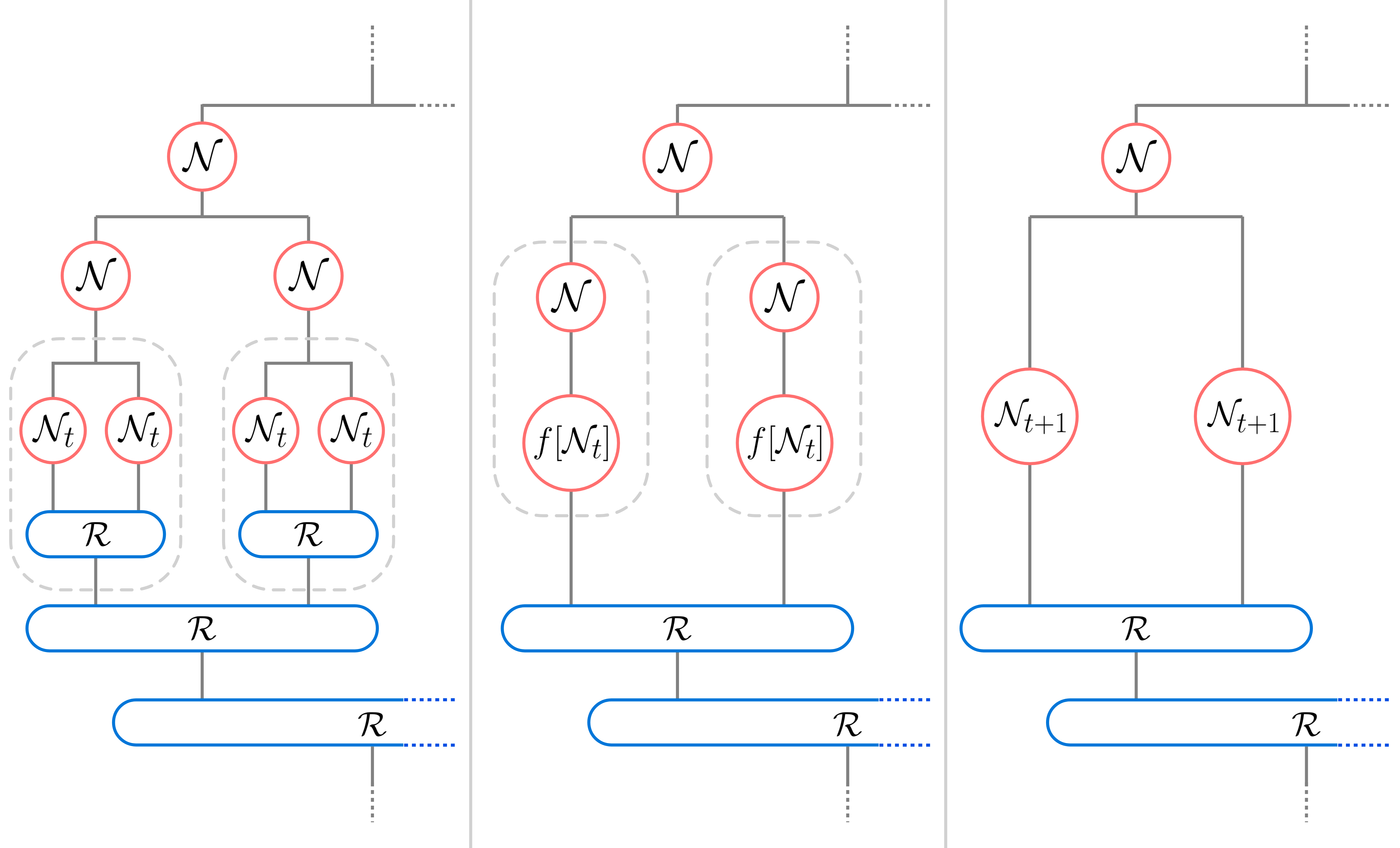
Figure 6: Derivation of the recursive equation 78: After recovery upto level $t$, the effective noise channel is described by the single-qubit noise channel $\mathcal{N}_{t}$ defined in Eq.(76) (see the left image). In the middle image, we consider the single qubit channel obtained after applying recovery to a single block, i.e., $f[\mathcal{N}_{t}]=\mathcal{R}\circ\mathcal{N}_{t}^{\otimes b}\circ\mathcal{V}$ ($b=2$ in this diagram). In the right image, we compose this with the physical noise in the tree, i.e., $\mathcal{N}_{t+1}=f[\mathcal{N}_{t}]\circ\mathcal{N}$. Thus, the effective noise at the next level $t+1$ is denoted by $\mathcal{N}_{t+1}$.

IV.1 Fixed-point equation for infinite tree

For a tree with depth $t$, let $\mathcal{N}_{t}$ be the overall noise after applying the above recovery process to channel $\widetilde{\mathcal{E}}_{t}$, i.e.,

$$\mathcal{N}_{t}=\mathcal{R}^{\rm loc}_{t}\circ\widetilde{\mathcal{E}}_{t}=\mathcal{R}^{\rm loc}_{t}\circ{\mathcal{E}}_{t}\circ\mathcal{N}\ .$$ (76)

As seen in Figure 7, in a tree with depth $t+1$ there are $b$ subtrees each with depth $t$. For each subtree the effective error after error correction is $\mathcal{N}_{t}$. Then, ignoring the single-qubit channel $\mathcal{N}$ at the root of the tree with depth $t+1$, the overall noise is

$$f(\mathcal{N}_{t})=\mathcal{R}\circ\mathcal{N}_{t}^{\otimes b}\circ\mathcal{V}\ .$$ (77)

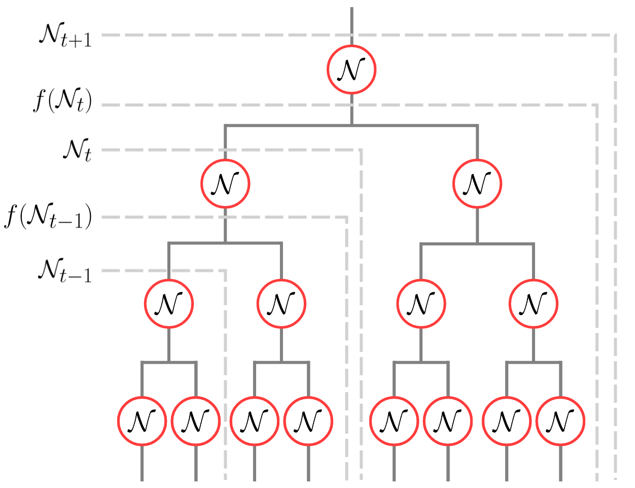
Figure 7: This figure illustrates the steps of recursive decoding of a tree. $\mathcal{N}_{t-1}$ and $\mathcal{N}_{t}$ are single-qubit channels obtained after the local recovery of subtrees of depth $t-1$ and $t$, respectively. $\mathcal{N}_{t}$ can be expressed as a function of $\mathcal{N}_{t-1}$ and $\mathcal{N}$, as summarized in Eq.(78). This way of indexing local recovery levels will be followed in the rest of this paper.

Finally, adding the effect of the single-qubit channel $\mathcal{N}$ at the root, we obtain the overall noise channel

$$\mathcal{N}_{t+1}=f(\mathcal{N}_{t})\circ\mathcal{N}=\mathcal{R}\circ\mathcal{N}^{\otimes b}_{t}\circ\mathcal{V}\circ\mathcal{N}\ .$$ (78)

Fig. 6 illustrates Eq.(78). With the initial condition $\mathcal{N}_{0}=\mathcal{N}$, this recursive equation fully determines $\mathcal{N}_{t}$ for arbitrary $t$. Then, in the limit $t\rightarrow\infty$, we obtain the single-qubit channel

$$\mathcal{N}_{\infty}=\lim_{t\rightarrow\infty}\mathcal{N}_{t}=\lim_{t\rightarrow\infty}\mathcal{R}^{\rm loc}_{t}\circ\widetilde{\mathcal{E}}_{t}\ ,$$ (79)

where we assume that the recovery channel is chosen properly such that this limit exists. This channel satisfies the fixed-point equation

$$\mathcal{N}_{\infty}=f(\mathcal{N}_{\infty})\circ\mathcal{N}=\mathcal{R}\circ\mathcal{N}_{\infty}^{\otimes b}\circ\mathcal{V}\circ\mathcal{N}\ .$$ (80)

Note that the single-qubit channel $\mathcal{N}_{T}$ describes the output of the recursive recovery applied to the channel $\widetilde{\mathcal{E}}_{T}={\mathcal{E}}_{T}\circ\mathcal{N}$, which includes channel $\mathcal{N}$ at the input. On the other hand, if one does not include the single-qubit noise at the input of the tree, then the overall channel is described by $f(\mathcal{N}_{T-1})$, and in the limit $T\rightarrow\infty$, one obtains the channel $f(\mathcal{N}_{\infty})$.

Depending on the strength of the noise in the single-qubit channel $\mathcal{N}$ and the properties of the encoder $\mathcal{V}$, the channel $\mathcal{N}_{\infty}$(or, $f(\mathcal{N}_{\infty})$) might be a channel with constant output which does not transmit any information, i.e., with zero classical capacity, an entanglement-breaking channel with nonzero classical capacity, or a channel that transmits entanglement (and hence even classical information).

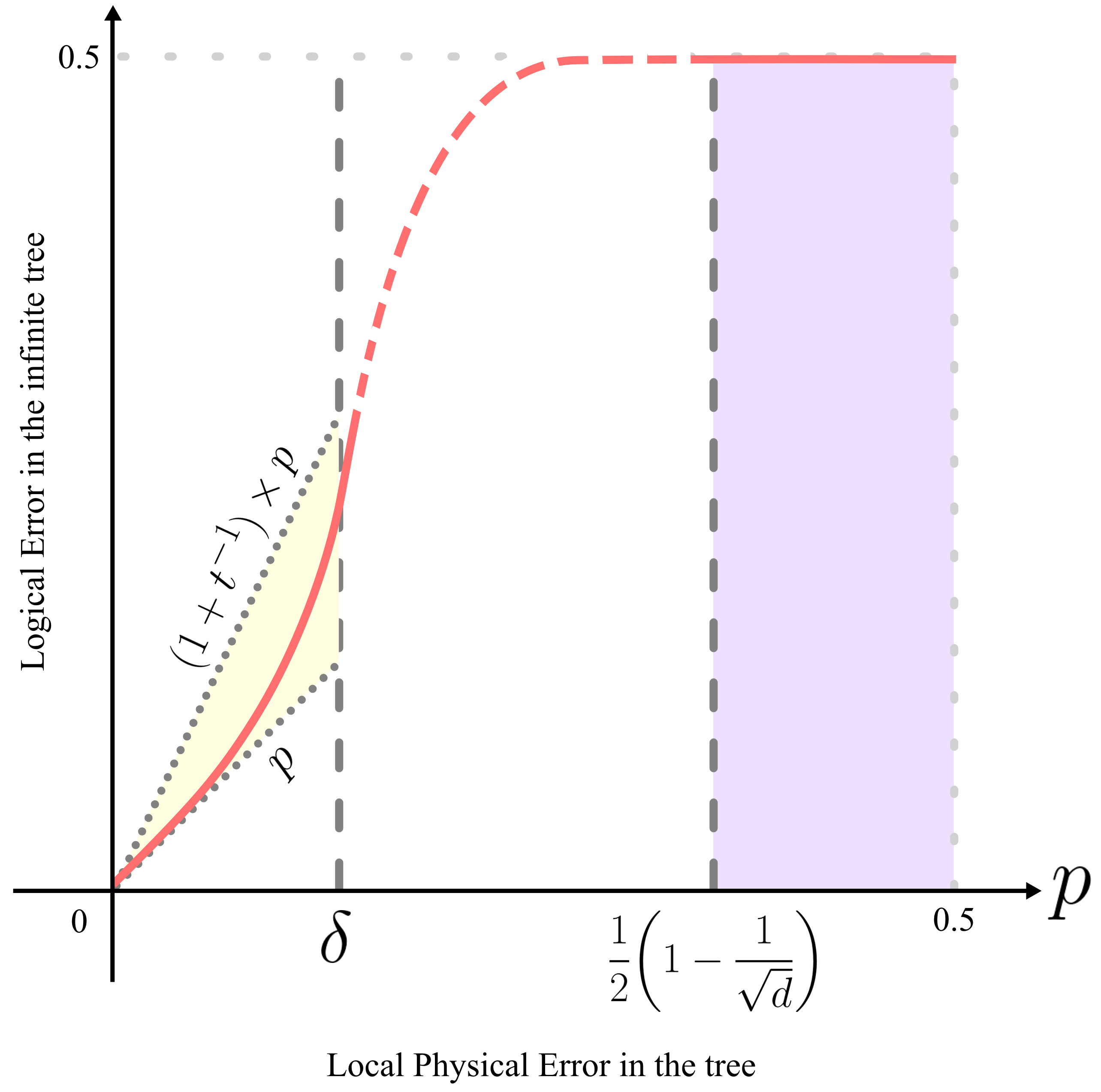
Figure 8: Summary of results for CSS code trees with distance $d\geq 3$ – This plot illustrates the general behavior of the logical $Z$ error $q_{T}^{z}$ in the channel $\widetilde{\mathcal{E}}_{T}=\mathcal{E}_{T}\circ\mathcal{N}$, in the limit $T\rightarrow\infty$ (i.e., the infinite tree with noise on the root) as a function of the physical $Z$ error $p$ on the edges of the tree. Here, $d$ is the code distance, which in particular, means upto $t=\lfloor d-1\rfloor/2$, $Z$ errors can be corrected. We characterize three regions, $p<\delta\equiv\frac{t}{1+t}\big{(}\frac{1}{c(1+t)}\big{)}^{\frac{1}{t}}$ (region I), $p>\frac{1}{2}\big{(}1-\frac{1}{\sqrt{d}}\big{)}$ (region III), and the region in between (region II). From proposition 5 on local recovery analysis, we see that in region I, the logical error is bounded between $p$ and $(1+t^{-1})\times p$, and it is $p+\mathcal{O}(p^{2})$ for $p\ll 1$. From our upperbound on the noise threshold, we see that in region III, the logical error in the infinite tree saturates to $1/2$. The form of the curve in region II remains unknown, but it can be estimated for specific trees using the optimal recovery strategy in Sec VII.

IV.2 Recursive decoding of CSS code trees
(A lower bound on the noise threshold)

In the following, we further study this approach for the case of CSS trees with standard encoders. In Appendix C.4 we explain how these results can be extended to general stabilizer trees.

We consider the recovery channel $\mathcal{R}^{\rm loc}_{T}$ defined in Eq.(75) applied to a CSS code tree $\widetilde{\mathcal{E}}_{T}$ which acts on $X$ and $Z$ errors separately. This ensures,

$$\mathcal{R}^{\rm loc}_{T}\circ\widetilde{\mathcal{E}}_{T}=\mathcal{Q}_{z}\circ\mathcal{Q}_{x}=\mathcal{Q}_{x}\circ\mathcal{Q}_{z}\ ,$$ (81)

where $\mathcal{Q}_{z}=q^{z}_{T}\rho+(1-q^{z}_{T})Z\rho Z$ is a phase flip channel, and $\mathcal{Q}_{x}=q^{x}_{T}\rho+(1-q^{x}_{T})X\rho X$ is a bit flip channel. Since the cases of $Z$ and $X$ errors are similar, we focus on the recovery of $Z$ errors and prove a lower bound on the noise threshold.

Proposition 5.

Consider the tree channel $\widetilde{\mathcal{E}}_{T}=\mathcal{E}_{T}\circ\mathcal{N}$ constructed from a standard encoder of a CSS code, as defined in Eq.(11). Suppose the single-qubit channel $\mathcal{N}=\mathcal{N}_{z}\circ\mathcal{N}_{x}$ is composed of bit-flip and phase-flip channels $\mathcal{N}_{x}$ and $\mathcal{N}_{z}$ that apply $X$ and $Z$ errors with probabilities $p_{x}$ and $p_{z}$, respectively. Suppose the minimum weight of the logical $Z$ operator for this code is $d_{z}$, which means the code corrects up to $t_{z}=\lfloor(d_{z}-1)/2\rfloor$, $Z$ errors. For sufficiently small probability of error $p_{z}$, e.g., for

$$p_{z}\leq\frac{t_{z}}{t_{z}+1}\bigg{(}\frac{1}{(t_{z}+1)c}\bigg{)}^{\frac{1}{t_{z}}}\equiv\delta\ ,$$ (82)

the probability of logical $Z$ error after local recovery is bounded by

$$\forall T:\ \ \ \ q^{z}_{T}\leq p_{z}(1+\frac{1}{t_{z}})\ ,$$ (83)

where $c=\sum_{k=t+1}^{b}{b\choose k}$ is a positive constant bounded as $2^{t}\leq c\leq 2^{b}$. Furthermore,

$$\lim_{p_{z}\rightarrow 0}\frac{q^{z}_{\infty}}{p_{z}}=1.$$ (84)

In particular, if $t_{z}\geq 1$, then for $p_{z}\leq\delta$, the error $q^{z}_{T}<1/2$, which means that the tree of any depth $T$ transfers non-zero classical information in the input $X$ basis. Thus, the logical single-qubit error in the infinite tree after local recovery is

$$q^{z}_{\infty}\leq p_{z}(1+\frac{1}{t_{z}})\ .$$ (85)

Also, note that $q^{z}_{T}$ is the probability of logical error in a tree with depth $T$ with noise at the root (i.e., $\widetilde{\mathcal{E}}_{T}$). Clearly, without noise at the input channel, the overall noise is less.

Recall that after recursive decoding, the effective single qubit channel is a concatenation of a bit-flip and phase-flip channel with error probabilities $q^{x}_{T}$ and $q^{z}_{T}$, respectively. As we explain in Appendix B.2, this channel is entanglement-breaking if, and only if, $|1-q^{z}_{T}|\times|1-q^{x}_{T}|<1/2$. Proposition 5 ensures that we can make $q^{x}_{T}$ and $q^{z}_{T}$ arbitrarily small, by reducing $p_{x}$ and $p_{z}$ respectively. Therefore, there exists a non-zero value of $p_{x}$ and $p_{z}$ for which any infinite CSS code tree transmits entanglement.

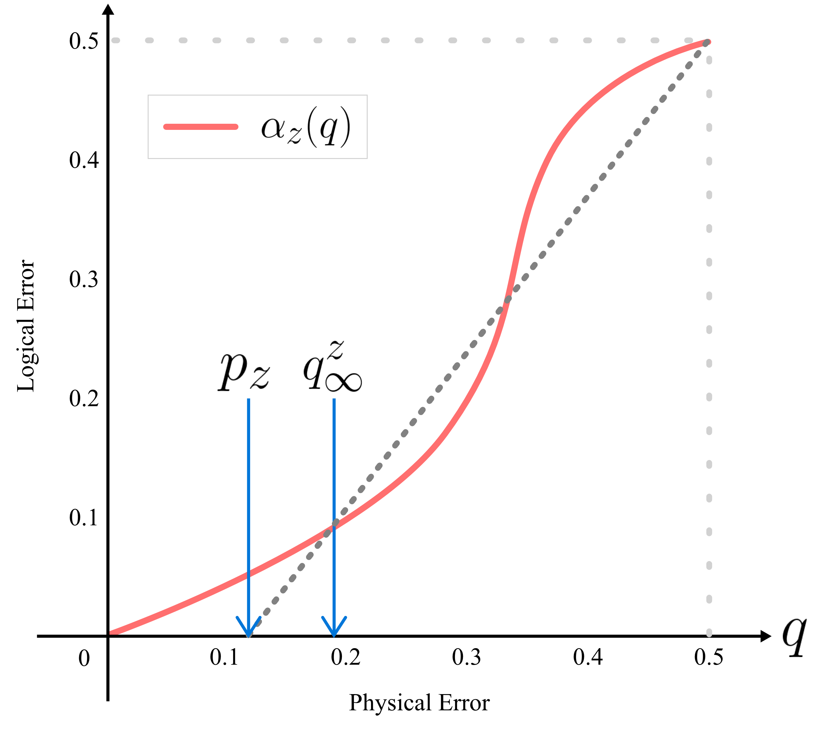
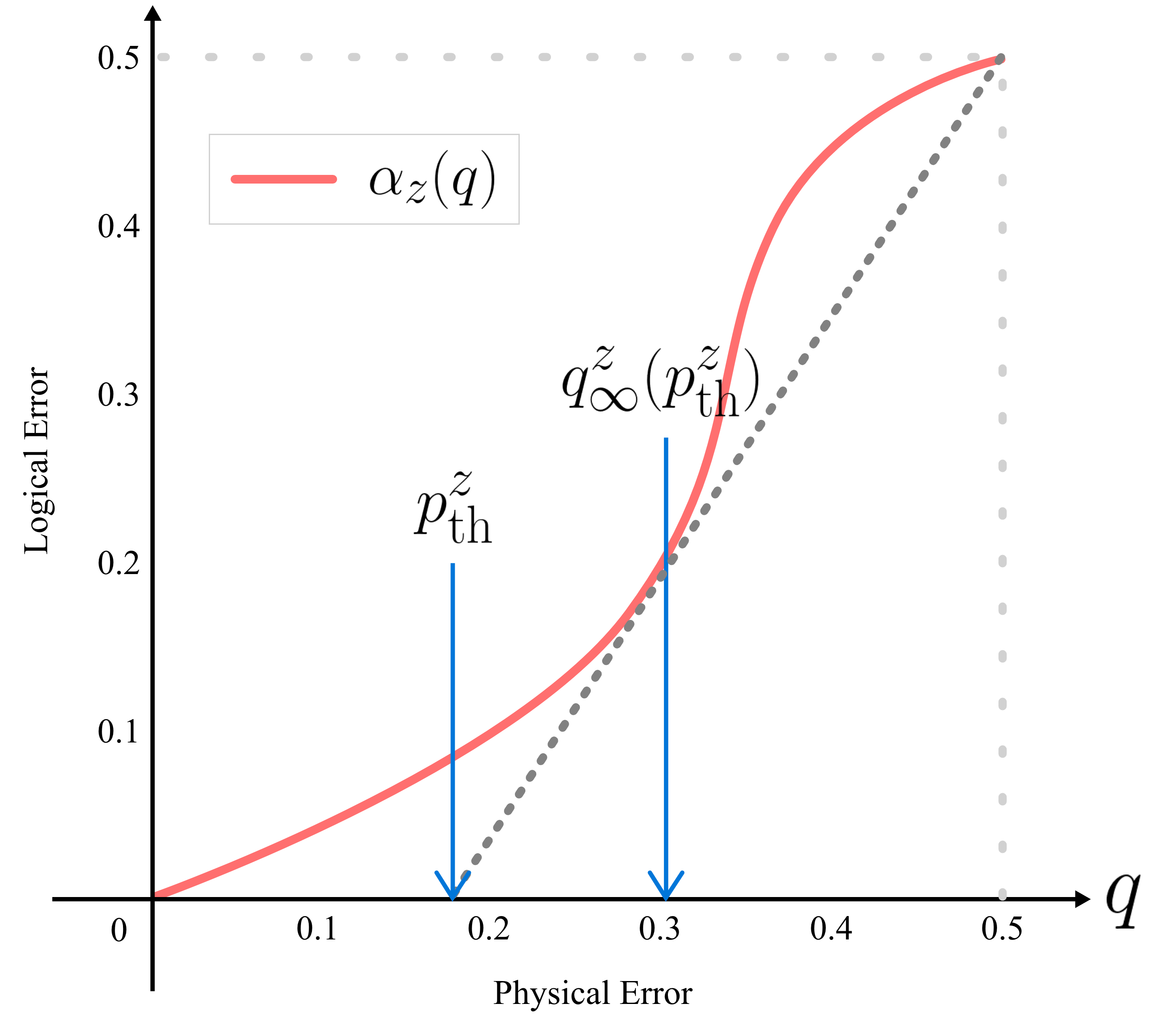
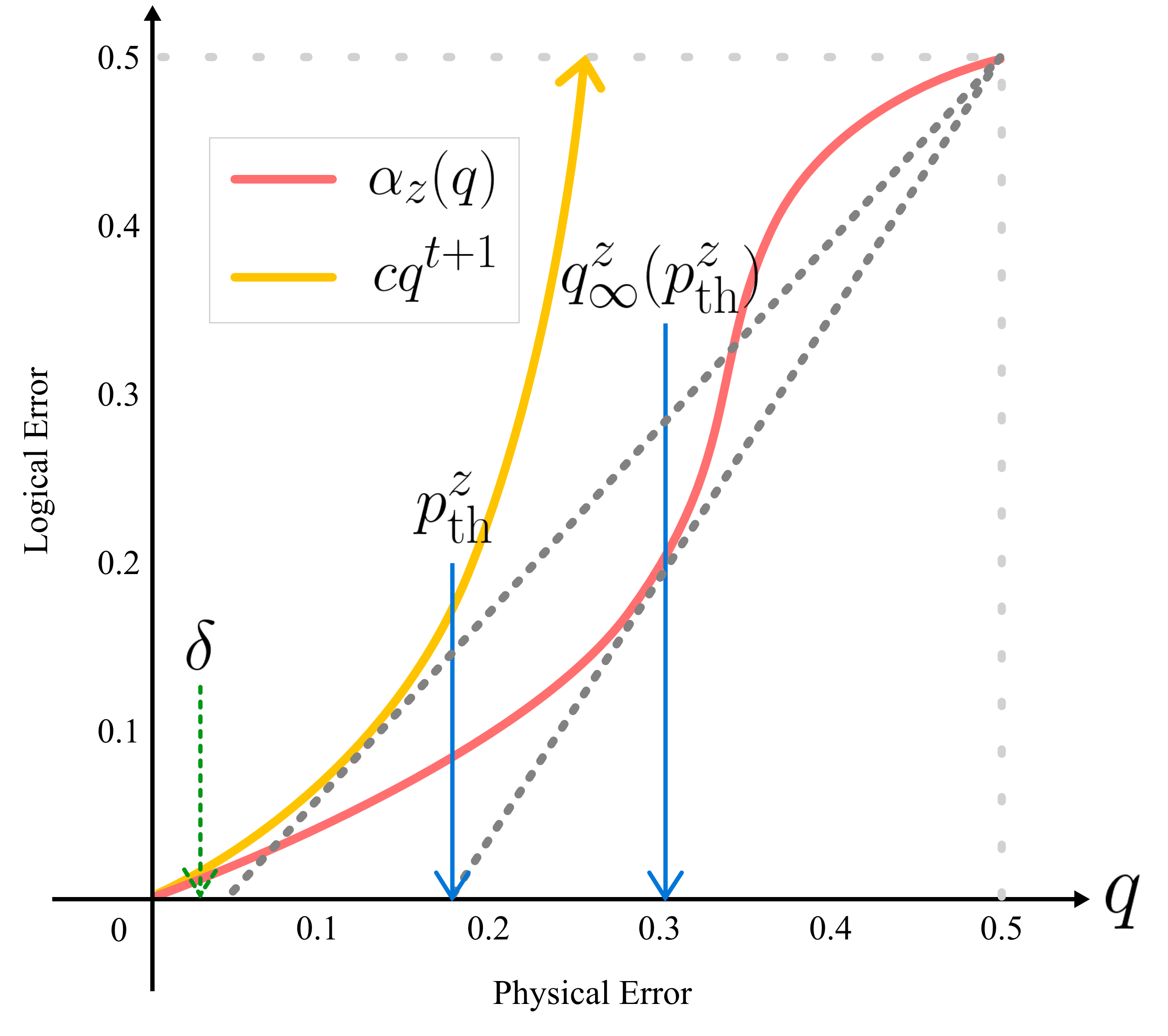
Figure 9: Schematic for recursive decoding threshold computation – The top figure shows the intersection of two curves $\alpha(q)$ and $(q-p_{z})/(1-2p_{z})$, where $p_{z}$ is the error within the tree and the line’s $x$-intercept. According to Eq.(89), for the infinite tree the overall error after the recovery, denoted by $q^{z}_{\infty}$, is determined by the the intersection of these two curves. The smallest $x$-value of the intersections is $q^{z}_{\infty}$. For large enough $p_{z}$, only the $(0.5,0.5)$ intersection persists, entailing that the infinite tree upon local recovery transmits no information. The middle figure shows $p^{z}_{\rm th}$, i.e. the maximum value of $p_{z}$ for which $q^{z}_{\infty}$ is not $0.5$. The bottom figure shows that every $\alpha(q)$ for a $[[b,1,d_{z}]]$ CSS code is upper bounded by $cq^{\lfloor(d_{z}-1)/2\rfloor+1}$, for some constant $2^{t}\leq c\leq 2^{b}$, where $d_{z}\geq d$ is the distance for $Z$ errors. Consider the tangent line to this curve that passes the point $(0.5,0.5)$. The $x$-intercept of this tangent line is a lower bound on $p_{\rm th}^{z}$. Graphically, we see that this lowerbound is always greater than zero. Using this observation, in Appendix C, we show that $p_{\rm th}^{z}$ is lower bounded by $\delta:=\frac{t_{z}}{t_{z}+1}\big{(}\frac{1}{(t_{z}+1)c}\big{)}^{\frac{1}{t_{z}}}$, which is strictly positive when $d_{z}\geq 3$. We also show that for $p_{z}$ less than this value, the logical error in the channel $\widetilde{\mathcal{E}}_{T}=\mathcal{E}_{T}\circ\mathcal{N}$, is bounded by $p_{z}(1+\frac{1}{t_{z}})$.

IV.2.1 Analysis of recursive decoding of CSS code trees
(Proof of Proposition 5)

To analyze the performance of the local recursive strategy for a CSS code tree, we first note that for CSS codes with uncorrelated $X$ and $Z$ errors, error correction for these errors can be performed independently, and therefore after error correction, the $X$ and $Z$ errors remain uncorrelated. In particular, there exists a recovery process $\mathcal{R}$ that corrects $X$ and $Z$ errors independently, i.e., a recovery process $\mathcal{R}$ such that

$$f[\mathcal{M}^{x}\circ\mathcal{M}^{z}]=f[\mathcal{M}^{x}]\circ f[\mathcal{M}^{z}]\ ,$$ (86)

where $\mathcal{M}^{x}$ and $\mathcal{M}^{z}$ are bit-flip and phase-flip channels, respectively, and function $f$ defined in Eq.(74) denotes the effective single-qubit channel after recovery. In particular, if $\mathcal{M}^{z}(\rho)=(1-p)\rho+pZ\rho Z$, then

$$f[\mathcal{M}^{z}](\rho)=(1-\alpha_{z}(p))\rho+\alpha_{z}(p)Z\rho Z\ ,$$ (87)

where $\alpha_{z}(p)$ determines the probability of logical error after recovery. Note that $\alpha_{z}({1}/{2})={1}/{2}$, which corresponds to the cases of maximal $Z$ error. For instance, for the Steane-7 code

$$\alpha_{z}(p)= \ 21p^{2}-98p^{3}+210p^{4}-252p^{5}+168p^{6}-48p^{7}\ .$$

In Appendix D we explain how this function can be calculated for general CSS codes.

Now we consider the recursive Eq.(78) for the phase-flip channel $\mathcal{Q}_{z}$ in Eq.(81), which applies $Z$ error with probability $q_{T}^{z}$. Writing Eq.(78) in terms of function $\alpha_{z}$, we obtain

$$q_{t+1}^{z}=(1-p_{z})\times\alpha_{z}(q_{t}^{z})+p_{z}\times[1-\alpha_{z}(q_{t}^{z})]\ ,$$ (88)

with the initial condition $q_{0}^{z}=p_{z}$. The fixed point of this equation, denoted by $q^{z}_{\infty}$, satisfies

$${\alpha_{z}}(q^{z}_{\infty})=\frac{q^{z}_{\infty}-p_{z}}{1-2p_{z}}\ .$$ (89)

Therefore, to determine $q^{z}_{\infty}$ we study the intersection of the curve ${\alpha}_{z}(q)$ with the line $(q-p_{z})/(1-2p_{z})$ as functions of $q$ (see Fig. 9). Since $\alpha_{z}(1/2)=1/2$, $q^{z}_{\infty}=1/2$ is always a solution. However, for a sufficiently small value of $p_{z}$, the two curves have more intersections in the interval $0<q^{z}_{\infty}<0.5$. Let $p^{z}_{\rm th}$ be the largest value of $p_{z}$ for which they have an intersection in this interval. As it can be seen in Fig. 9 this point is determined by the tangent of curve $\alpha_{z}$ that passes through the point $(0.5,0.5)$. More specifically, $p^{z}_{\rm th}$ is the x-intercept for this line. Given $\alpha_{z}$, $p^{z}_{\text{\rm th}}$ can be estimated numerically.

While the exact threshold $p^{z}_{\text{\rm th}}$ depends on the detail of the polynomial $\alpha_{z}$, its value is strictly positive, provided that the lowest order of $q$ in polynomial $\alpha_{z}(q)$ is 2 or higher, which means the recovery corrects all single-qubit $Z$ errors. This is always possible for codes with distance $d\geq 3$. In particular, suppose the code distance for $Z$ errors is $d_{z}\geq d$, i.e., the code corrects $Z$ errors with weight $t_{z}=\lfloor(d_{z}-1)/2\rfloor$ or less. Then, the lowest order of $q$ in the polynomial $\alpha_{z}(q)$ is $t_{z}+1$. Therefore, there exists a positive constant $c$, such that $\alpha_{z}(q)$ is upper bounded as

$$\alpha_{z}(q)\leq c\times q^{t_{z}+1}\ ,$$ (90)

where $2^{t_{z}}\leq c\leq 2^{b}$ (see Appendix C).

This, in turn, implies that the $x$-intercept of the tangent to $cq^{t_{z}+1}$ lower bounds the $x$-intercept of the tangent to $\alpha_{z}(q)$. Then, using an idea explained in Fig. 9, in Appendix C we show that

$$p^{z}_{\text{th}}\geq\frac{t_{z}}{t_{z}+1}\bigg{(}\frac{1}{(t_{z}+1)c}\bigg{)}^{\frac{1}{t_{z}}}\equiv\delta\ ,$$ (91)

thus, proving the first part of Proposition 5. Furthermore, from Fig. 9 it is clear that for $p_{z}<p^{z}_{\text{th}}$ the overall probability of $Z$ error in the infinite tree, denoted by $q_{\infty}^{z}$ can be arbitrarily small. In particular, we show that $q^{z}_{\infty}\leq p_{z}\times(1+\frac{1}{t_{z}})$.

Finally, to show that $\lim_{p_{z}\rightarrow 0}{q^{z}_{\infty}}/{p_{z}}=1$, consider the Taylor expansion of $q^{z}_{\infty}$ as a function of $p_{z}$ in the limit $p_{z}\rightarrow 0$, as $q^{z}_{\infty}=a_{1}p_{z}+\mathcal{O}(p^{2}_{z})$. Then, on the left-hand side of Eq.(89), the lowest degree of the polynomial $\alpha_{z}(q^{z}_{\infty})$ in $p_{z}$ is larger than or equal to 2, whereas on the right-hand side the lowest-degree term in $p_{z}$ is $(a_{1}-1)\times p_{z}$. Therefore, Eq.(89) implies $a_{1}=1$, hence $\lim_{p_{z}\rightarrow 0}{q^{z}_{\infty}}/{p_{z}}=1$.

IV.3 Example: Noise threshold for recursive decoding of the repetition code tree

Figure 10: Comparing the threshold for the recursive and optimal decoders– Consider a full $b$-ary tree, where each node has the encoder $\ket{c}\mapsto\ket{c}^{\otimes b}:c=0,1$, for odd $b$. Also, assume each edge has a bit-flip channel, which applies Pauli $X$ with probability $p_{x}$. The result of Evans et al. (2000) implies that for the infinite tree, the noise threshold for transmission of classical information in the input $Z$ basis is $p^{\rm opt}_{\text{th}}=\frac{1}{2}(1-\frac{1}{\sqrt{b}})$. Meanwhile, applying the method described in the previous section to the function $\alpha_{\rm maj}$ in Eq.(93), we numerically estimate the local recovery threshold $p_{\rm th}$. The plot shows the ratio $(1-2p_{\rm th})/(1-2p^{\rm opt}_{\rm th})$. For large $b$, this ratio approaches $\sqrt{\pi/2}\approx 1.253$, matching the analytical result in Eq.(94).

As a simple example, we consider the CSS code tree constructed from the standard encoder for the repetition code. Specifically, suppose the encoder at each node is

$$|c\rangle\ \longrightarrow\ V|c\rangle=|c\rangle_{L}=|c\rangle^{\otimes b}\ \ \ :\ c\in\{0,1\}\ ,$$ (92)

for odd integer $b$. Classically the optimal error correction strategy for the repetition code can be realized via majority voting. In the quantum case measuring qubits in $\{|0\rangle,|1\rangle\}$ basis and then performing majority voting destroys coherence between the logical states $|0\rangle_{L}$ and $|1\rangle_{L}$. However, one can perform majority voting in a way that does not destroy this coherence, namely by measuring stabilizers $Z_{j}Z_{j+1}:j=1,\cdots,b-1$. Then, one determines the number of bit-flips (i.e., Pauli $X$) needed to make the eigenvalues of all stabilizers $+1$. There are only two patterns of bit flips that make all the eigenvalues +1. Then, the decoder chooses the one that requires the minimum number of flips. We shall denote this $b\rightarrow 1$ qubit recovery procedure with $\mathcal{R}_{\rm maj}$.

Assuming each qubit is subjected to independent bit-flip error, which flips the bit with probability $p_{x}$, the probability that the decoder makes a wrong guess is given by

$$\alpha_{\rm maj}(p_{x})=\sum_{k={\lfloor b/2\rfloor}+1}^{b}{b\choose k}p_{x}^{k}(1-p_{x})^{b-k}\ .$$ (93)

We can compute the $p_{\rm th}$ as detailed in Sec. IV.2.1. In particular, in Appendix C we show that asymptotically in the limit of large odd $b$

$$p_{\rm th}=\frac{1}{2}\Big{[}1-\sqrt{\frac{\pi}{2}}\frac{1}{\sqrt{b}}\Big{]}+\mathcal{O}(\frac{1}{b})\ .$$ (94)

On the other hand, applying the result of Evans et al. Evans et al. (2000) on broadcasting over classical trees discussed in the introduction, we know that for the optimal recovery the exact threshold is

$$p^{\text{opt}}_{\rm th}=\frac{1}{2}\Big{[}1-\frac{1}{\sqrt{b}}\Big{]}\ .$$ (95)

Interestingly, this threshold can also be achieved via similar majority voting, albeit when it is performed globally on all qubits at the output of the tree, whereas the threshold in Eq.(94) is obtained via recursive local majority voting on groups of $b$ qubits.

In Fig. 10 we compare the actual thresholds for the local and global majority voting approaches for finite values of $b$. See Appendix D for further examples.

V Trees with distance $d=2$ codes:
Recursive decoding with one reliability bit

In this section, we consider trees where at each node the received qubit is encoded in a code with distance $d=2$. Since such codes can not correct single-qubit errors in unknown locations, the local recovery approach discussed in the previous section fails to yield a non-zero threshold for infinite trees: under local recovery, the probability of logical error as a function of the probability of physical error has a linear term, which will then accumulate as the tree depth grows.

To overcome this issue, one may consider a modified version of the recursive recovery that combines several layers together and performs recovery on these combined layers, which corresponds to a concatenated code with distance $d>2$. However, this modification will not solve the aforementioned issue because the noise between the layers still produces uncorrectable logical errors with a probability that is linear in the physical error probability.

To fix this problem, we introduce a new scheme, which takes advantage of the fact that although $d=2$ codes cannot correct errors in unknown locations, they can (i) detect single-qubit errors, and (ii) correct single-qubit errors in known locations. Based on these observations, it is natural to consider a modification of local recovery where each layer sends a reliability bit to the next layer that determines if the decoded qubit is reliable or not. At each layer, the value of this bit is determined based on the value of the reliability bit received from the previous layers together with the syndromes observed in this layer. See Fig. 11 and Sec.V.1 for further details.

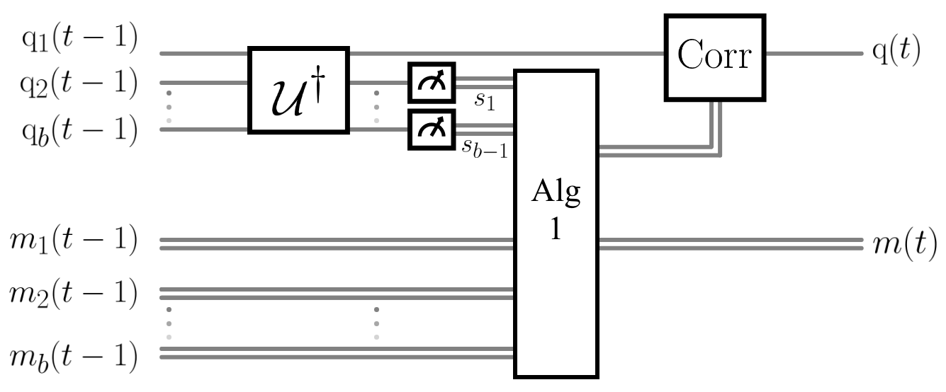
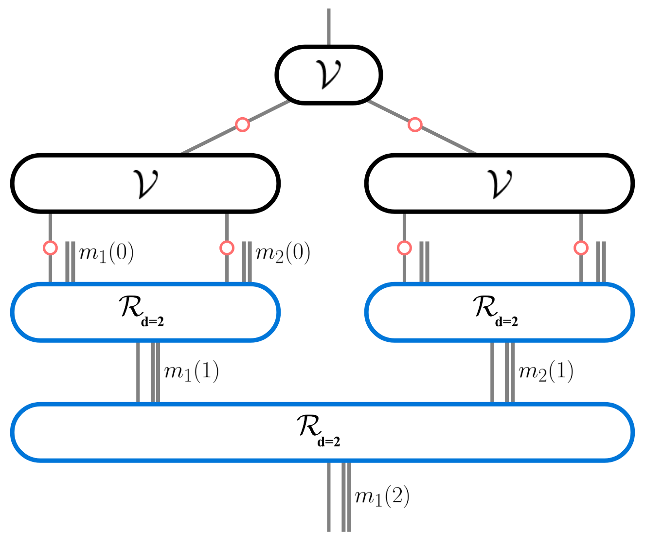
Figure 11: The top figure shows the decoding module for $d=2$ codes with one reliability bit. It first applies the the unitary $\mathcal{U}^{\dagger}$, i.e., the inverse of encoder, on $b$ input qubits $\{{\rm q}_{i}(t-1)\}^{b}_{i=1}$, and then measures $b-1$ ancilla qubits to obtain the syndromes $\{s_{j}\}^{b-1}_{j=1}$. Then, it corrects the logical qubit with a unitary ${\rm Corr}$ controlled by the classical output of Algorithm 1 that classically processes $\{s_{j}\}^{b-1}_{j=1}$ and $\{m_{i}(t-1)\}^{b}_{i=1}$. The exact dictionary between the classical message+syndrome data and the correction unitary is determined by the encoding unitary $\mathcal{U}$. Furthermore, this algorithm also generates the reliability bit $m(t)$ for the subsequent level $t$. The bottom figure presents the action of this decoder for $T=2$ layers.

We rigorously prove and numerically demonstrate that using this recovery it is possible to achieve a noise threshold $p_{\text{th}}$ strictly larger than zero for codes with distance $d=2$. In particular, in Appendix E we show that

Proposition 6.

Consider the tree channel $\mathcal{E}_{T}$ defined in Eq.(9), for a $b$-ary tree of depth $T$. Suppose the noise at each edge is described by the Pauli channel

$$\mathcal{N}(\rho)=(1-p_{\text{tot}})\rho+p_{x}X\rho X+p_{y}Y\rho Y+p_{z}Z\rho Z\ ,$$

where $p_{\text{tot}}=p_{x}+p_{y}+p_{z}$ is the total probability of error. Assume the image of encoder $V:\mathbb{C}^{2}\rightarrow\mathbb{C}^{\otimes b}$ is a stabilizer error-correcting code $[[b,1,2]]$, i.e., a code with distance $2$. Then, for $p_{\text{tot}}<1/(16b^{4}+4b^{2})$, after applying the recovery channel $\mathcal{R}_{T}$ in Sec.V.1, we obtain the Pauli channel

$$\mathcal{R}_{T}\circ{\mathcal{E}}_{T}(\rho)=(1-r^{\text{tot}}_{T})\rho+r^{x}_{T}X\rho X+r^{y}_{T}Y\rho Y+r^{z}_{T}Z\rho Z\ ,$$

with the total probability of logical error $r^{\text{tot}}_{T}=r^{x}_{T}+r^{y}_{T}+r^{z}_{T}$, bounded by

$$r^{\text{tot}}_{T}\leq(1+8b^{2})\times p_{\text{tot}}\ ,$$ (96)

for all $T$.

Indeed, in Appendix E we prove a slightly stronger result: recall that the final output of the recursive decoder in Fig.11 is the decoded qubit along with the corresponding reliability bit $m(T)$ whose value 1 indicates the likelihood of error in the decoded qubit (see subsection V.1 below for further details). We show that if the total physical error is $p_{\text{tot}}<1/(16b^{4}+4b^{2})$ then for all $T$ the probability that the reliability bit $m(T)=1$ remains bounded by $8b^{2}\times p_{\text{tot}}$, and if $m(T)=0$, then the probability of error on the decoded qubit is bounded by $(16b^{4}+4b^{2})\times p_{\text{tot}}^{2}$, hence a quadratic suppression of undetected errors. Then, ignoring the value of the reliability bit $m(T)$, the total probability of error is bounded as Eq.(96).

In conclusion, for $p_{\text{tot}}<1/(16b^{4}+4b^{2})$, the probability of logical error $r^{\text{tot}}_{T}$ is bounded by $(1+8b^{2})/(16b^{4}+4b^{2})$, even for the infinite tree. Since $b\geq 2$, this means $r^{\text{tot}}_{T}\leq\sim 12\%$, which implies that both classical information and entanglement propagate over the infinite tree (see Appendix E).

As a simple example, in Fig. 12 we consider the tree constructed from the binary repetition encoder $|c\rangle\rightarrow|c\rangle|c\rangle\ :c=0,1$, with only bit-flip errors ($p_{z}=p_{y}=0$). Note that technically this code has distance $d=1$. Nevertheless, it detects single-qubit $X$ errors, i.e., it has distance 2 for $X$ errors. Our numerical analysis demonstrates the threshold is $p_{x}\sim 0.125$ which is consistent with the (albeit weak) lowerbound estimate from Proposition 6, $\sim 0.3\%$. Note that in this case the exact threshold can be determined from the result of Evans et al. (2000) on the classical broadcasting problem, namely Eq.(2) which implies $p^{x}_{\text{th}}=(1-1/\sqrt{2})/2\approx 14\%$.

Finally, it is worth noting that for trees with standard or anti-standard encoders of CSS codes with distance 2 with independent $X$ and $Z$ errors on each edge, one can apply the recursive decoding strategy using two reliability bits – one for each type of error – to get improved performance.

Algorithm 1 Decoding module with one reliability bit

begin with $b$ qubits $i=1,...,b$ and their corresponding reliability bits $m_{i}(t-1)$ received from level $t-1$.

apply $\mathcal{U}^{\dagger}$ to the $b$ qubits and measure the $b-1$ ancilla qubits to obtain $\{s_{j}\}_{j}$

if $m_{i}(t-1)=0,\ \forall i$ then

     if $s_{j}=0,\forall j$  then

         $m(t)\leftarrow 0$

     else

         $m(t)\leftarrow 1$

     end if

else if $m_{i}(t-1)=1$ for exactly one $i\in\{1,\cdots,b\}$, denoted as $k$  then

     if $s_{j}=0,\forall j$  then

         $m(t)\leftarrow 0$

     else if some $s_{j}\neq 0$, but $\{s_{j}\}_{j}$ are consistent with error on $k^{\rm th}$ qubit then

         correct logical qubit appropriately

         $m(t)\leftarrow 0$

     else

         $m(t)\leftarrow 1$

     end if

else

     $m(t)\leftarrow 1$

end if

return logical qubit and $m(t)$ to $t$ level.

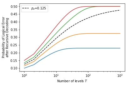
Figure 12: Performance of local recovery with one reliability bit on binary repetition code tree – Suppose each node has the encoder of the binary repetition code, namely $\ket{c}\rightarrow\ket{c}\ket{c}:c=0,1$, and each edge has a bit-flip channel, which applies Pauli $X$ with probability $p_{x}$. The decoder with one reliability bit achieves a non-zero noise threshold for information propagation in infinite trees: when $p_{x}<\sim 0.125$, the logical $X$ error after local recovery of a tree with depth $T\rightarrow\infty$ saturates to strictly below $0.5$, while $p_{x}>\sim 0.125$ ensures the logical $X$ error after recovery saturates to $0.5$.

V.1 Recursive decoding with one reliability bit

Here, we present a full description of the above scheme. Recall that at level $t$ of recursive decoding of a tree of depth $T$, there are $b^{T-t}$ identical blocks each with $b$ qubits inside. Since noise affects all blocks in the same way and the same decoder is applied to all blocks, the following analysis applies to all the blocks at this level. Therefore, to simplify the notation, we suppress the indices that determine the block under consideration, and just label qubits inside a block with index $i=1,\cdots,b$. Let $m_{i}(t-1)$ be the corresponding reliability bits that are received from the previous level (see Fig. 11). In the following, we assume the reliability bit takes the value 1 when the qubit is unreliable or marked. For the first level of recovery, i.e., at the leaves of the tree, we assume the reliability bits are all initiated at $0$.

Now, similar to the original local recovery in the previous section, the recovery starts by applying the inverse of the encoder circuit and then measuring $b-1$ ancilla qubits, which determine the value of syndromes $s_{j}:j=1,\cdots,b-1$. For codes with distance $d=2$ this information is not enough to determine the location of the error. Therefore, unlike the original scheme, the Pauli correction applied to the logical qubit not only depends on these syndromes, but also depends on the value of reliability bits $m_{i}(t-1):i=1,\cdots,b$. More specifically,

1. If no qubit is marked, i.e., $m_{i}(t-1)=0$ for $i=1,\cdots,b$, and no syndrome is observed, i.e., $s_{j}=0$ for all $j=1,\cdots,b-1$, then decode (without applying any correction) and set $m(t)=0$, indicating the reliability of this qubit.

2. Similarly, if exactly one qubit is marked and no syndrome is observed then again decode and set $m(t)=0$.

3. If exactly one qubit is marked and the observed syndromes are consistent with a single-qubit error in that location, then assume there is an error in that location, correct the error, and set $m(t)=0$.

4. In all the other cases, decode ignoring the reliability bits and set $m(t)=1$.

This procedure is also described more precisely in Algorithm 1. Two important remarks are in order here: First, note that only in case 3, the value of the reliability bits affect the applied correction. This is exactly where we take advantage of the fact that codes with distance 2 can correct single-qubit errors in a known location. Secondly, note that if all reliability bits $m_{i}{(t-1)}=0:i=1,\cdots b$ and some error syndromes are observed, while the local recovery cannot correct the error, it sets $m(t)=1$ signaling to the next layer that an error has been detected in this level. In this case, we take advantage of the error detection property of distance 2 codes.

Therefore, assuming the probability that a received qubit at this level has an error with probability $p\ll 1$, the probability that the reliability bit is set to $m(t)=1$ is of order $b\times p$ in the leading order. On the other hand, the probability of an undetected (and thus, unmarked) error is of order $(b\times p)^{2}$. This suppression of the probability of error from order $p$ to $p^{2}$, will make it possible to propagate information over an infinite tree, provided that the probability of physical noise in the single-qubit channels is sufficiently small. In Appendix E, we present a rigorous error analysis for this scheme and prove Proposition 6.

VI Bell Tree – A $d=1$ code tree

Next, we study the Bell tree, introduced in Fig. 2 in the introduction. Here, the encoder is an (anti-standard) encoder of the binary repetition code, which has distance $d=1$: while it can detect a single $X$ error (and correct none), it is fully insensitive to $Z$ errors. Nevertheless, we show that if the probability of $X$ and $Z$ errors are sufficiently small (but non-zero) it is still possible to transmit both classical information and entanglement through the infinite tree. We show this using two different decoders: (i) the optimal decoder which is realized using a belief propagation algorithm discussed in the next section, and (ii) a sub-optimal decoder introduced in this section, which recursively applies a decoding module with two reliability bits (see Fig. 13).

The relatively simple structure of this decoder makes it amenable to both analytical and numerical study. For instance, Fig. 14 presents the results of a numerical study of trees with depth up to $T=1000$, which involves $2^{1000}$ qubits. For this plot, the physical single-qubit noise in the tree channel $\mathcal{E}_{T}$ is $\mathcal{N}=\mathcal{N}_{x}\circ\mathcal{N}_{z}$, where $\mathcal{N}_{x}$ and $\mathcal{N}_{z}$ are bit-flip and phase-flip channels, respectively, which apply $X$ and $Z$ errors, each with probability $p_{x}=p_{z}=p$. This numerical study shows that in the infinite tree for $p<\sim 0.5\%$ the probabilities of logical $Z$ error $q^{z}_{\infty}$ and logical $X$ error $q^{x}_{\infty}$ remain strictly smaller than 0.5; namely $q^{x}_{\infty}\leq 7\%$ and $q^{z}_{\infty}\leq 3\%$. This means that for $p_{x}=p_{z}\lesssim 0.5\%$ both classical information and entanglement propagate to any depth in the Bell tree. Note that although the probability of physical $X$ and $Z$ errors are equal, the probability of logical errors $q^{x}_{T}$ and $q^{z}_{T}$ are not generally equal (see below for further discussion). In addition to these numerical results, in Appendix F we also formally prove the existence of a non-zero threshold for this decoder, and estimate the noise threshold to be lowerbounded by $\sim 0.245\%$, which is consistent with the numerical study.

We also note that the optimal decoder performance for $T=10$ suggests that the actual threshold is lower than $p_{x}=p_{z}\approx 4\%$. It is also worth noting that while the noise threshold for the decoder studied in this section is significantly lower than the actual noise threshold ($\approx 0.5\%$ versus $\approx 4\%$), the performance of the two decoders are similar in the very small noise regime, namely $p_{x}=p_{z}\ll 0.5\%$. Finally, recall that our results in Sec. III.3 imply exponential decay of information for $p_{x}=p_{z}>(1-2^{-1/4})/2\approx 8\%$.

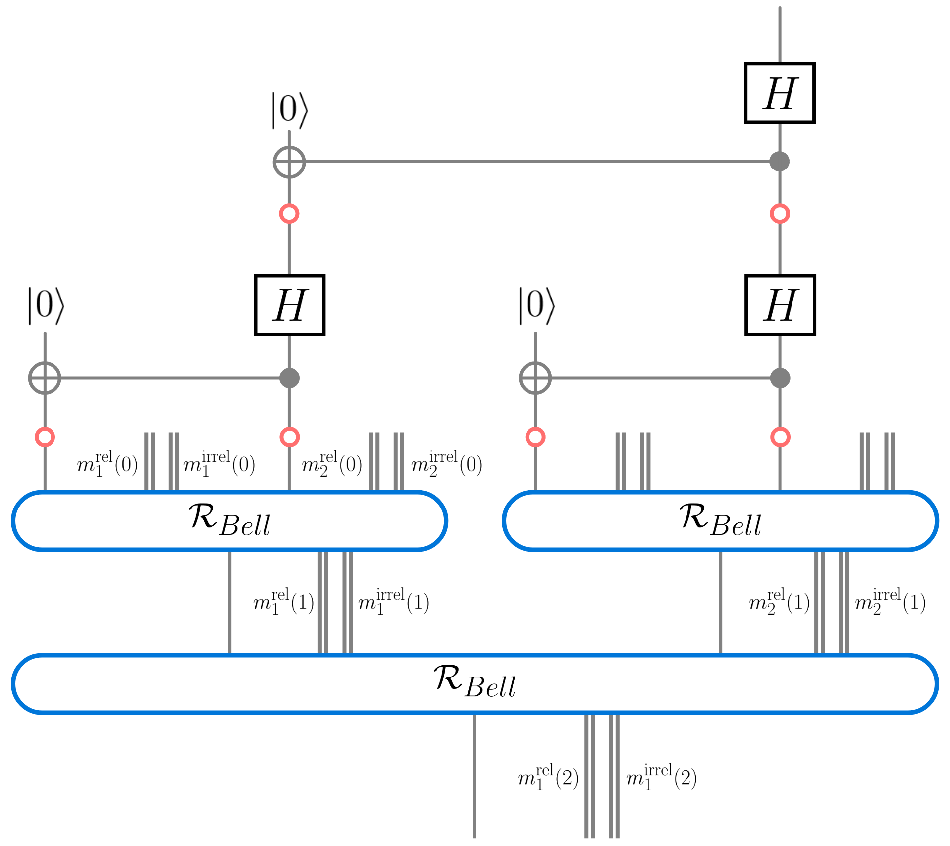
Figure 13: 2 levels of Bell tree and the corresponding recursive decoder: – $\mathcal{R}_{Bell}$ is the decoder module described in Fig.15. Each qubit is augmented with two reliability bites $m^{\text{rel}}(t)$ and $m^{\text{irrel}}(t)$, represented by double lines.

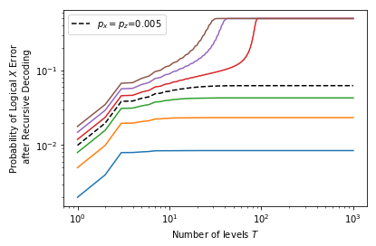
Figure 14: Performance of the recursive decoder with two reliability bits on the Bell trees – We consider the Bell tree with depth $T\rightarrow\infty$ with physical error $p_{x}=p_{z}=p$. For $p<\sim 0.005$, the asymptotic logical $X$ errors after decoding saturates to $q^{x}_{\infty}\leq\sim 0.07$ (a similar result holds for $q^{z}_{\infty}$). On the other hand, for $p>\sim 0.005$ the asymptotic logical $X$ and $Z$ error saturate to $0.5$.

VI.1 Recursive decoding with two reliability bits

Here, we present the full description of the recursive decoder with two reliability bits for the Bell tree. This decoder recursively applies the decoding module with the circuit diagram in Fig.15. The example in Fig.13 presents two layers of this decoder. Recall that at level $t$ of recursive decoding of a Bell tree of depth $T$, there are $2^{T-t}$ identical blocks each with $2$ qubits inside. Since the noise affects all the blocks in the same way and the same decoder is applied to all of them, similar to the previous section, we suppress the indices that determine the block under consideration and just label the two qubits inside a block with index $i=1,2$.

Similar to Algorithm 1, here too the value of the reliability bits at each level is decided based on the observed syndrome and the reliability bits received from the previous level. Each reliability bit determines the likelihood of one type of error, namely $X$ and $Z$ errors, on the decoded qubit. At the first level (i.e., the leaves of the tree) all reliability bits are initiated at 0.

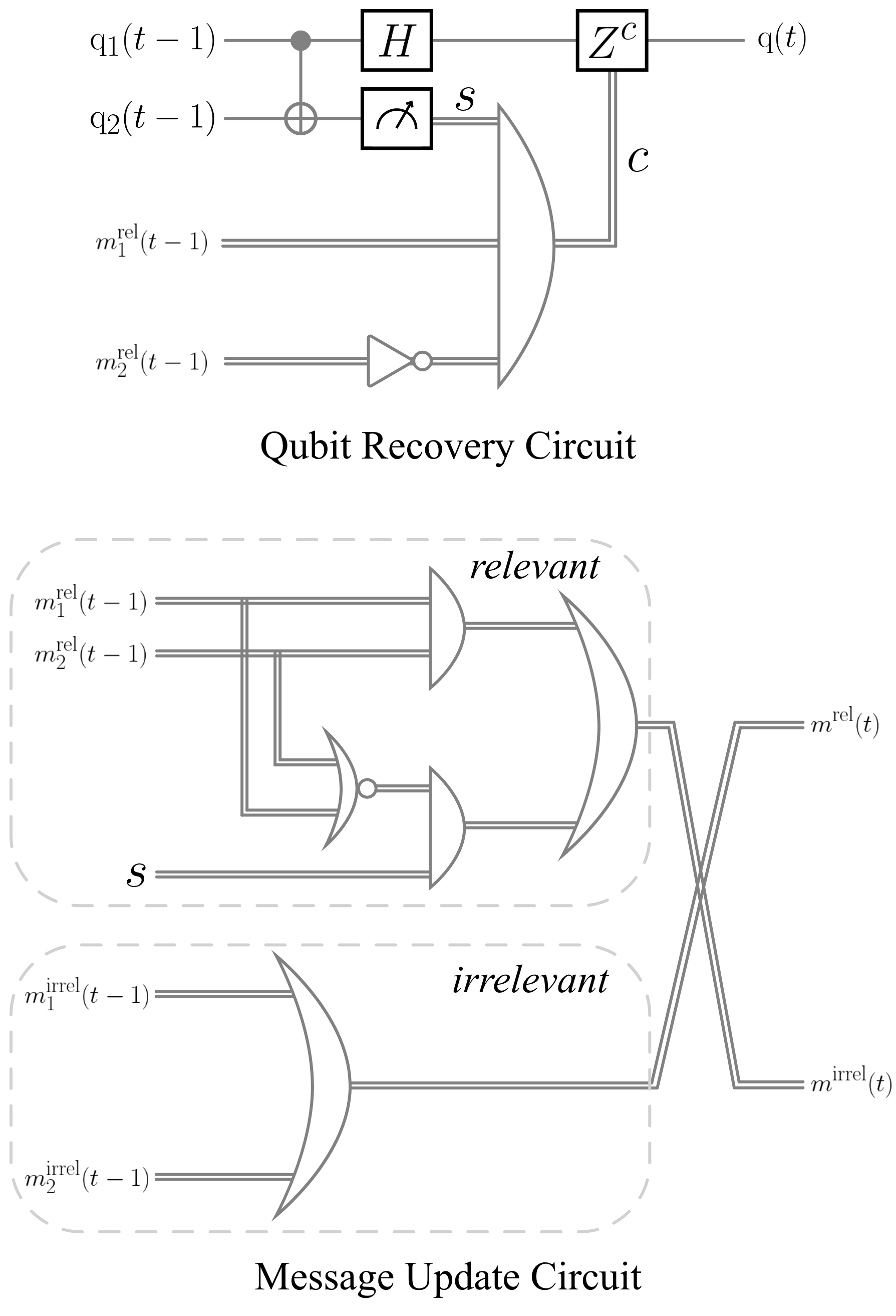
Figure 15: Decoding module for the recursive decoder of the Bell tree – This figure illustrates the three circuits involved in the Bell Tree decoding module from level $t-1$ to $t$. The input to the module are two qubits ${\rm q}_{1}(t-1)$ and ${\rm q}_{2}(t-1)$ along with their ordered reliability bit pairs, labeled as $\{(m^{\text{rel}}_{i}(t-1),m^{\text{irrel}}_{i}(t-1))\}_{i}$ for $i=1,2$. The first figure indicates the decoding circuit that detects the syndrome $s$ and corrects the error based on $m^{\text{rel}}_{i}(t-1):i=1,2$ and $s$. The bottom circuit generates the reliability bits sent to level $t$. It is segmented into relevant and irrelevant parts. The relevant part takes $m^{\text{rel}}_{i}(t-1):i=1,2$ and the syndrome $s$ as the input, whereas the irrelevant part simply is an ${\rm OR}$ function on $m^{\text{irrel}}_{i}(t-1):i=1,2$. Note that the ‘relevant’ and ‘irrelevant’ parts of the decoding module remain separate until the swapping of the bits at the end. This final swap accounts for the fact that the Bell encoder is an anti-standard encoder (see III.3).

Consider the action of the decoding module in Fig.15 on the leaves of the tree. The observed syndrome $s$ determines the outcome of measuring $Z\otimes Z$ stabilizer on the pair of qubits in a block. On the other hand, since the decoding module applies a Hadamard gate on the decoded qubit, the measurement performed in the next level determines the outcome of $X$ stabilizers measured on the leaf qubits. At each level, the decoding module should combine the information obtained from the syndrome measurement with the right type of reliability bits ($X$ or $Z$). This can be achieved, e.g., by adding a third bit that keeps track of the parity of the current level, i.e., whether it is odd or even.

However, in the decoding module in Fig.15, we use a slightly different approach that allows us to avoid the use of this additional bit. Namely, we keep this information in the order of the reliability bits: when qubits $i=1,2$ are received from the level $t-1$, they each come with two reliability bits labeled as relevant and irrelevant bits. The relevant bit is determined by the values of the syndromes at levels $t-2,t-4,\cdots$, which corresponds to the same type of stabilizer that is going to be measured at level $t$ (i.e., $X$ type or $Z$ type).

More precisely, the decoding module in Fig.15 is designed to realize the following rules:

1. Upon receiving qubits 1 and 2, measure the stabilizer $Z_{1}\otimes Z_{2}$ and denote the outcome by $s$.

2. For the pair of received qubits if both relevant reliability bits are zero, i.e., $m_{1}^{\text{rel}}(t-1)\text{ OR }m_{2}^{\text{rel}}(t-1)=0$, and no syndrome is observed ($s=0$), then apply the inverse encoder without applying any correction and set the relevant reliability bit to zero, $m^{\text{rel}}(t)=0$.

3. Similarly, if exactly one relevant reliability bit is 1, i.e., $m_{1}^{\text{rel}}(t-1)\text{ XOR }m_{2}^{\text{rel}}(t-1)=1$, and no syndrome is observed ($s=0$), then apply the inverse encoder without applying any correction and set the relevant reliability bit to 0, i.e., $m^{\text{rel}}(t)=0$.

4. If exactly one relevant reliability bit is 1 and the syndrome is observed (i.e., $s=1$), then assume an error has happened on the marked qubit, correct the error, then apply the inverse encoder and set the relevant reliability bit to 0, i.e., $m^{\text{rel}}(t)=0$.

5. In all the other cases, apply the inverse encoder ignoring the reliability bits and set $m^{\text{rel}}(t)=1$.

6. Set the irrelevant reliability bit to 1 if any of the received irrelevant reliability bits are 1, i.e., $m^{\text{irrel}}(t)=m_{1}^{\text{irrel}}(t-1)\text{ OR }m_{2}^{\text{irrel}}(t-1)$, and then swap the relevant and irrelevant bits.

This procedure is described more precisely in Algorithm 2 in Appendix F, where we also present a rigorous error analysis for this algorithm. It is worth noting that although the circuit in Fig.15 implements the above rules, the order of implementation is slightly different: it first applies the inverse of the encoder and measures the ancilla qubit, and then applies the correction. It is also worth noting that only in case 4, a correction is performed, and after that the reliability bit is set to $m^{\text{rel}}(t)=0$. It is interesting to consider a more “conservative” version of this decoder where in case 4, after the correction the relevant reliability is set to $m^{\text{rel}}(t)=1$, indicating unreliability of the decoded qubit. Numerical results presented in Appendix F suggests that this modification reduces the threshold to around $\sim 0.25\%$, and generally results in a higher probability of logical error.

VII Optimal Decoding with Belief Propagation

Similar to any stabilizer code, the optimal decoding for the concatenated code defined by the tree encoder $V_{T}=\prod_{j=0}^{T-1}V^{\otimes{b}^{j}}$ can be performed by measuring the stabilizer generators. This can be realized by implementing the inverse of this encoder unitary and then measuring all the ancilla qubits in the $Z$ basis. For a tree of depth $T$, this yields a syndrome bitstring $\mathbf{s}_{T}$ of length $b^{T}-1$. In the absence of noise, one obtains the all-zero bit string and the remaining decoded qubit is equal to the input state of the tree. On the other hand, in the presence of an error, the output qubit is equal to the input, upto a logical error $L_{T}=\{I,X,Y,Z\}$. Then, any decoder uses the syndrome $\mathbf{s}_{T}$ to infer $L_{T}$ and correct it by applying $L_{T}$ on the decoded qubit. The optimal decoder needs to find $L_{T}$ that maximizes the conditional probability $p(L_{T}|\mathbf{s}_{T})$. Prima facie, this would require an inefficient double-exponential search over $2^{b^{T}-1}$ distinct values of the syndromes.

However, thanks to the tree structure, it turns out that in the case that is of interest in this paper, the decoding can be performed exponentially more efficiently, in time $\mathcal{O}(2^{T})$. In 2006 Poulin Poulin (2006) developed an efficient algorithm for decoding concatenated codes via belief propagation (BP). This algorithm assumes the encoder is noiseless for the entire concatenated code and the qubits at the leaves of the tree are affected by Pauli errors that are uncorrelated between different qubits. On the other hand, errors between the encoders in the tree, that are considered in this paper, are equivalent to correlated errors on the leaves of the tree. Although the efficient algorithm of Poulin (2006) cannot be extended to general correlated errors, as we explain below, it can be extended to the type of correlated errors that are caused by local errors in between encoders. Roughly speaking, this is possible because such correlations are consistent with the tree structure.

VII.1 Belief Propagation Update Rule

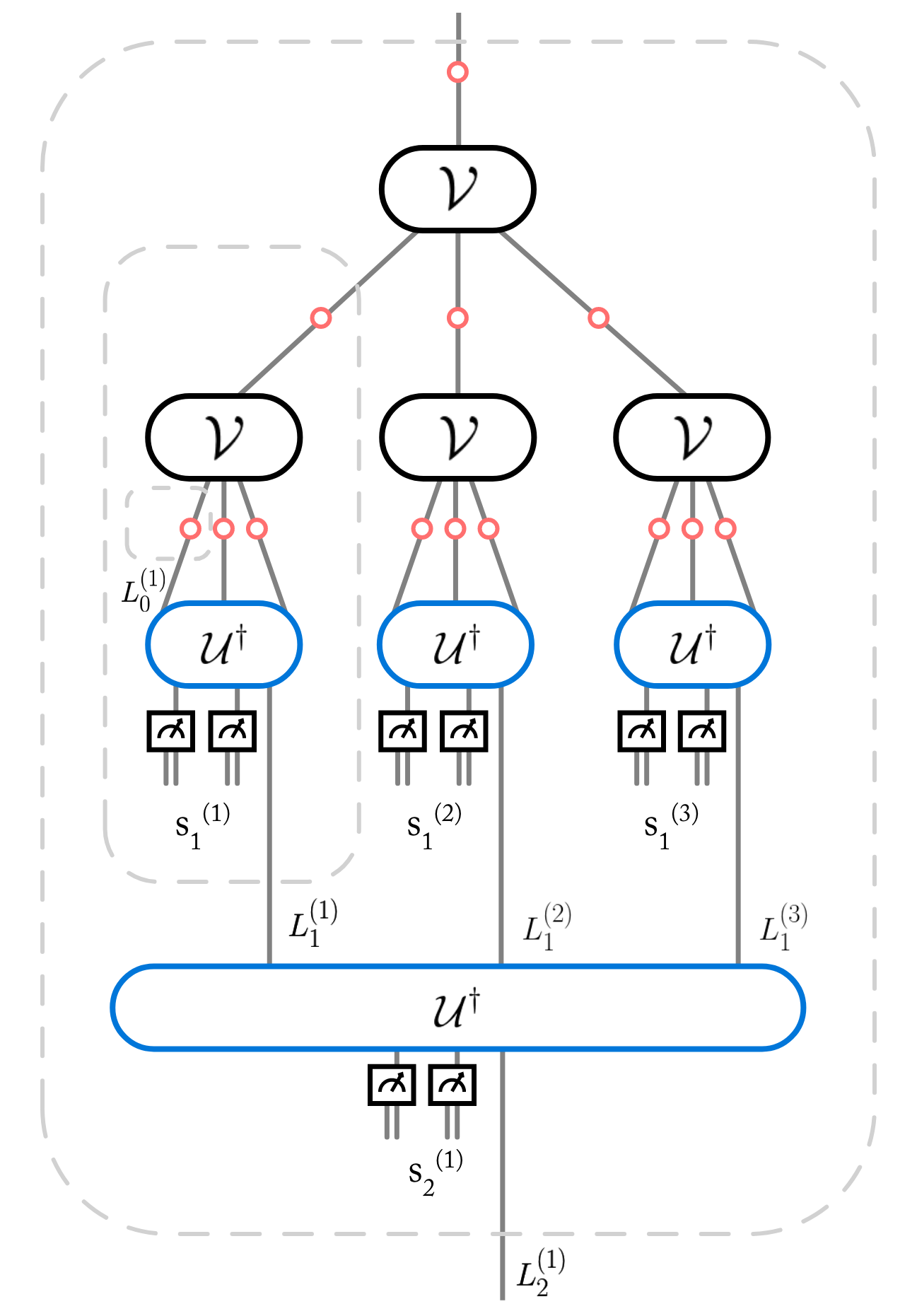
Figure 16: The upper half of the figure is a tree with stabilizer encoder $\mathcal{V}$ along with Pauli noise $\mathcal{N}$ on each edge, which are denoted by red circles. The lower half is the application of the inverse unitaries $U^{\dagger}$ on the output of the tree process (Note that $V|\psi\rangle=U|\psi\rangle|0\rangle^{\otimes(b-1)}$). Upon inversion, each ancillary qubit is measured in the $Z$-basis to obtain the syndromes. $L^{(i)}_{t}\in\{I,X,Y,Z\}$ indicates the overall logical error caused by the noise channels inside the dashed bubble above it, and ${s}^{(i)}_{t}$ is the corresponding syndrome string.

We explain how the algorithm works for the tree of depth $T=2$ with branching number 3, presented in the example in Fig.16. To simplify the presentation, we have considered a tree with noise at the root. Recall that the optimal decoder needs to determine $p(L_{T}|\textbf{s}_{T})$ for the observed value of $\textbf{s}_{T}$. Using the labeling introduced in Fig.16. The goal is to determine

$$p(L_{2}^{(1)}|s_{2}^{(1)},s_{1}^{(1)},s_{1}^{(2)},s_{1}^{(3)})\ .$$

Consider the action of the decoder circuit on the first level. Let error $E$ be an arbitrary tensor product of Pauli operators and the identity operator. Then,

$$U^{\dagger}EU=\mathcal{L}(E)\otimes\mathbf{X}^{{\rm Synd}(E)}\mathbf{Z}^{\mathbf{z}},$$ (97)

where $\mathcal{L}(E)$ is the logical operator acting on the logical qubit and $\mathbf{X}^{{\rm Synd}(E)}$ is the syndrome acting on the ancilla qubits. Since the ancilla is initially prepared in $\ket{0}^{\otimes b-1}$, it remains unchanged under $\mathbf{Z}^{\mathbf{z}}$. We measure and record the syndrome ${\rm Synd}(E)$ in each step of decoding. Furthermore, given Pauli noise channel

$$\mathcal{N}(.)=r_{I}(.)+r_{x}X(.)X+r_{y}Y(.)Y+r_{z}Z(.)Z$$

on the edge prior to the encoder, we define the transition probability between $E_{1}$ and $E_{2}$ in the Pauli group as

$$N(E_{1}|E_{2})=r_{E_{1}E_{2}}\ ,$$ (98)

where $E_{1}E_{2}$ is the matrix product of Pauli operators $E_{1}$ and $E_{2}$ upto a global phase.

The key point is $p(L^{(1)}_{2}|s_{2}^{(1)},s_{1}^{(1)},s_{1}^{(2)},s_{1}^{(3)})$ has a decomposition as

$$p (L^{(1)}_{2}|s_{2}^{(1)},s_{1}^{(1)},s_{1}^{(2)},s_{1}^{(3)})$$

$$=\frac{1}{p(s^{(1)}_{2}|\mathbf{s}_{1})}\sum_{\textbf{L}_{1}}f_{s^{(1)}_{2}}(L^{(1)}_{2},\textbf{L}_{1})\times\prod^{3}_{i=1}p(L^{(i)}_{1}|{s}^{(i)}_{1})\ ,$$ (99)

where $\textbf{L}_{1}=L^{(1)}_{1}L^{(2)}_{1}L^{(3)}_{1}$, $\mathbf{s}_{1}=s^{(1)}_{1}s^{(2)}_{1}s^{(3)}_{1}$ and

$$f_{s^{(1)}_{2}}(L^{(1)}_{2},\textbf{L}_{1}):=\delta[s^{(1)}_{2}={\rm Synd}(\textbf{L}_{1})]\times N(L^{(1)}_{2}|\mathcal{L}(\textbf{L}_{1})).$$

Notice that conditioned on $s^{(i)}_{1}$, the logical error $L^{(i)}_{1}$ is independent of the rest of the syndrome bits, which is clear from the tree structure. Now, this formula can be reapplied to $p(L^{(i)}_{1}|s^{(i)}_{1})$ for each $i$. For instance, for the $i=1$ subtree we have

$$p(L^{(1)}_{1}|s^{(1)}_{1})=\sum_{\textbf{L}_{0}}f_{s^{(1)}_{1}}(L^{(1)}_{1},\textbf{L}_{0})\frac{1}{p(s^{(1)}_{1})}\times\prod_{i=1}^{3}p(L^{(i)}_{0})$$ (100)

where $\textbf{L}_{0}=L^{(1)}_{0}L^{(2)}_{0}L^{(3)}_{0}$, and the superscript labels the three leaves in the first subtree. We can repeat this for the other two trees as well. At this point, we have reached level $0$, i.e., the leaves of the tree. Therefore, when $p(L^{(i)}_{0})$ appears in the expression, we have reached the terminal condition for recursion and we set $p(L^{(i)}_{0})=N(L^{(i)}_{0}|I)=r_{L^{(i)}_{0}}$. See Appendix G for further details of this algorithm for general stabilizer trees. In the following, we present some numerical results.

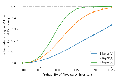
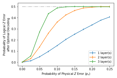
Figure 17: Optimal recovery of Shor-9 tree. Probability of logical error as a function of the probability of physical error in the tree for trees of depth $T=1,2$ and $3$. In the top plot, the $y$-axis indicates the overall logical $X$-error after optimal decoding given the physical $X$ noise within the tree has probability $p_{x}$ indicated on the $x$-axis. The bottom plot shows the same quantities for $Z$ errors. This provides improved upperbound estimates for noise threshold for $X$ errors at $\sim 0.17$, and for $Z$ errors at $\sim 0.13$. Each data point in the plots is computed via a Monte Carlo of $10^{5}$ samples explain in Appendix G.8.

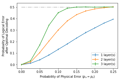
Figure 18: Optimal recovery of Steane-7 tree. Probability of logical error as a function of the probability of physical error for trees of depth $T=1,2,3$. Note that since Steane-7 code is self-dual $X$ and $Z$ errors have the same behavior, and therefore this plot presents both cases. In particular, $x$ axis is the probability $p_{x}=p_{z}$ of physical error in the channel. This provides upperbound estimates for asymptotic noise threshold for $X/Z$ error at $p\sim 0.15$. Each data point in the plots is computed via a Monte Carlo of $10^{5}$ samples explained in Appendix G.8.

VII.2 Examples

Shor-9 Code

Fig. 17 plots the logical error for the tree as defined in Eq.(9) constructed from a Shor-9 code encoder that is standard in both $X$ and $Z$. We consider trees of depths $T=1,2,3$. The specifics of constructing this plot are explained in Appendix G.8. We see that the asymptotic noise threshold for $X$ errors is below $\sim 0.17$, whereas for $Z$ errors it is below $\sim 0.13$ (since the number of $Z$ stabilizers in the Shor-9 code is higher than $X$ stabilizers and therefore this code is better equipped to correct $X$ errors than $Z$ errors). Recall that our result in Proposition 1 establishes an upper bound $\sim 0.21$; thus, these numerics provide evidence for a tighter bound for the noise threshold.

After optimal recovery for channel $\mathcal{E}_{T}$, the overall channel is a composition of a bit-flip and a phase-flip channel with the probability of $X$ error and $Z$ errors $q_{x}^{T},q^{T}_{z}\leq 1/2$, respectively. Such channels are entanglement-breaking if, and only if, $|1-q_{T}^{z}|\times|1-q_{T}^{x}|<1/2$ (see Appendix B.2). From numerical results in Fig.17, it follows that for depth $T=3$, this condition is satisfied for $p>\sim 0.07$. Note that since the error monotonically increases with $T$, the same also holds for $T\geq 3$.

Steane-7 Code

Fig. 18 plots the optimal recovery performance for a tree as defined in Eq.(9) composed of Steane-7 encoders that are standard in both $X$ and $Z$, and is similarly subject to independent $X$ and $Z$ errors for depths $T=1,2,3$. Specifics of this recovery procedure are detailed in Appendix G.9. Here, we see that the asymptotic noise threshold for $X$ errors is below $\sim 0.15$. Because the Steane-7 code is self-dual, the same threshold holds true for the $Z$ errors as well. Using an argument similar to the Shor-9 code, one can show that for $p>\sim 0.07$, entanglement cannot be transmitted beyond depth $T\geq 3$.

VIII Mapping Quantum trees to classical trees with correlated errors

In this section, we argue that stabilizer trees can be understood in terms of an equivalent classical problem, which is a variant of the standard broadcasting problem on trees discussed in the introduction. For simplicity, we focus on trees constructed from a standard encoder of a CSS code with independent phase-flip and bit-flip channels.

Suppose we modify the original channel $\mathcal{E}_{T}$ defined in Eq.(9), by adding a fully dephasing channel $\mathcal{D}_{z}$ before and after each encoder. That is, at each node we modify the encoder $\mathcal{V}$ to

$$\mathcal{V}\ \ \ \longrightarrow\ \ \ \overline{\mathcal{V}}\equiv\mathcal{D}_{z}^{\otimes b}\circ\mathcal{V}\circ\mathcal{D}_{z}\ .$$ (101)

Then, the channel $\mathcal{E}_{T}$ defined in Eq.(9) will be modified to

$$\overline{\mathcal{E}}_{T}(\rho)=\prod_{j=0}^{T-1}{\overline{\mathcal{V}}}^{\otimes b^{j}}\circ\mathcal{N}^{\otimes b^{j}}(\rho)\ ,$$ (102)

which will be called the dephased tree in the following. Equivalently, rather than inserting dephasing channels $\mathcal{D}_{z}$, we can assume the probability of $Z$ error $p_{z}$ is increased to 1/2.

Then, at any level of the tree the density operator of qubits will be diagonal in the computational basis. In particular, the action of the dephased encoder $\overline{\mathcal{V}}$ is fully characterized by the classical channel with the conditional probability distribution

$$P_{z}(\textbf{z}|c)=\langle\textbf{z}|\mathcal{V}(|c\rangle\langle c|)|\textbf{z}\rangle\ \ \ \ \ :\ c=0,1\ ,\ \textbf{z}\in\{0,1\}^{b}\ \ .$$ (103)

Note that the property that the density operator is diagonal in the computational basis remains valid under Pauli errors. In particular, $Z$ errors act trivially on such states, whereas $X$ errors, i.e., bit-flip channels, become a binary symmetric channel, which can described by the conditional probability

$$N_{z}(j|i)=p_{x}+(1-2p_{x})\delta_{i,j}\ \ \ :\ i,j=0,1\ .$$ (104)

Therefore, by adding dephasing before and after each encoder, as described in Eq.(101), we obtain a fully classical problem: at each node, a bit $c\in\{0,1\}$ enters the encoder, and at the output of the encoder a bit string $\textbf{z}\in\{0,1\}^{b}$ with probability $P(\textbf{z}|c)$ is generated. Then, each bit goes into a binary symmetric channel $Q$, which flips the input bit with probability $p_{x}$ and leaves it unchanged with probability $1-p_{x}$. Finally, each bit goes to the next level and enters another encoder $\overline{\mathcal{V}}$.

The assumption that the encoder at each node is a standard encoder implies that the effect of inserted dephasing channels $\mathcal{D}_{z}$ in the middle of the tree is equivalent to correlated $Z$ errors on the leaves. Furthermore, because for CSS codes $Z$ and $X$ errors can be corrected independently, we conclude that the probability of logical $X$ error, $q_{T}^{x}$ for the dephased channel $\overline{\mathcal{E}}_{T}$ and the original channel ${\mathcal{E}}_{T}$ are equal. Another way to phrase this observation is to say that the distinguishability of the output states $\mathcal{E}_{T}(|0\rangle\langle 0|)$ and $\mathcal{E}_{T}(|1\rangle\langle 1|)$ with respect to any measure of distinguishability, such as the trace distance, is the same as the distinguishability of states $\overline{\mathcal{E}}_{T}(|0\rangle\langle 0|)$ and $\overline{\mathcal{E}}_{T}(|1\rangle\langle 1|)$. To prove this it suffices to show that there exists a channel $\mathcal{T}_{T}$ such that

$$\mathcal{T}_{T}\circ\overline{\mathcal{E}}_{T}(|c\rangle\langle c|)=\mathcal{E}_{T}(|c\rangle\langle c|)\ \ \ :c=0,1\ .$$ (105)

A channel $\mathcal{T}_{T}$ that satisfies the above equation is the error correction of $Z$ errors, which requires measuring $X$ stabilizers and correcting the $Z$ errors based on the outcomes of the measurement, followed by adding certain (correlated) $Z$ errors to reproduce the effect of $Z$ errors in $\mathcal{E}_{T}$ (see proposition 11 in Appendix H). Note that instead of the $Z$ basis, we can dephase qubits in the $X$ basis. This results in another classical tree with depth $T$, which can be used to determine the probability of logical $Z$ error $q_{T}^{z}$. Similarly, in the case of CSS codes with anti-standard encoders the equivalent classical tree can be obtained by measuring the qubits in the $Z$ and $X$ bases, alternating between different levels (see the example below).

We conclude that any CSS tree with standard or anti-standard encoders and independent $X$ and $Z$ errors can be fully characterized in terms of a modification of the classical broadcasting problem which involves correlated noise on the edges that leave the same node. As an example, here we consider the classical tree corresponding to the Shor 9-qubit code. See Appendix H.1 for further examples.

VIII.1 Example: Bell Tree

Consider the Bell tree discussed in Sec.(VI) with noise rate $p_{x}=p_{z}=p$. Recall that the Bell encoder is an anti-standard encoder. Thus, as mentioned above, we must dephase alternatingly in the $X$ and $Z$ bases. Suppose we are interested in the propagation of information encoded in $Z$ eigenstates (i.e., $\{\ket{0},\ket{1}\}$) of the input. Then, we shall dephase the root of the tree in the $Z$ direction, then the next level must be dephased in the $X$ direction, and so on. This implies that the dephased versions of two levels of a Bell tree is the concatenation of two kinds of classical encoders

$$\mathbb{M}_{1}: \ P_{z}(00|0)=1$$

$$\ P_{z}(11|1)=1$$ (106)

$$\mathbb{M}_{2}: \ P_{z}(\mathbf{w}|0)=1/2,\ {\rm when}\ \mathbf{w}\in\{00,11\}$$

$$\ P_{z}(\mathbf{w}|1)=1/2,\ {\rm when}\ \mathbf{w}\in\{01,10\}$$ (107)

that are present on alternate levels of the tree. For instance, the dephased version of a $T=2$ Bell tree (as seen in Fig. (2) is,

$$\mathbb{N}^{\otimes 4}\circ\mathbb{M}_{1}^{\otimes 2}\circ\mathbb{N}^{\otimes 2}\circ\mathbb{M}_{2}\ ,$$ (108)

where $\mathbb{N}$ represents the classical bit-flip channel that flips the input bit with

VIII.2 Future Directions

This paper opens up several lines of inquiry. For instance, finding the exact noise threshold for the propagation of classical information and entanglement in an infinite tree remains an open question. In particular, it will be interesting to see if the classical information-theoretic arguments based on strong data-processing inequality Evans and Schulman (1999); Polyanskiy and Wu (2017); Cao and Lu (2019) can be generalized to the quantum setting.

A natural extension of this work is to consider other (non-Clifford) encoders and noise processes. In particular, the case of Haar-random (independent) unitaries Dalzell et al. (2021); Deshpande et al. (2022) at different nodes is an interesting model for natural processes. Other noise models such as erasure noise or coherent noise can also be studied. While the current study assumes that the decoder has access to all the exponentially many qubits at the end of the tree, more pragmatically one can study how classical and quantum correlations are affected when we consider only a subset of the leaves instead of all of them. A thorough study of classical trees obtained by dephasing quantum trees (as explained in Sec.H.2) is an open question not just of independent interest within classical network theory, but with direct applications to CSS code trees. Finally, some ideas presented in this paper can have applications for more general quantum networks described by directed acyclic graphs.

Appendix

Appendix A Quick review of the relevant results on classical trees

In this appendix, we briefly review a result presented in Evans et al. (2000) and Mossel and Peres (2003) that upperbounds the information propagation down noisy trees.

Consider a tree network $\Gamma$ where a certain node/vertex has been chosen to be the root. This choice allows us to view the tree as a directed graph where bits stream from the root to the leaves. Every vertex is characterized by a branching number, which is the number of outgoing edges (vertices of a tree always have one incoming edge). Every vertex $\mathbf{v}$ defines a copier bit-process where $0\mapsto 0^{\otimes b}$ and $1\mapsto 1^{\otimes b}$, where $b$ is the number of children at the vertex $\mathbf{v}$. Additionally, each edge $\mathbf{e}$ is associated to a single bit-flip with probability $p_{\mathbf{e}}$. We also define $\theta_{\mathbf{e}}:=1-2p_{\mathbf{e}}$.

Let us assume the root bit is $x_{0}$. At the end of this tree process $\Gamma$, the probability of obtaining bitstring $\overline{x}_{T}$ at level $T$ is ${\rm p}_{\mathbf{T}}(\overline{x}_{T}|x_{0})$ where we conditioned by the root value $x_{0}$. The information propagated via $\Gamma$ is quantified by the total variation distance,

$$\Delta\equiv\frac{1}{2}||{p}(\mathbf{x}_{T}|\mathbf{x}_{0}=0)-{p}(\mathbf{x}_{T}|\mathbf{x}_{0}=1)||_{1}=\frac{1}{2}\sum_{\mathbf{x}_{T}}|{p}(\mathbf{x}_{T}|\mathbf{x}_{0}=0)-{p}(\mathbf{x}_{T}|\mathbf{x}_{0}=1)|.$$ (109)

To upperbound this quantity, we first define,

$$\Theta_{\mathbf{e}}:=\prod_{\mathbf{e}^{\prime}\in[\mathbf{e}]}\theta_{\mathbf{e}^{\prime}}$$ (110)

where $[\mathbf{e}]$ is the set of all edges in the path between the root and edge $\mathbf{e}$, including the ends. Because of the tree structure, we are ensured a unique path between the root and any edge $\mathbf{e}$. Theorem 1.3’ in Evans et al. (2000) states that,

$$\Delta^{2}\leq 2\sum_{\mathbf{e}\in\mathbf{W}_{T}}\Theta^{2}_{\mathbf{e}}$$ (111)

where the summation is over the set $\mathbf{W}_{T}$ that contains all edges at level $T$ of the tree. This statement is proved in Evans et al. (2000) using a domination argument where they show that a ‘stringy’ tree can be post-processed by appropriate stochastic maps to simulate the original tree process. Thus, benchmarking the ‘stringy’ tree gives an upperbound on the original tree’s performance due to data processing inequality. The ‘stringy’ is, thus, chosen to be one for whom the TVD is very easy to compute, yielding the above upperbound.

Suppose the error probability on each edge is $p$ and there are $n_{T}$ edges in level $T$. Then this formula simplifies to

$$\Delta\leq\sqrt{2}\times\sqrt{n_{T}}\times(1-2p)^{T}$$ (112)

Furthermore, consider the important special case of a full $b$-ary tree where every vertex has uniform branching number $b$, and all bit-flip probabilities across edges are the same, $p$. After $T$ levels, we have that $n^{T}=b^{T}$. So,

$$\Delta\leq\sqrt{2}\times(\sqrt{b}(1-2p))^{T}.$$ (113)

This is the result presented in Eq.(13) of Evans et al. (2000). This upperbound provides an asymptotic noise threshold upperbound of $p_{\rm th}\leq\frac{1}{2}(1-\frac{1}{\sqrt{b}})$. This square-root scaling upperbound is sometimes referred to as Kesten-Stigum bounds. Evans et al. (2000); Mossel and Peres (2003) demonstrate that this upperbound is also the lowerbound for the noise threshold, rendering it the critical noise threshold for classical trees.

Appendix B Review of some useful facts about Pauli channels

Here, we briefly review some useful facts about the Diamond norm distance of Pauli channels and the condition for entanglement-breaking Pauli channels. See, e.g., Wilde (2013); Horodecki et al. (2003) for further discussion and references.

B.1 Diamond norm distance between Pauli Channels

Recall that the diamond norm of a super-operator ${\Phi}$ that acts on operators in the system $S$ with Hilbert space $\mathcal{H}_{S}$ is defined as

$$\|{\Phi}\|_{\diamond}=\max_{\rho_{SR}}\|{\Phi}\otimes{\rm id}_{R}(\rho_{SR})\|_{1}\ ,$$ (114)

where $R$ is a reference system with Hilbert space $\mathcal{H}_{R}$ such that ${\rm dim}(\mathcal{H}_{R})={\rm dim}(\mathcal{H}_{S})$, and ${\rm id}_{R}$ is the identity super-operator on $\mathcal{H}_{R}$. The maximization is over all states in the composite system $SR$, i.e., $\mathcal{H}_{S}\otimes\mathcal{H}_{R}$. We use the diamond norm to quantify the distance between two channels.

Lemma 7.

Consider two n-qubit Pauli channels, namely

$$\mathcal{P}(\cdot) =\sum_{\mathbf{x},\mathbf{z}\in\{0,1\}^{n}}p(\mathbf{x},\mathbf{z})\ \mathbf{X}^{\mathbf{x}}\mathbf{Z}^{\mathbf{z}}(.)\mathbf{Z}^{\mathbf{z}}\mathbf{X}^{\mathbf{x}}$$

$$\mathcal{Q}(\cdot) =\sum_{\mathbf{x},\mathbf{z}\in\{0,1\}^{n}}q(\mathbf{x},\mathbf{z})\ \mathbf{X}^{\mathbf{x}}\mathbf{Z}^{\mathbf{z}}(.)\mathbf{Z}^{\mathbf{z}}\mathbf{X}^{\mathbf{x}}.$$

The diamond distance of the channels is equal to the total variation distance of the corresponding probability distributions

$$d_{\diamond}(\mathcal{P},\mathcal{Q})=\frac{1}{2}\|\mathcal{P}-\mathcal{Q}\|_{\diamond}=\frac{1}{2}\sum_{\mathbf{x},\mathbf{z}}|p(\mathbf{x},\mathbf{z})-q(\mathbf{x},\mathbf{z})|\ .$$

Proof.

We prove this statement by lower and upperbounding by the TVD. The upperbound follows from triangle inequality for diamond norm, namely

$$||\mathcal{P}-\mathcal{Q}||_{\diamond}=\|\sum_{\mathbf{x},\mathbf{z}}[p(\mathbf{x},\mathbf{z})-q(\mathbf{x},\mathbf{z})]\mathbf{X}^{\mathbf{x}}\mathbf{Z}^{\mathbf{z}}(\cdot)\mathbf{X}^{\mathbf{x}}\mathbf{Z}^{\mathbf{z}}\|_{\diamond}\leq\sum_{\mathbf{x},\mathbf{z}}|p(\mathbf{x},\mathbf{z})-q(\mathbf{x},\mathbf{z})|\times\|\mathbf{X}^{\mathbf{x}}\mathbf{Z}^{\mathbf{z}}(\cdot)\mathbf{X}^{\mathbf{x}}\mathbf{Z}^{\mathbf{z}}\|_{\diamond}=\sum_{\mathbf{x},\mathbf{z}}|p(\mathbf{x},\mathbf{z})-q(\mathbf{x},\mathbf{z})|\ .$$ (115)

To show that this bound holds as an equality, it suffices to show that there exists a state $\rho_{RS}$ such that $\|(\mathcal{P}-\mathcal{Q})\otimes{\rm id}_{R}(\rho_{SR})\|_{1}$ is equal to the right-hand side. Inspired by the super-dense coding protocol, which allows perfect discrimination of Pauli operators using maximally entangled states, we consider the maximally entangled state $\ket{\Psi}=\frac{1}{\sqrt{2^{n}}}\sum_{\mathbf{i}}\ket{\mathbf{i}}\otimes\ket{\mathbf{i}}$, where the summation $\mathbf{i}$ is over all bitstrings of length $n$. Then we have,

$$||\mathcal{P}-\mathcal{Q}||_{\diamond}= \max_{\rho_{SR}}||\sum_{\mathbf{x},\mathbf{z}}[p(\mathbf{x},\mathbf{z})-q(\mathbf{x},\mathbf{z})]\ \mathbf{X}^{\mathbf{x}}\mathbf{Z}^{\mathbf{z}}\otimes I_{R}(\rho_{SR})\mathbf{Z}^{\mathbf{z}}\mathbf{X}^{\mathbf{x}}\otimes I_{R}||_{1}$$ (116)

$$\geq ||\sum_{\mathbf{x},\mathbf{z}}[p(\mathbf{x},\mathbf{z})-q(\mathbf{x},\mathbf{z})]\ \mathbf{X}^{\mathbf{x}}\mathbf{Z}^{\mathbf{z}}\otimes I_{R}(|{\Psi}\rangle\!\langle\Psi|)\mathbf{Z}^{\mathbf{z}}\mathbf{X}^{\mathbf{x}}\otimes I_{R}||_{1}$$ (117)

As we expect from super-dense coding, the set of states, $\{\mathbf{X}^{\mathbf{x}}\mathbf{Z}^{\mathbf{z}}\otimes I_{R}\ket{\Psi}\}_{\mathbf{x},\mathbf{z}}$ indexed by $\mathbf{x},\mathbf{z}$ are orthonormal. To see this, consider $\mathbf{x}\neq\mathbf{x}^{\prime}$ and/or $\mathbf{z}\neq\mathbf{z}^{\prime}$,

$$\bra{\Psi}[\mathbf{X}^{\mathbf{x}}\mathbf{Z}^{\mathbf{z}}\otimes I_{R}]\ [\mathbf{Z}^{\mathbf{z^{\prime}}}\mathbf{X}^{\mathbf{x^{\prime}}}\otimes I_{R}]\ket{\Psi}$$ (118)

$$= \pm\bra{\Psi}\mathbf{X}^{\mathbf{x+x^{\prime}}}\mathbf{Z}^{\mathbf{z+z^{\prime}}}\otimes I_{R}\ket{\Psi}$$ (119)

$$= \pm\frac{1}{2^{n}}\sum_{\mathbf{i},\mathbf{i}^{\prime}}\bra{\mathbf{i}}\mathbf{X}^{\mathbf{x+x^{\prime}}}\mathbf{Z}^{\mathbf{z+z^{\prime}}}\ket{\mathbf{i}^{\prime}}\braket{\mathbf{i}}{\mathbf{i}^{\prime}}$$ (120)

$$= \pm\frac{1}{2^{n}}\sum_{\mathbf{i}}\bra{\mathbf{i}}\mathbf{X}^{\mathbf{x+x^{\prime}}}\mathbf{Z}^{\mathbf{z+z^{\prime}}}\ket{\mathbf{i}}$$ (121)

$$= \pm\frac{1}{2^{n}}{\rm Tr}(\mathbf{X}^{\mathbf{x+x^{\prime}}}\mathbf{Z}^{\mathbf{z+z^{\prime}}})$$ (122)

$$= \ 0$$ (123)

where in the last step we used that $\mathbf{x}+\mathbf{x}^{\prime}\neq\mathbf{0}$ when $\mathbf{x}\neq\mathbf{x}^{\prime}$ (similarly for $\mathbf{z}$). Thus, $\sum_{\mathbf{x},\mathbf{z}}[p(\mathbf{x},\mathbf{z})-q(\mathbf{x},\mathbf{z})]\ [\mathbf{X}^{\mathbf{x}}\mathbf{Z}^{\mathbf{z}}\otimes I_{R}\ket{\Psi}][\bra{\Psi}\mathbf{Z}^{\mathbf{z}}\mathbf{X}^{\mathbf{x}}\otimes I_{R}]$ is a convex-mixture of orthonormal states. So the 1-norm evaluates to,

$$||\sum_{\mathbf{x},\mathbf{z}}[p(\mathbf{x},\mathbf{z})-q(\mathbf{x},\mathbf{z})]\ \mathbf{X}^{\mathbf{x}}\mathbf{Z}^{\mathbf{z}}\otimes I_{R}(|{\Psi}\rangle\!\langle\Psi|)\mathbf{Z}^{\mathbf{z}}\mathbf{X}^{\mathbf{x}}\otimes I_{R}||_{1}=\sum_{\mathbf{x},\mathbf{z}}|p(\mathbf{x},\mathbf{z})-q(\mathbf{x},\mathbf{z})|\ .$$ (124)

This proves the lemma. ∎

Now we compute a useful example using the above lemma.

Lemma 8.

Consider the channel $\mathcal{Q}_{z}\circ\mathcal{Q}_{x}$ that is a concatenation of a bit-flip and phase-flip channel, i.e., $\mathcal{Q}_{x}(.)=(1-p_{x})(.)+p_{x}X(.)X$ and $\mathcal{Q}_{z}(.)=(1-p_{z})(.)+p_{z}Z(.)Z$ respectively, where $p_{x}\leq 1$ and $p_{z}\leq 1$. Let $\mathcal{D}_{z}=((.)+Z(.)Z)/2$. Then,

$$\|\mathcal{Q}_{z}\circ\mathcal{Q}_{x}-\mathcal{Q}_{z}\circ\mathcal{Q}_{x}\circ\mathcal{D}_{z}\|_{\diamond}=|1-2p_{z}|.$$ (125)

Proof.

The commutativity of Pauli channels together with contractility of the diamond norm under data processing implies

$$\|\mathcal{Q}_{z}\circ\mathcal{Q}_{x}-\mathcal{Q}_{z}\circ\mathcal{Q}_{x}\circ\mathcal{D}_{z}\|_{\diamond}=\|\mathcal{Q}_{z}\circ\mathcal{Q}_{x}-\mathcal{Q}_{z}\circ\mathcal{D}_{z}\circ\mathcal{Q}_{x}\|_{\diamond}\leq\|\mathcal{Q}_{z}-\mathcal{Q}_{z}\circ\mathcal{D}_{z}\|_{\diamond}=\frac{1}{2}\|\mathcal{Q}_{z}-\mathcal{Q}_{z}\circ\mathcal{Z}\|_{\diamond}=|1-2p_{z}|\ ,$$ (126)

where $\mathcal{Z}(.)=Z(.)Z$, and the last step follows from lemma 7. To finish the proof we note that the left-hand side is lower bounded by

$$\|\mathcal{Q}_{z}\circ\mathcal{Q}_{x}-\mathcal{Q}_{z}\circ\mathcal{Q}_{x}\circ\mathcal{D}_{z}\|_{\diamond}\geq\|\mathcal{Q}_{z}\circ\mathcal{Q}_{x}(|+\rangle\langle+|)-\mathcal{Q}_{z}\circ\mathcal{D}_{z}\circ\mathcal{Q}_{x}(|+\rangle\langle+|)\|_{1}=\|\mathcal{Q}_{z}(|+\rangle\langle+|)-\mathcal{D}_{z}\circ\mathcal{Q}_{z}(|+\rangle\langle+|)\|_{1}=|1-2p_{z}|\ ,$$ (127)

where we have used the fact that $\mathcal{Q}_{x}(|+\rangle\langle+|)=|+\rangle\langle+|$. This proves the lemma. ∎

B.2 Entanglement Breaking Pauli channels

We shall first state the following lemmas regarding entanglement-breaking properties of single-qubit Pauli channels Wilde (2013); Horodecki et al. (2003).

Lemma 9.

Consider the Pauli channel $\mathcal{N}(\rho)=p_{I}\rho+p_{x}X\rho X+p_{y}Y\rho Y+p_{z}Z\rho Z$, where $p_{I},p_{x},p_{y},p_{z}\geq 0$ and $p_{I}+p_{x}+p_{y}+p_{z}=1$. This channel $\mathcal{N}$ is entanglement-breaking if and only if $\max\{p_{I},p_{x},p_{y},p_{z}\}\leq 1/2$.

Proof.

Let $\mathcal{N}$ act on system $A$, and $R$ be a reference system $R$. Now, consider a maximally entangled input state on $RA$, whose density operator can be written as

$$|{\Phi}\rangle\!\langle\Phi|_{RA}=\frac{1}{4}(I\otimes I+X\otimes X-Y\otimes Y+Z\otimes Z).$$

Then,

$$({\rm id}\otimes\mathcal{N}) [|{\Phi}\rangle\!\langle\Phi|_{RA}]=\frac{1}{4}\Big{[}I\otimes I+(p_{I}+p_{x}-p_{y}-p_{z})X\otimes X-(p_{I}-p_{x}+p_{y}-p_{z})Y\otimes Y+(p_{I}-p_{x}-p_{y}+p_{z})Z\otimes Z\Big{]}.$$ (128)

Partial-transpose of this state is

$$\frac{1}{4}\Big{[}I\otimes I+(p_{I}+p_{x}-p_{y}-p_{z})X\otimes X+(p_{I}-p_{x}+p_{y}-p_{z})Y\otimes Y+(p_{I}-p_{x}-p_{y}+p_{z})Z\otimes Z\Big{]}.$$

The eigenvalues of this matrix are $\{1/2-p_{I},1/2-p_{x},1/2-p_{y},1/2-p_{z}\}$. From the Peres-Horodecki criterion Peres (1996), all these eignevalues are positive if and only if $({\rm id}\otimes\mathcal{N})[|{\Phi}\rangle\!\langle\Phi|_{RA}]$ is separable. Thus, for $\mathcal{N}$ to be entanglement-breaking, $\min\{1/2-p_{I},1/2-p_{x},1/2-p_{y},1/2-p_{z}\}\geq 0$. This is equivalent to $\max\{p_{I},p_{x},p_{y},p_{z}\}\leq 1/2$. ∎

Lemma 10.

Define $\mathcal{N}_{x}(\rho)=(1-p_{x})\rho+p_{x}X\rho X$ and $\mathcal{N}_{z}(\rho)=(1-p_{z})\rho+p_{z}Z\rho Z$, where $p_{x},p_{z}\leq 1/2$. Consider the special case of independent $X$ and $Z$ errors, that is $\mathcal{N}=\mathcal{N}_{x}\circ\mathcal{N}_{z}=\mathcal{N}_{z}\circ\mathcal{N}_{x}$. Such a channel $\mathcal{N}$ is entanglement-breaking if and only if $(1-p_{x})(1-p_{z})<1/2$.

Proof.

The channel in the Lemma has the form

$$\mathcal{N}(\rho)=(1-p_{x})(1-p_{z})\rho+p_{x}(1-p_{z})X\rho X+p_{x}p_{z}Y\rho Y+(1-p_{x})p_{z}Z\rho Z.$$ (129)

Observe that when $p_{x},p_{z}\leq 1/2$, the maximum coefficient is $(1-p_{x})(1-p_{z})$. From the aforementioned Lemma 9,

$$(1-p_{x})(1-p_{z})\leq 1/2\iff\mathcal{N}\ {\rm is\ entanglement-breaking.}$$ (130)

∎

B.3 Entanglement depth for CSS code trees

Consider a CSS code tree $\mathcal{E}_{T}$ where each edge has a single qubit noise channel which is an independent bit-flip and phase-flip channel, $\mathcal{N}=\mathcal{N}_{x}\circ\mathcal{N}_{z}$, with probabilities $p_{x}$ and $p_{z}$, respectively. We noted in Eq.(16) that for CSS code trees with optimal recovery, $\mathcal{R}_{T}\circ\mathcal{E}_{T}=\mathcal{Q}_{z}\circ\mathcal{Q}_{x}$, where $\mathcal{Q}_{x}(.)=(1-q^{x}_{T})(.)+q^{x}_{T}X(.)X$ and $\mathcal{Q}_{z}(.)=(1-q^{z}_{T})(.)+q^{z}_{T}Z(.)Z$. Note that for the optimal decoder $q^{x}_{T},q^{z}_{T}\leq 1/2$. Therefore, from lemma 10, we find that channel $\mathcal{E}_{T}$ is entanglement-breaking if

$$(1-q^{z}_{T})\times(1-q^{x}_{1})<\frac{1}{2}.$$ (131)

If the probability of physical $X$ error is not zero or one, i.e., $p_{x}\neq 0,1$, then the probability of logical $X$ error is also non-zero, i.e., $0<q^{x}_{1}\leq q^{x}_{T}\leq 1/2$, where we have used the fact that $q^{x}_{T}$ grows monotonically with $T$.

Now for $(1-d_{z}^{-1/2})/2<p_{z}\leq 1/2$ proposition 1 implies that information encoded in $X$ and $Y$ input bases decay exponentially. In particular, Eq.(24) can be equivalently stated as

$$1-q^{z}_{T}\leq\frac{1}{2}\Big{[}1+\sqrt{2}(\sqrt{d_{z}}\times|1-2p_{z}|)^{T}\Big{]}\ .$$ (132)

By substituting this into the LHS of Eq.(131) and simplifying, we get that $\mathcal{E}_{T}$ is entanglement-breaking when

$$T>\ln\Big{(}\frac{\sqrt{2}(1-q^{x}_{1})}{q^{x}_{1}}\Big{)}\times\frac{1}{-\ln(\sqrt{d_{z}}(1-2p_{z}))},$$ (133)

which is Eq.(29).

Appendix C Local Recovery of CSS code trees

In this section, we revisit the local recovery strategy discussed in Sec. IV for CSS code trees whose encoders have distance $d\geq 3$ and each edge is subject to independent $X$ and $Z$ errors with probability $p_{x}$ and $p_{z}$, respectively. Recall from Eq.(88) in Sec. IV.2.1 that the asymptotic logical $Z$ error $q^{z}_{\infty}$ satisfies the equality,

$$q^{z}_{\infty}=p_{z}\times(1-\alpha_{z}(q^{z}_{\infty}))+(1-p_{z})\times\alpha_{z}(q^{z}_{\infty})\ .$$ (134)

We aim to find the noise threshold $p^{z}_{\rm th}$, i.e., the largest value of $p_{z}\in[0,0.5]$ such that the above equation has a solution when $q^{z}_{\infty}\in(0,0.5)$. To find this threshold, first we rewrite the above equation as

$${\alpha_{z}}(q^{z}_{\infty})=\frac{q^{z}_{\infty}-p_{z}}{1-2p_{z}}\ ,$$ (135)

which means $q^{z}_{\infty}$ can be determined by finding the intersection of curve $\alpha_{z}(q)$ and the line $\frac{q-p_{z}}{1-2p_{z}}$. More precisely, $p^{z}_{\rm th}$ is the x-intercept of the tangent line to curve $\alpha_{z}$ that passes through the point $(0.5,0.5)$ (see Fig. 19).

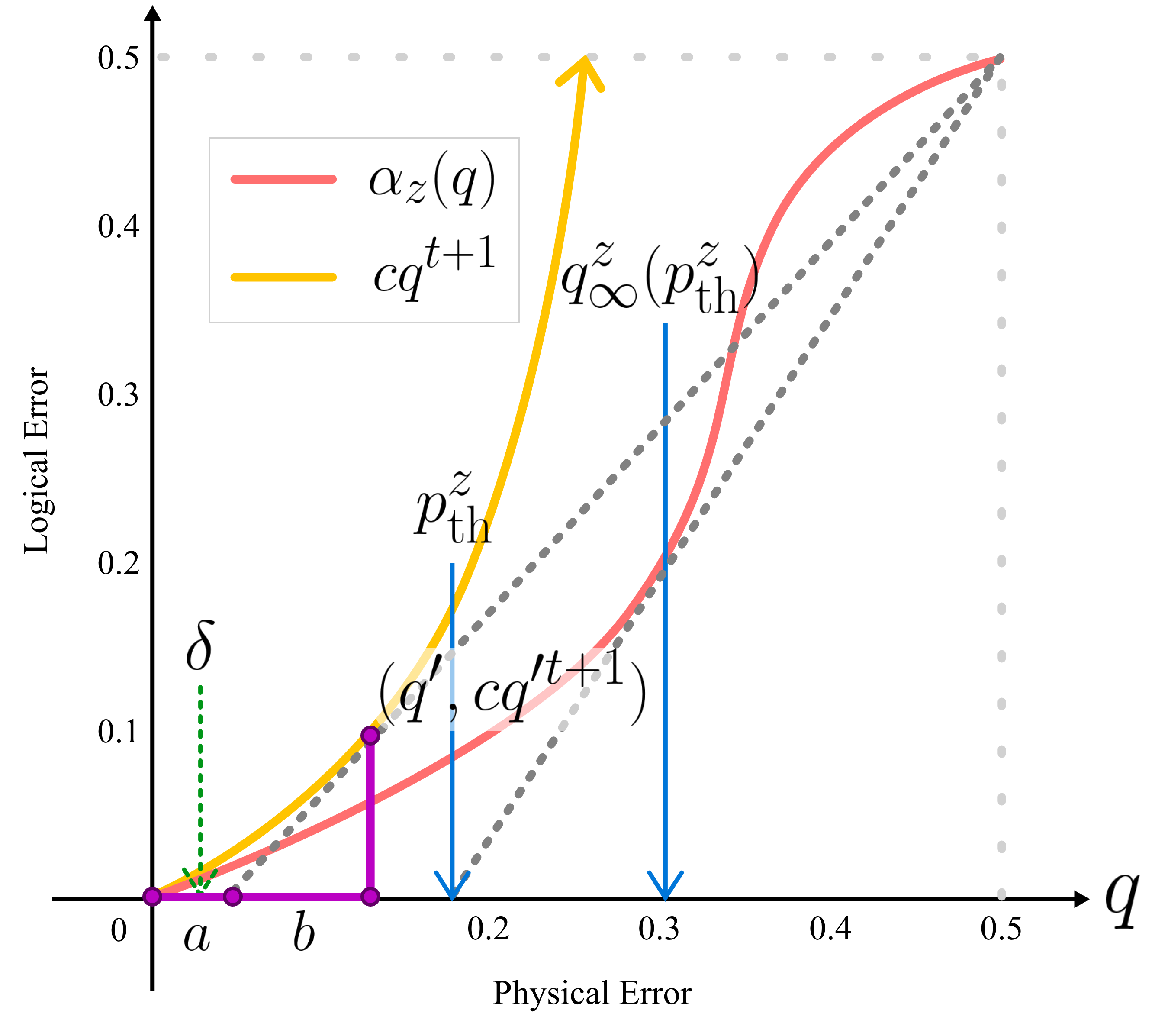
Figure 19: This plot illustrates the tangent line to $cq^{t_{z}+1}$ which passes through the point (0.5,0.5). The x-intercept of this line, denoted by $a$, is a lower bound on $p^{z}_{\rm th}$, i.e., $p^{z}_{\rm th}\geq a$. Suppose the tangent line intersects the curve $cq^{t_{z}+1}$ at point $(q^{\prime},cq^{\prime t_{z}+1})$. Define $b=q^{\prime}-a$. Because the slope of the tangent line at $q^{\prime}$ is equal to the derivative of curve $cq^{t_{z}+1}$ at this point, we find $\frac{cq^{\prime t_{z}+1}}{b}=(t_{z}+1)cq^{\prime t}_{z}$, which implies $b=\frac{q^{\prime}}{t_{z}+1}$, or equivalently, $a=\frac{t_{z}}{t_{z}+1}q^{\prime}.$ Finally, note that the slope of the tangent is greater than or equal to one, i.e., $(t_{z}+1)cq^{\prime t}_{z}\geq 1$, which means $q^{\prime}\geq\big{(}\frac{1}{(t_{z}+1)c}\big{)}^{{1}/{t_{z}}}$. We conclude that $a=\frac{t_{z}}{t_{z}+1}q^{\prime}\geq\frac{t_{z}}{t_{z}+1}\big{(}\frac{1}{(t_{z}+1)c}\big{)}^{{1}/{t_{z}}}$, which in turn implies $p^{z}_{\rm th}\geq a\geq\frac{t_{z}}{t_{z}+1}\big{(}\frac{1}{(t_{z}+1)c}\big{)}^{{1}/{t_{z}}}$. Thus, for $p_{z}\leq\delta$, the logical error upon local recovery of an infinite tree $q^{z}_{\infty}<1/2$, because $\delta\leq p^{z}_{\rm th}$.

C.1 Lower bound on $p^{z}_{\rm th}$

In the following, first we derive an upper bound on $\alpha$ and then as we describe in Fig. 19, based on this upper bound, we derive a lower bound on $p^{z}_{\rm th}$.

Suppose a CSS code corrects all $Z$ errors with weight less than or equal to $t_{z}$. Assuming each qubit is subjected to independent $Z$ error with probability $q$, then, after the error correction, the probability of $Z$ error is bounded by

$$\alpha_{z}(q)\leq\sum_{k=t_{z}+1}^{b}{b\choose k}q^{k}(1-q)^{b-k}\leq\Bigg{[}\sum_{k=t_{z}+1}^{b}{b\choose k}\Bigg{]}q^{t_{z}+1}\equiv cq^{t_{z}+1}\ ,$$ (136)

where $\sum_{k=t_{z}+1}^{b}{b\choose k}q^{k}(1-q)^{b-k}$ is the probability of $Z$ errors with weight $t_{z}+1$ or larger, and

$$c\equiv\sum_{k=t_{z}+1}^{b}{b\choose k}\leq 2^{b}\ .$$ (137)

As it can be seen from Fig. 19, since $cq^{t_{z}+1}\geq\alpha_{z}(q)$ for $q\in[0,0.5]$, the x-intercept of this line is smaller than or equal to the x-intercept of curve $\alpha_{z}(q)$ that passes through the point $(0.5,0.5)$. As we explain in the caption of Fig. 19, this implies that for

$$p_{z}\leq\frac{t_{z}}{t_{z}+1}\bigg{(}\frac{1}{(t_{z}+1)c}\bigg{)}^{\frac{1}{t_{z}}}\equiv\delta\ ,$$ (138)

$q^{z}_{\infty}$ is strictly less than $1/2$.

This proves the existence of a non-zero local recovery threshold for any CSS code tree with $d_{z}\geq 3$. Furthermore, this also lower bounds the optimal recovery threshold for $d_{z}\geq 3$ CSS code tree.

C.2 Upper bound on $q_{\infty}^{z}$

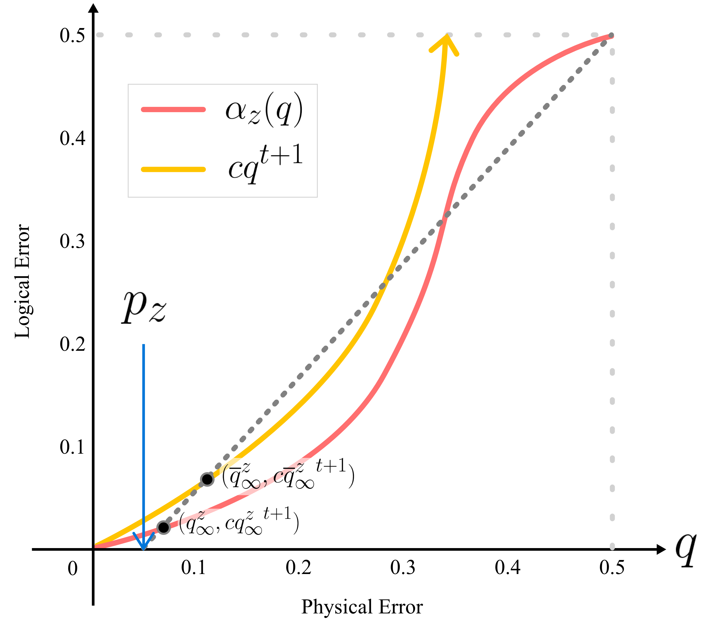
Figure 20: This figure illustrates how to estimate the logical error in an infinite CSS code tree after local recovery given that the $Z$ error within the tree is set at $p_{z}$. The line that passes through (0.5,0.5) and has $x$-intercept $p_{z}$ intersects $\alpha(q)$ at the point $(q^{z}_{\infty},\alpha(q^{z}_{\infty}))$. We show that the $q^{z}_{\infty}$ is the logical error in the infinite tree after local recovery. It is clear that $q^{z}_{\infty}$ depends on the specifics of $\alpha$, but we can upperbound $\alpha(q)\leq c\times q^{t_{z}+1}$, which allows an upperbound for $q^{z}_{\infty}$, which we denote by $\overline{q}^{z}_{\infty}$.

By definition, for $p_{z}<p^{z}_{\text{th}}$, we have $q_{\infty}^{z}<1/2$, which means after error correction the total error in the infinite tree is less than 1/2. In the following we establish an upper bound on $q_{\infty}^{z}$. We again use the fact that $\alpha(q)\leq cq^{t_{z}}$. As we saw above for sufficiently small $p_{z}$, e.g.,

$$p_{z}<\frac{t_{z}}{t_{z}+1}\bigg{(}\frac{1}{(t_{z}+1)c}\bigg{)}^{{1}/{t_{z}}}=\delta\ ,$$ (139)

the line $(q-p_{z})/(1-2p_{z})$ has two intersections with the curve $cq^{t_{z}+1}$. Let $(\overline{q},c\overline{q}^{t_{z}+1})$ be the coordinates of the intersection with smaller $x$ coordinates (see Fig. 20). More precisely $\overline{q}$ is the smallest positive real number satisfying

$$\frac{\overline{q}-p_{z}}{1-2p_{z}}=c\overline{q}^{t_{z}+1}\ .$$ (140)

At this point, the slope of the curve $cq^{t_{z}+1}$ is $(t_{z}+1)c\overline{q}^{t_{z}}$. Furthermore, because for $q$ in the interval $0<q<\overline{q}$, we have $\frac{q-p_{z}}{1-2p_{z}}<cq^{t_{z}+1}$, at the intersection the slope of line $(q-p_{z})/(1-2p_{z})$ is larger than the slope of the curve $cq^{t_{z}+1}$ (this can also be seen from Fig. ), that is,

$$(t_{z}+1)c\overline{q}^{t_{z}}\leq\frac{c\overline{q}^{t_{z}+1}}{\overline{q}-p_{z}}\ ,$$ (141)

where we have used the fact that the $x$-intercept of line $(q-p_{z})/(1-2p_{z})$ is $p_{z}$. Another way to justify this inequality is to notice that for point $q^{\prime}$ (as defined in Fig. 19),

$$(t_{z}+1)c{q^{\prime}}^{t_{z}}=\frac{c{q^{\prime}}^{t_{z}+1}}{{q^{\prime}}-a}.$$ (142)

Because $\overline{q}$ is the first point of intersection, we necessarily have that $\overline{q}<q^{\prime}$ and $a<p_{z}$. Thus,

$$(t_{z}+1)c\overline{q}^{t_{z}}\leq(t_{z}+1)c{q^{\prime}}^{t_{z}}=\frac{c{q^{\prime}}^{t_{z}+1}}{{q^{\prime}}-a}\leq\frac{c\overline{q}^{t_{z}+1}}{\overline{q}-p_{z}}.$$ (143)

We simplify Eq.(141) to,

$$\overline{q}\leq(1+\frac{1}{t_{z}}){p_{z}}\ .$$ (144)

Finally, we note that

$$q^{z}_{\infty}\leq\overline{q}\ ,$$ (145)

which can be seen from the Fig.20, or by noting that (i) $\overline{q}$ is the smallest positive real number satisfying Eq.(140), and (ii) $q^{z}_{\infty}$ is the smallest positive real number satisfying

$$\frac{q^{z}_{\infty}-p_{z}}{1-2p_{z}}=\alpha(q^{z}_{\infty})\ .$$ (146)

The latter means that for all $q$ in the interval $0<q<q^{z}_{\infty}$ it holds that

$$\frac{q-p_{z}}{1-2p_{z}}<\alpha(q)<cq^{t_{z}+1}\ ,$$ (147)

and, therefore, $\overline{q}$ is not in this interval. We conclude that

$$q^{z}_{\infty}\leq\overline{q}\leq(1+\frac{1}{t_{z}}){p_{z}}\ .$$ (148)

It is worth noting that if the code corrects single-qubit error, i.e., if $t_{z}\geq 1$, then for $q=1/2$ we have

$$c{\frac{1}{2^{t_{z}+1}}}>\alpha(\frac{1}{2})=\frac{1}{2}\ ,$$ (149)

which implies

$$c^{1/t_{z}}>2\ .$$ (150)

This implies that for

$$q^{z}_{\infty}\leq\overline{q}\leq(1+\frac{1}{t_{z}}){p_{z}}\leq(1+\frac{1}{t_{z}})\delta=\bigg{(}\frac{1}{(t_{z}+1)c}\bigg{)}^{{1}/{t_{z}}}<\frac{1}{2}\times\bigg{(}\frac{1}{t_{z}+1}\bigg{)}^{{1}/{t_{z}}}<\frac{1}{2}\ .$$ (151)

This gives another proof that for $p_{z}\leq\delta$, $q^{z}_{\infty}$ is strictly less than $1/2$.

C.3 Fixed-point equation for stabilizer codes with Pauli errors

Optimal recovery of a single block of stabilizer codes with Pauli errors can be realized by applying a Clifford unitary, measuring ancilla qubits in $\{|0\rangle,|1\rangle\}$ basis and performing a Pauli operator on the data qubit. It follows that if the noise channel $\mathcal{N}$ is a Pauli channel, then the sequence of channels defined by the recursive equation in Eq.(78) will be all Pauli channels. Then, as long as $\mathcal{N}_{\infty}$ is not the fully depolarizing channel $\mathcal{N}_{\infty}(\rho)=I/2$, it can transmit classical information. Also, for Pauli channels there are simple necessary and sufficient condition that determines whether the channel is entanglement-breaking, or not (see Appendix B.2).

Let $\textbf{q}=(q^{x},q^{y},q^{z})$ be the probability of $X$, $Y$, and $Z$ errors in channel $\mathcal{M}$ in Eq.(74). Then, the channel $f[\mathcal{M}]$ will be a Pauli channel in the form

$$f[\mathcal{M}](\rho)=\alpha_{I}(\textbf{q})\rho+\sum_{w=x,y,z}\alpha_{w}(\textbf{q})\ \sigma_{w}\rho\sigma_{w}\ ,$$ (152)

where $\alpha_{I}(\textbf{q})=1-\sum_{w=x,y,z}\alpha_{w}(\textbf{q})$. As is clear, if q is the probability of single-qubit error on the physical qubits, $\{\alpha_{w}(\textbf{q})\}_{w}$ is the probability of single-qubit error on the logical qubit. Let $\textbf{q}_{t}=({q}^{x}_{t},{q}^{y}_{t},{q}^{z}_{t})$ denote the error probabilities for the Pauli channel $\mathcal{N}_{t}$. Then, the recursive Eq.(78) can be rewritten as

$$\textbf{q}_{t+1} =\left(\alpha_{x}(\textbf{q}_{t}),\alpha_{y}(\textbf{q}_{t}),\alpha_{z}(\textbf{q}_{t})\right)\left(\begin{array}[]{ccc}p_{I}&p_{Z}&p_{Y}\\ p_{Z}&p_{I}&p_{X}\\ p_{Y}&p_{X}&p_{I}\end{array}\right)$$ (156)

$$+\big{[}1-\sum_{w=x,y,z}\alpha_{w}(\textbf{q}_{t})\big{]}(p_{X},p_{Y},p_{Z})\ ,$$ (157)

where $p_{X},p_{Y},p_{Z}$ are the error probabilities for channel $\mathcal{N}$, and $p_{I}=1-(p_{X}+p_{Y}+p_{Z})$.

Since the recovery $\mathcal{R}$ is a linear map, functions $\{\alpha_{w}(\textbf{q}):w=x,y,z\}$ are polynomials of, at most, degree $b$ in each variable $q^{x}$, $q^{y}$, and $q^{z}$. Furthermore, for codes with distance $d$, the recovery $\mathcal{R}$ can be chosen to correct all the errors with weight less than or equal to $\lfloor(d-1)/2\rfloor$. In this case, the lowest degree of monomials in $q^{x}$, $q^{y}$, and $q^{z}$ is $\lfloor(d-1)/2\rfloor+1$.

As we show in the following subsection, this implies that for codes with distance $d\geq 3$ there are positive error thresholds $p_{\text{th}}>p_{\text{ent}}>0$ such that for $p_{x},p_{y},p_{z}<p_{\text{th}}$ the channel $\mathcal{N}_{\infty}$ is not the fully depolarizing channel, hence transmitting (noisy) classical information, and for $p_{x},p_{y},p_{z}<p_{\text{ent}}$ the channel $\mathcal{N}_{\infty}$ is not entanglement-breaking, hence transmitting entanglement.

C.4 Non-zero noise threshold for general stabilizer code trees

Here, we show how the above argument can be generalized to the case of all stabilizer codes with Pauli errors. In particular, we show that if in Eq.(156) none of polynomials $\alpha_{x}$, $\alpha_{y}$ and $\alpha_{z}$ have linear terms, then there exists a positive threshold $p_{\text{th}}>0$ such that for $p_{x},p_{y},p_{z}<p_{\text{th}}$, Eq.(156) has fixed-point channels other than the fully depolarizing channel. To this end, we consider the probability of some error occurring $p=\sum_{w=x,y,z}p_{w}$, where $\mathbf{p}=(p_{x},p_{y},p_{z})$ is the probabilities associated to Pauli error. To study recovery, we define

$$\widetilde{\alpha}(p):=\sum_{p_{x}+p_{y}+p_{z}=p}\alpha(\mathbf{p}),$$

that is the probability of some logical error as a function of some physical error. Let $q_{t}$ indicate the probability of some error after local recovery of a tree of depth $t$. Then Eq.(156) can be turned into the inequality,

$$q_{t+1}\leq 1-(1-\widetilde{\alpha}(q_{t}))(1-p)$$ (158)

where we note the probability of no error in level $t+1$ is at least the probability of no error after recovery and no local error. We focus on the upperbound in Eq.(158) by defining $\epsilon_{t}$ as

$$\epsilon_{t+1}=1-(1-\widetilde{\alpha}(\epsilon_{t}))(1-p)$$

and $\epsilon_{0}=0$. These would satisfy $q_{t}\leq\epsilon_{t}$ for all $t$. The fixed point of this recursive relation for $\epsilon_{t}$, i.e., $\epsilon_{\infty}$, satisfies the equation,

$$\widetilde{\alpha}(\epsilon_{\infty})=\frac{\epsilon_{\infty}-p}{1-p}$$ (159)

It is clear that for stabilizer codes with distance $d\geq 3$, all errors with weight atmost $\widetilde{t}:=\lfloor(d-1)/2\rfloor$ will be corrected. Thus, $\tilde{\alpha}$ will have no terms of degree less than $\widetilde{t}+1$ in $q$ because it is a sum of $\alpha_{w}$’s which each do not have upto degree-$\widetilde{t}$ monomials. More specifically,

$$\widetilde{\alpha}(q)\leq\widetilde{c}\times q^{\widetilde{t}+1}$$ (160)

for positive constant $\widetilde{c}\geq 1$. Because it is an upperbound, the local recovery threshold estimate for $\widetilde{c}\times q^{\widetilde{t}+1}$ (denoted by $\widetilde{p}_{\rm th}$) will lowerbound the threshold estimate for $\widetilde{\alpha}(q)$, i.e., $\widetilde{p}_{\rm th}\leq{p}_{\rm th}$. Observe that the family of lines considered in the RHS of Eq.(159) are characterized as passing through $(1,1)$. Thus, the threshold is estimated by computing the $x$-intercept (i.e., $\widetilde{p}_{\rm th}$) of the line passing through $(1,1)$ that is tangent to $\widetilde{c}\times q^{\widetilde{t}+1}$. This is equivalent to the threshold computation for CSS codes detailed in Fig. 19 in Appendix C up to rescaling. That is, consider the two curves

$$y=\widetilde{c}\times q^{\widetilde{t}+1},\ {\rm and}\ y=\frac{q-\widetilde{p}_{\rm th}}{1-\widetilde{p}_{\rm th}},$$

where the latter is tangent to the former. Upon rescaling as $(q^{\prime},y^{\prime})=(q/2,y/2)$, the two curves become,

$$y^{\prime}=(\widetilde{c}2^{\widetilde{t}})\times{q^{\prime}}^{\widetilde{t}+1},\ {\rm and}\ y^{\prime}=\frac{q^{\prime}-2\widetilde{p}_{\rm th}}{1-2\widetilde{p}_{\rm th}},$$

where the latter remains tangent to the former. So, if we set $c=\widetilde{c}2^{\widetilde{t}}$ and note that the $x$-intercept is $2\widetilde{p}_{\rm th}$, we can invoke Eq.(91) to conclude,

$$2\widetilde{p}_{\text{th}}\geq\frac{\widetilde{t}}{\widetilde{t}+1}\bigg{(}\frac{1}{(\widetilde{t}+1)\widetilde{c}2^{\widetilde{t}}}\bigg{)}^{\frac{1}{\widetilde{t}}}.$$ (161)

Thus, noting that $\widetilde{p}_{\rm th}\leq p_{\rm th}$, we conclude the following extension of Proposition 5 to general stabilizer codes: consider a $d\geq 3$ stabilizer tree composed of a stabilizer code that can correct physical errors of weight upto $\widetilde{t}=\lfloor(d-1)/2\rfloor$, with noise on each edge with probability of some Pauli error being $p=p_{x}+p_{y}+p_{z}$. Then, for sufficiently small $p$, e.g.

$$p<\frac{1}{4}\frac{\widetilde{t}}{\widetilde{t}+1}\bigg{(}\frac{1}{(\widetilde{t}+1)\widetilde{c}}\bigg{)}^{\frac{1}{\widetilde{t}}},$$

the probability of some logical error in the $d\geq 3$ stabilizer tree of any depth $T$ upon local recovery, i.e. $q_{T}$, is upperbounded as,

$$q_{T}\leq p\times(1+\frac{1}{\widetilde{t}}).$$

This upperbounds the probability of some logical error in a $d\geq 3$ stabilizer tree because $q_{T}\leq q_{T}$ for all $T$.

Appendix D Examples – Computations for Local Recovery for specific stabilizer trees

D.1 Local Recovery threshold for classical trees

Consider the $\alpha_{cl}$ function for local recovery of classical trees. For simplicity, we shall focus on odd branching number. Then,

$$\alpha_{\rm maj}(p)=\sum_{k={{\lfloor b/2\rfloor}+1}}^{b}{b\choose k}p^{k}(1-p)^{b-k}=1-\sum_{k=0}^{\lfloor b/2\rfloor}{b\choose k}p^{k}(1-p)^{b-k}$$ (162)

As per this definition, $\alpha_{\rm maj}(0)=0$ and $\alpha_{\rm maj}(0.5)=0.5$ (the latter can be easily seen by noting that when $p=0.5$, the probability distribution is symmetric about $0-1$ exchange). From Sec. IV.2.1, we know that the x-intercept of the tangent to $\alpha_{cl}(p)$, that also passes through $(0.5,0.5)$, is $p_{\rm th}$. We prove that $\alpha_{\rm maj}(p)$ is convex, i.e. $\alpha^{\prime\prime}_{\rm maj}(p)\geq 0$ for $0\leq p\leq 0.5$ in Section D.1.1. Thus, the tangent to the $\alpha_{\rm maj}$ curve is the tangent line at $p=0.5$. Using the fact that the tangent must pass through $(0.5,0.5)$, we get that

$$p_{\rm th}=\frac{1}{2}\Big{(}1-\frac{1}{\alpha^{\prime}_{cl}(0.5)}\Big{)}.$$ (163)

We compute $\alpha^{\prime}_{\rm maj}(0.5)$ below:

$$\alpha^{\prime}_{\rm maj}(p)=-\sum_{k=0}^{\lfloor b/2\rfloor}{b\choose k}kp^{k-1}(1-p)^{b-k}+\sum_{k=0}^{\lfloor b/2\rfloor}{b\choose k}(b-k)p^{k}(1-p)^{b-k-1}$$ (164)

At $p=0.5$ this evaluates to,

$$\alpha^{\prime}_{\rm maj}(0.5)=2\sum_{k=0}^{\lfloor b/2\rfloor}\frac{1}{2^{b}}{b\choose k}(b-2k)$$ (165)

Notice that $\frac{1}{2^{b}}{b\choose k}$ is the binomial distribution in $k$ with $p=0.5$. Because we are considering the regime when $b\rightarrow\infty$, we use the normal approximation to the binomial distribution to get,

$$2\sum_{k=0}^{\lfloor b/2\rfloor}\frac{1}{2^{b}}{b\choose k}(b-2k) \approx-4\int_{0}^{k=b/2}\frac{1}{\sqrt{\pi b/2}}e^{-\frac{(k-b/2)^{2}}{b/2}}(k-b/2)dk\Bigg{(}1+\mathcal{O}\Big{(}\frac{1}{\sqrt{b}}\Big{)}\Bigg{)}$$ (166)

$$=-4\int_{-b/2}^{0}\frac{1}{\sqrt{\pi b/2}}e^{-\frac{x^{2}}{b/2}}xdx\Bigg{(}1+\mathcal{O}\Big{(}\frac{1}{\sqrt{b}}\Big{)}\Bigg{)}$$ (167)

where we did a change of variables as $x=k-b/2$ in the second equality. Because we are anyway in the regime where $b\rightarrow\infty$, we further approximate this as,

$$\approx-4\int_{-\infty}^{0}\frac{1}{\sqrt{\pi b/2}}e^{-\frac{x^{2}}{b/2}}xdx\Bigg{(}1+\mathcal{O}\Big{(}\frac{1}{\sqrt{b}}\Big{)}\Bigg{)}=\sqrt{\frac{2}{\pi}}\sqrt{b}\Bigg{(}1+\mathcal{O}\Big{(}\frac{1}{\sqrt{b}}\Big{)}\Bigg{)}=\sqrt{\frac{2}{\pi}}\Big{(}\sqrt{b}+\mathcal{O}(1)\Big{)}$$ (168)

By substituting this into Eq.(163), we get,

$$p_{th}=\frac{1}{2}\Bigg{(}1-\sqrt{\frac{\pi}{2}}\frac{1}{\sqrt{b}+\mathcal{O}(1)}\Bigg{)}=\frac{1}{2}\Bigg{(}1-\sqrt{\frac{\pi}{2}}\frac{1}{\sqrt{b}}\Bigg{)}+\mathcal{O}\Big{(}\frac{1}{b}\Big{)}$$ (169)

D.1.1 Convexity of $\alpha_{\rm maj}$

We start by rewriting $\alpha_{\rm maj}$ by noting that that the cumulative binomial distribution ${Pr}(X_{\rm bin}\leq k)$ can be written in terms of the regularized incomplete beta function $F(k;n,p)$ (refer to Eq.3.3 in Bryan and Wadsworth (1960)),

$$\alpha_{\rm maj}(p) =1-\sum^{\lfloor{b}/{2}\rfloor}_{k=0}{b\choose k}p^{k}(1-p)^{b-k}$$ (170)

$$=1-{\rm Pr}(X_{\rm bin}\leq\frac{b-1}{2})$$ (171)

$$=1-F(\frac{b-1}{2};b,p)$$ (172)

$$=1-\Big{[}\frac{b+1}{2}\Big{]}{b\choose\frac{b-1}{2}}\times\int_{0}^{1-p}t^{\frac{b-1}{2}}(1-t)^{\frac{b-1}{2}}dt$$ (173)

where $b$ is odd. Now we differentiate this expression twice with respect to $p$ rather easily,

$$\alpha^{\prime}_{\rm maj}(p) =\Big{[}\frac{b+1}{2}\Big{]}{b\choose\frac{b-1}{2}}\times(1-p)^{\frac{b-1}{2}}p^{\frac{b-1}{2}}$$ (174)

$$=\Big{[}\frac{b+1}{2}\Big{]}{b\choose\frac{b-1}{2}}\times(p-p^{2})^{\frac{b-1}{2}},$$ (175)

$$\alpha^{\prime\prime}_{\rm maj}(p) =\Big{[}\frac{b+1}{2}\Big{]}{b\choose\frac{b-1}{2}}\times\frac{b-1}{2}\times(p-p^{2})^{\frac{b-3}{2}}\times(1-2p).$$ (176)

Thus, $\alpha^{\prime\prime}_{\rm maj}(p)\geq 0$ for all $p\in[0,0.5]$.

D.2 Example: Local recovery threshold for Generalized Shor code

An important class of CSS codes are generalized Shor codes. The encoder of a Shor code of order $n$ is a serial concatenation of two repetition codes ($M_{1}$ and $M_{2}$) that are dual to each other, i.e., $M_{1}^{\otimes n}\circ M_{2}$, that are defined as

$$M_{1}\ket{c}=\ket{c}^{\otimes b}:\ \ \ \ c\in\{0,1\},$$ (177)

$$M_{2}=H^{\otimes n}\circ M_{1}\circ H,$$ (178)

where $H$ is the Hadamard gate. Observe that $M_{1}$ is the classical copier in the $Z$ basis, while $M_{2}$ is the same in the dual $X$ basis. Fig. 21 illustrates the encoder for $n=3$ that is the usual Shor-9 encoder, upto an additional Hadamard at the input to make it a standard encoder. We consider a two-step recovery of the generalized Shor code with two decoders for $M_{1}$ and $M_{2}$ respectively. These are majority voting procedures in the $Z$ and $X$ basis respectively. We denote them as $\mathcal{R}_{\rm maj}$ and $\mathcal{R}_{\rm par}:=\mathcal{H}\circ\mathcal{R}_{\rm maj}\circ\mathcal{H}^{\otimes n}$ respectively, where $\mathcal{H}(.)=H(.)H$.

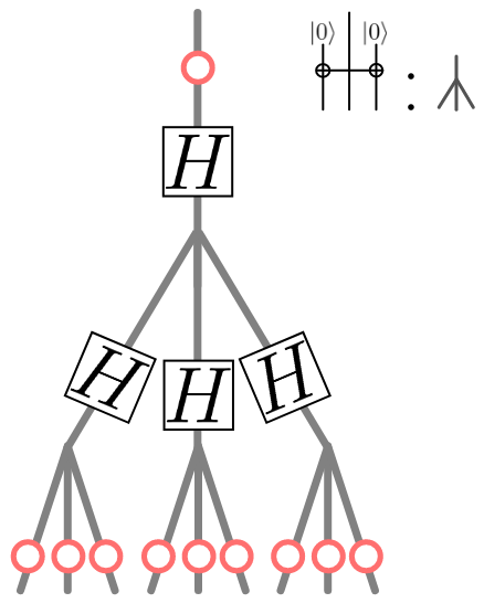
Figure 21: Encoder of a standard generalized Shor encoder with $n=3$– This the usual Shor-9 encoder. We have added a Hadamard gate to the root to ensure the encoder is standard with regards to $X$ and $Z$ logical operators.

We consider trees with a generalized Shor code encoder and independent single-qubit bit-flip and phase-flip errors, with probabilities $p_{x}$ and $p_{z}$ respectively, on each edge. Thus, the local recovery we apply to one level of the generalized Shor code is $\mathcal{R}_{\rm par}\circ\mathcal{R}_{\rm maj}^{\otimes n}$.

Define $\mathcal{M}_{i}(.)=M_{i}(.)M^{\dagger}_{i}$ for $i=1,2$. Notice that the evolution $X$ error in the channel $\mathcal{R}_{\rm maj}\circ\mathcal{N}^{\otimes n}_{x}\circ\mathcal{M}_{1}$ is $\alpha_{\rm maj}(p_{x})$ (defined in Eq.(93)) where $p_{x}$ is the probability of physical $X$ error. On the other hand, the evolution $X$ error in the channel $\mathcal{R}_{\rm par}\circ\mathcal{N}^{\otimes n}_{x}\circ\mathcal{M}_{2}$ is equivalent to the evolution of $Z$ error in the channel $\mathcal{R}_{\rm maj}\circ\mathcal{N}^{\otimes n}_{z}\circ\mathcal{M}_{1}$. Recall that a single-qubit physical $Z$ error is a logical error for the repetition code. So, logical error is determined by the parity of the weight of the physical error. Thus, the logical error rate associated with $\mathcal{R}_{\rm par}\circ\mathcal{N}^{\otimes n}_{x}\circ\mathcal{M}_{2}$ is

$$\alpha_{\rm par}(p_{x})=\frac{1}{2}-\frac{1}{2}(1-2p_{x})^{n}.$$ (179)

Thus, the evolution of $X$ error in the full channel

$$\mathcal{R}_{\rm par}\circ\mathcal{R}_{\rm maj}^{\otimes n}\circ\mathcal{N}^{\otimes n^{2}}_{x}\circ\mathcal{M}^{\otimes n}_{1}\circ\mathcal{M}_{2}$$

is

$$\alpha_{x}(p_{x})=\alpha_{\rm par}\circ\alpha_{\rm maj}(p_{x}).$$ (180)

It is easy to see that the above argument in the opposite order pertains to $Z$ errors. Thus,

$$\alpha_{z}(p_{z})=\alpha_{\rm maj}\circ\alpha_{\rm par}(p_{z}).$$ (181)

Using the procedure detailed in Sec. IV.2.1, we can numerically estimate the local recovery threshold $p_{\rm th}^{x}$ ($p_{\rm th}^{z}$) from $\alpha_{x}$ ($\alpha_{z}$) for all generalized Shor codes $[[n^{2},1,n]]$ as plotted in Fig. 22.

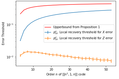
Figure 22: Noise threshold range for $[[n^{2},1,n]]$ Shor code tree for increasing $n$ – The upperbound $\frac{1}{2}(1-\frac{1}{\sqrt{n}})$ is obtained from Proposition 1. The local recovery thresholds, $p^{x}_{\rm th}$ and $p^{z}_{\rm th}$ (i.e., lowerbounds), are obtained from a numerical estimation procedure that benchmarks the local recovery strategy that is explained in Sec. IV.2.1. The upperbound is the same for both $X$ and $Z$ directions, while the lowerbounds are different and are indicated. With increasing $n$, while the $X$-error threshold improves, the $Z$-error threshold suffers. The $x$-axis indicates the order $n$ of $[[n^{2},1,n]]$ code for odd $n$, and the $y$-axis indicates the error threshold. The error bars of $0.001$ are determined by the resolution of the numerical estimation procedure.

Asymptotics for large $n$ – When we study the asymptotic case of large $n$, we majority voting is equivalent to an asymptotic binomial hypothesis testing scenario for which we can use the exponential Chernoff’s bound, that is,

$$\alpha_{\rm maj}(p_{x})\lesssim e^{-\frac{n}{3}(\frac{1}{2}-p_{x})}.$$

This gives us that

$$\alpha_{x}(p_{x})\lesssim\frac{1-(1-2e^{-\frac{n}{3}(\frac{1}{2}-p_{x})})^{n}}{2},$$

which clearly goes to $0$ for large $n$. This shows that for large $n$, we have $p^{z}_{\rm th}\rightarrow 1/2$ because the error goes to zero.

When we study the large-$n$ asymptotics for $\alpha_{z}(p_{z})$, observe that $\alpha_{\rm par}(p_{z})=\frac{1}{2}-\frac{(1-2p_{z})^{n}}{2}\rightarrow\frac{1}{2}$ as $n\rightarrow\infty$. Thus, $\alpha_{z}(p_{z})\rightarrow 1/2$ for large $n$. This implies that $p^{z}_{\rm th}\rightarrow 0$, i.e., an absence of a non-trivial local recovery threshold asymptotically.

Asymmetry in $X$ and $Z$ performance – The worse performance of recovery for $X$-direction information as compared to $Z$-direction information is a consequence of the asymmetry in the number of $Z$-type and $X$-type stabilizers in the Shor code’s stabilizer generators. Consider the $[[n^{2},1,n]]$ code of order $n$. We then have $n(n-1)$ $Z$-type stabilizer generators, and $(n-1)$ $X$-type stabilizer generators. Thus, there are $n$ times more $Z$-type stabilizer generators than $X$-type stabilizer generators. This entails a much greater sensitivity to detect and correct $X$ errors (using $Z$-type stabilizers) than $Z$ errors. Furthermore, this discrepancy increases with increasing $n$. This reflects as lower local recovery thresholds for $X$-direction as compared to $Z$-direction, seen in Fig. 22.

D.3 Probability of logical error for CSS codes

When studying distinguishability in (say) the $Z$ direction, recall that it suffices to consider the dephased version of a CSS code. Thus, the $\alpha$ function for a CSS code can be computed by considering the bit-flip error before and after classical local recovery of the associated dephased encoder.

To estimate the performance of local recovery for such CSS codes, we compute the total variation distance (TVD) between the distributions we obtain, for input 0 and 1, from the dephased tree classical encoder, followed by bit-flip noise. This TVD expression allows us to compute the $\alpha$ for the said CSS code, because the error after optimal recovery of a single level, i.e., $\alpha$, is $(1-{\rm TVD})/2$.

To estimate the $\alpha$ function, we shall first compute the total variation distance (TVD) between the output distribution of our $Z$-dephased CSS encoders along with local bit-flip noise of probability $p$. This is because the optimum Helstrom measurement will achieve the least error probability $\alpha(p)=(1-{\rm TVD(p)})/2$. Firstly, we indicate the distributions we obtain given input $0$ and $1$, in density matrix notation, as a convex mixture,

$$\rho_{0} =\frac{1}{|C_{2}|}\sum_{x\in C_{2}}|{x}\rangle\!\langle x|$$ (182)

$$\rho_{1} =\frac{1}{|C_{2}|}\sum_{x\in C_{2}}|{x+\mathbf{x}_{L}}\rangle\!\langle x+\mathbf{x}_{L}|$$ (183)

where $\mathbf{x}_{L}$ is the bitstring form of $X_{L}$ operator. At this point, these two states are fully distinguishable. Now we apply local bit-flip noise $\mathcal{N}_{p}(\rho)=(1-p)\rho+pX\rho X$, on the above two states and measure their distinguishability. That is, we compute,

$${\rm TVD}(p)=||\mathcal{N}_{p}^{\otimes n}(\rho_{0})-\mathcal{N}_{p}^{\otimes n}(\rho_{1})||_{1}$$ (184)

We compute one of these states,

$$\mathcal{N}_{p}^{\otimes n}(\rho_{0})$$ (186)

$$= \frac{1}{|C_{2}|}\sum_{x\in C_{2}}\sum_{y\in\{0,1\}^{n}}p^{|y|}(1-p)^{n-|y|}|{x+y}\rangle\!\langle x+y|$$ (187)

$$= \frac{1}{|C_{2}|}\sum_{x,y\in\{0,1\}^{n}}p^{|y|}(1-p)^{n-|y|}\delta(x\in C_{2})|{x+y}\rangle\!\langle x+y|$$ (188)

$$= \frac{1}{|C_{2}|}\sum_{z\in\{0,1\}^{n}}\Big{(}\sum_{y\in\{0,1\}^{n}}p^{|y|}(1-p)^{n-|y|}\delta(z-y\in C_{2})\Big{)}|{z}\rangle\!\langle z|$$ (189)

where in the last step we simply changed variables. Now, $\delta(z-y\in C_{2})$ is the restriction that $z$ and $y$ belong to the same additive coset of $C_{2}$ in $\{0,1\}^{n}$. We shall indicate that coset by $[C_{2}+z]$ for a given $z$. Thus, we can re-write the above expression as,

$$=\frac{1}{|C_{2}|}\sum_{z\in\{0,1\}^{n}}\Big{(}\sum_{y\in[C_{2}+z]}p^{|y|}(1-p)^{n-|y|}\Big{)}|{z}\rangle\!\langle z|$$ (190)

Define $\sigma_{p}([C_{2}+z]):=\sum_{y\in[C_{2}+z]}p^{|y|}(1-p)^{n-|y|}$, which is a non-negative number associated to each additive coset of $C_{2}$. This gives,

$$\rho_{0}=\frac{1}{|C_{2}|}\sum_{z\in\{0,1\}^{n}}\sigma_{p}([C_{2}+z])\ |{z}\rangle\!\langle z|$$ (191)

We obtain $\rho_{1}$ by noticing that the distribution is $\rho_{0}$ plus a shift by $\mathbf{x}_{L}$.

$$\rho_{1}=\frac{1}{|C_{2}|}\sum_{z\in\{0,1\}^{n}}\sigma_{p}([C_{2}+z+\mathbf{x}_{L}])\ |{z}\rangle\!\langle z|$$ (192)

Thus, we have,

$$||\mathcal{N}_{p}^{\otimes n}(\rho_{0})-\mathcal{N}_{p}^{\otimes n}(\rho_{1})||_{1}$$ (193)

$$= \frac{1}{2|C_{2}|}\sum_{z\in\{0,1\}^{n}}|\sigma_{p}([C_{2}+z])-\sigma_{p}([C_{2}+z+\mathbf{x}_{L}])|.$$ (194)

We shall refine our notation to highlight only the important objects. Let $\mathcal{C}$ indicate the set of cosets of $C_{2}$ in $\{0,1\}^{n}$, and $K\in\mathcal{C}$ is a member of that set, i.e., a specific coset. Define,

$$\sigma_{p}(K)=\sum_{y\in K}p^{|y|}(1-p)^{n-|y|},$$

where the summation is over all bitstrings belonging to coset $K$. Noticing that $\sigma_{p}(.)$ is defined for entire cosets, we partition our $z$ summation in terms of cosets and sum over these cosets and see that,

$$||\mathcal{N}_{p}^{\otimes n}(\rho_{0})-\mathcal{N}_{p}^{\otimes n}(\rho_{1})||_{1}$$ (195)

$$= \frac{1}{2|C_{2}|}\sum_{K\in\mathcal{C}}|C_{2}|\cdot|\sigma_{p}(K)-\sigma_{p}(K+\mathbf{x}_{L})|,$$ (196)

where we used the fact that every additive coset of $C_{2}$ has the same size $|C_{2}|$. So, in terms of cosets $K\in\mathcal{C}$, we have,

$$||\mathcal{N}_{p}^{\otimes n}(\rho_{0})-\mathcal{N}_{p}^{\otimes n}(\rho_{1})||_{1}=\frac{1}{2}\sum_{K\in\mathcal{C}}|\sigma_{p}(K)-\sigma_{p}(K+\mathbf{x}_{L})|,$$ (197)

where $\sigma_{p}(K)$ is understood as the probability that any bitstring in the coset $K$ is sampled by the bit-flip noise process with bit-flip probability $p$. For the Helstrom bound saturating measurement, the probability of error is (1-TVD)/2, which is the $\alpha$ value. Thus,

$$\alpha(p)=\frac{1}{2}-\frac{1}{4}\sum_{K\in\mathcal{C}}|\sigma_{p}(K)-\sigma_{p}(K+\mathbf{x}_{L})|.$$

An important special case are CSS codes for whom $X^{\otimes b}$ is a logical $Z$ operator, i.e., $\mathbf{x}_{L}=1^{\otimes b}\equiv\overline{1}$. In that case,

$$\alpha(p)=\frac{1}{2}-\frac{1}{4}\sum_{K\in\mathcal{C}}|\sigma_{p}(K)-\sigma_{p}(K+\overline{1})|=\frac{1}{2}-\frac{1}{4}\sum_{K\in\mathcal{C}}|\sigma_{p}(K)-\sigma_{1-p}(K)|.$$

D.4 Steane-7 Code Coset structure and $\alpha$ function

Computing $\sigma_{p}$ for different cosets comes down to knowing the distribution of weights in the different cosets. We know this weight distribution exactly for the Steane-7 code. We explicitly compute this in the following.

The $C_{2}$ for the Steane-7 Code corresponds to the dual of the $[7,4,3]$ Hamming code that is used to construct the Steane-7 code. We see that the 3 generators of $C_{2}$ in $\mathbb{Z}_{2}^{7}$ are,

$\begin{pmatrix}1&0&1&0&1&0&1\\ 0&1&1&0&0&1&1\\ 0&0&0&1&1&1&1\end{pmatrix}$

When we look at the $2^{3}=8$ vectors generated by these generators, we get,

$\begin{pmatrix}0&0&0&0&0&0&0\\ 1&0&1&0&1&0&1\\ 0&1&1&0&0&1&1\\ 0&0&0&1&1&1&1\\ 0&1&1&1&1&0&0\\ 1&1&0&0&1&1&0\\ 1&0&1&1&0&1&0\\ 1&1&0&1&0&0&1\\ \end{pmatrix}$

We see the weight distribution of $C_{2}$ is $(0,4,4,4,4,4,4,4)$, where each component is the weight of one of the eight elements. Next, we have $2^{7}/2^{3}-1=2^{4}-1=15$ cosets of $C_{2}$. One coset is simply the complement of $C_{2}$, i.e., $C_{2}+\overline{1}$, with the weights $(7,3,3,3,3,3,3)$. We can compute $7$ other cosets by adding vectors like $(1,0,0,0,0,0,0)$, $(0,1,0,0,0,0,0)$, and so on to the $8$ vectors in $C_{2}$. Adding such a unit vector to any vector can only change the weight by $\pm 1$. Additionally observe that each column has exactly four $1$’s. Thus, adding a unit vector will ensure the total weight remains the same. Thus, the weights are $(1,3,3,3,3,5,5,5)$. The remaining $7$ cosets are the complement of the above mentioned $7$; Thus, have weight distribution $(6,4,4,4,4,2,2,2)$. We can use this to compute $\sigma_{p}(K)$ for each coset as a function of $p$, and thus, its $\alpha$ function which is,

$$\alpha_{\rm Steane-7}(p)=21p^{2}-98p^{3}+210p^{4}-252p^{5}+168p^{6}-48p^{7}.$$ (198)

Appendix E $d=2$ code tree error analysis

E.1 Derivation of Proposition 6

In this section, we present an error analysis for the recursive decoder introduced in Sec.V.1 and prove proposition 6. Recall that in this proposition we focus on codes with distance $d=2$. In the statement of the proposition, we denote the total probability of error in the Pauli channel $\mathcal{N}$ by $p_{\text{tot}}=p_{x}+p_{y}+p_{z}$. For convenience, in this section, we use the more compact notation $p$ for $p_{\text{tot}}$.

Consider the decoding between level $t-1$ and $t$ (see Fig 11). The decoder module (detailed in Sec.(V.1)) acts on $b$ qubits along with their reliability bits $\{m_{i}(t-1)\}_{i\in[b]}$. We refer to these $b$ input qubits as the block. The output of the decoder is a single qubit along with its reliability bit $m(t)$. We define a bit $e(t)$, which takes value $e(t)=1$ when the output qubit has no error, and $e(t)=1$ if it does. In other words, $e(t)$ indicates whether there is a logical error after recursive decoding of $t$ levels. Thus, we can define the probabilities,

$${\text{Probability of a qubit being marked: }}\mu_{t} ={\rm Pr}(m(t)=1),$$ (199)

$${\text{Probability of an unmarked error: }}\delta_{t} ={\rm Pr}(e(t)=1\ {\rm and}\ m(t)=0).$$ (200)

Note that these probabilities are identical for all the blocks at the same level. We show in Sec. E.2 that these probabilities satisfy the coupled recursive relations

$$\mu_{t} \leq b(\delta_{t-1}+p)+b^{2}\mu_{t-1}(\delta_{t-1}+p)+b^{2}\mu^{2}_{t-1}$$ (201)

and

$$\delta_{t} \leq b^{2}(\delta_{t-1}+p)^{2}+b^{2}\mu_{t-1}(\delta_{t-1}+p)\ ,$$ (202)

with the initial conditions $\mu_{0}=0$ and $\delta_{0}=0$. Recursive application of these coupled equations allows us to upperbound the error after $t$ rounds of recursive decoding. We show in Sec E.3 that when $p<1/\lambda\equiv 1/(16b^{4}+4b^{2})$, these quantities satisfy

$$\mu_{t} \leq 4b^{2}\times(p+\lambda p^{2})\leq 8b^{2}p,$$ (203)

$$\delta_{t} \leq\lambda p^{2}.$$ (204)

for all $t$. For the second upperbound for $\mu_{t}$ we simply notice that for $p<1/\lambda$, we have $p\lambda<1$.

Ignoring the reliability bit and just focusing on the total probability of logical error, one finds

$${\rm Pr}(e(t)=1) ={\rm Pr}(e(t)=1\ {\rm and}\ m(t)=0)+{\rm Pr}(e(t)=1|m(t)=1)\times{\rm Pr}(m(t)=1)$$

$$\leq\delta_{t}+\mu_{t},$$

where we have applied Bayes’ rule. Combining this with the tighter bounds above we conclude that for all $t$,

$${\rm Pr}(e(t)=1) \leq 4b^{2}p+(1+4b^{2})\times\lambda p^{2}$$ (205)

$$\leq(1+8b^{2})\times p$$ (206)

when $p<1/\lambda\equiv 1/(16b^{4}+4b^{2})$. In the second line we used that $p\lambda<1$. This proves Proposition 6.

E.2 Derivation of recursive relations Eq.(201) and Eq.(202)

Figure 23: This figure illustrates the recovery of a single block at level $t$ during recursion. In this figure, let $\mathcal{N}_{t-1}$ denote the effective Pauli channel we obtain after recursive decoding of $t-1$ levels. The output of $\mathcal{N}_{t-1}$ is the qubit after $t-1$ levels of recovery along with its reliability bit $m_{i}(t-1)$, indexed $i$. A total of $b$ such channels, along with the physical error in the encoder (indicated as the small unlabeled red dots) form the input for the decoder $\mathcal{R}_{\rm d=2}$ at level $t$ of recovery.

In this section, we prove the recursive relations. Since all blocks of $b$ qubits in level $t$ (or $t-1$) are identical. So we focus on the update of one particular block.

We make some remarks regarding the error probabilities within a block: Consider a block of $b$ qubits received by the decoder module at level $t$ (see Fig.11). From the point of this decoder, each qubit may contain unmarked errors, caused by the following two random independent processes: (i) unmarked error in the output of the decoder at level $t-1$, which has probability $\delta_{t-1}$ or (ii) the physical error in the encoder at level $t$, which has probability $p$ (see Fig. 23). Then, union bound implies that the probability of an unmarked error on each input qubit received by the decoder module is, at most, $\delta_{t-1}+p$. Thanks to the tree structure, the event of the $i^{\rm th}$ qubit being marked (or containing unmarked errors) is independent of similar events for $j^{\rm th}$ qubit. Finally, when we say a detected error, it means that the error produced a non-zero syndrome. We also repeatedly use the very useful bound $(1-x)^{n}\geq 1-nx$ when $0\leq x\leq 1$ and $b\geq 1$.

Derivation of Eq.(201)

Now we derive the bound for $\mu_{t}={\rm Pr}(m(t)=1)$. We note that if there is only one marked qubit and none of the other qubits contain errors, either no syndrome will be observed, or the observed syndrome will be consistent with the marked qubit. In both cases, the algorithm sets $m(t)=0$. Therefore, the events that cause sending a message to the next level, i.e., set $m(t)=1$ are a subset of the union of the following events:

• (A) No qubit is marked and, at least, one of the qubits contains an error, which happens with probability bounded by $1-(1-[p+\delta_{t-1}])^{b}\leq b\times[p+\delta_{t-1}]$.

• (B) More than one qubit is marked, which happens with probability bounded by

  $$1-b\mu_{t-1}(1-\mu_{t-1})^{b-1}-(1-\mu_{t-1})^{b} =1-(1-\mu_{t-1})^{b-1}[1+(b-1)\mu_{t-1}]$$ (207a)

  $$\leq 1-(1-(b-1)\mu_{t-1})(1+(b-1)\mu_{t-1})$$ (207b)

  $$=(b-1)^{2}\times\mu_{t-1}^{2}\ ,$$ (207c)

  where to get the second line we have used $(1-x)^{b-1}\geq 1-(b-1)x$.

• (C) A qubit is marked and other unmarked qubits contain errors. To find this probability, consider the special case in which qubit $r=1$ is marked whereas qubits $2,\cdots,b$ are unmarked and contain errors. The probability of this event is bounded by $\mu_{t-1}\times(b-1)\times(p+\delta_{t-1})$. This joint probability is the same for all other configurations $r=2,\cdots,b$. Therefore, the total probability of event C is bounded by $b(b-1)\times\mu_{t-1}\times(p+\delta_{t-1})$.

Therefore, applying the union bound we find

$$\mu_{t}=\text{Pr}(m(t)=1)\leq\text{Pr}(A\cup B\cup C) \leq\text{Pr}(A)+\text{Pr}(B)+\text{Pr}(C)$$ (208)

$$\leq b[\delta_{t-1}+p]+(b-1)^{2}\times\mu^{2}_{t-1}+b(b-1)\times\mu_{t-1}\times(p+\delta_{t-1})\ .$$ (209)

Eq.(201) is a weaker version of this bound, obtained by replacing $b-1$ with $b$.

Derivation of Eq.(202)

Next, we derive the bound for $\delta_{t}={\rm Pr}(e(t)=1\ {\rm and}\ m(t)=0)$. Recall that the event where the algorithm sets $m(t)=0$ and yet $e(t)=1$ are subsets of the following events: (C) a qubit is marked and other unmarked qubits contain errors. (D) no syndrome is observed, i.e., $\textbf{s}=\textbf{0}$, and none of the qubits is marked and yet there is an error. We bound the probability of each event separately.

• (C) See above.

• (D) Since the code has distance $d=2$, it detects single-qubit errors. Therefore, to have an error $e(t)=1$ without observing any syndrome ($\textbf{s}=\bf{0}$), there should be, at least, two errors. The probability that a qubit is unmarked and contains an error is bounded by $p+\delta_{t-1}$. Therefore, the probability of this event is bounded by

  $$1-b[\delta_{t-1}+p](1-[\delta_{t-1}+p])^{b-1}-(1-[\delta_{t-1}+p])^{b}\leq(b-1)^{2}\times(\delta_{t-1}+p)^{2}\ ,$$ (210)

  where the derivation is similar to Eq.(207).

Then, applying the union bound we find

$$\delta_{t}={\rm Pr}(e(t)=1\ {\rm and}\ m(t)=0)\leq\text{Pr}(C\cup D)\leq\text{Pr}(C)+\text{Pr}(D)\leq(b-1)^{2}\times(\delta_{t-1}+p)^{2}+b(b-1)\times\mu_{t-1}(p+\delta_{t-1})\ .$$ (211)

Eq.(202) is a weaker version of this bound, obtained by replacing $b-1$ with $b$.

E.3 Analysis of recursive relations Eq.(201) and Eq.(202)

Here, we analyze the recursive relations Eq.(201) and Eq.(202), namely

$$\mu_{t} \leq b(\delta_{t-1}+p)+b^{2}\mu_{t-1}(\delta_{t-1}+p)+b^{2}\mu^{2}_{t-1}\ ,$$

$$\delta_{t} \leq b^{2}(\delta_{t-1}+p)^{2}+b^{2}\mu_{t-1}(\delta_{t-1}+p)\ .$$

In particular, the goal is to find upper bounds on $\mu_{t}$ and $\delta_{t}$ that hold for arbitrary large $t$. To simplify these equations, we substitute $\epsilon_{t}=\delta_{t}+p$ to obtain,

$$\mu_{t} \leq b\epsilon_{t-1}+b^{2}\mu_{t-1}\epsilon_{t-1}+b^{2}\mu^{2}_{t-1},$$ (212)

$$\epsilon_{t} \leq p+b^{2}\epsilon_{t-1}^{2}+b^{2}\mu_{t-1}\epsilon_{t-1}.$$ (213)

Also, for convenience, in the following we use the slightly weaker bounds

$$\mu_{t} \leq 2b^{2}\epsilon_{t-1}+b^{2}\mu^{2}_{t-1}=f(\mu_{t-1},\epsilon_{t-1}),$$ (214a)

$$\epsilon_{t} \leq p+b^{2}\epsilon_{t-1}^{2}+b^{2}\mu_{t-1}\epsilon_{t-1}=g(\mu_{t-1},\epsilon_{t-1})\ \ ,$$ (214b)

where we have applied condition $\mu_{t}\leq 1$, and defined

$$f(x,y) :=b^{2}x^{2}+2b^{2}y\ ,$$ (215)

$$g(x,y) :=p+b^{2}y^{2}+b^{2}xy\ .$$ (216)

To understand the behavior of these recursive inequalities we focus on the following recursive equalities

$$x_{t} =f(x_{t-1},y_{t-1})=2b^{2}y_{t-1}+b^{2}x^{2}_{t-1}\ ,$$ (217a)

$$y_{t} =g(x_{t-1},y_{t-1})=p+b^{2}y^{2}_{t-1}+b^{2}x_{t-1}y_{t-1}\ ,$$ (217b)

with the initial condition

$$x_{0}=\mu_{0}=0\ ,\ \ \ y_{0}=\epsilon_{0}=p>0\ .$$ (218)

We note that because for $x,y\geq 0$ functions $f$ and $g$ are monotone in both variables, then applying bounds in Eq.(214a) recursively imply that

$$\mu_{t}\leq x_{t}\ ,\ \ \epsilon_{t}\leq y_{t}\ .$$ (219)

Suppose $x_{\infty},y_{\infty}>0$ are a fixed point of Eq.(217), i.e., they satisfy

$$x_{\infty} =f(x_{\infty},y_{\infty})=2b^{2}y_{\infty}+b^{2}x^{2}_{\infty},$$ (220)

and

$$y_{\infty} =g(x_{\infty},y_{\infty})=p+b^{2}y^{2}_{\infty}+b^{2}x_{\infty}y_{\infty}\ .$$ (221)

Then, again the monotonicity of functions $f$ and $g$ imply that if $x_{0}\leq x_{\infty}$ and $y_{0}\leq y_{\infty}$, then $x_{t}\leq x_{\infty}$ and $y_{t}\leq y_{\infty}$ for all $t$, i.e.,

$$x_{t} =f(x_{t-1},y_{t-1})\leq f(x_{\infty},y_{\infty})=x_{\infty},$$ (222)

$$y_{t} =g(x_{t-1},y_{t-1})\leq g(x_{\infty},y_{\infty})=y_{\infty}\ .$$ (223)

Therefore, if the initial condition in Eq.(218) satisfy the constraint $y_{0}=\epsilon_{0}=p\leq y_{\infty}$, it is guaranteed that for all $t$,

$$\epsilon_{t} \leq y_{t}\leq y_{\infty}\ ,$$ (224)

$$\mu_{t} \leq x_{t}\leq x_{\infty}\ .$$ (225)

In the following, we show that for $p<1/(16b^{4}+4b^{2})$, there is a fixed point solution that satisfies

$$2b^{2}p\leq \ x_{\infty}\leq 4b^{2}p+4b^{2}(16b^{4}+4b^{2})p^{2},$$ (226)

$$p\leq \ y_{\infty}\leq p+(16b^{4}+4b^{2})p^{2}.$$ (227)

The initial conditions, $x_{0}=0$ and $y_{0}=p$, clearly satisfy $x_{0}\leq x_{\infty}$ and $y_{0}\leq y_{\infty}$. So we conclude that $x_{t}\leq x_{\infty}$ and $y_{t}\leq y_{\infty}$ for all $t$ (this also justifies the use of the subscript $\infty$). Recalling that these were upperbounds, we get that when $p<1/(16b^{4}+4b^{2})$,

$$\mu_{t} \leq 4b^{2}p+4b^{2}(16b^{4}+4b^{2})p^{2},$$ (228)

$$\epsilon_{t} \leq p+(16b^{4}+4b^{2})p^{2}.$$ (229)

for all $t$. Undoing the substitution $\epsilon_{t}=\delta_{t}+p$, we conclude that when $p<1/\lambda\equiv 1/(16b^{4}+4b^{2})$,

$$\mu_{t} \leq 4b^{2}\times(p+\lambda p^{2}),$$ (230)

$$\delta_{t} \leq\lambda p^{2}.$$ (231)

for all $t$.

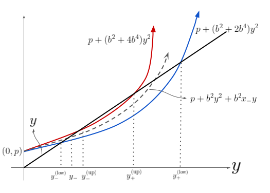
Figure 24: Schematic for intersection of the line $y$ (black) with the functions $p+(b^{2}+2b^{4})y^{2}$ (blue), $p+b^{2}y^{2}+b^{2}x_{-}y$ (dashed), and $p+(b^{2}+4b^{4})y^{2}$ (red).

E.3.1 $x_{\infty}$ and $y_{\infty}$ computation

Now we compute a specific solution for $x_{\infty}$ and $y_{\infty}$ that satisfies Eq.(220) and Eq.(221). We drop the $\infty$ subscript for clarity. Note that in general, these two equations will have 4 solutions. It suffices to estimate one real non-negative solution. We first solve Eq.(220) for $x$ to get,

$$x_{\pm}=\frac{1\pm\sqrt{1-8b^{4}y}}{2b^{2}}$$ (232)

For real solutions, we require $y<1/8b^{4}$. Then using the useful bounds

$$1-a\leq\sqrt{1-a}\leq 1-a/2\ \ {\rm when}\ 0\leq a\leq 1,$$ (233)

we get that the two solutions are bounded as,

$$2b^{2}y\leq \ x_{-}\leq 4b^{2}y,$$ (234)

$$\frac{1-4b^{4}y}{b^{2}}\leq \ x_{+}\leq\frac{1-2b^{4}y}{b^{2}}.$$ (235)

Observe that the ’+’ solution predicts that if $y=0$, then $x=1/b^{2}$. Whereas the ‘-’ predicts that if $y=0$, then $x=0$. We argued earlier that any non-negative set of fixed points would provide a valid upperbound. So, we may as well choose the tighter upperbound, i.e., the ‘-’ solution. Now we solve Eq.(221) after substituting $x_{-}$ in it. Using the bounds for $x_{-}$, we get that the RHS of Eq.(221) is bounded as

$$p+(b^{2}+2b^{4})y^{2}\leq p+b^{2}y^{2}+b^{2}x_{-}y\leq p+(b^{2}+4b^{4})y^{2}.$$ (236)

Eq.(221) is guaranteed a solution if the line $y$ intersects the upperbound $p+(b^{2}+4b^{4})y^{2}$. So, we are guaranteed an intersection (i.e., a solution) when $p<1/(16b^{4}+4b^{2})$.

Now we study these solutions fixing such a $p<1/(16b^{4}+4b^{2})$. Observe that the lower and upper bounds are convex parabolas that pass through $(0,p)$. So the line $y$ will intersect each parabola twice. We shall label the solutions for the lower parabola $y^{\rm(low)}_{\pm}$ and the solutions for the upper parabola $y^{\rm(up)}_{\pm}$ (Fig. (24) clarifies this). Observe that there will be an intersection between the line $y$ and $p+b^{2}y^{2}+b^{2}x_{-}y$ (that we denote by $y_{-}$) between $y^{\rm(low)}_{-}$ and $y^{\rm(up)}_{-}$. Now we estimate these two:

$$y^{\rm(up)}_{-} =\frac{1-\sqrt{1-(16b^{4}+4b^{2})p}}{8b^{4}+2b^{2}}\leq p+(16b^{4}+4b^{2})p^{2}$$ (237)

$$y^{\rm(low)}_{-} =\frac{1-\sqrt{1-(8b^{4}+4b^{2})p}}{4b^{4}+2b^{2}}\geq p.$$ (238)

Thus, we have $p\leq y_{-}\leq p+(16b^{4}+4b^{2})p^{2}$ when $p<1/(16b^{4}+4b^{2})$. Now we take this value of $y_{-}$ and substitute it back into Eq.(232) to compute $x_{-}$. From the bounds we saw for $x_{-}$, we conclude that $x_{-}\leq 4b^{2}y_{-}\leq 4b^{2}p+4b^{2}(16b^{4}+4b^{2})p^{2}$ and $x_{-}\geq 2b^{2}y_{-}\geq 2b^{2}p$. Furthermore, for the regime of $p$ we are considering, this upperbound for $y_{-}$ (i.e., $2\times 1/(16b^{4}+4b^{2})$) is consistent with the condition for real solutions for $x_{-}$ in Eq.(232) which was $y_{-}<1/8b^{4}$.

Consolidating all our bounds (and re-introducing the $\infty$ subscript), we finally have that when $p<1/(16b^{4}+4b^{2})$,

$$2b^{2}p\leq \ x_{\infty}\leq 4b^{2}p+16(4b^{6}+b^{4})p^{2},$$ (239)

$$p\leq \ y_{\infty}\leq p+4(4b^{4}+b^{2})p^{2}.$$ (240)

Appendix F Error Analysis of Bell Tree

Algorithm 2 Decoding Module with two reliability bits

begin with $2$ qubits and their ordered reliability bit pairs $(m_{i}^{\rm rel}(t-1),m_{i}^{\rm irrel}(t-1))$ where $i=1,2$ in a block in $t-1$

if $m^{\rm irrel}_{i}(t-1)=0,\ \forall i$ then

     $m^{\rm irrel}(t)\leftarrow 0$

else

     $m^{\rm irrel}(t)\leftarrow 1$

end if

measure $Z_{1}Z_{2}$-syndrome $s$ on the $2$ qubits

if $m^{\rm rel}_{i}(t-1)=0,\ \forall i$ then

     if $s=0$ then

         $m^{\rm rel}(t)\leftarrow 0$

     else

         $m(t)\leftarrow 1$

     end if

else if $m^{\rm rel}_{k}(t-1)=1$ for only one of the two qubits indexed $i=1,2$ that is denoted $k$ then

     if $s=0$  then

         $m^{\rm rel}(t)\leftarrow 0$

     else

         correct $k^{\rm th}$ qubit

         $m^{\rm rel}(t)\leftarrow 0$

     end if

else

     $m^{\rm rel}(t)\leftarrow 1$

end if

Swap bit pair: $(m^{\rm rel}(t),m^{\rm irrel}(t))\leftarrow(m^{\rm irrel}(t),m^{\rm rel}(t))$

output qubit $\leftarrow$ decoding of $2$ qubits in the block

apply hadamard to output qubit

return output qubit and ordered bit pair $(m^{\rm rel}(t),m^{\rm irrel}(t))$ to $t$ level.

In this section, we analyze the performance of the recursive decoding procedure described in Algorithm 2 to analytically prove the existence of a noise threshold for the Bell tree by lowerbounding it. For simplicity, we assume $p_{x}=p_{z}=p$ for the physical independent $X$ and $Z$ errors in the tree. We show that when $p\leq 0.245\%$, then ${\rm Pr}(e^{x}(t)=1)\leq 53p$ and ${\rm Pr}(e^{z}(t)=1)\leq 25.5p$ for all even $t$.

F.1 Decoding at level $t$

Consider the decoding of a single block from level $t-1$ to $t$. The decoder module (detailed in Sec.(VI.1)) acts on $2$ qubits along with their reliability bit pairs $\{(m^{\rm rel}_{i}(t-1),m^{\rm irrel}_{i}(t-1))\}_{i\in[2]}$. We refer to these $2$ input qubits as the block. The output of the decoder is a single qubit along with its reliability bit pair $(m^{\rm rel}(t),m^{\rm irrel}(t))$. We define a bit $e^{x}(t)$, which takes value $e^{x}(t)=0$ when the output qubit has no $X$ error, and $e^{x}(t)=1$ if it does. In other words, $e^{x}(t)$ indicates whether there is a logical $X$ error after recursive decoding of $t$ levels. We similarly define $e^{z}(t)$ for $Z$ errors. Note that because we have the same encoder, noise rate, and decoder at every level of encoding and decoding, the joint probability distribution ${\rm Pr}(e^{x}_{i}(t),m^{\rm rel}_{i}(t),e^{z}_{i}(t),m^{\rm irrel}_{i}(t))$ is identical for every qubit $i$ in any given level. Therefore, similar to the analysis of $d=2$ codes, we suppress the index for qubits.

During the recovery of level $t$, each qubit may contain $X$ and $Z$ errors that are caused by the following two random independent processes: (i) $X$ and $Z$ errors in the output of the decoder at level $t-1$, or (ii) the independent $X$ and $Z$ physical error in the encoder at level $t$ which we assume has probability $p_{x}=p_{x}=p$ respectively.

The decoder of a single level of the Bell tree described in Fig 15 and Algorithm 2 acts independently on $X$ and $Z$ errors by partitioning the decoder into a relevant and irrelevant part respectively. This is because (i) the decoder is equipped with only one syndrome $Z\otimes Z$ that is sensitive to only $X$ errors; thus, $X$ errors are detected and/or corrected (‘relevant’), while $Z$ errors are left unattended (‘irrelevant’), (ii) the relevant classical bits are updated independent of irrelevant classical bits. However, due to the application of Hadamard after each decoding level, all $X$ errors become $Z$ errors, and vice versa. To respect this switching of reference frame, we also swap the order of the reliability bits in the last step of decoding (see Algorithm 2). So, during the decoding of level $t$, the quantities $(e^{z}(t),m^{\rm irrel}(t))$ are a function of only $\{(e^{x}_{i}(t-1),m^{\rm rel}_{i}(t-1))\}_{i=1,2}$ where $i$ indexes the two qubits in the block. Similarly, $(e^{x}(t),m^{\rm rel}(t))$ are a function of only $\{(e^{z}_{i}(t-1),m^{\rm irrel}_{i}(t-1))\}_{i=1,2}$. If we recurse these dependencies to the level $t=0$, we get the sequence of dependencies,

$$(e^{z}(t),m^{\rm irrel}(t))\leftarrow(e^{x}(t-1),m^{\rm rel}(t-1))\leftarrow(e^{z}(t-2),m^{\rm irrel}(t-2))\leftarrow...$$ (241)

$$(e^{x}(t),m^{\rm rel}(t))\leftarrow(e^{z}(t-1),m^{\rm irrel}(t-1))\leftarrow(e^{x}(t-2),m^{\rm rel}(t-2))\leftarrow...$$ (242)

all the way down to $t=0$ quantities. And initially (at $t=0$), all the reliability bits are initiated as $0$, and errors are uncorrelated. So, any error or message of either type at any level that effects $(e^{z}(t),m^{\rm irrel}(t))$ will never effect $(e^{x}(t),m^{\rm rel}(t))$, and vice versa. Furthermore, physical $X$ and $Z$ errors within the tree are sampled independently with probabilities $p_{x}$ and $p_{z}$ respectively. These facts ensure that for all decoding levels $t$, the joint probability of errors and reliability bits values in layer $t$ decomposes as

$${\rm Pr}\Big{(}e^{x}(t),e^{z}(t),m^{\rm rel}(t),m^{\rm irrel}(t)\Big{)}={\rm Pr}\big{(}e^{x}(t),m^{\rm rel}(t)\big{)}\times{\rm Pr}\big{(}e^{z}(t),m^{\rm irrel}(t)\big{)}\ .$$ (243)

Due to Eq.(243), we shall study the the update of ${\rm Pr}(e^{x}(t),m^{\rm rel}(t))$ and ${\rm Pr}(e^{z}(t),m^{\rm irrel}(t))$ independently.

Just as done in the introductory section of Appendix section E.1, we define,

$$\mu^{x}_{t}:={\rm Pr}(m^{\rm rel}(t)=1),$$ (244)

$$\delta^{x}_{t}:={\rm Pr}(e^{x}(t)=1\ {\rm and}\ m^{\rm rel}(t)=0)\ ,$$ (245)

and,

$$\mu^{z}_{t}:={\rm Pr}(m^{\rm irrel}(t)=1),$$ (246)

$$\delta^{z}_{t}:={\rm Pr}(e^{z}(t)=1\ {\rm and}\ m^{\rm irrel}(t)=0)\ .$$ (247)

Because the qubit index can be suppressed, this allows us to define $\mu^{x}_{t-1},\delta^{x}_{t-1}$ and $\mu^{z}_{t-1},\delta^{z}_{t-1}$ similarly. And from Bayes’ rule, these definitions satisfy for all $t$,

$${\rm Pr}(e^{x}(t)=1)\leq\mu^{x}_{t}+\delta^{x}_{t},$$ (248)

$${\rm Pr}(e^{z}(t)=1)\leq\mu^{z}_{t}+\delta^{z}_{t}.$$ (249)

We study the evolution of these quantities upon decoding at level $t$ in Sec F.2 and Sec F.3, and show that

$$\mu^{z}_{t}\ \leq 2(\delta^{x}_{t-1}+p)+(\mu_{t-1}^{x})^{2},$$ (250)

and

$$\delta^{z}_{t}\ \leq(\delta^{x}_{t-1}+p)^{2}+2\mu^{x}_{t-1}(\delta^{x}_{t-1}+p),$$ (251)

whereas,

$$\mu^{x}_{t}\leq 2\mu^{z}_{t-1},$$ (252)

and

$$\delta^{x}_{t}\leq 2(\delta^{z}_{t-1}+p).$$ (253)

We shall combine this update from level $t-1\rightarrow t\rightarrow t+1$ for $X$ errors by composing Eq.(250) and (251) with Eq.(252) and (253) respectively. This gives,

$$\mu^{x}_{t+1} \leq 4(\delta^{x}_{t-1}+p)+2{(\mu^{x}_{t-1})}^{2},$$ (254)

$$\delta^{x}_{t+1} \leq 2p+2(\delta^{x}_{t-1}+p)^{2}+4\mu^{x}_{t-1}(\delta^{x}_{t-1}+p),$$ (255)

where $\mu^{x}_{0}=\delta^{x}_{0}=\mu^{z}_{0}=\delta^{z}_{0}=0$. We can solve for the asymptotics of this system in exactly the same way as presented in Appendix Sec (E.3.1). We compute that when $p<1/408\approx 0.245\%$, then ${\rm Pr}(e^{x}(t)=1)\leq 53p$ for all even $t$.

The above analysis can be modified for $Z$ error evolution if we simply compose Eq.(252) and (253) with Eq.(250) and (251) (i.e., in the opposite order). Redoing the above asymptotic analysis for this new recursive system yields the same threshold bound that when $p<1/408\approx 0.245\%$, then ${\rm Pr}(e^{z}(t)=1)\leq 25.5p$ for all even $t$.

F.2 Derivation of Eq.(250) and Eq.(251) update

Recall that the bit $e^{z}(t)$ indicates whether the qubit at the output of the decoder module at level $t$ has a $Z$ error. Furthermore, $m^{\rm irrel}(t)$ is the corresponding reliability bit, whose value 1 signals the presence of a $Z$ error on this qubit. The relevant part of the decoder module described in Algorithm 2 measures stabilizer $Z\otimes Z$ on the received input qubits, which allows the decoder to detect/correct $X$ errors. Since in the end, the decoder module applies a Hadamard gate, $X$ errors become $Z$ errors. In conclusion, the ”relevant” part of the decoding module determines how $e^{x}(t-1)$ and $m^{\rm rrel}(t-1)$ for two input qubits will be transformed to $e^{z}(t)$ and $m^{\rm rrel}(t-1)$ for the output qubit.

As we saw before, the probability of an unmarked $X$ error on qubit at the input of a decoder in level $t$ is at most $\delta^{x}_{t-1}+p$. The events that can result in $e_{z}(t)=1$ or $m^{\rm irrel}(t)=1$ are a subset of the following 4 events which are specific cases of the events we considered in our analysis of algorithm 1:

• (A): No qubit is marked and exactly one of the two qubits contains an $X$ error. The probability of this error is bounded by $1-(1-[\delta^{x}_{t-1}+p])^{2}\leq 2(\delta^{x}_{t-1}+p)$.

• (B): Both qubits are marked, which happens with probability $({\mu^{x}_{t-1}})^{2}$.

• (C): A qubit is marked and the other qubit is unmarked and has an $X$ error. There are two such events for two qubits. So, the total probability bounded by $2\times\mu^{x}_{t-1}\times(\delta^{x}_{t-1}+p)$.

• (D): No qubit is marked and both qubits have (unmarked) $X$ errors. This happens with probability $(\delta^{x}_{t-1}+p)^{2}$.

In particular, we have excluded the event that (i) none of the qubits has errors, and (ii) the event that one of them has an error and is marked and the other one does not have an error and is not marked. In the latter case, the error correction performed by the module takes care of the error and sets the reliability bit to zero. Also, note that in the case of event C the decoder makes a wrong guess about the location of the error, corrects it, and set the reliability bit to zero. Therefore, this event does not contribute to $\mu_{z}(t)$ but contributes to $\delta_{z}(t)$.

We conclude that

$$\mu^{z}_{t}={\rm Pr}(m^{\rm irrel}(t)=1)\leq\text{Pr}(A\cup B) \leq\text{Pr}(A)+\text{Pr}(B)$$ (256)

$$\leq 2(\delta^{x}_{t-1}+p)+({\mu^{x}_{t-1}})^{2}\ .$$ (257)

Next, we focus on the probability of unmarked $Z$ errors, $\delta^{z}_{t}$. Since events in $A$ and $B$ set the reliability bit to 1, they do not contribute to $\delta^{z}_{t}$. On the other hand, events in (C) will result in an unmarked $Z$ error and therefore do contribute to $\delta^{z}_{t}$. We conclude that

$$\delta^{z}_{t}={\rm Pr}(e^{z}(t)=1\ {\rm and}\ m^{\rm irrel}(t)=0)\leq\text{Pr}(C\cup D) \leq\text{Pr}(C)+\text{Pr}(D)$$ (258)

$$\leq 2\mu^{x}_{t-1}(\delta^{x}_{t-1}+p)+(\delta^{x}_{t-1}+p)^{2}.$$ (259)

So combining all these considerations, we get

$$\mu^{z}_{t}\ \leq 2(\delta^{x}_{t-1}+p)+({\mu^{x}_{t-1}})^{2}$$ (260)

$$\delta^{z}_{t}\ \leq(\delta^{x}_{t-1}+p)^{2}+2\mu^{x}_{t-1}(\delta^{x}_{t-1}+p).$$ (261)

F.3 Derivation of Eq.(252) and Eq.(253) update

In this section, we compute the update of the error pertaining to the irrelevant part of Algorithm 2. This entails decoding of unprotected $Z$ errors which become $X$ errors after decoding. Thus, the associated error bit at the output is $e^{x}(t)$ and its reliability bit is $m^{\rm rel}(t)$ due to the final swap.

We first evaluate $\mu^{x}_{t}={\rm Pr}(m^{\rm rel}{(t)}=1)$. According to the algorithm, we mark a qubit in level $t$ if even one qubit in level $t-1$ is marked. And this is independent of any error because we cannot detect them, and, thus, we leave them unaddressed. Thus, $\mu^{x}_{t}={\rm Pr}(m^{\rm rel}{(t)}=1)=1-(1-\mu^{z}_{t-1})^{2}\leq 2\mu^{z}_{t-1}$.

Now consider $\delta^{x}_{t}={\rm Pr}(e^{x}{(t)}=1\ {\rm and}\ m^{\rm rel}{(t)}=0)$. According to the update rule, we require all $m^{z}_{i}(t-1)=0$ to get $m^{\rm rel}(t)=0$, thus there will be no $\mu^{z}_{t}$ term. Furthermore, a single error, independent of messages received, causes a logical error in level $t$. Whereas, two qubit errors will cancel each other yielding no logical error. Thus, $\delta^{x}_{t}={\rm Pr}(e^{x}(t)=1\ {\rm and}\ m^{\rm irrel}{(t)}=0)\leq 2(\delta^{z}_{t-1}+p)$.

Appendix G Optimal and Efficient Recovery of Noisy Concatenated Stabilizer codes

In this section we detail an efficient optimal algorithm for recovering noisy stabilizer trees. The exposition in this section is essentially in line with the presentation in Poulin (2006) which considers concatenated codes, but without noise in the encoder.

G.1 Clifford Encoders, Logical Errors and Syndromes

We are restricting our attention to stabilizer trees with Pauli noise. In this section, we shall revisit some properties of Clifford encoders and Pauli noise. Recall that stabilizer isometries $\mathcal{V}$ can be realized as a $b$-qubit unitary $U$, such that,

$$\mathcal{V}(\rho)=U[\rho\otimes|{0}\rangle\!\langle 0|^{\otimes{(b-1)}}]U^{\dagger}$$ (262)

where $\rho$ is called the data/logical qubit, the remaining $|{0}\rangle\!\langle 0|$’s are called ancillary/auxiliary qubits and $U$ is a Clifford operator. A $b$-qubit unitary $U$ is a Clifford unitary if for all $P\in\mathcal{P}_{b}$, $UPU^{\dagger}\in\mathcal{P}_{b}$, where $\mathcal{P}_{b}$ is the $b$-fold tensor of the single qubit Pauli group. It is known that every Clifford unitary can be constructed by composing CNOT, Hadamard and Phase gates Gottesman (1997). Furthermore, we consider $\mathcal{N}$ as single-qubit Pauli noise, which in general has the form,

$$\mathcal{N}(\rho)=p_{I}\rho+p_{x}X\rho X+p_{y}Y\rho Y+p_{z}Z\rho Z$$ (263)

where $p_{I}+p_{x}+p_{y}+p_{z}=1$ and $p_{I},p_{x},p_{y},p_{z}\geq 0$.

Observe that a Clifford encoder, due to unitarity, defines a bijective mapping of Pauli errors to themselves. This mapping can be defined by characterizing the action on the basis of the group $\mathcal{P}_{b}$ upto scalar multiples. Recall that we have one data or ‘logical’ qubit and $b-1$ auxiliary qubits in state $\ket{0}$. Thus, the basis of $\mathcal{P}_{b}$ are the operators $\{X_{i}\}_{i=0,...,b-1}$ and $\{Z_{i}\}_{i=0,...,b-1}$ where the subscript indicates the qubit on which the operator acts (identity operation on every other qubit is implicit). If $0$ indicates the logical qubit, then we define logical $X$ and $Z$ operator as ${X_{L}}=UX_{0}U^{\dagger}$ and ${Z_{L}}=UZ_{0}U^{\dagger}$. The image of $X_{i}$ operators that act on the auxiliary qubits, we shall call errors, $T_{i}=UX_{i}U^{\dagger}$ when $i=1,...,b-1$. The image of $Z_{i}$ operators that act on the auxiliary qubits, we shall call stabilizers, $S_{i}=UZ_{i}U^{\dagger}$ when $i=1,...,b-1$ (this is because $\ket{0}$ is an eigenstate of $Z_{i}$ and thus, its action does not impact the encoded state). With this, we see that every error $E$ that acts on $b$ qubits after encoding can be decomposed into logical errors $\mathcal{L}(E)$ (${X_{L}}$ and/or ${Z_{L}}$), errors $\mathcal{T}(E)$ (subset of $T_{i}$), and stabilizers $\mathcal{S}(E)$ (subset of $S_{i}$) . Given $E$, we compute $\mathcal{L}(E)$ and $\mathcal{T}(E)$ components by simply inverting the encoder, i.e., apply the inverse encoder that takes $E\rightarrow U^{\dagger}EU$. Then, the Pauli operator acting on the $0^{\rm th}$ qubit in $U^{\dagger}EU$ will indicate the logical operator $\mathcal{L}(E)$. Similarly the errors $T_{i}$ can be inferred by measuring the auxiliary qubits in the $Z$-basis checking whether the auxiliary qubits are subject to Pauli $X$ or not. This string in $\{+1,-1\}^{b-1}$ is called the syndrome where every $+1$ in the $i$th position indicates $T_{i}$ in $\mathcal{T}(E)$. We will refer to this as a stabilizer measurement and denote the syndrome string associated with error $E$ with ${\rm Synd}(E)$.

The essential task of error correction is to estimate the logical error for a given noise process. Upon correctly knowing this logical error, we can apply the inverse encoder and then correct the logical error on the data qubit to recover the original root qubit. For a general noise model, syndromes are correlated with the logical errors. Thus, given syndrome data, we can infer a probability distribution for the logical error $L$ over $\{I,X,Y,Z\}$. To this end, we construct a dictionary between $2^{b-1}$ syndrome strings and single-qubit logical error distributions, i.e., $p(L|\mathbf{s})$.

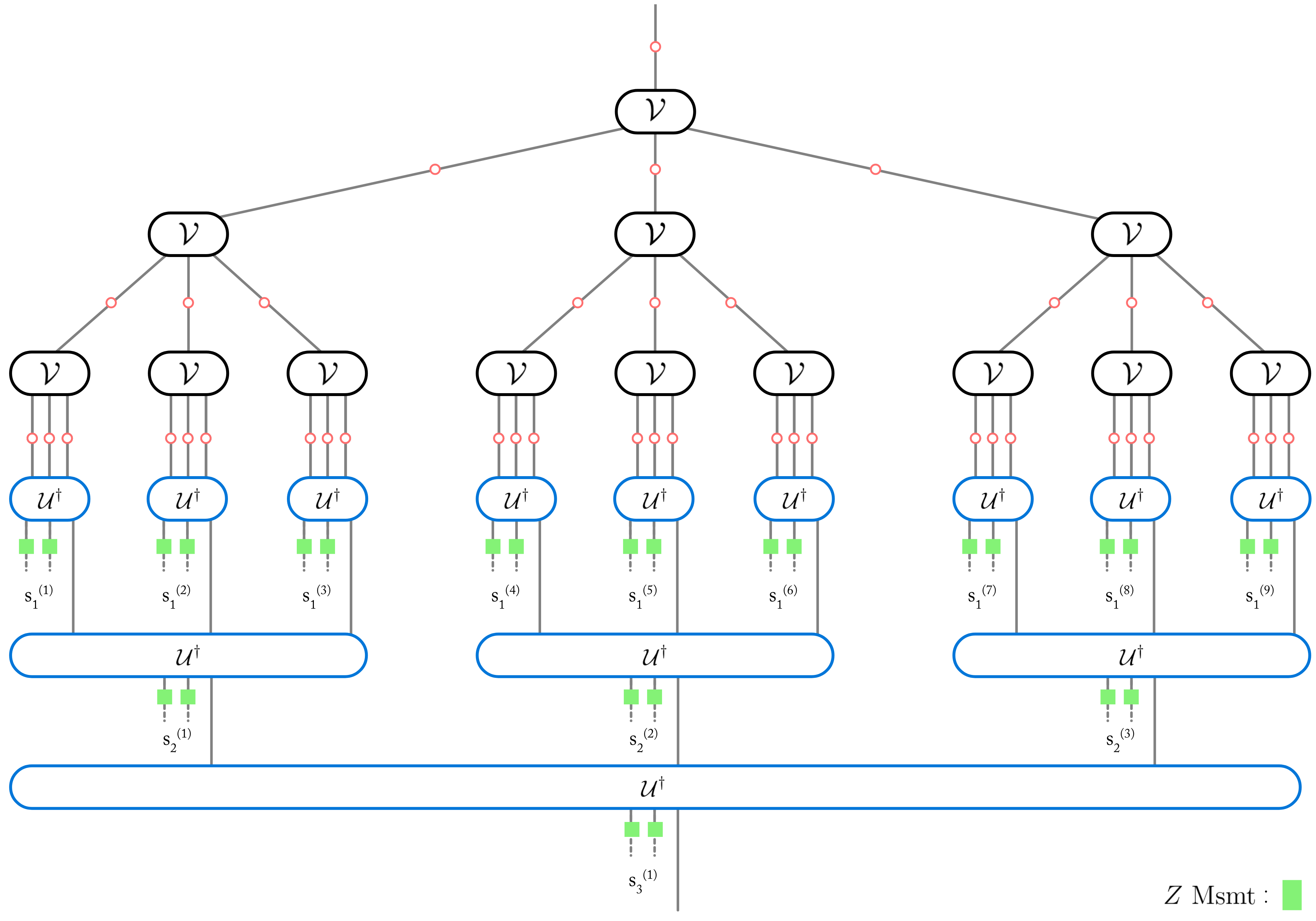
Figure 25: Fig. illustrates the optimal recovery circuit . While the upper-half of the figure is a tree with stabilizer encoder $\mathcal{V}$ along with Pauli noise $\mathcal{N}$ on each edge, the lower half is the application of the inverse unitary $\mathcal{U}_{T}^{\dagger}=U_{T}^{\dagger}(.)U_{T}$ on the output of the tree process. Note that $\mathcal{U}$ is the Clifford unitary corresponding to the stabilizer isometry $\mathcal{V}$. Upon inversion, we measure each of the ancillary qubits in the $Z$-basis to obtain the syndrome string. Here we see syndromes of the form $s^{(i)}_{n}$ indicated. Observe that the syndrome-acquisition circuit is a ‘reflection’ of the original tree circuit.

G.2 Recovery Algorithm

Consider a noisy stabilizer tree, defined in Sec. II, of the form,

$$\mathcal{E}_{T}(\rho)=\mathcal{N}^{\otimes b^{T}}\circ\prod_{j=0}^{T-1}\mathcal{V}^{\otimes b^{j}}\circ\mathcal{N}^{\otimes b^{j}}(\rho).$$ (264)

where $\mathcal{V}$ is a $1\rightarrow b$ qubit stabilizer isometry, and $\mathcal{N}$ is a single qubit Pauli noise. Let $U$ be the Clifford encoder as defined in Eq.(262). Note that 264 has a noise before the first encoding, and also after the tree on the leaves.

Considering Clifford encoders and Pauli channels ensures that the effective noise caused by the entire tree remains as Pauli noise. That is, the tree process can be understood as a noiseless $1\rightarrow b^{T}$ qubit stabilizer isometry, followed by a $b^{T}$ qubit Pauli noise. The essential task of recovery after a noisy tree process can, thus, be understood as computing the logical error component of the said Pauli noise process. To this end, we shall infer logical error by conditioning on syndrome data. Thus, the general recovery strategy can be summarized as,

1. Initially, input the state $\rho$ at the root; the output state of the noisy $1\rightarrow b^{T}$ qubit stabilizer tree process is $\mathcal{E}_{T}(\rho)$.

2. To this output state, apply the inverse of the encoder for the entire tree,

   $$U_{T}^{\dagger}=\prod_{j=0}^{T-1}{U^{\dagger}}^{\otimes b^{T-1-j}}.$$ (265)

3. Measure the $b^{T}-1$ auxilliary qubits in the $Z$-basis to record the syndrome string $\mathbf{s}_{T}$.

4. Construct and check the dictionary between syndrome strings and single-qubit logical error distributions, i.e., $p(L_{T}|\mathbf{s}_{T})$.

5. Apply ${\rm argmax}_{E}\ p(L_{T}|\mathbf{s}_{T})$ to the 0^th qubit to correct the most probable logical error.

Fig. 25 clarifies this inversion and syndrome-acquisition procedure. Observe that this decoding circuit is essentially a ‘reflection’ of the encoding tree. So we see that for a tree of depth $T$, we have a syndrome of length $b^{T}-1$, and thus, need to construct and search a dictionary over $2^{b^{T}-1}$ syndrome strings, which is clearly untenable. But thanks to the tree structure, there is a belief propagation algorithm that uses the syndrome data and computes this logical error distribution in $\mathcal{O}(b^{T-1})$ steps – an exponential improvement!

G.3 Ordering of syndrome strings

The tree structure provides a natural partitioning of the syndrome string. Consider a $b$-ary tree with $T$ levels. The entire syndrome is a bit string of length $b^{T}-1$. Denote this by $\mathbf{s}_{T}$. Observe that the entire tree can be characterized as the network that descends from the root edge. Similarly, let us consider the $b$ subtrees whose root edges are the $b$ children of the first encoder of the tree. Denote the syndrome string obtained from the $i^{\rm th}$ of these subtrees as $\mathbf{s}_{T-1}^{(i)}$, where the subscript $T-1$ indicates that the subtree is rooted in level-$T-1$. Each $\mathbf{s}_{T-1}^{(i)}$ will have length $b^{T-1}-1$. Finally define $s_{T}$ such that $s_{T}\cup(\cup_{i=1}^{b}\mathbf{s}_{T-1}^{(i)})=\mathbf{s}_{T}$. Observe that $s_{T}$ is the syndrome string of length $b-1$ obtained from measuring the $b-1$ ancillary qubits that are outputs of the inverse encoder during decoding, that corresponds ‘by reflection’ to the first encoder immediately below the root edge.

We can similarly define the syndrome string $\mathbf{s}_{t}^{(j)}$ for the $j^{\rm th}$ subtree whose root edge is in level-$t$. Observe that this indexing also provides a labeling for the subtrees via its root edge position $(j,t)$. We can, thus, say two edges $(j,t)$ and $(i,t-1)$ are adjacent when $(j,t)$ is the parent edge of $(i,t-1)$, denoted by $(j,t)\sim(i,t-1)$. Thus, holds the relation,

$$s^{(j)}_{t}\cup(\cup_{i:(j,t)\sim(i,t-1)}\mathbf{s}_{t-1}^{(i)})=\mathbf{s}^{(j)}_{t}.$$

The locality structure of trees ensures that the logical error $L^{(j)}_{t}$, associated to the $j^{\rm th}$ subtree rooted in level $t$, only depends on $\mathbf{s}_{t}^{(j)}$, and is independent of the rest of the syndrome string, i.e.

$$p(L^{(j)}_{t}|\mathbf{s}_{t})=p(L^{(j)}_{t}|\mathbf{s}_{t}^{(j)})\ .$$ (266)

In the following, we focus on calculating this conditional probability.

G.4 Belief Update Rule

Consider the root edge of the entire tree channel $\mathcal{E}_{T}$, i.e., level-T. Let us call the logical error for the entire tree $L_{T}$. This root qubit is firstly effected by a local Pauli noise $\mathcal{N}$, and then it is encoded in $b$ qubits via $\mathcal{V}$. Now consider the $b$ subtrees rooted at these $b$ children edges of $\mathcal{V}$. Label the logical error associated to each of these subtrees as error string $L_{T-1}=(L_{T-1}^{(1)},L_{T-1}^{(2)},...,L_{T-1}^{(b)})$ respectively. Let $\mathbf{s}_{T}$ label the syndrome string obtained from decoding the entire tree. Similarly, let $\mathbf{s}_{T-1}=(\mathbf{s}_{T-1}^{(1)},\mathbf{s}_{T-1}^{(2)},...\mathbf{s}_{T-1}^{(b)})$ indicate the syndrome set obtained from decoding the $b$ ‘level-${T-1}$’ subtrees noted just earlier. We shall also consider an intermediate tree that is rooted at the edge after the noise process $\mathcal{N}$, and whose logical error we denote by $L_{T}^{\prime}$. Observe that the entire tree and this intermediate tree are conditioned by the same syndrome $\mathbf{s}_{T}$ and differ only by the effect of single-qubit $\mathcal{N}$.

Thus, the crux of the BP algorithm is an update rule from,

$$p(L_{T-1}|\mathbf{s}_{T-1})\rightarrow p(L_{T}^{\prime}|\mathbf{s}_{T})\rightarrow p(L_{T}|\mathbf{s}_{T}).$$

The second update is simple as it is caused only by the single-qubit noise process $\mathcal{N}$. Given Pauli noise channel

$$\mathcal{N}(.)=r_{I}(.)+r_{x}X(.)X+r_{y}Y(.)Y+r_{z}Z(.)Z$$

on the edge prior to encoder, we define the transition probability between $E_{1}$ and $E_{2}$ in the Pauli group as

$$N(E_{1}|E_{2})=r_{E_{1}E_{2}}$$ (267)

where $E_{1}E_{2}$ is the matrix product of Pauli operators $E_{1}$ and $E_{2}$ upto global phase. Then,

$$p(L_{T}|\mathbf{s}_{T})=\sum_{L_{T}^{\prime}}{N}(L_{T}|L_{T}^{\prime})\ p(L_{T}^{\prime}|\mathbf{s}_{T})\ .$$ (268)

The first update is derived in the spirit of Eq.4 in Poulin (2006):

$$p(L_{T}^{\prime}|\mathbf{s}_{T}) =\sum_{L_{T-1}}\ p(L_{T}^{\prime}|L_{T},\mathbf{s}_{T})\ p(L_{T-1}|\mathbf{s}_{T})\ .$$ (269)

The logical error $L_{T}^{\prime}$ is completely determined by $L_{T-1}$ by considering its logical part, i.e., $\mathcal{L}(L_{T-1})$. Thus, $p(L_{T}^{\prime}|L_{T-1},\mathbf{s}_{T})=\delta[L_{T}^{\prime}=\mathcal{L}(L_{T-1})]$. Next we look at the second term. Recall that $\mathbf{s}_{T}=s_{T}\cup\mathbf{s}_{T-1}=s_{T}\cup(\cup_{i=1}^{b}\mathbf{s}_{T-1}^{(i)})$. Thus,

$$p(L_{T-1}|\mathbf{s}_{T}) =p(L_{T-1}|s_{T},\mathbf{s}_{T-1})=\frac{p(L_{T-1},s_{T},\mathbf{s}_{T-1})}{p(s_{T},\mathbf{s}_{T})}=\frac{p(s|L_{T-1},\mathbf{s}_{T-1})}{p(s_{T}|\mathbf{s}_{T-1})}\ p(L_{T-1}|\mathbf{s}_{T-1}).$$ (270)

The syndrome $s_{T}$ is completely determined by the $b$-qubit error string $L_{T-1}$. Thus, $p(s_{T}|L_{T-1},\mathbf{s}_{T-1})=\delta[s_{T}={\rm Synd}(L_{T-1})]$. By substituting these into 269,

$$p(L_{T}^{\prime}|\mathbf{s}_{T})=\sum_{L_{T-1}}\delta[L_{T}^{\prime}=\mathcal{L}(L_{T-1})]\ \delta[s_{T}={\rm Synd}(L_{T-1})]\frac{1}{p(s_{T}|\mathbf{s}_{T-1})}p(L_{T-1}|\mathbf{s}_{T-1})$$ (271)

where $\mathcal{L}(E)$ is the logical error associated to $E$ and ${\rm Synd}(E)$ is the syndrome bitstring associated to $E$ (Refer to subsection G.1). An important final observation is that the logical errors associated to different non-overlapping subtrees are independent. This is because the noise processes within the tree are local to each edge. The $b$ subtrees, whose logical errors constitute one term of $L_{T-1}$ each, are also non-overlapping. Thus, logical errors $\{L_{T-1}^{(i)}\}_{i}$ are independent from each other, where $i$ indexes the subtree. Recall that $\mathbf{s}_{T-1}=\{\mathbf{s}_{T-1}^{(i)}\}_{i}$. Thus, the first update is,

$$p(E^{\prime}_{T}|\mathbf{s}_{T})=\sum_{L_{T-1}}\delta[L_{T}^{\prime}=\mathcal{L}(L_{T-1})]\ \delta[s_{T}={\rm Synd}(L_{T-1})]\times\frac{1}{p(s_{T}|\mathbf{s}_{T-1})}\prod_{i}p(L^{(i)}_{T-1}|\mathbf{s}^{(i)}_{T-1})$$ (272)

Combining the first and second updates gives us,

$$p(L_{T}|\mathbf{s}_{T})=\sum_{L_{T}^{\prime}}{N}(L_{T}|L_{T}^{\prime})\sum_{L_{T-1}}\delta[L_{T}^{\prime}=\mathcal{L}(L_{T-1})]\delta[s_{T}={\rm Synd}(L_{T-1})]\times\frac{1}{p(s_{T}|\mathbf{s}_{T-1})}\prod_{i}p(L^{(i)}_{T-1}|\mathbf{s}^{(i)}_{T-1})$$ (273)

If we change the order of summation and define,

$$f_{s_{T}}(L_{T},L_{T-1}):=\sum_{L_{T}^{\prime}}\delta[L_{T}^{\prime}=\mathcal{L}(L_{T-1})]\delta[s_{T}={\rm Synd}(L_{T-1})]\ {N}(L_{T}|L_{T}^{\prime})=\ \delta[s_{T}={\rm Synd}(L_{T-1})]\ \mathcal{N}(L_{T}|\mathcal{L}(L_{T-1}))$$ (274)

we get,

$$p(L_{T}|\mathbf{s}_{T})=\sum_{L_{T-1}}f_{s_{T}}(L_{T},L_{T-1})\frac{1}{p(s_{T}|\mathbf{s}_{T-1})}\prod_{i}p(L^{(i)}_{T-1}|\mathbf{s}^{(i)}_{T-1}),$$ (275)

where $\mathbf{s}_{T}=(s_{T},\mathbf{s}_{T-1})$. If we consider trees with no noise within them, ${N}(L_{T}|L_{T}^{\prime})=\delta(L_{T}=L_{T}^{\prime})$. Thus, $f_{s_{T}}(L_{T},L_{T-1})=\delta[L_{T}=\mathcal{L}(L_{T-1})]\ \delta[s_{T}={\rm Synd}(L_{T-1})]$, which is equivalent to Eq.4 in Poulin (2006). Finally using the independence of non-overlapping subtrees, we can repeat this procedure for $p(L^{(i)}_{T-1}|\mathbf{s}^{(i)}_{T-1})$ for each $i$, and further on propagate until the leaves of the tree. That is to say, $p(L^{(j)}_{0})={N}(L^{(j)}_{0}|I)$ is set as the terminal condition of recursion for all $j$.

G.5 Optimality & Efficiency

Firstly note that $p(L_{T}|\mathbf{s}_{T})$ contains all the relevant information to make a decision regarding the logical error that occurred within the entire tree as seen in Sec. G.2. And its computation is, as noted, via a BP algorithm on a tree-like factor graph. From theorem 14.1 in Mezard and Montanari (2009), we note that BP on tree-like factor graphs is exact. Thus, optimality is ensured by our BP algorithm. Another way to observe optimality is notice that the application of the inverse encoder, followed by the syndrome measurement is a completely reversible process: we can re-apply the entire $1\rightarrow b^{T}$ qubit encoder to the single qubit that is the output of the decoding procedure; and then based on the syndrome, we can apply the associated error as defined in Sec. G.1; this would give us the output state of the tree. Thus, we have not discarded any information when computing $p(L_{T}|\mathbf{s}_{T})$.

The efficiency of this algorithm is a consequence of the local tree structure that allows local propagation of belief. In principle, for a $b$-ary tree of $T$ levels, we have $b^{T}$ leaves. And thus, we must perform summations of probability distribution over $\mathcal{O}(2^{(b^{T-1})})$ bitstrings. Such a double-exponential computation is untenable. The aforementioned BP algorithm instead considers operations restricted to each vertex. This entails summations over $\mathcal{O}(2^{b})$ at each vertex. We consider this for all $\mathcal{O}(b^{T-1})$ vertices, which is a summation over $\mathcal{O}(2^{b}\times b^{T-1})$ terms for the entire tree. Thus, we have here an exponential summation that is a drastic improvement in our efficiency.

G.6 Restricting to Single-direction

Consider the special case where our stabilizer code is a CSS code with a standard encoder. Along with this, let the Pauli noise be independent $X$ and $Z$ noise. We saw in Sec. VIII that these can be studied as dephased trees, where we study the evolution of bitstrings over $\{0,1\}$, rather than $\{I,X,Y,Z\}$. We can perform optimal recovery using BP on these dephased trees too. This is equivalent to looking at recovery only in either the $Z$ or $X$-direction.

To this end, the aforementioned BP algorithm is only slightly modified: Let us focus on the $Z$-direction. In this case, $X,Y$ errors are considered bit-flip errors (associated to error bit value $1$), but not $I,Z$ errors (associated to error bit value $0$). Thus, the errors $L^{(j)}_{n}$ in the single-direction BP procedure will be bitstrings.

The single-direction analog of BP update rule in Eq.(275) requires us to revisit the functions ${\rm Synd(E)}$ and $\mathcal{L}(E)$ for an error $E$. Firstly, syndromes are obtained by measuring the generators of stabilizers. If we are only interested in the $Z$-direction, we must only consider the $Z$-type stabilizer generators of the CSS code. This can formulated via a Check-Matrix. The check-matrix for a $Z$-dephased CSS encoder is the bit-string form of the $Z$-stabilizer generators, where the bit-string form of each generator forms one row of the check-matrix. The co-domain for the check-matrix we call the syndrome space. For e.g., in the Shor-9 code, the $Z$-stabilizer generators are $Z_{1}Z_{2}$, $Z_{2}Z_{3}$, $Z_{4}Z_{5}$, $Z_{5}Z_{6}$, $Z_{7}Z_{8}$ and $Z_{8}Z_{9}$, where the subscripts label the $9$ output qubits of the code. Thus, the check-matrix becomes,

$$M=\begin{pmatrix}1&1&0&0&0&0&0&0&0\\ 0&1&1&0&0&0&0&0&0\\ 0&0&0&1&1&0&0&0&0\\ 0&0&0&0&1&1&0&0&0\\ 0&0&0&0&0&0&1&1&0\\ 0&0&0&0&0&0&0&1&1\end{pmatrix}.$$ (276)

So in this instance, the syndrome associated to any 9 bit string $x$ will be the 6 bit string $s=Mx$. The logical component associated to $E$ can be constructed as follows: start with the function $\mathcal{L}(E)$. Let $X_{i}$ indicate the operator string with $X$ in the $i^{\rm th}$ position, and identity everywhere else, i.e., $X_{1}=XII..II$, and so on. Define

$$\mathbb{L}=({x_{1}}\ {x_{2}}\ ...\ {x_{b}}),$$

where ${x_{i}}$ is defined using the relation $\mathcal{L}(X_{i})=\pm{Z^{z_{i}}}\times{X^{x_{i}}}$ for all $i$ (this exponent notation is defined in Sec. III.5). Then we get the logical component of error string $E$ by the multiplication $\mathbb{L}E$. For instance, in the Shor-9 code,

$$\mathbb{L}=(0\ \ 1\ \ 0\ \ 0\ \ 1\ \ 0\ \ 0\ \ 1\ \ 0).$$

The syndrome-acquisition circuit is similar to Fig. 25, where at each decoding vertex we apply the check matrix to obtain the syndrome string, and then decode to the logical component. We order the syndromes just as done earlier by considering the subtrees from which these syndromes emerge.

To obtain the belief propagation rule for a single direction, we replace $\mathcal{L}(E)\rightarrow\mathbb{L}E$, and ${\rm Synd}(E)\rightarrow ME$ in 275. Thus, the belief propagation rule from level $t-1$ to $t$ is,

$$p(L_{t}|\mathbf{s}_{t})=\sum_{L_{t-1}}f_{s_{t}}(L_{t},L_{t-1})\frac{1}{p(s_{t}|\mathbf{s}_{t-1})}\prod_{i}p(L^{(i)}_{t-1}|\mathbf{s}^{(i)}_{t-1}),$$ (277)

where

$$f_{s_{t}}(L_{t},L_{t-1}):=\sum_{L_{t}^{\prime}}\delta[L_{t}^{\prime}=\mathbb{L}(L_{t-1})]\delta[s=ML_{t-1}]\ {N}(L_{t}|L_{t}^{\prime})=\ \delta[s=ML_{t-1}]\ {N}(L_{t}|\mathbb{L}(L_{t-1})).$$ (278)

Here each of the $L$’s are bitstrings associated to logical errors and ${N}$ is a local bit-flip ($X$-error) transition matrix $N(E_{1}|E_{2})=p+(1-2p)\times\delta(E_{1}=E_{2})$.

Note regarding noise at the root – The presentation above if for a tree with noise at the root. We can very easily modify this analysis for a tree without at the root. We use that in the very last step of decoding (i.e., $t=T$), we modify Eq.(278) as

$$f_{s_{T}}(L_{T},L_{T-1}):=\sum_{L_{T}^{\prime}}\delta[L_{T}^{\prime}=\mathbb{L}(L_{T-1})]\delta[s=ML_{T-1}]\ {N}(L_{T}|L_{T}^{\prime})=\ \delta[s=ML_{T-1}]\ \delta(L_{T}=\mathbb{L}(L_{T-1})).$$

G.7 Numerics: Classical $3$-ary tree

As a sanity check, we applied this optimal recovery algorithm to a classical tree with branching number 3, and bit-flip error on each edge. This case has been studied in Evans et al. (2000) and we know that the asymptotic phase transition is at $(1-3^{-\frac{1}{2}})/2=\sim 0.21$. The figure below plots the overall error after recovery as a function of bit-flip error rate within the tree.

The logical error saturates for 11 layers around $\sim 0.27$. With increasing depth, the transition progresses lower. For larger depths we should expect it to approach the optimal $\sim 0.21$. Additionally, for $T=1$ layer, we can compute the exact logical error rate, i.e., $3(1-p)p^{2}+p^{3}$. We see that our Monte Carlo simulation matches the exact computation.

G.8 Numerics: Optimal recovery of Shor-9 code tree

We use this belief-propagation algorithm to compute the optimal recovery probability for the Shor-9 code. Let us consider the $Z$-direction distinguishability first. As we noted in the text earlier, for such $Z$-dephased Shor-9 trees with the same encoder and noise at each vertex, we just need to specify $M$ and $\mathbb{L}$. As we saw,

$$M=\begin{pmatrix}1&1&0&0&0&0&0&0&0\\ 0&1&1&0&0&0&0&0&0\\ 0&0&0&1&1&0&0&0&0\\ 0&0&0&0&1&1&0&0&0\\ 0&0&0&0&0&0&1&1&0\\ 0&0&0&0&0&0&0&1&1\end{pmatrix},$$ (279)

and thus,

$$\mathbb{L}=(0\ 1\ 0\ 0\ 1\ 0\ 0\ 1\ 0).$$ (280)

We shall perform a Monte Carlo simulation of our algorithm.

Set-up – Consider a $b$-ary tree of $T$ levels with bit-flip noise of $p$ on each edge. For the Shor-9 case, we have $b=9$. Initially sample an error bitstring $L_{T}$ of length $b^{T}$ from the tree process. To $L_{T}$, we apply the ‘reflected’ recovery circuit shown in Fig. 25. The logical error bit is computed by applying

$$\mathbb{L}\circ...\circ\mathbb{L}^{\otimes b^{T-2}}\circ\mathbb{L}^{\otimes b^{T-1}}=:\mathbb{L}_{T}.$$

We shall denote the logical error bit by $\mathbb{L}_{T}L_{T}$. We also apply $M$ to every block at each step in the circuit to acquire all the syndromes. We know the local independent bit-flip probability on each of the edges, that is,

$${N}(0|0)={N}(1|1)=(1-p);\ {N}(1|0)={N}(0|1)=p.$$

Using these, we compute all the $f_{s}(.,.)$ values. And for the same reason, we shall start with the initial belief probability distribution,

$$p(L_{0})=\prod_{i\in{\rm leaves}}p(L^{(i)}_{1})$$

where each $p(L^{(i)}_{0})=\{0:1-p,1:p\}$. We shall apply our message-passing algorithm to all this syndrome data based on the factor tree detailed in Sec. G.4, and the aforementioned initial belief distribution. For any given sampled $L_{T}$, we check whether ${\rm argmax}p_{L_{T}}(L_{T}|\mathbf{s}_{T})=\mathbb{L}_{T}L_{T}$? The effective error after BP reconstruction is the number of times these values do not match. These are presented in Section VII.2

$X$-direction distinguishability– We can repeat the above computation by considering the $X$-direction distinguishability instead of $Z$. This entails a change in $M$ and $\mathbb{L}$. For the check-matrix, we must now consider the $X$-stabilizers as the rows of $M$, giving,

$$M=\begin{pmatrix}1&1&1&1&1&1&0&0&0\\ 0&0&0&1&1&1&1&1&1\end{pmatrix}.$$ (281)

and

$$\mathbb{L}=(0\ 0\ 0\ 1\ 1\ 1\ 0\ 0\ 0).$$ (282)

We use the same initial distribution as earlier and same factor tree for message-passing. Results for this are plotted in Sec. VII.2.

Note regarding Estimated Mean & Error – Observe that after randomly generating the effect of noise, the BP algorithm is a completely deterministic function, and thus whether is recovered correctly or not is also a deterministic function. So for a specific noise parameter setting, we have a Bernoulli random variable that outputs success or failure of the recovery procedure. We are to compute the parameter of this Bernoulli random, that is the probability of success/failure.

Our Monte Carlo simulation for a given noise setting outputs such a data set $\mathbf{x}$ of $N$ runs comprised of $1$ (success) or $0$ (failure). Maximum likelihood estimation on this data entails that success probability is the sample mean $\mathbb{E}({\mathbf{x}})=\sum_{x\in\mathbf{x}}x/N$, and the estimate’s variance is ${\rm Var}(\mathbf{x})=\mathbb{E}({\mathbf{x}})(1-\mathbb{E}({\mathbf{x}}))/N\leq 1/4N$. So to have a standard deviation of $\mathcal{O}(0.01)$, we need $\sim 2500$ samples.

G.9 Numerics: Steane-7 Code

When we use the standard Steane-7 encoder, defined by $Z$-type stabilizers, in a tree that is subject to independent $X$ and $Z$ single qubit errors, we get that,

$$M=\begin{pmatrix}1&0&0&0&1&1&1\\ 0&1&0&1&0&1&1\\ 0&0&1&1&1&0&1\\ \end{pmatrix}.$$ (283)

and

$$\mathbb{L}=(0\ 0\ 0\ 1\ 1\ 1\ 0).$$ (284)

The noises are single bit-flip errors. Using these we can compute the optimal recovery for trees (which is plotted in Sec. VII.2). An important property of the Steane-7 CSS code is that its self-dual. Thus, the behavior of $Z$-direction is exactly the same as $X$. Thus, we obtain the same recovery performance, and thus, same noise threshold.

Appendix H Dephased Encoders

In Sec. VIII we explained the idea of dephasing trees obtained from the standard (or, anti-standard) encoders of CSS codes to obtain an equivalent problem about the propagation of information on classical trees, which is a variant of the standard broadcasting problem studied in, e.g., Evans et al. (2000). This equivalency is based on the fact that for CSS codes $X$ and $Z$ errors can be corrected independently, and therefore adding one type of error to the tree does not affect the probability of logical of error for the other type.

For completeness, here we state and prove this property in a more formal language.

Proposition 11.

Let $Z_{L}\in\langle iI,Z\rangle^{\otimes n}$ be a logical operator of a CSS code and $|0\rangle_{L}$ and $|1\rangle_{L}$ be two orthogonal eigenstates of $Z_{L}$ in the code subspace, satisfying $|c\rangle_{L}=(-1)^{c}Z_{L}|c\rangle_{L}:\ c=0,1$. Suppose the qubits are subjected to noise channel $\mathcal{E}_{z}\circ\mathcal{E}_{x}=\mathcal{E}_{x}\circ\mathcal{E}_{z}$, where $\mathcal{E}_{x}$ only involves Pauli $X$ errors and $\mathcal{E}_{z}$ only involves Pauli $Z$ errors (This means $Z$ and $X$ error are independent, whereas $X$ (or, $Z$) errors on different qubits can be correlated). Then, there exists a quantum channel $\mathcal{R}$, such that

$$\mathcal{R}\circ\mathcal{E}_{z}\circ\mathcal{E}_{x}(|c\rangle\langle c|_{L})=\mathcal{E}_{x}(|c\rangle\langle c|_{L})\ \ \ :c=0,1\ .$$ (285)

Furthermore, given state $\mathcal{E}_{z}\circ\mathcal{E}_{x}(|c\rangle\langle c|_{L})$ with unknown $c=0,1$, the optimal strategy for determining the value of bit $c$ is measuring all the qubits in the $Z$ basis, followed by a classical processing of the outcomes.

Proof.

We prove the first part of the proposition by constructing the said recovery map $\mathcal{R}$. Without loss of generality we can restrict our attention to the case of 2-dimensional codes. If the code subspace has dimension more than 2, we focus on the 2-dimensional subspace spanned by $|0\rangle_{L}$ and $|1\rangle_{L}$, which will also be a CSS code.

In particular, there exists a logical operator $X_{L}\in\langle iI,X\rangle^{\otimes n}$, and

$$S^{z}_{j} \in\langle iI,Z\rangle^{\otimes n}:j=2,\cdots,n_{z}+1$$ (286)

$$S^{x}_{k} \in\langle iI,X\rangle^{\otimes n}:k=n_{z}+2,\cdots,n$$ (287)

where $\{S^{z}_{j}\}$ and $\{S^{x}_{k}\}$ are $n_{z}$ and $n_{x}$ independent $Z$ and $X$ stabilizers and $n=n_{x}+n_{z}+1$. Using the standard results in the theory of stabilizer codes we know that any such code has an encoder such that

$$|c\rangle_{L}=W(|c\rangle\otimes|0\rangle^{\otimes n_{z}}\otimes|0\rangle^{\otimes n_{x}})\ \ \ \ \ \ \ \ :\ c=0,1\ ,$$ (288)

and

$$WZ_{1}W^{\dagger} =Z_{L}\ \ ,\ WX_{1}W^{\dagger}=X_{L}$$ (289)

$$WZ_{j}W^{\dagger} =S^{z}_{j}\ \ \ \ \ \ :\ j=2,\cdots n_{z}+1$$ (290)

$$WZ_{k}W^{\dagger} =S^{x}_{k}\ \ \ \ \ \ :\ k=n_{z}+2,\cdots,n_{x}+n_{z}+1\ .$$ (291)

In other words, under unitary $W^{\dagger}$ the Hilbert space of $n$ physical qubits decomposes as

$$(\mathbb{C}^{2})^{\otimes n}=\mathbb{C}^{2}\otimes\mathcal{H}_{\text{z-stab}}\otimes\mathcal{H}_{\text{x-stab}}$$ (292)

where $\mathcal{H}_{\text{z-stab}}=(\mathbb{C}^{2})^{\otimes n_{z}}$ and $\mathcal{H}_{\text{x-stab}}=(\mathbb{C}^{2})^{\otimes n_{x}}$. The fact that the code is a CSS code implies that for any $X$ error $\textbf{X}^{\textbf{x}}$ with $\textbf{x}\in\{0,1\}^{n}$ and $Z$ error $\textbf{Z}^{\textbf{z}}$ with $\textbf{z}\in\{0,1\}^{n}$ it holds that

$$W^{\dagger}\textbf{X}^{\textbf{x}}\textbf{Z}^{\textbf{z}}|c\rangle_{L} =\pm\big{(}X^{x_{L}(\textbf{x})}Z^{z_{L}(\textbf{z})}|c\rangle\big{)}\otimes|\mathbf{s}_{z}(\textbf{x})\rangle\otimes|\mathbf{s}_{x}(\textbf{z})\rangle\ .$$ (293)

where $\mathbf{s}_{z}(\mathbf{x})$ is the syndrome string associated to $Z$ stabilizer measurements of $X$ error $\textbf{X}^{\textbf{x}}$ (and vice versa for $\mathbf{s}_{x}(\mathbf{z})$). Thus,

$$W^{\dagger}(\mathcal{E}_{x}\circ\mathcal{E}_{z}(\ket{c}\bra{c}_{L}))W=\sum_{\mathbf{x},\mathbf{z}}p(\mathbf{x},\mathbf{z})({X}^{x_{L}(\textbf{x})}{Z}^{z_{L}(\textbf{z})}|c\rangle\langle c|_{L}{Z}^{z_{L}(\textbf{z})}{X}^{x_{L}(\textbf{x})})\otimes\ket{\mathbf{s}_{z}(\mathbf{x})}\bra{\mathbf{s}_{z}(\mathbf{x})}\otimes\ket{\mathbf{s}_{x}(\mathbf{z})}\bra{\mathbf{s}_{x}(\mathbf{z})}$$ (294)

Recall $\ket{c}_{L}$ is a logical $Z$ state, i.e., ${Z}_{L}|c\rangle=\pm|c\rangle$. Noting the independence of $X$ and $Z$ errors, we have $p(\mathbf{x},\mathbf{z})=p(\mathbf{x})p(\mathbf{z})$. Thus,

$$W^{\dagger}(\mathcal{N}_{x}\circ\mathcal{N}_{z}(\ket{c}\bra{c}_{L}))W=\sum_{\mathbf{x}}p(\mathbf{x})({X}^{x_{L}(\textbf{x})}|c\rangle\langle c|_{L}{X}^{x_{L}(\textbf{x})})\otimes\ket{\mathbf{s}_{z}(\mathbf{x})}\bra{\mathbf{s}_{z}(\mathbf{x})}\otimes\sum_{\mathbf{z}}p(\mathbf{z})\ket{\mathbf{s}_{x}(\mathbf{z})}\bra{\mathbf{s}_{x}(\mathbf{z})}$$ (295)

We see here that $\mathbb{C}^{2}\otimes\mathcal{H}_{\rm z-stab}$ is uncorrelated with $\mathcal{H}_{\rm x-stab}$. Furthermore, all the information regarding $Z$ errors is within $\mathcal{H}_{\rm x-stab}$. So replacing this subsystem with $\ket{0}^{\otimes n_{z}}$ allows us to discard the effect of $\mathcal{N}_{z}$. Thus, in summary, the recovery channel we want is,

$$\mathcal{R}(\cdot)=W\Big{(}\textrm{Tr}_{\text{x-stab}}(W^{\dagger}(\cdot)W)\otimes|0\rangle\langle 0|^{\otimes n_{z}}\Big{)}W^{\dagger}.$$ (296)

To show the second part of the proposition, suppose one measures all qubits in $\{|0\rangle,|1\rangle\}$ basis. If we ignore the outcomes of all measurements, i.e., if we dephase all qubits in the $Z$ basis, we obtain state $\mathcal{D}_{z}^{\otimes n}\circ\mathcal{E}_{z}\circ\mathcal{E}_{x}(|c\rangle\langle c|_{L})$. Since $\mathcal{D}_{z}^{\otimes n}\circ\mathcal{E}_{z}$ only contains $Z$ errors, using the first part of the proposition, we know that there exists a recovery process that transforms state $\mathcal{D}_{z}^{\otimes n}\circ\mathcal{E}_{z}\circ\mathcal{E}_{x}(|c\rangle\langle c|_{L})$ to $\mathcal{E}_{z}\circ\mathcal{E}_{x}(|c\rangle\langle c|_{L})$. This means that, regardless of the figure of merit, the optimal strategy for discriminating states $\mathcal{E}_{z}\circ\mathcal{E}_{x}(|0\rangle\langle 0|_{L})$ and $\mathcal{E}_{z}\circ\mathcal{E}_{x}(|1\rangle\langle 1|_{L})$ can start with a measurement of all qubits in the $Z$ basis, followed by a classical processing of the outcomes of $Z$ measurements (which is the only information remaining in a fully dephased state). ∎

H.1 Example: Generalized Shor Code

The dephased tree of generalized Shor codes $[[n^{2},1,n]]$ is where we have classical encoders that are alternatingly concatenated. We label them $\mathbb{M}_{1}$ and $\mathbb{M}_{2}$, and are defined:

$$\mathbb{M}_{1}: \ P_{z}(0^{\otimes n}|0)=1$$

$$\ P_{z}(1^{\otimes n}|1)=1$$ (297)

$$\mathbb{M}_{2}: \ P_{z}(\mathbf{w}|0)=\frac{1}{2^{n-1}},\ {\rm when}\ |\mathbf{w}|=0\ {\rm mod\ 2}$$

$$\ P_{z}(\mathbf{w}|1)=\frac{1}{2^{n-1}},\ {\rm when}\ |\mathbf{w}|=1\ {\rm mod\ 2}$$ (298)

where $|\mathbf{w}|$ is the Hamming weight of $\mathbf{w}$. For instance, the usual Shor-9 code corresponds to $n=3$, and the specific maps are,

$$\mathbb{M}_{1}: \ P_{z}(000|0)=1$$

$$\ P_{z}(111|1)=1$$ (299)

$$\mathbb{M}_{2}: \ P_{z}(\mathbf{w}|0)=1/4,\ {\rm when}\ \mathbf{w}\in\{000,011,101,110\}$$

$$\ P_{z}(\mathbf{w}|1)=1/4,\ {\rm when}\ \mathbf{w}\in\{111,100,010,001\}$$ (300)

Thus, the encoder becomes $\mathbb{M}_{1}^{\otimes n}\circ\mathbb{M}_{2}$, from $1\rightarrow n^{2}$ bits. After every encoded layer, we have local independent bit-flip error on all these bits, which corresponds to $X$ (or $Z$) error channel between concatenated Shor encoder layers.

Considering these encoders in the opposite order, i.e., $\mathbb{M}_{2}^{\otimes n}\circ\mathbb{M}_{1}$ corresponds to dephasing in the conjugate basis, i.e., $X$ to $Z$ and vice versa.

H.2 Summary of Open Classical Problems

Study of novel dephased trees can be summarized into three succinctly stated classical tree problems, that still remain open problems. We list them in order of reducing generality. From here on, $\overline{1}$ is a bitsring with all $1$’s and ‘$+$’ is bit-wise addition modulo 2.

Problem I – Consider a tree-like circuit. Each vertex is associated to an encoder that maps one bit, $b$, to $n$ bitstring, $x$, probabilistically. This encoder is, thus, characterized by the conditional probability distribution $p(x|b)$ such that $p(x|b)=p(x+\overline{1}|b+1)$. This setup is general in that it also subsumes cases with binary symmetric channels (e.g., bit-flip noise channels) before or after the encoder.

Problem II – Here we focus on an important special case of Problem I, where $p(x|b)$ can be realized by adding local uncorrelated bit-flip noise on the output bits which are sampled from a distribution $q(x|b)$. Here, $q(x|b)$ has the property that $q(x|b=0)$ and $q(x|b=1)$ have disjoint support. So graphically, the vertices of the tree are associated to the aforementioned $q(x|b)$ encoder, and the edges are associated with bit-flip channels of error $\epsilon$.

More specifically, we are interested in the case where $q(x|b=0)$ is a uniform distribution over a subspace of bit strings, and $q(x|b=1)=q(x+\overline{1}|b=0)$, i.e, its complement. This restriction is interesting because the encoder by itself is not noisy (due to the disjoint support), although it might make the encoded information more sensitive to noise. Dephased trees of Steane codes and Generalized Shor Codes satisfy said property.

Problem III – We focus on the classical version of generalized Shor codes $[[n^{2},1,n]]$. Here we have two encoders from $1\rightarrow n$ bits that are alternatingly concatenated. We label them $\mathbb{M}_{1}$ and $\mathbb{M}_{2}$, and are defined:

$$\mathbb{M}_{1}:\ 0\mapsto 0^{\otimes n}$$

$$1\mapsto 1^{\otimes n}$$ (301)

$$\mathbb{M}_{2}:\ 0\mapsto{\rm uniformly\ random\ over\ even\ Hamming\ wt.}$$

$$1\mapsto{\rm uniformly\ random\ over\ odd\ Hamming\ wt.}$$ (302)

The encoder associated to each vertex is $\mathbb{M}_{1}^{\otimes n}\circ\mathbb{M}_{2}$, from $1\rightarrow n^{2}$ bits. For instance, the usual Shor-9 code corresponds to $n=3$, and the specific maps are,

$$\mathbb{M}_{1}:\ 0\mapsto 000$$

$$1\mapsto 111$$ (303)

$$\mathbb{M}_{2}:\ 0\mapsto{\rm Unif}\{000,011,101,110\}$$

$$1\mapsto{\rm Unif}\{111,100,010,001\}$$ (304)

Note that bit-flip noise here occurs after $\mathbb{M}_{1}^{\otimes n}\circ\mathbb{M}_{2}$, not in between them. The case where we switch the order of the encoders, i.e., $\mathbb{M}_{2}^{\otimes n}\circ\mathbb{M}_{1}$, corresponds to measuring in the conjugate basis, and is also of interest. $\mathbb{M}_{2}$ is, in some sense, maximally sensitive to noise. That is, an error on any of the $n$ children of $\mathbb{M}_{2}$ is equivalent to an error on the input bit. This is an extreme illustration of the comment made in Problem II.

A thorough analysis of these classical tree problems remains an open research direction in classical network theory. We presented partial progress regarding these questions in Appendix sections D.3 and G.6.

References

- Preskill (2018) J. Preskill, Quantum 2, 79 (2018), ISSN 2521-327X, URL https://doi.org/10.22331/q-2018-08-06-79.
- Gullans and Huse (2020a) M. J. Gullans and D. A. Huse, Phys. Rev. X 10, 041020 (2020a), URL https://link.aps.org/doi/10.1103/PhysRevX.10.041020.
- Gullans and Huse (2020b) M. J. Gullans and D. A. Huse, Phys. Rev. Lett. 125, 070606 (2020b), URL https://link.aps.org/doi/10.1103/PhysRevLett.125.070606.
- Skinner et al. (2019) B. Skinner, J. Ruhman, and A. Nahum, Phys. Rev. X 9, 031009 (2019), URL https://link.aps.org/doi/10.1103/PhysRevX.9.031009.
- Li et al. (2019) Y. Li, X. Chen, and M. P. A. Fisher, Phys. Rev. B 100, 134306 (2019), URL https://link.aps.org/doi/10.1103/PhysRevB.100.134306.
- Von Neumann (1956) J. Von Neumann, Automata studies 34, 43 (1956).
- Pippenger (1985) N. Pippenger, in 26th Annual Symposium on Foundations of Computer Science (sfcs 1985) (IEEE, 1985), pp. 30–38.
- Pippenger (1988) N. Pippenger, IEEE Transactions on Information Theory 34, 194 (1988).
- Benjamini et al. (1998) I. Benjamini, R. Pemantle, and Y. Peres, The Annals of Probability 26, 1198 (1998), URL https://doi.org/10.1214/aop/1022855749.
- Kesten and Stigum (1966) H. Kesten and B. P. Stigum, The Annals of Mathematical Statistics 37, 1211 (1966), ISSN 00034851, URL http://www.jstor.org/stable/2239076.
- Evans et al. (2000) W. Evans, C. Kenyon, Y. Peres, and L. J. Schulman, Ann. Appl. Probab. 10, 410 (2000), URL https://doi.org/10.1214/aoap/1019487349.
- Lyons and Peres (2016) R. Lyons and Y. Peres, Probability on Trees and Networks, vol. 42 of Cambridge Series in Statistical and Probabilistic Mathematics (Cambridge University Press, New York, 2016), ISBN 978-1-107-16015-6, available at https://rdlyons.pages.iu.edu/, URL http://dx.doi.org/10.1017/9781316672815.
- Mossel (2001) E. Mossel, The Annals of Applied Probability 11, 285 (2001), ISSN 10505164, URL http://www.jstor.org/stable/2667270.
- Mossel and Peres (2003) E. Mossel and Y. Peres, The Annals of Applied Probability 13, 817 (2003), ISSN 10505164, URL http://www.jstor.org/stable/1193228.
- Wootters and Zurek (1982) W. K. Wootters and W. H. Zurek, Nature 299, 802 (1982).
- Barnum et al. (1996) H. Barnum, C. M. Caves, C. A. Fuchs, R. Jozsa, and B. Schumacher, Phys. Rev. Lett. 76, 2818 (1996), URL https://link.aps.org/doi/10.1103/PhysRevLett.76.2818.
- Rahn et al. (2002) B. Rahn, A. C. Doherty, and H. Mabuchi, Phys. Rev. A 66, 032304 (2002), URL https://link.aps.org/doi/10.1103/PhysRevA.66.032304.
- Poulin (2006) D. Poulin, Physical Review A 74, 052333 (2006).
- Shi et al. (2006) Y.-Y. Shi, L.-M. Duan, and G. Vidal, Phys. Rev. A 74, 022320 (2006), URL https://link.aps.org/doi/10.1103/PhysRevA.74.022320.
- Roberts and Stanford (2013) D. A. Roberts and D. Stanford, Journal of High Energy Physics 2013, 1 (2013).
- Almheiri et al. (2015) A. Almheiri, X. Dong, and D. Harlow, Journal of High Energy Physics 2015, 1 (2015).
- Pastawski et al. (2015) F. Pastawski, B. Yoshida, D. Harlow, and J. Preskill, Journal of High Energy Physics 2015, 1 (2015).
- Shor (1995) P. W. Shor, Phys. Rev. A 52, R2493 (1995), URL https://link.aps.org/doi/10.1103/PhysRevA.52.R2493.
- Aharonov and Ben-Or (2008) D. Aharonov and M. Ben-Or, SIAM Journal on Computing (2008).
- Knill et al. (1996) E. Knill, R. Laflamme, and W. Zurek, arXiv preprint quant-ph/9610011 (1996).
- Gottesman (2014) D. Gottesman, Fault-tolerant quantum computation with constant overhead (2014), eprint 1310.2984.
- Chamberland et al. (2016) C. Chamberland, T. Jochym-O’Connor, and R. Laflamme, Phys. Rev. Lett. 117, 010501 (2016), URL https://link.aps.org/doi/10.1103/PhysRevLett.117.010501.
- Aharonov (2000) D. Aharonov, Phys. Rev. A 62, 062311 (2000), URL https://link.aps.org/doi/10.1103/PhysRevA.62.062311.
- Harrow and Nielsen (2003) A. W. Harrow and M. A. Nielsen, Phys. Rev. A 68, 012308 (2003), URL https://link.aps.org/doi/10.1103/PhysRevA.68.012308.
- Razborov (2004) A. A. Razborov, Quantum Info. Comput. 4, 222–228 (2004), ISSN 1533-7146.
- Kempe et al. (2010) J. Kempe, O. Regev, F. Uunger, and R. de Wolf, Quantum Info. Comput. 10, 361–376 (2010), ISSN 1533-7146.
- Dalzell et al. (2021) A. M. Dalzell, N. Hunter-Jones, and F. G. S. L. Brandão, Random quantum circuits transform local noise into global white noise (2021), eprint 2111.14907.
- Deshpande et al. (2022) A. Deshpande, P. Niroula, O. Shtanko, A. V. Gorshkov, B. Fefferman, and M. J. Gullans, Tight bounds on the convergence of noisy random circuits to the uniform distribution (2022), eprint 2112.00716.
- Dalzell et al. (2022) A. M. Dalzell, N. Hunter-Jones, and F. G. S. L. Brandão, PRX Quantum 3, 010333 (2022), URL https://link.aps.org/doi/10.1103/PRXQuantum.3.010333.
- Gottesman (1997) D. Gottesman, Ph.D. thesis (1997), copyright - Database copyright ProQuest LLC; ProQuest does not claim copyright in the individual underlying works; Last updated - 2021-09-28, URL https://login.proxy.lib.duke.edu/login?url=https://www.proquest.com/dissertations-theses/stabilizer-codes-quantum-error-correction/docview/304364982/se-2.
- Nielsen and Chuang (2002) M. A. Nielsen and I. Chuang, American Journal of Physics 70, 558 (2002), eprint https://doi.org/10.1119/1.1463744, URL https://doi.org/10.1119/1.1463744.
- Calderbank and Shor (1996) A. R. Calderbank and P. W. Shor, Phys. Rev. A 54, 1098 (1996), URL https://link.aps.org/doi/10.1103/PhysRevA.54.1098.
- Steane (1996) A. M. Steane, Phys. Rev. Lett. 77, 793 (1996), URL https://link.aps.org/doi/10.1103/PhysRevLett.77.793.
- Calderbank et al. (1997) A. R. Calderbank, E. M. Rains, P. W. Shor, and N. J. A. Sloane, Phys. Rev. Lett. 78, 405 (1997), URL https://link.aps.org/doi/10.1103/PhysRevLett.78.405.
- Helstrom (1969) C. W. Helstrom, Journal of Statistical Physics 1, 231 (1969).
- Evans and Schulman (1999) W. S. Evans and L. J. Schulman, IEEE Transactions on Information Theory 45, 2367 (1999).
- Polyanskiy and Wu (2017) Y. Polyanskiy and Y. Wu, in Convexity and Concentration (Springer, 2017), pp. 211–249.
- Cao and Lu (2019) Y. Cao and J. Lu, Quantum 3, 199 (2019), ISSN 2521-327X, URL https://doi.org/10.22331/q-2019-10-28-199.
- Wilde (2013) M. M. Wilde, Quantum information theory (Cambridge University Press, 2013).
- Horodecki et al. (2003) M. Horodecki, P. W. Shor, and M. B. Ruskai, Reviews in Mathematical Physics 15, 629 (2003).
- Peres (1996) A. Peres, Phys. Rev. Lett. 77, 1413 (1996), URL https://link.aps.org/doi/10.1103/PhysRevLett.77.1413.
- Bryan and Wadsworth (1960) J. C. Bryan and G. P. Wadsworth, Introduction to Probability and Random Variables (New York. McGraw Hill Book Co., 1960).
- Mezard and Montanari (2009) M. Mezard and A. Montanari, Information, physics, and computation (Oxford University Press, 2009).