Multi-Scale Cross Contrastive Learning for Semi-Supervised Medical Image Segmentation

Abstract

Semi-supervised learning has demonstrated great potential in medical image segmentation by utilizing knowledge from unlabeled data. However, most existing approaches do not explicitly capture high-level semantic relations between distant regions, which limits their performance. In this paper, we focus on representation learning for semi-supervised learning, by developing a novel Multi-Scale Cross Supervised Contrastive Learning (MCSC) framework, to segment structures in medical images. We jointly train CNN and Transformer models, regularising their features to be semantically consistent across different scales. Our approach contrasts multi-scale features based on ground-truth and cross-predicted labels, in order to extract robust feature representations that reflect intra- and inter-slice relationships across the whole dataset. To tackle class imbalance, we take into account the prevalence of each class to guide contrastive learning and ensure that features adequately capture infrequent classes. Extensive experiments on two multi-structure medical segmentation datasets demonstrate the effectiveness of MCSC. It not only outperforms state-of-the-art semi-supervised methods by more than 3.0$\%$ in Dice, but also greatly reduces the performance gap with fully supervised methods.

1 Introduction

Image segmentation serves as a fundamental process in medical image analysis by delineating organ structures and allowing the quantification of their shape and size, thus providing essential information for clinical diagnostics, treatment planning, and patient monitoring [1, 2]. Deep learning approaches have achieved great successes in medical image segmentation in recent years; however, such techniques hinge upon the availability of large-scale and accurately annotated datasets [3]. In the medical domain, such datasets require prohibitive time, cost, and expertise to obtain. To mitigate this issue, semi-supervised learning (SSL) aims to minimize the annotation efforts by training with both labelled and unlabelled data [4, 5, 6].

Several strategies have been proposed for SSL in medical image segmentation. These include iterative pseudo-labeling [7], regularization strategies [4, 8, 6, 9, 10], as well as leveraging domain-specific prior knowledge such as anatomical information [11]. Typically pseudo-labeling iteratively generates approximate segmentation masks for unlabeled data. Integrating these pseudo annotations with ground truth labels for model updates necessitates a meticulously designed approach, which remains an open problem. Differently, several regularization approaches forgo this process, by enforcing prediction consistency over different data transformations [8, 9], different model architectures [4, 6], or different tasks [10]. In particular, recent works [4] have investigated the possibility of making use of two advanced segmentation backbones, e.g., CNN and Transformer, for cross-teaching SSL.

Although these methods are promising, their performance is significantly weaker than fully supervised approaches and thus their practical application in medical image segmentation is limited [12, 13, 14]. To alleviate this issue, contrastive learning has been extensively utilized to facilitate robust feature learning. It functions by encouraging feature similarity of positive pairs, as well as dissimilarity of negative pairs. Positive pairs may be defined in a self-supervised manner as different augmentations of the same instance [15] or in a supervised manner based on the actual label [16]. In SSL, pioneering works [17, 18] have made efforts towards directly applying contrastive learning on unlabelled data, by performing global-level image contrast for training. However, this strategy is mostly suited for classification tasks, since it extracts global representations that ignore detailed pixel-level information. To accurately delineate organ boundaries, a local contrastive strategy is required to enable predictions at a pixel level [5, 18, 19]. In particular, for image segmentation that inherently relies on dense-wise prediction, Chaitanya et al. highlighted the importance of complementing the global image-level contrast with local pixel-level contrast [18].

Since self-supervised contrastive learning normally select augmented views of the same sample data point as positive pairs [15], without prior knowledge of the actual class label and its prevalence, it is prone to a substantial number of false negative pairs, particularly when dealing with class-imbalanced medical imaging segmentation datasets [20]. To mitigate the false negative predictions resulting from self-supervised local contrastive learning, existing works have investigated supervised local contrastive learning [21, 22]. Pioneering works [23, 17] applied supervised contrastive learning only on unlabelled data based on conventional iterative pseudo annotation. Some studies [21] also attempted to apply supervised local contrastive loss on labelled data exclusively, whilst performing self-supervised training for unlabelled data. However, the discrepancy in positive/negative definitions leads to divergent optimization objectives, which may yield suboptimal performance.

We propose a novel multi-scale cross contrastive learning framework for semi-supervised medical image segmentation. Both labelled and unlabelled data are integrated seamlessly via cross pseudo supervision and balanced, local contrastive learning across features maps that span multiple spatial scales. Our main contributions are three-fold:

• We introduce a novel SSL framework that combines the benefits of cross-teaching with a proposed local contrastive learning. This enhances training stability, and beyond this, ensures semantic consistency in both the output prediction and the feature level.

• We develop the first local contrastive framework defined over multi-scale feature maps, which accounts for over-locality and over-fitting typical of pixel-level contrast. This benefits from seamlessly unifying pseudo-labels and ground truth via cross-teaching.

• We incorporate a balanced contrastive loss to enforce unbiased representation learning in semi-supervised medical image segmentation. This tackles the significant imbalance issue for both pseudo label prediction, and the concurrent supervised training based on imbalanced (pseudo) labels.

We evaluate our proposed methodology on two challenging benchmarks of radiological scans: multi-structure MRI segmentation on ACDC [24], and multi-organ CT segmentation on Synapse [25]. Our approach not only significantly outperforms state-of-the-art SSL methods, but also closes the gap between fully supervised approaches with just a small fraction of labelled data. With just $10\%$ labelled data, it achieves remarkable improvement in Hausdorff Distance (HD) from 8.0 to 2.3mm. Our method is also more resilient to the reduction of labelled cases, achieving around $10\%$ improvement in Dice Coefficient (DSC) when labelled data are reduced from $10\%$ to $5\%$ in ACDC and from $20\%$ to $10\%$ in Synapse.

2 Related Work

Consistency Regularization in Semi-Supervised Medical Image Segmentation.

Semi-supervised learning has gained popularity in medical image segmentation due to its effectiveness in handling scenarios with limited annotations [26, 27, 4, 1]. Among various approaches, enforcing prediction consistency has emerged as a crucial regularization strategy for extracting and leveraging knowledge from unlabelled data. Such regularization can be based on predictions from different augmentations [27, 26], different architectures [4], or tasks [10]. For instance, inspired by the fact that the predicted mask should undergo the same spatial transformations as the input images, Bortsova et al. [27] developed a transformation consistency based semi-supervised framework. Peng et al. [26] sought to attain prediction similarity from a batch of co-trained models with identical architectures, while adversarially preserving each model’s diversity. Recent works [4] has taken advantage of the advanced U-Net and Transformer, and aimed to achieve the prediction consistency from networks. However, the medical image datasets are typically imbalanced, which poses great challenges in learning unbiased predictions with limited annotations [20]. Tackling such issue in consistency settings for unlabelled data remains an open problem. Furthermore, existing works primarily focus on prediction consistency at the output level [4], neglecting the pursuit of discriminative feature representations for both labelled and unlabelled data.

Contrastive Learning in Medical Image Segmentation.

Contrastive learning has contributed to most successful self-supervised visual representation methods [28, 29, 30, 31]. The core idea is to promote the similarity of positive image pairs, whilst distinguishing negative pairs. To tailor for the needs of dense-wise downstream segmentation task, pixel-wise self-supervised contrastive learning has been introduced recently [32, 33]. Recent research has also found that integrating the contrastive loss in both global and local levels, can enhance performance [18]. In the realm of natural images, there has been a growing interest in merging semi-supervised learning with contrastive learning, resulting in a one-stage, end-to-end model that forgoes unsupervised pretraining [5, 34]. This approach has recently been adopted in the medical domain for segmentation tasks [22, 21, 23, 17]. However, as discussed in the Introduction section, existing combinations of contrastive learning and semi-supervised learning do not fully address the inherent challenges posed by size-limited and data-imbalanced medical datasets, thus lacking generality. The question of how to effectively integrate contrastive learning for medical image segmentation remains open.

3 Method

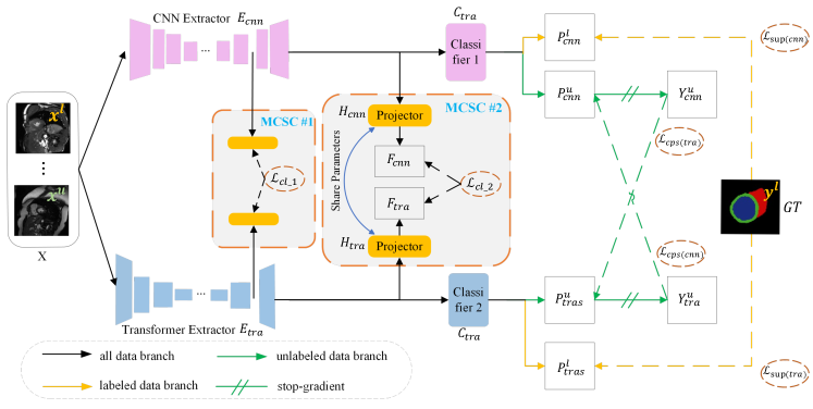
Figure 1: The overall architecture of our MCSC framework for semi-supervised segmentation. Two networks, a CNN (pink) and Transformer (blue), with complementary inductive biases, learn together. When training on unlabelled data, each network generates pseudo labels for the other. These labels are used to define a pseudo supervision loss and a novel local contrastive loss that improves the quality of representations learnt by the models.

We adopt a student–student framework based on [4], with cross-teaching between a CNN-based U-Net and a Transformer-based U-Net. This leverages the advantages of convolution-based and Transformer-based segmentation networks for learning local semantic information and long-range dependencies, and enables the two models to achieve consistency on segmentation prediction. However, this framework has some limitations: (i) it only focuses on the prediction consistency on each image slice at output level; (ii) it ignores the dissimilarity and similarity among different and same segmentation categories across the whole dataset. To overcome this, we propose a Multi-Scale Cross Supervised Contrastive Learning (MCSC) framework to pull closer the features of the same category and push away the features of different categories from both networks. It not only ensures the consistency of two models on the feature and output level, but also enhances the distinguishability of features in different categories, thereby improving the segmentation performance. We illustrate the overall architecture of our framework in Figure 1. The branch of CNN or Transformer includes a feature extractor $E_{*}(\cdot)$, a segmentation head $C_{*}(\cdot)$, and two feature space projectors $H_{*}(\cdot)$. Both branches only share the parameters of the last layer in the feature space projectors.

Given a training dataset consisting of a small labelled subset $D_{l}=\{x_{i}^{l},y_{i}^{l}\}_{i=1}^{K}$ and a large unlabelled set $D_{u}=\{x_{j}^{u}\}_{j=1}^{M}$, where $M\gg K$, the input to our model is a minibatch $X=X^{l}\cup X^{u}$ including labelled images and unlabelled images. The minibatch $X$ is first fed into the CNN-based and Transformer-based networks to obtain their feature representations and segmentation logits. In the semi-supervised setting, we employ the following supervision losses for training: (i) on the output level, we calculate the supervision loss $\mathcal{L}_{sup}$ (yellow dashed lines in Figure 1) between the segmentation predictions and the limited labelled data, as well as the cross pseudo supervision loss $\mathcal{L}_{cps}$ (green dashed lines in Figure 1) between the segmentation predictions and the pseudo labels from the CNN-based U-Net or the Transformer-based U-Net in a cross teaching manner on the output level (Section 3.1); (ii) on the feature level, we employ the proposed multi-scale cross contrastive loss $\mathcal{L}_{cl}$ (black dashed lines in Figure 1) to enhance feature consistency of the same segmentation category and feature distinguishability of the different segmentation categories across the whole dataset (labelled and unlabelled) guided by cross pseudo-supervision (Section 3.2).

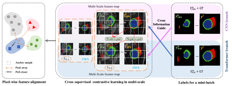
Figure 2: Multi-scale cross supervised contrastive learning. Pseudo labels from cross-teaching (right) are combined with ground-truth labels where available, and used to define a local contrastive loss over features of different scales (middle, orange dashed boxes). This contrastive pairs of pixels drawn from either the same or different slices; for efficiency it is defined over patches. Features of pixels of the same (pseudo-) class are pulled together (left), while those of different classes are pushed apart.

3.1 Cross Pseudo Supervision

The CNN and Transformer networks teach each other using the unlabelled data, through a cross pseudo supervision loss $\mathcal{L}_{cps}$ [4, 8]. This regularises their respective predictions to be consistent with each other. Specifically, the predictions made by the CNN become pseudo labels that supervise the Transformer, and vice-versa. The unlabelled images $X^{u}$ are fed into the feature extractors $E_{*}(\cdot)$ and classifier heads $C_{*}(\cdot)$ of the two models respectively, to get class probability maps $P^{u}_{*}=\mathrm{softmax}\{C_{*}(E_{*}(X^{u}))\}$, and pseudo one-hot label map $Y^{u}_{*}=\mathrm{argmax}\,(P^{u}_{*})$, where $*$ denotes the CNN or Transformer branch. We then define two consistency loss terms: $\mathcal{L}_{cps(cnn)}$ uses the Transformer’s pseudo-labels to supervise the CNN, and $\mathcal{L}_{cps(tra)}$ the reverse; these are given by:

$$\small\mathcal{L}_{cps(cnn)}=\mathcal{L}_{dice}(P^{u}_{cnn},Y^{u}_{tra}),\;\;\;\mathcal{L}_{cps(tra)}=\mathcal{L}_{dice}(P^{u}_{tra},Y^{u}_{cnn}).$$ (1)

Here $\mathcal{L}_{dice}$ is the standard Dice loss function, but using pseudo-labels instead of ground-truth segmentation. Note that during training there is no gradient back-propagation between $P^{u}_{cnn}$ and $Y^{u}_{cnn}$, and similar from $P^{u}_{tra}$ to $Y^{u}_{tra}$.

3.2 Multi-Scale Cross Supervised Contrastive Learning (MCSC)

Cross pseudo supervision does not exploit feature regularities across the whole dataset, e.g. similarity between representations of the same organ in different slices. We therefore add a contrastive loss, operating on multi-scale features extracted from the Transformer and the CNN. This has two advantages: (i) It encourages consistency of the two models’ internal features (not just outputs) (ii) It captures high-level semantic relationships between distant regions, and between features on both labelled and unlabelled data.

Our MCSC module (Figure 2) is based on local supervised contrastive learning [19], which learns a compact feature space by reducing the distance in the embedding space between positive pairs, and increasing the distance between negative pairs. Firstly, it extracts features from the CNN and Transformer, then projects them into a common embedding space. This is followed by a novel approach of selecting positive and negative pairs using the pseudo labels, and a class-balanced contrastive loss calculated on these.

Feature Embedding.

After $X=\{x_{i}\}_{i=1\cdots N}$ is passed into $E_{cnn}(\cdot)$ and $E_{tra}(\cdot)$ respectively, the resulting features are projected by passing them through projectors $H_{\mathrm{cnn}}(\cdot)$ and $H_{\mathrm{tra}}(\cdot)$ into a unified feature space, where we will sample pairs to contrast. Overall, we get a feature batch $F$ consisting of $2N$ feature maps $f_{i}=H(E(x_{i}))\in\mathbb{R}^{h\times w\times c}$, where $f_{1\ldots N}$ come from the CNN and $f_{N+1\ldots 2N}$ from the Transformer (middle of Figure 2).

Cross Supervised Sampling.

For cross supervised sampling, we follow these strategies: (i) We exchange class information from two models to guide the sampling, using the prediction of Transformer to be the supervisory information for CNN and vice-versa (Figure 2, right). This is consistent with the cross-prediction loss $\mathcal{L}_{cps}$, and implicitly it also makes the features predicted by the two models on the same slice consistent. (ii) We contrast features on both unlabelled and labelled data. Since the pseudo labels are of varying quality, labelled data is included in the contrastive loss to reduce the noise. (iii) We contrast pixels both within and between slices. Previous work focuses on inter-slice samples and ignores useful anatomical information within slices. For example, compared to different slices, the features of different class of organ boundaries in the image should be more similar. By focusing on them, we can refine the details of the hardest boundary segmentation. Therefore, our strategy differs significantly from existing approaches to sampling pairs in supervised contrastive learning with semi-supervised segmentation, where positive or negative pairs are selected based on pseudo labels on unlabelled data [23, 17, 22].

The computational complexity and memory for the supervised contrastive loss is very high; however, comparing many samples is crucial for improving the performance of contrastive learning [31]. To address this problem, inspired by [21], we compute the local contrastive loss over patches. We divide all the feature maps in $F$ into patches with size of $h^{\prime}\times h^{\prime}$. Let us assume there are $M$ patches of each $f$. We randomly select (without replacement) a patch from each feature map in $F$, and finally we get $M$ batches of $2N$ patches. The loss is evaluated on $2N$ patches from each batch in turn, until the entire $f$ has been traversed.

Balanced Supervised Local Contrastive Loss.

After sampling positive/negative pairs of pixels, a contrastive loss is introduced to pull positive pairs closer and push negative pairs apart within the $2N$ patches. Given the extreme imbalance between background and foreground (different organs), a randomly sampled batch tends to consist of a significantly larger number of positive and negative pairs for the background, compared to the foreground organs. This inherent imbalance inevitably biases conventional supervised contrastive learning towards the background, consequently neglecting the differentiation of foreground categories. Simply eliminating the background during contrastive learning [21] is not an optimal solution, as (i) the remaining number of foreground pixels is extremely small, and (ii) this fails to capture the relationship between the background and the foreground.

Inspired by [35], we average both the inter-class (positive) and intra-class (negative) feature contrast within the pixels of each class, and then forward it to calculate the supervised contrastive loss. In this way, each class makes an approximately balanced contribution. This balanced contrastive loss is implemented as follows:

$$\mathcal{L}_{bcl}=-\frac{1}{\lvert A\rvert}\sum_{a_{i}\in A}\frac{1}{\lvert A_{y}\rvert-1}\sum\limits_{p\in{A_{y}\backslash\{i\}}}\mathrm{log}\frac{\mathrm{exp}(a_{i}\cdot a_{p}/\tau)}{\sum_{j\in{Y_{A}}}\frac{1}{\lvert A_{j}\rvert}\sum\limits_{a_{k}\in{A_{j}}}\mathrm{exp}(a_{i}\cdot a_{k}/\tau)},$$ (2)

where $A$ is the pixel-level feature sets of the $2N$ patches, $a_{i}$ represents the $i^{th}$ feature, $A_{y}$ is a subset that contains all samples of class $y$, $A_{y}\backslash\{i\}$ represents all the pixels in $A_{y}$ excluding $a_{i}$, $Y_{A}$ represents the set of all the unique classes in current $A$, and $\tau$ is a temperature constant. By balancing the contribution of each class during contrastive learning, we avoid the learned representations being biased towards the dominant background. Note that $\mathcal{L}_{bcl}$ is calculated over each $2N$ patches, and then averaged over $M$ batches of $2N$ patches for back-propagation.

Multi-Scale Contrastive Loss.

Existing works on local contrastive learning pass the features of the last layer before the classifier into the projector. However, the feature maps from earlier layers focus on coarser geometric information like the shape of organs, and later feature maps on details; both are important for segmentation, which depends both on relationships among multiple organs and gross anatomic structure (global) and textures of the specific tissues (local). We therefore pass features with $n$ different scales from $n$ layers of extractors and separate projectors, and then calculate each scale balanced contrastive loss $\mathcal{L}_{bcl}$ as $\mathcal{L}_{cl\_i}$. The overall loss $\mathcal{L}_{cl}$ is given by summing over each scale loss: $\mathcal{L}_{cl}=(\mathcal{L}_{cl\_1}+\ldots+\mathcal{L}_{cl\_n})$.

3.3 Optimization

The two networks are trained to minimize a weighted sum of the losses described in the previous sections: $\scriptsize\mathcal{L}_{cnn}=\mathcal{L}_{sup(cnn)}+w_{cps}\mathcal{L}_{cps(cnn)}+w_{cl}\mathcal{L}_{cl}$ and $\scriptsize\mathcal{L}_{tra}=\mathcal{L}_{sup(tra)}+w_{cps}\mathcal{L}_{cps(tra)}+w_{cl}\mathcal{L}_{cl}$, where $w_{*}$ are weighting factors used to balance the impact of individual loss terms. $w_{cps}$ is defined by a Gaussian warming up function [4]: $w_{cps}(t_{i})=0.1\cdot e^{(-5(1-t_{i}/t_{total})^{2})}$, where $t_{i}$ is $i$^th iteration of training and $t_{total}$ is the total number of iterations, while $w_{cl}$ is set to a constant value of $10^{-3}$ based on performance of the validation. Note that the Transformer is used only during training, and does not contribute to the final inference – the CNN is less computationally expensive, but has distilled the Transformer’s knowledge.

4 Experiments

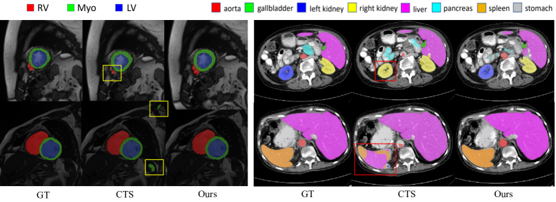
Figure 3: Qualitative results from our method and the best baseline CTS [4] trained on 4 and 7 labelled cases on ACDC (left) and Synapse (right), respectively.

We evaluate our method on two benchmark datasets, ACDC [24] and Synapse [25]. ACDC contains 200 short-axis cardiac MR images from 100 cases (i.e. patients) with masks of the left ventricle (LV), myocardium (Myo), and right ventricle (RV) to be segmented; we follow the data split and the selection of labelled cases in [4]. Synapse contains abdominal CT scans from 30 cases with eight organs including aorta, gallbladder, spleen, left kidney, right kidney, liver, pancreas and stomach; the splits follow [36]. To quantitatively assess performance, we report two popular metrics: Dice coefficient (DSC) and $95\%$ Hausdorff Distance (HD).

We implemented our method in PyTorch. We used simple data augmentations to reduce overfitting: random cropping with a $224\times 224$ patch, random flipping and rotations. All methods were trained till validation-set convergence (which was by 40,000 iterations). We selected the best checkpoint for evaluation based on validation set performance. Our method was trained using AdamW [37] with a weight decay of $5\times 10^{-4}$. We utilized the poly learning rate schedule, initialized at $5\times 10^{-4}$ for CNN and $1\times 10^{-4}$ for Transformer. The batch sizes were 4 and 10 respectively, with half labeled and half unlabeled images. For our MCSC module, each projector $H_{*}$ has two linear layers, where the first linear layer changes the dimension of feature map to 256 channels; the last layer has 128 channels and shares its parameters between the two models. In Eq.(2), temperature $\tau=0.1$. We use multi-scale feature maps from three layers of $E_{*}$, with sizes of $256\times 256$, $56\times 56$, and $28\times 28$ respectively, and the size $h^{\prime}$ of a patch was set to 19, 28 and 14 accordingly. All experiments were run on one (for ACDC) or two (for Synapse) RTX 3090 GPUs.

4.1 Comparison with Other Semi-Supervised Methods

We compare our proposed method to several recent SSL methods that use U-Net as backbone, including Mean Teacher (MT) [12], Deep Co-Training (DCT) [13], Uncertainty Aware Mean Teacher (UAMT) [14], Interpolation Consistency Training (ICT) [38], Cross Consistency Training (CCT) [39], Cross Pseudo Supervision (CPS) [8], and the state-of-the-art (SOTA) method Cross Teaching Supervision (CTS) [4]. Results for the weaker methods MT, DCT and ICT are given in the supplementary material. We also compare against a U-Net trained with full supervision (UNet-FS), and one trained only on the labelled subset of data (UNet-LS). Finally we compare with the SOTA fully-supervised Transformer based methods BATFormer [40] on ACDC, and nnFormer [41] on Synapse. We retrained all the semi-supervised baselines using their original settings (optimizer and batch size), and report whichever is better of our retrained model or the result quoted in [4].

Results on ACDC.

Table 1 shows evaluation results of MCSC and the best-performing baseline under three different levels of supervision (7, 3 and 1 labelled cases). Our MCSC method trained on $10\%$ of cases improves both DSC and HD metrics compared to previous best SSL methods by a significant margin (more than $3\%$ on DSC and 5mm on HD). More importantly, it achieves 2.3mm HD, significantly better than even the fully supervised U-Net and BATFormer, which achieve 4.0 and 8.0 respectively. It also demonstrates competitive DSC of 89.4 $\%$, compared with 91.7 $\%$ and 92.8 $\%$ of U-Net and BATFormer. In addition, MCSC performance is highly resilient to the reduction of labelled data from $10\%$ to $5\%$, outperforming the previous SOTA SSL methods by around $10\%$ on DSC. The improvement is even more profound for the minority and hardest class, RV, with performance gains of 14 $\%$ on DSC and 13.6mm on HD. Figure 3 shows qualitative results from UNet-LS, CPS, CTS and our method. MCSC produces a more accurate segmentation, with fewer under-segmented regions on minority class- RV (top) and fewer false-positive (bottom). Overall, results prove that MCSC improving the semantic segmentation capability on unbalanced and limited-annotated medical image dataset by a large margin.

Labelled	Methods	Mean		Myo		LV		RV
		DSC$\uparrow$	HD$\downarrow$	DSC$\uparrow$	HD$\downarrow$	DSC$\uparrow$	HD$\downarrow$	DSC$\uparrow$	HD$\downarrow$
70 cases (100$\%$)	UNet-FS	91.7	4.0	89.0	5.0	94.6	5.9	91.4	1.2
	BATFormer [40]	92.8	8.0	90.26	6.8	96.30	5.9	91.97	11.3
7 cases (10$\%$)	UNet-LS	75.9	10.8	78.2	8.6	85.5	13.0	63.9	10.7
	CCT [39]	84.0	6.6	82.3	5.4	88.6	9.4	81.0	5.1
	CPS [8]	85.0	6.6	82.9	6.6	88.0	10.8	84.2	2.3
	CTS [4]	86.4	8.6	84.4	6.9	90.1	11.2	84.8	7.8
	MCSC (Ours)	89.4	2.3	87.6	1.1	93.6	3.5	87.1	2.1
3 cases (5$\%$)	UNet-LS	51.2	31.2	54.8	24.4	61.8	24.3	37.0	44.4
	CCT [39]	58.6	27.9	64.7	22.4	70.4	27.1	40.8	34.2
	CPS [8]	60.3	25.5	65.2	18.3	72.0	22.2	43.8	35.8
	CTS [4]	65.6	16.2	62.8	11.5	76.3	15.7	57.7	21.4
	MCSC (Ours)	73.6	10.5	70.0	8.8	79.2	14.9	71.7	7.8
1 case	UNet-LS	26.4	60.1	26.3	51.2	28.3	52.0	24.6	77.0
	CTS [4]	46.8	36.3	55.1	5.5	64.8	4.1	20.5	99.4
	MCSC (Ours)	58.6	31.2	64.2	13.3	78.1	12.2	33.5	68.1
Best is reported as bold, Second Best is underlined.

Table 1: Segmentation results on DSC($\%$) and HD(mm) of our method and baselines on ACDC, across different numbers of labelled cases.

Results on Synapse.

Table 2 shows the segmentation results of the best-performing baselines on Synapse with 4 and 2 labelled cases. Compared to ACDC, Synapse is a more challenging segmentation benchmark as it includes a larger number of labelled regions with far more imbalanced volumes. Nevertheless, our method outperforms the baselines by a large margin. This demonstrates the robustness of our proposed framework, and the benefit of regularising multi-scale features from two models to be semantically consistent across the whole dataset. This is further highlighted in the qualitative results provided in Figure 3.

Labelled	Methods	DSC$\uparrow$	HD$\downarrow$	Aorta	Gallb	Kid$\_$L	Kid$\_$R	Liver	Pancr	Spleen	Stom
18 cases(100 $\%$)	UNet-FS	75.6	42.3	88.8	56.1	78.9	72.6	91.9	55.8	85.8	74.7
	nnFormer [41]	86.6	10.6	92.0	70.2	86.6	86.3	96.8	83.4	90.5	86.8
4 cases(20 $\%$)	UNet-LS	47.2	122.3	67.6	29.7	47.2	50.7	79.1	25.2	56.8	21.5
	CCT [39]	51.4	102.9	71.8	31.2	52.0	50.1	83.0	32.5	65.5	25.2
	CPS [8]	57.9	62.6	75.6	41.4	60.1	53.0	88.2	26.2	69.6	48.9
	CTS [4]	64.0	56.4	79.9	38.9	66.3	63.5	86.1	41.9	75.3	60.4
	MCSC (Ours)	66.8	28.2	75.2	37.2	73.1	71.5	92.4	41.0	86.1	57.8
2 cases(10 $\%$)	UNet-LS	45.2	55.6	66.4	27.2	46.0	48.0	82.6	18.2	39.9	33.4
	CCT [39]	46.9	58.2	66.0	26.6	53.4	41.0	82.9	21.2	48.7	35.6
	CPS [8]	48.8	65.6	70.9	21.3	58.0	45.1	80.7	23.5	58.0	32.7
	CTS [4]	52.0	63.7	73.2	12.7	67.2	64.7	82.9	31.7	40.9	42.4
	MCSC (Ours)	55.8	25.9	72.6	20.4	73.8	71.3	91.0	3.5	75.4	38.6
Best is reported as bold, Second Best is underlined.

Table 2: Comparison with different models on Synapse. The performance is reported by class-mean DSC (%) and HD (mm), as well as the DSC value for each organ.

4.2 Ablation study

In Table 4 we explore the influence of proposed modules on the performance on ACDC with 7 labelled cases. Starting from CTS [4] (top row), and adding supervised local contrastive learning (SCL) with a prior approach for balancing the loss (DB [21]), we observe a significant improvement of $1.1\%$ on DSC; this emphasizes the importance of enforcing consistency between features of the two models. By exchanging class information from CNN and Transformer to select contrasted samples (instead of using each model’s own predictions as pseudo-labels), we see an improvement in DSC and HD from 87.50 to 88.23 and 7.4 to 3.4 respectively. Our approach to balancing different classes (Balanced), instead of just discarding background pixels (DB), improves DSC by 0.7%, since minority classes are better separated. Finally, utilizing multi-scale instead of just final-layer features further improves performance by 0.58% and 2.3% DSC and HD respectively.

In Table 4, we compare results using different feature maps as input to the contrastive loss; we see best performance is achieved by using both $256\times 256$ and $28\times 28$ feature maps. Thus, combining coarser geometric information in global features and detailed local features does indeed benefit medical image segmentation.

SCL	DB	CroLab	Balanced	MulSca	DSC$\uparrow$	HD$\downarrow$
					86.40	8.6
✓	✓				87.50	7.4
✓	✓	✓			88.23	3.4
✓		✓	✓		88.80	4.6
✓		✓	✓	✓	89.38	2.3

Table 3: Ablation study for the primary components of our model. SCL denotes supervised local contrastive loss. DB denotes discarding background pixels as anchor. CroLab stands for cross label information of two models to select contrastive sample. Balanced means averaging the instances of each class in denominator of SCL. MulSca means contrasting multi-scale feature maps.

Branches			Mean
256	56	28	DSC$\uparrow$	HD$\downarrow$
✓			88.80	4.6
	✓		88.88	4.2
		✓	88.39	4.5
✓		✓	89.38	2.3
✓	✓		88.92	2.9
✓	✓	✓	88.35	4.3

Table 4: Ablation analysis on the choice of feature maps for the multi-scale contrastive loss (ACDC, 7 labelled cases). Full table is in the supplementary material.  

4.3 Visualization of features with contrastive learning

Figure 4 shows visualizations of embedding features applying t-SNE on a single slice of two cases from the test data of ACDC and Synapse respectively. The models are trained with 7 cases (ACDC) and 4 cases (Synapse). Different colors represent different classes. Features are taken from the feature map after the projector with scale of $256\times 256$, and each point in the figure is the embedding of one pixel. The standard SCL is the second row of Table 3 in the main text (SCL+DB). For ACDC, the left case 1 shows our method better separates RV from the other two foreground classes, and reduces the overlap between LV and Myo. For the case 2, the foreground clusters of ours are tighter. A more clear and consistent effect can be seen on Synapse. For the case on the left, our method makes the liver, spleen and stomach much better separated than standard SCL. A similar situation also occurs with the left and right kidneys for the case 2. Overall, through cross labelling, averaging the contribution of each class in SCL, and contrasting multi-scale feature maps, our method obtains a better embedding representations for segmentation, where features within the same class are pulled closer and features for different class are spread farther apart.

Figure 4: Visualization of embedding features from our method and standard SCL after applying t-SNE on test data of ACDC and Synapse respectively. Each case represents one slice from a different patient.

5 Conclusion

We have presented a novel SSL framework for medical image segmentation based on cross-teaching between a Transformer and a CNN. This incorporates a supervised local contrastive loss, named MCSC, that encourages intra-class feature similarity and inter-class discriminativity across the whole dataset. Furthermore, it addresses class imbalance with a loss that eliminates the negative effects of excessive background pixels. Finally, it contrasts multi-scale feature maps, to combine global and local feature understanding. Our experiments on two commonly used medical datasets demonstrate that the proposed framework can fully take advantage of labelled and unlabelled data, and demonstrates remarkably resiliant performance even when the labelled data are significantly reduced.

6 Acknowledgements

The authors acknowledge funding by China Scholarship Council, EPSRC (EP/W01212X/1) and Royal Society (RGS/R2/212199).

References

- [1] Chen Chen et al. “Deep learning for cardiac image segmentation: a review” In Frontiers in Cardiovascular Medicine 7 Frontiers Media SA, 2020, pp. 25
- [2] Dinggang Shen, Guorong Wu and Heung-Il Suk “Deep learning in medical image analysis” In Annual review of biomedical engineering 19 Annual Reviews, 2017, pp. 221–248
- [3] Nima Tajbakhsh et al. “Embracing imperfect datasets: A review of deep learning solutions for medical image segmentation” In Medical Image Analysis 63 Elsevier, 2020, pp. 101693
- [4] Xiangde Luo et al. “Semi-supervised medical image segmentation via cross teaching between cnn and transformer” In International Conference on Medical Imaging with Deep Learning, 2022, pp. 820–833 PMLR
- [5] Yuanyi Zhong et al. “Pixel contrastive-consistent semi-supervised semantic segmentation” In Proceedings of the IEEE/CVF International Conference on Computer Vision, 2021, pp. 7273–7282
- [6] Yassine Ouali, Celine Hudelot and Myriam Tami “Semi-supervised semantic segmentation with cross-consistency training” In Proceedings of the IEEE/CVF Conference on Computer Vision and Pattern Recognition, 2020, pp. 12674–12684
- [7] Constantin Marc Seibold, Simon Reiß, Jens Kleesiek and Rainer Stiefelhagen “Reference-Guided Pseudo-Label Generation for Medical Semantic Segmentation” In The Thirty-Sixth AAAI Conference on Artificial Intelligence, 2022, pp. 2171–2179
- [8] Xiaokang Chen, Yuhui Yuan, Gang Zeng and Jingdong Wang “Semi-supervised semantic segmentation with cross pseudo supervision” In Proceedings of the IEEE/CVF Conference on Computer Vision and Pattern Recognition, 2021, pp. 2613–2622
- [9] Yingda Xia et al. “3D Semi-Supervised Learning with Uncertainty-Aware Multi-View Co-Training” In Proceedings of the IEEE/CVF Conference on Computer Vision and Pattern Recognition, 2020, pp. 3646–3655
- [10] Kaiping Wang et al. “Semi-supervised medical image segmentation via a tripled-uncertainty guided mean teacher model with contrastive learning” In Medical Image Analysis 79 Elsevier, 2022, pp. 102447
- [11] J. Yang et al. “Self-supervised sequence recovery for semi-supervised retinal layer segmentation” In IEEE Journal of Biomedical and Health Informatics, 2022, pp. 3872–3883 IEEE
- [12] Antti Tarvainen and Harri Valpola “Mean teachers are better role models: Weight-averaged consistency targets improve semi-supervised deep learning results” In Advances in neural information processing systems 30, 2017
- [13] Siyuan Qiao et al. “Deep co-training for semi-supervised image recognition” In Proceedings of the european conference on computer vision (eccv), 2018, pp. 135–152
- [14] Lequan Yu et al. “Uncertainty-aware self-ensembling model for semi-supervised 3D left atrium segmentation” In Medical Image Computing and Computer Assisted Intervention–MICCAI 2019: 22nd International Conference, Shenzhen, China, October 13–17, 2019, Proceedings, Part II 22, 2019, pp. 605–613 Springer
- [15] Xinlei Chen and Kaiming He “Exploring simple siamese representation learning” In Proceedings of the IEEE/CVF conference on computer vision and pattern recognition, 2021, pp. 15750–15758
- [16] Prannay Khosla et al. “Supervised Contrastive Learning” In Advances in Neural Information Processing Systems 33 Curran Associates, Inc., 2020, pp. 18661–18673 URL: https://proceedings.neurips.cc/paper_files/paper/2020/file/d89a66c7c80a29b1bdbab0f2a1a94af8-Paper.pdf
- [17] Huisi Wu et al. “Cross-patch dense contrastive learning for semi-supervised segmentation of cellular nuclei in histopathologic images” In Proceedings of the IEEE/CVF Conference on Computer Vision and Pattern Recognition, 2022, pp. 11666–11675
- [18] Krishna Chaitanya, Ertunc Erdil, Neerav Karani and Ender Konukoglu “Contrastive learning of global and local features for medical image segmentation with limited annotations” In Advances in Neural Information Processing Systems 33, 2020, pp. 12546–12558
- [19] Wenguan Wang et al. “Exploring cross-image pixel contrast for semantic segmentation” In Proceedings of the IEEE/CVF International Conference on Computer Vision, 2021, pp. 7303–7313
- [20] Zeju Li, Konstantinos Kamnitsas and Ben Glocker “Analyzing overfitting under class imbalance in neural networks for image segmentation” In IEEE transactions on medical imaging 40.3 IEEE, 2020, pp. 1065–1077
- [21] Xinrong Hu, Dewen Zeng, Xiaowei Xu and Yiyu Shi “Semi-supervised contrastive learning for label-efficient medical image segmentation” In Medical Image Computing and Computer Assisted Intervention–MICCAI 2021: 24th International Conference, Strasbourg, France, September 27–October 1, 2021, Proceedings, Part II 24, 2021, pp. 481–490 Springer
- [22] Krishna Chaitanya, Ertunc Erdil, Neerav Karani and Ender Konukoglu “Local contrastive loss with pseudo-label based self-training for semi-supervised medical image segmentation” In Medical Image Analysis 87 Elsevier, 2023, pp. 102792
- [23] Xiangyu Zhao et al. “RCPS: Rectified Contrastive Pseudo Supervision for Semi-Supervised Medical Image Segmentation” In arXiv preprint arXiv:2301.05500, 2023
- [24] Olivier Bernard et al. “Deep learning techniques for automatic MRI cardiac multi-structures segmentation and diagnosis: is the problem solved?” In IEEE transactions on medical imaging 37.11 ieee, 2018, pp. 2514–2525
- [25] Bennett Landman et al. “Miccai multi-atlas labeling beyond the cranial vault–workshop and challenge” In Proc. MICCAI Multi-Atlas Labeling Beyond Cranial Vault—Workshop Challenge 5, 2015, pp. 12
- [26] Jizong Peng, Guillermo Estrada, Marco Pedersoli and Christian Desrosiers “Deep co-training for semi-supervised image segmentation” In Pattern Recognition 107 Elsevier, 2020, pp. 107269
- [27] Gerda Bortsova et al. “Semi-supervised medical image segmentation via learning consistency under transformations” In Medical Image Computing and Computer Assisted Intervention–MICCAI 2019: 22nd International Conference, Shenzhen, China, October 13–17, 2019, Proceedings, Part VI 22, 2019, pp. 810–818 Springer
- [28] Ting Chen, Simon Kornblith, Mohammad Norouzi and Geoffrey Hinton “A simple framework for contrastive learning of visual representations” In International conference on machine learning, 2020, pp. 1597–1607 PMLR
- [29] Jean-Bastien Grill et al. “Bootstrap your own latent-a new approach to self-supervised learning” In Advances in neural information processing systems 33, 2020, pp. 21271–21284
- [30] Yuandong Tian, Xinlei Chen and Surya Ganguli “Understanding self-supervised learning dynamics without contrastive pairs” In International Conference on Machine Learning, 2021, pp. 10268–10278 PMLR
- [31] Kaiming He et al. “Momentum contrast for unsupervised visual representation learning” In Proceedings of the IEEE/CVF conference on computer vision and pattern recognition, 2020, pp. 9729–9738
- [32] Zhenda Xie et al. “Propagate yourself: Exploring pixel-level consistency for unsupervised visual representation learning” In Proceedings of the IEEE/CVF Conference on Computer Vision and Pattern Recognition, 2021, pp. 16684–16693
- [33] Xinlong Wang et al. “Dense contrastive learning for self-supervised visual pre-training” In Proceedings of the IEEE/CVF Conference on Computer Vision and Pattern Recognition, 2021, pp. 3024–3033
- [34] Fan Yang et al. “Class-aware contrastive semi-supervised learning” In Proceedings of the IEEE/CVF Conference on Computer Vision and Pattern Recognition, 2022, pp. 14421–14430
- [35] Jianggang Zhu et al. “Balanced contrastive learning for long-tailed visual recognition” In Proceedings of the IEEE/CVF Conference on Computer Vision and Pattern Recognition, 2022, pp. 6908–6917
- [36] Jieneng Chen et al. “Transunet: Transformers make strong encoders for medical image segmentation” In arXiv preprint arXiv:2102.04306, 2021
- [37] Ilya Loshchilov and Frank Hutter “Decoupled weight decay regularization” In arXiv preprint arXiv:1711.05101, 2017
- [38] Vikas Verma et al. “Interpolation consistency training for semi-supervised learning” In Neural Networks 145 Elsevier, 2022, pp. 90–106
- [39] Yassine Ouali, Céline Hudelot and Myriam Tami “Semi-supervised semantic segmentation with cross-consistency training” In Proceedings of the IEEE/CVF Conference on Computer Vision and Pattern Recognition, 2020, pp. 12674–12684
- [40] Xian Lin, Li Yu, Kwang-Ting Cheng and Zengqiang Yan “BATFormer: Towards Boundary-Aware Lightweight Transformer for Efficient Medical Image Segmentation” In IEEE Journal of Biomedical and Health Informatics IEEE, 2023
- [41] Hong-Yu Zhou et al. “nnformer: Interleaved transformer for volumetric segmentation” In arXiv preprint arXiv:2109.03201, 2021