Many-species ecological fluctuations as a jump process from the brink of extinction

Abstract

Highly-diverse ecosystems exhibit a broad distribution of population sizes and species turnover, where species at high and low abundances are exchanged over time. We show that these two features generically emerge in the fluctuating phase of many-variable model ecosystems with disordered species interactions, when species are supported by migration from outside the system at a small rate. We show that these and other phenomena can be understood through the existence of a scaling regime in the limit of small migration, in which large fluctuations and long timescales emerge. We construct an exact analytical theory for this asymptotic regime, that provides scaling predictions on timescales and abundance distributions that are verified exactly in simulations.

In this regime, a clear separation emerges between rare and abundant species at any given time, despite species moving back and forth between the rare and abundant subsets. The number of abundant species is found to lie strictly below a well-known stability bound, maintaining the system away from marginality. At the same time, other measures of diversity, which also include some of the rare species, go above this bound.

In the asymptotic limit where the migration rate goes to zero, trajectories of individual species abundances are described by non-Markovian jump-diffusion processes, which proceeds as follows: A rare species remains so for some time, then experiences a jump in population sizes after which it becomes abundant (a species turnover event) and later sees its population size gradually decreasing again until rare, due to the competition with other species. The asymmetry of abundance trajectories under time-reversal is maintained at small but finite migration rate. These features may serve as fingerprints of endogenous fluctuations in highly-diverse ecosystems.

I Introduction

In ecological communities, interactions between species can drive changes in population sizes. For few-species communities, experiments find dynamics including stable equilibria, periodic oscillations and chaos [1, 2, 3], which are explained in terms of dynamical models of interacting populations, such as Lotka-Volterra or resource-competition models [4]. Yet many natural ecosystems, from microbes in a grain of soil to plants in a rainforest, can be staggeringly diverse. Nevertheless, the dynamics of such highly-diverse communities are far less understood.

Observations on highly diverse systems show that the distribution of species abundances (population sizes) at a given time is often very broad, with many species at very low population size [5, 6]. Time fluctuations in abundances can be very large, with “blooms” and significant species turnover, where the species at high and low abundances are exchanged over time [7, 8, 9].

Theoretically, dynamical models of interacting populations with many variables can be notoriously challenging to analyze. They are parameterized by very many parameters describing the interactions between species, which are unknown and often unrealistic to obtain from measurements. This has prompted a change of paradigm (following similar ideas in physics and other fields), replacing unknown parameters by randomly sampled ones [10, 11], and looking for typical and universal properties of the many-variable systems. Both physicists and ecologists aim to classify the different broad behaviors and the robust features of each, formalized within physics as “phases”. An important contribution of statistical physics is the ability to provide mathematical frameworks, giving systematic answers to questions on these robust properties. This work provides such a framework for one such challenging phase.

Two distinct phases that have recently attracted much attention, are a phase where the abundances of different species reach a fixed point, and another where they fluctuate indefinitely [12, 13]. These distinct behaviors have been observed in controlled experiments where properties of microbial communities are varied [14], highlighting the power of robust theoretical predictions when applied to ecological phenomena.

Most of the theoretical work so far has been devoted to the fixed point phase, and many of its properties are well understood, including the abundance distribution, and limits on the fixed point stability that signal the transition to the fluctuating phase [12, 13, 15]. Predictions obtained theoretically for the fixed-point phase stand in contrast with empirically observed broad abundance distributions, and are also unable to account for situations where large abundance fluctuations are observed. The dynamical phase, which is the focus of this work, holds promise of addressing these limitations.

Much less has been known about the dynamical phase. For well-mixed systems (no explicit space), that are coupled to the outside by a migration of all species, simulations have shown that the system reached a stationary chaotic state [16]. Similar results have been obtained from simulations of coupled spatial locations [17, 18]. However, for well-mixed systems in the absence of migration, a dynamical slowdown is observed, along with large population fluctuations [16, 18]. Analytical results for many-species fluctuating dynamics have been derived when interactions are fully anti-symmetric, in which case a stationary chaotic state is reached even without migration [18]. Yet, this state is sensitive to the anti-symmetry that is not expected to hold generally in nature [18]. A few-species model featuring dynamical slowdown and large fluctuations is the three-species rock-paper-scissors dynamics, cycling between and ever-closer to three unstable fixed points (a heteroclinic orbit) [19]. This elegant model serves as an instructive analogy for many-species dynamics [18, 20, 21], yet is only of limited relevance to many-species properties such as diversity, abundance distributions, and stability. A many-species exactly-solvable dynamical toy model that features dynamical slowdown was introduced in [21]. Yet due to its special structure, this model did not include key features of ecological systems. In particular, questions relating diversity and linear stability that appear in many other systems cannot be addressed, and it also did not include migration that interrupts the dynamical slowdown process.

In this work, we provide a systematic analytical framework for the dynamical phase, for the Lotka-Volterra model with randomly sampled interactions, in the limit of many species, and when migration rates are small. In this phase, fluctuations in population sizes are caused solely by interactions between species, without changes in the environment. We show that it is precisely in the limit of low migration, where fluctuations in population sizes get slower and larger, that many of the striking signatures of this phase emerge. These features, which are now listed, include commonly observed traits of high-diversity natural ecosystems, such as a broad abundance distribution and species turnover, see points 1 and 2 below. In addition, they shed new light on the definition and measurement of diversity when species turnover is involved, see point 4, and uncover new phenomena that could be used as fingerprints of endogenous fluctuations, see point 5.

1. At any given time, abundances are broadly distributed, with many rare species with population size close to the minimal value set by the migration and many species with small population sizes but yet much larger than the minimal one. We show analytically that over this intermediate range, the abundance distribution scales as a power law with exponent $-1$ and characterize the corrections to this power law behavior when the migration rate is finite. Broad distributions have been measured in natural ecosystems [22, 6], but their form and origin have been debated [23, 5]. In contrast, in the fixed point phase, the number of species in this intermediate range is small and the abundances are not broadly distributed [13].

2. The dynamics exhibit species turnover, where the species at high abundance are exchanged over time with species that were at low abundances. In particular, we show that there are always species at low abundances that are able to grow. This is in contrast to the fixed point phase, where rare species cannot invade.

3. A long timescale emerges, possibly extending over many generations: as the migration gets lower, temporal changes in both abundances and growth rates become slower. This timescale scales as the absolute value of the logarithm of the migration rate, a prediction that might be directly tested in controlled experiments. Understanding the various timescales involved is key to understanding ecological dynamics [24] and this work identifies a new collective mechanism through which long timescales are robustly self-generated by species interactions in highly-diverse model ecosystems. The combination of species that can invade and long timescales allows even for species that are very rare to reach high abundance later. Hence, rare species at a given time can be important in the future, and the distinction of rare versus abundant species is not fixed in time. Due to the long timescale, the species at high abundance lie close to a fixed point, which would have been stable in the absence of the other species.

4. How do many species coexist in highly-diverse ecosystems is one of the key questions in ecology. Turnover events and broad abundance distributions raise questions as to how one might even define diversity. We show that while the list of abundant species changes in time, the fraction above any given threshold abundance fluctuates only by a little. Furthermore, in the low migration limit, the number of species with high and intermediate abundance is well-defined, namely insensitive to the precise choice of the thresholds. Finally, we show that the number of high-abundance species, which lie close to a fixed point, is strictly below the stability bound (known as the “May bound” [11]). Equivalently, this fixed point is fully stable (as opposed to marginally-stable). In contrast, the number of high-abundance and intermediate-abundance species together is not constrained by the stability bound and exceeds it. Therefore measures of species-richness that also probe the power law region of the species abundance distribution are not constrained by May’s stability bound. In fact, most of the species whose population sizes are well above the minimal value set by migration, have small abundances.

5. Lastly, we show that “bloom” dynamics, where a species grows from rare to abundant, until eventually going back to rare, are strongly asymmetric under time-reversal: The trajectory of the population size starts with a quick increase and decreases back gradually. This is an interesting signature of purely endogenous fluctuations in high-diversity ecosystems that could be looked for in empirical time series.

In addition to the above predictions, we also consider isolated systems (namely, without migration from the outside) and show that there, the timescale and size of the abundance fluctuations will continue to grow in time indefinitely. This will inevitably lead to extinctions of many species, once the finite size of the populations is taken into account.

The core of our argument is built on identifying the appropriate transformations of time and abundances, for which all dynamical properties (including steady-state distributions and two-time correlations) collapse for different values of migration, when migration is low. These scaling relations are verified exactly in collapse of simulation data. We obtain a well-defined stochastic process for these transformed variables in the limit of small but positive migration rate. The resulting picture has features that set it apart from generic many-variable chaotic dynamics. First, abundances follow non-Markovian jump-diffusion dynamics. Second, even though the dynamics are slow, the system is maintained strictly away from marginality, in contrast with glassy systems [25, 26]. Last, the emergence of the long timescale results from dynamical slowdown (aging) that would have continued indefinitely at zero migration. Yet, this slowdown is not due to the existence of a rough landscape. We trace all the unique phenomenology back to the possibility of extinctions in the absence of migration. In other words, this is a consequence of the multiplicative nature of the dynamics, which are constrained to positive population sizes with absorbing boundaries at zero population sizes.

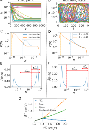
Figure 1: Species richness and species abundance distributions at fixed points (left column) and a persistently fluctuating state (right column). (A) Dynamics reaching a fixed point. (B) Persistent dynamics, where the abundances fluctuate indefinitely in the range $\lambda\lesssim N_{i}\lesssim 1$. (C-F) The corresponding distributions for $N$ and $\ln N$, denoted by $P(N)$ and $\hat{P}(\ln N)$ respectively. The distributions contain three parts (see E,F): a top part, which remains $O\left(\lambda^{0}\right)$ when $\lambda\to 0^{+}$, containing $S_{\text{top}}^{*}$ species; an intermediate part, at $\lambda\ll N\ll 1$; and a low part at $O(\lambda)$. The intermediate part contains a finite fraction of the species in the dynamical phase, but not in the fixed point phase. (G) The three definitions of species richness, normalized by $\text{var}(\alpha)$ so that $1$ is the fixed-point stability bound, as a function of the interaction variability $\sigma$. For $\sigma<\sigma_{c}$ a fixed point is reached, all three definitions coincide and lie below the stability bound, and agree with known theory (solid line). At $\sigma=\sigma_{c}$ the stability bound is reached. Beyond it, there are persistent fluctuations, and the three definitions no longer coincide: $S_{\mathrm{top}}^{*}$ is lower than the stability bound, while $S_{\mathrm{inter}}^{*}$ and $S_{\text{growth}}^{*}$ are above it. The diversities are obtained by solving the rescaled dynamics defined in Sec. IV, and agree quantitatively with careful analysis of the full equations of motion (see Sec. VII). Simulation parameters for all figures are given in Appendix 13.

II Model definition, the two phases

We start with the Lotka-Volterra system of equations

$$\dot{N}_{i}=N_{i}\left(1-N_{i}-\sum_{j(\neq i)}\alpha_{ij}N_{j}\right)+\lambda\,,$$ (1)

for $i=1\dots S$ where $S$ is the total number of species. The variables $N_{i}$ represent the abundances (population sizes) of the different species, and so $N_{i}\geq 0$ at the initial time and is guaranteed to remain so throughout. $\lambda\geq 0$ represents migration from an external source, which for simplicity is taken to be the same for all $i$.

Eq. (1) is a standard rescaling [27, 28, 13, 29] of the Lotka-Volterra equation $\dot{n}_{i}=r_{i}n_{i}/k_{i}(k_{i}-\sum_{j}A_{ij}n_{j})+D_{i}$. For simplicity, we take all $r_{i}=r$. Eq. (1) is obtained by rescaling time by $r$, and introducing the non-dimensional parameters $N_{i}\equiv n_{i}/k_{i}$, $\alpha_{ij}\equiv A_{ij}k_{j}/k_{i}$ and $\lambda\equiv D_{i}/\left(rk_{i}\right)$. Below we study the limit $\lambda\ll 1$, but assume that absolute population sizes $n_{i}$, whose minimal size is around $D_{i}/r$, are always large enough so that demographic stochasticity can be neglected. The large parameter $\left|\ln\lambda\right|$ will play an important role in the following, and since the absolute population sizes $k_{i}$ can be large (e.g., up to $10^{10}$ bacterial cells in one milliliter), $\left|\ln\lambda\right|$ can be reasonably large in ecologically relevant settings.

The limit of large $S$ is relevant to many natural high-diversity ecosystems, with hundreds to thousands of species, in communities from microbes to trees [30, 5]. We assume that $\mathbb{\alpha}$ is a random matrix with Gaussian entries, and for mathematical convenience we carry most of the analysis in the case where the interaction coefficients are all sampled independently from each other such that $\langle\alpha_{ij}\rangle=\mu/S$ and $\langle\alpha_{ij}\alpha_{kl}\rangle-\langle\alpha_{ij}\rangle\langle\alpha_{kl}\rangle=\sigma^{2}\delta_{ik}\delta_{kl}/S$. By using combinations of numerical simulations and analytical calculations, we later show that the qualitative picture presented in this paper is nonetheless robust to the addition of correlations (positive or negative) of the interaction coefficients within pairs of species, see Sec. VII .

The system exhibits different dynamical behaviors depending on the parameters [13]. When $\mu>0$ and the heterogeneity of interactions is smaller than a critical value $\sigma<\sigma_{c}$ the dynamics reach a fixed point, see Fig. 1(A). In it, some species are absent and others remain present. This definition is straightforward when $\lambda=0$, where a fixed point $dN_{i}/dt=0$ in Eq. (1) implies either $N_{i}=0$ that are the absent species, or $N_{i}>0$ which are the present species. At the stable fixed point reached, the extinct species have negative growth rates $\dot{N}_{i}/N_{i}<0$ and so cannot invade, and the subset of present species is linearly stable. For small $\lambda>0$, the absent species are now at values $N_{i}$ of order $\lambda$ and the present species are unaffected by the small $\lambda$. The requirements for a stable fixed point remain the same.

Above $\sigma>\sigma_{c}$, the system evolves indefinitely, see Fig. 1(B), without ever settling at a stable fixed point (in fact, such stable, uninvadable fixed points do not exist [31]).

III Phenomenology

We now describe key features of the dynamics when $\sigma\geq\sigma_{c}$ and $\lambda\ll 1$, starting with the Species Abundance Distribution (SAD), and then turn to the dynamics.

III.1 Species abundance and stability

The species abundance distribution $P(N)$ in the dynamically-fluctuating phase is shown in Fig. 1(D,F). It spans many orders of magnitude, ranging from $O(1)$ population sizes to order $O(\lambda)$ populations sizes. This is indeed the order of magnitude of the minimal value allowed by migration, which we call the migration floor in the following. Compared to the equilibrium situation, Fig. 1(C,E), there are many more species with abundances in the intermediate range $\lambda\ll N\ll 1$ and the fraction of species there remains finite even for small $\lambda$, see Fig. 1(F). In this range, $P(N)$ appears to be approximately a power law. The value of $P(\ln N)$ changes slowly, so the distribution of the abundances, $P(N)$, is expected to behave roughly as $N^{-1}$ [18, 32], see Fig. 1(C). In Sec. V.2, we show that in the $\lambda\to 0^{+}$ limit the power law is indeed exactly $N^{-1}$, and refine this picture with precise corrections to this $N^{-1}$ behavior.

A common way to define the number of present species (the “species richness”) is by those whose abundance lies above some value. We consider two definitions based on this idea, and an additional criterion based on the invasion growth rate. The three proposed definitions of species richness are as follows:

1. $S_{\text{top}}^{*}$ is the number of species belonging to the right peak in Fig. 1(F). Their abundance $N_{i}$ remains finite even for small $\lambda$. These are the top or abundant species.

2. $S_{\text{inter}}^{*}$ includes the number of “intermediate” species. It is all species except those belonging to the left peak in Fig. 1(F). They satisfy $N_{i}\gg\lambda$.

3. A third definition, $S_{\text{growth}}^{*}$, can be obtained through invasion experiments. If the population size of species $i$ is set to a value that is small but well-above the migration floor, $\lambda\ll N_{i}^{\mathrm{new}}\ll 1$, and keeping all other $N_{j}$ unchanged, species $i$ will grow with $\left[\dot{N}_{i}/N_{i}\right]_{\text{invasion}}=g_{i}>0$. $g_{i}$ is called the “invasion growth rate” (see, e.g. [33, 34]). For the dynamics Eq. (1), $g_{i}=1-\sum_{j(\neq i)}\alpha_{ij}N_{j}$. $S_{\text{growth}}^{*}$ counts the number of species with positive growth rate.

At the fixed point phase, all three definitions coincide, $S_{\text{top}}^{*}=S_{\text{inter}}^{*}=S_{\text{growth}}^{*}=S^{*}$, when $\lambda$ is small. In the fluctuating phase, given the presence of species in the range $\lambda\ll N\ll 1$, one might worry that species richness $S_{\text{top}}^{*}$ is not well-defined, in that it relies on an arbitrary cutoff on the abundances to decide which species are “present” or “absent”, with a similar concern for $S_{\text{inter}}^{*}$. In the limit $\lambda\to 0^{+}$, we show below that the peaks in see Fig. 1(F) become narrow compared to $\left|\ln\lambda\right|$, and therefore the definitions for $S_{\text{top}}^{*},S_{\text{inter}}^{*}$ become sharp. Focusing on $S_{\text{top}}^{*}$, we argue in Sec. VII that for $\lambda$ small but reasonable for ecological applications, these quantities can be measured in practice, and are not far from their asymptotic values.

The values of $S_{\text{top}}^{*},S_{\text{inter}}^{*},S_{\text{growth}}^{*}$ are plotted in Fig. 1(G). They are compared to a bound on species richness coming from linear stability (horizontal dashed line): If a subset of $S^{*}$ abundant species is at a fixed point, meaning that the abundances satisfy $1-N_{i}-\sum_{j(\neq i)}\alpha_{ij}N_{j}=0$, this fixed point will typically be linearly stable (ignoring other species) if $S^{*}\mathrm{var}(\alpha)\leq 1$ [11, 13]. In the fixed point phase, it is known that $S^{*}\mathrm{var}(\alpha)<1$ up to the transition [13]; thus, the stability bound is not saturated in this phase. As shown in Fig. 1(G), after crossing the transition, we have again $S_{\text{top}}^{*}\mathrm{var}(\alpha)<1$, meaning that the richness of abundant species lies strictly below the stability bound. In Sec. V.1, we will further show that the subset of abundant species lies at any time in the vicinity of a fixed point, which is thus linearly stable. This is perhaps surprising, compared to the symmetric case where the stability bound is saturated [35], and given that the dynamics are slow, as shown below. We return to this result in Sec. V.1.

In contrast, $S_{\text{inter}}^{*}\mathrm{var}(\alpha)$ and $S_{\text{growth}}^{*}\mathrm{var}(\alpha)$ continue to grow above the bound. This is not in contradiction to the stability bound, since $S_{\text{inter}}^{*}$ and $S_{\text{growth}}^{*}$ count species with intermediate abundances $\lambda\ll N_{i}\ll 1$, and some of them have positive growth rates, so do not satisfy the condition $\dot{N}_{i}/N_{i}\simeq 1-N_{i}-\sum_{j(\neq i)}\alpha_{ij}N_{j}\simeq 0$. The proportion of species with intermediate abundances ($\lambda\ll N\ll 1$) among those with population size well above the migration floor ($N\gg\lambda$) grows with the standard deviation of the interactions ${\rm std}(\alpha)$, as can be seen in Fig. 1(G).

III.2 Dynamics and timescales

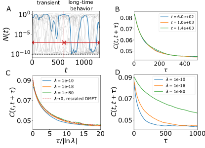
Figure 2: Species dynamics and correlations. (A) Species are initialized with order-one values. We follow $\ln N_{i}(t)$. In the transient regime, the changes in $\ln N_{i}(t)$ are comprised of three elements: downward motion, roughly in straight line (maintaining its slope for a large part of the decay between largest and smallest values, corresponding to exponential decay of $N_{i}$); upward motion, roughly in a straight line; and slow changes at high population values, $N_{i}(t)\simeq O(1)$. The dynamics slow down, with the time spent in each of these elements increasing with the time since the start of the dynamics, see Sec. VI. As the excursions grow longer, the average value of $\ln N_{i}(t)$ decreases linearly in $t$. This transient regime ends when a finite fraction of species reach the migration floor $N_{i}(t)\simeq O(\lambda)$, after a time of order $\left|\ln\lambda\right|$. At long times, after the transient regime is over, $\ln N_{i}(t)$ performs the three dynamical elements described above, and a forth one, slowly changing around the migration floor. The vertical red dashed line marks the crossover between these two regimes. (B) At long times, timescales do not grow in time anymore, as seen in the correlation function that depends only on time differences, $C(t,t^{\prime})=C(t-t^{\prime})$. (C, D) This timescale is proportional to $\left|\ln\lambda\right|$. This is demonstrated by the data collapse when plotting $C$ against $t/\left|\ln\lambda\right|$ presented in panel(C), compared with the data without rescaling shown in (D).

We now describe the long-time phenomenology of the dynamics, when $\lambda>0$. The transient regime, see Fig. 2(A), is later discussed in Sec. VI together with the closely related dynamics of isolated systems, for which $\lambda=0$. When $\lambda>0$ and at long times, the species abundances fluctuate forever and their autocorrelation function $C(t,t^{\prime})\equiv\sum_{i}N_{i}(t)N_{i}(t^{\prime})/S$ becomes time-translation invariant, namely $C(t,t^{\prime})=C(t-t^{\prime})$, see Fig. 2(B). Crucially, the dynamics become slow when $\lambda\ll 1$ and feature an emergent statistical invariance between realizations at different $\lambda$ under the rescaling of time $t\to t/|\ln\lambda|$. As we show in Fig. 2(C), the autocorrelation functions for different values of $\lambda$, but identical values of $\sigma$ and $\mu$, indeed collapse to a single master curve when plotted against $t/\left|\ln\lambda\right|$, namely $C_{\lambda}(t,t+|\ln\lambda|s)\to\hat{C}(s)$ when $\lambda\to 0^{+}$. Thus, a unique timescale $\tau\sim|\ln\lambda|$ characterizes the autocorrelation function. We defer the proof of this result to Sec. IV where we derive the rescaled dynamics, that are also solved numerically to obtain the function $\hat{C}(s)$, see Eqs. (5,7,8).

Timescales of order $|\ln\lambda|$ are expected to appear, since it takes a time $t\sim|\ln\lambda|$ for a population to grow from the migration floor $\lambda$ to $O(1)$ population size under exponential growth with finite growth rate. Importantly, we find that there is no shorter timescale $\tau\ll|\ln\lambda|$ relevant for describing the effective dynamics of a single species. Indeed, the master curve $\hat{C}(s)$ is regular at $s\to 0^{+}$. Recall that $\lambda$ is non-dimensional, and that $|\ln\lambda|$ can be quite large in ecologically relevant contexts, see Section II, in which case fluctuations become correlated over many generation times.

IV Rescaled dynamics

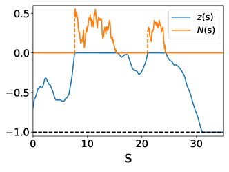
Figure 3: The rescaled dynamics. Trajectories of $N$ and $z\equiv\ln(N)/\left|\ln\lambda\right|$, as a function of the rescaled time $s\equiv t/\left|\ln\lambda\right|$, in an example run of the limiting rescaled dynamics when $\lambda\to 0^{+}$.

In Sec. III we described the phenomenology of the long-time fluctuating dynamics when $0<\lambda\ll 1$. We have seen that the species abundances $N_{i}(t)$ fluctuate over a long timescale of order $|\ln\lambda|$. Furthermore, the log-abundances $\ln N_{i}$ dynamically explore values from $O(\ln\lambda)$ to $O(1)$. These observations motivate defining rescaled variables $s\equiv t/|\ln\lambda|$ and $z_{i}\equiv\ln\left(N_{i}\right)/\left|\ln\lambda\right|$. $z_{i}(s)$ turns out to follow a well-defined stochastic process when $\lambda\to 0^{+}$ (that no longer includes any $\lambda$ dependence). It is a single-variable process describing the probability of trajectories of a single species within the large system. Subsection IV.1 is devoted to the mathematical derivation of this process. Subsection IV.2 describes its properties, and can be read independently of subsection IV.1. Later sections discuss its implications to the species abundance distribution and species diversity.

IV.1 Derivation

Our starting point is the effective single-species stochastic dynamics for $N_{i}(t)$, previously obtained in the limit where the number of species is very large and for any value of $\lambda$ [16]. For the sake of completeness, we briefly outline the steps leading to these dynamics. In Eq. (1), the dynamics of $N_{i}(t)$ are driven by the influence of all other species through $g_{i}(t)=1-\sum_{j}\alpha_{ij}N_{j}(t)$, which involves the sum of many weakly-correlated contributions. Dynamical Mean-Field Theory (DMFT), valid when $S\to\infty$, shows that the $g_{i}(t)$ are identically distributed Gaussian processes, and are independent for $i\neq j$. This implies that population sizes $N_{i}(t)$ behave as independent realizations of the single-variable stochastic process,

$$\dot{N}(t)=N(t)(g(t)-N(t))+\lambda\,.$$ (2)

where the subscript $i$ has been dropped. The first two moments of the Gaussian process $g(t)$ obey self-consistent closure relations, that relate the input noise $g(t)$ to the output $N(t)$,

$$\left\langle g(t)\right\rangle =1-\mu\langle N(t)\rangle\,,$$ (3)

$$\langle g(t)g(t^{\prime})\rangle-\langle g(t^{\prime})\rangle\langle g(t)\rangle =\sigma^{2}\langle N(t)N(t^{\prime})\rangle\,.$$ (4)

Here the angular brackets $\langle.\rangle$ denote an average over the realizations of $g(t)$ (and the initial conditions $N(0)$ which are irrelevant at large times). The derivation of Eq. (2) follows a standard procedure [36, 37, 38, 39] which was applied to the Lotka-Volterra equations in [16]. In the long-time limit where $\langle N(t)\rangle\to\langle N\rangle,$ the entire dynamics is controlled by the two-time correlation $C(t,t^{\prime})\equiv\langle N(t)N(t^{\prime})\rangle$, since the Gaussian process $g(t)$ is completely characterized by its correlations and mean, given in (3,4).

In order to study the behavior of these equations when $\lambda\ll 1$, we introduce $z\equiv\ln(N)/|\ln\lambda|$ and $s\equiv t/|\ln\lambda|$ so that Eq. (2) becomes

$$z^{\prime}(s)=g(s)+\exp(-|\ln\lambda|(z(s)+1))-\exp(|\ln\lambda|z(s))\,.$$

The non-linear terms become impenetrable boundaries when $\lambda\to 0^{+}$, since

$$\lim_{\lambda\to 0^{+}}\exp(-|\ln\lambda|(z+1))=\begin{cases}0&\text{if $z>-1\,,$}\\ +\infty&\text{if $z<-1$\,,}\end{cases}$$

and

$$\lim_{\lambda\to 0^{+}}\exp(|\ln\lambda|z)=\begin{cases}0&\text{if $z<0\,,$}\\ +\infty&\text{if $z>0$\,.}\end{cases}$$

Hence the process $z(s)$ is confined between $-1$ and $0$ when $\lambda\to 0^{+}$. The confinement originates from the migration term and the self-regulation term, proportional to $N_{i}^{2}$, in Eq. (1). The effective noise $g(s)$ is not able to push $z(s)$ to outside of the confining region, because its mean and variance are finite provided population sizes do not blow up, see Eqs. (3,4). Thus $z(s)$ obeys

$$z^{\prime}(s)=g(s)+W(z+1)-W(z)\,,$$ (5)

in the low migration limit, where $W(z)$ and $W(z+1)$ account for the confining boundaries at $z=0$ and $z=-1$. The autocorrelation function of $g(s)$ is proportional to the master function $\hat{C}(s)$ introduced in Sec. III, since $\langle g(s)g(s^{\prime})\rangle-\langle g(s^{\prime})\rangle\langle g(s)\rangle=\sigma^{2}\langle N(s)N(s^{\prime})\rangle=\sigma^{2}\hat{C}(s-s^{\prime})$.

We now derive the evolution of the abundance $N(s)$. Beyond the fact that $N(s)$ is the main quantity of interest, such an evolution is also necessary to derive the self-consistent equations (3,4) in the the $\lambda\to 0^{+}$ limit, and obtain a closure of the DMFT equations in terms of the process $z(s)$. When $z(s)<0$ it is clear from the definition $N(s)=\exp\left(\left|\ln\lambda\right|z(s)\right)$ that $N(s)=0$ in that limit. However, this relation appears ambiguous in the double limit $z\to 0$ and $\lambda\to 0^{+}$. To remove the ambiguity we use the impenetrability condition at the $z=0$ boundary, namely $W(z(s))=g(s)$ when $z(s)=0$. Since by definition of $z$ and Eq. (5), $W(z(s))=N(s)$, we obtain the relation

$$N(s)=g(s)\Theta(z(s))\,,$$ (6)

where $\Theta(z)$ is the Heaviside function with the convention $\Theta(0)=1$. The existence of this impenetrability condition rests on the facts that (i) $g(s)$ does not have a white noise component, which follows from the fact that its mean and variance remain finite when $\lambda\to 0^{\text{+}}$ and (ii) that $\hat{C}(s)$ has a well-defined limit when $\lambda\to 0^{+}$, which agrees with numerical simulations (see Fig. 2(C)). That $\hat{C}(s)$ is well-behaved when $\lambda\to 0^{+}$ is for now assumed and is self-consistently verified is the following Eqs. (7,8). The interpretation of Eq. (6) is discussed below in Sec. IV.2.

Using Eq. (6), the $\lambda\to 0^{+}$ limit of the closure equations (3,4) reads

$$\langle g(s)\rangle =1-\mu\langle g(s)\Theta(z(s))\rangle\,,$$ (7)

$$\langle g(s)g(s^{\prime})\rangle-\langle g(s^{\prime})\rangle\langle g(s)\rangle =\sigma\langle g(s)g(s^{\prime})\Theta(z(s))\Theta(z(s^{\prime}))\rangle\,.$$ (8)

Importantly, Eqs. (5,7,8) are independent of $\lambda$. It therefore follows that indeed, $g(s)$ has well-defined correlations in the limit $\lambda\to 0^{+}$.

IV.2 Properties of the limit dynamics

Equation (5) describes the effective evolution of $z_{i}(s)$ for any single species within the many-variable system. It is driven by a Gaussian noise $g_{i}(s)$ and confined to values $-1\leq z_{i}\leq 0$. The mean and variance of the Gaussian noise $g_{i}(s)$ are determined self-consistently through Eqs. (3,4), which become Eqs. (7,8) in the limit $\lambda\to 0^{+}$. The noise $g_{i}(s)$ can be interpreted within the original many-species species dynamics Eq. (1) as the effective growth rate set by all the other species, $g_{i}(s)=1-\sum_{j}\alpha_{ij}N_{j}(s)$, which can indeed be shown to be Gaussian distributed in the limit of many species. When $-1<z_{i}(s)<0$, meaning $\lambda\ll N_{i}\ll 1$, the dynamics read $z_{i}^{\prime}(s)=\dot{N_{i}}(t)/N_{i}(t)=g_{i}(s)$, resulting in exponential growth or decay of the population sizes under the effective growth rate set by all the other species.

In the limit $\lambda\to 0^{+}$, the dynamics of the population size $N_{i}(s)$ is related to that of $z_{i}(s)$ by Eq. (6). When $z_{i}(s)<0$, Eq. (6) yields $N_{i}(s)=0$ which naturally follows from taking the limit $\lambda\to 0^{+}$ in the definition $N_{i}=\exp(|\ln\lambda|z_{i})$. Yet Eq. (6) goes further, relating $N_{i}$ and $z_{i}$ in the double limit where both $\lambda\to 0^{+}$ and $z_{i}=0$. The interpretation of Eq. (6) is that the species with $z_{i}=0$, meaning with a finite population size $N_{i}$, are in a slowly-changing fixed point. Indeed, Eq. (6) can also be obtained from the many-body dynamics using the slowness of the dynamics discussed in Sec. III when $\lambda\to 0^{+}$: by Eq. (1), slow changes $\dot{N}_{i}(t)\simeq 0$ require $N_{i}(t)=g_{i}(t)$ when $N_{i}(t)$ is finite.

Equations (3,4) guarantee that $g(s)$ has finite variance and mean, so that $g(s)$ can not contain a white noise component. Also, by solving these rescaled DMFT equations following the procedure detailed in Appendix 13, we find that $\hat{C}^{\prime}(0^{+})$ is finite, thus confirming the absence of fast-time scale in the Lotka-Volterra dynamics, see Fig. 8. We further show that $\hat{C}^{\prime}(0^{+})\neq 0$, meaning that $g(s)$ is rough, namely nowhere differentiable (like in Brownian motion ). The fact that $\hat{C}^{\prime}(0^{+})\neq 0$ follows from Eq. (10) below, see the discussion there. An example run of the rescaled dynamics is shown in Fig. 3. As can be seen, $-1\leq z\leq 0$, and $z$ spends finite time intervals at the boundaries, which is a consequence of the finite memory of the noise $g(s)$. Indeed, if $g>0$ and $z=0$ at a given time, it will remain so for a finite amount of time.

Lastly, we discuss important features of the dynamics of the population sizes $N(s)$ seen in Fig. 3. First, $N(s)$ is rough since $N=g$ when $z=0$, while $z(s)$ is more smooth since it is an time integral of $g(s)$. Second, the limiting process $N(s)$ is not continuous in time and features jumps from $0$ to a finite value, after which $N(s)$ continuously reaches $0$. The jumps represent species that grow from very small abundances at a finite growth rate, and thus their time to reach $N=g$ from a small fixed value (that doesn’t depend on $\lambda$, say $N=10^{-5}$) is finite in time $t$, and so vanishes in the rescaled time $s$. These jumps are precisely species turnover events, that drive the change in the composition of the abundant species.

V Phenomenology revisited

V.1 Diversities revisited

In Sec. III.1, we proposed three definitions for diversity $S_{\text{top}}^{*},S_{\text{inter}}^{*},S_{\text{growth}}^{*}$. Denote $\phi_{\text{top}}\equiv S_{\text{top}}^{*}/S$ and similarly for $\phi_{\text{inter}},\phi_{\text{growth}}$. All these quantities are well-defined in the limit $\lambda\to 0^{+}$. Indeed, they take simple forms in terms of the limiting process described in Sec. IV:

$$\phi_{\text{top}} =\text{Prob}[z=0]\,,$$

$$\phi_{\text{inter}} =1-\text{Prob}[z=-1]\,,$$

$$\phi_{\text{growth}} =\text{Prob}[g>0]\,.$$ (9)

We now return to the discussion of $\phi_{\text{top}}$ and its relation to the stability bound, see Sec. III.1. As followed from the rescaled dynamics, the abundant species counted in $\phi_{\text{top}}$ are approximately at a fixed point, while all other species have negligible abundances, and so do not affect this fixed point. Thus, one indeed expects the bound $S_{\text{top}}^{*}\text{var}(\alpha)=\sigma^{2}\phi_{\text{top}}\leq 1$ to hold, as is clear in Fig. 1(G). Indeed, a fixed point with $S_{\text{top}}^{*}$ coexisting species and $S_{\text{top}}^{*}\text{var}(\alpha)>1$ would be typically linearly unstable to perturbations [11, 12, 35].

A natural question is: Is the stability bound saturated, i.e. $\sigma^{2}\phi_{\text{top}}=1$, resulting in fixed points of abundant species that are near marginal stability? One could perhaps expect marginal stability, as the rate at which low-abundance species are added to the subset of abundant ones is slow, “gently” perturbing the fixed points, and so would perhaps allow $S_{\text{top}}^{*}$ to increase up to the stability bound. In addition, marginality is reached in Lotka-Volterra dynamics [35], Eq. (1), with symmetric interactions ($\alpha_{ij}=\alpha_{ji}$). And more generally, slow dynamics are in many cases associated with marginality (see, e.g., [41]).

Yet, as was shown in Sec. III.1, see Fig. 1(G), $\sigma^{2}\phi_{\text{top}}<1$ so the stability bound is not saturated. Consequently, as $\lambda\to 0^{+}$, the high-abundance species lie at any time in the vicinity of a fixed point that is linearly stable to perturbations applied to those species. Note that this fixed point changes over time, as it is destabilized by the growth of species from rare.

To obtain the bound $\sigma^{2}\phi_{\text{top}}<1$, we prove that while species turnover is a slow process, the jumps when going from rare to abundant, seen clearly in Fig. 3, are sufficient to significantly perturb the subset of abundant species and prevent it from reaching marginal stability. We prove that by deriving an exact relation that links diversity with temporal fluctuations, defined as follows. Let $N_{\text{jump}}$ be the size of these jumps. Let $G$ be the rate of incoming species weighted by $N_{\text{jump}}^{2}$: that is, the sum of $N_{\text{jump}}^{2}$ over all jumps taking place in a unit of rescaled time $s$ in the many-species dynamics, and divided by the number of species $S$. The relation, derived in Appendix A.3, reads:

$$G=2\left|\hat{C}^{\prime}\left(0^{+}\right)\right|\left(1-\sigma^{2}\phi_{{\rm top}}\right)\ .$$ (10)

Here $\hat{C}\left(s\right)$ is the autocorrelation of $N(s)$ in the rescaled time defined in Sec. III. $\hat{C}^{\prime}\left(0^{+}\right)$ is finite, see Fig. 2(C) and Fig. 8 in Appendix A.1. Eq. (10) then limits $\phi_{\text{top}}$ to be below the stability bound; indeed, marginal stability $1=\sigma^{2}\phi_{{\rm top}}$ is only possible if $G=0$, namely species do not perform jumps, in contradiction with the dynamics in Sec. IV. Additionally, we note that $G>0$ implies $\left|\hat{C}^{\prime}\left(0^{+}\right)\right|>0$, thus proving that the trajectories $N_{i}(s)$ are rough when $N_{i}(s)\neq 0$.

Put differently, the introduction of one new species leads to the removal of others, with the average number of removed species growing as one approaches the marginal diversity. The balance, in which one species is removed for each one introduced, sets $S_{\text{top}}^{*}$, that only reaches some fraction of the bound $1/\mathrm{var}(\alpha)$. In dynamics that reach a fixed point, the requirement that all species involved have positive abundance is known as feasibility [42], and it is what limits the diversity in the fixed point phase, $\sigma<\sigma_{c}$ in Fig. 2(F). Eq. 10 can be thought of as an extension of the requirement to dynamics, a form of “dynamical feasibility”.

V.2 Species Abundance Distribution revisited

We now return to the species abundance distribution $P(N)$. As mentioned in Sec. III.1, $P(N)$ behaves roughly as $1/N$ in the intermediate range $\lambda\ll N\ll 1$. Using the rescaled dynamics, we can refine this statement. The dynamics of $z_{i}(s)$ (Sec. IV) spend a finite fraction of the time at the boundaries $z=-1,0$. This translates to two delta-peak contributions in $P(z)$ at these values. In addition, there is a regular contribution for $-1<z<0$. Together, this reads

$$P(z) = \phi_{\text{top}}\,\delta(z)+\left(1-\phi_{\text{inter}}\right)\delta(z+1)$$ (11)

$$+(\phi_{\text{inter}}-\phi_{\text{top}})h(z)\Theta(-z)\Theta(1+z)\,,$$

where $h(z)$ is a smooth function with $\int_{-1}^{0}h(z)\,dz=1$. $\phi_{\text{top}},\phi_{\text{inter}}$ were defined in Eq. (9). Fig. 4(B) shows the collapse of $P(z=\ln N/|\ln\lambda|)$ as $\lambda\to 0^{+}$ to this form.

Eq. (11) sets the form of the abundance distribution in the intermediate range $\lambda\ll N\ll 1$. Changing variables from $z$ to $N$, we get

$$P(N)=\frac{1}{N\left|\ln\lambda\right|}\>h\negthinspace\left(\frac{\ln N}{\left|\ln\lambda\right|}\right)\ .$$ (12)

This refines the $1/N$ dependence with an additional, slowly-varying correction. As we discuss in Sec. VIII, this correction can appear to change the power law exponent of the species abundance distribution when $\lambda$ is finite, and only parts of the entire distribution are sampled. The distribution of top species can be inferred from $P[g|z]$, the distribution of the growth rate $g$ conditioned on the value of the rescaled abundance $z$. For $N\geq 0$, we get

$$P(N)=\phi_{\text{top}}P\left[g=N|z=0\right]+(1-\phi_{\text{top}})\delta(N)\,.$$ (13)

Fig. 4(A) shows the convergence of the distribution $P(N)$ to this limiting distribution as $\lambda\to 0^{+}$. The results in the limit $\lambda\to 0^{+}$ were obtained by solving numerically the rescaled DMFT equations, see Eqs. (5,7,8). The limiting distribution $P(N)$ deviates from the truncated Gaussian SAD obtained in the fixed point phase.

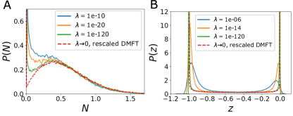
Figure 4: Collapse of species abundance distributions. Numerically measured distributions of $N$ (A) and $z=\ln N/|\ln\lambda|$ (B) converge to the distributions predicted by the rescaled process as $\lambda\to 0^{+}$.

VI Dynamics of an isolated system and transient dynamics at finite $\lambda$

VI.1 Dynamics of an isolated system

Isolated systems are characterized by zero migration rate, $\lambda=0$, which is a singular limit of the Lotka-Volterra system of equations with a large number of species, in the chaotic phase. Indeed, the timescale $|\ln\lambda|$ which characterizes these dynamics at finite $\lambda$, diverges when $\lambda\to 0$. For $\lambda=0$, the dynamics are not time-translation invariant but forever slow down in time, as evidenced in a linear growth of the correlation time as a function of the elapsed time, a behavior known in physics as ‘aging’. Formally, $C_{\lambda=0}(t,t+tt^{\prime})\to\hat{C}(t^{\prime})$ when $t$ is large, see Fig. 5(A) for the collapse of results from numerical simulations. Again, the master curve $\hat{C}(t^{\prime})$, which depends on the parameters $\sigma$ and $\mu$, is regular at $t^{\prime}\to 0^{+}$. This behavior can be understood as follows: When $\lambda=0$ the lowest values of $\ln N$ reached after time $t$ are of order $\ln N\sim-t$. If a species changes to positive growth rate at this time, it will therefore take another time $t$ for its population size to be $O(1)$. This sets the correlation time. A similar mechanism was found in another, exactly-solvable, model [21].

The proof of the existence of this aging regime is given in App. A.2. Using a reasoning similar to that employed in Sec. IV, we show that the transformed variables $s\equiv\ln t,z\equiv\ln(N)/t$ obey a well-defined set of DMFT equations which become time-translation invariant when $t\to\infty$. These transformations reflect a growth of both timescales and log-fluctuations with the elapsed time. The resulting process $z(s)$ is different from that of Sec. IV, and is described in detail in Appendix A.2.

An important consequence of this result is that the collective deterministic dynamics in an isolated system drives the population size of any species arbitrarily close to $0$ as time grows. Considering that actual populations sizes are finite, integer numbers, this process will inevitably lead to the extinction of many species, subsequently leading to an arrest of the fluctuations, as suggested in [17, 18].

VI.2 Transient dynamics at finite $\lambda$

When migration is present, this dynamical slowdown provides a mechanism by which the correlation time grows until time $t_{\textrm{transient}}\sim|\ln\lambda|$, where the correlation time reaches the value $|\ln\lambda|$ discussed above. This is indeed the time it takes for a finite fraction of the species in the community to reach the migration floor, when starting with all species with population sizes of $O(1)$, and before which $\lambda$ can be safely set to zero.

We verify in simulations that the transient dynamics is characterized by a linear growth of timescale with the elapsed time, which is interrupted at a time $t_{\textrm{transient}}\sim|\ln\lambda|$. For that, we measure the time constant $\tau_{2}(\lambda,t)$ it takes for the autocorrelation function $C_{\lambda}(t+\tau,t)-C_{\lambda}(\infty,t)$ to reach a fraction $e^{-1}$ of its $\tau=0$ value, starting at initial time $t$ and with migration rate $\lambda$. Fig. 5(C) shows that the growth and saturation of the timescale follow the scaling relation

$$\frac{\tau_{2}(\lambda,t)}{|\ln\lambda|}=f\left(\frac{t}{|\ln\lambda|}\right)\,,$$

where $f$ is a smooth function with $f(x)\propto x$ at small $x$, encoding the slowdown of the dynamics in the transient regime, and $f(x)$ approaching a constant as $x\to\infty$, encoding the time-translation invariant behavior of the long-time dynamics, with correlation timescale $|\ln\lambda|$.

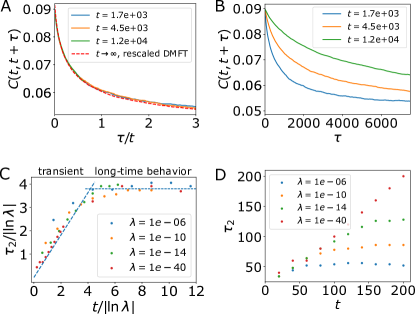
Figure 5: Growth of timescales in dynamics without migration. (A,B) When $\lambda=0$, the collapse of $C(t,t+\tau)$ as a function of $\tau/t$ demonstrates the linear growth of timescales with the elapsed time. Data without rescaling, as a function only of $\tau$, is shown for comparison in (B). (C,D) Crossover at finite $\lambda$ from a transient regime exhibiting the $\lambda=0$ phenomenology to the long-time behavior, as identified by the time constant $\tau_{2}$ of the correlation function. After an initial transient of finite time duration, $\tau_{2}$ grows linearly with the elapsed time and independently of $\lambda$, a trademark of the $\lambda=0$ dynamics. The crossover to the long-time behavior happens around times proportional to $|\ln\lambda|$, after which $\tau_{2}$ stabilizes to a value proportional to $\left|\ln\lambda\right|$. This scaling of the crossover is manifest in the data collapse in (C), with the data without rescaling displayed in (D) for comparison. $\tau_{2}(t,\lambda)$ is defined as the time when $\left[C(t,t+\tau_{2})-C(t,\infty)\right]/\left[C(t,t)-C(t,\infty)\right]=e^{-1}$. The value of $C(t,\infty)$ is estimated through an exponential fit of the function $C(t,t+\tau)$ as a function of $\tau$.

VII Robustness of the predictions

The theory is built around two limits, $S\to\infty$ and $\lambda\to 0^{+}$, and assumes that the interaction coefficients $\alpha_{ij}$ are sampled independently. In this last part of this work, we assess the robustness of our predictions when these assumptions are relaxed. We find that the main qualitative features discussed in this work are robust against changes in model definition, and relevant even at reasonable values of migration rate and number of species.

VII.1 Finite migration rate $\lambda$ and number of species $S$

We start by discussing how the key quantities, $\left\langle N\right\rangle$, $\left\langle N^{2}\right\rangle$ and $\phi_{{\rm top}}$ vary with $S,\lambda$, when measured from abundance data gathered in numerical simulations of the original many-species dynamics Eq. (1). Regarding the moments $\left\langle N\right\rangle,\left\langle N^{2}\right\rangle$, we find that the dependence on $S$ and $\lambda$ is very weak for $\left\langle N\right\rangle$ and weak for $\left\langle N^{2}\right\rangle$, respectively within roughly 1% and 10% in the inspected range of parameter, see Fig. 11 in Appendix A.5.

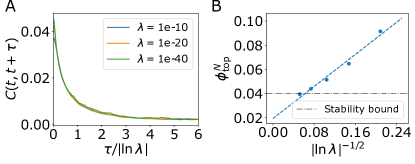
Figure 12: Model behavior at higher values of $\sigma,\mu$. (A) Collapse of the correlation function $C_{\lambda}(t,t+\tau)$ as a function of $\tau/\left|\ln\lambda\right|$, showing that the only timescale in the problem scales as $\left|\ln\lambda\right|$. Compare with Fig. 2(C). (B) $\phi_{{\rm top}}^{\text{N}}$ as a function of $\lambda$, showing the same dependence on $\lambda$, converging as $\left|\ln\lambda\right|^{-1/2}$. Compare with Fig. 6(B). The extrapolated asymptotic value at $\lambda\to 0^{+}$ is well-below the May bound. Here, $\sigma=5$, $\mu=50$, $S=5000$. $\phi_{{\rm top}}^{\text{N}}$ is defined with $N_{i}>\epsilon=10^{-3}$.

To measure $\phi_{{\rm top}}$ at finite $\lambda$, we test three options. The first measure, $\phi_{{\rm top}}^{\text{N}}(S,\lambda,\epsilon)$, is simply a threshold on the abundance: counting all the species with $N_{i}\geq\epsilon$ at a given time, for some chosen $\epsilon$. Unsurprisingly, $\phi_{{\rm top}}^{\text{N}}(S,\lambda,\epsilon)$ is more sensitive to $\lambda$ than $\left\langle N\right\rangle$ or $\left\langle N^{2}\right\rangle$. For moderate values of $S$ and $\lambda$, we find that the asymptotic value $\phi_{{\rm top}}$ nevertheless provides a reasonable estimate of $\phi_{{\rm top}}^{\text{N}}(S,\lambda,\epsilon)$, see Fig. 6(A, B), though the discrepancy increases with the strength of the interactions, see Fig. 12(B). This last point suggests that disentangling species at high and intermediate abundances becomes harder when the scale of the interactions, and thus the amplitude of the fluctuations, increases. The second measure, denoted by $\phi_{{\rm top}}^{\text{g}}(S,\lambda,\epsilon)$, refines the first one and requires $N_{i}\geq\epsilon$ but also $g_{i}>0$. We find that both measures converge to the asymptotic $\phi_{{\rm top}}$ as $1/S$ in $S$. Yet the convergence with $\lambda$ is significantly different, with $\phi_{{\rm top}}^{\text{N}}$ converging as $\left|\ln\lambda\right|^{-1/2}$, and $\phi_{{\rm top}}^{\text{g}}$ faster, as $\left|\ln\lambda\right|^{-1}$, see Fig. 6(B, D). This highlights the relevance of the growth rate $g$ in determining “top species”, namely members of fixed points. We find that the measure $\phi_{{\rm top}}^{\text{N}}(S,\lambda,\epsilon)$ is often above the stability bound, in contrast to the asymptotic $\phi_{{\rm top}}$ which is always below it. Due to the faster convergence, $\phi_{{\rm top}}^{\text{g}}(S,\lambda,\epsilon)$ can be either above or below this bound, depending on the parameters, see Fig. 6(C). The origin of these convergence rates is discussed in Appendix A.4.

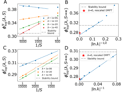
Figure 6: Average top diversity measures, $\phi_{{\rm top}}^{\text{N}}(S,\lambda,\epsilon),\phi_{{\rm top}}^{\text{g}}(S,\lambda,\epsilon)$, as a function of $S$ and $\lambda$. $\phi_{{\rm top}}^{\text{N}}$ is the fraction of species with $N_{i}>\epsilon=10^{-3}$; $\phi_{{\rm top}}^{\text{g}}$ also requires $g_{i}>0$. (A) $\phi_{{\rm top}}^{N}(S,\lambda,\epsilon)$ as a function of $S$ converges as $\phi_{{\rm top}}^{N}(S\to\infty,\lambda,\epsilon)+\#/S$, at fixed $\lambda$. Data points at $S=500$ are excluded from the linear fit. (B) Large $S$ value of the top diversity, $\phi_{{\rm top}}^{N}(S\to\infty,\lambda,\epsilon)$, converges as $\left|\ln\lambda\right|^{-1/2}$ to its asymptotic value $\phi_{{\rm top}}^{N}(S\to\infty,\lambda\to 0^{+},\epsilon)$. The asymptotic value $\phi_{{\rm top}}^{N}(S\to\infty,\lambda\to 0^{+},\epsilon)$ is within 5% of the value predicted by the rescaled DMFT, and well below the stability bound. For all reasonable values of the migration rate, (here already when $\lambda\gtrsim 10^{-40}$), the measured top diversity is significantly above the stability bound. $\phi_{{\rm top}}^{N}(S\to\infty,\lambda,\epsilon)$ was inferred from the finite $S$ scaling, panel A. (C,D) Same as panels A,B, but for $\phi_{{\rm top}}^{\text{g}}(S,\lambda,\epsilon)$. The convergence to the asymptotic $\phi_{{\rm top}}$ is more rapid; in particular, $\phi_{{\rm top}}^{\text{g}}$ can be either below or above the stability bound.

Finally, we consider a situation where one is able to manipulate the system, by removing certain species and continuing the dynamics. Namely, after a long time so that transients have passed, we kill all species with $N_{i}/g_{i}<1/2$. These correspond to species with positive growth rate that are in the midst of their jump, below halfway, as well as those with negative growth rate. (Recall that, asymptotically as $\lambda\to 0^{+}$, abundant species are those for which that $N_{i}/g_{i}=1$.) Then, we run again the dynamics, and we find that the remaining species reach a stable equilibrium. The properties of the equilibrium obtained in this way are strikingly similar to those predicted by the asymptotic theory, even for reasonable $\lambda$. The asymptotic diversity and the asymptotic distribution in Eq. (13) can be almost exactly reproduced, see Appendix A.6.

VII.2 Correlation between the matrix elements

In addition to taking the asymptotic limits in $S,\lambda$, the model above assumes that interactions are statistically asymmetric with vanishing correlation coefficient $\text{corr}(\alpha_{ij},\alpha_{ji})=0$. We show that two of our main qualitative results–how the timescale grows and that top diversity is below the stability bound–also hold when this assumption is relaxed. Allowing for more symmetric or anti-symmetric interactions, we take a correlation coefficient $\text{corr}(\alpha_{ij},\alpha_{ji})=\gamma$ with $-1<\gamma<1$.

The growth of the timescale $\tau\sim\tau_{\lambda}\equiv\left|\ln\lambda\right|$ is clearly seen in Fig. 10(A,B) in Appendix A.4, the equivalent of Fig. 2(C). This is expected for the same reason as when $\gamma=0$: the time for a population to grow from $\lambda$ to $N\sim 1$ scales as $\left|\ln\lambda\right|$. As to the diversity $\phi_{\text{top}}$, we conjecture that the slowness of the dynamics at $\lambda\ll 1$ still introduces a clear partition between nearly-extinct species with $\ln N\sim\ln\lambda$ and abundant species with $N=O(1)$. For the abundant species, the long timescale implies that they are near a fixed point. In Appendix A.4, we generalize the relation between fluctuations and diversity from Sec. V.1, Eq. (10), to give

$$G=2|\hat{C}^{\prime}\left(0^{+}\right)|\ \frac{\left(1+\sqrt{1-4\gamma\phi_{{\rm top}}\sigma^{2}}\right)^{2}-4\phi_{{\rm top}}\sigma^{2}}{\left(1+\sqrt{1-4\gamma\phi_{{\rm top}}\sigma^{2}}\right)^{2}}\,.$$ (14)

As for $\gamma=0$, we expect that the growth of timescale when $\lambda\to 0^{+}$ goes hand-in-hand with jumps in the rescaled dynamics of the abundances, meaning $G>0$. This implies $\left(1+\sqrt{1-4\gamma\phi_{{\rm top}}\sigma^{2}}\right)^{2}-4\phi_{{\rm top}}\sigma^{2}>0$, so that $\phi_{{\rm top}}$ lies strictly below the linear stability bound [13]. This is confirmed by numerical simulations, see Fig. 10(C,D) in Appendix A.4.

VIII Discussion

We begin the discussion by summarizing key predictions presented above. We identified several signatures of the many-species Lotka-Volterra dynamics, when the abundnaces does not reach a fixed point and migration rates are small. They may serve as footprints of endogenously-driven fluctuations in experimental or natural situations.

First, we predict that endogenously-driven fluctuations in time would lead to broadly distributed abundance distributions, in contrast with the fixed point distributions. For very low migration, the abundance distribution at intermediate values (meaning small population sizes well above the migration floor) are predicted to behave as $P(N)\sim 1/N$. At any finite $\lambda$, there are slowly varying corrections to this $1/N$ behavior, see Eq. (12). As $P(N)$ is broad, one can always define a slowly-varying ‘local’ power law $\nu(z)$ by the slope of $\ln P(N)$ versus $\ln N$ at given $z=\ln N/\left|\ln\lambda\right|$. It has corrections of order $|\ln\lambda|^{-1}$, $\nu(z)=-1+|\ln\lambda|^{-1}h^{\prime}(z)/h(z)$, which might explain deviations from $\nu=-1$ in observed abundance distributions [6]. These corrections vary with $z$ and are arbitrarily large over the entire range $-1<z<0$, so no unique exponent other than $-1$ can be defined over the entire range of $N$.

Second, we predict that a single timescale controls the dynamics, predicted to grow as $|\ln\lambda|$ when lowering the migration rate. This could be tested in controlled experiments, for example via the abundance autocorrelation.

Moving on to diversity, different definitions of diversity give different results. For example, the number of species that can grow from rare at a given time, is generally different from the number of species that have high abundance, in contrast with the situation at a fixed point. We show that the number of species with high, intermediate and low abundance is well defined, namely insensitive to the precise threshold above (or below) which the number of species is counted. We show that the number of species at high abundance is significantly below the May bound (their fraction of the total number of species is below the fraction allowed by the bound). This makes the community of high-abundance species a stable equilibrium of the dynamics if the other species are removed. The distance to the stability bound increases with the strength of the interactions $\sigma$, see Fig. 1(G), and also Fig. 12(B) in Appendix A.4. In contrast, when including the intermediate ones (in the power law regime of $P(N)$), the total number goes above the bound. The same is true when including all species in the pool that may invade. It is this last fact that drives species turnover: there are always species that grow from rare to replace the ones at high abundance.

Last, a key property of the dynamics at low migration is the existence of jumps from rare in the dynamics of population sizes, see Fig. 3. For finite $\lambda$, this manifests itself in a strong asymmetry of “blooms”, namely trajectories where the abundance of a species increases from rare before returning there. This can be clearly observed in time series at finite $\lambda$, see Fig. 7, and would be very interesting to look for in experimentally-measured time series.

In conclusion, the dynamically-fluctuating phase of high-diversity ecological communities is a promising direction to explain key features of natural high-diversity ecosystems. We offered a list of additional predictions expected in this phase. It would be interesting to further investigate the robustness of these features upon modifying the structure of the interaction matrix. Along this line, we note that the chaotic dynamics appear at finite $S$ also without any beneficial interactions ($\alpha_{ij}<0$) between species, and the analysis above is expected to hold. We further note that the limit of large $\sigma,\mu$ in our framework connects to other asymptotic limits [18, 43]. A recent work on the strongly interacting case [44] suggests from numerics that the qualitative picture of the present study may extend to that regime, in particular the existence of a growing timescale, and the fact that dynamics evolve in the vicinity of fixed points. A different and very interesting direction for future research is understanding how these results extent to spatially-extended metacommunities [17, 18], beyond a constant migration from an unspecified species pool, as assumed here. This question is pertinent, given that the present work shows that chaotic fluctuations cannot generically be sustained in isolated high-diversity systems, due to extinctions.

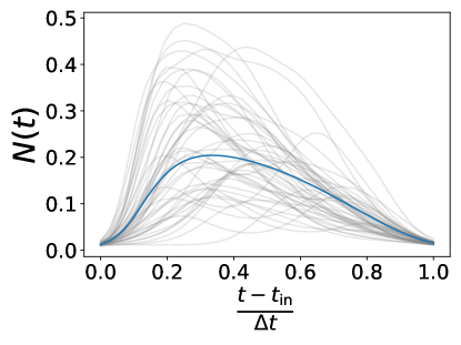
Figure 7: Asymmetry of blooms under time-reversal. Trajectories of $N(t)$ while at high-abundance display a clear asymmetry in time, with a rapid initial increase and more gradual decrease. This is conspicuous even for migration rates that are not very small (here $\lambda=10^{-6}$). It is the finite-$\lambda$ counterpart of the asymptotic behavior at $\lambda\to 0^{+}$, featuring sharp jumps from zero to positive $N$, see Fig. 3. Shown are trajectories that go above $N=10^{-2}$ at some time $t_{\text{in}}$ and stay above it until time $t_{\text{in}}+\Delta t$, and reach $N\geq 0.1$ at some intermediate time. Here $\Delta t\simeq 5.8\left|\ln\lambda\right|$ that is the most common length of such trajectories. In light grey are 22 example trajectories, and the thick blue line shows the average over many such trajectories.

Acknowledgments–This work was supported by the Israel Science Foundation (ISF) Grant No. 773/18.

Appendix A Derivations

A.1 Regularity of the correlation function as $\lambda\to 0^{+}$

By solving the DMFT equations Eqs. (5,7,8) following the procedure detailed in App. (13), we find that $\hat{C}^{\prime}(0^{+})$ is finite, thus confirming the absence of fast-time scale in the Lotka-Volterra dynamics, see Fig. 8.

Figure 8: Zoom on the small $s$ behavior of $\hat{C}(s)$. The correlation function was obtained by numerically solving the DMFT equations Eqs. (5,7,8). The derivative is finite at $s=0^{+}$, thereby confirming the absence of fast-time scale in the Lotka-Volterra dynamics.

A.2 Rescaled dynamics for $\lambda=0$

In this section, we adapt the derivation of Sec. IV to the singular case $\lambda=0$ that accounts for the initial transient when $0<\lambda\ll 1$. For $0<\lambda\ll 1$, the system reaches a time-translation invariant state with correlations characterized by a unique time-scale $|\ln\lambda|$. The latter diverges as $\lambda\to 0^{+}$, suggesting that the $\lambda=0$ dynamics does not reach a time-translation invariant state. We show that the dynamics age with a correlation time that grows linearly with the elapsed time, a phenomena already identified in a related population dynamics model [21],

$$\lim_{t\to\infty}C_{\lambda=0}(t,t\text{e}^{s})=\hat{C}(s)\,.$$ (15)

This scaling regime can be shown to be a self-consistent solution of the dynamical mean-field theory equations Eqs. (2,3,4) with $\lambda=0$. We introduce $z\equiv\ln N/t$ and $s\equiv\ln t$ and obtain from Eq. (2)

$$z^{\prime}(s)=-z(s)+g(s)-\exp(e^{s}z(s))\,.$$

Under the assumption that Eq. (15) holds, the Gaussian process $g(s)$ has a time-independent mean and finite memory with time-translation invariant correlations in the large $s$ limit. Similarly to the $\lambda\to 0^{+}$ case, the term $-\exp(e^{s}z)$ effectively acts as a hard wall at $z=0$ thus constraining $z(s)\leq 0$. The long-time dynamics therefore writes

$$z^{\prime}(s)=-z(s)+g(s)-W(z),$$ (16)

with $W(z)$ formally accounting for the presence of the confining boundary. We use the non-penetrability condition to resolve the ambiguous expression $N(s)=\exp(e^{s}z)$ in the double limit $s\to\infty$ and $z\to 0$ and get

$$N(s)\equiv W(z(s))=g(s)\Theta(z(s))\,,$$ (17)

with the convention $\Theta(0)=1$. It shows that Eq. (16) is supplemented by the same self-consistency conditions as in the $\lambda\to 0^{+}$ case, see Eqs. (7,8)

$$\langle g(s)\rangle=1-\mu\langle g(s)\Theta(z(s))\rangle\,,$$ (18)

together with

$$\langle g(s)g(s^{\prime})\rangle-\langle g(s^{\prime})\rangle\langle g(s)\rangle=\sigma^{2}\langle g(s)g(s^{\prime})\Theta(z(s))\Theta(z(s^{\prime}))\rangle\,.$$ (19)

Note however that in the $\lambda=0$ case, the process $z(s)$ is confined in the negative half-line by a harmonic potential and not by a hard boundary, see Eq. (16).

Under the condition that $g(s)$ has time-translation invariant correlations, Eq. (16) manifestly predicts that $z(s)$ reach at long time a time-translation invariant state. The closure equations Eqs. (18)-(19) then self-consistently show the validity of the time-translation invariant ansatz in rescaled time $s$, eventually showing the validity of the aging scaling given in Eq. (15). In Fig. 9, we show the large-time convergence of the distributions $P(N)$ and $P(z)$ to those predicted by the $\lambda=0$ rescaled dynamics presented here.

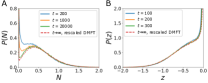
Figure 9: Collapse of species abundance distributions. Numerically measured distributions of $N$ (A) and $z=\ln N/t$ (B) converge to the distributions predicted by the rescaled process as $t\to\infty$.

A.3 Diversity limited by fluctuations

The two cases $\lambda\to 0^{+}$ and $\lambda=0$ share a crucial property: the long-time dynamics are very slow, reflecting the fact that the system evolves in the vicinity of feasible fixed points (all population sizes are $\geq 0$). More precisely, at any given time $s$, the system is close to a fixed point comprised of some abundant species with $O(1)$ population sizes (corresponding to the fraction $\phi_{{\rm top}}$ of species with $z(s)=0$), and some rare species (corresponding to the fraction $1-\phi_{{\rm top}}$ of species with $z(s)<0$). Species turnover happens because these fixed points are invadable, meaning that some nearly-extinct species have positive growth rate. Furthermore, we see that the subset of abundant species, when taken alone, is linearly stable and not marginal. Indeed, the fraction $\phi_{{\rm top}}$ of top species does not saturate the stability bound with $\phi_{{\rm top}}\sigma^{2}<1$, see Fig. 1(G). Despite the fact that abundant species are found in the vicinity of a stable fixed point, the dynamics exhibit abundance fluctuations due to the continuous flux of incoming species from the pool of nearly extinct ones.

Here we derive a relation between temporal fluctuations and the observed diversity valid both in the aging ($\lambda=0$) and chaotic (for $\lambda\to 0^{+}$) regimes of the many-body Lotka-Volterra system of equations that then establishes the linear stability of the subset of abundant species $\phi_{{\rm top}}\sigma^{2}<1$, see Eq. (10). We take advantage of the slowness of the dynamics to generalize the calculation of the fluctuations induced by a random perturbation to a fixed point [13]. Between the times $s$ and $s+{\rm d}s$, new species become abundant and induce a perturbation on the species already abundant at time $s$. We then relate the fluctuations of their population sizes to the amplitude of the effective perturbing field and conclude by using the DMFT closure relations. Henceforth we use the notations $\Theta=\Theta(z(s))$ and for any quantity $x(s)$ we write $x(s)=x$ and $\delta x=x(s+ds)-x(s)$. Using $N(s)=g(s)\Theta(z(s))$, we obtain

$$\delta N=(\Theta+\delta\Theta)\delta g+g\delta\Theta\,.$$

Hence,

$$\lim_{\mathrm{d}s\to 0}\left\langle\frac{\left(\delta N\right)^{2}}{\mathrm{d}s}\right\rangle= \lim_{\mathrm{d}s\to 0}\left\langle\left(\Theta+2\Theta\delta\Theta+\left(\delta\Theta\right)^{2}\right)\frac{\left(\delta g\right)^{2}}{\mathrm{d}s}\right\rangle+\lim_{\mathrm{d}s\to 0}\left\langle g^{2}\frac{\left(\delta\Theta\right)^{2}}{\mathrm{d}s}\right\rangle+\lim_{\mathrm{d}s\to 0}2\left\langle\left(\Theta+\delta\Theta\right)\delta\Theta g\frac{\delta g}{\mathrm{d}s}\right\rangle\,.$$

We assume that over short times intervals $\mathrm{d}s$, the changes in $g(s)$ scale to leading order as $\delta g\sim\sqrt{\mathrm{d}s}$, as for Brownian motion. Furthermore, $\delta\Theta\in\{-1,0,1\}$ and its moments scale as ${\rm O(d}s)$. To prove the latter, we evaluate the mean number of species with $\delta\Theta=-1$, namely the mean number of species going from $z<0$ to $z=0$ between $s$ and $s+{\rm d}s$ (which is also the mean number of species going from $z=0$ to $z<0$ in the same time interval). Denoting $\mathbb{P}[g,z]$ the steady-state joint probability of $g$ and $z$, it reads

$$\left\langle\left(\Theta-1\right)\delta\Theta\right\rangle=\int_{-\infty}^{0^{-}}\mathrm{d}z\int_{0}^{+\infty}\mathrm{d}g\,\mathbb{P}[g,z]\Theta(z+g\mathrm{d}s)=\mathrm{d}s\int_{0}^{+\infty}\mathrm{d}g\,\mathbb{P}[g,z=0^{-}]g\,,$$

which indeed scales as $O({\rm d}s)$. We can now treat separately all the terms appearing in Eq. (LABEL:eq:growth_fluct_app). First,

$$\lim_{\mathrm{d}s\to 0}\left\langle\left[2\Theta\delta\Theta+\left(\delta\Theta\right)^{2}\right]\frac{\left(\delta g\right)^{2}}{\mathrm{d}s}\right\rangle=0\,,$$

since the term in brackets scales as ${\rm O(d}s)$. Second, if $\Theta\delta\Theta\neq 0$, meaning $z(s)=0$ and $z(s+{\rm d}s)<0$, then we must have $g\sim\sqrt{\mathrm{d}s}$ so that $g(s+{\rm d}s)<0$ might be obtained. This guarantees that

$$\lim_{\mathrm{d}s\to 0}\left\langle\Theta\delta\Theta\,g\frac{\delta g}{\mathrm{d}s}\right\rangle=0\,.$$

Additionally, by using the identity $\left(\delta\Theta\right)^{2}=-\Theta\delta\Theta+(1-\Theta)\delta\Theta$, we get

$$\lim_{\mathrm{d}s\to 0}\left\langle\left(\delta\Theta\right)^{2}g\frac{\delta g}{\mathrm{d}s}\right\rangle =\lim_{\mathrm{d}s\to 0}\left\langle-\Theta\delta\Theta\,g\frac{\delta g}{\mathrm{d}s}\right\rangle+\lim_{\mathrm{d}s\to 0}\left\langle(1-\Theta)\delta\Theta\,g\frac{\delta g}{\mathrm{d}s}\right\rangle\,,$$

$$=\lim_{\mathrm{d}s\to 0}\left\langle(1-\Theta)\delta\Theta\,g\frac{\delta g}{\mathrm{d}s}\right\rangle\,,$$

where we used the above result to obtain the last equality. We note that a generic time-translation invariant Gaussian process can be generated from the Langevin equation,

$$\xi^{\prime}(s)=-k\xi+\sqrt{2D}\eta(s)+\sqrt{2D}\int_{0}^{+\infty}\mathrm{d}s^{\prime}\,J(s^{\prime})\eta(s-s^{\prime})\,,$$

with $\eta(s)$ a Gaussian white noise and $J(s)$ a suitably chosen memory kernel that enforces $\left\langle\xi(s)\xi(s^{\prime})\right\rangle=C(s-s^{\prime})$, i.e. in Fourier space (with $J(s<0)=0$)

$$\hat{C}(\omega)=\frac{2D}{k^{2}+\omega^{2}}|1+\hat{J}(\omega)|^{2}\,.$$

This means that the $O(\sqrt{ds})$ increments of $\delta g$ are statistically independent from the previous history of the system. We can therefore write

$$\lim_{\mathrm{d}s\to 0}\left\langle(1-\Theta)\delta\Theta\,g\frac{\delta g}{\mathrm{d}s}\right\rangle=0\,,$$

because in the average $\delta g$ scales as $O({\rm d}s)$. Lastly, we have

$$\lim_{\mathrm{d}s\to 0}\left\langle\Theta\frac{\left(\delta g\right)^{2}}{\mathrm{d}s}\right\rangle=\phi_{{\rm top}}\lim_{\mathrm{d}s\to 0}\left\langle\frac{\left(\delta g\right)^{2}}{\mathrm{d}s}\right\rangle\,.$$

Therefore, combining the above results,

$$\lim_{\mathrm{d}s\to 0}\left\langle\frac{\left(\delta N\right)^{2}}{\mathrm{d}s}\right\rangle=\phi_{{\rm top}}\lim_{\mathrm{d}s\to 0}\left\langle\frac{\left(\delta g\right)^{2}}{\mathrm{d}s}\right\rangle+\lim_{\mathrm{d}s\to 0}\left\langle\left(1-\Theta\right)g^{2}\frac{\delta\Theta}{\mathrm{d}s}\right\rangle\,.$$

We now use the DMFT closure in Eq. (8) at $s$ and at $s+{\rm d}s$ to write

$$\left\langle\left(\delta g\right)^{2}\right\rangle=\sigma^{2}\left\langle\left(\delta N\right)^{2}\right\rangle\,.$$

Hence we obtain, using $\lim_{\mathrm{d}s\to 0}\left\langle\frac{\left(\delta N\right)^{2}}{\mathrm{d}s}\right\rangle=2\left|\hat{C}^{\prime}\left(0^{+}\right)\right|$,

$$\left(1-\sigma^{2}\phi_{{\rm top}}\right)\lim_{\mathrm{d}s\to 0}\left\langle\frac{\left(\delta N\right)^{2}}{\mathrm{d}s}\right\rangle=2\left(1-\sigma^{2}\phi_{{\rm top}}\right)|\hat{C}^{\prime}\left(0^{+}\right)|=\lim_{\mathrm{d}s\to 0}\left\langle\left(1-\Theta\right)g^{2}\frac{\delta\Theta}{\mathrm{d}s}\right\rangle\,.$$ (21)

In the right-hand side we recover the quantity $G$ introduced in Sec. V.1 of the main text and the above equation reduces to Eq. (10). Note that we can express $G$ as

$$G=\lim_{\mathrm{d}s\to 0}\left\langle\left(1-\Theta\right)g^{2}\frac{\delta\Theta}{\mathrm{d}s}\right\rangle=\lim_{\mathrm{d}s\to 0}\left\langle\frac{\left(1-\Theta(z(s))\right)N(s+{\rm d}s)^{2}}{\mathrm{d}s}\right\rangle\,.$$ (22)

In terms of the many-body dynamics, the above equation becomes

$$G=\lim_{\mathrm{d}s\to 0}\frac{1}{S\mathrm{d}s}\sum_{i\in\mathcal{I}(s,s+{\rm d}s)}N_{i}(s+{\rm d}s)^{2}\,,$$

where $\mathcal{I}(s,s+{\rm d}s)$ is the subset of species experiencing a jump from rare during the interval $[s,s+{\rm d}s]$. Following Eq. (22), the coefficient $G$ can also expressed in terms of the steady-state distribution $\mathbb{P}[g,z]$

$$G=\int_{0}^{+\infty}\mathrm{d}g\,\mathbb{P}[g,z=0^{-}]g^{3}\,.$$

A.4 Generalization for $\gamma\neq 0$

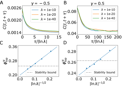
Figure 10: Model behavior with partially symmetric or antisymmetric interaction matrices. Even when the interaction matrix possesses some degree of symmetry or asymmetry, $\tau_{\lambda}=|\ln\lambda|$ is the only timescale controlling the dynamics when $\lambda\to 0^{+}$. We plot the collapse of the correlation function $C_{\lambda}(t,t+\tau)$ as a function of $\tau/\left|\ln\lambda\right|$ for partially anti-symmetric ($\gamma=-0.5$, A) and partially symmetric ($\gamma=0.5$, B) interaction matrices. The top diversity, measured at finite $\lambda$, asymptotically goes below the May bound as $\lambda\to 0^{+}$ for partially anti-symmetric ($\gamma=-0.5$, C) and partially symmetric ($\gamma=0.5$, D) interaction matrices. The diversity is evaluated by counting the number of species with $N_{i}>10^{-3}$. The form of the extrapolation in powers of $|\ln\lambda|$ is explained in Sec. A.4. Parameters: (A) $S=5000,\,\mu=10,\,\sigma=1.3$, average over 40 realizations (B) $S=5000,\,\mu=50,\,\sigma=4$ , average over 40 realizations.

We now consider the case $\gamma\neq 0$ in the limit $\lambda\to 0^{+}$. We generalize the previous argument connecting fluctuations, diversity and species turnover based on the many-body equations of motion and derive Eq. (14). We assume that the previous scaling for the timescale of the correlation matrix holds, which we check numerically, see Fig. 10. In other words, at any time $s=t/|\ln\lambda|$, the system is close to a fixed point, meaning that some species (a fraction $\phi_{{\rm top}}$ of them) are abundant and verify

$$1-N_{i}(s)-\sum_{j\neq i}\alpha_{ij}N_{j}(s)=0\,,$$

while the others are nearly extinct, i.e. asymptotically

$$N_{i}(s)=0\ .$$

Between $s$ and $s+\mathrm{d}s$ (where $\mathrm{d}s$ is an infinitesimal interval) we distinguish four types of populations: the ones that were extinct at $s$ but are present at $s+\mathrm{d}s$ (that we refer to as incoming species); the ones that are abundant at both $s$ and $s+ds$ (that we refer to as surviving species); the ones abundant at $s$ but rare at $s+\mathrm{d}s$ (that we refer to as extinct species); and finally the ones rare at both $s$ and $s+ds$ that do not play any role in the following argument. At time $s$, we have for the surviving species

$$1-N_{i}(s)-\sum_{j\neq i}^{\mathrm{surv}}\alpha_{ij}N_{j}(s)+\sum_{j}^{\mathrm{extinct}}\alpha_{ij}N_{j}(s)=0\,,$$

and correspondingly at time $s+\mathrm{d}s$,

$$1-N_{i}(s+\mathrm{d}s)-\sum_{j\neq i}^{\mathrm{surv}}\alpha_{ij}N_{j}(s+\mathrm{d}s)+\sum_{j}^{\mathrm{incoming}}\alpha_{ij}N_{j}(s+\mathrm{d}s)=0\,.$$

For all $i$ (where $i$ is a surviving species), we introduce the notations

$$\tilde{h}_{i}=\sum_{j}^{\mathrm{extinct}}\alpha_{ij}N_{j}(s)\,,$$

$$h_{i}=\sum_{j}^{\mathrm{incoming}}\alpha_{ij}N_{j}(s+\mathrm{d}s)\,.$$

Therefore, for the surviving species

$$\delta N_{i}\equiv N_{i}(s+\mathrm{d}s)-N_{i}(s)=(\mathrm{Id}+\boldsymbol{\alpha}^{*})_{ij}^{-1}(h_{j}-\tilde{h}_{j})\,,$$

where $\boldsymbol{\alpha}^{*}$ is $\boldsymbol{\alpha}$ reduced to the surviving species. We can now write the quadratic variation of the population sizes over all species

$$\lim_{\mathrm{d}s\to 0}\frac{1}{S}\sum_{i=1}^{s}\frac{\left(\delta N_{i}\right)^{2}}{\mathrm{d}s}=\lim_{\mathrm{d}s\to 0}\frac{1}{S}\sum_{i=1}^{\mathrm{surv}}\frac{\left(\delta N_{i}\right)^{2}}{\mathrm{d}s}+\lim_{\mathrm{d}s\to 0}\frac{1}{S}\sum_{i=1}^{\mathrm{extinct}}\frac{N_{i}(s)^{2}}{\mathrm{d}s}+\lim_{\mathrm{d}s\to 0}\frac{1}{S}\frac{1}{\mathrm{d}s}\sum_{i=1}^{\mathrm{incoming}}N_{i}(s+\mathrm{d}s)^{2}\,,$$

where we explicitly used the fact that for the incoming species $\delta N_{i}=N_{i}(s+\mathrm{d}s)$ and that $\delta N_{i}=-N_{i}(s)$ for the extinct ones. The number of incoming species scales as $O(\mathrm{d}s)$ and for them $N_{j}(s+\mathrm{d}s)\sim O(1)$ owing to the jump dynamics identified previously (for $\gamma=0$). Therefore we expect the perturbing field induced by the incoming species to scale as

$$h_{i}\sim\sqrt{\mathrm{d}s}\,,$$

a result in agreement with the scaling $\delta g\sim\sqrt{\mathrm{d}s}$ used in the previous section. Therefore, the species going extinct between $s$ and $s+\mathrm{d}s$ must at time $s$ have a population size of the order of $N_{i}(s)\sim\sqrt{\mathrm{d}s}$. As a consequence,

$$\lim_{\mathrm{d}s\to 0}\frac{1}{S}\sum_{i=1}^{\mathrm{extinct}}\frac{N_{i}(s)^{2}}{\mathrm{d}s}=0\,,$$

because the fraction of extinct species scales as $O({\rm d}s).$ The perturbing field induced by the extinct species is thus much smaller than the one induced by the incoming ones,

$$\tilde{h}_{i}\sim\mathrm{d}s\,.$$

Lastly, for the surviving species, we have

$$\lim_{\mathrm{d}s\to 0}\frac{1}{S}\sum_{i=1}^{\mathrm{surv}}\frac{\left(\delta N_{i}\right)^{2}}{\mathrm{d}s}=\lim_{\mathrm{d}s\to 0}\frac{1}{S}\sum_{i=1}^{\mathrm{surv}}\sum_{j,k}^{\mathrm{surv}}(\mathrm{Id}+\boldsymbol{\alpha}^{*})_{ij}^{-1}(\mathrm{Id}+\boldsymbol{\alpha}^{*})_{ik}^{-1}\frac{h_{j}h_{k}}{\mathrm{d}s}\,.$$

Based on the DMFT analysis of the $\gamma=0$ case, we assume that the $O(\sqrt{\mathrm{d}s})$ perturbing fields $h_{j}$ are statistically independent of the state of the system at time $s$ and that to leading order in $\mathrm{d}s$, $h_{j},h_{k}$ are uncorrelated for $j\neq k$. Therefore we obtain,

$$\lim_{\mathrm{d}s\to 0}\frac{1}{S}\sum_{i=1}^{\mathrm{surv}}\frac{\left(\delta N_{i}\right)^{2}}{\mathrm{d}s}=\lim_{\mathrm{d}s\to 0}\left(\frac{1}{S}\sum_{i}\frac{h_{i}^{2}}{\mathrm{d}s}\right)\frac{\phi_{{\rm top}}}{S^{*}}\mathrm{Tr}\left[(\mathrm{Id}+\boldsymbol{\alpha}^{*})^{-1}\left((\mathrm{Id}+\boldsymbol{\alpha}^{*})^{-1}\right)^{t}\right]\,.$$

We furthermore assume that to compute the trace we can take $\boldsymbol{\alpha}^{*}$ to be sampled from the same ensemble as the full interaction matrix $\alpha$ (albeit with a smaller size), neglecting the correlations induced by the dynamical selection of the community of surviving species. Relying on the cavity method, the validity of this approximation has been argued in the fixed point phase [13, 45] and more generally at the level of the average spectral density, see [35] (the possible existence of two outlying eigenvalues [45] is sub-extensive in the trace). We thus have,

$$\frac{1}{S^{*}}\mathrm{Tr}\left[(\mathrm{Id}+\boldsymbol{\alpha}^{*})^{-1}\left((\mathrm{Id}+\boldsymbol{\alpha}^{*})^{-1}\right)^{t}\right]=\left[\left(\frac{1+\sqrt{1-4\gamma\phi_{{\rm top}}\sigma^{2}}}{2}\right)^{2}-\phi_{{\rm top}}\sigma^{2}\right]^{-1}\,.$$

Furthermore,

$$\lim_{\mathrm{d}s\to 0}\left(\frac{1}{S}\sum_{i}\frac{h_{i}^{2}}{\mathrm{d}s}\right)=\lim_{\mathrm{d}s\to 0}\left(\frac{\sigma^{2}}{S\mathrm{d}s}\sum_{i=1}^{\mathrm{incoming}}N_{i}(s+\mathrm{d}s)^{2}\right)\,.$$

Together, we obtain

$$2\left|\hat{C}^{\prime}\left(0^{+}\right)\right| =\left(1+\phi_{{\rm top}}\sigma^{2}\left[\left(\frac{1+\sqrt{1-4\gamma\phi_{{\rm top}}\sigma^{2}}}{2}\right)^{2}-\phi_{{\rm top}}\sigma^{2}\right]^{-1}\right)\lim_{\mathrm{d}s\to 0}\left(\frac{1}{S\mathrm{d}s}\sum_{i=1}^{\mathrm{incoming}}N_{i}(s+\mathrm{d}s)^{2}\right)\,,$$

$$=\frac{\left(1+\sqrt{1-4\gamma\phi_{{\rm top}}\sigma^{2}}\right)^{2}}{\left(1+\sqrt{1-4\gamma\phi_{{\rm top}}\sigma^{2}}\right)^{2}-4\phi_{{\rm top}}\sigma^{2}}\lim_{\mathrm{d}s\to 0}\left(\frac{1}{S\mathrm{d}s}\sum_{i=1}^{\mathrm{incoming}}N_{i}(s+\mathrm{d}s)^{2}\right)\,.$$

Hence, we recover Eq. (14) of the main text

$$2|\hat{C}^{\prime}\left(0^{+}\right)|=\frac{\left(1+\sqrt{1-4\gamma\phi_{{\rm top}}\sigma^{2}}\right)^{2}}{\left(1+\sqrt{1-4\gamma\phi_{{\rm top}}\sigma^{2}}\right)^{2}-4\phi_{{\rm top}}\sigma^{2}}G\,,$$ (23)

with

$$G=\lim_{\mathrm{d}s\to 0}\frac{1}{S\mathrm{d}s}\sum_{i\in\mathcal{I}(s,s+{\rm d}s)}N_{i}(s+{\rm d}s)^{2}\,,$$

and where $\mathcal{I}(s,s+{\rm d}s)$ is the subset of species experiencing a jump from rare during the interval $[s,s+{\rm d}s]$. For $\gamma=0$, Eq. (23) reduces to Eq. (21) derived within the DMFT formalism.Additional figures and details for the Disscussion section

A.5 Convergence with $S$ and $\lambda$

Fig. 11, presents the convergence of $\left\langle N\right\rangle,\left\langle N^{2}\right\rangle$, showing that it is quantitatively quite robust to changes in $\lambda,S$. One implication is that other definitions of diversity besides than species richness, will be quite robust. For example, defining diversity using the inverse Simpson index $S^{-1}\left(\sum_{i}N_{i}\right)^{2}/\sum_{i}N_{i}^{2}$ that is approximately $\left\langle N\right\rangle^{2}/\left\langle N^{2}\right\rangle$, is relatively robust in $S,\lambda$, due to the robustness of $\left\langle N\right\rangle,\left\langle N^{2}\right\rangle$.

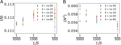
Figure 11: Behavior of the first and second moments of the population size. $\left\langle N\right\rangle$ and $\left\langle N^{2}\right\rangle$ are robust predictions that weakly depend on the number of species $S$ and the migration rate $\lambda$. In the inspected range of parameters, the variations in $\left\langle N\right\rangle$ are of the order of 1% and those in $\left\langle N^{2}\right\rangle$ of the order of 10%. Parameters: $\sigma=1.8$, $\mu=10$, average over 80 realizations.

As briefly discussed in Sec. VIII, to measure $\phi_{{\rm top}}$ at finite $S$ and $\lambda$, we test two options. The first is simply a threshold on the abundance: counting all the species with $N_{i}\geq\epsilon$ at a given time, for some chosen $\epsilon\ll 1$. Let $\phi_{{\rm top}}^{\text{N}}(S,\lambda,\epsilon)$ be the diversity measured this way. The second measure, denoted by $\phi_{{\rm top}}^{\text{g}}(S,\lambda,\epsilon)$, utilizes the invasion growth rate $g_{i}$. In it, in addition to $N_{i}\geq\epsilon$ we also requires $g_{i}>0$. For both measures, we find a similar form for the dependence on $\lambda,S,\epsilon$. For $\phi_{{\rm top}}^{\text{N}}$,

$$\phi_{{\rm top}}^{\text{N}}(S,\lambda,\epsilon)=\phi_{{\rm top}}+c_{1}\left|\ln\lambda\right|^{-\beta_{\text{N}}}+c_{2}/S+A\epsilon\,.$$ (24)

where $A=P(N=0^{+})$, $c_{1,2}$ are constants, and the exponent $\beta_{\text{N}}=1/2$. The expression for $\phi_{{\rm top}}^{\text{g}}$ is of the same form, only with $\beta_{\text{g}}=1$. This form of convergence can be understood as follows. We find that the asymptotic distribution $P(z)$ diverges as $(-z)^{-1/2}$ when $z\to 0^{-}$. This can be traced back to the fact that $\dot{z}=0$ when $z(s)$ leaves the confining wall. Therefore, by defining a cutoff $N\geq\epsilon$, or equivalently $z\geq\ln\epsilon/|\ln\lambda|$, the error made in sampling the distribution $P(z)$ for $z<0$ scales as $\sqrt{|\ln\epsilon/\ln\lambda|}$, hence the result in Eq. (24). However, when conditioned on $g>0$, the distribution $\mathbb{P}(g>0,z)$ is found to be finite when $z\to 0^{-}$ stemming from the fact that $\dot{z}>0$ when $z(s)$ reaches the wall from below. Thus, by defining a cutoff $N\geq\epsilon$, or equivalently $z\geq\ln\epsilon/|\ln\lambda|$, the error made in sampling the distribution $\mathbb{P}(g>0,z)$ for $z<0$ only scales as $|\ln\epsilon/\ln\lambda|$, hence the exponent $\beta_{\text{g}}=1$. These properties of the steady-state distribution $\mathbb{P}(g,z)$ seem to be robust features of persistent random walkers confined by hard obstacles and have been discussed in other contexts [46, 47, 48]. Since in practice $\left|\ln\lambda\right|$ would not be a very large number, the difference in the convergence in $\lambda$ is important. Quantitatively, $\phi_{{\rm top}}^{\text{N}},\phi_{{\rm top}}^{\text{g}}$ are typically larger than $\phi_{{\rm top}}$, and the convergence in $\lambda$ of $\phi_{{\rm top}}^{\text{g}}$ is indeed much faster, again highlighting the relevance of $g$. We find that the measure $\phi_{{\rm top}}^{\text{N}}(S,\lambda,\epsilon)$ is often above the stability bound, in contrast to the asymptotic $\phi_{{\rm top}}$ which is always below it. $\phi_{{\rm top}}^{\text{g}}(S,\lambda,\epsilon)$ can be either above or below this bound, depending on the parameters, see Fig. 6.

A.6 Identifying top species by selection and subsequent dynamics

The separation of top species from the rest is guaranteed for $\lambda\to 0^{+}$. Yet as discussed in Sec. VII, for finite $S,\lambda$ this separation is not very clear when looking at the abundances, see $P(N)$ in Fig. 4(A). By using insights gleaned from the theory, we have shown, see Sec. VII and Fig. 6, that this separation can be much better defined even away from the asymptotic limit, by also considering $g_{i}$, the invasion growth rate defined in Sec. III.1. Here we show, that if we can manipulate the system, by removing certain judiciously-chosen species and rerunning the dynamics, the asymptotic distribution $P(N)$ can be remarkably well reproduced at reasonable $S,\lambda$. Beyond potential applications to experiments, this seems to suggest that the separation between abundant species and the others is still present, even when it seems blurred with other measures.

The lack of clear separation is most pronounced at not-very-small $N$ (say $N\sim 0.1$). There, one finds: (1) abundant species, (2) species that grow from rare and are about to disrupt the abundant species, and (3) species with negative growth rate that are leaving the abundant subset. The abundant species (group 1) are characterized by appreciable $N$, and being at a fixed point, $g\simeq N$. They occupy an equilibrium that is fully stable if not disrupted by species that grow from rare (group 2). These can have significant $g$, with still $N$ small compared to $g$. The idea here is to remove species (2) and (3), which we do by removing all species that have $N_{i}/g_{i}<1/2$, corresponding to species with positive growth rate that are in the midst of their jump, below halfway, and those with negative growth rate in Fig. 3,7. Then, we run again the dynamics, and we find that the remaining species reach a stable equilibrium. The properties of the equilibrium obtained in this way are remarkably similar to those predicted by the asymptotic theory, even for reasonable $\lambda$. Fig. 13 shows the obtained abundance distribution $P(N)$. It is similar to the asymptotic distribution, and in contrast quite different from the instantaneous unfiltered $P(N)$ from Fig. 4(A). Furthermore, the resulting distribution is distinct from those in the fixed point phase (when $\sigma<\sqrt{2}$), as shown by a comparison with the predicted distribution there, a truncated Gaussian. The asymptotic species richness $\phi_{\text{top}}=0.28$ is recovered within 1%; this is lower than the stability bound, at $\phi=0.31$.

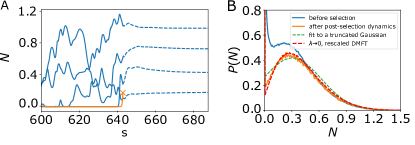
Figure 13: Identifying the top species by combined selection and dynamics. (A) Top species are identified by stopping the dynamics (solid lines), and removing species that are about to grow and disrupt the system, here the orange trajectory, and those with a negative invasion growth rate (by removing species $i$ if $N_{i}/g_{i}<1/2$), and then continuing the dynamics (dashed lines). The outcome is an equilibrium. (B) The distribution of abundances thus obtained is close to the asymptotic distribution obtained from the rescaled dynamics. It is much closer than the bare abundance distribution $P(N)$, and is also very different from the distribution in the equilibrium phase. $S=5000$, $\sigma=1.8$, $\mu=10$, $\lambda=10^{-10}$.

Numerical methods

Here we detail the numerical procedures used in producing the figures. They are of two types:

(1) Full many-variable simulations of Eq. (1).

(2) Numerical solution of the rescaled dynamics, defined in full in Eqs. (5,7,8).

(1) We used the explicit Runge-Kutta method of order 5(4) implemented by the ODE solver scipy.solve_ivp in Python, to simulate Eq. (1).

(2) The set of equations of the rescaled dynamics are self-consistent: the trajectory $z(s)$ depends on $g(s)$, which is sampled with correlation function $\hat{C}(s,s^{\prime})$ and mean $m(s)$. Self-consistently, $\hat{C}(s,s^{\prime}),\,m(s)$ depend on the statistics of $z(s)$, see Eqs. (7,8). This self-consistency is standard in DMFT formulations. We used a well-known numerical method to solve it [49, 16]. It starts with a guess for $\left\langle g(s)g(s^{\prime})\right\rangle,\,\left\langle g(s)\right\rangle,$ generates realizations of $g(s)$ and from that trajectories $z(s)$, which are then used to update $\left\langle g(s)g(s^{\prime})\right\rangle,\,\left\langle g(s)\right\rangle$. This is repeated until convergence.

In practice, the DMFT simulations were carried with: a timestep ${\rm d}s=0.5$ for $s<500$, ${\rm d}s=0.1$ for $500\leq s<600$ and ${\rm d}s=0.05$ for $600\leq s<700$. We used (i) 500 iterations with averaging over 1000 realizations and injection fraction $0.3$ followed by (ii) 1000 iterations with averaging over 10000 realizations and injection fraction $0.3$ followed by (iii) 1500 iterations with averaging over 10000 realizations and injection fraction $0.03$ and followed by (iv) 2000 iterations with averaging over 10000 realizations and injection fraction $0.003$. In order to precisely obtain the diversity graph in Fig. 1(G) we initialized the algorithm with $\left\langle g(s)g(s^{\prime})\right\rangle,\,\left\langle g(s)\right\rangle$ given by their fixed point branch value with $\left\langle g(s)g(s^{\prime})\right\rangle$ destabilized by a small identity matrix (corresponding to small amplitude white noise). The results agree very well with the asymptotic values found from full simulations of Eq. (1), when $S\to\infty,\lambda\to 0^{+}$ are taken carefully, see Fig. 6.

Simulation details for individual figures of the main text:

Fig. 1. (A) $S=1000$, $\sigma=1$, $\mu=10$, $\lambda=10^{-8}$ (B) $S=1000$, $\sigma=2$, $\mu=10$, $\lambda=10^{-8}$ (C, E) $S=20000$, $\sigma=1$, $\mu=10$, average over 200 realizations. (D, F) $S=20000$, $\sigma=2$, $\mu=10$, average over 200 realizations. (G) DMFT numerics of the rescaled equation at $\mu=10$.

Fig. 2: (A) $S=5000$, $\lambda=10^{-10}$, $\sigma=2$, $\mu=10$. (B) $S=20000$, $\lambda=10^{-10}$, $\sigma=2$, $\mu=10$, average over 40 realizations (C) $S=20000$, $\lambda=0$, $\sigma=2$, $\mu=10$, average over 40 realizations. (D) $S=20000$, $\sigma=2$, $\mu=10$, average over 40 realizations. DMFT line obtained with the $\lambda\to 0^{+}$ rescaled dynamics.

Fig. 4: same as in Fig. 2. (A,C) $S=20000$, $\lambda=0$, $\sigma=2$, $\mu=10$, average over 40 realizations. DMFT line obtained with the $\lambda=0$ rescaled dynamics. (B, D) $S=20000$, $\sigma=2$, $\mu=10$, average over 40 realizations. DMFT line obtained with the $\lambda\to 0^{+}$ rescaled dynamics.

Fig. 5: Same as in Fig. 2. S=20000, $\sigma=2$, $\mu=10$, average over 40 realizations. All species start at $N_{i}(t=0)=0.5$.

Fig. 6: $\sigma=1.8$, $\mu=10$, average over 40 realizations.

Fig. 7: $S=5000$, $\sigma=1.8$, $\mu=10$, $\lambda=10^{-6}$.

References

- [1] Elisa Benincà, Bill Ballantine, Stephen P. Ellner, and Jef Huisman. Species fluctuations sustained by a cyclic succession at the edge of chaos. Proceedings of the National Academy of Sciences, 112(20):6389–6394, May 2015.
- [2] Gregor F. Fussmann, Stephen P. Ellner, Kyle W. Shertzer, and Nelson G. Hairston Jr. Crossing the Hopf Bifurcation in a Live Predator-Prey System. Science, 290(5495):1358–1360, November 2000.
- [3] G. F. Gause. Experimental Analysis of Vito Volterra’s Mathematical Theory of the Struggle for Existence. Science, 79(2036):16–17, January 1934.
- [4] Josef Hofbauer and Karl Sigmund. Evolutionary Games and Population Dynamics. Cambridge university press, 1998.
- [5] Jacopo Grilli. Macroecological laws describe variation and diversity in microbial communities. Nature Communications, 11(1):4743, December 2020.
- [6] Enrico Ser-Giacomi, Lucie Zinger, Shruti Malviya, Colomban De Vargas, Eric Karsenti, Chris Bowler, and Silvia De Monte. Ubiquitous abundance distribution of non-dominant plankton across the global ocean. Nature ecology & evolution, 2(8):1243–1249, 2018.
- [7] Antonio M. Martin-Platero, Brian Cleary, Kathryn Kauffman, Sarah P. Preheim, Dennis J. McGillicuddy, Eric J. Alm, and Martin F. Polz. High resolution time series reveals cohesive but short-lived communities in coastal plankton. Nature Communications, 9(1):266, December 2018.
- [8] J. Cesar Ignacio-Espinoza, Nathan A. Ahlgren, and Jed A. Fuhrman. Long-term stability and Red Queen-like strain dynamics in marine viruses. Nature Microbiology, 5(2):265–271, February 2020.
- [9] Vincent Miele, Rodrigo Ramos-Jiliberto, and Diego P Vázquez. Core–periphery dynamics in a plant–pollinator network. Journal of Animal Ecology, 89(7):1670–1677, 2020.
- [10] Mark R Gardner and W Ross Ashby. Connectance of large dynamic (cybernetic) systems: critical values for stability. Nature, 228(5273):784–784, 1970.
- [11] Robert M. May. Will a large complex system be stable? Nature, 238(5364):413–414, 1972.
- [12] Manfred Opper and Sigurd Diederich. Phase transition and 1/f noise in a game dynamical model. Physical review letters, 69(10):1616, 1992.
- [13] Guy Bunin. Ecological communities with Lotka-Volterra dynamics. Physical Review E, 95(4), April 2017.
- [14] Jiliang Hu, Daniel R. Amor, Matthieu Barbier, Guy Bunin, and Jeff Gore. Emergent phases of ecological diversity and dynamics mapped in microcosms. Science, 378(6615):85–89, October 2022.
- [15] David A. Kessler and Nadav M. Shnerb. Generalized model of island biodiversity. Physical Review E, 91(4):042705, 2015.
- [16] F Roy, G Biroli, G Bunin, and C Cammarota. Numerical implementation of dynamical mean field theory for disordered systems: Application to the Lotka–Volterra model of ecosystems. Journal of Physics A: Mathematical and Theoretical, 52(48):484001, November 2019.
- [17] Felix Roy, Matthieu Barbier, Giulio Biroli, and Guy Bunin. Complex interactions can create persistent fluctuations in high-diversity ecosystems. PLOS Computational Biology, 16(5):e1007827, May 2020.
- [18] Michael T. Pearce, Atish Agarwala, and Daniel S. Fisher. Stabilization of extensive fine-scale diversity by ecologically driven spatiotemporal chaos. Proceedings of the National Academy of Sciences, 117(25):14572–14583, June 2020.
- [19] Robert M. May and Warren J. Leonard. Nonlinear aspects of competition between three species. SIAM Journal on Applied Mathematics, 29(2):243–253, 1975.
- [20] Jacob D. O’Sullivan, J. Christopher D. Terry, and Axel G. Rossberg. Intrinsic ecological dynamics drive biodiversity turnover in model metacommunities. Nature Communications, 12(1):3627, June 2021.
- [21] Thibaut Arnoulx de Pirey and Guy Bunin. Aging by Near-Extinctions in Many-Variable Interacting Populations. Physical Review Letters, 130(9):098401, February 2023.
- [22] Kenneth J Locey and Jay T Lennon. Scaling laws predict global microbial diversity. Proceedings of the National Academy of Sciences, 113(21):5970–5975, 2016.
- [23] Sandro Azaele, Samir Suweis, Jacopo Grilli, Igor Volkov, Jayanth R. Banavar, and Amos Maritan. Statistical mechanics of ecological systems: Neutral theory and beyond. Reviews of Modern Physics, 88(3):035003, July 2016.
- [24] Alan Hastings. Timescales, dynamics, and ecological understanding. Ecology, 91(12):3471–3480, 2010.
- [25] L. F. Cugliandolo and J. Kurchan. Analytical solution of the off-equilibrium dynamics of a long-range spin-glass model. Physical Review Letters, 71(1):173–176, July 1993.
- [26] Jorge Kurchan and Laurent Laloux. Phase space geometry and slow dynamics. Journal of Physics A: Mathematical and General, 29(9):1929–1948, May 1996.
- [27] Robert May and Angela R McLean. Theoretical ecology: principles and applications. Oxford University Press, 2007.
- [28] Yasuhiro Takeuchi. Global dynamical properties of Lotka-Volterra systems. World Scientific, 1996.
- [29] Matthieu Barbier, Jean-François Arnoldi, Guy Bunin, and Michel Loreau. Generic assembly patterns in complex ecological communities. Proceedings of the National Academy of Sciences, 115(9):2156–2161, February 2018.
- [30] Joseph S Wright. Plant diversity in tropical forests: a review of mechanisms of species coexistence. Oecologia, 130:1–14, 2002.
- [31] Valentina Ros, Felix Roy, Giulio Biroli, Guy Bunin, and Ari M. Turner. Generalized Lotka-Volterra equations with random, non-reciprocal interactions: The typical number of equilibria, December 2022.
- [32] Itay Dalmedigos and Guy Bunin. Dynamical persistence in high-diversity resource-consumer communities. PLOS Computational Biology, 16(10):e1008189, October 2020.
- [33] Paul Marrow, Richard Law, and C. Cannings. The coevolution of predator—prey interactions : ESSS and Red Queen dynamics. Proceedings of the Royal Society of London. Series B: Biological Sciences, 250(1328):133–141, 1992.
- [34] Josef Hofbauer and Sebastian J. Schreiber. Permanence via invasion graphs: Incorporating community assembly into modern coexistence theory. Journal of Mathematical Biology, 85(5):54, October 2022.
- [35] Giulio Biroli, Guy Bunin, and Chiara Cammarota. Marginally stable equilibria in critical ecosystems. New Journal of Physics, 20(8):083051, August 2018.
- [36] Chen Liu, Giulio Biroli, David R Reichman, and Grzegorz Szamel. Dynamics of liquids in the large-dimensional limit. Physical Review E, 104(5):054606, 2021.
- [37] Haim Sompolinsky and Annette Zippelius. Relaxational dynamics of the Edwards-Anderson model and the mean-field theory of spin-glasses. Physical Review B, 25(11):6860, 1982.
- [38] Marc Mézard, Giorgio Parisi, and Miguel Virasoro. Spin Glass Theory and beyond: An Introduction to the Replica Method and Its Applications, volume 9. World Scientific Publishing Co Inc, 1987.
- [39] Elisabeth Agoritsas, Giulio Biroli, Pierfrancesco Urbani, and Francesco Zamponi. Out-of-equilibrium dynamical mean-field equations for the perceptron model. Journal of Physics A: Mathematical and Theoretical, 51(8):085002, February 2018.
- [40] For any process with time-translation invariant correlation , we have . Therefore is possible only if the increment scales as as for Brownian motion.
- [41] Markus Müller and Matthieu Wyart. Marginal Stability in Structural, Spin, and Electron Glasses. Annual Review of Condensed Matter Physics, 6(1):177–200, March 2015.
- [42] Alan Roberts. The stability of a feasible random ecosystem. Nature, 251:607–608, 1974.
- [43] Giulia Garcia Lorenzana and Ada Altieri. Well-mixed lotka-volterra model with random strongly competitive interactions. Physical Review E, 105(2):024307, 2022.
- [44] Emil Mallmin, Arne Traulsen, and Silvia De Monte. Chaotic turnover of rare and abundant species in a strongly interacting model community, 2023.
- [45] Matthieu Barbier, Claire de Mazancourt, Michel Loreau, and Guy Bunin. Fingerprints of High-Dimensional Coexistence in Complex Ecosystems. Physical Review X, 11(1):011009, January 2021.
- [46] Thibaut Arnoulx de Pirey and Frédéric van Wijland. A run-and-tumble particle around a spherical obstacle: steady-state distribution far-from-equilibrium. arXiv e-prints, pages arXiv–2303, 2023.
- [47] Caleb G Wagner, Michael F Hagan, and Aparna Baskaran. Steady-state distributions of ideal active brownian particles under confinement and forcing. Journal of Statistical Mechanics: Theory and Experiment, 2017(4):043203, apr 2017.
- [48] Barath Ezhilan, Roberto Alonso-Matilla, and David Saintillan. On the distribution and swim pressure of run-and-tumble particles in confinement. Journal of Fluid Mechanics, 781:R4, 2015.
- [49] H. Eissfeller and M. Opper. New method for studying the dynamics of disordered spin systems without finite-size effects. Physical Review Letters, 68(13):2094–2097, March 1992.