Optimal Vaccination Policy to Prevent Endemicity
A Stochastic Model

Abstract

We examine here the effects of recurrent vaccination and waning immunity on the establishment of an endemic equilibrium in a population. An individual-based model that incorporates memory effects for transmission rate during infection and subsequent immunity is introduced, considering stochasticity at the individual level. By letting the population size going to infinity, we derive a set of equations describing the large scale behavior of the epidemic. The analysis of the model’s equilibria reveals a criterion for the existence of an endemic equilibrium, which depends on the rate of immunity loss and the distribution of time between booster doses. The outcome of a vaccination policy in this context is influenced by the efficiency of the vaccine in blocking transmissions and the distribution pattern of booster doses within the population. Strategies with evenly spaced booster shots at the individual level prove to be more effective in preventing disease spread compared to irregularly spaced boosters, as longer intervals without vaccination increase susceptibility and facilitate more efficient disease transmission. We provide an expression for the critical fraction of the population required to adhere to the vaccination policy in order to eradicate the disease, that resembles a well-known threshold for preventing an outbreak with an imperfect vaccine. We also investigate the consequences of unequal vaccine access in a population and prove that, under reasonable assumptions, fair vaccine allocation is the optimal strategy to prevent endemicity.

Keywords: age-structured model; endemicity; waning immunity; heterogeneous vaccination; varying infectiousness and susceptibility; mitigation; non-Markovian model; recurrent vaccination.

1 Introduction

In epidemiology, a disease is called endemic if it persists in a population over a long period of time. Many diseases are endemic in some parts of the world, including for instance malaria and tuberculosis (Hay et al., 2009; Oliwa et al., 2015), and several studies have proposed that endemicity is a likely outcome for the recent COVID-19 epidemic (Antia and Halloran, 2021; Lavine et al., 2021), as is currently the case for other human coronavirus-induced diseases (Su et al., 2016). The persistence of a disease in a population can incur a large cost for society and endemic diseases are responsible for a large share of the deaths from communicable diseases every year. Understanding the mechanisms underlying the establishment of such an endemic state and how to control it is therefore of great public health importance. Prophylactic vaccination, when available, is a common and efficient way to mitigate the spread of diseases (Plotkin, 2005; Rashid et al., 2012). If the vaccine blocks part of the transmissions, a high enough vaccine coverage can prevent self-sustained transmissions in the population, leading to a so-called herd immunity (Anderson and May, 1985; Fine et al., 2011; Randolph and Barreiro, 2020). This phenomenon has been the subject of a large body of work in the mathematical modeling literature, aimed at informing policy-makers on the effectiveness of a vaccination campaign and at developing a theoretical understanding of the epidemiological consequences of vaccination. An important achievement of these studies is the derivation of an expression for the critical vaccine coverage required to eradicate a disease, under various scenarios of increasing complexity (Anderson and May, 1982; Farrington, 2003; Magpantay, 2017; Delmas et al., 2022). However, the bulk of this work pertains to vaccines providing life-long (or slowly waning) immunity and administrated at birth or at a single point in time. Although these assumptions might represent adequately many situations (including for instance childhood diseases), infection by some pathogens and vaccines are known to provide no or temporary immunity (Vynnycky and Fine, 1997; RTS, 2015; Stein et al., 2023). An important motivating example for our work is the recent COVID-19 epidemic, for which re-infections after either primary infection or vaccination have been reported (Stein et al., 2023), and for which direct measurements of several components of adaptive immunity suggest that part of it is waning (Shrotri et al., 2022; Lin et al., 2022). The understanding of the impact of vaccination under such short-lived immunity remains limited and motivates further theoretical developments.

In this work, we consider a pathogen for which a vaccine that blocks transmissions is available but with an immunity that wanes with time, both for individuals infected and vaccinated. Although our main motivation is COVID-19, we consider a generic disease with these two features. As the immunity conferred by the vaccine is temporary, the effect of a single vaccination rapidly fades and herd immunity can only be achieved (and thus an endemic state prevented) if individuals are vaccinated recurrently (Randolph and Barreiro, 2020). However, even recurrent vaccination might fail to provide herd immunity. Under recurrent vaccination, the level of immunity in the population is shaped by two antagonistic forces: boosting due to vaccine injections and re-exposure to the pathogen, and waning due to decay in circulating antibody levels and/or memory cells. If vaccination is too scarce or immunity decays too rapidly, the vaccine-induced immunity might not block enough transmissions to prevent the disease from spreading in the population and reaching endemicity. What drives the outcome of a vaccination policy is therefore a complex interplay between the transmissibility of the disease, the waning of the immunity (which sets up the time scale after which re-infection can occur) and the frequency of immune boosting by vaccines. We investigate this effect by constructing an epidemic model that incorporates both waning immunity and recurrent vaccination, and by analysing how these two components interact to determine the long-term establishment of the disease.

In standard SIR-type models, waning immunity can be modeled by letting the infected individuals go back to a susceptible state, either directly after the infection as in the SIS model, or after a temporary immune period as in the SIRS model (Brauer et al., 2019). Extensions of these models where the duration of the immune period is fixed or has a general distribution have also been proposed, for instance in Hethcote et al. (1981); Cooke and Van Den Driessche (1996); Taylor and Carr (2009); Bhattacharya and Adler (2012). In such models, immunity is lost instantaneously as individuals go from being fully protected (in the $R$ state) to being fully susceptible to the disease (in the $S$ state). Some studies consider a more gradual loss of immunity by adding one or several intermediate compartments with partial immunity, often denoted by $W$ (for waning) (Lavine et al., 2011; Carlsson et al., 2020). In our work, we will model the decay of immunity by tracking for each individual a susceptibility giving the probability of being re-infected upon exposure to the pathogen. Waning immunity is modeled by having the susceptibility increase with time following an infection or vaccination, with no further assumption. This approach can account for the situations described above, where each individual is in one of finitely many immune states ($R$, $S$, $W$), but also for a continuous loss of immunity. The idea of modeling a susceptibility dates back to the endemic models of Kermack and McKendrick (Kermack and McKendrick, 1932, 1933), see also Inaba (2001); Breda et al. (2012) for modern formulations, and is also reminiscent of existing works describing immunity as a continuous variable (White and Medley, 1998; Diekmann et al., 2018; Barbarossa and Röst, 2015; Martcheva and Pilyugin, 2006). Modeling immunity through an abstract susceptibility is a phenomenological approach, but mechanistic approaches have also been proposed. These require to model explicitly for each individual some components of the immune system (T-cells, B-cells, antibodies, cytokines, …) and their interaction with the pathogen, as for instance in Heffernan and Keeling (2008, 2009); Goyal et al. (2020); Néant et al. (2021). Such an approach is both more realistic and opens the possibility of being calibrated using clinical data (Lin et al., 2022), but adds a new layer of complexity (the within-host dynamics) which can be cumbersome for theory purpose. We will think of our susceptibility as aggregating the effect of this complicated within-host process.

The effect of immune boosting through recurrent vaccination has also drawn attention from modelers (Arino et al., 2003; Lavine et al., 2011; Carlsson et al., 2020; Leung et al., 2018). Let us note that, in the vaccination strategy that we consider, individuals are vaccinated recurrently during their lifetime, each at different moments. The name “continuous vaccination” has also been proposed for this type of vaccination (Liu et al., 2008; Li and Yang, 2011). This is different for instance of the “pulse vaccination strategy”, considered in Agur et al. (1993) in the context of measles, and that has received further attention (Liu et al., 2008; Li and Yang, 2011). In this strategy, at several fixed moments a fraction of the population is vaccinated, all individuals in a given vaccination pulse receiving their dose at the same time. Typically, recurrent boosting is modeled by letting individuals get vaccinated at a given rate (that can depend on age or other factors) in which case they are moved to a compartment with a reduced susceptibility. A notable difference with our work is that, in our model, the vaccination rate depends on the time elapsed since the previous vaccination. This reflects the fact that, at the microscopic level, we let the period of time between two consecutive vaccinations have a general (non-exponential) distribution. We have several motivations for relaxing the usual constant rate assumption. First, the resulting dynamics is much richer and complex. It encompasses more realistic situations that cannot be modeled using a constant rate, for instance the enforcement of a minimal duration between two vaccine doses, or the existence of a typical duration between two doses, leading to a peak in the distribution of this duration. Second, summarizing the effect of vaccination and waning immunity by a small number of parameters (the transition rates between the various immune compartments) obscures the role played by the exact shapes of the immunity decay and of the distribution between vaccine doses and leads to quite opaque expressions. For instance, if immunity following vaccination first plateaus and is then lost rapidly around a typical time, we expect a population where boosting occurs right before this time to build a much stronger immunity than if boosting occurred right after this time, although there is only a minimal variation in the overall vaccination rate. This type of effect cannot be studied by assuming that all durations have exponential distributions. From a mathematical point of view, this more general model requires to work with partial differential equations describing the “age structure” of the population rather than with more usual sets of ordinary differential equations. It is always interesting to note that similar age-structured epidemic models were used as early as in the foundational work of Kermack and McKendrick (Kermack and McKendrick, 1927), and that the compartmental SIR model was only introduced as a particular case of this more general dynamics.

Our model has one last specificity compared to more classical approaches based on compartments. It is formulated as an individual-based stochastic model from which we derive a set of deterministic equations describing its scaling limit (as the population size goes to infinity). Modeling the population at the microscopic level rather than directly at the continuum gives a better understanding of the hypotheses underlying the model, as well as a more transparent interpretation of the parameters as individual quantities. Moreover, in our model, part of this stochasticity will remain in the limit (through a conditioning term) which could have been easily missed if this convergence step was not carried out. Similar laws of large numbers have been obtained frequently in the probabilistic literature on population models (Kurtz, 1981; Oelschlager, 1990; Fournier and Méléard, 2004), in particular in an epidemic context (Clémençon et al., 2008; Barbour and Reinert, 2013; Britton et al., 2019; Pang and Pardoux, 2021; Foutel-Rodier et al., 2022). Our model draws inspiration from recent works on similar non-Markovian epidemics (Pang and Pardoux, 2021; Forien et al., 2021; Foutel-Rodier et al., 2022; Duchamps et al., 2021), and the limiting equations we obtain are connected to classical time-since-infection models in epidemiology (Diekmann, 1977; Diekmann et al., 1995).

Lastly, we would like to acknowledge the work of Forien et al. (2022), who consider a model very similar to ours (but without explicit vaccination), derive rigorously the scaling limit of the epidemic, and give criteria for the existence and asymptotic stability of an endemic equilibrium. We emphasize that, despite the striking similarities, the two models were formulated independently and most of the results presented in our work were obtained before that in Forien et al. (2022) were made available. Moreover, the main aim of our work is to draw public health insights from our model, letting sometimes mathematical rigour aside, whereas that of Forien et al. (2022) is mathematically much more accomplished and is targeted to an audience of probabilists. We believe that the two approaches offer complementary perspectives on the problem of waning immunity and endemicity.

The rest of this article is organized as follows. We start by describing our stochastic model and its large population size limit in Section 2. Then, in Section 3, we study the long-time behavior of the limiting equations and provide a simple criterion for the existence of an endemic equilibrium. In the final two sections, we examine the dependence of this criterion on the vaccination parameters to draw some public health insights from our model. We start with a general discussion in Section 4, and consider two more specific applications in Section 5, which require us to make a straightforward extension of our model to multiple groups.

2 The model

2.1 Model description

The dynamics without vaccination.

We consider the spread of a disease in a closed population of fixed size $N$, started at some reference time $t=0$ at which the state of the epidemic is known. Each individual in the population is characterized by two random quantities that change through time: its infectiousness, giving the rate at which it transmits the disease, and its susceptibility, corresponding to the probability that it gets re-infected upon contact with an infected individual. Individuals are labeled by $i\in\{1,\dots,N\}$, and the infectiousness of individual $i$ at time $t$ is denoted by $\lambda^{N}_{i}(t)$ while its susceptibility is denoted by $\sigma^{N}_{i}(t)$. We start by describing the dynamics of the epidemic in the absence of vaccination, and then indicate how vaccines are included to the model. The typical evolution of the susceptibility and infectiousness of an individual is represented in Figure 1.

Figure 1: Typical evolution of the susceptibility $\sigma$ (in blue, on top) and infectiousness $\lambda$ (in red, below) of an individual.

Consider a focal individual $i$. In the absence of vaccination, it goes repeatedly through two states. An infectious state (denoted by $I$) where it cannot be infected but can spread the disease, with $\lambda^{N}_{i}(t)\geq 0$ and $\sigma^{N}_{i}(t)=0$. And a susceptible state (denoted by $S$), where it does not spread the disease but can be re-infected, with $\lambda^{N}_{i}(t)=0$ and $\sigma^{N}_{i}(t)\geq 0$. It is important to note that, since susceptibility and infectiousness are continuous quantities, the meaning of the $I$ and $S$ states is different from that in SIR models: an individual in the $I$ state can have $\lambda^{N}_{i}(t)=0$ and thus not be infectious, and an individual in the $S$ state can have $\sigma^{N}_{i}(t)=0$ and be protected from re-infection.

Upon infection, say at time $\tau$, it enters the $I$ state and samples a random function $\lambda\colon[0,T_{I})\to[0,\infty)$ according to a given distribution $\mathcal{L}_{\lambda}$. The length $T_{I}$ of the domain of $\lambda$ is random, and we think of it as being part of the definition of $\lambda$. The individual remains in the $I$ state for a time period of length $T_{I}$. During this period, it cannot get re-infected, and its infectiousness is described by the function $\lambda$, that is,

$$\forall a<T_{I},\quad\lambda^{N}_{i}(\tau+a)=\lambda(a),\quad\sigma^{N}_{i}(\tau+a)=0.$$

At time $\tau+T_{I}$, the individual leaves the $I$ state, it is said to recover from the disease.

Once an individual has recovered from the disease, here at time $\tau^{\prime}=\tau+T_{I}$, it cannot spread the disease anymore and acquires an immunity against re-infection that wanes. It enters the $S$ state. To model that immunity is waning, the focal individual samples an independent random susceptibility $\sigma\colon[0,\infty)\to[0,1]$ according to another given distribution $\mathcal{L}_{\sigma}$ on the set of non-decreasing functions. We define

$$\forall a\geq 0,\quad\lambda^{N}_{i}(\tau^{\prime}+a)=0,\quad\sigma^{N}_{i}(\tau^{\prime}+a)=\sigma(a).$$

The susceptibility gives the probability to be infected upon exposure to the disease. More precisely, individual $i$ gets re-infected at time $t$ at rate $\sigma^{N}_{i}(t)\Lambda^{N}(t)$ with

$$\forall t\geq 0,\quad\Lambda^{N}(t)\coloneqq\frac{1}{N}\sum_{i=1}^{N}\lambda^{N}_{i}(t).$$ (1)

When such an event occurs, individual $i$ goes back to the $I$ state and we reproduce the above two steps independently. Note that since $\sigma^{N}_{i}(t)=0$ when $i$ is in state $I$, only susceptible individuals can be re-infected. The interpretation of the latter expression is that each infectious individual, at a rate proportional to its infectiousness, makes a contact targeted to an individual chosen uniformly in the population. This contact leads to an infection with a probability given by the susceptibility of the target individual.

Recovering the SIRS model.

Let us rapidly illustrate how to recover the usual compartmental models from the previous definitions. Suppose that $\lambda$ and $\sigma$ are given by

$$\forall a<T_{I},\quad\lambda(a)=\beta,\qquad\forall a\geq 0,\quad\sigma(a)=\mathbf{1}_{\{a\geq T_{R}\}}$$

where $T_{I}$ is exponentially distributed with parameter $\gamma$, and $T_{R}$ is a random variable giving the length of the immune period. Then, infectious individuals yield new infections at a constant rate $\beta$, and stop being infectious (that is, recover) at rate $\gamma$. After having recovered, an individual is completely immune to re-infections ($\sigma(a)=0$) for a random duration $T_{R}$, after which it becomes fully susceptible ($\sigma(a)=1$). Depending on the distribution of $T_{R}$, we can recover either the SIR, SIS or SIRS model. If $T_{R}=\infty$ a.s., individuals are permanently immune following an infection and our model becomes a stochastic version of the SIR model. If $T_{R}=0$ a.s., individuals build no immunity following an infection, and this corresponds to a stochastic SIS model. Finally, a stochastic SIRS model can be obtained by letting $T_{R}$ be exponentially distributed. Obviously, our model can account for much more complex situations, where infectiousness varies during the infectious period, and immunity is gradually lost following infection.

Adding vaccines.

The previous rules describe the dynamics of the epidemic in the absence of vaccination. We model vaccines by assuming that vaccination has the same effect as (natural) immunization by the disease: upon vaccination the susceptibility of an individual is “reset” to a new independent random curve $\sigma^{\prime}$ with law $\mathcal{L}_{\sigma}$, as if it had entered the $S$ state after having recovered from the disease. More formally, if $\tau^{\prime\prime}$ denotes a (random) time at which $i$ is vaccinated, we set

$$\forall a\geq 0,\quad\lambda^{N}_{i}(\tau^{\prime\prime}+a)=0,\quad\sigma^{N}_{i}(\tau^{\prime\prime}+a)=\sigma^{\prime}(a).$$

for an independent random variable $\sigma^{\prime}$ with distribution $\mathcal{L}_{\sigma}$. We further assume that, as long as they are susceptible, individuals get vaccinated recurrently according to an independent renewal process with waiting period distribution $\mathcal{L}_{V}$. After having recovered from the disease, an individual will receive a vaccine dose after an independent period of random length $T_{V}$ distributed according to $\mathcal{L}_{V}$, unless it is re-infected by that time. If it gets vaccinated before being re-infected, it waits for a new period of independent length with distribution $\mathcal{L}_{V}$ before receiving a second vaccine dose. This process goes on until the individual is re-infected and goes back to the $I$ state.

The dynamics of the population can be obtained by carrying out the previous steps altogether for each of the $N$ individuals. Every time an individual is affected by an event (recovery, infection, vaccination), it samples its new susceptibility or infectiousness independently of all other individuals and of the past dynamics, according to $\mathcal{L}_{\lambda}$ in case of an infection or $\mathcal{L}_{\sigma}$ otherwise. A formal construction of the epidemic is carried out in Appendix A.1. Overall, apart from the initial condition, the dynamics of the epidemic depends on four parameters: the population size $N$, the distribution of the infectiousness curve $\mathcal{L}_{\lambda}$, the distribution of the susceptibility curve $\mathcal{L}_{\sigma}$ and the distribution of the duration between two vaccinations $\mathcal{L}_{V}$. We will always assume that $T_{I}$ and $T_{V}$ have a density and a finite expectation. Some realizations of the model are displayed in Figure 2.

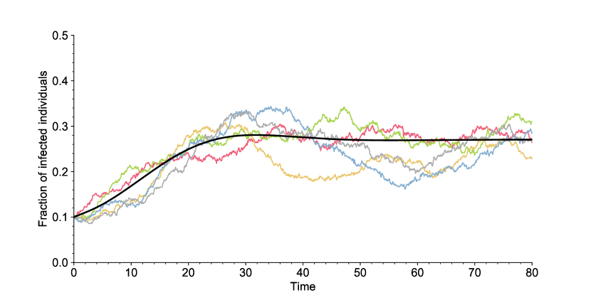
Figure 2: Independent simulations of the model (colored lines) for $N=500$ and of its deterministic limit, as $N\to\infty$ (solid black line). All parameter values are given in Table 1 (Section A.6). The simulations are initialized with a fraction $I_{0}=0.1$ of infectious individuals.

Population age structure.

Since the infectiousness and susceptibility are varying with time in our model, the state of the epidemic is not accurately described by counting the number of infectious and susceptible individuals. Deriving the large population size limit of the model requires to record for each individual a duration, which is the time elapsed since the last event (infection, recovery, or vaccination) that they experienced. We refer to this duration as the class age, or simply the age. Thus, the age of an $I$ individual is the time elapsed since its infection, which is the classical definition of the age-of-infection in epidemic models (Thieme and Castillo-Chavez, 1993; Inaba, 2017). For an $S$ individual it is the time since its last vaccination or recovery event. We denote the age of individual $i$ at time $t$ by $A^{N}_{i}(t)$, and its state by $C^{N}_{i}(t)\in\{I,S\}$. The relevant quantity that we will study is the age and state structure of the population, which we encode as the following two point measures on $[0,\infty)$

$$\forall t\geq 0,\quad\nu_{I}^{N}(t)=\frac{1}{N}\sum_{\begin{subarray}{c}i=1,\dots,N\\ C_{i}(t)=I\end{subarray}}\delta_{A^{N}_{i}(t)},\quad\nu_{S}^{N}(t)=\frac{1}{N}\sum_{\begin{subarray}{c}i=1,\dots,N\\ C_{i}(t)=S\end{subarray}}\delta_{A^{N}_{i}(t)}.$$ (2)

The measure $\nu^{N}_{I}(t)$ (resp. $\nu^{N}_{S}(t)$) has one atom for each infectious (resp. susceptible) individual at time $t$, with mass $1/N$ and whose location is the age of that individual.

2.2 Large population size limit

The above stochastic model is too complicated to be studied directly. Instead, we will identify its large population size limit, and use this limit as an approximation of the finite population model to study the efficiency of a vaccination strategy. Without giving a rigorous proof of this limit theorem, we just outline in this section how the usual arguments from propagation of chaos (e.g., Burkholder et al. (1991); Chevallier (2017)) would apply in our context, see also Forien et al. (2022) on a similar model to ours. This will provide a heuristic justification of the limit as well as an interesting probabilistic representation for it.

Initial condition.

We suppose that the epidemic has been spreading for a long enough time that all individuals have been infected or vaccinated at least once at $t=0$. The initial condition we consider could easily be modified to encompass more general scenarios. We assume that a fraction $I_{0}$ of individuals are infected at $t=0$, and that $I_{0}\in(0,1)$. We assign to each individual an initial state ($I$ or $S$), age, susceptibility, and infectiousness independently in the following way. Consider a focal individual $i\in\{1,\dots,N\}$.

• With probability $I_{0}$, it is initially infectious. Its initial age $A_{i}(0)$ is random with probability density $h_{I}$. Conditional on $A_{i}(0)$, let $(T_{I,0},\lambda_{0})$ have distribution $\mathcal{L}_{\lambda}$ conditional on $\{T_{I}>A_{i}(0)\}$ (we omit the index $i$ in the expression of these variables for readability). Before time $T_{I,0}$, the age of $i$ is $A^{N}_{i}(t)=A_{i}(0)+t$ and its infectiousness is

  $$\forall t<T_{I,0},\quad\lambda^{N}_{i}(t)=\lambda_{0}(t+A_{i}(0)),\quad\sigma^{N}_{i}(t)=0.$$

  After time $T_{I,0}$, individual $i$ enters the $S$ state and follows the dynamics described in Section 2.1.

• Otherwise, that is with probability $1-I_{0}$, individual $i$ is initially in the $S$ state and it samples a random age $A_{i}(0)$ with probability density $h_{S}$. Conditional on $A_{i}(0)$ it further samples a vaccination time $T_{V,0}$ with law $\mathcal{L}_{V}$ conditional on $\{T_{V}>A_{i}(0)\}$ and an independent susceptibility $\sigma$ (as previously, we omit the index $i$). Again, the age and susceptibility of $i$ until time $T_{V,0}$ or until it gets infected is $A^{N}_{i}(t)=A_{i}(0)+t$ and

  $$\sigma^{N}_{i}(t)=\sigma(t+A_{i}(0)).$$

  When $i$ gets infected or vaccinated, it then follows the dynamics of Section 2.1.

Propagation of chaos.

Recall the definition of the empirical distributions of the age according to the compartment structures of the population (2) at time $t$, $\nu_{I}^{N}(t)$ and $\nu_{S}^{N}(t)$. We assume in this section that $\nu_{I}^{N}(t)$ (resp. $\nu_{S}^{N}(t)$) converges (in distribution as random measures) as $N\to\infty$ to a deterministic limiting measure with density $(I(t,a);\,a\geq 0)$ (resp. $(S(t,a);\,a\geq 0)$). We will identify the equations fulfilled by these limits. For any continuous bounded test function $f$ we have

$$\int_{0}^{\infty}I(t,a)f(a)\mathrm{d}a =\lim_{N\to\infty}\mathbb{E}[\langle\nu_{I}^{N}(t),f\rangle]$$

$$=\lim_{N\to\infty}\frac{1}{N}\sum_{i=1}^{N}\mathbb{E}[f(A_{i}^{N}(t))\mathbf{1}_{\{C_{i}^{N}(t)=I\}}]$$

$$=\lim_{N\to\infty}\mathbb{E}[f(A_{1}^{N}(t))\mathbf{1}_{\{C_{i}^{N}(t)=I\}}]$$

where the last line follows from the exchangeability of the system and we have used the standard notation $\langle\mu,f\rangle=\int f(x)\mu(\mathrm{d}x)$. A similar computation holds for $\nu^{N}_{S}(t)$. This shows that the limiting age structures of $I$ and $S$ individuals correspond to the limit in distribution of the age of one typical individual in the population, on the event that it is in state $I$ or $S$ respectively. Thus, we only need to understand the dynamics of a single individual, say individual $i=1$, in the limit $N\to\infty$.

According to the rules of the model, individual $1$ only depends on the other individuals in the population through its infection rate $\sigma^{N}_{1}(t)\Lambda^{N}(t)$, with $\Lambda^{N}$ given by (1). Assuming that $\Lambda^{N}(t)\to\Lambda(t)$ as $N\to\infty$ for some deterministic function $\Lambda\coloneqq(\Lambda(t);\,t\geq 0)$, the limit in distribution of the age, state, infectiousness, and susceptibility of individual $1$ is simply obtained by replacing $\Lambda^{N}$ with its limit $\Lambda$ in the model description of Section 2.1. Using similar notation as in Section 2.1, let us denote by $(\lambda^{\Lambda}(t),\sigma^{\Lambda}(t),A^{\Lambda}(t),C^{\Lambda}(t))$ the limit of the infectiouness, susceptibility, age and state of individual $i=1$ at time $t$, as $N\to\infty$. (That is, when $\Lambda^{N}$ is replaced by $\Lambda$.) Now, by exchangeability as above

$$\Lambda(t) =\lim_{N\to\infty}\mathbb{E}[\Lambda^{N}(t)]=\lim_{N\to\infty}\frac{1}{N}\sum_{i=1}^{N}\mathbb{E}[\lambda^{N}_{i}(t)]$$

$$=\lim_{N\to\infty}\mathbb{E}[\lambda^{N}_{1}(t)]=\mathbb{E}[\lambda^{\Lambda}(t)].$$

This puts the consistency constraint on $\Lambda$ that

$$\forall t\geq 0,\quad\Lambda(t)=\mathbb{E}[\lambda^{\Lambda}(t)]$$ (3)

should hold. In the terminology of propagation of chaos, a stochastic system satisfying (3) is called a solution to a McKean–Vlasov equation, or also a solution to a non-linear equation. It can be shown (see Proposition 5 in Appendix A.2) that for our stochastic model, there exists a unique solution to the McKean–Vlasov equation (3). We denote it by $\Lambda^{*}$, and by $(\lambda^{*}(t),\sigma^{*}(t),A^{*}(t),C^{*}(t))$ the related quantities. The following result, that we state without proof, identifies the limit of the age and class structure of our model to the distribution of $(A^{*}(t),C^{*}(t))$ of the solution to the McKean–Vlasov equation. It has been proved in Forien et al. (2022) by making the above heuristic arguments rigorous.

Theorem 1 (Forien et al. (2022), Theorem 3.2).

Suppose that there exists $\lambda_{\max}$ such that $\lambda(a)\leq\lambda_{\max}$ almost surely for all $a\geq 0$. Then for any $t\geq 0$ we have

$$\lim_{N\to\infty}\nu^{N}_{I}(t)=I(t,a)\mathrm{d}a,\qquad\lim_{N\to\infty}\nu^{N}_{S}(t)=S(t,a)\mathrm{d}a$$

in distribution for the topology of weak convergence. Furthermore, $(I(t,a);\,a\geq 0)$ is the density of $A^{*}(t)$ on the event $\{C^{*}(t)=I\}$, and $(S(t,a);\,a\geq 0)$ that on the event $\{C^{*}(t)=S\}$, where $(\lambda^{*}(t),\sigma^{*}(t),A^{*}(t),C^{*}(t);\,t\geq 0)$ is the (unique) solution to the above McKean–Vlasov equation (3).

2.3 PDE formulation of the limit

The previous section has characterized the law of large numbers limit of the age structure of the epidemic in terms of the distribution of a stochastic system representing the limiting dynamics of a single individual in the population (of infinite size). We now provide a PDE formulation for this distribution, which can be thought of as the forward Kolmogorov equation associated to the previous stochastic process, although note that it is not a Markov process.

Consider the following PDE, whose terms will be introduced throughout this section,

$$\begin{split}\partial_{t}I(t,a)+\partial_{a}I(t,a)&=-\mu_{I}(a)I(t,a)\\ \partial_{t}S(t,a)+\partial_{a}S(t,a)&=-\mu_{V}(a)S(t,a)-\Lambda(t)\mathbb{E}_{t,a}\big{[}\sigma(a)\big{]}S(t,a)\\ I(t,0)&=\Lambda(t)\int_{0}^{\infty}\mathbb{E}_{t,a}\big{[}\sigma(a)\big{]}S(t,a)\mathrm{d}a\\ S(t,0)&=\int_{0}^{\infty}\mu_{I}(a)I(t,a)\mathrm{d}a+\int_{0}^{\infty}\mu_{V}(a)S(t,a)\mathrm{d}a\end{split}$$ (4)

with initial conditions

$$I(0,a) =I_{0}h_{I}(a)$$

$$S(0,a) =(1-I_{0})h_{S}(a),$$

where $I_{0}\in(0,1)$ is the fraction of infected individuals at $t=0$ and $h_{I}$ (resp. $h_{S}$) is age density of initially infectious (resp. susceptible) individuals. An appropriate notion of weak solution to this PDE is provided in Appendix A.2 as well as a proof of its well-posedness.

Both the equation for $S$ and $I$ have a transport term corresponding to the aging phenomenon, and some removal terms corresponding to infections, vaccinations, and recoveries. Recovery (resp. vaccination) occurs at rate $\mu_{I}(a)$ (resp. $\mu_{V}(a)$) at age $a$, where $\mu_{I}(a)$ and $\mu_{V}(a)$ are the hazard rates of the recovery and vaccination periods respectively, which we assume to exist:

$$\forall a\geq 0,\quad\mu_{I}(a)\mathrm{d}a=\frac{\mathbb{P}\big{(}T_{I}\in[a,a+\mathrm{d}a]\big{)}}{\mathbb{P}(T_{I}\geq a)},\quad\mu_{V}(a)\mathrm{d}a=\frac{\mathbb{P}\big{(}T_{V}\in[a,a+\mathrm{d}a]\big{)}}{\mathbb{P}(T_{V}\geq a)}.$$

Newly recovered and vaccinated individuals become susceptible with age $a=0$, yielding the two integrals in the age boundary condition for $S$.

The last and most interesting term corresponds to new infections. An individual is infected at a rate which is the product of its own susceptibility and of the force of infection in the population. In the limiting system, the force of infection is obtained by integrating the age-dependent infectiousness of $I$ individuals over the age structure:

$$\forall t\geq 0,\quad\Lambda(t)=\int_{0}^{\infty}\mathbb{E}\big{[}\lambda(a)\mid T_{I}>a\big{]}I(t,a)\mathrm{d}a.$$ (5)

We set $\Lambda\equiv 0$ for negative times. This is the usual expression for the force of infection in an epidemic model structured by time-since-infection (Kermack and McKendrick, 1927; Diekmann et al., 1995; Brauer, 2005). We define

$$\mathbb{E}_{t,a}\big{[}\sigma(a)\big{]}=\mathbb{E}\Big{[}\sigma(a)e^{-\int_{0}^{a}\Lambda(t-a+u)\sigma(u)\mathrm{d}u}\Big{]}\;\Big{/}\;\mathbb{E}\Big{[}e^{-\int_{0}^{a}\Lambda(t-a+u)\sigma(u)\mathrm{d}u}\Big{]}$$ (6)

to be the expected susceptibility of an $S$ individual with age $a$ at time $t$. The exponential term reflects that a susceptible individual with age $a$ at time $t$ is conditioned on not being infected between $t-a$ and $t$, which biases $\sigma$ in favor of a low susceptibility during this time period. This is an interesting example where the stochasticity of the underlying individual-based model does not entirely vanish in the large population size limit. Disregarding it might have an impact on the prediction of the model, even at the macroscopic scale. A similar conditioning is considered in Breda et al. (2012). Note that if $\sigma$ is deterministic the bias vanishes, that is, $\mathbb{E}_{t,a}[\sigma(a)]=\sigma(a)$. Our set of equations then becomes a version of the re-infection model of Kermack and McKendrick (Kermack and McKendrick, 1932, 1933; Inaba, 2001) in a closed population which incorporates vaccination. In our model, this amounts to discarding the inter-individuals variation in the immunity waning.

Finally we introduce the basic reproduction number $R_{0}$ as

$$R_{0}=\int_{0}^{\infty}\mathbb{E}[\lambda(a)]\mathrm{d}a$$ (7)

which we assume to be finite. As usual, $R_{0}$ represents the average number of secondary cases generated by an infected individual in a fully susceptible population.

The next result connects the PDE (4) to the distribution of the solution to the McKean–Vlasov (3). It follows from elementary manipulations of point processes, and we postpone its proof until the Appendix, see Section A.3.

Proposition 1.

Let $(\lambda^{*}(t),\sigma^{*}(t),A^{*}(t),C^{*}(t))$ be the solution to the McKean–Vlasov equation (3). Then, if $I(t,\cdot)$ (resp. $S(t,\cdot)$) is the density of $A^{*}(t)$ on the event $C^{*}(t)=I$ (resp. $C^{*}(t)=S$), $(I(t,a);\,t,a\geq 0)$ and $(S(t,a);\,t,a\geq 0)$ are the unique weak solutions to (4).

3 Long-term behavior of the epidemic

3.1 Equilibrium analysis

We are interested in the long-time behavior of equation (4). If this PDE converges to an equilibrium, the equilibrium should be a stationary solution of (4), that is, a solution which is independent of $t$ and thus of the form

$$\forall t,a\geq 0,\quad I(t,a)=I(a),\quad S(t,a)=S(a).$$

Similarly, let $\Lambda$ be the quantity defined in (5), but using the stationary age profile $(I(a);\,a\geq 0)$, and $\mathbb{E}_{a}[\sigma(a)]$ be defined through (6), using the stationary force of infection $\Lambda$. Note that these quantities no longer depend on the time variable. As is usual in similar epidemic models, we distinguish between two types of equilibria: disease-free equilibria, where there are no infected individuals in the population; and endemic equilibria, where the disease persists in the population.

Disease-free equilibrium.

First, suppose that $I\equiv 0$. Then the PDE reduces to a first order linear differential equation,

$$\forall a\geq 0,\quad S^{\prime}(a)=-\mu_{V}(a)S(a)$$

whose unique solution is

$$\forall a\geq 0,\quad S(a)=S(0)\exp\Big{(}-\int_{0}^{a}\mu_{V}(u)\mathrm{d}u\Big{)}$$ (8)

where $S(0)=\mathbb{E}[T_{V}]^{-1}$ is so that $(S(a);\,a\geq 0)$ is a probability distribution. This shows that (4) always admits a unique disease-free equilibrium. Note that this equilibrium could have been easily anticipated. In the absence of infections individuals only get vaccinated according to a renewal process with renewal time distribution $T_{V}$. Equation (8) is the stationary distribution of the time since the last vaccination event for this renewal process.

Endemic equilibrium.

We now turn our attention to endemic equilibria ($I\not\equiv 0$). Let us make some computation to find an appropriate candidate. The two differential terms in (4) are reduced to the following linear differential equations for $I$ and $S$:

$$\forall a\geq 0,\quad I^{\prime}(a)=-\mu_{I}(a)I(a)$$

$$\forall a\geq 0,\quad S^{\prime}(a)=-\mu_{V}(a)S(a)-\mathbb{E}_{a}[\sigma(a)]\Lambda S(a).$$

Therefore any endemic equilibrium should fulfill that

$$\forall a\geq 0,\quad I(a)=I(0)\exp\Big{(}-\int_{0}^{a}\mu_{I}(u)\mathrm{d}u\Big{)}$$ (9)

and

$$\forall a\geq 0,\quad S(a) =S(0)\exp\left(-\int_{0}^{a}\mu_{V}(u)\mathrm{d}u-\Lambda\int_{0}^{a}\mathbb{E}_{u}[\sigma(u)]\mathrm{d}u\right)$$

$$=S(0)\exp\left(-\int_{0}^{a}\mu_{V}(u)\mathrm{d}u\right)\mathbb{E}\left[e^{-\Lambda\int_{0}^{a}\sigma(u)\mathrm{d}u}\right]$$ (10)

since $g(a)=\mathbb{E}[e^{-\Lambda\int_{0}^{a}\sigma(u)\mathrm{d}u}]$ is easily seen to solve $g^{\prime}(a)=-\Lambda\mathbb{E}_{a}[\sigma(a)]g(a)$, where at equilibrium $\mathbb{E}_{a}[\sigma(a)]=\mathbb{E}[\sigma(a)e^{-\Lambda\int_{0}^{a}\sigma(u)\mathrm{d}u}]\;\big{/}\;\mathbb{E}[e^{-\Lambda\int_{0}^{a}\sigma(u)\mathrm{d}u}]$.

Recalling the definition of the force of infection (5), then using (9) and the definition of $R_{0}$ in (7) we have

$$\Lambda=\int_{0}^{\infty}I(a)\mathbb{E}[\lambda(a)\mid T_{I}>a]\mathrm{d}a=I(0)\int_{0}^{\infty}\mathbb{E}[\lambda(a)]\mathrm{d}a=I(0)R_{0}.$$

Using the boundary condition for $I$, the fact that $\sigma$ and $T_{V}$ are independent, and the definition of $\mathbb{E}_{a}[\sigma(a)]$,

$$I(0) =\Lambda\int_{0}^{\infty}\mathbb{E}_{a}[\sigma(a)]S(a)\mathrm{d}a=S(0)\int_{0}^{\infty}e^{-\int_{0}^{a}\mu_{V}(u)\mathrm{d}u}\mathbb{E}\Big{[}\Lambda\sigma(a)e^{-\Lambda\int_{0}^{a}\sigma(u)\mathrm{d}u}\Big{]}\mathrm{d}a$$

$$=S(0)\int_{0}^{\infty}\mathbb{E}\Big{[}\mathbf{1}_{\{T_{V}>a\}}\Lambda\sigma(a)e^{-\Lambda\int_{0}^{a}\sigma(u)\mathrm{d}u}\Big{]}\mathrm{d}a=S(0)\mathbb{E}\Big{[}1-e^{-\Lambda\int_{0}^{T_{V}}\sigma(u)\mathrm{d}u}\Big{]}.$$

Therefore, an endemic equilibrium should verify

$$S(0)=I(0)/\mathbb{E}\Big{[}1-e^{-R_{0}I(0)\int_{0}^{T_{V}}\sigma(u)\mathrm{d}u}\Big{]}.$$ (11)

Together, these computations lead to the following criterion for the existence of an endemic equilibrium.

Proposition 2.

There exists an endemic equilibrium for each positive solution $x$ of the equation $F_{\mathrm{e}}(x)=R_{0}$ with

$$F_{\mathrm{e}}(x)\coloneqq x\mathbb{E}[T_{I}]+x\frac{\displaystyle\mathbb{E}\Big{[}\int_{0}^{T_{V}}e^{-x\int_{0}^{a}\sigma(u)\mathrm{d}u}\mathrm{d}a\Big{]}}{\displaystyle\mathbb{E}\Big{[}1-e^{-x\int_{0}^{T_{V}}\sigma(u)\mathrm{d}u}\Big{]}}.$$ (12)

For a given solution $x$, the corresponding equilibrium is so that $I(0)=x/R_{0}$, $S(0)$ is given by (11), and $(I(a);\,a\geq 0)$ and $(S(a);\,a\geq 0)$ by (9) and (10) respectively.

Proof.

Suppose that $(I(a);\,a\geq 0)$ and $(S(a);\,a\geq 0)$ are a stationary solution of (4). Then, (10) shows that

$$\int_{0}^{\infty}S(a)\mathrm{d}a =S(0)\int_{0}^{\infty}\mathbb{P}(T_{V}>a)\mathbb{E}\Big{[}e^{-R_{0}I(0)\int_{0}^{a}\sigma(u)\mathrm{d}u}\Big{]}\mathrm{d}a$$

$$=S(0)\mathbb{E}\Big{[}\int_{0}^{T_{V}}e^{-R_{0}I(0)\int_{0}^{a}\sigma(u)\mathrm{d}u}\mathrm{d}a\Big{]}.$$

Combining this to (9) and (11) yields

$$\int_{0}^{\infty}I(a)\mathrm{d}a+\int_{0}^{\infty}S(a)\mathrm{d}a=I(0)\mathbb{E}[T_{I}]+I(0)\frac{\displaystyle\mathbb{E}\Big{[}\int_{0}^{T_{V}}e^{-R_{0}I(0)\int_{0}^{a}\sigma(u)\mathrm{d}u}\mathrm{d}a\Big{]}}{\displaystyle\mathbb{E}\Big{[}1-e^{-R_{0}I(0)\int_{0}^{T_{V}}\sigma(u)\mathrm{d}u}\Big{]}}=1$$

so that setting $x=I(0)R_{0}$ leads to a solution of (12).

Conversely, let $x$ be a solution $F_{\mathrm{e}}(x)=R_{0}$. Define $(I(a);\,a\geq 0)$ and $(S(a);\,a\geq 0)$ as in the statement of the result. The computation we have made already show that both differential terms and the boundary condition for $I$ are fulfilled. It is straightforward to check that the boundary condition for $S$ is also fulfilled. All what remains to check is that

$$\int_{0}^{\infty}I(a)\mathrm{d}a+\int_{0}^{\infty}S(a)\mathrm{d}a=1,$$

which holds by making the same calculation as in the first part of the proof and using that $x$ solves $F_{\mathrm{e}}(x)=R_{0}$. ∎

3.2 The endemic threshold

From the characterization of the existence of endemic equilibria in the previous section, we see that there exists a threshold for $R_{0}$ under which there can be no endemic equilibrium. Indeed, since $F_{\mathrm{e}}$ is continuous we see that

$$\text{there exists an endemic equilibrium}\iff\text{$R_{0}\geq\inf_{(\epsilon,\infty)}F_{\mathrm{e}}(x)$ for some $\epsilon>0$}.$$

We would like to obtain an explicit expression for this threshold and to study the uniqueness of an endemic equilibrium if it exists. This requires to study the variations of the function $F_{\mathrm{e}}$. Let us start with two specific cases for which we can study the variations analytically.

Proposition 3.

Suppose that either $\sigma$ is deterministic or $\sigma$ is of the form

$$\forall a\geq 0,\quad\sigma(a)=\mathbf{1}_{\{a\geq T_{R}\}}$$ (13)

for some random duration $T_{R}$ with $\mathbb{E}[T_{R}]<\infty$. Then $F_{\mathrm{e}}$ is increasing and there exists a unique endemic equilibrium if and only if $R_{0}>R_{c}$ with

$$R_{c}\coloneqq\frac{\mathbb{E}[T_{V}]}{\mathbb{E}\big{[}\int_{0}^{T_{V}}\sigma(a)\mathrm{d}a\big{]}}.$$ (14)

The proof of this result can be found in Section A.4. The two cases covered by this result are broad enough for many interesting applications, in particular choosing $\sigma$ to be of the form (13) leads to a stochastic version of the SIRS model, with general durations.

The critical value $R_{c}$ in (14) corresponds the limit of $F_{\mathrm{e}}$ at $0$, which we can always compute (without any assumption on $\sigma$) as

$$R_{c}=\lim_{x\to 0}F_{\mathrm{e}}(x)=\frac{\mathbb{E}[T_{V}]}{\mathbb{E}\big{[}\int_{0}^{T_{V}}\sigma(a)\mathrm{d}a\big{]}}.$$

As a consequence, it is easily seen that in general there exists at least one endemic equilibrium if $R_{0}>R_{c}$. However, having uniqueness of this equilibrium and absence of endemic equilibrium when $R_{0}\leq R_{c}$ requires that $F_{\mathrm{e}}$ is increasing, which we were not able to prove in general. Though, numerical simulations of $F_{\mathrm{e}}$ suggest that it is an increasing function for any nondecreasing random curve $\sigma$, see Figure 7, in Appendix A.6.1.

The criterion $R_{0}>R_{c}$ has an interesting interpretation in terms of the survival of a branching process (Athreya and Ney, 1971). By defining

$$\Sigma\coloneqq\frac{1}{R_{c}}=\frac{\mathbb{E}\big{[}\int_{0}^{T_{V}}\sigma(a)\mathrm{d}a\big{]}}{\mathbb{E}[T_{V}]}=\int_{0}^{\infty}\mathbb{E}[\sigma(a)]S(a)\mathrm{d}a.$$ (15)

we have

$$R_{0}>R_{c}\iff R_{0}\Sigma>1,$$ (16)

where $\Sigma$ is the mean susceptibility of the population at the disease-free equilibrium given by (8). Consider the epidemic generated by a single infected individual introduced in a population at the disease-free equilibrium. This individual makes on average $R_{0}$ infectious contacts with other individuals in the population over the course of its infection. The target of each such contact has a random susceptibility with expectation $\Sigma$, and thus the average number of infectious contacts actually leading to a new infection is $R_{0}\Sigma$. As long as its size is small, the outbreak generated by the original infected individual can be approximated by a branching process with mean number of offspring $R_{0}\Sigma$. This branching process can only lead to a large outbreak if it is supercritical that is, if $R_{0}\Sigma>1$. Therefore, (16) expresses that a vaccination policy prevents endemicity if it prevents a single infected individual in a population at the disease-free equilibrium from starting a large outbreak.

This interpretation of the threshold is reminiscent of the celebrated next-generation techniques in epidemic modeling (Diekmann et al., 1990, 2010) for assessing if a disease can invade a population with heterogeneous susceptibility, contacts, and infectiousness. However, note that in our model the susceptibility of an individual is not fixed, but changes as it gets vaccinated and its immunity is waning, and that the threshold characterizes the existence of an endemic equilibrium rather than the possibility of disease invasion. A similar interpretation was also proposed in Carlsson et al. (2020) for their model.

3.3 Long-term behavior of the solutions

The computation in the previous section suggests that an endemic equilibrium exists if and only if $R_{0}>R_{c}$. From a public health perspective, it is important to assess if this endemic equilibrium corresponds to the long-time behavior of our model when it exists. That is, we would like to assess the stability of this equilibrium.

In the simple case of the SIRS model (with no vaccination), when an endemic equilibrium exists (when $R_{0}>1$ in that case) it can be proved that it is globally asymptotically stable. In our more complicated setting, studying mathematically the stability of the endemic equilibrium seems out of reach. We thus investigate this question numerically.

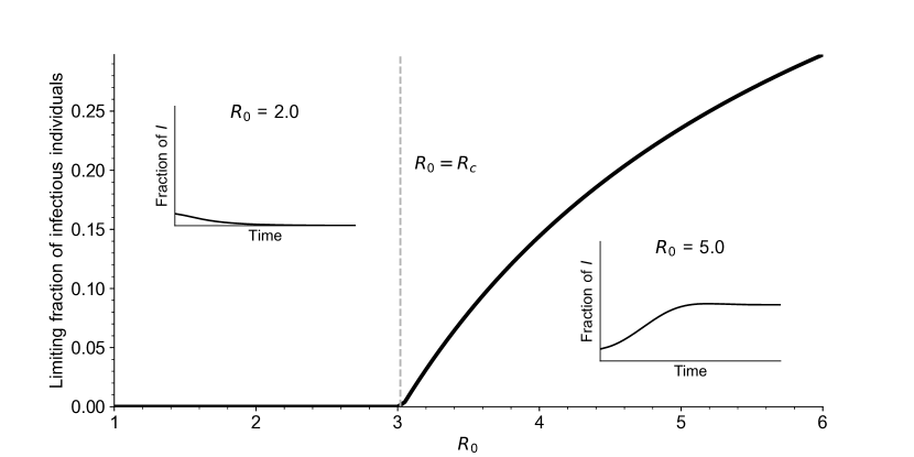
Figure 3: Bifurcation diagram for equation (4). For each value of $R_{0}$, the value of $\int_{0}^{\infty}I(t,a)\mathrm{d}a$ is reported, for a large time $t=5000$. The simulations are initialized with a fraction $I_{0}=0.1$ of infectious individuals, all other parameter values are given in Table 1 (Section A.6). The dashed vertical grey line indicates the endemic threshold $R_{0}$ computed from (14), above which we expect to see existence of a stable endemic equilibrium. In the two insets $\int_{0}^{\infty}I(s,a)\mathrm{d}a$ is plotted as a function of time $s\leq t$ for $R_{0}=2$ and $R_{0}=5$.

Figure 4: Left: Solutions of the PDE (4) for three values of $R_{0}$ and $\theta_{\sigma}$. The parameters correspond to the grey dots on the right plot. All other parameters are given in Table 1 (Section A.6). Right: Bifurcation diagram of equation (4), as a function of $R_{0}$ and $\theta_{\sigma}$ (scale parameter, defined in Section A.6.1). Each point of the heatmap represents the value of $\int_{0}^{\infty}I(t,a)\mathrm{d}a$ for a large time $t=300$. The grey curve is the endemic threshold $R_{c}$ in (14) as a function of $\theta_{\sigma}$.

In Figure 3 and Figure 4 we draw the bifurcation diagram of our system, as well as some typical trajectories of the fraction of infected individuals in our model. A first observation is that, on the simulation displayed in Figure 3 and in all simulations carried out by the authors, the model exhibits a simple asymptotic behavior. The epidemic either dies out, in the sense that the fraction of infected individuals goes to $0$, or survives in which case the fraction of infected individuals converges to a positive value. Moreover, the region of parameters for which the epidemic survives coincides with the region of parameters for which $R_{0}>R_{c}$, that is, for which we predict the existence of an endemic equilibrium.

Overall, this suggests that the asymptotic behavior of our model is very similar to that of the more usual systems of ordinary differential equations of the SIRS type: when an endemic equilibrium exists, it is globally asymptotically stable, otherwise the disease-free equilibrium is globally asymptotically stable. When $R_{0}$ crosses the threshold $R_{c}$, we observe an exchange of stability of the two equilibria, similar to a transcritical bifurcation.

Let us make a final remark. The solution to the PDE (4) has a probabilistic interpretation as the age distribution of the solution to the McKean–Vlasov equation (3). In this probabilistic setting, existence of an endemic equilibrium translates into existence of a stationary age distribution, and proving the asymptotic stability of this equilibrium amounts to proving convergence of the age distribution towards the stationary distribution. This connexion could provide a way to study the stability of endemic equilibria analytically. We refer to models using piecewise deterministic Markov processes with age dependence (e.g., Bouguet (2015); Fournier and Löcherbach (2016)).

4 Impact of the vaccination policy on endemicity

In the light of the results of the previous section, the long-term behavior of the epidemic depends mostly on three parameters, namely $R_{0}$, $\mathcal{L}_{\sigma}$ and $\mathcal{L}_{V}$ (the distributions of $\sigma$ and $T_{V}$). In this section, we discuss the impact that policy-making can have on the control of the epidemic through changing these parameters.

Policy-making does not impact these three parameters in the same way. The basic reproduction number $R_{0}$ can be lowered by reducing the contact rate in the population, but is not dependent on the way vaccines are administrated. We will consider it as fixed since we are mostly interested in studying the impact of vaccination rather than changes in the contact rate. Similarly, we think of $\sigma$ as reflecting the protection against reinfection provided by the host immunity. The waning of this protection is therefore dictated by the biological features of the disease and of the host immunity, which cannot be influenced by policy-making. (We do neglect the fact that part of the variation of the susceptibility might come from behavioral changes that could be affected by policy.) We also consider the law $\mathcal{L}_{\sigma}$ of $\sigma$ as being fixed. Finally, we think of $T_{V}$ as resulting from the vaccination strategy being applied. Typically, the law of $T_{V}$ depends on the number of doses administrated, on the instructions given to the general population on when and how often to get vaccinated, and on how these instructions are being followed. The law of $T_{V}$ has a complicated effect on the outcome of the disease, which depends strongly on the distribution of $\sigma$ and that we aim to study.

In the rest of this work, we will use $R_{c}$ (or $\Sigma$) as an indicator of the efficiency of the vaccination policy, and try to see what distribution $\mathcal{L}_{V}$ of $T_{V}$ might achieve a higher $R_{c}$ (or equivalently a lower $\Sigma$).

4.1 The cost of a vaccination policy

Intuitively, vaccinating the population more often on average should result in a higher protection against transmissions, but comes at a higher cost (of producing the vaccines and deploying them for instance). We will quantify this cost in order to compare the efficiency of a vaccination strategy (that is, of a distribution of $T_{V})$ relative to its cost, and not only in absolute terms.

A natural measure of the cost of a vaccination policy is the per capita per unit of time number of vaccine doses that are injected. In our model, the number of doses injected between time $t$ and $t+\mathrm{d}t$ is

$$\int_{0}^{\infty}S(t,a)\mu_{V}(a)\mathrm{d}a\cdot\mathrm{d}t.$$

If the population is at the disease-free equilibrium (8), a simple computation shows that the number of doses administrated per unit of time is

$$\int_{0}^{\infty}S(a)\mu_{V}(a)\mathrm{d}a=\frac{1}{\mathbb{E}[T_{V}]}.$$

We argue that, as long as the incidence and prevalence of the disease is low, the number of vaccines doses used per unit of time at the endemic equilibrium can also be approximated by $1/\mathbb{E}[T_{V}]$.

Let us consider that the population is at an endemic equilibrium, and that the incidence is negligible, that is, that $I(0)\ll 1$. Using (9) and the latter assumption on the incidence,

$$\int_{0}^{\infty}I(a)\mathrm{d}a=I(0)\mathbb{E}[T_{I}]\ll 1$$

so that the prevalence of the disease should also be low. From (10) and using $I(0)\ll 1$ we compute that the number of doses injected per unit of time at the endemic equilibrium is approximated by

$$\int_{0}^{\infty}S(0)\mu_{V}(a)\exp\left(-\int_{0}^{a}\mu_{V}(u)\mathrm{d}u\right)\mathbb{E}\left[e^{-I(0)R_{0}\int_{0}^{a}\sigma(u)\mathrm{d}u}\right]\mathrm{d}a\approx S(0).$$

Using that the prevalence is negligible, we further deduce from

$$1=\int_{0}^{\infty}S(a)\mathrm{d}a+\int_{0}^{\infty}I(a)\mathrm{d}a\approx\int_{0}^{\infty}S(0)\exp\left(-\int_{0}^{a}\mu_{V}(u)\mathrm{d}u\right)\mathrm{d}a=S(0)\mathbb{E}[T_{V}]$$

that the number of doses is approximated by $S(0)\approx 1/\mathbb{E}[T_{V}]$.

Overall, based on this heuristic computation we will use $1/\mathbb{E}[T_{V}]$ as an indicator of the cost of a vaccination strategy $T_{V}$.

4.2 Impact of the vaccination strategy

We now study the effect of modifying the distribution of $T_{V}$ on the value of $\Sigma$ defined in (15). By using Fubini’s theorem, let us first re-write the expression for $\Sigma$ as

$$\Sigma=\frac{\mathbb{E}\big{[}\int_{0}^{T_{V}}\sigma(a)\mathrm{d}a\big{]}}{\mathbb{E}[T_{V}]}=\frac{\mathbb{E}[\Phi(T_{V})]}{\mathbb{E}[T_{V}]}$$

where the deterministic function $\Phi$ is defined as

$$\forall t\geq 0,\quad\Phi(t)=\mathbb{E}\Big{[}\int_{0}^{t}\sigma(a)\mathrm{d}a\Big{]}=\int_{0}^{t}\mathbb{E}[\sigma(a)]\mathrm{d}a.$$

Optimal strategy for a fixed cost.

We assume that only a fixed number of doses can be administrated per unit of time in the population, say $1/m$, so that we restrict our attention to random variables $T_{V}$ verifying $\mathbb{E}[T_{V}]=m$. What distribution of $T_{V}$ then achieves the smallest value of $\Sigma$? In other words, given a fixed daily number of doses available, how are these doses best distributed to achieve the highest average immunity level in the population?

It turns out that this question is easily answered analytically. Since $a\mapsto\sigma(a)$ is a.s. nondecreasing, the function $a\mapsto\Phi(a)$ is convex. Therefore, applying Jensen’s inequality we obtain that

$$\Sigma=\frac{\mathbb{E}[\Phi(T_{V})]}{\mathbb{E}[T_{V}]}\geq\frac{\Phi(m)}{m}$$

where we recall that we have assumed that $\mathbb{E}[T_{V}]=m$. We see that the right-hand side of the previous inequality, $\Phi(m)/m$, is the susceptibility at the disease-free equilibrium when $T_{V}=m$ almost surely. It corresponds to an idealized situation where each individual gets vaccinated every $m$ unit of time, exactly. Therefore, given a vaccination strategy $T_{V}$, a better strategy that uses the same number of doses is always to let each individual receive vaccines at evenly spaced moments.

The optimal allocation strategy with $\mathbb{E}[T_{V}]=m$ is achieved by letting $T_{V}=m$ a.s., that is, by letting $T_{V}$ follow the distribution with the smallest dispersion. More generally, we argue that a distribution of $T_{V}$ which is less dispersed performs better at preventing an endemic state. Intuitively, if $T_{1}$ is less dispersed than $T_{2}$ and both have the same mean, $T_{2}$ puts more mass towards larger values. Then, loosely speaking $\mathbb{E}[\Phi(T_{2})]$ should be larger, since it is the integral of a convex function and that the mass a measure puts on large values typically contributes a lot to the integral of that function. Being more rigorous, one common way to formalize the notion of dispersal is to use the notion of convex ordering (Shaked and Shanthikumar, 2007, Chapter 3). A random variable $T_{1}$ is smaller in convex ordering then another random variable $T_{2}$ if

$$\forall\phi\text{ convex},\quad\mathbb{E}[\phi(T_{1})]\leq\mathbb{E}[\phi(T_{2})]$$

which we write as $T_{1}\preceq T_{2}$. Being larger in convex ordering is a common indicator of larger dispersion. Trivially, if $T_{1}\preceq T_{2}$ and $\Sigma_{1}$ and $\Sigma_{2}$ are the respective stationary susceptibilities, we have that $\Sigma_{1}\leq\Sigma_{2}$. Overall, this indicates that larger variability in the vaccination times perform worse at preventing the spread of the disease.

Effect of increasing the vaccination effort.

We now consider the effect of varying the mean of $\mathbb{E}[T_{V}]$, which can be interpreted as varying the number of vaccine doses administrated in the population. Intuitively, one would expect that reducing $\mathbb{E}[T_{V}]$ (that is, vaccinating more) also reduces the stationary susceptibility $\Sigma$. However, it is not hard to come up with counter-examples where this is not the case, and no conclusion can be drawn in general.

Nonetheless, it is a reasonable assumption to suppose that increasing the number of vaccines administrated will not completely change the shape of the distribution of $T_{V}$, but rather modify it in a continuous way. One way to model this is to consider a variable $m\geq 0$ representing (inverse of) the vaccination effort, and to assume that when at vaccination effort $m$, the vaccination period distribution is given by $mT_{V}$, for a fixed $T_{V}$. This way, increasing the number of vaccines only changes the scale of the distribution. Clearly, since $\Phi$ is convex, the function

$$m\mapsto\frac{\mathbb{E}[\Phi(mT_{V})]}{\mathbb{E}[mT_{V}]}$$

is increasing. We do recover the expected and intuitive behaviour: as $m$ increases, less vaccines are administrated, and $\Sigma$ increases, that is, the population becomes more susceptible to the disease.

5 Public health applications

As an application of our model, we now study in more details two specific situations. In the first situation, we assume that a fraction of the population does not get vaccinated. This could reflect among other examples vaccine hesitancy, impossibility to receive a vaccine, or unequal access to the vaccination. We want to understand the impact at the population level of having such a subpopulation that is not vaccinated, and to derive an expression for the minimal fraction of the population that needs to be vaccinated to prevent endemicity.

In the second situation, we consider that the population is divided into two groups, which can represent two distinct physical locations (cities, countries), or two groups in a heterogeneous population. We assume that a fixed number of vaccine doses can be administrated per unit of time, due to resource limitation, such as limited vaccine production or deployment. We investigate the impact of an uneven allocation of these doses between the two groups.

In both situations the population is no longer homogeneous, in the sense that it is made of several groups, with a different vaccination policy enforced in each group. We start by making a straightforward extension of our model to such a heterogeneous population in Section 5.1. We will derive briefly in Section 5.2 a corresponding law of large number and criterion for the existence of an endemic equilibrium, similar to that for the homogeneous model. Finally we study our two situations in Section 5.3.

5.1 Modeling vaccination heterogeneity

We present in this section the general case of a population of size $N$ divided into $L$ fixed subgroups according to the vaccination policy in each subgroup (within each subgroup, the vaccination times of each individual have the same distribution). We allow the contact rates to vary between different subgroups according to some contact matrix. We assume that the infectiousness and susceptibility curves do not depend on the subgroup, they are the same for the whole population. Let us give a more precise definition of the dynamics, and of the parameters of this extension.

Description.

Suppose that each of the $N$ individuals in the population now belongs to one of $L$ groups, labeled by $\ell\in\{1,\dots,L\}$, and that this group remains at all time. The number of individuals in group $\ell$ is denoted by $N_{\ell}$, and we assume that $N_{\ell}/N\to p_{\ell}\in(0,1)$ as $N\to\infty$. An individual is now identified by a pair $(\ell,i)$, $\ell$ being its group and $i\leq N_{\ell}$ its label within group $\ell$. We will denote its infectiousness and susceptibility at time $t$ as $\lambda^{N}_{\ell,i}(t)$ and $\sigma^{N}_{\ell,i}(t)$ respectively.

Individuals follow the same dynamics as described in Section 2.1, but the group of an individual affects the rate at which it gets vaccinated. In particular upon entry in the $I$ state an individual samples an infectious period $T_{I}$ and an infectiousness $\lambda$ according to the same distribution $\mathcal{L}_{\lambda}$ as in the homogeneous model, regardless of its group. Upon entry in the $S$ state, the susceptibility $\sigma$ of any individual is also sampled according to the same common distribution $\mathcal{L}_{\sigma}$ which does not depend on the group. However the time until the next vaccination of an individual in group $\ell$ is now given by a random variable denoted by $T_{\ell}$ whose distribution depends on the group. (Note that we have dropped the $V$ subscript to ease the notation.)

Moreover, we assume that contacts in the population are heterogeneous, which we encode as a symmetric matrix $\Gamma=(\gamma_{\ell,\ell^{\prime}})$, where $\gamma_{\ell,\ell^{\prime}}=\gamma_{\ell^{\prime},\ell}\geq 0$ gives the contact intensity between an individual of group $\ell$ and one of group $\ell^{\prime}$. We assume that this contact matrix does not depend on the size of the population $N$. Note that $\gamma_{\ell,\ell^{\prime}}$ corresponds to a contact rate per pair of individuals, so that the overall contact rate between group $\ell$ and group $\ell^{\prime}$ is $\gamma_{\ell,\ell^{\prime}}N_{\ell}N_{\ell^{\prime}}$. The rate at which individual $(\ell,i)$ gets infected at time $t$ is

$$\sigma^{N}_{\ell,i}(t)\cdot\sum_{\ell^{\prime}=1}^{L}\gamma_{\ell^{\prime},\ell}\Lambda^{N}_{\ell^{\prime}}(t)$$

where

$$\Lambda^{N}_{\ell}(t)=\frac{1}{N}\sum_{i^{\prime}=1}^{N_{\ell}}\lambda^{N}_{\ell,i^{\prime}}(t).$$

In words, each individual $(\ell^{\prime},i^{\prime})$ makes an infectious contact with $(\ell,i)$ at rate $\gamma_{\ell^{\prime},\ell}\lambda^{N}_{\ell^{\prime},i^{\prime}}(t)/N$, and such an infectious contact at time $t$ yields an infection with probability $\sigma^{N}_{\ell,i}(t)$.

This model could be easily made more general by allowing the distribution of the infectiousness and susceptibility $\mathcal{L}_{\lambda}$ and $\mathcal{L}_{\sigma}$ to depend on the group. This could represent various vulnerability to the disease for instance.

Large population size limit.

As in the homogeneous model, we can derive a law of large numbers limit for the age and state structure of the epidemic. Let the empirical measure of ages of $I$ and $S$ individuals in group $\ell$ be denoted respectively as

$$\nu_{I,\ell}^{N}(t)=\frac{1}{N}\sum_{\begin{subarray}{c}i=1,\dots,N_{\ell}\\ C^{N}_{\ell,i}(t)=I\end{subarray}}\delta_{A^{N}_{\ell,i}(t)},\quad\nu_{S,\ell}^{N}(t)=\frac{1}{N}\sum_{\begin{subarray}{c}i=1,\dots,N_{\ell}\\ C^{N}_{\ell,i}(t)=S\end{subarray}}\delta_{A^{N}_{\ell,i}(t)}$$

If the initial age structures converge, the latter empirical measures should converge respectively, as $N\to\infty$, to the solution $(I_{\ell}(t,a);\,a\geq 0)$ and $(S_{\ell}(t,a);\,a\geq 0)$ of the following multidimensional version of equation (4),

$$\begin{split}\partial_{t}I_{\ell}(t,a)+\partial_{a}I_{\ell}(t,a)&=-\mu_{I}(a)I_{\ell}(t,a)\\ \partial_{t}S_{\ell}(t,a)+\partial_{a}S_{\ell}(t,a)&=-\mu_{V,\ell}(a)S_{\ell}(t,a)-\sum_{\ell^{\prime}=1}^{L}\gamma_{\ell^{\prime},\ell}\Lambda_{\ell^{\prime}}(t)\cdot\mathbb{E}_{t,a;\ell}[\sigma(a)]S_{\ell}(t,a)\\ I_{\ell}(t,0)&=\sum_{\ell^{\prime}=1}^{L}\gamma_{\ell^{\prime},\ell}\Lambda_{\ell^{\prime}}(t)\cdot\int_{0}^{\infty}\mathbb{E}_{t,a;\ell}[\sigma(a)]S_{\ell}(t,a)\mathrm{d}a\\ S_{\ell}(t,0)&=\int_{0}^{\infty}\mu_{V,\ell}(a)S_{\ell}(t,a)\mathrm{d}a+\int_{0}^{\infty}\mu_{I}(a)I_{\ell}(t,a)\mathrm{d}a.\end{split}$$ (17)

The initial condition of this system of PDE is a straightforward extension of that in equation (4) and we do not write it down explicitly. Nevertheless note that the initial condition should fulfill that

$$\forall\ell\leq L,\quad\int_{0}^{\infty}I_{\ell}(0,a)+S_{\ell}(0,a)\mathrm{d}a=p_{\ell},$$

where $p_{\ell}=\lim_{N\to+\infty}{N_{\ell}}/{N}.$

In the previous equation, $\mu_{V,\ell}(a)$ denotes the hazard rate of the vaccination time $T_{\ell}$ in group $\ell$, and we define

$$\Lambda_{\ell}(t)=\int_{0}^{\infty}I_{\ell}(t,a)\mathbb{E}[\lambda(a)\mid T_{I}>a]\mathrm{d}a$$

and

$$\mathbb{E}_{t,a;\ell}[\sigma(a)]=\mathbb{E}\Big{[}\sigma(a)\exp\Big{(}-\int_{0}^{a}\sum_{\ell^{\prime}=1}^{L}\gamma_{\ell^{\prime},\ell}\Lambda_{\ell^{\prime}}(t-a+u)\sigma(u)\mathrm{d}u\Big{)}\Big{]}\\ \Big{/}\>\mathbb{E}\Big{[}\exp\Big{(}-\int_{0}^{a}\sum_{\ell^{\prime}=1}^{L}\gamma_{\ell^{\prime},\ell}\Lambda_{\ell^{\prime}}(t-a+u)\sigma(u)\mathrm{d}u\Big{)}\Big{]}.$$

All other terms have been defined in Section 2.3.

5.2 Endemicity criterion for heterogeneous vaccination

Again, we study the equilibria of (17) to derive a criterion for the existence of an endemic equilibrium. We look for solutions of (17) of the form

$$\forall t,a\geq 0,\>\forall\ell\in\{1,\dots,L\},\quad I_{\ell}(t,a)=I_{\ell}(a),\quad S_{\ell}(t,a)=S_{\ell}(a).$$

We will assume from now on that the matrix $\Gamma$ is irreducible. In this case, it is not hard to see that there are only two possible types of equilibria: either the disease is absent in each groups ($I_{\ell}\equiv 0$ for all $\ell\in\{1,\dots,L\}$) or it is endemic in each group ($I_{\ell}>0$ for all $\ell\in\{1,\dots,L\}$). Naturally, we will refer to the former situation as the disease-free equilibrium, and to the latter one as the endemic equilibrium.

Disease-free equilibrium.

As in the homogeneous case, in the absence of infected individuals, each group gets vaccinated according to a different renewal process. It is easy to check that the only equilibrium of (17) with $I_{\ell}(a)\equiv 0$ for all $\ell\geq 1$ is given by

$$\forall a\geq 0,\>\forall\ell\in\{1,\dots,L\},\quad S_{\ell}(a)=\frac{p_{\ell}}{\mathbb{E}[T_{\ell}]}\exp\Big{(}-\int_{0}^{a}\mu_{V,\ell}(u)\mathrm{d}u\Big{)}.$$

Endemic equilibrium.

In principle, we could use the same arguments as in the homogeneous case and find a set of $L$ coupled equation similar to (12) that characterize the existence of stationary points of (17). However solving this equation would prove to be an even more difficult task, since we are now dealing with a multi-dimensional equation. We choose not to go in this direction and prefer to start from the connection between the endemicity criterion in the homogeneous case and the survival of a well-chosen branching process.

Suppose that a single infected individual of group $\ell$ is introduced in a population at the disease-free equilibrium. Over its entire infectious period, this individual makes on average $p_{\ell^{\prime}}\gamma_{\ell,\ell^{\prime}}R_{0}$ infectious contacts with individuals of type $\ell^{\prime}$. An individual of group $\ell^{\prime}$ targeted by an infectious contact has a random susceptibility. The expectation of this random variable is the mean susceptibility at the disease-free equilibrium of group $\ell^{\prime}$, that is,

$$\Sigma_{\ell^{\prime}}\coloneqq\frac{1}{p_{\ell^{\prime}}}\int_{0}^{\infty}S_{\ell^{\prime}}(a)\mathbb{E}[\sigma(a)]\mathrm{d}a=\frac{\mathbb{E}\big{[}\int_{0}^{T_{\ell^{\prime}}}\sigma(a)\mathrm{d}a\big{]}}{\mathbb{E}[T_{\ell^{\prime}}]}.$$

Therefore, an infected individual of group $\ell$ produces on average $R_{0}m_{\ell,\ell^{\prime}}$ secondary infections in group $\ell^{\prime}$, with

$$m_{\ell,\ell^{\prime}}:=p_{\ell^{\prime}}\gamma_{\ell,\ell^{\prime}}\Sigma_{\ell^{\prime}}.$$ (18)

We introduce the matrix

$${M:=(m_{\ell,\ell^{\prime}})_{1\leq\ell,\ell^{\prime}\leq L}}.$$

According to the previous discussion, the epidemic generated by a single infected individual can be thought of as a multi-type branching process with mean offspring matrix $R_{0}M$. The type of an individual in the branching process corresponds to the group to which it belongs. It is now a classical result from the theory of branching processes that, under our mild condition that the contact matrix $\Gamma$ is irreducible, the latter branching process can survive with positive probability if and only if the leading eigenvalue of its mean offspring matrix $R_{0}M$ is larger than $1$, that is, if and only if $R_{0}>R_{c}$, where $1/R_{c}$ is the leading eigenvalue of the matrix $M$ (Athreya and Ney, 1971, Chapter V). (Note that this definition agrees with (14) when there is a single group, $L=1$, so that we use the same notation.) This is again reminiscent of the next-generation matrix techniques of Diekmann et al. (1990, 2010).

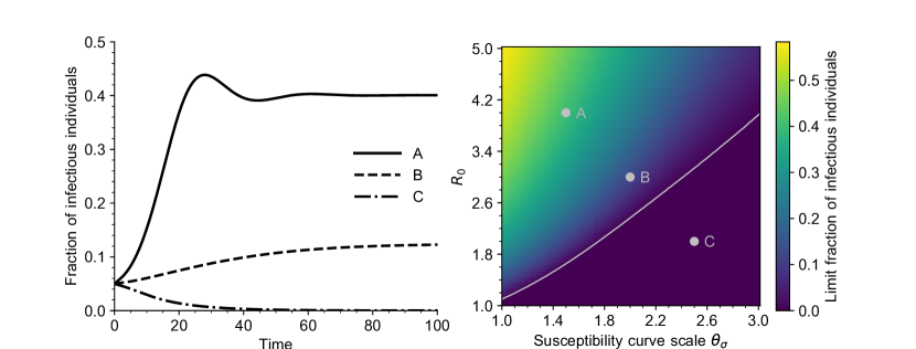
Figure 5: Left: Solutions of the PDE (4) for three values of $R_{0}$ and $\theta_{\sigma}$. The parameters correspond to the grey dots on the right plot. All other parameters are given in Table 1 (Section A.6). Right: Bifurcation diagram of equation (17), as a function of $R_{0}$ and $\theta_{\sigma}$ (scale parameter, defined in Section A.6.1). The population is made of three subpopulations with contact matrix and vaccination parameters given in Table 2. Each point of the heatmap represents the value of the total fraction of infectious individuals $\int_{0}^{\infty}I_{1}(t,a)+I_{2}(t,a)+I_{3}(t,a)\mathrm{d}a$ for a large time $t=300$. The grey curve is the endemic threshold $R_{c}$ in (14) as a function of $\theta_{\sigma}$.

Asymptotic behavior.

As in the case of homogeneous contacts, we are ultimately interested in assessing the effect of the parameters of the model on the persistence of the disease in the population for a long time. The criterion that we have derived above for the existence of an endemic equilibrium is heuristic, and does not guarantee that the state of the population converges to that endemic equilibrium when it exists.

Again, we study these questions numerically, by considering the bifurcation diagram of our model in Figure 5, in the case of three subpopulations. The trajectory of the total fraction of infected individuals among all groups is plotted for a sample of typical trajectories. As in the homogeneous case, the asymptotic behavior of the model is simple, and it seems to converge to a limit. In this limit, depending on the parameters, the epidemic is either extinct, or has reached an endemic equilibrium. Again, we see a good agreement between our theoretical prediction for the existence of an endemic equilibrium ($R_{0}>R_{c}$) and the parameter region where the epidemic does not go extinct. This also validates that our heuristic, based on the survival probability of a certain multi-type, seems to give the right criterion for the existence of an endemic equilibrium.

5.3 Two public health applications

The contact matrix $\Gamma$ introduces many new parameters to the model. We now restrict our attention to the case $L=2$ of two subpopulations which remains tractable. We further reduce the number of parameters by assuming that all groups have the same activity level. That is, we assume that individuals each group makes on average the same total number of contacts. Without loss of generality, we can assume that this average number of contacts is $1$, which leads to the constraint that

$$p_{1}\gamma_{1,1}+p_{2}\gamma_{1,2}=1,\qquad p_{1}\gamma_{1,2}+p_{2}\gamma_{2,2}=1.$$ (19)

In the case of a general number of groups $L$ this condition would read

$$\forall\ell\in\{1,\dots,L\},\quad\sum_{\ell^{\prime}=1}^{L}p_{\ell^{\prime}}\gamma_{\ell,\ell^{\prime}}=1.$$

For $L=2$, under assumption (19) and the additional constraint that contacts are symmetric, all contact matrices can be parametrized as

$$\Gamma=\begin{pmatrix}\frac{1}{p_{1}}(1-p_{2}\alpha)&\alpha\\ \alpha&\frac{1}{p_{2}}(1-p_{1}\alpha)\end{pmatrix}$$ (20)

for some $\alpha\in\left[0,\min\left(\frac{1}{p_{1}},\frac{1}{p_{2}}\right)\right]$. The remaining degree of freedom $\alpha$, which we will refer to as the contact parameter, tunes the assortativity of the contacts:

• for $\alpha\in[0,1)$ the population is assortative and individuals make more contacts within their own group (for $\alpha=0$ the populations would be disconnected);

• for $\alpha=1$ the population is well-mixed and contacts are homogeneous;

• for $\alpha\in\left(1,\min\left(\frac{1}{p_{1}},\frac{1}{p_{2}}\right)\right]$ the population is dissortative and individuals make more contacts outside of their groups.

Under this parametrization, the endemic threshold is given by the inverse of the leading eigenvalue of the matrix

$$M=\begin{pmatrix}(1-p_{2}\alpha)\Sigma_{1}&p_{2}\alpha\Sigma_{2}\\ p_{1}\alpha\Sigma_{1}&(1-p_{1}\alpha)\Sigma_{2}\end{pmatrix}.$$

The leading eigenvalue of this matrix corresponds to the largest root of the equation

$$\rho^{2}-((1-p_{1}\alpha)\Sigma_{2}+(1-p_{2}\alpha)\Sigma_{1})\rho+(1-\alpha)\Sigma_{1}\Sigma_{2}$$

which is written down explicitly in (A.5) in Section A.5.

General results on two groups

Before moving to our specific applications, let us make two general observations. First, we can prove (see Proposition 6 in Section A.5) that the leading eigenvalue of $M$ is decreasing in the contact parameter $\alpha$. It means that the endemicity threshold $R_{c}$ is maximal for dissortative populations, when the other parameters are fixed. We cannot deduce optimal vaccine strategies from this fact, because public health policies have little influence on this parameter. However, this result is interesting in itself and will be useful in the problem of optimal vaccine allocation. Second, if vaccine doses are allocated in the same way for each the two groups we have $\Sigma_{1}=\Sigma_{2}\eqqcolon\Sigma$. The matrix $M$ is easily seen to be a multiple of a stochastic matrix, with leading eigenvalue $\Sigma$, and the criterion for the existence of an endemic equilibrium simplifies to that for an homogeneous population, namely $R_{0}\Sigma>1$. Therefore, when vaccine doses are allocated fairly among the population and groups have the same activity level (equation (19) holds), the population structure does not impact the existence of an endemic equilibrium. A similar claim holds more generally for any number of groups $L$.

Effect of vaccine hesitancy

We model partial vaccination of the population by assuming that individuals from group $1$ get vaccinated whereas individuals from group $2$ do not. Let $\Sigma\coloneqq\Sigma_{1}$ be the mean susceptibility at the disease-free equilibrium within group $1$. Let us assume that almost surely $\sigma(a)\to 1$ as $a\to\infty$, so that individuals immunity vanishes completely after a long-enough time. Since group $2$ does not get vaccinated, the mean susceptibility in this group is set to be $\Sigma_{2}=1$.

We further assume for simplicity that the population is well-mixed $\alpha=1$, so that the mean offspring matrix is

$$M=\begin{pmatrix}p_{1}\Sigma_{1}&p_{2}\\ p_{1}\Sigma_{1}&p_{2}\end{pmatrix}$$

and we can readily check that its leading eigenvalue is

$$R_{c}=\frac{1}{p_{1}\Sigma+p_{2}}=\frac{1}{1-(1-\Sigma)p_{1}}.$$

Define a critical fraction $p_{c}$ as

$$p_{c}\coloneqq\frac{1-1/R_{0}}{1-\Sigma}.$$

Then $p_{c}$ gives the critical fraction of the population that needs to be vaccinated recurrently to prevent an endemic equilibrium, that is

$$R_{0}\leq R_{c}\iff p_{1}\geq p_{c}.$$

There is an interesting correspondence between this formula and the well-known formula that gives the critical vaccine coverage to prevent an epidemic (Anderson and May, 1982; Anderson et al., 2020). If a vaccine has an efficacy $E\in[0,1]$ (that is it provides a sterilizing immunity with probability $E$) then the critical fraction of the population that needs to be vaccinated to prevent an epidemic is

$$p^{\prime}_{c}=\frac{1-1/R_{0}}{E}.$$

In our model, the efficiency of the vaccine policy is quantified by $1-\Sigma$ which corresponds to the fraction of infections that are blocked at the stationary disease-free equilibrium if all individuals get vaccinated.

Optimal vaccine allocation between two groups

Consider a second situation where a fixed number of vaccine doses per unit of time is available, and these doses need to be allocated between two groups of individuals, which do not necessarily make homogeneous contacts. (The contact heterogeneity accounts for the fact that the groups may be two physically distinct locations: cities, countries, regions.) We model this situation in the following way.

Let $T_{1}$ and $T_{2}$ be the vaccination times in each group with expectations $m_{1}=\mathbb{E}[T_{1}]$ and $m_{2}=\mathbb{E}[T_{2}]$, and let $1/m$ be the per unit of time number of doses that can be allocated in the total population. Since the number of doses injected in group $\ell$ is $p_{\ell}/\mathbb{E}[T_{\ell}]$, the fact that the total number of doses injected in the population is $1/m$ adds the constraint that

$$\frac{p_{1}}{\mathbb{E}[T_{1}]}+\frac{p_{2}}{\mathbb{E}[T_{2}]}=\frac{p_{1}}{m_{1}}+\frac{p_{2}}{m_{2}}=\frac{1}{m}.$$ (21)

The set of all pairs $(m_{1},m_{2})$ verifying (21) for a given $m$ can now be parametrized by a single parameter $\beta$ as

$$\forall\beta\in\left[-\frac{1}{p_{2}},\frac{1}{p_{1}}\right],\quad\frac{1}{m_{1}(\beta)}=\frac{1}{m}+\frac{p_{2}}{m}\beta,\quad\frac{1}{m_{2}(\beta)}=\frac{1}{m}-\frac{p_{1}}{m}\beta.$$

Under this parametrization, we can interpret $\beta$ as assessing the fairness of the allocation in the sense that

• when $\beta=0$, all doses are allocated evenly across the two groups;

• when $\beta>0$ population 1 is favored and, if $\beta=\frac{1}{p_{1}}$ all the doses are allocated to population $1$;

• when $\beta<0$ population 2 is favored and, if $\beta=-\frac{1}{p_{2}}$, all the doses are allocated to population $2$.

We now choose a family of random variables $(T_{1}(\beta),T_{2}(\beta))$ such that $\mathbb{E}[T_{\ell}(\beta)]=m_{\ell}(\beta)$, which represent a possible allocation of the doses with fairness parameter $\beta$. We choose a natural family of such random variables, defined as

$$T_{1}(\beta)=\frac{1}{1+\beta p_{2}}T,\qquad T_{2}(\beta)=\frac{1}{1-\beta p_{1}}T$$ (22)

where $T$ is a common random variable with $\mathbb{E}[T]=m$.

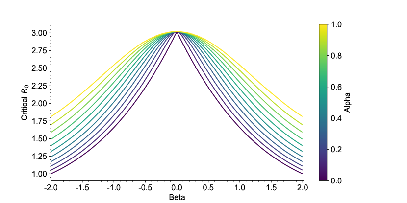
Figure 6: Behavior of $R_{c}$ as a function of the fairness parameter $\beta$, for different values of $\alpha$. The random variable $T$ in (22) has a Gamma distribution with shape and scale parameters given by $\kappa_{V}$ and $\theta_{V}$ respectively, as in Table 1 (Section A.6). The population is assumed to be made of two groups of the same size, $p_{1}=p_{2}=\tfrac{1}{2}$. All other parameters are given in Table 1 (Section A.6).

For this specific choice of $(T_{1}(\beta),T_{2}(\beta))$ we can prove that when the population is assortative ($\alpha\leq 1$) the strategy that performs the best is the fair strategy ($\beta=0$).

Proposition 4.

Let $(T_{1}(\beta),T_{2}(\beta))$ be as in (22) and let $R_{c}(\beta)$ be the corresponding endemic threshold computed as the reciprocal of the largest eigenvalue of (18). Then for any fixed number of doses $m>0$ and any $\alpha\in[0,1]$, $\beta\mapsto R_{c}(\beta)$ is maximal at $\beta=0$.

This result is proved in Section A.5, and illustrated in Figure 6. Therefore, for our example, allocating a larger share of the vaccines to a specific subpopulation results in an additional cost to the overall population, since the disease can more easily reach an endemic state and persist.

6 Summary and discussion

Summary.

In this work we have proposed an individual-based model to study the effect of recurrent vaccination on the establishment of an endemic equilibrium, in a population with waning immunity. Our model incorporates memory effects both for the transmission rate during an infection and for the subsequent immunity, and takes into account the stochasticity at the individual level for these two processes. By deriving the large population size limit of the model and analysing its equilibria, we have obtained a simple criterion for the existence of an endemic equilibrium. This criterion depends jointly on the shape of the rate of immunity loss and on the distribution of the time between two booster doses. In other words, in the context of recurrent vaccination and waning immunity, what drives the result of a vaccination-policy is a combination of the efficiency of the vaccine itself at blocking transmissions, and of the way in which booster doses are distributed in the population. The expression we obtain relates directly to the average immunity level maintained by vaccinating recurrently the population, which is a relation that we expect to hold for a broad class of models with similar characteristics.

One general public health conclusion that we can draw from our work is that, for the same average number of vaccine doses available, vaccination strategies where the time between booster shots are more evenly spaced (at the individual level) perform better at blocking transmissions. Intuitively, irregularly spread booster doses lead to some longer time intervals without vaccination, and the resulting high susceptibility allows the disease to spread more efficiently. Deriving further conclusions from our model would require to add some restrictions on the distributions of $T_{V}$ and $\sigma$ that would reflect the characteristics of a particular disease and vaccine.

Finally, we have studied two specific situations in more details. First, we have computed an expression for the critical fraction of the population required to adhere to the vaccination policy to eradicate the disease. This expression is reminiscent of a well-known threshold for preventing an endemic state with an imperfect vaccine (Anderson and May, 1985). In the context of recurrent vaccination, the efficiency of the vaccine is replaced by the average susceptibility obtained by vaccinating individuals in the absence of disease. Second we have studied the consequences of uneven vaccine access in a population, and concluded that under reasonable assumptions fair vaccine allocation is the optimal strategy to prevent endemicity.

Model assumptions.

Our model is formulated in terms of infectiousness and susceptibility, which are two phenomenological quantities that result from the complex interaction between the pathogen and the host immune system. If this interaction were modeled explicitly as in many existing works on viral dynamics (Heffernan and Keeling, 2008, 2009; Goyal et al., 2020; Néant et al., 2021), infectiousness would relate to the viral load, and susceptibility to the level of immune cells or circulating antibodies. Since we have left the susceptibility and infectiousness be general random functions, our model should encompass many possible such host-pathogen models. There are two assumptions that we have made about $\lambda$ and $\sigma$ that could be easily relaxed mathematically, but would lead to a more complicated model. First, we assumed that the susceptibility curve following an infection is independent of the infectiousness curve during that infection. A typical situation where this assumption would fail is if a more severe infection leads both to a larger infectiousness and to a higher level of immunity (and thus a lower susceptibility). Second, we assumed that infection and vaccination lead to the same susceptibility in distribution. We expect a law of large number similar to Theorem 1 to hold if these assumptions are relaxed, with a similar criterion for the existence of an endemic equilibrium and mild modifications of the limit equations. However, our mathematical results rely crucially on the strong assumption that individuals (and thus their immune system) keep no memory of past infections or vaccinations: at each re-infection or vaccination, the subsequent infectiousness and susceptibility are sampled independently and according to the same law. In particular, the expression (15) for the herd immunity threshold follows from the fact that vaccinations form a renewal process, which is a consequence of this absence of memory from past vaccinations. Relaxing this assumption would require a completely different approach to our problem. Nonetheless, the key quantity in our model is the stationary susceptibility of a typical individual, obtained by letting an individual get vaccinated only for a long period of time. It might be the case that other models displaying a similar stationary behavior have the same qualitative properties as the one investigated here.

The persistence of a disease requires a continual replenishment of susceptible individuals to sustain the epidemic. In our model, this influx of susceptibility comes exclusively from waning immunity. Two other important causes for an increase in susceptibility that we have neglected are the birth of new individuals with no immunity, and the pathogen evolution to escape immunity. We expect that, as long as the population size is stable and newborns start being vaccinated rapidly, demographic effects (that we have neglected by considering a closed population) should not impact our conclusions to a large extent. The key quantity that controls the establishment of an endemic equilibrium in our model is the level of population immunity in the absence of disease, which should be mostly driven by vaccination if the typical time between two vaccine doses is small compared to the lifetime of individuals. Taking into account pathogen evolution is, however, a more challenging task that would require further investigation and modeling. Though, note that a model structured by time-since-recovery similar to the one we consider here has been proposed to study the increase in susceptibility due to antigenic drift in influenza strains (Pease, 1987).

Discussion.

In the second half of our work, we have used the endemic threshold $R_{c}$ to quantify the efficiency of a given vaccination policy. This criterion has the advantage of having a clear interpretation (in terms of the average level of susceptibility maintained by vaccination), of being easy to compute and of depending on only a few average quantities of the model: the basic reproduction number $R_{0}$, the expected susceptibility at a given time $\mathbb{E}[\sigma(a)]$ and the distribution of $T_{V}$. Another interesting indicator of the impact of a vaccination policy is the so-called endemic level, defined as the prevalence of the disease at the endemic equilibrium. Ultimately, it is this endemic level that public health measures try to control, to reduce the burden of the disease in the population. In our model, when an endemic equilibrium exists, the endemic level is given by $x\mathbb{E}[T_{I}]/R_{0}$, where $x$ solves $F_{\mathrm{e}}(x)=R_{0}$ as in Proposition 3. The endemic level is therefore only implicitly defined, which makes it more complicated to study both analytically and numerically. Investigating the impact of the vaccination policy on the endemic level, though important, would therefore require further work, and the conclusions reached in Section 5.3 could be altered by using this endemic level as a criterion for the efficiency of vaccination instead of the endemic threshold. Note that the question of the impact of the way immunity is waning on the endemic level has been the subject of a recent study (Khalifi and Britton, 2022).

The simplest epidemic models consider the spread of a disease in a population made of identical individuals, that are mixing homogeneously: individuals are equally susceptible to the disease, equally infectious once infected, and contacts are equally likely to occur between any pair of individuals in the population (Britton et al., 2019, Part I). Many works have studied the epidemiological consequences of relaxing these assumptions, to account for some of the heterogeneity which is observed in human populations (Britton et al., 2020; Brauer, 2008; Magal et al., 2016; Andreasen, 2011; David, 2018). In a similar way, we have added some heterogeneity to our model in Section 5 by assuming that the population is subdivided into a finite number of groups, and that contacts between groups are heterogeneous and that individuals in different groups get vaccinated according to different distributions of $T_{V}$. Since our focus is the impact of inhomogeneous vaccination on endemicity, we have assumed that all groups have the same activity level ($\Gamma\times\operatorname{Diag}(p)$ is a multiple of a stochastic matrix), and that they sample their infectiousness and susceptibility curves from the same distribution. Our model could be easily extended to allow the distribution of the infectiousness and susceptibility curves to depend on the group, and to general contact matrices $\Gamma$. Using the same heuristic arguments as in Section 5.2, we can derive a criterion for the existence of an endemic equilibrium in terms of the leading eigenvalue of a next-generation matrix similar to (18). However, although it is possible to derive such an expression, the joint effect of heterogeneous infectiousness, susceptibility, contact rates and vaccination rates on this criterion is extremely complex, and deriving any public health insight would require some further work.

It is interesting to compare our expression for the endemic threshold and that recently obtained in Forien et al. (2022), for a similar model but without vaccination. In Forien et al. (2022) it is shown that, in the absence of vaccination and using our notation, an endemic equilibrium exists if and only if

$$\mathbb{E}\Big{[}\frac{1}{R_{0}\sigma_{*}}\Big{]}<1$$ (23)

where $\sigma_{*}\coloneqq\lim_{a\to\infty}\sigma(a)$. The corresponding expression with vaccination that we have obtained is

$$\frac{\mathbb{E}[T_{V}]}{R_{0}\mathbb{E}\Big{[}\int_{0}^{T_{V}}\sigma(a)\mathrm{d}a\Big{]}}<1.$$ (24)

By letting $T_{V}\to\infty$, we expect that our model converges to the model considered in Forien et al. (2022) where no vaccination is taken into account. However, in the limit $T_{V}\to\infty$ our expression for the endemicity criterion becomes

$$\frac{1}{R_{0}\mathbb{E}[\sigma_{*}]}<1.$$ (25)

Note the surprising discrepancy between (23) and (25). This apparent contradiction can be resolved by noting that both expressions are specific cases of a more general formula. Let $\zeta(u)$ denote the susceptibility of a typical individual at age-of-infection $u$, that is, $u$ unit of time after its last infection, regardless of how many times it is vaccinated. Then mimicking the computations of Section 3.1 would suggest that the right threshold for the existence of an endemic equilibrium is given by

$$\mathbb{E}\Big{[}\lim_{a\to\infty}\frac{1}{R_{0}\frac{1}{a}\int_{0}^{a}\zeta(u)\mathrm{d}u}\Big{]}<1,$$ (26)

provided that the limit in the expectation exists. In the absence of vaccination, $\zeta(u)=\sigma(u)$ and we recover (23). In the presence of vaccination, letting $\sigma_{i}$ and $T_{i}$ be i.i.d., we have

$$\forall u\geq 0,\quad\zeta(u)=\sigma_{i}(u-(T_{1}+\dots+T_{i}))\mathbf{1}_{\{T_{1}+\dots+T_{i}\leq u<T_{1}+\dots+T_{i+1}\}}$$

and classical results on renewal process show that we recover (25). We believe that (26) should give the right threshold for the existence of an endemic equilibrium for a broader class of models.

Acknowledgements.1Acknowledgements.1AcknowledgementsAcknowledgementsAcknowledgements.1

Acknowledgements

The project was sponsored by Mathematics for Public Health (MfPH) initiative, in Canada, involving the Fields Institute, the Atlantic Association for Research in Mathematical Sciences (AARMS), the Centre de Recherches Mathématiques (CRM), and the Pacific Institute for Mathematical Sciences (PIMS). FFR acknowledges financial support from MfPH, the AXA Research Fund, the Glasstone Research Fellowship, and thanks Magdalen College Oxford for a senior Demyship. AC acknowledges Canada’s Natural Sciences and Engineering Research Council (NSERC) for funding (RGPIN-2019-07077) and the AXA Research Fund. HG acknowledges Canada’s Natural Sciences and Engineering Research Council (NSERC) for funding (RGPIN-2020-07239).

Appendix A Supplementary material

A.1 Formal construction of the model

In this section we provide a rigorous probabilistic construction of our stochastic model.

Initial condition [IC].

At time $t=0$, each individual is placed in the $I$ state with probability $I_{0}$, or in the $S$ state otherwise. We record the initial state of individual $i$ as a random variable $C_{i,0}$ such that

$$\mathbb{P}(C_{i,0}=I)=1-\mathbb{P}(C_{i,0}=S)=I_{0}.$$

Individuals are assigned an initial age $A_{i}(0)=-\tau_{i,0}$ such that the age of an $I$ individual is distributed as $h_{I}$ and that of an $S$ individual is distributed as $h_{S}$. Finally, if $i$ is in the $I$ state, it is assigned a initial infectiousness $\lambda_{i,0}$ which is distributed as the typical infectiousness $\lambda$ conditional on $T_{I}>-\tau_{i,0}$, so that the individual remains infectious at time $t=0$. If $i$ is in the $S$ state, it is assigned two independent variables: a susceptibility $\sigma_{i,0}$ distributed as the typical susceptibility $\sigma$ and an initial vaccination time distributed as $T_{V,i,0}$, conditional on $T_{V}>-\tau_{i,0}$. All these variables are assigned independently for different individuals.

Spread of the epidemic.

Consider, for each $i$, three independent i.i.d. sequences, $(\lambda_{i,k},T_{I,i,k};\,k\geq 1)$, $(\sigma_{i,k};\,k\geq 1)$, $(T_{V,i,k};\,k\geq 1)$ distributed as $\mathcal{L}_{\lambda}$, $\mathcal{L}_{\sigma}$ and $\mathcal{L}_{V}$. We also introduce an auxiliary sequence of independent exponential random variables $(E_{i,k};1\leq i\leq N,k\geq 1)$ with unit mean, independent of the previous sequences.

From these random variables and the initial condition, we will construct two sequences of random variables $(\tau_{i,k};\,1\leq i\leq N,k\geq 1)$ and $(C_{i,k};\,1\leq i\leq N,k\geq 1)$ that represent respectively the time at which $i$ experiences its $k$-th event (infection, recovery, or vaccination), and its state after this $k$-th event ($I$ or $S$). Assuming that these variables are constructed, the age $A_{i}(t)$, the state $C_{i}(t)$, the infectiousness $\lambda_{i}(t)$ and susceptibility $\sigma_{i}(t)$ of individual $i$ at time $t$ are then simply given by

$$A_{i}(t) =t-\tau_{i,K_{i}(t)},\quad C_{i}(t)=C_{i,K_{i}(t)}$$

$$\lambda_{i}(t) =\lambda_{i,K_{i}(t)}\big{(}A_{i}(t)\big{)}\mathbf{1}_{\{C_{i}(t)=I\}}$$

$$\sigma_{i}(t) =\sigma_{i,K_{i}(t)}\big{(}A_{i}(t)\big{)}\mathbf{1}_{\{C_{i}(t)=S\}}$$

where

$$\forall t\geq 0,\quad K_{i}(t)=\sup\{k\geq 0:\tau_{i,k}<t\}$$

is the number of events experienced by $i$ at time $t$. We also define the force of infection at time $t$ as

$$\Lambda^{N}(t)=\frac{1}{N}\sum_{i=1}^{N}\lambda_{i}(t),$$

with the convention that $\Lambda^{N}\equiv 0$ for negative times.

Let us now construct $(\tau_{i,k};\,k\geq 1)$ and $(C_{i,k};\,k\geq 1)$ inductively. Suppose $\tau_{i,k}$ and $C_{i,k}$ have been constructed. We distinguish between two cases. If $C_{i,k}=I$, individual $i$ eventually recovers so that we set $C_{i,k+1}=S$. This recovery occurs after a period $T_{I,i,k}$, and we define $\tau_{i,k+1}=\tau_{i,k}+T_{I,i,k}$. If $C_{i,k}=S$, the next event experienced by individual $i$ is either a vaccination or a re-infection. We use $E_{i,k}$ to define the time of re-infection in the absence of vaccination as

$$Z_{i,k}=\inf\{a\geq 0:\int_{0}^{a}\Lambda^{N}(\tau_{i,k}+u)\sigma_{i,k}(u)\mathrm{d}u>E_{i,k}\}.$$ (27)

Note that

$$\mathbb{P}(Z_{i,k}\geq a)=\exp\Big{(}-\int_{0}^{a}\Lambda^{N}(\tau_{i,k}+u)\sigma_{i,k}(u)\mathrm{d}u\Big{)},$$

and that $Z_{i,k}$ corresponds to the first atom of a Poisson point process with random intensity $\Lambda^{N}(\tau_{i,k}+\cdot)\sigma_{i,k}(\cdot)$. If $T_{V,i,k}>Z_{i,k}$, the individual gets re-infected before it is vaccinated. We set $C_{i,k+1}=I$ and $\tau_{i,k+1}=\tau_{i,k}+Z_{i,k}$. Otherwise, the individual is vaccinated before being re-infected, and we set $C_{i,k+1}=S$, and $\tau_{i,k+1}=\tau_{i,k}+T_{V,i,k}$.

A.2 Weak solutions to transport equations

Let us provide a rigorous definition of a weak solution to the various transport equations in this work. We say that $(f(t,a);\,t,a\geq 0)$ is a weak solution to

$$\partial_{t}f(t,a)+\partial_{a}f(t,a)=F(t,a)f(t,a)$$ (28)

if

$$\forall a\leq t,\quad f(t,a)=f(t-a,0)\exp\Big{(}\int_{0}^{a}F(t-a+u,u)\mathrm{d}u\Big{)}$$

$$\forall a\geq t,\quad f(t,a)=f(0,a-t)\exp\Big{(}\int_{a-t}^{a}F(t-a+u,u)\mathrm{d}u\Big{)}.$$

This definition is motivated by a formal application of the method of characteristics. Suppose that $f$ is a strong solution to the previous equation (in the sense that $f$ is continuously differentiable and its partial derivatives verify (28) in the interior of the domain). We see that, along the characteristic line such $t-a$ is constant, $f$ solves a first order linear differential equation. More precisely, by differentiating the map $g\colon u\mapsto f(t-u,a-u)$, it solves

$$g^{\prime}(u)=-F(t-u,a-u)g(u).$$

Solving this equation on $(0,t\wedge a)$ and noting that $g(0)=f(t,a)$ lead to the above expression.

With this notion of weak solution, we can show that equation (4) is well-posed.

Proposition 5.

Equation (4) has a unique weak solution on the Skorokhod space $\mathbb{D}(\mathbb{R}^{+},\mathbb{R}^{+})$, when the following conditions hold

• there exists $\lambda_{\max}>0$ such that, $\forall a\geq 0$, $\mathbb{E}[\lambda(a)]\leq\lambda_{\max}$,

• the density distribution functions of $T_{I}$ and $T_{V}$ and the functions

  $$t\mapsto\int_{0}^{\infty}\mu_{I}(t+b)\mathrm{e}^{-\int_{b}^{b+t}\mu_{I}(u)\mathrm{d}u}h_{I}(b)\mathrm{d}b+\int_{0}^{\infty}\mu_{V}(t+b)\mathrm{e}^{-\int_{b}^{b+t}\mu_{V}(u)\mathrm{d}u}h_{S}(b)\mathrm{d}b$$ (29)

  are bounded.

Proof.

We recall that the Skorokhod space $\mathbb{D}(\mathbb{R}^{+},\mathbb{R}^{+})$ is the space of right continuous with left limits functions on $\mathbb{R}^{+}$ with values in $\mathbb{R}^{+}$ (see Billingsley (1999) for more details).

Using the definition of a weak solution, we can reformulate equation (4) as a set of Volterra equations. The force of infection $\Lambda$ is defined by (5),

$$\forall t\geq 0,\quad\Lambda(t)=\int_{0}^{\infty}\mathbb{E}[\lambda(a)\mid T_{I}>a]I(t,a)\mathrm{d}a,$$

and the mean susceptibility of the population by

$$\forall t\geq 0,\quad\Sigma(t)=\int_{0}^{\infty}\mathbb{E}_{t,a}[\sigma(a)]S(t,a)\mathrm{d}a,$$ (30)

where $\mathbb{E}_{t,a}[\sigma(a)]$ is given by (6). By (4), for $t\geq 0$, $I(t,0)=\Lambda(t)\Sigma(t)$ and

$$S(t,0)=\int_{0}^{\infty}\mu_{I}(a)I(t,a)\mathrm{d}a+\int_{0}^{\infty}\mu_{V}(a)S(t,a)\mathrm{d}a.$$

An individual of age $a$ at time $t$ was of age $0$ at time $t-a$ and no new event (recovery, vaccination, infection) occurred between $t-a$ and $t$. We thus deduce

$$\Lambda(t) =\int_{0}^{t}\mathbb{E}[\lambda(a)]I(t-a,0)\mathrm{d}a+I_{0}\int_{t}^{\infty}\mathbb{E}[\lambda(a)]h_{I}(a-t)\mathrm{d}a$$

and

$$\Sigma(t) =\int_{0}^{t}\mathbb{E}\left[\sigma(a)\mathrm{e}^{-\int_{0}^{a}\Lambda(t-a+u)\sigma(u)\mathrm{d}u}\right]e^{-\int_{0}^{a}\mu_{V}(u)\mathrm{d}u}S(t-a,0)\mathrm{d}a$$

$$+\int_{t}^{\infty}\mathbb{E}\left[\sigma(a)\mathrm{e}^{-\int_{a-t}^{a}\Lambda(t-a+u)\sigma(u)\mathrm{d}u}\right]e^{-\int_{a-t}^{a}\mu_{V}(u)\mathrm{d}u}(1-I_{0})h_{S}(a-t)\mathrm{d}a$$

where we used $\mathbb{E}[\lambda(a)\mathbf{1}_{\{T_{I}>a\}}]=\mathbb{E}[\lambda(a)]$ in the expression of $\Lambda$, $\Lambda\equiv 0$ on the negative values and the hazard rate of the vaccination time for the initial susceptible individuals is $\mu_{V}(u)\mathbf{1}_{\{u>a-t\}}$ for individuals of age $a\in(t,+\infty)$ in the expression of $\Sigma$ (see [IC] in Section A.1).

Using the same arguments for $S(t,0)$, we remark that the pair $(I(t,0),S(t,0);t\geq 0)$ is solution of the system of integral equations defined by, for $t\geq 0$,

$$\begin{split}x(t)&=L(t)\int_{0}^{\infty}\mathbb{E}\left[\sigma(a)e^{-\int_{0}^{a}L(t-a+u)\sigma(u)\mathrm{d}u}\right]e^{-\int_{(a-t)\vee 0}^{a}\mu_{V}(u)\mathrm{d}u}y(t-a)\mathrm{d}a,\\ y(t)&=\int_{0}^{\infty}\mu_{I}(a)e^{-\int_{(a-t)\vee 0}^{a}\mu_{I}(u)\mathrm{d}u}x(t-a)\mathrm{d}a\\ &\qquad+\int_{0}^{\infty}\mu_{V}(a)e^{-\int_{(a-t)\vee 0}^{a}\mu_{V}(u)\mathrm{d}u}\mathbb{E}\left[e^{-\int_{0}^{a}L(t-a+u)\sigma(u)\mathrm{d}u}\right]y(t-a)\mathrm{d}a,\end{split}$$ (31)

with $x(t)=I_{0}h_{I}(-t)$, $y(t)=(1-I_{0})h_{S}(-t)$ for $t<0$ and $L(t)=\int_{0}^{\infty}\mathbb{E}[\lambda(a)]x(t-a)\mathrm{d}a$ for $t\geq 0$, $L(t)=0$ for $t<0$. We observe that $(x,y)$ is a solution of (31) if and only if

$$I(t,a) =\mathrm{e}^{-\int_{(a-t)\vee 0}^{a}\mu_{I}(u)\mathrm{d}u}x(t-a)$$

$$S(t,a) =\mathrm{e}^{-\int_{(a-t)\vee 0}^{a}\mu_{V}(u)\mathrm{d}u}\mathbb{E}\left[\mathrm{e}^{-\int_{0}^{a}L(t-a+u)\sigma(u)\mathrm{d}u}\right]y(t-a)$$

is a weak solution of (4).

A priori estimates. Let $(x,y)$ be nonnegative functions, solution of the system (31). We introduce

$$z(t)= \int_{0}^{\infty}\mathrm{e}^{-\int_{(a-t)\vee 0}^{a}\mu_{I}(u)\mathrm{d}u}x(t-a)\mathrm{d}a$$

$$\hskip 14.22636pt+\int_{0}^{\infty}\mathbb{E}\left[\mathrm{e}^{-\int_{0}^{a}L(t-a+u)\sigma(u)\mathrm{d}u}\right]\mathrm{e}^{-\int_{(a-t)\vee 0}^{a}\mu_{V}(u)\mathrm{d}u}y(t-a)\mathrm{d}a,$$

which can also be written, using the changes of variables $b=t-a$ on $[0,t]$ and $b=a-t$ on $[0,\infty)$,

$$z(t) =\int_{0}^{t}\mathrm{e}^{-\int_{0}^{t-b}\mu_{I}(u)\mathrm{d}u}x(b)\mathrm{d}b+I_{0}\int_{0}^{\infty}\mathrm{e}^{-\int_{b}^{b+t}\mu_{I}(u)\mathrm{d}u}h_{I}(b)\mathrm{d}b$$

$$+\int_{0}^{t}\mathbb{E}\left[\mathrm{e}^{-\int_{0}^{t-b}L(b+u)\sigma(u)\mathrm{d}u}\right]\mathrm{e}^{-\int_{0}^{t-b}\mu_{V}(u)\mathrm{d}u}y(b)\mathrm{d}b$$

$$+(1-I_{0})\int_{0}^{\infty}\mathbb{E}\left[\mathrm{e}^{-\int_{b}^{b+t}L(u-b)\sigma(u)\mathrm{d}u}\right]\mathrm{e}^{-\int_{b}^{b+t}\mu_{V}(u)\mathrm{d}u}h_{S}(b)\mathrm{d}b.$$

Computing the first derivative of $z$, we observe that $z^{\prime}(t)=0$. Computing $z(0)$, we then have, $\forall t\geq 0$,

$$1=\int_{0}^{\infty}\mathrm{e}^{-\int_{(a-t)\vee 0}^{a}\mu_{I}(u)\mathrm{d}u}x(t-a)\mathrm{d}a\\ +\int_{0}^{\infty}\mathbb{E}\left[\mathrm{e}^{-\int_{0}^{a}L(t-a+u)\sigma(u)\mathrm{d}u}\right]\mathrm{e}^{-\int_{(a-t)\vee 0}^{a}\mu_{V}(u)\mathrm{d}u}y(t-a)\mathrm{d}a.$$ (32)

As $\sigma\in[0,1]$, we easily deduce from (31) and the above equation that $x(t)\leq L(t)$. Moreover, by assumption $\mathbb{E}[\lambda(a)]\leq\lambda_{\max}$. Consequently, by definition of $L$, we have

$$x(t)\leq\lambda_{\max}\left(\int_{0}^{t}x(a)\mathrm{d}a+I_{0}\right).$$

Using Gronwall’s Lemma, we obtain for $t\geq 0$, $x(t)\leq I_{0}\lambda_{\max}e^{\lambda_{\max}t}$ and thus $L(t)\leq I_{0}\lambda_{\max}e^{\lambda_{\max}t}$.

Let $T>0$. Since the density distribution function of $T_{V}$ is locally bounded, there exists $C_{T}>0$ such that, $\forall t\geq 0$

$$y(t) \leq\max_{t\in[0,T]}x(t)+C_{T}\int_{0}^{t}y(b)\mathrm{d}b$$

$$+\int_{0}^{\infty}\mu_{I}(t+b)\mathrm{e}^{-\int_{b}^{b+t}\mu_{I}(u)\mathrm{d}u}h_{I}(b)\mathrm{d}b+\int_{0}^{\infty}\mu_{V}(t+b)\mathrm{e}^{-\int_{b}^{b+t}\mu_{V}(u)\mathrm{d}u}h_{S}(b)\mathrm{d}b.$$

Using Gronwall’s inequality, and assumptions of the proposition, we conclude that $y$ is locally bounded on $\mathbb{R}^{+}$.

Existence and uniqueness of solutions. We now prove the uniqueness of the solution. Let $(x_{1},y_{1})$ and $(x_{2},y_{2})$ be two solutions of (31).

From (31) we have

$$|x_{1}(t)-x_{2}(t)|\leq|L_{1}(t)-L_{2}(t)|\int_{0}^{\infty}\mathbb{E}\left[\sigma(a)e^{-\int_{0}^{a}L_{1}(t-a+u)\sigma(u)\mathrm{d}u}\right]e^{-\int_{(a-t)\vee 0}^{a}\mu_{V}(u)\mathrm{d}u}y_{1}(t-a)\mathrm{d}a$$

$$\qquad+L_{2}(t)\int_{0}^{\infty}\mathbb{E}\left[\sigma(a)\left|e^{-\int_{0}^{a}L_{1}(t-a+u)\sigma(u)\mathrm{d}u}-e^{-\int_{0}^{a}L_{2}(t-a+u)\sigma(u)\mathrm{d}u}\right|\right]e^{-\int_{(a-t)\vee 0}^{a}\mu_{V}(u)\mathrm{d}u}y_{1}(t-a)\mathrm{d}a$$

$$\qquad+L_{2}(t)\int_{0}^{\infty}\mathbb{E}\left[\sigma(a)e^{-\int_{0}^{a}L_{1}(t-a+u)\sigma(u)\mathrm{d}u}\right]e^{-\int_{(a-t)\vee 0}^{a}\mu_{V}(u)\mathrm{d}u}|y_{1}(t-a)-y_{2}(t-a)|\mathrm{d}a$$

$$\leq\lambda_{\max}\int_{0}^{t}|x_{1}(a)-x_{2}(a)|\mathrm{d}a+L_{2}(t)\int_{0}^{\infty}\int_{0}^{a}\left|L_{1}(t-a+u)-L_{2}(t-a+u)\right|\mathrm{d}u\>y_{1}(t-a)\mathrm{d}a$$

$$\qquad+L_{2}(t)\int_{0}^{t}|y_{1}(a)-y_{2}(a)|\mathrm{d}a.$$

For the first term we have used Equation (32) to bound the integral, and that $L_{1}(t)-L_{2}(t)=\int_{0}^{t}\mathbb{E}[\lambda(a)](x_{1}(a)-x_{2}(a))\mathrm{d}a$. For the second term we have used that $|e^{-u}-e^{-v}|\leq|u-v|$. For the third time we have used that $y_{1}(t)=y_{2}(t)$ for $t<0$. We further bound the second term by noting that

$$\int_{0}^{\infty} \int_{0}^{a}|L_{1}(t-a+u)-L_{2}(t-a+u)|\mathrm{d}u\>y_{2}(t-a)\mathrm{d}a$$

$$=\int_{0}^{t}\int_{t-a}^{t}\left|L_{1}(v)-L_{2}(v)\right|\mathrm{d}v\>y_{1}(t-a)\mathrm{d}a+\int_{0}^{t}\left|L_{1}(u)-L_{2}(u)\right|\mathrm{d}u\cdot\int_{t}^{\infty}y_{1}(t-a)\mathrm{d}a$$

$$\leq\int_{0}^{t}\left|L_{1}(u)-L_{2}(u)\right|\mathrm{d}u\cdot\Big{(}t\sup_{s\in[0,t]}|y_{1}(s)|+(1-I_{0})\big{)}.$$

Using the expression of $L(t)$ and Fubini’s theorem we have

$$\int_{0}^{t}|L_{1}(u)-L_{2}(u)|\mathrm{d}u\leq t\lambda_{\max}\int_{0}^{t}|x_{1}(b)-x_{2}(b)|\mathrm{d}b.$$ (33)

Therefore, combining all the previous estimates we see that there exists $C_{T}$ such that for $t\leq T$,

$$|x_{1}(t)-x_{2}(t)|\leq C_{T}\Big{(}\int_{0}^{t}|x_{1}(s)-x_{2}(s)|\mathrm{d}s+\int_{0}^{t}|y_{1}(s)-y_{2}(s)|\Big{)}\mathrm{d}s.$$ (34)

In a similar way, (31) yields that

$$|y_{1}(t)-y_{2}(t)|\leq\int_{0}^{\infty}\mu_{I}(a)e^{-\int_{(a-t)\vee 0}^{a}\mu_{I}(u)\mathrm{d}u}|x_{1}(t-a)-x_{2}(t-a)|\mathrm{d}a$$

$$\qquad+\int_{0}^{\infty}\mu_{V}(a)e^{-\int_{(a-t)\vee 0}^{a}\mu_{V}(u)\mathrm{d}u}\mathbb{E}\left[\left|e^{-\int_{0}^{a}L_{1}(t-a+u)\sigma(u)\mathrm{d}u}-e^{-\int_{0}^{a}L_{2}(t-a+u)\sigma(u)\mathrm{d}u}\right|\right]y_{1}(t-a)\mathrm{d}a$$

$$\qquad+\int_{0}^{\infty}\mu_{V}(a)e^{-\int_{(a-t)\vee 0}^{a}\mu_{V}(u)\mathrm{d}u}\mathbb{E}\left[e^{-\int_{0}^{a}L_{1}(t-a+u)\sigma(u)\mathrm{d}u}\right]|y_{1}(t-a)-y_{2}(t-a)|\mathrm{d}a$$

$$\leq\int_{0}^{t}\mu_{I}(t-b)e^{-\int_{0}^{t-b}\mu_{I}(u)\mathrm{d}u}|x_{1}(b)-x_{2}(b)|\mathrm{d}b$$

$$\qquad+\int_{0}^{t}\mu_{V}(a)e^{-\int_{0}^{a}\mu_{V}(u)\mathrm{d}u}\int_{t-a}^{t}\left|L_{1}(b)-L_{2}(b)\right|\mathrm{d}b\>y_{1}(t-a)\mathrm{d}a$$

$$\qquad+\int_{0}^{t}\left|L_{1}(b)-L_{2}(b)\right|\mathrm{d}b\cdot(1-I_{0})\int_{0}^{\infty}\mu_{V}(t+b)e^{-\int_{b}^{t+b}\mu_{V}(u)\mathrm{d}u}h_{S}(b)\mathrm{d}a$$

$$\qquad+\int_{0}^{t}\mu_{V}(t-b)e^{-\int_{t-b}^{t}\mu_{V}(u)\mathrm{d}u}|y_{1}(b)-y_{2}(b)|\mathrm{d}b.$$

For the first and third terms we have used that $x_{1}(t)=x_{2}(t)$ and $y_{1}(t)=y_{2}(t)$ for $t<0$. For the second term we have split the integrals for $a>t$ and $a\leq t$.

Our assumptions entail that $\mu_{V}(a)e^{-\int_{0}^{a}\mu_{V}(u)\mathrm{d}u}$ and $\mu_{I}(a)e^{-\int_{0}^{a}\mu_{I}(u)\mathrm{d}u}$ are bounded. Therefore, using the previous inequality, this bound, our assumption (29) on the contribution of the initial individuals together with (33) yield that there exists $C^{\prime}_{T}$ such that, for $t\leq T$,

$$|y_{1}(t)-y_{2}(t)|\leq C^{\prime}_{T}\int_{0}^{t}|x_{1}(s)-x_{2}(s)|+|y_{1}(s)-y_{2}(s)|\mathrm{d}s$$ (35)

The estimates (34) and (35) on $x$ and $y$ combined with Gronwall’s inequality show that $x_{1}(t)=x_{2}(t)$ and $y_{1}(t)=y_{2}(t)$ for all $t\geq 0$, proving uniqueness of the solution to (31). The existence of a solution is proved by a classical Picard method. Let $T>0$ be fixed. For $n\geq 0$, we define by induction the sequences $(L_{n})_{n\geq 0}$, $(x_{n})_{n\geq 0}$ and $(y_{n})_{n\geq 0}$: for $t\in[0,T]$

$$L_{0}(t) =I_{0}\int_{0}^{\infty}\mathbb{E}[\lambda(b+t)]h_{I}(b)\mathrm{d}b$$

$$x_{0}(t) =I_{0}L_{0}(t)\int_{0}^{\infty}e^{-\int_{b}^{b+t}\mu_{V}(u)\mathrm{d}u}\mathbb{E}\left[\sigma(b+t)e^{-\int_{0}^{t}L_{0}(u)\sigma(u)\mathrm{d}u}\right]h_{I}(b)\mathrm{d}b$$

$$y_{0}(t) =I_{0}\int_{0}^{\infty}\mu_{I}(b+t)e^{-\int_{b}^{b+t}\mu_{I}(u)\mathrm{d}u}h_{I}(b)\mathrm{d}b$$

$$\hskip 28.45274pt+(1-I_{0})\mathbb{E}\left[e^{-\int_{0}^{t}L_{0}(u)\mathrm{d}u}\right]\int_{0}^{\infty}\mu_{V}(b)e^{-\int_{b}^{b+t}\mu_{V}(u)\mathrm{d}u}h_{S}(b)\mathrm{d}b$$

$$L_{n+1}(t) =I_{0}\int_{0}^{\infty}\mathbb{E}[\lambda(b+t)]h_{S}(b)\mathrm{d}b+\int_{0}^{t}\mathbb{E}[\lambda(a)]x_{n}(t-a)\mathrm{d}a$$

$$x_{n+1}(t) =I_{0}L_{n+1}(t)\int_{0}^{\infty}\mathbb{E}\left[\sigma(b+t)e^{-\int_{0}^{t}L_{n+1}(u)\sigma(u)\mathrm{d}u}\right]e^{-\int_{b}^{b+t}\mu_{V}(u)\mathrm{d}u}h_{I}(b)\mathrm{d}b$$

$$\hskip 28.45274pt+L_{n+1}(t)\int_{0}^{t}\mathbb{E}\left[\sigma(a)e^{-\int_{0}^{a}L_{n+1}(t-a+u)\sigma(u)\mathrm{d}u}\right]e^{\int_{0}^{a}\mu_{V}(u)\mathrm{d}u}y_{n}(t-a)\mathrm{d}a$$

$$y_{n+1}(t) =I_{0}\int_{0}^{\infty}\mu_{I}(b+t)e^{-\int_{b}^{b+t}\mu_{I}(u)\mathrm{d}u}h_{I}(b)\mathrm{d}b$$

$$+(1-I_{0})\mathbb{E}\left[e^{-\int_{0}^{t}L_{n+1}(u)\mathrm{d}u}\right]\int_{0}^{\infty}\mu_{V}(b+t)e^{-\int_{b}^{b+t}\mu_{V}(u)\mathrm{d}u}h_{S}(b)\mathrm{d}b$$

$$\hskip-28.45274pt+\int_{0}^{t}\mu_{I}(a)e^{-\int_{0}^{a}\mu_{I}(u)\mathrm{d}u}x_{n}(t-a)\mathrm{d}a+\int_{0}^{t}\mu_{V}(a)e^{-\int_{0}^{a}\mu_{V}(u)\mathrm{d}u}\mathbb{E}\left[e^{-\int_{0}^{a}L_{n+1}(t-a+u)\mathrm{d}u}\right]y_{n}(t-a)\mathrm{d}a.$$

By iteration and using Equation (35), we prove that

$$|x_{n+1}(t)-x_{n}(t)|+|y_{n+1}(t)-y_{n}(t)|\\ \leq C_{T}^{n}\int_{0}^{t}\int_{0}^{t_{n-1}}\cdots\int_{0}^{t_{1}}|x_{1}(a)-x_{0}(a)|+|y_{1}(a)-y_{0}(a)|\mathrm{d}a\mathrm{d}t_{1}\ldots\mathrm{d}t_{n-1}$$

and then, denoting by $\|.\|_{[0,T]}$ the uniform distance on the interval $[0,T]$,

$$\|x_{n+1}-x_{n}\|_{[0,T]}+\|y_{n+1}-y_{n}\|_{[0,T]}\leq\frac{C_{T}^{n}T^{n}}{n!}\left(\|x_{1}-x_{0}\|_{[0,T]}+\|y_{1}-y_{0}\|_{[0,T]}\right).$$

The upper-bound is the general term of a converging series, and we deduce that the sequences $(x_{n})_{n\geq 0}$ and $(y_{n})_{n\geq 0}$ converge on the interval $[0,T]$ to a solution of (31). We proved existence and uniqueness of a solution to (31) on the interval $[0,T]$ for any $T>0$, we then deduce the existence and uniqueness on $\mathbb{R}^{+}$.

∎

A.3 Proof of Proposition 1

Proof of Proposition 1.

We start by deriving the equation for $I(t,\cdot)$. Let us compute, for some test function $\varphi$,

$$\mathbb{E}\big{[}\varphi(A^{*}(t))\mathbf{1}_{\{C^{*}(t)=I\}}\big{]}=\sum_{k\geq 0}\mathbb{E}\big{[}\mathbf{1}_{\{K^{*}(t)=k,C^{*}_{k}=I\}}\varphi(t-\tau^{*}_{k})\big{]}.$$

We have that

$$\{K^{*}(t)=k\}\cap\{C^{*}_{k}=I\}=\{\tau^{*}_{k}\leq t<\tau^{*}_{k}+T_{I,k}\}\cap\{C^{*}_{k}=I\}.$$

For $k=0$, by our choice of initial condition, see [IC] in Appendix A.1,

$$\mathbb{E}\big{[}\varphi(A^{*}(t))\mathbf{1}_{\{C^{*}(t)=I,K^{*}(t)=0\}}\big{]}=I_{0}\int_{0}^{\infty}h_{I}(a)\varphi(t+a)\exp\Big{(}-\int_{a}^{t+a}\mu_{I}(u)\mathrm{d}u\Big{)}\mathrm{d}a.$$

For $k\geq 1$, $T_{I,k}$ is independent of $\tau^{*}_{k}$ and $C^{*}_{k}$ so that

$$\mathbb{E}\big{[}\varphi(A^{*}(t)) \mathbf{1}_{\{C^{*}(t)=I,K^{*}(t)\geq 1\}}\big{]}$$

$$=\sum_{k\geq 1}\mathbb{E}\Big{[}\mathbf{1}_{\{\tau^{*}_{k}\leq t,C^{*}_{k}=I\}}\varphi(t-\tau^{*}_{k})\exp\Big{(}-\int_{0}^{t-\tau^{*}_{k}}\mu_{I}(u)\mathrm{d}u\Big{)}\Big{]}$$

$$=\mathbb{E}\Big{[}\int_{[0,t]}\varphi(t-a)\exp\Big{(}-\int_{0}^{t-a}\mu_{I}(u)\mathrm{d}u\Big{)}P_{I}(\mathrm{d}a)\Big{]}$$

where $P_{I}$ is the point process of infection times, which is the random measure on $[0,\infty)$ defined as

$$P_{I}(B)=\sum_{k\geq 1}\mathbf{1}_{\{\tau^{*}_{k}\in B\}}\mathbf{1}_{\{C^{*}_{k}=I\}}.$$

Since infections occur at rate $\Lambda^{*}(t)\sigma^{*}(t)$ for $t\geq 0$, the density of the intensity measure of $P_{I}$ is $\Lambda^{*}(t)\mathbb{E}[\sigma^{*}(t)]$ so that

$$\mathbb{E}\big{[}\varphi(A^{*}(t))\mathbf{1}_{\{C^{*}(t)=I\}}\big{]}=\begin{multlined}\int_{0}^{t}\Lambda^{*}(a)\Sigma^{*}(a)\varphi(t-a)\exp\Big{(}-\int_{0}^{t-a}\mu_{I}(u)\mathrm{d}u\Big{)}\mathrm{d}a\\ +I_{0}\int_{0}^{\infty}h_{I}(a)\varphi(t+a)\exp\Big{(}-\int_{a}^{t+a}\mu_{I}(u)\mathrm{d}u\Big{)}\mathrm{d}a\end{multlined}\int_{0}^{t}\Lambda^{*}(a)\Sigma^{*}(a)\varphi(t-a)\exp\Big{(}-\int_{0}^{t-a}\mu_{I}(u)\mathrm{d}u\Big{)}\mathrm{d}a\\ +I_{0}\int_{0}^{\infty}h_{I}(a)\varphi(t+a)\exp\Big{(}-\int_{a}^{t+a}\mu_{I}(u)\mathrm{d}u\Big{)}\mathrm{d}a\\$$

with $\Sigma^{*}(t)=\mathbb{E}[\sigma^{*}(t)]$. This shows that the density of $A^{*}(t)$ on $\{C^{*}(t)=I\}$ is

$$\forall a\leq t,\quad I(t,a)=\Lambda^{*}(t-a)\Sigma^{*}(t-a)\exp\Big{(}-\int_{0}^{a}\mu_{I}(u)\mathrm{d}u\Big{)}$$

and

$$\forall a\geq t,\quad I(t,a)=I_{0}h_{I}(a-t)\exp\Big{(}-\int_{a-t}^{a}\mu_{I}(u)\mathrm{d}u\Big{)}$$

which is the weak solution to

$$\partial_{t}I(t,a)+\partial_{a}I(t,a) =-\mu_{I}(a)I(t,a)$$

$$I(t,0) =\Lambda^{*}(t)\Sigma^{*}(t)$$

$$I(0,a) =I_{0}h_{I}(a).$$

We obtain the first part of the PDE limit (4) ($\Sigma^{*}$ will be identified at the end of the proof). We now turn to the density of susceptible individuals. As previously

$$\{K^{*}(t)=k\}\cap\{C^{*}_{k}=S\}=\{\tau^{*}_{k}\leq t<\tau^{*}_{k}+T_{V,k}\wedge Z^{*}_{k}\}\cap\{C^{*}_{k}=S\},$$

so that for $k=0$, recalling our initial condition [IC] and the expression for the reinfection time $Z^{*}_{k}$ given by (27) with a $\Lambda^{*}$ instead of $\Lambda^{N}$ yields that

$$\mathbb{E}\big{[}\varphi(A^{*}(t))\mathbf{1}_{\{C^{*}(t)=S,K^{*}(t)=0\}}\big{]}\\ =(1-I_{0})\int_{0}^{\infty}h_{S}(a)\varphi(t+a)e^{-\int_{a}^{t+a}\mu_{V}(u)\mathrm{d}u}\mathbb{E}\Big{[}e^{-\int_{a}^{t+a}\Lambda^{*}(u-a)\sigma(u)\mathrm{d}u}\Big{]}\mathrm{d}a.$$

Indeed, from (27) and by independence, we notice that

$$\mathbb{P}(\min(T_{V,0},Z^{*}_{0})>t+a\mid T_{V,0}>a) =\mathbb{P}(T_{V,0}>t+a\mid T_{V,0}>a)\mathbb{P}(Z^{*}_{0}>t+a)$$

$$=e^{-\int_{a}^{t+a}\mu_{V}(u)\mathrm{d}u}\,\mathbb{P}\left(\int_{0}^{t+a}\Lambda^{*}(-a+u)\sigma_{0}(u)\mathrm{d}u<E_{0}\right)$$

$$=e^{-\int_{a}^{t+a}\mu_{V}(u)\mathrm{d}u}\mathbb{E}\Big{[}e^{-\int_{a}^{t+a}\Lambda^{*}(u-a)\sigma(u)\mathrm{d}u}\Big{]}.$$

Similarly, for $k\geq 1$, using the independence of the various variables

$$\mathbb{E}\big{[}\varphi(A^{*}(t))\mathbf{1}_{\{C^{*}(t)=S,K^{*}(t)\geq 1\}}\big{]}\\ =\mathbb{E}\Big{[}\int_{[0,t]}\varphi(t-a)e^{-\int_{0}^{t-a}\mu_{V}(u)\mathrm{d}u}\mathbb{E}\Big{[}e^{-\int_{0}^{t-a}\Lambda^{*}(a+u)\sigma(u)\mathrm{d}u}\Big{]}P_{S}(\mathrm{d}a)\Big{]}$$

with the point process $P_{S}$ defined on $(0,\infty)$ as

$$P_{S}(B)=\sum_{k\geq 1}\mathbf{1}_{\{\tau^{*}_{k}\in B\}}\mathbf{1}_{\{C^{*}_{k}=S\}}.$$

The intensity of $P_{S}$ has a density that we denote by $p_{S}$. Recall equation (6), the next step is to note that

$$\mathbb{E}\Big{[}e^{-\int_{0}^{a}\Lambda^{*}(t-a+u)\sigma(u)\mathrm{d}u}\Big{]}=e^{-\int_{0}^{a}\Lambda^{*}(t-a+u)\mathbb{E}_{t-a+u,u}[\sigma(u)]\mathrm{d}u}.$$ (36)

This is equivalent to showing that

$$\int_{0}^{a}\Lambda^{*}(t-a+u)\mathbb{E}_{t-a+u,u}[\sigma(u)]\mathrm{d}u=-\log\mathbb{E}\Big{[}e^{-\int_{0}^{a}\Lambda^{*}(t-a+u)\sigma(u)\mathrm{d}u}\Big{]}.$$

Applying the operator $\partial_{t}+\partial_{a}$ to both sides leads to

$$\Lambda^{*}(t)\mathbb{E}_{t,a}[\sigma(a)]=\Lambda^{*}(t)\mathbb{E}\Big{[}\sigma(a)e^{-\int_{0}^{a}\Lambda(t-a+u)\sigma(u)\mathrm{d}u}\Big{]}\>\Big{/}\>\mathbb{E}\Big{[}e^{-\int_{0}^{a}\Lambda(t-a+u)\sigma(u)\mathrm{d}u}\Big{]}$$

and we recover the expression for $\mathbb{E}_{t,a}$, see (6).

Therefore, combining the previous expressions,

$$\mathbb{E}\big{[}\varphi(A^{*}(t)) \mathbf{1}_{\{C^{*}(t)=S\}}\big{]}$$

$$=(1-I_{0})\int_{t}^{\infty}h_{S}(a-t)\varphi(a)e^{-\int_{a-t}^{a}\mu_{V}(u)\mathrm{d}u}\mathbb{E}\Big{[}e^{-\int_{a-t}^{a}\Lambda^{*}(t-a+u)\sigma(u)\mathrm{d}u}\Big{]}\mathrm{d}a$$

$$+\int_{0}^{t}\varphi(a)e^{-\int_{0}^{a}\mu_{V}(u)\mathrm{d}u-\int_{0}^{a}\Lambda^{*}(t-a+u)\mathbb{E}_{t-a+u,u}[\sigma(u)]\mathrm{d}u}p_{S}(t-a)\mathrm{d}a$$

and we recover the weak solution of

$$\partial_{t}S(t,a)+\partial_{a}S(t,a) =-\mu_{V}(a)S(t,a)-\Lambda^{*}(t)\mathbb{E}_{t,a}[\sigma(a)]S(t,a)$$

$$S(t,0) =p_{S}(t)$$

$$S(0,a) =(1-I_{0})h_{S}(a).$$

Our last task is to compute $\Lambda^{*}(t)$, $\Sigma^{*}(t)$, and $p_{S}(t)$. For the latter quantity, by construction of the process, for any $t\geq 0$,

$$\mathbb{E}\big{[}P_{S}([t,t+\mathrm{d}t])\mid A^{*}(t),C^{*}(t)\big{]}=\left(\mu_{I}(A^{*}(t))\mathbf{1}_{\{C^{*}(t)=I\}}+\mu_{V}(A^{*}(t))\mathbf{1}_{\{C^{*}(t)=S\}}\right)\mathrm{d}t.$$

Therefore

$$\forall t\geq 0,\quad p_{S}(t)=\int_{0}^{\infty}\mu_{I}(a)I(t,a)\mathrm{d}a+\int_{0}^{\infty}\mu_{V}(a)S(t,a)\mathrm{d}a.$$

Similarly, by conditioning on $A^{*}(t)$,

$$\forall t\geq 0,\quad\Lambda^{*}(t)=\mathbb{E}[\lambda^{*}(t)]=\int_{0}^{\infty}I(t,a)\mathbb{E}\big{[}\lambda(a)\mid T_{I}>a\big{]}\mathrm{d}a$$

and

$$\forall t\geq 0,\quad\Sigma^{*}(t) =\mathbb{E}[\sigma^{*}(t)]=\int_{0}^{\infty}S(t,a)\mathbb{E}[\sigma(a)\mid T_{V}>a,Z>a]\mathrm{d}a$$

$$=\int_{0}^{\infty}S(t,a)\mathbb{E}_{t,a}[\sigma(a)]\mathrm{d}a.$$

∎

A.4 Proof of Proposition 2

Define

$$\forall a\geq 0,\quad\phi(a)=\int_{0}^{a}\sigma(u)\mathrm{d}u.$$ (37)

The endemic function $F_{\mathrm{e}}$ can be written as

$$\forall x>0,\quad F_{\mathrm{e}}(x)=x\mathbb{E}[T_{I}]+\dfrac{\mathbb{E}\Big{[}\int_{0}^{T_{V}}e^{-x\phi(a)}\mathrm{d}a\Big{]}}{\mathbb{E}\Big{[}\int_{0}^{T_{V}}\sigma(a)e^{-x\phi(a)}\mathrm{d}a\Big{]}}.$$ (38)

We now distinguish between the two cases of the proposition.

Step susceptibility.

If $\sigma$ is of the form $\sigma(a)=\mathbf{1}_{\{a\geq T_{R}\}}$ for some random recovery duration $T_{R}$, we easily observe that

$$\mathbb{E}\Big{[}\int_{0}^{T_{V}}e^{-x\phi(a)}\mathrm{d}a\Big{]}=\mathbb{E}[T_{V}\wedge T_{R}]+\mathbb{E}\left[\mathbf{1}_{\{T_{V}>T_{R}\}}\int^{T_{V}}_{T_{R}}e^{-x(a-T_{R})}\mathrm{d}a\right]$$

$$\mathbb{E}\Big{[}\int_{0}^{T_{V}}\sigma(a)e^{-x\phi(a)}\mathrm{d}a\Big{]}=\mathbb{E}\left[\mathbf{1}_{T_{V}>T_{R}}\int^{T_{R}}_{T_{R}}e^{-x(a-T_{R})}\mathrm{d}a\right].$$

Consequently, $F(x)=x\mathbb{E}[T_{I}]+1+\mathbb{E}[T_{V}\wedge T_{R}]/\mathbb{E}[\int_{0}^{(T_{V}-T_{R})_{+}}e^{-xa}\mathrm{d}a]$, which is obviously an increasing function.

Deterministic susceptibility.

From (38), we note that

$$F^{\prime}(x)=\mathbb{E}[T_{I}]+\frac{h(x)}{\mathbb{E}\Big{[}\int_{0}^{T_{V}}\sigma(a)e^{-x\phi(a)}\mathrm{d}a\Big{]}^{2}}$$

with

$$h(x)=\mathbb{E}\left[\int_{0}^{T_{V}}e^{-x\phi(a)}\mathrm{d}a\right]\mathbb{E}\left[\int_{0}^{T_{V}}\sigma(a)\phi(a)e^{-x\phi(a)}\mathrm{d}a\right]\\ -\mathbb{E}\left[\int_{0}^{T_{V}}\phi(a)e^{-x\phi(a)}\mathrm{d}a\right]\mathbb{E}\left[\int_{0}^{T_{V}}\sigma(a)e^{-x\phi(a)}\mathrm{d}a\right].$$

Let $(T,\tilde{T})$ be a pair of independent copies of $T_{V}$. Since $\phi$ is deterministic

$$h(x) =\mathbb{E}\left[\int_{0}^{T}\int_{0}^{\tilde{T}}\sigma(b)\phi(b)e^{-x(\phi(a)+\phi(b))}\mathrm{d}a\mathrm{d}b\right]-\mathbb{E}\left[\int_{0}^{T}\int_{0}^{\tilde{T}}\phi(a)\sigma(b)e^{-x(\phi(a)+\phi(b))}\mathrm{d}a\mathrm{d}b\right]$$

$$=\mathbb{E}\left[\int_{0}^{T}\int_{0}^{\tilde{T}}\left(\sigma(a)-\sigma(b)\right)\phi(a)e^{-x(\phi(a)+\phi(b))}\mathrm{d}a\mathrm{d}b\right]$$

$$=\frac{1}{2}\mathbb{E}\left[\int_{0}^{T}\int_{0}^{\tilde{T}}\left(\sigma(a)-\sigma(b)\right)\left(\phi(a)-\phi(b)\right)e^{-x(\phi(a)+\phi(b))}\mathrm{d}a\mathrm{d}b\right]\geq 0$$

where we conclude using that $(\sigma(a)-\sigma(b))(\phi(a)-\phi(b))\geq 0$ because both functions are non-decreasing. This shows that $F^{\prime}(x)>0$, proving that $F$ is increasing.

A.5 Critical $R_{0}$ for two subpopulations

Recall that in the heterogeneous extension of our model, in the case of two subpopulations with contact matrix (20), the critical $R_{0}$ is given by the reciprocal of the largest eigenvalue of the matrix

$$M=\begin{pmatrix}(1-p_{2}\alpha)\Sigma_{1}&p_{2}\alpha\Sigma_{2}\\ p_{1}\alpha\Sigma_{1}&(1-p_{1}\alpha)\Sigma_{2}\end{pmatrix}$$

with $\alpha\in\left[0,\min(\tfrac{1}{p_{1}},\tfrac{1}{p_{2}})\right]$. We easily compute that the largest eigenvalue of the matrix $M$ is given by

$$\rho(\alpha) =\frac{1}{2}\left(\left(1-p_{2}\alpha\right)\Sigma_{1}+\left(1-p_{1}\alpha\right)\Sigma_{2}\right)$$

$$\hskip 28.45274pt+\frac{1}{2}\sqrt{\left(\left(1-p_{2}\alpha\right)\Sigma_{1}+\left(1-p_{1}\alpha\right)\Sigma_{2}\right)^{2}-4(1-\alpha)\Sigma_{1}\Sigma_{2}}.$$ (39)

We first study the leading eigenvalue of $M$ as a function of $\alpha$.

Proposition 6.

The function $\alpha\mapsto\rho(\alpha)$ defined in (A.5) is non-increasing and convex.

Proof.

If $\Sigma_{1}=\Sigma_{2}$, we have already shown that $\rho$ is constant (since $M$ is a multiple of a stochastic matrix). We show that if $\Sigma_{1}\neq\Sigma_{2}$ the function is decreasing.

Denoting $\Sigma=p_{2}\Sigma_{1}+p_{1}\Sigma_{2}$, we write $2\rho(\alpha)=\left(\Sigma_{1}+\Sigma_{2}-\Sigma\alpha\right)+\sqrt{z(\alpha)}$, with

$$z(\alpha)=\left(\Sigma_{1}+\Sigma_{2}-\Sigma\alpha\right)^{2}+4(\alpha-1)\Sigma_{1}\Sigma_{2}.$$

Thus $2\rho^{\prime}(\alpha)=-\Sigma+z^{\prime}(\alpha)/(2\sqrt{z(\alpha)})$ and $2\rho^{\prime\prime}(\alpha)=\left(2z^{\prime\prime}(\alpha)z(\alpha)-z^{\prime}(\alpha)^{2}\right)/\left(4z(\alpha)^{3/2}\right)$. We have

$$z^{\prime}(\alpha) =-2\Sigma\left(\Sigma_{1}+\Sigma_{2}-\Sigma\alpha\right)+4\Sigma_{1}\Sigma_{2}$$

$$z^{\prime\prime}(\alpha) =2{\Sigma}^{2}.$$

Consequently,

$$2z^{\prime\prime}(\alpha)z(\alpha)-z^{\prime}(\alpha)^{2} =16\Sigma_{1}\Sigma_{2}\left(-\Sigma^{2}-\Sigma_{1}\Sigma_{2}+\Sigma(\Sigma_{1}+\Sigma_{2})\right)$$

$$=16p_{1}p_{2}(\Sigma_{1}-\Sigma_{2})^{2}>0.$$

We deduce that $\alpha\mapsto\rho^{\prime}(\alpha)$ is an increasing function.

By noting that

$$z(\alpha)=\left((1-p_{2}\alpha)\Sigma_{1}-(1-p_{1}\alpha)\Sigma_{2}\right)^{2}+4\alpha^{2}p_{1}p_{2}\Sigma_{1}\Sigma_{2}>0,$$

we see that $\alpha\mapsto\rho(\alpha)$ is well-defined on $[0,\infty)$ and that the previous computation still holds. Moreover, $\lim_{\alpha\to\infty}\rho^{\prime}(\alpha)=0$, and $\rho^{\prime}$ only takes negative values. We conclude that $\rho$ is a decreasing convex function. ∎

Proof of Proposition 4.

In order to find $\beta$ that maximises $R_{c}$, we need to minimise the largest eigenvalue $\rho$ of the matrix $M$, given by (A.5). Let us write $\rho(\alpha,\beta)$ to emphasize the dependence in the parameters. We need to show that for any $\alpha\in[0,1]$, $\rho(\alpha,\beta)\geq\rho(\alpha,0)$.

From Proposition 6, for any $\alpha\in[0,1]$ and $\beta\in\left[\tfrac{-1}{p_{2}},\tfrac{1}{p_{1}}\right]$

$$\rho(\alpha,\beta)\geq\rho(1,\beta)\coloneqq p_{1}\Sigma_{1}(\beta)+p_{2}\Sigma_{2}(\beta),$$

where, for $i\in\{1,2\}$, $\Sigma_{i}(\beta)=\mathbb{E}[\phi(T_{i}(\beta))]/\mathbb{E}[T_{i}(\beta)]$, and $\phi$ is defined in (37). According to (21) we have

$$\frac{p_{1}}{\mathbb{E}[T_{1}(\beta)]}+\frac{p_{2}}{\mathbb{E}[T_{2}(\beta)]}=\frac{1}{\mathbb{E}[T]},$$

and we can use that $\phi$ is convex to obtain that

$$\rho(1,\beta) =p_{1}\frac{\mathbb{E}[\phi(T_{1}(\beta))]}{\mathbb{E}[T_{1}(\beta)]}+p_{2}\frac{\mathbb{E}[\phi(T_{2}(\beta))]}{\mathbb{E}[T_{2}(\beta)]}$$

$$\geq\frac{1}{\mathbb{E}[T]}\mathbb{E}\Big{[}\phi\Big{(}\frac{p_{1}\mathbb{E}[T]}{\mathbb{E}[T_{1}(\beta)]}T_{1}(\beta)+\frac{p_{2}\mathbb{E}[T]}{\mathbb{E}[T_{2}(\beta)]}T_{2}(\beta)\Big{)}\Big{]}$$

$$=\frac{\mathbb{E}[\phi(T)]}{\mathbb{E}[T]}=\rho(1,0)=\rho(\alpha,0).$$

In the last line, we have again used that $M$ is a multiple of a stochastic matrix when $\beta=0$, so that $\rho(\alpha,0)$ is constant. Overall we have shown that $\rho(\alpha,\beta)\geq\rho(\alpha,0)$, so that $R_{c}$ is maximal for $\beta=0$. ∎

A.6 Numerical simulations

Parameter	Description	Value
$\kappa_{I},\kappa_{I}^{\prime}$	Shape parameters of $\lambda$	$3$
$\theta_{I}$	Scale parameter of $\lambda$	$2$
$\kappa_{V}$	Shape parameter of $T_{V}$	$4$
$\theta_{V}$	Scale parameter of $T_{V}$	$3$
$\kappa_{\sigma}$	Shape parameter of $\sigma$	$5$
$\theta_{\sigma}$	Scale parameter of $\sigma$	$2$
$hA^{*}$	Maximal age	$150$

Table 1: Default parameter values for the simulations.

A.6.1 Model parametrization

In all simulations, we assumed that the laws $\mathcal{L}_{\lambda}$, $\mathcal{L}_{\sigma}$ and $\mathcal{L}_{V}$ have the following form.

The law $\mathcal{L}_{\lambda}$ depends on four parameters: two shape parameters $\kappa_{I},\kappa^{\prime}_{I}$, one scale parameter $\theta_{I}$ and one parameter $R_{0}$ for the total mass. Then, we define two independent random variables

$$T_{I}\sim\mathrm{Gamma}(\kappa_{I}+\kappa^{\prime}_{I},\theta_{I})\coloneqq\frac{x^{\kappa_{I}+\kappa^{\prime}_{I}-1}\,e^{-x/\theta_{I}}}{\Gamma(\kappa_{I}+\kappa^{\prime}_{I})\theta_{I}^{\kappa_{I}+\kappa^{\prime}_{I}}}\mathrm{d}x,\qquad M\sim\mathrm{Exponential}(R_{0})\coloneqq\frac{e^{-x/R_{0}}}{R_{0}}\mathrm{d}x$$

and we set

$$\forall a<T_{I},\quad\lambda(a)=\frac{M}{T_{I}\mathrm{B}(\kappa_{I},\kappa^{\prime}_{I})}\big{(}\tfrac{a}{T_{I}}\big{)}^{\kappa_{I}-1}\big{(}1-\tfrac{a}{T_{I}}\big{)}^{\kappa^{\prime}_{I}-1}$$

where $\mathrm{B}((\kappa,\kappa^{\prime})$ is the Beta function. In words, $\lambda$ has the shape of the density of a Beta distribution, stretched by a random factor $T_{I}$, and with random total mass $M$. Note that we do have

$$\mathbb{E}\Big{[}\int_{0}^{T_{I}}\lambda(a)\mathrm{d}a\Big{]}=R_{0}.$$

This choice of parametrization was chosen so that $\mathbb{E}[\lambda(a)]$ is easy to compute by standard properties of Beta and Gamma distributions.

In all simulations, except those of Figure 7, the susceptibility curve $\sigma$ is deterministic and depends on two parameters: a shape parameter $\kappa_{\sigma}$ and a scale parameter $\theta_{\sigma}$. Let $G(x;\kappa,\theta)$ be the cumulative distribution function of a $\mathrm{Gamma}(\kappa,\theta)$ random variable, evaluated at $x$, that is,

$$\forall x\geq 0,\quad G(x;\kappa,\theta)=\mathbb{P}(X\leq x),\qquad X\sim\mathrm{Gamma}(\kappa,\theta).$$

We assume that

$$\forall a\geq 0,\quad\sigma(a)=G(a;\kappa_{\sigma},\theta_{\sigma}).$$

In the simulations of Figure 7 only, we assume that $\sigma$ is stochastic. More precisely, we obtain a random $\sigma$ by letting the parameters of the Gamma distribution be themselves random (and Gamma distributed with mean $\kappa_{\sigma}$ and $\theta_{\sigma}$), that is,

$$\forall a\geq 0,\quad\sigma(a)=G(a;K_{\sigma},\Theta_{\sigma}),\qquad K_{\sigma}\sim\mathrm{Gamma}(2,\tfrac{\kappa_{\sigma}}{2}),\qquad\Theta_{\sigma}\sim\mathrm{Gamma}(2,\tfrac{\theta_{\sigma}}{2}).$$ (40)

The law of the vaccination duration $T_{V}$ also depends on one shape parameter $\kappa_{V}$ and one scale parameter $\theta_{V}$. We simply assume that $T_{V}$ follows a Gamma distribution with these parameters:

$$T_{V}\sim\mathrm{Gamma}(\kappa_{V},\theta_{V}).$$

For the heterogeneous model, we use a similar parametrization. We suppose that for each $i\in\{1,\dots,L\}$ we have

$$T_{i}\sim\mathrm{Gamma}(\kappa_{i},\theta_{i})$$

where $\kappa_{i},\theta_{i}$ are the shape and scale parameters of $T_{i}$.

Figure 7: Numerical approximation of the function $F_{\mathrm{e}}$ in (12). The susceptibility $\sigma$ is given by (40), where the parameters $\kappa_{\sigma}$ and $\theta_{\sigma}$ are given in the legend. The parameters of $T_{V}$ are given in Table 1 (Section A.6), and we assumed $\mathbb{E}[T_{I}]=0$.

A.6.2 Initial condition

We selected an initial conditions close to the endemic equilibrium to speed up the convergence to it, and make the transient behavior of the system shorter. Precisely, for all simulations we used

$$\forall a\geq 0,\qquad h_{I}(a)=\exp\Big{(}-\int_{0}^{a}\mu_{I}(u)\mathrm{d}u\Big{)}/\mathbb{E}[T_{I}],\qquad h_{S}(a)=\exp\Big{(}-\int_{0}^{a}\mu_{V}(u)\mathrm{d}u\Big{)}/\mathbb{E}[T_{V}].$$

For the heterogeneous model, we set the initial age structure in each group as above, using the vaccination time distribution $T_{i}$ of the corresponding group for $h_{S}$.

Parameter	Description	Value
$\kappa_{1}$, $\kappa_{2}$, $\kappa_{3}$	Shape parameters of $T_{1}$, $T_{2}$, $T_{3}$	$10$, $5$, $6$
$\theta_{1}$, $\theta_{2}$, $\theta_{3}$	Scale parameters of $T_{1}$, $T_{2}$, $T_{3}$	$2$, $4$, $1.5$
$p_{1}$, $p_{2}$, $p_{3}$	Proportions of individuals in each groups	$0.1$, $0.3$, $0.6$
$\Gamma$	Contact rates matrix	$\begin{pmatrix}1.5&1&0.2\\ 1&2&1.5\\ 0.2&0.5&3\end{pmatrix}$

Table 2: Additional parameter values for the simulations of the heterogeneous model.

A.6.3 Numerical approximations of the PDE

We approximate the solution $(S(t,a),I(t,a);\,t,a\geq 0)$ of the PDE (4) on a finite lattice $\mathcal{G}=\{(\eta i,\eta k);\,i\in\{0,\dots,T^{*}\},k\in\{0,\dots,A^{*}\}\}$ with a small discretization step $\eta>0$, using the method of characteristics.

The approximation is a vector $(I_{i,k},S_{i,k};\,(i,k)\in\mathcal{G})$ defined inductively as follows. We let the time boundary condition be

$$\forall k\in\{0,\dots,K^{*}\},\qquad I_{0,k}=I_{0}\frac{h_{I}(\eta k)}{\eta\sum_{k=0}^{K^{*}}h_{I}(\eta k)},\qquad S_{0,k}=(1-I_{0})\frac{h_{S}(\eta k)}{\eta\sum_{k=0}^{K^{*}}h_{S}(\eta k)},$$

Moreover, we define the approximation of the force of infection as

$$\forall i\leq T^{*},\quad\Lambda_{i}=\eta\sum_{k=0}^{A^{*}}\mathbb{E}[\lambda(\eta k)]I_{i,k}.$$

For the age boundary condition we let for $i\in\{0,\dots,T^{*}-1\}$

$$I_{i+1,0}=\Lambda_{i}\cdot\Big{(}\eta\sum_{k=0}^{A^{*}}\sigma(\eta k)S_{i,k}\Big{)},\qquad S_{i+1,0}=\eta\sum_{k=0}^{A^{*}}\big{(}\mu_{I}(\eta k)I_{i,k}+\mu_{V}(\eta k)S_{i,k}\big{)}.$$

Finally, for $i\in\{0,\dots T^{*}-1\}$ and $k\in\{0,\dots,K^{*}-1\}$ we define

$$I_{i+1,k+1}=I_{i,k}\big{(}1-\eta\mu_{I}(\eta k)\big{)}+\mathbf{1}_{\{k+1=K^{*}\}}I_{i,K^{*}}\big{(}1-\eta\mu_{I}(\eta K^{*})\big{)}$$

$$S_{i+1,k+1}=S_{i,k}\big{(}1-\eta(\mu_{V}(\eta k)+\Lambda_{i}\sigma(\eta k))\big{)}+\mathbf{1}_{\{k+1=K^{*}\}}S_{i,K^{*}}\big{(}1-\eta(\mu_{V}(\eta K^{*})+\Lambda_{i}\sigma(\eta K^{*}))\big{)}.$$

Note that the second term in each expression corresponds to a reflecting age boundary at $k=K^{*}$.

The solution of the PDE (17) for heterogeneous contacts is approximated using a straightforward adaptation of the above scheme.

References

- Agur et al. (1993) Zvia Agur, Lutzy Cojocaru, Gal Mazor, Roy M Anderson, and Yehuda L. Danon. Pulse mass measles vaccination across age cohorts. Proceedings of the National Academy of Sciences, 90(24):11698–11702, 1993.
- Anderson and May (1982) Roy M Anderson and Robert M May. Directly transmitted infections diseases: control by vaccination. Science, 215(4536):1053–1060, 1982.
- Anderson and May (1985) Roy M Anderson and Robert M May. Vaccination and herd immunity to infectious diseases. Nature, 318(6044):323–329, 1985.
- Anderson et al. (2020) Roy M Anderson, Carolin Vegvari, James Truscott, and Benjamin S Collyer. Challenges in creating herd immunity to sars-cov-2 infection by mass vaccination. The Lancet, 396(10263):1614–1616, 2020.
- Andreasen (2011) Viggo Andreasen. The final size of an epidemic and its relation to the basic reproduction number. Bulletin of mathematical biology, 73(10):2305–2321, 2011.
- Antia and Halloran (2021) Rustom Antia and M Elizabeth Halloran. Transition to endemicity: Understanding covid-19. Immunity, 54(10):2172–2176, 2021.
- Arino et al. (2003) Julien Arino, C Connell McCluskey, and Pauline van den Driessche. Global results for an epidemic model with vaccination that exhibits backward bifurcation. SIAM Journal on Applied Mathematics, 64(1):260–276, 2003.
- Athreya and Ney (1971) Krishna B. Athreya and Peter E. Ney. Branching process. Grundlehren der Mathematischen Wissenschaften Series (Springer-Verlag, 1972), 1971.
- Barbarossa and Röst (2015) Maria Vittoria Barbarossa and Gergely Röst. Immuno-epidemiology of a population structured by immune status: a mathematical study of waning immunity and immune system boosting. Journal of mathematical biology, 71(6):1737–1770, 2015.
- Barbour and Reinert (2013) Andrew D. Barbour and Gesine Reinert. Approximating the epidemic curve. Electronic Journal of Probability, 18(54):1–30, 2013.
- Bhattacharya and Adler (2012) Subhra Bhattacharya and Frederick R Adler. A time since recovery model with varying rates of loss of immunity. Bulletin of mathematical biology, 74(12):2810–2819, 2012.
- Billingsley (1999) Patrick Billingsley. Convergence of probability measures. Wiley Series in Probability and Statistics: Probability and Statistics. John Wiley & Sons, Inc., New York, second edition, 1999. A Wiley-Interscience Publication.
- Bouguet (2015) Florian Bouguet. Quantitative speeds of convergence for exposure to food contaminants. ESAIM Probab. Stat., 19:482–501, 2015.
- Brauer (2005) Fred Brauer. The kermack–mckendrick epidemic model revisited. Mathematical biosciences, 198(2):119–131, 2005.
- Brauer (2008) Fred Brauer. Epidemic models with heterogeneous mixing and treatment. Bulletin of mathematical biology, 70(7):1869–1885, 2008.
- Brauer et al. (2019) Fred Brauer, Carlos Castillo-Chavez, and Zhilan Feng. Mathematical models in epidemiology, volume 32. Springer, 2019.
- Breda et al. (2012) Dimitri Breda, Odo Diekmann, Wilfred F. de Graaf, Andrea Pugliese, and Rossana Vermiglio. On the formulation of epidemic models (an appraisal of kermack and mckendrick). Journal of Biological Dynamics, 6(sup2):103–117, 2012. doi: 10.1080/17513758.2012.716454.
- Britton et al. (2019) Tom Britton, Etienne Pardoux, Franck Ball, Catherine Laredo, David Sirl, and Viet Chí Tran. Stochastic epidemic models with inference. Springer, 2019.
- Britton et al. (2020) Tom Britton, Frank Ball, and Pieter Trapman. A mathematical model reveals the influence of population heterogeneity on herd immunity to sars-cov-2. science, 369(6505):846–849, 2020.
- Burkholder et al. (1991) Donald L. Burkholder, Etienne Pardoux, and Alain-Sol Sznitman. École d’Été de Probabilités de Saint-Flour XIX—1989, volume 1464 of Lecture Notes in Mathematics. Springer-Verlag, Berlin, 1991. Papers from the school held in Saint-Flour, August 16–September 2, 1989, Edited by P. L. Hennequin.
- Carlsson et al. (2020) Rose-Marie Carlsson, Lauren M Childs, Zhilan Feng, John W Glasser, Jane M Heffernan, Jing Li, and Gergely Röst. Modeling the waning and boosting of immunity from infection or vaccination. Journal of theoretical biology, 497:110265, 2020.
- Chevallier (2017) Julien Chevallier. Mean-field limit of generalized hawkes processes. Stochastic Processes and their Applications, 127(12):3870–3912, 2017. doi: 10.1016/j.spa.2017.02.012.
- Clémençon et al. (2008) Stéphan Clémençon, Viet Chi Tran, and Hector De Arazoza. A stochastic sir model with contact-tracing: large population limits and statistical inference. Journal of Biological Dynamics, 2(4):392–414, 2008.
- Cooke and Van Den Driessche (1996) Kenneth L Cooke and P Van Den Driessche. Analysis of an seirs epidemic model with two delays. Journal of Mathematical Biology, 35:240–260, 1996.
- David (2018) Jummy Funke David. Epidemic models with heterogeneous mixing and indirect transmission. Journal of biological dynamics, 12(1):375–399, 2018.
- Delmas et al. (2022) Jean-François Delmas, Dylan Dronnier, and Pierre-André Zitt. An infinite-dimensional metapopulation sis model. Journal of Differential Equations, 313:1–53, 2022.
- Diekmann (1977) Odo Diekmann. Limiting behaviour in an epidemic model. Nonlinear Analysis: Theory, Methods & Applications, 1(5):459–470, 1977.
- Diekmann et al. (1990) Odo Diekmann, Johan Andre Peter Heesterbeek, and Johan AJ Metz. On the definition and the computation of the basic reproduction ratio r 0 in models for infectious diseases in heterogeneous populations. Journal of mathematical biology, 28:365–382, 1990.
- Diekmann et al. (1995) Odo Diekmann, Johan Andre Peter Heesterbeek, and Johan AJ Metz. The legacy of kermack and mckendrick. Epidemic models: their structure and relation to data, 5:95, 1995.
- Diekmann et al. (2010) Odo Diekmann, Johan Andre Peter Heesterbeek, and Michael G Roberts. The construction of next-generation matrices for compartmental epidemic models. Journal of the royal society interface, 7(47):873–885, 2010.
- Diekmann et al. (2018) Odo Diekmann, WWilfred F. de Graaf, MEE Kretzschmar, and PFM Teunis. Waning and boosting: on the dynamics of immune status. Journal of mathematical biology, 77(6):2023–2048, 2018.
- Duchamps et al. (2021) Jean-Jil Duchamps, Félix Foutel-Rodier, and Emmanuel Schertzer. General epidemiological models: Law of large numbers and contact tracing. arXiv, 2106.13135, 2021.
- Farrington (2003) Paddy C. Farrington. On vaccine efficacy and reproduction numbers. Mathematical biosciences, 185(1):89–109, 2003.
- Fine et al. (2011) Paul Fine, Ken Eames, and David L Heymann. “herd immunity”: a rough guide. Clinical infectious diseases, 52(7):911–916, 2011.
- Forien et al. (2021) Raphaël Forien, Guodong Pang, and Étienne Pardoux. Epidemic models with varying infectivity. SIAM Journal on Applied Mathematics, 81(5):1893–1930, 2021.
- Forien et al. (2022) Raphael Forien, Guodong Pang, Etienne Pardoux, and Arsene Brice Zotsa-Ngoufack. Stochastic epidemic models with varying infectivity and susceptibility. arXiv, 2210.04667, 2022.
- Fournier and Löcherbach (2016) Nicolas Fournier and Eva Löcherbach. On a toy model of interacting neurons. Ann. Inst. Henri Poincaré Probab. Stat., 52(4):1844–1876, 2016.
- Fournier and Méléard (2004) Nicolas Fournier and Sylvie Méléard. A microscopic probabilistic description of a locally regulated population and macroscopic approximations. The Annals of Applied Probability, 14(4):1880–1919, 2004.
- Foutel-Rodier et al. (2022) Félix Foutel-Rodier, François Blanquart, Philibert Courau, Peter Czuppon, Jean-Jil Duchamps, Jasmine Gamblin, Élise Kerdoncuff, Rob Kulathinal, Léo Régnier, Laura Vuduc, Amaury Lambert, and Emmanuel Schertzer. From individual-based epidemic models to mckendrick-von foerster pdes: A guide to modeling and inferring covid-19 dynamics. Journal of Mathematical Biology, 85(4):43, 2022.
- Goyal et al. (2020) Ashish Goyal, E Fabian Cardozo-Ojeda, and Joshua T Schiffer. Potency and timing of antiviral therapy as determinants of duration of sars-cov-2 shedding and intensity of inflammatory response. Science advances, 6(47):eabc7112, 2020.
- Hay et al. (2009) Simon I Hay, Carlos A Guerra, Peter W Gething, Anand P Patil, Andrew J Tatem, Abdisalan M Noor, Caroline W Kabaria, Bui H Manh, Iqbal R F Elyazar, Simon Brooker, et al. A world malaria map: Plasmodium falciparum endemicity in 2007. PLoS medicine, 6(3):e1000048, 2009.
- Heffernan and Keeling (2008) Jane M Heffernan and Matt J Keeling. An in-host model of acute infection: Measles as a case study. Theoretical population biology, 73(1):134–147, 2008.
- Heffernan and Keeling (2009) Jane M Heffernan and Matt J Keeling. Implications of vaccination and waning immunity. Proceedings of the Royal Society B: Biological Sciences, 276(1664):2071–2080, 2009.
- Hethcote et al. (1981) Herbert W Hethcote, Harlan W Stech, and Pauline Van Den Driessche. Nonlinear oscillations in epidemic models. SIAM Journal on Applied Mathematics, 40(1):1–9, 1981.
- Inaba (2001) Hisashi Inaba. Kermack and mckendrick revisited: The variable susceptibility model for infectious diseases. Japan Journal of Industrial and Applied Mathematics, 18(2):273, 2001. doi: 10.1007/BF03168575.
- Inaba (2017) Hisashi Inaba. Age-structured population dynamics in demography and epidemiology. Springer, 2017.
- Kermack and McKendrick (1932) William Ogilvy Kermack and A. G. McKendrick. Contributions to the mathematical theory of epidemics. ii. —the problem of endemicity. Proceedings of the Royal Society of London. Series A, Containing Papers of a Mathematical and Physical Character, 138(834):55–83, 1932. doi: 10.1098/rspa.1932.0171.
- Kermack and McKendrick (1933) William Ogilvy Kermack and A. G. McKendrick. Contributions to the mathematical theory of epidemics. iii. —further studies of the problem of endemicity. Proceedings of the Royal Society of London. Series A, Containing Papers of a Mathematical and Physical Character, 141(843):94–122, 1933. doi: 10.1098/rspa.1933.0106.
- Kermack and McKendrick (1927) William Ogilvy Kermack and Anderson G McKendrick. A contribution to the mathematical theory of epidemics. Proceedings of the royal society of london. Series A, Containing papers of a mathematical and physical character, 115(772):700–721, 1927.
- Khalifi and Britton (2022) Mohamed El Khalifi and Tom Britton. Extending sirs epidemics to allow for gradual waning of immunity. arXiv, 2211.09062, 2022.
- Kurtz (1981) Thomas G. Kurtz. Approximation of Population Processes. Society for Industrial and Applied Mathematics, 1981.
- Lavine et al. (2011) Jennie S Lavine, Aaron A King, and Ottar N Bjørnstad. Natural immune boosting in pertussis dynamics and the potential for long-term vaccine failure. Proceedings of the National Academy of Sciences, 108(17):7259–7264, 2011.
- Lavine et al. (2021) Jennie S Lavine, Ottar N Bjornstad, and Rustom Antia. Immunological characteristics govern the transition of covid-19 to endemicity. Science, 371(6530):741–745, 2021.
- Leung et al. (2018) Tiffany Leung, Patricia T Campbell, Barry D Hughes, Federico Frascoli, and James M McCaw. Infection-acquired versus vaccine-acquired immunity in an sirws model. Infectious Disease Modelling, 3:118–135, 2018.
- Li and Yang (2011) Jianquan Li and Yali Yang. Sir-svs epidemic models with continuous and impulsive vaccination strategies. Journal of Theoretical Biology, 280(1):108–116, 2011.
- Lin et al. (2022) Jonah Lin, Ryan Law, Chapin S Korosec, Christine Zhou, Wan Hon Koh, Mohammad Sajjad Ghaemi, Philip Samaan, Hsu Kiang Ooi, Vitaliy Matveev, FengYun Yue, et al. Longitudinal assessment of sars-cov-2-specific t cell cytokine-producing responses for 1 year reveals persistence of multicytokine proliferative responses, with greater immunity associated with disease severity. Journal of Virology, 96(13):e00509–22, 2022.
- Liu et al. (2008) Xianning Liu, Yasuhiro Takeuchi, and Shingo Iwami. Svir epidemic models with vaccination strategies. Journal of Theoretical biology, 253(1):1–11, 2008.
- Magal et al. (2016) Pierre Magal, Ousmane Seydi, and Glenn Webb. Final size of an epidemic for a two-group sir model. SIAM Journal on Applied Mathematics, 76(5):2042–2059, 2016.
- Magpantay (2017) Felicia Maria G Magpantay. Vaccine impact in homogeneous and age-structured models. Journal of mathematical biology, 75(6):1591–1617, 2017.
- Martcheva and Pilyugin (2006) Maia Martcheva and Sergei S Pilyugin. An epidemic model structured by host immunity. Journal of Biological Systems, 14(02):185–203, 2006.
- Néant et al. (2021) Nadège Néant, Guillaume Lingas, Quentin Le Hingrat, Jade Ghosn, Ilka Engelmann, Quentin Lepiller, Alexandre Gaymard, Virginie Ferré, Cédric Hartard, Jean-Christophe Plantier, et al. Modeling sars-cov-2 viral kinetics and association with mortality in hospitalized patients from the french covid cohort. Proceedings of the National Academy of Sciences, 118(8):e2017962118, 2021.
- Oelschlager (1990) Karl Oelschlager. Limit theorems for age-structured populations. The Annals of Probability, pages 290–318, 1990.
- Oliwa et al. (2015) Jacquie N Oliwa, Jamlick M Karumbi, Ben J Marais, Shabir A Madhi, and Stephen M Graham. Tuberculosis as a cause or comorbidity of childhood pneumonia in tuberculosis-endemic areas: a systematic review. The lancet respiratory medicine, 3(3):235–243, 2015.
- Pang and Pardoux (2021) Guodong Pang and Étienne Pardoux. Functional law of large numbers and pdes for epidemic models with infection-age dependent infectivity. arXiv, 2106.03758, 2021.
- Pease (1987) Craig M Pease. An evolutionary epidemiological mechanism, with applications to type a influenza. Theoretical population biology, 31(3):422–452, 1987.
- Plotkin (2005) Stanley A Plotkin. Vaccines: past, present and future. Nature medicine, 11(Suppl 4):S5–S11, 2005.
- Randolph and Barreiro (2020) Haley E Randolph and Luis B Barreiro. Herd immunity: understanding covid-19. Immunity, 52(5):737–741, 2020.
- Rashid et al. (2012) Harunor Rashid, Gulam Khandaker, and Robert Booy. Vaccination and herd immunity: what more do we know? Current opinion in infectious diseases, 25(3):243–249, 2012.
- RTS (2015) RTS. Efficacy and safety of rts, s/as01 malaria vaccine with or without a booster dose in infants and children in africa: final results of a phase 3, individually randomised, controlled trial. The Lancet, 386(9988):31–45, 2015.
- Shaked and Shanthikumar (2007) Moshe Shaked and J George Shanthikumar. Stochastic orders. Springer, 2007.
- Shrotri et al. (2022) Madhumita Shrotri, Ellen Fragaszy, Vincent Nguyen, Annalan MD Navaratnam, Cyril Geismar, Sarah Beale, Jana Kovar, Thomas E Byrne, Wing Lam Erica Fong, Parth Patel, et al. Spike-antibody responses to covid-19 vaccination by demographic and clinical factors in a prospective community cohort study. Nature Communications, 13(1):5780, 2022.
- Stein et al. (2023) Caroline Stein, Hasan Nassereldine, Reed JD Sorensen, Joanne O Amlag, Catherine Bisignano, Sam Byrne, Emma Castro, Kaleb Coberly, James K Collins, Jeremy Dalos, et al. Past sars-cov-2 infection protection against re-infection: a systematic review and meta-analysis. The Lancet, 401(10379):833–842, 2023.
- Su et al. (2016) Shuo Su, Gary Wong, Weifeng Shi, Jun Liu, Alexander CK Lai, Jiyong Zhou, Wenjun Liu, Yuhai Bi, and George F Gao. Epidemiology, genetic recombination, and pathogenesis of coronaviruses. Trends in microbiology, 24(6):490–502, 2016.
- Taylor and Carr (2009) Michael L Taylor and Thomas W Carr. An sir epidemic model with partial temporary immunity modeled with delay. Journal of mathematical biology, 59(6):841–880, 2009.
- Thieme and Castillo-Chavez (1993) Horst R Thieme and Carlos Castillo-Chavez. How may infection-age-dependent infectivity affect the dynamics of hiv/aids? SIAM Journal on Applied Mathematics, 53(5):1447–1479, 1993.
- Vynnycky and Fine (1997) Emilia Vynnycky and Paul E. M. Fine. The natural history of tuberculosis: the implications of age-dependent risks of disease and the role of reinfection. Epidemiology & Infection, 119(2):183–201, 1997.
- White and Medley (1998) Lisa J. White and Graham F. Medley. Microparasite population dynamics and continuous immunity. Proceedings of the Royal Society of London. Series B: Biological Sciences, 265(1409):1977–1983, 1998.