Ergodic properties of Brownian motion under stochastic resetting

Abstract

We study ergodic properties of one-dimensional Brownian motion with resetting. Using generic classes of statistics of times between resets, we find respectively for thin/fat tailed distributions, the normalized/non-normalised invariant density of this process. The former case corresponds to known results in the resetting literature and the latter to infinite ergodic theory. Two types of ergodic transitions are found in this system. The first is when the mean waiting time between resets diverges, when standard ergodic theory switches to infinite ergodic theory. The second is when the mean of the square root of time between resets diverges and the properties of the invariant density are drastically modified. We then find a fractional integral equation describing the density of particles. This finite time tool is particularly useful close to the ergodic transition where convergence to asymptotic limits is logarithmically slow. Our study implies rich ergodic behaviors for this non-equilibrium process which should hold far beyond the case of Brownian motion analyzed here.

I Introduction

Stochastic processes under sporadic resetting gained considerable attention Evans2020 ; Gupta2022 . Under certain conditions a non-equilibrium stationary state (NESS) is found while the system still has non zero currents Evans2011 ; Pal2016 ; Fuchs2016 ; Eule2016 . NESS was studied extensively for many processes with resetting Evans2020 ; Gupta2022 , for example for Brownian motion (BM) Evans2011 ; Friedman2020 and run and tumble processes Martin2018 . In this work we investigate the ergodic properties of such a process WeiWang2021 ; WeiWang2022 ; Stoj2022 . At the first stage of our work we discuss a connection between the theory of NESS and statistics of renewals, in particular we study a useful relation between the resetting problem and the so called backward recurrence time Godreche2001 . This not only gives a simple point of view on the emerging NESSs, but can be used to relate this timely problem to Dynkin’s backward time limit theorem Dynkin1955 and its extension Wanli2018 .

We study BM, with times between resetting being independent identically distributed (IID) random variables (RVs) Pal2016 ; Eule2016 ; Gupta2016 ; Radice2022 . When the process, is thin/fat tailed respectively, we find the normalized/non-normalized invariant density of this system. Using Laplace transforms, Pal, Kundu and Evans Pal2016 and independently Eule and Metzger Eule2016 found the normalized NESS of this process. Our work sheds light on these normalized states, by connecting them to mathematical limit theorems from the field of renewal theory, but our main contribution is with respect to the less understood non-normalized phase.

Non-normalized states, were previously studied in the context of infinite ergodic theory, both in the math aaronson1997 and the physics literature akimoto2013 ; Aghion2019 ; Akimoto2020 ; Barkai2021 ; Giordano ; Afek . Here, our goal is to show how this tool is used in the context of the resetting paradigm. More specifically we find novel ergodic transitions in this system. The first is anticipated, and it is found when the mean time between resetting diverges. The second, takes place when the mean of the square root of time between resetting diverges. In this case the properties of the infinite measure are modified, and so are the relations between time and ensemble averages. As explained below, this second transition is related to a competition between two mechanisms of return to the origin, namely will the resetting control the return process, or will it be the diffusion process itself? So our goal is to explain the rich phase diagram of the ergodic properties in this system. We focus on the most well studied case, the underlying motion being BM, still while limiting our-selves to an example, the tools presented are general.

II Model and formal solution

We start with a simple relation between the density of the reset free process and the density of the process with resetting. For that aim we will use three probability density functions (PDFs). Let $f(B,t)$ be the PDF of the backward recurrence time $B$ at time $t$, $\rho(x,t)$ the PDF of the position $x$ of the particle at time $t$, and $G(x,t)$ the Green function of the walker in the absence of reset. We now explain the basic properties of these functions and their significance.

A tagged particle performs one-dimensional BM between resetting events, hence

$$G(x,t)={\exp\left(-x^{2}/4Dt\right)\over\sqrt{4\pi Dt}}$$ (1)

and $D$ is the diffusion constant. This is the propagator of a free BM without resetting, the particle starting on the origin $x=0$, at $t=0$. The resetting is to the position $x=0$ which is also the origin of the process. The waiting times between resetting events are independent identically distributed (IID) random variables (RVs) drawn from a common PDF of the waiting times $\psi(\tau)$. Thus at time $t=0$ the particle starts on the origin $x(t)|_{t=0}=0$, we draw a positive resetting time from $\psi(\tau)$ denoted $\tau_{1}$, the particle performs a free BM in the interval of time $(0,\tau_{1})$, finally reaching some random position $x(\tau_{1}^{-})$ (the superscript $-$ indicates a time just prior to the reset). Then the particle’s position is reset to zero $x(\tau_{1}^{+})=0$, the process is then renewed, namely we draw a second waiting time $\tau_{2}$ also from $\psi(\tau)$ etc. When this process is continued we get the sequence of IID RVs $\{\tau_{1},\tau_{2},\tau_{3}\cdots\}$, i.e. the waiting times between resetting events, which are needed to construct the path of the particle.

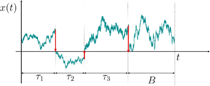
Figure 1: Schematics of BM with resetting. Since BM is Markovian the backward recurrence time $B$ controls the position of the restarted walker at time $t$. For short times, statistical properties of $B$ will obviously depend on $t$, the only exception is when the waiting times are exponentially distributed. If the time $t$ is long a steady state of the random variable $B$ is found provided that the mean time between resets is finite. This in turn will determine the steady state statistical properties of the stochastic process $x(t)$. When the mean time between resetting events diverges we are in the domain of infinite ergodic theory.

We are interested in the PDF of the position of the particle at time $t$ denoted $\rho(x,t)$. Let $x(t)$ be the stochastic process describing the location of the particle. Since BM is a Markovian process, hence $x(t)$ is connected to the time the last reset to $x=0$ was made. This last reset event is at time $t-B$ and $B$ is called the backward recurrence time (see schematics in Fig. 1). Clearly $B$ is a RV, whose statistical properties in general depend on $t$ while $0\leq B\leq t$. In the process just described $x(t)=x^{f}(B)$ where $x^{f}(B)$ is the position of a reset free BM at time $B$, with the initial position $x=0$. Hence from the well known properties of BM, $x(t)$ for the resetting process, is a product of two independent random variables $\sqrt{B}$ and $\xi$, namely

$$x(t)=(DB)^{1/2}\xi$$ (2)

where $\xi$ is a Gaussian RV with zero mean and variance $\langle\xi^{2}\rangle=2$.

The backward time is defined according to

$$\sum_{i=1}^{N}\tau_{i}+B=t,$$ (3)

where $N$ is the random number of resets in the time interval $(0,t)$, see again schematics in Fig. 1. Then using the Fourier $x\to k$ transform of $\rho(x,t)$ and Eq. (2), ${\cal F}[\rho(x,t)]=\langle\langle\exp(ik\sqrt{DB}\xi)\rangle_{\xi}\rangle_{B}=\langle\exp(-k^{2}DB)\rangle_{B}$ were we used the fact that $B$ and $\xi$ are independent RVs, and that the PDF of $\xi$ is Gaussian. We then have

$${\cal F}[\rho(x,t)]=\int_{0}^{t}f(B,t)\exp(-k^{2}DB){\rm d}B$$ (4)

and as mentioned $f(B,t)$ is the PDF of $B$. Hence inverting back to $x$ space, the formal solution to the problem reads

$$\rho(x,t)=\int_{0}^{t}f(B,t)G(x,B){\rm d}B.$$ (5)

Luckily statistics of $B$ are well studied in the context of renewal theory, in particular the PDF $f(B,t)$ is studied in Godreche2001 . Specifically, the Laplace transform of $f(B,t)$ is given in terms of the Laplace transform of $\psi(\tau)$ in Godreche2001 and some further details will be provided below.

To study non-equilibrium steady states we soon focus on the long time limit of Eq. (5). Before doing so we note that the approach is not limited to BM in dimension-one, in essence many other transformation of $B$ might be considered, for example consider BM in a force field Pal2015 ; Ray2020 with resetting, or anomalous diffusion Masolivier2019 ; Bordova2019 ; Bordova2020 ; Mendez2021 ; Majumdar2022 ; Weron2022 , or deterministic processes etc. And as explained below the waiting time strategy just described, is identical to a much studied time varying rate approach Pal2016 ; Eule2016 . In all these problems the backward recurrence time plays a crucial role hence we will soon recap some of its properties.

In this paper we will focus on two classes of resetting processes. The first are processes with a smooth PDF $\psi(\tau)$ of the reset times, when the positive integer moments of the waiting times are finite. The most studied example is $\psi(\tau)=\exp(-\tau)$ for $\tau>0$ and we have set here the mean waiting time to be unity. We will also discuss briefly deterministic resetting $\psi_{{\rm det}}(\tau)=\delta(\tau-\tau_{{\rm det}})$, which is a special case. The second class of PDFs have a power law tail for large $\tau$

$$\psi(\tau)\sim(\tau_{0})^{\alpha}\tau^{-1-\alpha},\ \ \mbox{and}\ \ 0<\alpha<1.$$ (6)

As well known these PDFs belong to the domain of attraction of Lévy’s laws and the big jump principle Burioni holds instead of standard large deviation theory. In particular the mean waiting time diverges and in that sense the process is scale free. Other cases, like $\alpha=1$ and $1<\alpha<2$ are also of interest, but due to space considerations will not be presented here.

III Statistics of the backward recurrence time

In the long time limit the measurement time $t$ typically falls in a time interval which is longer than the average, see viewpoint on this issue in Pal2022 . This time interval straddling time $t$ is a sum of the forward recurrence time (time between $t$ and the first renewal after $t$) and the mentioned backward time (time between $t$ and the previous reset event). The steady state (ss) PDF of $B$ for non-lattice PDFs of resetting time is Godreche2001 ; Dynkin1955

$$f^{{\rm ss}}(B)={1-\int_{0}^{B}\psi(\tau){\rm d}\tau\over\langle\tau\rangle}$$ (7)

and $\langle\tau\rangle=\int_{0}^{\infty}\tau\psi(\tau){\rm d}\tau$ is the mean time between resetting. When $\psi(\tau)$ is exponentially decaying, the distribution of $B$ is $f(B)=\exp(-B)$, and hence the same as that of the distribution of the time between resetting. More precisely in the long time limit $f(B,t)$ reaches this steady state, provided that the mean time between resets $\langle\tau\rangle$ is finite (class number one above) and hence

$$\lim_{t\to\infty}\langle\tau\rangle f(B,t)=1-\int_{0}^{B}\psi(\tau){\rm d}\tau={\cal I}^{{\rm ss}}(B).$$ (8)

Here we call ${\cal I}^{{\rm ss}}(B)$ the invariant steady state which is dimensionless and also a perfectly normalizable function. What happens when $\langle\tau\rangle$ diverges?

If $\alpha<1$ (class 2) then as shown by Wang et al. the PDF of $B$ satisfies Wanli2018

$$\lim_{t\to\infty}\langle\tau^{*}(t)\rangle f(B,t)=1-\int_{0}^{B}\psi(\tau){\rm d}\tau={\cal I}^{\infty}(B).$$ (9)

For a brief recap of this and other basic results see Sec. VI. Eq. (8) and Eq. (9) appear similar, but they are not. In Eq. (9) $\langle\tau^{*}(t)\rangle\propto t^{1-\alpha}$ is increasing with measurement time (see below). Still the invariant densities ${\cal I}^{{\rm ss}}(B)$ and ${\cal I}^{\infty}(B)$ have the same functional dependence on the waiting time PDF, though ${\cal I}^{\infty}(B)$ is called an infinite invariant density since it is not a normalizable function. Since by definition on the left hand side of Eq. (9) we take a perfectly normalised function $f(B,t)$ and multiply it by a monotonically increasing function of time and take the long time limit, the integration of ${\cal I}^{\infty}(B)$ over $B>0$ diverges. This is because ${\cal I}^{\infty}(B)\propto B^{-\alpha}$ and $0<\alpha<1$ and hence it is a non-integrable function due to its large $B$ behavior.

Eqs. (8) and (9) are valid for any finite $B$ in the limit of long measurement times. However, especially when $0<\alpha<1$ the case when $B$ scales with measurement time must also be considered, namely when $B\propto t$ and $t$ is made large. This limit was studied by Dynkin who found Dynkin1955 ; Godreche2001

$$f(B,t)\sim{1\over t}{\rm Dyn}\left({B\over t}\right),$$ (10)

and the scaling function reads

$${\rm Dyn}(y)={\sin\pi\alpha\over\pi}{1\over y^{\alpha}(1-y)^{1-\alpha}},\ \ \ 0<y<1.$$ (11)

This formula shows that the most likely events, are obtained when $y\sim 0$ or $y\sim 1$, where the Dynkin PDF diverges, corresponding to either very short $B$ compared to $t$ or $B$ of the order of $t$. Note that when $\alpha=1/2$ we find the arcsine law attributed to P. Lévy.

We see that for $\alpha<1$ we have two limiting laws, one for $B$ fixed and measurement time long, and the other when the ratio $B/t$ is fixed. The use of these laws, for example for the calculations of expectation values, depends on the observable of interest. We will later study observables which are integrable with respect to the infinite density, and show how infinite ergodic theory plays a special role for the non-equilibrium steady states.

Note that Eq. (9) and Eq. (11) are related as they have to match. To see this, using Dynkin limit theorem, with $B\ll t$ we have

$$f(B,t)\sim{1\over t}{\sin\pi\alpha\over\pi}{1\over(B/t)^{\alpha}}.$$ (12)

On the other hand using Eq. (6), ${\cal I}^{\infty}(B)\sim(\tau_{0})^{\alpha}B^{-\alpha}/\alpha$ for large $B$. Since $f(B,t)\sim{\cal I}^{\infty}(B)/\langle\tau^{*}(t)\rangle=(\tau_{0})^{\alpha}B^{-\alpha}/\alpha\langle\tau^{*}(t)\rangle$ we easily find

$$\langle\tau^{*}(t)\rangle={\pi(\tau_{0})^{\alpha}\over\alpha\sin\pi\alpha}t^{1-\alpha}.$$ (13)

This is exactly the expression found in Wanli2018 . Note that roughly speaking $\langle\tau^{*}(t)\rangle$ is a mean time between resets, in the sense that if we integrate only up to $t$ $\langle\tau^{*}(t)\rangle\propto\int^{t}\tau\psi(\tau){\rm d}\tau\sim t^{1-\alpha}$ as indeed we have found. More precisely, let $\langle N\rangle$ be the averaged number of resets in the time interval $(0,t)$. Then in the long time limit Godreche2001

$${{\rm d}\langle N\rangle\over{\rm d}t}\sim\left\{\begin{array}[]{c c}{1\over\langle\tau^{*}(t)\rangle}&{\mbox{w}hen}\ \ 0<\alpha<1\\ {1\over\langle\tau\rangle}&{\mbox{o}therwise}.\end{array}\right.$$ (14)

Thus $1/\langle\tau\rangle$ and $1/\langle\tau^{*}(t)\rangle$ are the long time rates of the underlying renewal process. Namely $d\langle N\rangle$, which is the probability of observing a reset event in the time interval $(t,t+{\rm d}t)$, is given by ${\rm d}t/\langle\tau^{*}(t)\rangle$ for $0<\alpha<1$ and by ${\rm d}t/\langle\tau\rangle$ otherwise. Thus using Eqs. (8,9,13) we summarize

$$\lim_{t\to\infty}{f(B,t)\over\left({{\rm d}\langle N\rangle\over{\rm d}t}\right)}=S(B)$$ (15)

and $S(B)$ is the survival probability, i.e. the probability of not performing a reset in time $B$

$$S(B)=1-\int_{0}^{B}\psi(\tau){\rm d}\tau=\int_{B}^{\infty}\psi(\tau){\rm d}\tau.$$ (16)

Eq. (15) gives the invariant density of the backward time, be it either normalizable or not.

IV NESS

IV.1 Normalized invariant density

We now consider thin tailed waiting time PDFs of the first class. The non-equilibrium steady state, $\rho^{{\rm ss}}(x)$ is based on the long time limit of the distribution of $B$ using Eqs. (5,7,16)

$$\lim_{t\to\infty}\langle\tau\rangle\rho(x,t)=\langle\tau\rangle\rho^{{\rm ss}}(x)=\int_{0}^{\infty}S(B){\exp\left(-{x^{2}\over 4DB}\right)\over\sqrt{4\pi DB}}{\rm d}B.$$ (17)

For example setting $D=1/2$ and using $\psi(\tau)=\exp(-\tau)$ so $\langle\tau\rangle=1$ and hence $S(B)=\exp(-B)$ we find the result in Evans2011 $\rho^{{\rm ss}}(x)=\exp[-\sqrt{2}|x|]/\sqrt{2}$, which exhibits the typical non-analytical behavior at $|x|\to 0$. The latter is a rather general feature of NESS, since if we expand the Gaussian in Eq. (17) to second order in $x$, the $x^{2}$ term will diverge, since $S(0)=1$ and $B^{-3/2}$ is non integrable at $B\rightarrow 0$. Pal et al, Pal2016 derived a formula for the steady state, which is identical to Eq. (17) without invoking the backward recurrence time and using Laplace transforms (see also Eule2016 ). In Appendix A we make the comparison between the two results and explain the different notations.

IV.2 Non-normalized invariant density $1/2<\alpha<1$

For the second class of PDFs given in Eq. (6), we again start with Eq. (5) which gives $\rho(x,t)=\langle G(x,B)\rangle$, here the average is with respect to the distribution of the backward time $B$. As we soon explain, the Gaussian function $G(x,B)$ can be either integrable with respect to the infinite density of $B$ when $1/2<\alpha<1$ or not corresponding to $0<\alpha<1/2$. The case $\alpha=1/2$ marks a transition in the ergodic properties of the system. This is in addition to the marginal case $\alpha=1$ that marks a second transition to a normalized steady state and perfectly standard ergodic theory.

Consider $1/2<\alpha<1$ and insert Eq. (9) in Eq. (5) using Eq. (16). We find an expression which looks similar to Eq. (17)

$$\lim_{t\to\infty}\langle\tau^{*}(t)\rangle\rho(x,t)=\int_{0}^{\infty}S(B){\exp\left(-{x^{2}\over 4DB}\right)\over\sqrt{4\pi DB}}{\rm d}B=\tilde{{\cal I}}^{\infty}(x).$$ (18)

Of course the major difference if compared with Eq. (17) is that on the left hand side of Eq. (18) we have the effective time dependent mean resetting time $\langle\tau^{*}(t)\rangle$. To see that the integral on the right hand side exists, namely that $G(x,B)$ is indeed integrable with respect to the non-normalized state ${\cal I}^{\infty}(B)$ if $1/2<\alpha<1$, note that for large $B$, $S(B)\propto B^{-\alpha}$ and hence the integral in Eq. (18) converges or diverges if $1/2<\alpha<1$ or $0<\alpha<1/2$, respectively. The function $\tilde{{\cal I}}^{\infty}(x)$ defined in Eq. (18) is the non-normalizable non-equilibrium steady state of $x$, as the integration over $x$ of this function diverges. The formula is valid for any finite $x$ in the long time limit. Note that we use the convention that the argument in the parenthesis defines the infinite density of interest, thus ${\cal I}^{\infty}(B)$ is the infinite density of $B$ while $\tilde{{\cal I}}^{\infty}(x)$ is the infinite density of $x$.

IV.3 Scaling solution $0<\alpha<1$

When $x\propto\sqrt{t}$ and both $x$ and $\sqrt{t}$ are large a different approach is needed. Inserting Dynkin’s limit theorem Eq. (10) in Eq. (5) we find

$$\rho(x,t)\sim{1\over t}\int_{0}^{t}\mbox{Dyn}\left({B\over t}\right)G(x,B){\rm d}B.$$ (19)

Making this equation explicit, we use Eqs. (1,11) and simple change of variables to obtain

$$\rho(x,t)\sim{g_{\alpha}\left(\xi\right)\over\sqrt{2Dt}}\ \ \mbox{with}\ \ \xi=|x|/\sqrt{2Dt}.$$ (20)

The scaling here is $x\propto\sqrt{t}$ hence it is diffusive, and this limit describes what we may call the typical events, further it is valid for $0<\alpha<1$. The scaling function is

$$g_{\alpha}(\xi)={\sin\pi\alpha\over\pi}\int_{0}^{1}{\exp\left(-{\xi^{2}\over 2\eta}\right)\over\eta^{\alpha}(1-\eta)^{\alpha}}{{\rm d}\eta\over\sqrt{2\pi\eta}}.$$ (21)

This function unlike the invariant densities Eqs. (17,18) does not depend on the fine details of the model, i.e. on the waiting time PDF, beyond the parameter $\alpha$. After change of variables, we find

$$g_{\alpha}(\xi)={1\over\sqrt{2\pi}\Gamma(1-\alpha)}U\left(\alpha,{1\over 2}+\alpha,{\xi^{2}\over 2}\right)e^{-\xi^{2}/2}$$ (22)

where we used the Tricomi function also called the Kummer function of the second kind. This equation was derived with a different approach by Nagar and Gupta Gupta2016 . Here we have emphasized the connection between the resetting problem and Dynkin’s limit theorem. We think this is worth while, since in many fat tailed resetting problems, the scaling solution for the diffusing particle will depend on this law, for example if we replace the Gaussian propagator of free diffusion $G(x,B)$ with a propagator of anomalous type, similar laws will follow.

The behavior of the scaling solution in vicinity of the resetting point $x=0$ is of interest. Exploiting the small $\xi$ limit of the Kummer function we have Abr

$$g_{\alpha}(\xi)\sim\left\{\begin{array}[]{c c}{2^{\alpha-1}\over\sqrt{\pi}}{\Gamma\left(\alpha-{1\over 2}\right)\over\Gamma\left(1-\alpha\right)\Gamma\left(\alpha\right)}{1\over\xi^{2\alpha-1}}&\ {1\over 2}<\alpha<1\\ &\\ -{1\over\sqrt{2}\pi^{3/2}}\left[2\ln\xi-\gamma-3\ln 2\right]&\ \alpha={1\over 2}\\ &\\ {\Gamma\left({1\over 2}-\alpha\right)\over\sqrt{2}\Gamma(1-\alpha)\pi}&\ 0<\alpha<{1\over 2}\end{array}\right.$$ (23)

where $\gamma$ is the Euler-Mascheroni constant. We see that the scaling solution, when $\xi\to 0$, exhibits a transition at $\alpha=1/2$. When $0<\alpha<1/2$ the scaling function at $x=0$, namely $g_{\alpha}(\xi=0)$ is a constant, and as Eq. (22) shows this constant diverges when $\alpha\to 1/2$ from below. Further when $\alpha\to 0$ we find $\rho(x=0,t)\sim g_{0}(\xi=0)/\sqrt{2Dt}=1/\sqrt{4\pi Dt}$ which is the expected result since for $\alpha\to 0$ the solution $\rho(x,t)$ is the Gaussian PDF describing free BM.

As a stand alone, Eqs. (20,23) indicate that $\rho(x,t)\to\infty$ when $x\to 0$ (or $\xi\to 0)$ and when $1/2<\alpha<1$. Clearly this is an unphysical effect. The density of the particles $\rho(x,t)$, for thin tailed distributions on the origin $x=0$, is always finite for any $t>0$, and with power law distributed times between the resetting, we expect an even lower density, since particles can escape to larger distances. Mathematically, the small $x$ regime is exactly the regime where the infinite density solution, namely Eq. (18) with $\rho(x,t)\sim\tilde{{\cal I}}^{\infty}(x)/\langle\tau^{*}(t)\rangle$ plays an important role (recall that the latter formula is valid for finite $x$). In this sense the non-normalized state cures an unphysical feature of the scaling solution Eq. (22). To study this issue let

$$\psi(\tau)=\alpha(t_{0})^{\alpha}\tau^{-(1+\alpha)}\ \mbox{for}\ \tau>t_{0},$$ (24)

otherwise it is zero, hence from Eq. (6) $(\tau_{0})^{\alpha}=\alpha(t_{0})^{\alpha}$. Using the non-normalized state Eq. (18), for $x=0$

$$\rho(0,t)\sim{2\alpha\over 2\alpha-1}{\sin\pi\alpha\over\pi^{3/2}}{(\tau_{0}/\alpha^{1/\alpha})^{1/2-\alpha}\over\sqrt{D}t^{1-\alpha}}.$$ (25)

Here we see that when $\alpha\to 1$ the time dependence vanishes as we approach the standard behavior of thin tailed statistics, and when $\alpha\to 1/2$ the solution decays like one over square root of time, as expected from diffusion. Returning to Eq. (23), this equation is valid for length scales $x>C(\alpha)\sqrt{D\tau_{0}}$ where $C(\alpha)$ depends on the exponent $1/2<\alpha<1$ and in principle it can be estimated by equating Eq. (25) and Eq. (23).

More technically, one can verify that the large $x$ expansion of $\rho(x,t)$ in Eq. (18), is exactly the same as the small $x$ limit of the scaling solution employing Eq. (23). Thus the infinite density solution for large $x$ matches the scaling solution for small $x$, as it should.

IV.4 Non-normalized invariant density $0<\alpha<1/2$

Finally, what is the infinite density for $0<\alpha<1/2$? Using Eq. (20)

$$\lim_{t\to\infty}\sqrt{2Dt}\rho(x,t)=g_{\alpha}(0)=\tilde{{\cal I}}^{\infty}(x).$$ (26)

and the constant $g_{\alpha}(0)$ is given in Eq. (23). Here the infinite density is $x$ independent so it is clearly a non-normalizable function, as the integration over $x$ from minus infinity to infinity diverges. The infinite density here does not depend on the structure of the waiting time PDF, and hence is very different if compared to the invariant densities found for thin tailed distribution, namely the normalized state, and that found in Eq. (18).

Note that in Eq. (18) we used the ever increasing time scale $\langle\tau^{*}(t)\rangle$ to define the non-normalized state, while for the case case $0<\alpha<1/2$ we used the diverging length scale $\sqrt{2Dt}$. These infinite densities are certainly not probability densities and their use will be explained later, in fact the units of the infinite density can be either the inverse of time or inverse of length, depending on the value of $\alpha$. In general infinite densities are defined up to some arbitrary constant (since these functions are not normalized we have some freedom in the definition). This does not pose any problem, as long as one recalls the basic definitions. For example to visualise the infinite density in simulations, we plot the density $\rho(x,t)$ times $\sqrt{2Dt}$ for finite $x$ and increase time, the solution in the long time limit will approach $\tilde{{\cal I}}^{\infty}(x)$ for $0<\alpha<1/2$. Or we plot $\langle\tau^{*}(t)\rangle\rho(x,t)$ for finite range of $x$, and then as we increase measurement time the solution will approach the asymptotic infinite density Eq. (18). Of course as $t$ is increased, most of the particles are actually diffusing far from the origin. Thus in practice if $t$ is too long and the number of trajectories in simulation not large enough, it will be hard to visualise the infinite densities. To meet this sampling challenge we plot now the non-normalized states for representative case.

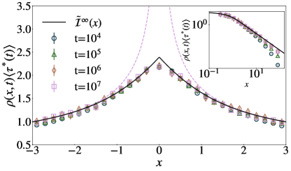
Figure 2: The infinite density versus $x$ for $\alpha=3/4$. In simulation we plot the histogram for the density $\rho(x,t)$ multiplied by $\langle\tau^{*}(t)\rangle$ versus $x$. Increasing time we see that results converge to the theoretical prediction namely the solid line presenting the infinite density $\tilde{{\cal I}}^{\infty}(x)$, Eq. (31). For large $x$, $\tilde{{\cal I}}^{\infty}(x)\simeq 1/|x|^{1/2}$, Eq. (32), hence this invariant density is not normalized. The infinite density exhibits a typical cusp on the origin. Also shown is the scaling solution Eq. (23) for time $10^{7}$ (dashed line). The latter is a good approximation for diffusive scales, namely when $x$ of the order $t^{1/2}$, but for small $x$ presented here, the scaling solution clearly fails. We use the Pareto PDF of times between resets with $t_{0}=1$ and $D=1/2$. We have used $1.3\cdot 10^{6}$ trajectories. Inset: we present the large $x$, and the data for various times does not collapse on a master curve, unlike the small $x$ shown in the main figure.

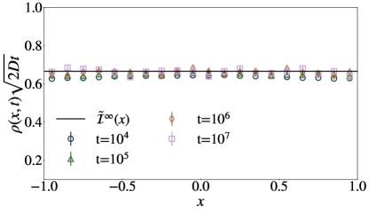
Figure 3: The infinite density versus $x$ for $\alpha=1/4$. In simulation we plot the histogram for the probability density $\rho(x,t)$ multiplied by $\sqrt{2Dt}$, unlike the case $\alpha>1/2$ where we use $\langle\tau^{*}(t)\rangle$, as shown in Fig. 2. The solid line is the theory, the infinite density $\tilde{{\cal I}}^{\infty}(x)$ Eq. (26), namely $\tilde{{\cal I}}_{1/4}(x)=g_{1/4}(0)=\Gamma(1/4)/\sqrt{2}\Gamma(3/4)\pi\simeq 0.6659$. Now the infinite density is simply a constant, and the cusp found for $\alpha=3/4$ in Fig. 2, is not present. Further, clearly a constant invariant density is not normalized. We use the Pareto PDF of times between resets with $t_{0}=1$ and $D=1/2$. We have used $10^{8}$ trajectories.

IV.5 Examples

As a specific example consider the Pareto PDF of resetting times $\psi(\tau)=\alpha\tau^{-1-\alpha}\ \mbox{when}\ 1<\tau$ otherwise $\psi(\tau)=0$, hence $t_{0}=1$ in Eq. (24). We also set $D=1/2$. In this case

$$\langle\tau^{*}(t)\rangle\sim(\pi/\sin\pi\alpha)t^{1-\alpha},$$ (27)

where we used Eqs. (6, 13). It follows from Eq. (18)

$$\tilde{{\cal I}}^{\infty}(x)=\int_{0}^{1}{\exp\left(-{x^{2}\over 2B}\right)\over\sqrt{2\pi B}}{\rm d}B+\int_{1}^{\infty}B^{-\alpha}{\exp\left(-{x^{2}\over 2B}\right)\over\sqrt{2\pi B}}{\rm d}B.$$ (28)

For $x=0$ we find

$$\tilde{{\cal I}}^{\infty}(0)=\sqrt{{2\over\pi}}{\alpha\over\alpha-{1\over 2}}.$$ (29)

Hence for $1/2<\alpha<1$ the density on the origin

$$\rho(0,t)\sim{\tilde{{\cal I}}^{\infty}(0)\over\langle\tau^{*}(t)\rangle}$$ (30)

is decreasing with time, and the divergence of the scaling solution Eq. (23) at $\xi=x=0$ is not relevant, since as mentioned that solution is not valid in this regime. For the example $\alpha=3/4$ Eq. (28) gives

$$\tilde{{\cal I}}^{\infty}_{\alpha=3/4}(x) = |x|\left({\rm erf}\left({|x|\over\sqrt{2}}\right)-1\right)+\sqrt{{2\over\pi}}e^{-{x^{2}\over 2}}$$ (31)

$$+ {\Gamma\left({1\over 4}\right)-\Gamma\left({1\over 4},{x^{2}\over 2}\right)\over 2^{1/4}\sqrt{\pi}\sqrt{|x|}}$$

where we use the error function and the incomplete Gamma function. This invariant density is plotted in Fig. 2 together with finite time numerical simulations. As shown the infinite density exhibits a cusp on the reseting point $x=0$, which is found also for resetting problems with a normalized invariant density. For large $x$ we have

$$\tilde{{\cal I}}^{\infty}_{\alpha=3/4}(x)\sim{\Gamma\left({1\over 4}\right)\over 2^{1/4}\sqrt{\pi}\sqrt{|x|}}.$$ (32)

This expression can be shown to match the small $x$ behavior of the scaling solution Eq. (23). Similarly in Fig. 3 we study the case $\alpha=1/4$. As predicted by theory the infinite density is structureless, namely it is equal to a constant. This is clearly unlike what we see in Fig. 2, so the transition at $\alpha=1/2$ is evident.

IV.6 Efficient sampling

When simulating invariant densities of restart processes one may follow at least two strategies. The first is to construct the renewal process, namely using a simple program and a given $\psi(\tau)$, we find the sequence $\{\tau_{1},\tau_{2},...,B\}$, for a given measurement time $t$. Using $B$ it is then easy to find $x_{{\rm free}}(B)$ which denotes the reset free dynamics at time $B$. As mentioned this is the same as the coordinate of the walker with resetting at time $t$. This method is by far more efficient if compared with continuously recording full trajectories of the reset process. This is clearly the case as $B<t$. Further, if we have the measurement free propagator as for the case considered here, then given $B$ one may find $x_{{\rm free}}(B)=x(t)$ without simulating the trajectory. We have generated Fig. 2 using both methods, and as expected the results are the same, though the first method is by far more efficient.

V The moments

V.1 Thin tailed distributions

Using Eq. (2) the moments of the process satisfy

$$\langle x^{2m}(t)\rangle=D^{m}\langle\xi^{2m}\rangle\langle B^{m}\rangle$$ (33)

and here $m=0,1,2,..$. We used the fact that odd moments of $x(t)$ vanish from symmetry. Recall that the PDF of $\xi$ is Gaussian with zero mean and variance equal $2$ namely $\mbox{PDF}(\xi)=\exp(-\xi^{2}/4)/\sqrt{4\pi}$. In the normalized steady state, namely when we deal with thin tailed PDFs of resetting times, the moments of $B$ become time independent and so do the moments of $x(t)$. For example

$$\langle x^{2}\rangle_{{\rm ss}}=2D\langle B\rangle_{{\rm ss}}.$$ (34)

and in general $\langle x^{2m}\rangle_{\rm ss}=D^{m}\langle\xi^{2m}\rangle\langle B^{m}\rangle_{{\rm ss}}$, where

$$\langle\xi^{2m}\rangle={4^{m}\Gamma(m+1/2)\over\sqrt{\pi}}.$$ (35)

In turn the moments of $B$ are determined by the moments of $\psi(\tau)$ using Eq. (7). We use the Laplace transform $\hat{\psi}(s)=\int_{0}^{\infty}\exp(-s\tau)\psi(\tau){\rm d}\tau$, and similarly $\hat{f}_{{\rm ssB}}(s)$ is the Laplace pair of $f_{{\rm ss}}(B)$. Using the convolution theorem and Eq. (7)

$$\hat{f}_{{\rm ssB}}(s)={1-\hat{\psi}(s)\over s\langle\tau\rangle}.$$ (36)

The Laplace transforms are also moment generating functions, hence expanding for small $s$

$$\hat{\psi}(s)=1-s\langle\tau\rangle+s^{2}{\langle\tau^{2}\rangle\over 2}+\cdots$$ (37)

where $\langle\tau^{m}\rangle$ are the moments of the times between resets and similarly

$$\hat{f}_{{\rm ssB}}(s)=1-s\langle B\rangle_{{\rm ss}}+s^{2}{\langle B^{2}\rangle_{{\rm ss}}\over 2}+\cdots.$$ (38)

Inserting Eqs. (37,38) in Eq. (36) we find

$$1-s\langle B\rangle_{{\rm ss}}+s^{2}{\langle B^{2}\rangle_{{\rm ss}}\over 2}+\cdots=$$

$${1-\left(1-s\langle\tau\rangle+s^{2}{\langle\tau^{2}\rangle\over 2}-{s^{3}\langle\tau^{3}\rangle\over 3!}+\cdots\right)\over s\langle\tau\rangle}.$$ (39)

Comparing terms of the same order we have $\langle B\rangle_{{\rm ss}}=\langle\tau^{2}\rangle/(2\langle\tau\rangle)$, $\langle B^{2}\rangle_{{\rm ss}}=\langle\tau^{3}\rangle/(3\langle\tau\rangle)$ and in general $\langle B^{m}\rangle_{{\rm ss}}=\langle\tau^{m+1}\rangle/[(m+1)\langle\tau\rangle]$. From Eq. (33) we find

$$\langle x^{2}\rangle_{{\rm ss}}=D{\langle\tau^{2}\rangle\over\langle\tau\rangle}$$ (40)

and more generally

$$\langle x^{2m}\rangle_{{\rm ss}}={4^{m}\over(m+1)}{\Gamma\left(m+{1\over 2}\right)\over\sqrt{\pi}}{D^{m}\langle\tau^{m+1}\rangle\over\langle\tau\rangle}.$$ (41)

V.2 Sharp restart is the squeezed state

A natural question is to what extent can we squeeze the steady state distribution of $x$? Of course fast resetting will simply put the particle always on the origin. If we fix $\langle\tau\rangle$ to some non-zero value, the narrowest steady state § PDF of $x$, will be naively found when $\psi_{{\rm det}}(\tau)=\delta(\tau-\langle\tau\rangle)$. This strategy is called sharp restart and its NESS was studied in Eule2016 . Further, sharp restart is optimal for search Pal2017 ; Eliazar2020 hence studied extensively Yin . In this case the variance of $x$, is $\langle x^{2}\rangle_{{\rm ss}}=D\langle\tau\rangle$ which is smaller that any other $\langle x^{2}\rangle_{{\rm ss}}$ found with another choice of $\psi(\tau)$, since in general $\langle\tau^{2}\rangle/\langle\tau\rangle\geq\langle\tau\rangle$ and hence sharp restart gives the minimum of the dispersion.

V.3 No NESS for Sharp restart

However, sharp restart implies that the PDF $\psi(\tau)$ being non-smooth is in fact not in the domain of the theory discussed here, as we mentioned from the start. For sharp restart there is no NESS. To see this note that at any time $t$ slightly larger then an integer times $\langle\tau\rangle$, the particle is on $x\simeq 0$. In contrast just before these times, the PDF of $x$ is a Gaussian with variance, $2D\langle\tau\rangle$. In short, for stroboscopic resetting, that starts at time $t=0$, we have no NESS, in the sense that the PDF of $x$ is time dependent, with a periodicity which is the sharp time between resets. One can claim that if the restart is nearly sharp, i.e. if we have a narrow but analytical PDF of $\psi(\tau)$ around some $\langle\tau\rangle$, namely some small uncertainty in the resetting times, the process will converge to the NESS. While this is correct, this convergence will take very long, and the narrower is the PDF of reset times, around the sharp reset time $\langle\tau\rangle$, the longer will the relaxation towards the NESS will be. Another option of obtaining a NESS, for lattice PDFs of resetting time, is to randomize the initial clock, however this option is not part of this work.

V.4 Fat-tailed distributions

Eq. (33) is still valid when $0<\alpha<1$. Noticing that $B^{m}$ is non-integrable with respect to the infinite density Eq. (9), since the later decays like $B^{-\alpha}$ for large $B$, we realize that the moments are determined by the large $x$ behavior of the propagator $\rho(x,t)$, when the scaling presented in Eq. (22) is diffusive. One may in principle find the moments $\langle x^{2m}(t)\rangle$ using the properties of the Kummer function, however there is no need for that. Eq. (33) is still valid and the moments increase with time, for example

$$\langle x^{2}(t)\rangle\sim 2D\langle B(t)\rangle_{{\rm Dyn}}.$$ (42)

In turn the moments of the backward recurrence time are obtained using Dynkin’s limiting law Eq. (10,11). For $m=0,1,..$ we use

$$\int_{0}^{1}{y^{m-\alpha}\over(1-y)^{1-\alpha}}{\rm d}y={\Gamma(\alpha)\Gamma(m-\alpha+1)\over m!},$$ (43)

and hence

$$\langle B^{m}(t)\rangle_{{\rm Dyn}}\sim{\Gamma(m-\alpha+1)\over m!\Gamma(1-\alpha)}t^{m}.$$ (44)

Then we find the diffusive type of scaling for the moments

$$\langle x^{2m}(t)\rangle\sim D^{m}\langle\xi^{2m}\rangle\langle B^{m}(t)\rangle_{{\rm Dyn}}$$ (45)

which is made explicit with Eqs. (35,44). In the limit $\alpha<<1$ we have $\langle B^{m}(t)\rangle_{{\rm Dyn}}\sim t^{m}$ since then the resetting is extremely sparse, and as expected the moments $\langle x^{2m}(t)\rangle$ are determined by free diffusion.

We see that the moments of the process are determined by the scaling solution of $B$ Eq. (10), and hence are not sensitive to the details of the waiting time PDF $\psi(\tau)$. This is because the moments explore the large $x$ part of the density $\rho(x,t)$. Another class of observables, considered in the next section, are integrable with respect to the non-normalized state. And these do not exhibit diffusive scaling, and their ergodic properties are of special interest as they are related to the non-normalized NESS found here.

VI Fractional Integral Equation for the density

The goal of this section is to find a valid approximation for $\rho(x,t)$ in the limit of long times, this should hold both for large and small $x$. As we showed the infinite density approach works well for small $x$, the scaling solution works well for large $x$, so now we want to marry the two solutions, using a uniform approximation. Further, close to the transition $\alpha=1/2$ the convergence to asymptotic results is extremely slow, and this can be overcome with the uniform approximation.

Figure 4: Numerical simulations for the PDF of the rescaled backward recurrence time $0<B/t<1$ for $\alpha=1/2$ converge to the arcsine law. Deviations from this well known behavior are presented in figure 5

We focus on fat tailed PDFs of waiting time Eq. (6), $\psi(\tau)\sim(\tau_{0})^{\alpha}\tau^{-1-\alpha}$, and $0<\alpha<1$. The Laplace transform of this function, for small $s$ is provided by WeiWang2021 ; Godreche2001 ; Klafter

$$\hat{\psi}(s)\sim 1-b_{\alpha}s^{\alpha}+\cdots,\;\text{where}\;\;b_{\alpha}=(\tau_{0})^{\alpha}\Gamma(1-\alpha)/\alpha$$ (46)

We start with a recap of a handful of known results from the field of renewal processes Godreche2001 ; Wanli2018 ; Cox1962 .

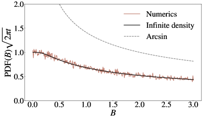
Figure 5: Numerical simulations for the PDF of the backward recurrence time $B$, multiplied by $\langle\tau^{*}(t)\rangle$, perfectly match the prediction based on the infinite invariant density Eq. (54). Note that $0<B<3$ while $t=10^{4}$ hence the figure presents the small $B$ behavior of the density. Here $\alpha=1/2$ hence the arcsine law Eq. (11) describes the typical fluctuations of $B$, however as shown and as expected it fails here (it works fine in the large $B$ regime). As a stand alone the arcsine law predicts that the density will diverge when $B\to 0$, which is clearly not the case for any finite $t$. In simulations we use $10^{7}$ realizations of the renewal process. The PDF of waiting times is given in Eq. (53) hence $\langle\tau^{*}(t)=\sqrt{2\pi t}$.

VI.1 Statistics of number of jumps

Let $P_{t}(N)$ be the probability for $N$ renewals in the period $(0,t)$. Using the convolution theorem of Laplace transform

$$\hat{P}_{s}(N)={1-\hat{\psi}(s)\over s}\left[\hat{\psi}(s)\right]^{N}$$ (47)

where $\hat{P}_{s}(N)$ is the Laplace $t\to s$ transform of $P_{t}(N)$. The mean number of jumps is $\langle N(t)\rangle$ and its Laplace pair reads Shlesinger1974

$$\langle\hat{N}(s)\rangle=\sum_{N=0}^{\infty}N\hat{P}_{s}(N)={\hat{\psi}(s)\over s\left[1-\hat{\psi}(s)\right]}.$$ (48)

Inserting Eq. (46) and inverting to the time domain

$$\langle N(t)\rangle\sim{\sin\pi\alpha\over\pi}\left({t\over\tau_{0}}\right)^{\alpha}$$ (49)

where we used the reflection formula for the $\Gamma$ function. Eq. (49) obeys (14).

VI.2 Backward time statistics

A technique for finding the distribution of the backward recurrence time is given in Godreche2001 , and it is based on double Laplace transforms. Let $f_{B}(t,B)$ be the PDF of $B$ and $\hat{f}_{B}(s,u)=\int_{0}^{\infty}{\rm d}t\int_{0}^{\infty}{\rm d}t\exp(-st-uB)f_{B}(t,B)$. Without any approximation

$$\hat{f}_{B}(s,u)={1-\hat{\psi}(s+u)\over s+u}{1\over 1-\hat{\psi}(s)}.$$ (50)

Here $\hat{\psi}(s+u)=\int_{0}^{\infty}\exp[-(s+u)\tau]\psi(\tau){\rm d}\tau$. In principle, if we can invert this formula to the double time domain, i.e. $t$ and $B$, we can find $\rho(x,t)$ using Eq. (5). Using Eq. (46), in the limit when $s\to 0$ and $u\to 0$ their ratio remaining finite

$$\hat{f}_{B}(s,u)\sim s^{-\alpha}(s+u)^{\alpha-1}.$$ (51)

This equation is independent of the fine details of the waiting time PDF besides $\alpha$. The inversion to the time domain is carried out in Godreche2001 yielding Dynkin’s limit theorem Eqs. (10,11). If the mean waiting time is finite, one uses Eq. (50) to find Eq. (8). Technically this is done by considering the limit $s\to 0$ while leaving $u$ fixed, which in turn, upon Laplace inversion, gives the long time limit of the problem.

Switching back to $0<\alpha<1$ such that the mean waiting time diverges, we consider Eq. (50) in the limit $s\to 0$ and $u$ finite Wanli2018 . Using Eq. (46)

$$\hat{f}_{B}(s,u)\sim{1-\hat{\psi}(u)\over u}{1\over b_{\alpha}s^{\alpha}}.$$ (52)

Inverting to the $(t,B)$ domain one finds Eq. (9). This describes the statistics of finite $B$ when $t$ is made large.

VI.3 Example $\alpha=1/2$

To demonstrate this behavior we consider an example. Let

$$\psi(\tau)={\exp\left(-{1\over 2\tau}\right)\over\sqrt{2\pi}\tau^{3/2}}$$ (53)

hence $\alpha=1/2$. This PDF is called the one sided Lévy stable distribution with index $1/2$, and is known as a van der Waals profile. In this case $\sqrt{\tau_{0}}=\sqrt{2/\pi}$ and $\langle\tau^{*}(t)\rangle=\sqrt{2\pi}t^{1/2}$. Using Eq. (9) we find

$$\lim_{t\to\infty}\langle\tau^{*}(t)\rangle f(B,t)=\mbox{Erf}\left({1\over\sqrt{2B}}\right),$$ (54)

where we introduced the error function. Recall that $\mbox{Erf}(1/\sqrt{2B})\sim 1$ for $B\to 0$ and $\mbox{Erf}(1/\sqrt{2B})\sim\sqrt{2/\pi}B^{-1/2}$ for large $B$. Hence the $B$ integration of this infinite invariant density diverges $\int_{0}^{\infty}\mbox{Erf}(1/\sqrt{2B}){\rm d}B=\infty$, due to the large $B$ limit.

We now consider finite time simulations to demonstrate the result. Generating the sequence of waiting times we find the statistics of $B$ using $10^{7}$ samples. The random waiting times are given by $\tau=1/G^{2}$, where $G$ is a Gaussian random variable with zero mean, whose PDF is $\exp[-G^{2}/2]/\sqrt{2\pi}$ Chambers . Generating such a normally distributed random variable with a computer program is a standard routine. Hence it is easy to generate the realizations of the renewal sequence and sample the random variable $B$ on a computer.

In Fig. 4 we plot the typical fluctuations of $B$ which are captured by Dynkin’s limit theorem, in fact since $\alpha=1/2$ we find the arcsine law. To do so we plot the histogram of the random variable $B/t$ which is clearly bounded in the unit interval. One sees the well known $U$ shaped histogram, meaning that small $B$ and large $B$ are by far more likely if compared to the mean which in the long time limit is $\langle B/t\rangle=1/2$. Small deviations from the asymptotic theory are observed on the left, and those are rare events.

To study these we focus on $0<B<3\ll t$. Here the infinite density is a valid approximation while the arcsine law is clearly invalid. In Fig. (5) we plot the normalized histogram for the backward time, namely the sample estimation of the PDF of $B$, multiplied by $\langle\tau^{*}(t)\rangle$ versus $B$. The numerical result matches $\mbox{Erf}(1/\sqrt{2B})$ without any fitting, indicating that also for finite time simulations the non-normalized result is a good approximation.

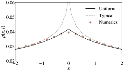
Figure 6: Numerics for the PDF of the position $x$ for an ensemble of particles undergoing the resetting process with $\alpha=1/2$. We focus on the small $x$ behavior, namely the vicinity of the resetting point $x=0$. The uniform approximation Eq. (59) perfectly matches the simulations, while the scaling solution Eq. (60), describing the typical fluctuations (large $x$) fails. Here $t=10^{3}$, the resetting time PDF is Eq. (53) and we used $10^{7}$ realizations.

VI.4 Uniform approximation

We have considered already the PDF of $B$, $f_{B}(B,t)$ in two limits. The typical behavior Eq. (10), when $B$ is scaled with time $t$ and the rare events Eq. (9). An important scale of $\psi(\tau)$, is roughly speaking the time beyond which $\psi(\tau)\sim(\tau_{0})^{\alpha}\tau^{-1-\alpha}$ is a valid approximation. For the Pareto distribution Eq. (24) this time scale is $t_{0}$ while for the one sided Lévy stable law Eq. (53) it is of order unity. For $B$ larger than this time scale the two solutions match, as mentioned already.

Now we present a simple uniform approximation for the density of $B$

$$f_{{\rm Uni}}(B,t)=\left\{\begin{array}[]{c c}S(B)\over\langle\tau^{*}(t-B)\rangle&\ 0<B<t\\ 0&\mbox{otherwise}.\end{array}\right.$$ (55)

This is obtained by matching the above mentioned two solutions. Eq. (55) holds for large $t$. By construction, for large $B$, we have $S(B)\sim(\tau_{0}/B)^{\alpha}/\alpha$ and hence this solution matches Dynkin’s limit theorem Eq. (10), while for small $B$ it yields Eq. (15)

We find the uniform approximation for the density of resetted particles. Using Eqs. (5, 55)

$$\rho_{{\rm Uni}}(x,t)=\int_{0}^{t}{\rm d}B{S(B)G(x,B)\over\langle\tau^{*}(t-B)\rangle}.$$ (56)

This is one of the main results of the paper as it provides both the large $x$ limit of the density $\rho(x,t)$ (described also by the scaling solution) and the small $x$ limit (given by the infinite density). Employing Eq. (13) for $\langle\tau^{*}(t)\rangle$ and the definition of the left sided fractional Riemann-Liouville integration

$${}_{0}D_{t}^{-\alpha}g(t)={1\over\Gamma(\alpha)}\int_{0}^{t}g(t^{\prime})(t-t^{\prime})^{\alpha-1}{\rm d}t^{\prime}$$ (57)

we find

$$(\tau_{0})^{\alpha}|\Gamma(-\alpha)|\rho_{\rm Uni}(x,t)=\ _{0}D_{t}^{-\alpha}\left[S(t)G(x,t)\right].$$ (58)

This equation holds far beyond the case of Brownian motion. It connects the survival probability, the propagator for reset free motion, and the density of the spreading particles. It describes both the small $x$ limit which is dominated by small $B$ statistics, as well as the scaling solution to the problem, discussed previously. Note that the inverse operation of the fractional integration is a fractional derivative, hence we may use Marchaut’s formula to find, at least in principle, the product $S(t)G(x,t)$, from the density of an ensemble of particles undergoing the resetting process.

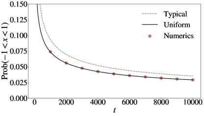
Figure 7: The probability of occupying the interval $-1<x<1$ for a resetting process to the origin $x=0$ versus time. Here we use the one sided Lévy distribution Eq. (53) to model the time intervals between resetting, so $\alpha=1/2$ which is the transition exponent. Simulations nicely match the uniform approximation Eq. (61) while the theory based on typical fluctuations Eq. (62) does not work so well. Here $D=1/2$ and for simulations we use $2\cdot 10^{7}$ trajectories.

VI.5 The transition case $\alpha=1/2$

Using $\alpha=1/2$ as an example and for the waiting time PDF Eq. (53) we have from Eq. (16) the survival probability $S(B)=\mbox{Erf}(1/\sqrt{2B})$, and $\langle\tau^{*}(t)\rangle=\sqrt{2\pi t}$, as mentioned. Therefore the uniform approximation reads

$$\rho_{{\rm Uni}}(x,t)=\int_{0}^{t}{\rm d}B{\mbox{Erf}\left({1\over\sqrt{2B}}\right)G(x,B)\over\sqrt{2\pi(t-B)}},$$ (59)

where we used $D=1/2$. This for large $x$ describes well the typical fluctuations given by the arcsine law for $B$

$$\rho_{{\rm Arcsine}}(x,t)=\int_{0}^{t}{\rm d}B{G(x,B)\over\pi\sqrt{B}\sqrt{t-B}},$$ (60)

which is the same as Eq. (19) for $\alpha=1/2$. This approximation diverges on the origin $x=0$ namely in the vicinity of the resetting point, while in reality and according to Eq. (59) such a behavior is not found. The two solutions are used in Fig. 6 where the numerics clearly demonstrates that the uniform approximation is the valid theory. The uniform solution and numerics exhibit a cusp in the density close to $x=0$.

Using Eq. (59) we obtain the probability of finding the particles in the interval $(-1,1)$. We use $\int_{-1}^{1}\exp[-x^{2}/(2B)]{\rm dx}/\sqrt{2\pi B}=\mbox{Erf}[1/\sqrt{2B}]$ to find

$$\mbox{Prob}_{\rm Uni}(-1<x<1)={1\over\sqrt{2\pi}}\int_{0}^{t}{\mbox{Erf}^{2}\left[{1\over\sqrt{2B}}\right]\over\sqrt{t-B}}{\rm d}B.$$ (61)

This integral is solved numerically and compared with Monte-Carlo simulations in Fig. 7 showing the validity of the uniform approximation. We compare this solution to the one obtained using the description of the typical fluctuations namely using the scaling function $g_{\alpha}(\xi)$ with $\alpha=1/2$. Recall that this solution does not depend explicitly on the waiting time PDF $\psi(\tau)$ besides $\alpha$ of course, unlike the uniform approximation. Using Eq. (23) and $D=1/2$

$$\mbox{Prob}_{{\rm typical}}(-1<x<1)\simeq$$

$$-\int_{-1}^{1}{\rm d}x{1\over\sqrt{2t}\pi^{3/2}}\left[2\ln|x|/\sqrt{t}-\gamma-3\ln 2\right]=$$

$${\sqrt{2}\over\sqrt{t\pi^{3}}}\left(\ln t+2+\gamma+3\ln 2\right).$$ (62)

This solution is plotted in Fig. 7 where its performance compared with the uniform approximations are shown to be weak. The $\ln(t)$ logarithmic behavior in (62) indicates the particularly slow nature of convergence to asymptotic results, strengthening the need for the uniform approximation at this transition case $\alpha=1/2$. We also integrated Eq. (60) in the interval $-1<x<1$ to estimate $\mbox{Prob}(-1<x<1)$. This solution works slightly better than the simple analytical expression Eq. (62) yet still not matching the uniform approximation Eq. (61). It is not plotted to avoid burdening the eye.

VI.6 Uniform Approximation: An Example

We now check the predictions of the uniform approximation using the Pareto distribution for waiting times and $\alpha=1/4$ so $\psi(\tau)=0.25\tau^{-5/4}$ for $\tau>1$, otherwise $\psi(\tau)=0$. In this case, from Eq. (6), $(\tau_{0})^{1/4}=1/4$ and using Eq. (13) $\langle\tau^{*}(t)\rangle=\sqrt{2}\pi t^{3/4}$. The survival probability is $S(B)=1$ if $B<1$ and $S(B)=B^{-1/4}$ for $1<B$ hence using Eq. (56) we have for $t>1$

$$\rho_{{\rm Uni}}(x,t)=\int_{0}^{1}{G(x,B){\rm d}B\over\sqrt{2}\pi(t-B)^{3/4}}+\int_{1}^{t}{G(x,B){\rm d}B\over\sqrt{2}\pi B^{1/4}(t-B)^{3/4}}.$$ (63)

This solution should be compared with the one obtained using the scaling solution Eq. (19)

$$\rho(x,t)\sim{1\over\sqrt{2}\pi}\int_{0}^{t}{G(x,B){\rm d}B\over(t-B)^{3/4}B^{1/4}}.$$ (64)

which is valid when $x$ and $t$ are large while $\xi=|x|/\sqrt{t}$ is finite and we set $D=1/2$. This gives according to Eq. (20) $\rho(x,t)\sim g_{1/4}(\xi)/\sqrt{t}$ where the scaling function $g_{1/4}(\xi)$ is presented in Eq. (22). Recall that from the infinite density Eq. (26) we have the approximation, valid for finite $x$ and large $t$

$$\rho(x,t)\sim{g_{1/4}(0)\over\sqrt{2Dt}}={\Gamma(1/4)\sqrt{t}\over\sqrt{2}\Gamma(3/4)\pi}\simeq{0.66593\over\sqrt{t}}.$$ (65)

In Fig. 8 we make the comparison between the various approximations. The figure shows that for finite time $t$, the uniform approximation works very well. Of course for the very long time limit the simulations results will converge to the theoretical prediction of the infinite density, which is given by the straight line in the Figure.

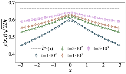
Figure 8: The infinite density versus $x$ for using the Pareto PDF for waiting times with $\alpha=1/4$ and $t_{0}=1$. In simulation we plot the histogram for the probability density $\rho(x,t)$ multiplied by $\sqrt{2Dt}$. In solid lines the uniform approximation Eq. (63) for intermediate times and in dashed lines the infinite density $\tilde{{\cal I}}^{\infty}(x)\simeq 0.6659$, Eq. (26). Here $D=1/2$ and we use $10^{8}$ trajectories.

We also find the probability that the particle is in the interval $-1<x<1$ at time $t$. Using $\int_{-1}^{1}G(x,B){\rm d}x=\mbox{Erf}[1/\sqrt{2B}]$ we have for the uniform approximation

$$\mbox{Prob}_{{\rm Uni}}(-1<x<1)=$$

$$\int_{0}^{1}{\mbox{Erf}\left[{1\over\sqrt{2B}}\right]{\rm d}B\over\sqrt{2}\pi(t-B)^{3/4}}+\int_{1}^{t}{\mbox{Erf}\left[{1\over\sqrt{2B}}\right]{\rm d}B\over\sqrt{2}\pi\left(t-B\right)^{3/4}B^{1/4}}.$$ (66)

These integrals can be numerically computed using programs like Mathematica or Maple. On the other hand from Eq. (65) we have

$$\mbox{Prob}(-1<x<1)\simeq 0.66592|\Delta x|/\sqrt{t}$$

where $|\Delta x|=2$ is the length of the interval $-1<x<1$ under study.

Fig. 9 clearly demonstrated the useful aspect of the uniform approximation as it captures the approach to the asymptotic limit, i.e. the straight line in the figure.

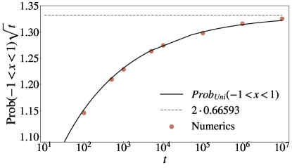
Figure 9: Probability of occupying the interval $-1<x<1$ times $\sqrt{t}$ as a function of time. The points belong to the data from Fig. 3 and Fig. 8 while the solid line represents the uniform approximation Eq. (66). Here the times between resets follow a Pareto PDF with $t_{0}=1$, $\alpha=1/4$. $D$ is $1/2$ and we use $10^{8}$ realizations.

VII Ergodic theory

So far we have studied useful approximation for the density of particles. We now study the ergodic properties of the process. Consider an observable, namely a functional of the stochastic path of the resetting process, ${\cal O}[x(t)]$ Meylahn2015 ; Hollander2019 . The time averages are denoted by

$$\overline{{\cal O}(t)}=\frac{1}{t}\int_{0}^{t}{\cal O}[x(t^{\prime})]{\rm d}t^{\prime}$$ (67)

while the ensemble average is $\langle{\cal O}(t)\rangle=\int_{-\infty}^{\infty}{\cal O}(x)\rho(x,t){\rm d}x$. For thin tailed PDFs of resetting times, time and ensemble averages are identical in the long time limit

$$\lim_{t\to\infty}\overline{{\cal O}(t)}=\langle{\cal O}\rangle^{{\rm ss}}$$ (68)

and

$$\langle{\cal O}\rangle^{{\rm ss}}=\int_{-\infty}^{\infty}{\cal O}(x)\rho^{{\rm ss}}(x){\rm d}x$$ (69)

where the normalized NESS density $\rho^{{\rm ss}}(x)$ is defined in Eq. (17). We did not prove this expected result, but some arguments why it is correct are given below. Note that in Eq. (69) we have assumed that the integral on the right hand side does not diverge, namely that the observable ${\cal O}(x)$ is integrable with respect to the normalized steady state. So far in this section $\langle\tau\rangle$ was finite, what is the ergodic theory when this mean time diverges?

For fat tailed resetting times, with $0<\alpha<1$ infinite ergodic theory holds. This means that the non-normalized steady state will play a special role in the evaluation of the time averages. First consider the ensemble averages, in the long time limit we find two types of behaviors. For $1/2<\alpha<1$ using Eq. (18)

$$\langle{\cal O}(t)\rangle=\int_{-\infty}^{\infty}{\cal O}(x)\rho(x,t){\rm d}x\sim{\int_{-\infty}^{\infty}{\cal O}(x)\tilde{{\cal I}}^{\infty}(x){\rm d}x\over\langle\tau^{*}(t)\rangle}.$$ (70)

where we use Eq. (18), so $\rho(x,t)\sim\tilde{{\cal I}}^{\infty}(x)/\langle\tau^{*}(t)\rangle$. Similarly using Eq. (26) for $0<\alpha<1/2$

$$\langle{\cal O}(t)\rangle\sim{\int_{-\infty}^{\infty}{\cal O}(x)\tilde{{\cal I}}^{\infty}(x){\rm d}x\over\sqrt{2Dt}}.$$ (71)

We assumed that the integrals do not diverge, namely that the observable is integrable with respect to the infinite invariant density $\tilde{{\cal I}}^{\infty}(x)$. Eqs. (70,71) show that while $\tilde{{\cal I}}^{\infty}(x)$ is not normalized, it is used to obtain ensemble averages. More precisely

$$\begin{array}[]{l l}\lim_{t\to\infty}\langle\tau^{*}(t)\rangle\langle{\cal O}(t)\rangle=\int_{-\infty}^{\infty}{\cal O}(x)\tilde{{\cal I}}^{\infty}(x){\rm d}x&\mbox{if}\ 1/2<\alpha<1\\ &\\ \lim_{t\to\infty}\sqrt{2Dt}\langle{\cal O}(t)\rangle=\int_{-\infty}^{\infty}{\cal O}(x)\tilde{{\cal I}}^{\infty}(x){\rm d}x&\mbox{if}\ 0<\alpha<1/2,\end{array}$$ (72)

thus $\langle\tau^{*}(t)\rangle$ and $\sqrt{2Dt}$ replace normalizing factors.

An example for an integrable observable consider

$${\cal O}[x(t)]=\theta(a<x(t)<b)$$ (73)

where $\theta(a<x(t)<b)$ is the pulse function, namely it is equal unity if the condition in the parentheses holds, otherwise it is zero. Since the integral $\int_{a}^{b}\tilde{{\cal I}}^{\infty}(x){\rm d}x$ is finite, for finite $a$ and $b$, the observable is called integrable, we will now use this observable to discuss time averages.

VII.1 Example

As an example consider the case $\alpha=3/4$ with the Pareto PDF discussed in subsection IV.5 with $D=1/2$. The observable of interest is the pulse function $\theta(-3<x(t)<3)$. Using the infinite density Eq. (31)

$$\langle\tau^{*}(t)\rangle\langle\theta(-3<x(t)<3)\rangle\sim\int_{-3}^{3}\tilde{{\cal I}}^{\infty}_{\alpha=3/4}(x){\rm d}x.$$ (74)

The integral is solved numerically and we find

$$\lim_{t\to\infty}\langle\tau^{*}(t)\rangle\langle\theta(-3<x(t)<3)\rangle=8.91711\cdots$$ (75)

and $\langle\tau^{*}(t)\rangle$ is given in Eq. (27) with $\alpha=3/4$. As mentioned $\langle\theta(-3<x(t)<3)\rangle$ is the probability that a member of an ensemble of particles occupies the domain $[-3,3]$ at time $t$. This prediction is tested in Fig. 10 showing that the non-normalized invariant density is the tool of choice to compute ensemble averages of integrable observables.

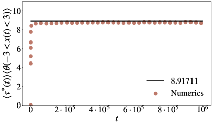
Figure 10: Time evolution of $\langle\theta(-3<x(t)<3)\rangle$ times $\langle\tau^{*}(t)\rangle$ Eq. (27) for a Pareto PDF with $\alpha=3/4$ and $t_{0}=1$. The solid line represents the long time limit Eq. (75). Here $D=1/2$ and we have used $10^{6}$ trajectories.

VII.2 Time averages

The time integration over the pulse function observable Eq. (73) is the total time a trajectory $x(t^{\prime})$ spends in the domain $[a,b]$ during the measurement time interval $(0,t)$, it will be denoted $\tilde{T}$. For example $[a,b]$ can be a domain in space including the resetting point, or not. The total time the particle spends in $[a,b]$ is called the occupation time or the residence time Pal2019 ; Bressloff2020 ; Singh2022 . For thin tailed distributions of resetting times, and using the ergodic hypothesis

$$\lim_{t\to\infty}{\int_{0}^{t}\theta(a<x(t^{\prime})<b){\rm d}t^{\prime}\over t}=\int_{a}^{b}\rho^{{\rm ss}}(x){\rm d}x$$ (76)

which is the probability a member of an ensemble of particles in NESS occupies the domain. We will treat this observable for the case $\alpha<1$ below.

We now treat an integrable observable not restricting our selves to an example. Then the ensemble averaged time average

$$\langle\overline{{\cal O}}(t)\rangle\sim{1\over t}\left\langle\int_{0}^{t}{\cal O}(t^{\prime}){\rm d}t^{\prime}\right\rangle$$ (77)

which is found by averaging many of the underlying processes, over time and over independent trajectories. Since the ensemble average in any experiment is simply a sum over a finite sample, we may replace the order of time and ensemble average and then

$$\langle\overline{{\cal O}}(t)\rangle={\int_{0}^{t}\left[\int_{-\infty}^{\infty}\rho(x,t^{\prime}){\cal O}(x){\rm d}x\right]{\rm d}t^{\prime}\over t}.$$ (78)

As before, in the long time limit we replace the density $\rho(x,t)$ with the infinite density using Eq. (18) , e.g. for $1/2<\alpha<1$

$$\langle\overline{{\cal O}}(t)\rangle\sim{\int_{0}^{t}\left[\int_{-\infty}^{\infty}{\tilde{{\cal I}}^{\infty}(x)\over\langle\tau^{*}(t^{\prime})\rangle}{\cal O}(x){\rm d}x\right]{\rm d}t^{\prime}\over t}.$$ (79)

In the numerator we can identify the ensemble average obtained with integration over the infinite density Eq. (70). Further the time integration is straight forward, using Eqs. (70,71) we find

$$\lim_{t\to\infty}{\langle\overline{{\cal O}}(t)\rangle\over\langle{\cal O}(t)\rangle}=\left\{\begin{array}[]{c c}1&\ \mbox{for}\ \psi(\tau)\ \mbox{thin tailed}\\ &\\ {1\over\alpha}&\ {1\over 2}<\alpha<1\\ &\\ 2&\ 0<\alpha<{1\over 2}.\end{array}\right.$$ (80)

We see that the time and ensemble averages are related one to another. For $\alpha<1$ they are calculated using the infinite density other wise by the normalized invariant density of the NESS. The prefactors found for $\alpha<1$ stem from simple time integration. We see that when $\alpha=1$ and $\alpha=1/2$ there is an ergodic transition in the system which is in principle easy to detect when $\alpha$ is tuned (the result in the first line, holds for any distribution, of resetting times, even a distribution that decays like a power law $\alpha>1$, in such a way that the mean resetting time is finite). The predictions in Eq. (80) are tested with finite time simulations, showing excellent agreement without fitting.

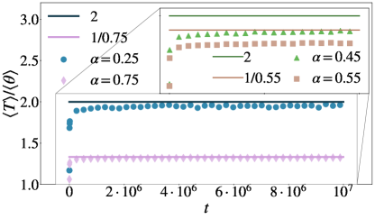
Figure 11: Ratio between the ensemble-averaged time average and the ensemble average versus time. The observable is the pulse function Eq. (73) in the interval $-10<x<10$ . We present numerical results for the Pareto reset time PDF with $t_{0}=1$ with $\alpha=1/4$ and $\alpha=3/4$. In solid lines the long time limit of $\langle T\rangle/\langle\theta\rangle$, Eq. (80). In the inset figure, we present the same results but for $\alpha$ near the transition point below, $\alpha=0.45$ and above $\alpha=0.55$. We can see that the agreement is not so good due to the slowing down of the convergence near the transition in agreement with what is observed also in Fig. 12. Here $D=1/2$ and we have used $10^{7}$ trajectories.

Infinite ergodic theory deals also with the limiting laws of the distribution of time averages. We define a dimensionless variable

$$\eta={\overline{{\cal O}}\over\langle\overline{{\cal O}}\rangle}$$ (81)

and clearly the mean of $\eta$ is unity. In what follows assume that the observable is integrable, namely the non-zero denominator is obtained in theory from the invariant density using Eqs. (70,71,80) though a direct measurement in say an experiment or simulation is also a good possibility. For thin tailed waiting time PDFs, $\eta$ in the long time limit is not fluctuating. In other words its distribution is a delta function centred on unity.

VII.3 Fluctuations of time averages

Consider the integral over the pulse function Eq. (73)

$$\eta={\int_{0}^{t}\theta(-a<x(t)<a){\rm d}t\over\langle\int_{0}^{t}\theta(-a<x(t)<a){\rm d}t\rangle}={\tilde{T}\over\langle\tilde{T}\rangle}.$$ (82)

Namely we are interested in the statistics of the occupation time $\tilde{T}$ in $[-a,a]$ when the observation is in $(0,t)$. Of course the interval $[-a,a]$ contains the resetting point $x=0$. In Eq. (82) $\eta$ is normalized in the sense that its mean is unity.

The function $\theta(-a<x(t)<a)$ attains the value $1$ when $x(t)$ is in the domain $[-a,a]$, $0$ other wise. The observable is switching at random times between values $1$ and $0$, namely it is performing a dichotomous two state process. What is the physical mechanism of the return into the domain $[-a,a]$? One option is that the resetting returns the particle to the domain, namely just before a resetting event the particle is say on $x(t)>a$ and it is injected back to $-a<x=0<a$. Yet another option is that the particle, via the process of diffusion alone, returns back into the domain. We have here a competition between these two mechanisms of return. Recall that the PDF of resetting times is given by a fat tailed law Eq. (6) while the PDF of first passage time of BM in an infinite domain in dimension one decays like $(\mbox{time})^{-3/2}$ Redner , in the absence of resetting. Hence we might expect a transition in the ergodic properties of the system when $\alpha=1/2$, which is also noticed in the behavior of the infinite invariant densities discussed above.

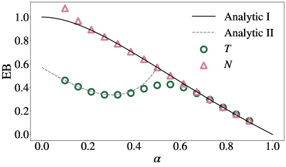
Figure 12: The EB parameter, describing the fluctuations of the time averages, versus $\alpha$. Numerical results for the occupation time $T$, for the reset process are presented, where we used $D=1/2,a=0.1$ the Pareto reset time PDF, with $t_{0}=1$. For $1/2<\alpha<1$, the EB parameter is the same as that for $N$ (triangles), the number of resets up to time $t$. Close to the transition point $\alpha=1/2$ we see deviations from theory, due to finite sampling and slowing down of the convergence. When $0<\alpha<1/2$ the fluctuations are non-trivial and we observe a minimum for the EB parameter. Here we have used $10^{5}$ trajectories evolved since $t=10^{10}$. We used Eq. (84) (Analytic II) and Eq. (85) (Analytic I) to present the theory.

To quantify this behavior we use the EB parameter He2008 , defined as

$$\mbox{EB}={\langle\eta^{2}\rangle-\langle\eta\rangle^{2}\over\langle\eta\rangle^{2}}={\langle\tilde{T}^{2}\rangle-\langle\tilde{T}\rangle^{2}\over\langle\tilde{T}\rangle^{2}}.$$ (83)

An analysis of the EB parameter starts in the next section and more details are found in Appendix B and C. In the long time limit

$$\textrm{EB}=\left\{\begin{array}[]{cc}\alpha\pi-1+\frac{1}{2}\left[\frac{\pi\Gamma\left(1-\alpha\right)}{\Gamma\left(\frac{1}{2}-\alpha\right)}\right]^{2},&0<\alpha<1/2\\ &\\ \frac{2\Gamma^{2}(1+\alpha)}{\Gamma(1+2\alpha)}-1,&1/2<\alpha<1\\ &\\ 0,&\mbox{thin tailed PDFs}\end{array}\right.$$ (84)

When the mean of the resetting time PDF is finite there is no ergodicity breaking as the PDF of $\eta$ converges to a delta function and $\rm{EB}=0$. In contrast if $0<\alpha<1$ we have two types of behaviors. Note that when $\alpha\to 0$, we have $\mbox{EB}=(\pi/2)-1\simeq 0.57$. As shown below, just after Eq. (90) this is the value of the EB parameter for free BM (see also Appendix B).

When $1/2<\alpha<1$ the fluctuations we find are related to the fluctuations of the number of resets in the time interval $(0,t)$. More specifically recall that $N$ is the random number of resets in the time interval $(0,t)$. The EB parameter for this observable is well known He2008

$${\rm EB}={\langle N^{2}\rangle-\langle N\rangle^{2}\over\langle N\rangle^{2}}=\frac{2\Gamma^{2}(1+\alpha)}{\Gamma(1+2\alpha)}-1,$$ (85)

which is valid for $0<\alpha<1$ and in the long time limit. We see that the fluctuations of the time averages are related to the fluctuations of the number of resettings, however this is true only when $1/2<\alpha<1$. The intuitive explanations is that when $1/2<\alpha$ the return to the domain $[-a,a]$ is dominated by resetting and not by diffusion. Further the time spent in side the domain $[-a,a]$ is statistically short compared to the time outside the domain, and hence it is the fluctuations of the latter that dominate the statistics of the time averages. The same is not true for thin tailed PDFs where the mean times in and out side of the domain are both finite. Hence in the latter case we find ordinary ergodicity.

To summarize, one can say that for $0<\alpha<1/2$ the fluctuations are less trivial if compared to other cases. As mentioned more technical details are provided below. In Fig. 12 we present numerical results for the EB parameter. We observe a minimum for the EB parameter found also in the context of a study of laser cooling Barkai2021 . The convergence of finite time simulations is poor close to the critical value of $\alpha=1/2$, an effect that could be studied further.

VIII Occupation time statistics

As mentioned, we call the time spent by the resetting process $x(t^{\prime})$ in the spatial domain $[-a,a]$, within the time window $(0,t)$, $\tilde{T}$, where the resetting is to the origin $x=0$. The PDF of this random variable will be denoted $P(\tilde{T},t)$. For standard ergodic processes, and in the limit of long times, we expect that this PDF becomes a narrow distribution, centred around the mean, as mentioned already. However, when $\alpha<1$ this is not true any more. To analyze this issue, we use a tool developed by Montroll, Weiss and others in the context of continuous time random walks Klafter . The same tool was used to study ergodic properties of sub-recoil laser cooled gases Barkai2021 . Here the first goal is to relate between statistics of occupation times of Brownian motion and those of the occupation times of the reseted process. Secondly, we derive the basic formulas of infinite ergodic theory from a well known approach, and further provide simple intuitive formulas for averages. We start with a recap of occupation time statistics for Brownian motion.

VIII.1 Occupation time for Brownian motion

Consider reset free Brownian motion $x_{{\rm BM}}(t)$ starting on the origin $x=0$. The occupation time of the process is

$$T_{{\rm BM}}(t)=\int_{0}^{t}\theta[x_{{\rm BM}}(t^{\prime})]{\rm d}t^{\prime}$$ (86)

Here and in what follows we use $\theta[x_{{\rm BM}}(t)]=\theta(-a<x_{{\rm BM}}(t)<a)$ as a short hand notation. The mean of the pulse function is obtained from the Gaussian packet

$$\langle\theta[x_{{\rm BM}}(t)]\rangle=\int_{-\infty}^{\infty}G(x,t)\theta[x]{\rm d}x.$$ (87)

Hence the mean occupation time is $\langle T(t)\rangle_{{\rm BM}}=\int_{0}^{t}\langle\theta[x_{{\rm BM}}(t^{\prime})]\rangle{\rm d}t^{\prime}$ and using Eq. (1) it is easy to show that

$$\langle T(t)\rangle_{{\rm BM}}=t+{a\sqrt{t}\over\sqrt{\pi D}}\exp\left(-{a^{2}\over 4Dt}\right)-\left(t+{a^{2}\over 2D}\right)\mbox{Erfc}\left({a\over\sqrt{4Dt}}\right).$$ (88)

In the long time limit

$$\langle T(t)\rangle_{{\rm BM}}\sim{2a\over\sqrt{\pi D}}t^{1/2}.$$ (89)

The distribution of the occupation time of Brownian motion is discussed further in Appendix B. Using the Feynmann-Kac formalism Kac ; Functionals , the PDF of the occupation time in the long time limit is half a Gaussian

$$\mbox{PDF}_{{\rm BM}}(T|t)\sim\left({D\over\pi a^{2}t}\right)^{1/2}\exp\left(-{DT^{2}\over 4a^{2}t}\right).$$ (90)

The Laplace transform of the finite time solution is presented in Appendix B. The long time limit of the EB parameter is $\mbox{EB}=(\langle T^{2}\rangle_{{\rm BM}}-\langle T\rangle_{{\rm BM}}^{2})/\langle T\rangle_{{\rm BM}}^{2}=(\pi/2)-1$, namely the same as the reseted process Eq. (84) when $\alpha\to 0$.

VIII.2 Occupation time for the resetting problem

The occupation time of the reseted process $\tilde{T}(t)=\int_{0}^{t}\theta[x(t^{\prime})]{\rm d}t^{\prime}$ is now considered. With the notation for time averages Eq. (67) and for the pulse function observable $\overline{{\cal O}}=\tilde{T}/t$. Let $Q_{N}(\tilde{T},t){\rm d}t{\rm d}\tilde{T}$ be the probability that the $N$th resetting event takes place in the time interval $(t,t+{\rm d}t)$ when the value of the occupation time is within $(\tilde{T},\tilde{T}+{\rm d}\tilde{T})$. This function is given by the iteration rule

$$Q_{N+1}(\tilde{T},t)=\int_{0}^{\tilde{T}}{\rm d}T^{\prime}\int_{0}^{t}{\rm d}\tau Q_{N}\left(\tilde{T}-T^{\prime},t-\tau\right)\phi(T^{\prime},\tau).$$ (91)

Here $\phi(T^{\prime},\tau)$ is the joint PDF of the resetting interval $\tau$ i.e. the time between consecutive resets, and the occupation time in the same interval $T^{\prime}$. According to Eq. (3) the resetting process is defined with a sequence of time intervals between resettings

$$\left\{\tau_{1},\tau_{2},...\tau_{N},B\right\}.$$

Within each resetting interval $\tau_{i}$ we have an occupation time $T_{i}$ in the spatial domain $(-a,a)$. Given the reset time interval $\tau_{i}$, statistical properties of $T_{i}$ are determined by the laws of Brownian motion. Clearly the occupation time for the reseted process is

$$\tilde{T}=\sum_{i=1}^{N}T_{i}+T_{B}.$$ (92)

$T_{B}$ is the occupation time in the interval $(-a,a)$ gained in the backward time $B$. The sets $\{T_{i}\}$ and $\{\tau_{i}\}$ are separately composed from IID random variables, however $T_{i}$ and $\tau_{i}$ are mutually dependent. The longer is $\tau_{i}$ the longer $T_{i}$ is, in statistical sense. The joint PDF of the pair is

$$\phi(T,\tau)=\psi(\tau)\mbox{PDF}_{{\rm BM}}(T|\tau).$$ (93)

Where here we use the PDF of occupations times for Brownian motion without restarts.

Eq. (91) describes the basic property of the process. To arrive in $\tilde{T}$ at time $t$ when the previous resetting took place at $t-\tau$, the previous value of $\tilde{T}$, at the moment of the previous reseting, was $\tilde{T}-T$. Notice that in Eq. (91) time $t$ denotes a dot on the time axis, on which a resetting took place (see details below). Solving Eq. (91) is possible with the help of the convolution theorem of Laplace transform. Let

$$\hat{Q}_{N}(p,s)=\int_{0}^{\infty}{\rm d}\tilde{T}\int_{0}^{\infty}{\rm d}t\exp\left(-p\tilde{T}-st\right)Q_{N}(\tilde{T},t)$$ (94)

be the double Laplace transform of $Q_{N}(\tilde{T},t)$ where $p\leftrightarrow\tilde{T}$ and $s\leftrightarrow t$ are Laplace pairs. The convolution theorem and the iteration rule give $\hat{Q}_{N+1}(p,s)=\hat{Q}_{N}(p,s)\hat{\phi}(p,s)$ where $\hat{\phi}(p,s)$ is the double Laplace transform of $\phi(T,\tau)$. Using the seed, $Q_{0}(\tilde{T},t)=\delta(\tilde{T})\delta(t)$, reflecting the initial condition, namely that the resetting process starts at time $t=0$, we have

$$\hat{Q}_{N}(p,s)=\left[\hat{\phi}(p,s)\right]^{N}.$$ (95)

The PDF $P(\tilde{T},t)$ is in turn given by

$$P(\tilde{T},t)=\sum_{N=0}^{\infty}\int_{0}^{\tilde{T}}{\rm d}T^{{}^{\prime}}_{B}\int_{0}^{t}{\rm d}BQ_{N}\left(\tilde{T}-T^{{}^{\prime}}_{B},t-B\right)\Phi(T_{B},B).$$ (96)

Here we summed over the number of restarts $N$ and took into consideration the fact that the observation time $t$, is found at a time $B$ after the last resetting event in the sequence. We further integrate over the backward recurrence time. Finally, the statistical weight function is

$$\Phi(T_{B},B)=S(B)\mbox{PDF}_{{\rm BM}}(T_{B}|B)$$ (97)

where as before $S(B)=\int_{B}^{\infty}\psi(\tau){\rm d}\tau$ is the survival probability, i.e. the probability of not resetting. We will soon use the Laplace $B\to s$ transform of this function $\hat{S}(s)=[1-\hat{\psi}(s)]/s$ where $\hat{\psi}(s)$ is the Laplace transform of $\psi(\tau)$.

Now we again use the convolution theorem. Let $\hat{P}(p,s)$ be the double Laplace transform of $P(\tilde{T},t)$. Using Eq. (96)

$$\hat{P}(p,s)=\sum_{N=0}^{\infty}\hat{Q}_{N}(p,s)\hat{\Phi}(p,s)$$ (98)

where

$$\hat{\Phi}(p,s)=\int_{0}^{\infty}\int_{0}^{\infty}\exp[-T_{B}p-Bs]S(B)\mbox{PDF}_{{\rm BM}}(T_{B}|B){\rm d}T_{B}{\rm d}B.$$ (99)

Inserting Eq. (95) Eq. (98) and summing the geometric series

$$\hat{P}(p,s)={\hat{\Phi}(p,s)\over 1-\hat{\phi}(p,s)}.$$ (100)

In the context of continuous time random walks such an equation is used to analyse the positional PDF of the packet of particles, though then usually one invokes a Fourier-Laplace transform Klafter ; Fifty ; Sergey ; Aghion . The inversion of the formal solution Eq. (100) to the $(\tilde{T},t)$ domain is a significant problem, which can be tackled analytically in the long time limit. In particular from the definition of the Laplace transform

$$\hat{P}(p,s)=\int_{0}^{\infty}{\rm d}\tilde{T}\int_{0}^{\infty}{\rm d}t\exp[-p\tilde{T}-st]P\left(\tilde{T},t\right)=$$

$$\int_{0}^{\infty}(1-p\tilde{T}+\cdots){\rm d}\tilde{T}\int_{0}^{\infty}{\rm d}te^{-st}P(\tilde{T},t)$$

$$={1\over s}-p\langle\tilde{T}(s)\rangle\cdots$$

where we used the normalization condition for $P(\tilde{T},t)$ and $\langle\hat{\tilde{T}}(s)\rangle$ is the Laplace $t\to s$ transform of the mean occupation time $\langle\tilde{T}(t)\rangle$. Another way to write this is

$$\langle\hat{\tilde{T}}(s)\rangle=-{\partial\hat{P}(p,s)\over\partial p}|_{p=0}.$$ (101)

Using the Montroll-Weiss like equation (100) we find

$$\langle\hat{\tilde{T}}(s)\rangle=-{\partial_{p}\hat{\Phi}(p,s)|_{p=0}\over 1-\hat{\phi}(p=0,s)}-{\partial_{p}\phi(p,s)|_{p=0}\hat{\Phi}(p=0,s)\over[1-\phi(p=0,s)]^{2}}.$$ (102)

Similar approach can be used to find the variance of the occupation time, however here will will study the mean only.

We use $\hat{\phi}(p=0,s)=\hat{\psi}(s)$, $\hat{\Phi}(p=0,s)=[1-\hat{\psi}(s)]/s$, and

$$\partial_{p}\hat{\phi}(p,s)|_{p=0}=-\int_{0}^{\infty}\exp(-s\tau)\langle T(\tau)\rangle_{{\rm BM}}\psi(\tau){\rm d}\tau$$ (103)

where

$$\langle T(\tau)\rangle_{{\rm BM}}=\int_{0}^{\infty}T\cdot\mbox{PDF}_{{\rm BM}}(T|\tau){\rm d}T$$ (104)

is the mean occupation time of a Brownian motion in $(-a,a)$, in the time interval $(0,\tau)$. Similarly

$$\partial_{p}\hat{\Phi}(p,s)|_{p=0}=-\int_{0}^{\infty}\exp(-sB)\langle T(B)\rangle_{{\rm BM}}S(B){\rm d}B.$$ (105)

Using Eq. (103) we find

$$\langle\hat{\tilde{T}}(s)\rangle=\underbrace{{\int_{0}^{\infty}\langle T(\tau)\rangle_{{\rm BM}}\psi(\tau)e^{-s\tau}{\rm d}\tau\over s\left[1-\hat{\psi}(s)\right]}}_{{\cal T}_{1}(s)}+\underbrace{{\int_{0}^{\infty}\langle T(B)\rangle_{{\rm BM}}S(B)e^{-sB}{\rm d}B\over 1-\hat{\psi}(s)}}_{{\cal T}_{2}(s)}.$$ (106)

This formula relates between the mean occupation time of the resetting process, with the mean occupation time of the restart free Brownian motion, and with the waiting time $\psi(\tau)$. We note that Eq. (106) can be generalized to other observables beyond the occupation time. The two contributions defined in this equation, namely ${\cal T}_{1}(s)$ and ${\cal T}_{2}(s)$, describe contributions to the occupation time before and after the last reset event in the sequence.

VIII.2.1 Mean occupation time $1/2<\alpha<1$

To analyze the long time behavior of the mean occupation time we consider the small $s$ limit, following a standard approach by considering Eq. (46) which holds for $0<\alpha<1$. We now need to distinguish between three cases. A short calculation, valid when $1/2<\alpha<1$ will convince the reader that the leading term, when $s\to 0$ in Eq. (106) reads

$$\langle\hat{\tilde{T}}(s)\rangle\sim{\int_{0}^{\infty}\langle T(\tau)\rangle_{{\rm BM}}\psi(\tau){\rm d}\tau\over b_{\alpha}s^{1+\alpha}},$$ (107)

and only ${\cal T}_{1}(s)$ is contributing to this limit. Inverting to the time domain we find in the long time limit

$$\langle\tilde{T}(t)\rangle\sim{t^{\alpha}\over\Gamma(1+\alpha)b_{\alpha}}\int_{0}^{\infty}\langle T(\tau)\rangle_{{\rm BM}}\psi(\tau){\rm d}\tau.$$ (108)

Noticing that the average number of restarts is $\langle N(t)\rangle_{{\rm Res}}\sim t^{\alpha}/b_{\alpha}\Gamma(1+\alpha)$ we have

$$\langle\tilde{T}(t)\rangle\sim\langle N(t)\rangle_{{\rm Res}}\langle\langle T\rangle_{{\rm BM}}\rangle_{{\rm Res}}$$ (109)

where the mean of the occupation time, within a resetting period, averaged over the resetting time is

$$\langle\langle T\rangle_{{\rm BM}}\rangle_{{\rm Res}}=\int_{0}^{\infty}\int_{0}^{\infty}T\cdot\mbox{PDF}_{{\rm BM}}(T|\tau){\rm d}T\psi(\tau){\rm d}\tau.$$ (110)

In Eqs. (109,110) we distinguish between averages over the reseting time, and the averages over the Brownian motion within each interval. Eq. (109) is expected, a main point to notice is that it is not valid when $0<\alpha<1/2$. Since $\langle T(\tau)\rangle_{{\rm BM}}\sim\tau^{1/2}$, when averaging over $\psi(\tau)\propto\tau^{-1-\alpha}$, the integral in Eq. (110) diverges when $\alpha<1/2$, a case soon to be treated.

Eq. (109) remains valid for the case where the mean of the waiting time between resets is finite, for example when $\psi(\tau)$ is an exponential function. The difference is that $\langle N(t)\rangle_{{\rm Res}}\sim t/\langle\tau\rangle$, where $\langle\tau\rangle$ is the mean time between restarts.

How is Eq. (108) related to the non-normalised invariant density when $1/2<\alpha<1$? Using the pulse function Eq. (73) of a Brownian path without resetting

$$\langle T(\tau)\rangle_{{\rm BM}}=\left\langle\int_{0}^{\tau}\theta[x(t^{\prime})]{\rm d}t^{\prime}\right\rangle_{{\rm BM}}=\int_{0}^{\tau}\langle\theta[x(t^{\prime})]\rangle{\rm d}t^{\prime}=\int_{0}^{\tau}\int_{-\infty}^{\infty}\theta[x]G(x,t^{\prime}){\rm d}x{\rm d}t^{\prime}$$ (111)

as mentioned already. Using Eq. (109) the occupation time for the resetting process is

$$\langle\tilde{T}(t)\rangle\sim\langle N(t)\rangle_{{\rm Res}}\int_{0}^{\infty}{\rm d}\tau\int_{-\infty}^{\infty}{\rm d}xG(x,\tau)\theta(x)[-\partial_{\tau}S((\tau)]$$ (112)

where we apply $\psi(\tau)=-\partial_{\tau}S(\tau)$. Integrating by parts, and employing Eq. (18)

$$\langle\tilde{T}(t)\rangle\sim\langle N(t)\rangle_{{\rm Res}}\int_{-\infty}^{\infty}\theta(x){\cal I}^{\infty}(x){\rm d}x.$$ (113)

which for the observable of interest, namely the pulse function reads $\langle\tilde{T}(t)\rangle\sim\langle N(t)\rangle_{{\rm Res}}\int_{-a}^{a}{\cal I}^{\infty}(x){\rm d}x$. By definition $\langle\tilde{T}(t)\rangle/t=\langle\overline{\theta}[x(t)]\rangle$ and hence the CTRW approach and Eq. (113) yield the same result as in Eq. (80) utilizing Eqs. (14, 70) and the long time identity $\partial_{t}\langle N(t)\rangle_{{\rm Res}}/\alpha=\langle N(t)\rangle_{{\rm Res}}/t$.

VIII.2.2 Mean occupation time $0<\alpha<1/2$

We now analyse the case $0<\alpha<1/2$. Here contributions to the mean occupation time stem from both terms in Eq. (106), namely now the backward recurrence time is large in statistical sense, in a way that it contributes to the averaged observable also in the long time limit. In the small $s$ limit, we use the asymptotic formula Eq. (89) and find employing Eq. (106) and $1-\hat{\psi}(s)\sim b_{\alpha}s^{\alpha}$

$${\cal T}_{1}(s)\sim{2a\over\sqrt{\pi D}}{\int_{0}^{\infty}\tau^{1/2}(\tau_{0})^{\alpha}\tau^{-1-\alpha}\exp(-s\tau){\rm d}\tau\over b_{\alpha}s^{1+\alpha}},$$ (114)

where we used Eq. (6). Inserting the definition of $b_{\alpha}$ given in Eq. (46) and integrating we find for small $s$

$${\cal T}_{1}(s)\sim{2\alpha a\over\Gamma(1-\alpha)\sqrt{\pi D}}\Gamma\left(1/2-\alpha\right)s^{-3/2}.$$ (115)

Inverting to the time domain we find

$${\cal T}_{1}(t)\sim{4a\over\pi\sqrt{D}}{\Gamma(1/2-\alpha)\over|\Gamma(-\alpha)|}t^{1/2}$$ (116)

The second contribution is analysed similarly, in particular employing Eq. (89)

$${\cal T}_{2}(s)\sim{2a\over\sqrt{\pi D}}{\int_{0}^{\infty}\sqrt{B}S(B)\exp(-sB){\rm d}B\over b_{\alpha}s^{\alpha}}.$$ (117)

Using $S(B)\sim(\tau_{0})^{\alpha}\tau^{-\alpha}/\alpha$ obtained from Eq. (6), integrating and then inverting to the time domain we find

$${\cal T}_{2}(t)\sim{4a\over\pi\sqrt{D}}{\Gamma(3/2-\alpha)\over\Gamma(1-\alpha)}t^{1/2}$$ (118)

Summing Eqs. (116, 118) we get the mean occupation time

$$\langle\tilde{T}(t)\rangle\sim{2a\over\pi\sqrt{D}}{\Gamma({1/2-\alpha})\over\Gamma(1-\alpha)}t^{1/2}.$$ (119)

When $\alpha\to 0$ we obtain the same result as found for Brownian motion, Eq. (89), while in the limit $\alpha\to 1/2$ this expression diverges signalling the transition.

The same result can be obtained from the infinite density approach. Since the occupation time is the time integral of the pulse function

$${\langle\tilde{T}(t)\rangle\over t}\sim 2\langle\theta(x)\rangle$$ (120)

where we used Eq. (80) which gives the prefactor $2$. The average $\langle\theta(x)\rangle$ is with respect to the infinite invariant density as in Eq. (71)

$$\langle\theta(x)\rangle\sim{\int_{-\infty}^{\infty}\theta(x){\cal I}^{\infty}(x){\rm d}x\over\sqrt{2Dt}}$$ (121)

As mentioned in Eq. (26) the infinite density is a constant in this case. It is then easy to show that the results obtained with CTRW approach are the same as those found with the infinite density method. Of course this is what is expected, though here once we have the infinite density, the calculation is straight forward, as is the case of ergodic processes, where time integration is replaced with a phase space integration. In Appendix B we continue with this line of study and calculate the fluctuations of the time averages, these are needed to obtain the $\rm{EB}$ parameter.

IX Discussion

Relating the NESS to the limiting laws of the backward recurrence times Godreche2001 ; Dynkin1955 ; Wanli2018 was our starting point. This is a valuable tool for many restart models, where the reset erases the memory of the process, and is not limited to BM. As studied in Bordova2019A the erasure of memory, which is clearly valid for a Markovian BM, is not the general rule. Using statistics of the backward recurrence time we simplified main expressions for NESS (that previously relied on Laplace transforms) and obtained results which were found previously with other methods Pal2016 ; Gupta2016 ; Eule2016 . We also added new ingredients to the resetting literature.

The tools of infinite ergodic theory, and the non-normalised NESS are employed to obtain general ergodic aspects of the restart process. The invariant densities can be normalised or non-normalised, still their functional dependence on the survival probability appears similar. Thus controlling the distribution of resetting time, we can explore either the standard ergodic phase, or the theory of infinite ergodic theory. The time scale $\langle\tau^{*}(t)\rangle$ and the length scale $\sqrt{2Dt}$ are used to relate the infinite density $\tilde{{\cal I}}^{\infty}(x)$ with the probability density $\rho(x,t)$, for $1/2<\alpha<1$ and $0<\alpha<1/2$ respectively. See Eqs. (18,26).

The behaviors of both time and ensemble averages were addressed. When dealing with thin tailed distributions the standard ergodic picture emerges. The exception is sharp restart, which has no NESS. The case of sporadic resetting with fat tailed distributed resetting times, was the main focus of this study. A statistical theory of the time averages works as follows. When $\alpha<1$ we first check that the observable is integrable with respect to the non-normalized state. In this case we find the ensemble average using the infinite invariant density. Once this is known, we use Eq. (80) to obtain the ensemble average of the time average $\langle\overline{{\cal O}}\rangle$. We then studied the fluctuations of the time averages, focusing on an integrable observable, namely the pulse function. The time integral of this observable is the total time spent in an interval, called the occupation time. The fluctuations exhibited non-trivial effects, and a transition in the EB parameter was found for $\alpha=1/2$. Additionaly $\alpha=1/2$ marks a transition in the structure of the infinite invariant density itself. We further pointed out that when $1/2<\alpha<1$ the EB parameter of the time average, is the same as the one computed for the fluctuations of the number of renewals. This implies that the fluctuations in this phase are universal, and independent of the observable, as long as it is integrable, however we did not prove this statement. In contrast, when $0<\alpha<1/2$ the fluctuations of time averages, and the EB parameter, depend on the observable and hence non-universal.

We speculate that this type of transition is generic, and can be found similarly in other processes. As we showed, in our case, the transition is found when $\alpha$ matches the exponent describing the PDF of first passage times of a Brownian motion on a line in the absence of resetting. The latter well known PDF, with absorption at say $x=0$, decays like $(\mbox{first passage time})^{-(1+\beta)}$ and $\beta=1/2$ in dimension one. In many other processes $\beta\neq 1/2$, for example for diffusion in a potential that grows like the log of the distance, or for sub-diffusive CTRW, or random walks on some fractals or comb structures etc. We believe that when $\alpha=\beta<1$ the resetting process might exhibit a transition similar to what we found here, but the details and the generality of this statement must be worked out. Finally, we have studied the uniform approximation, both for $B$ and for the coordinate $x$ of the reseted particle. This approach gives the probability density $\rho(x,t)$ for small and large $x$, and was shown to yield statistical quantities also for intermediate time scales. It tackles the problem of slowing down when $\alpha=1/2$. From this excellent approximation we find the fractional equation (58), which is a simple tool for the calculation of $\rho(x,t)$.

X Conclusions

We showed how the analysis of the statistics of the backward recurrence time solves the NESS of the restart process. Two types of invariant densities are present in this problem. These are the normalized and non-normalized invariant densities, for thin tailed or fat tailed resetting time PDFs respectively. We uncovered two ergodic transitions. The first takes place when the mean waiting time diverges. The second is found when $\alpha=1/2$. At this critical value of $\alpha$ the infinite density changes its structure. Further the EB parameters exhibits a non-analytical behavior. Thus both time and ensemble averages have vastly different behaviors when $\alpha<1/2$ compared to $1/2<\alpha<1$. Physically this ergodic transition is found due to the competition between return mechanisms to the origin. We also found slow convergence to asymptotic limits. To tackle this issue we used the uniform approximation. We use a simple fractional integral equation to this end, connecting fractional calculus to the calculation of the density of particles.

Acknowledgement The support of the Israel Science Foundation (EB) and the Spanish government (RF, VM) under grants $1614/21$ and PID2021-122893NB-C22, respectively are acknowledged.

Appendix A

If $\langle\tau\rangle$ is finite, our results for the NESS reduce to those found previously by Pal, Kundu, and Evans (PKE) Pal2016 . PKE consider BM under a time modulated resetting protocol. The rate of resetting is $r(t)$, and it is a function of time $t$ since the last reset event. We fix the resetting position at $x=0$. To see that this model is the same as the one considered here, we identify $S(\tau)=\exp[-R(\tau)]$ where $R(\tau)=\int_{0}^{\tau}r(t^{\prime}){\rm d}t^{\prime}$, hence the PDF of times between resetting is

$$\psi(\tau)=-{{\rm d}\over{\rm d}\tau}S(\tau)=r(\tau)\exp[-R(\tau)].$$ (A.1)

PKE find the NESS using Laplace transforms

$$\rho^{{\rm ss}}(x)=\lim_{s\to 0}{\hat{Q}(x,s)\over\hat{{\cal H}_{r}}(s)}.$$ (A.2)

In the numerator $\hat{Q}(x,s)=\int_{0}^{\infty}{\rm d}t\exp[-st-R(t)]G(x,t)$ and $G(x,t)$ is the Gaussian Green function of the BM Eq. (1). Since as mentioned $\exp[-R(t)]$ is the survival probability, $S(t)$ in our notation, and taking the $s\to 0$ limit, we get

$$\lim_{s\to 0}\hat{Q}(x,s)=\int_{0}^{\infty}S(\tau)G(x,\tau){\rm d}\tau.$$ (A.3)

This is the same as the function on the right hand side of Eq. (17). Further using PKE’s results

$$\lim_{s\to 0}\hat{{\cal H}_{r}}(s)=\int_{0}^{\infty}{\rm d}\tau e^{-R(\tau)}=$$

$$\int_{0}^{\infty}{\rm d}\tau S(\tau)=-\int_{0}^{\infty}{\rm d}\tau\tau{{\rm d}S(\tau)\over{\rm d}\tau}=\langle\tau\rangle.$$ (A.4)

Hence we see that PKEs result Eq. (A.2) is the same as Eq. (17).

Appendix B

Consider one dimensional Brownian motion starting at $x_{0}$. The PDF of the occupation time, in the spatial domain $(-a,a)$, is denoted $\mbox{PDF}_{{\rm BM}}(T|t)$. Clearly this PDF is a function of $x_{0}$ though in main text we study $x_{0}=0$. Let $g_{x_{0}}(p;t)$ be the Laplace transform

$$g_{x_{0}}(p;t)=\int_{0}^{\infty}\exp(-pT)\mbox{PDF}_{{\rm BM}}(T|t){\rm d}T.$$ (B.1)

The backward Feynmann-Kac equation reads Functionals ; Carmi

$$\partial_{t}g_{x_{0}}(p;t)=D{\partial^{2}g_{x_{0}}(p;t)\over\partial(x_{0})^{2}}-p\theta[x_{0}]g_{x_{0}}(p;t).$$ (B.2)

As well known this is the Schrodinger equation for imaginary time. In this analogy $p\theta[x]$ acts like a potential of force, a square barrier in our case. Initially $g_{x_{0}}(T,t)=\delta(T)$ since the occupation time is zero at the initial time and hence employing the Laplace transform we get $g_{x_{0}}(p;t)|_{t=0}=1$. We now consider a second Laplace transform

$$g_{x_{0}}(p;s)=\int_{0}^{\infty}\exp(-st)g_{x_{0}}(p;t){\rm d}t.$$ (B.3)

The variables in the parenthesis of the function define the space we are working in. Using Eq. (B.2) and the initial condition

$$sg_{x_{0}}(p;s)-1=D{\partial^{2}g_{x_{0}}(p;s)\over\partial(x_{0})^{2}}-p\theta[x_{0}]g_{x_{0}}(p;s).$$ (B.4)

Using the pulse function, namely $\theta(x_{0})=1$ in $-a<x_{0}<a$ otherwise zero, we have three regions

$$g_{x_{0}}(p;s)=\left\{\begin{array}[]{c c}c_{0}\exp\left({x_{0}\sqrt{s}\over\sqrt{D}}\right)+{1\over s}&\ \ x_{0}<-a\\ c_{1}\exp\left({x_{0}\sqrt{s+p}\over\sqrt{D}}\right)+c_{2}\exp\left(-{x_{0}\sqrt{s+p}\over\sqrt{D}}\right)+{1\over s+p}&\ \ -a<x_{0}<a\\ c_{3}\exp\left(-{x_{0}\sqrt{s}\over\sqrt{D}}\right)+{1\over s}&\ \ x_{0}>a\end{array}\right.$$ (B.5)

Here $c_{0},c_{1},c_{2},c_{3}$ are constants independent of $x_{0}$. Since $g_{x_{0}}(p;s)=g_{-x_{0}}(p;s)$ from symmetry, $c_{1}=c_{2}$ and $c_{0}=c_{3}$. We use the boundary at $x_{0}=-a$ and from the continuity condition

$$c_{0}\exp\left(-{a\sqrt{s}\over\sqrt{D}}\right)+{1\over s}=c_{1}\left[\exp\left(-{a\sqrt{s+p}\over\sqrt{D}}\right)+\exp\left({a\sqrt{s+p}\over\sqrt{D}}\right)\right]+{1\over s+p}.$$ (B.6)

Further from the continuity of the fluxes at the boundary namely $\partial_{x_{0}}g_{x_{0}}(p;s)|_{x_{0}=-a-\epsilon}=\partial_{x_{0}}g_{x_{0}}(p;s)|_{x_{0}=-a+\epsilon}$ when $\epsilon\to 0$, we get

$$c_{0}\sqrt{s}\exp\left(-{a\sqrt{s}\over\sqrt{D}}\right)=-2c_{1}\sqrt{s+p}\sinh\left({a\sqrt{s+p}\over\sqrt{D}}\right).$$ (B.7)

Solving and setting $x_{0}=0$, which greatly simplifies the solution, we find

$$g_{0}(p;s)={p\over s(s+p)\left[\cosh\left({a\sqrt{s+p}\over\sqrt{D}}\right)+\sqrt{1+{p\over s}}\sinh\left({a\sqrt{s+p}\over\sqrt{D}}\right)\right]}+{1\over s+p}.$$ (B.8)

Setting $p=0$ we have $g_{0}(0,s)=1/s$ which is the normalization condition. As usual we have the expansion

$$g_{0}(p;s)\sim{1\over s}-p\langle\hat{T}(s)\rangle_{{\rm BM}}+{p^{2}\langle\hat{T}^{2}(s)\rangle_{{\rm BM}}\over 2}\cdots.$$ (B.9)

Hence the small $p$ expansion of Eq. (B.8) yields the moments of the occupation time for $x_{0}=0$. For example

$$\langle T(s)\rangle_{{\rm BM}}={1-\exp\left(-a\sqrt{s}\over\sqrt{D}\right)\over s^{2}}.$$ (B.10)

The inverse Laplace transform gives Eq. (88) in the main text. The second moment $\langle T^{2}(s)\rangle_{{\rm BM}}$ is similarly found using a program like Mathematica, though the expression is already cumbersome. Focusing on the long time limit, we consider the small $s$ expansion and find $\langle\hat{T}^{2}(s)\rangle_{{\rm BM}}\sim 2a^{2}/(Ds^{2})$ inverting yields $\langle T^{2}(t)\rangle_{{\rm BM}}\sim 2a^{2}t/D$ which in turn gives $\mbox{EB}=(\pi/2)-1$ as mentioned in the text. Finally, to find the long time limit, we expand the solution for small $s$ and $p$ finding

$$g_{0}(p;s)\sim{\sqrt{D/a^{2}}s^{-1/2}\over p+\sqrt{D/a^{2}}s^{1/2}}$$ (B.11)

Inverting from $p\to T$ and then $s\to t$ we find the half Gaussian PDF of the occupation time Eq. (90) in the main text.

Appendix C

C.1 Mean square occupation time

From the PDF of the occupation time in the Laplace space, the mean square occupation timemay be found from

$$\left\langle\tilde{T}^{2}(s)\right\rangle=\left[\frac{\partial^{2}\hat{P}(p,s)}{\partial p^{2}}\right]_{p=0}.$$ (C.1)

From Eq. (80) we find

$$\frac{\partial^{2}\hat{P}(p,s)}{\partial p^{2}}=\frac{\partial_{pp}\hat{\Phi}}{1-\hat{\phi}}+2\frac{\partial_{p}\hat{\Phi}\partial_{p}\hat{\phi}}{\left(1-\hat{\phi}\right)^{2}}+\frac{\hat{\Phi}\partial_{pp}\hat{\phi}}{\left(1-\hat{\phi}\right)^{2}}+2\frac{\hat{\Phi}\left(\partial_{p}\hat{\phi}\right)^{2}}{\left(1-\hat{\phi}\right)^{3}}$$ (C.2)

and from Eq. (79) the double Laplace transform of $\phi(T,\tau)$ we also get

$$\partial_{pp}\hat{\phi}|_{p=0}=\int_{0}^{\infty}e^{-s\tau}\psi(\tau)\left\langle T^{2}(\tau)\right\rangle_{\textrm{BM}}\equiv I_{2}(s)$$ (C.3)

and

$$\partial_{pp}\hat{\Phi}|_{p=0}=\int_{0}^{\infty}e^{-sB}S(B)\left\langle T^{2}(B)\right\rangle_{\textrm{BM}}\equiv I_{2}^{*}(s).$$ (C.4)

Defining $\partial_{p}\hat{\phi}|_{p=0}=-I_{1}(s)$ and $\partial_{p}\hat{\Phi}|_{p=0}=-I_{1}^{*}(s)$ and from (C.1) and (C.2) we have

$$\left\langle\tilde{T}^{2}(s)\right\rangle=\frac{I_{2}^{*}(s)}{1-\hat{\psi}(s)}+\frac{2I_{1}(s)I_{1}^{*}(s)}{\left(1-\hat{\psi}(s)\right)^{2}}+\frac{I_{2}(s)}{s\left(1-\hat{\psi}(s)\right)}+\frac{2I_{1}(s)^{2}}{s\left(1-\hat{\psi}(s)\right)^{2}}$$ (C.5)

and the mean occupation time given in Eq. (86) can be rewritten as

$$\left\langle\tilde{T}(s)\right\rangle=\frac{I_{1}^{*}(s)}{1-\hat{\psi}(s)}+\frac{I_{1}(s)}{s\left(1-\hat{\psi}(s)\right)}$$ (C.6)

C.2 Exponential resetting

Let us obtain first the mean occupation time and the mean square occupation time for exponential resetting. Considering $\psi(\tau)=re^{-rt}$ we find $I_{1}(s)=r\left\langle\hat{T}(s+r)\right\rangle_{\textrm{BM}}$, $I_{1}^{*}(s)=\left\langle\hat{T}(s+r)\right\rangle_{\textrm{BM}}$, $I_{2}(s)=r\left\langle\hat{T}^{2}(s+r)\right\rangle_{\textrm{BM}}$, $I_{2}^{*}(s)=\left\langle\hat{T}^{2}(s+r)\right\rangle_{\textrm{BM}}$. In consequence, (C.6) has the form

$$\left\langle\tilde{T}(s)\right\rangle=\left(\frac{r+s}{s}\right)^{2}\left\langle\hat{T}(s+r)\right\rangle_{\textrm{BM}}.$$

In the long time limit $s\rightarrow 0$

$$\left\langle\tilde{T}(s)\right\rangle\simeq\frac{r^{2}}{s^{2}}\left\langle\hat{T}(r)\right\rangle_{\textrm{BM}}$$

so that in the real time

$$\left\langle T(t)\right\rangle\simeq\left\langle\hat{T}(r)\right\rangle_{\textrm{BM}}r^{2}t=t\left(1-e^{-a\sqrt{r/D}}\right).$$

Analogously,

$$\left\langle\tilde{T^{2}}(s)\right\rangle=\left(1+\frac{r}{s}\right)^{2}\left[\left\langle\hat{T^{2}}(s+r)\right\rangle_{\textrm{BM}}+2r\left(1+\frac{r}{s}\right)\left(\left\langle\hat{T}(s+r)\right\rangle_{\textrm{BM}}\right)^{2}\right]$$

which in the limit $s\rightarrow 0$

$$\left\langle\tilde{T^{2}}(s)\right\rangle\simeq 2\frac{r^{4}}{s^{3}}\left(\left\langle\hat{T}(r)\right\rangle_{\textrm{BM}}\right)^{2}$$

so that in the real time

$$\left\langle T^{2}(t)\right\rangle\simeq t^{2}\left(1-e^{-a\sqrt{r/D}}\right)^{2}.$$

We see that $\left\langle T^{2}(t)\right\rangle=\left\langle T(t)\right\rangle^{2}$ so that $\textrm{EB}=0.$

C.3 Long-tailed resetting

C.3.1 Mean occupation time

Now we consider the long tailed resetting PDFs using

$$\psi(\tau)=\left\{\begin{array}[]{cc}0,&\tau<t_{0}\\ (\tau_{0})^{\alpha}\tau^{-1-\alpha},&\tau>t_{0}\end{array}\right.$$ (C.7)

and

$$S(\tau)=\left\{\begin{array}[]{cc}1,&\tau<t_{0}\\ (\tau_{0}/\tau)^{\alpha}\alpha^{-1},&\tau>t_{0}\end{array}\right.$$ (C.8)

where $t_{0}=\alpha^{-1/\alpha}\tau_{0}.$ We compute the terms $I_{1}$, $I_{1}^{*}$, $I_{2}$ and $I_{2}^{*}$ separately. For $t\gg t_{0}$

$$I_{1}(s)\simeq(\tau_{0})^{\alpha}\frac{2a}{\sqrt{\pi D}}\int_{0}^{\infty}\tau^{-1/2-\alpha}e^{-s\tau}d\tau=(\tau_{0})^{\alpha}\frac{2a}{\sqrt{\pi D}}\frac{\Gamma\left(\frac{1}{2}-\alpha\right)}{s^{1/2-\alpha}}$$ (C.9)

which holds for $0<\alpha<1/2.$ Alternatively, if we consider the limit $s\rightarrow 0$ in the exponential term of $I_{1}(s)$, $e^{-s\tau}\simeq 1$ and we have

$$I_{1}(s)\simeq(\tau_{0})^{\alpha}\frac{2a}{\sqrt{\pi D}}\int_{\alpha^{-1/\alpha}\tau_{0}}^{\infty}\tau^{-1/2-\alpha}d\tau=\frac{2a\tau_{0}^{1/2}\alpha^{1-\frac{1}{2\alpha}}}{\left(\alpha-1/2\right)\sqrt{\pi D}}$$ (C.10)

which holds for $1/2<\alpha<1.$ On the other hand for $t\gg t_{0}$

$$I_{1}^{*}(s)\simeq(\tau_{0})^{\alpha}\frac{2a}{\alpha\sqrt{\pi D}}\int_{0}^{\infty}\tau^{1/2-\alpha}e^{-s\tau}d\tau=(\tau_{0})^{\alpha}\frac{2a}{\alpha\sqrt{\pi D}}\frac{\Gamma\left(\frac{3}{2}-\alpha\right)}{s^{3/2-\alpha}}$$ (C.11)

which holds for $0<\alpha<1.$ With the quantities $I_{1}$ and $I_{1}^{*}$ we can compute the mean occupation time from (C.6). In particular, for $0<\alpha<1/2$ and using Eq. (87), (C.9) and (C.11)

$$\left\langle\tilde{T_{1}}(s)\right\rangle\equiv\frac{I_{1}^{*}(s)}{1-\hat{\psi}(s)}\simeq\frac{2a}{\sqrt{\pi D}}\frac{\Gamma\left(\frac{3}{2}-\alpha\right)}{\Gamma\left(1-\alpha\right)s^{3/2}}$$

and

$$\left\langle\tilde{T_{2}}(s)\right\rangle\equiv\frac{I_{1}(s)}{s\left(1-\hat{\psi}(s)\right)}\simeq\frac{2a}{\sqrt{\pi D}}\frac{\alpha\Gamma\left(\frac{1}{2}-\alpha\right)}{\Gamma\left(1-\alpha\right)s^{3/2}}.$$

Adding both terms we readily find

$$\left\langle T(t)\right\rangle\simeq\frac{2a}{\pi\sqrt{D}}\frac{\Gamma\left(\frac{1}{2}-\alpha\right)}{\Gamma\left(1-\alpha\right)}t^{1/2}\quad\textrm{for}\quad 0<\alpha<1/2.$$

For $1/2<\alpha<1$ we make use of (C.10) and (C.11) to get the same result for $\left\langle\tilde{T_{1}}(s)\right\rangle$ as above but now

$$\left\langle\tilde{T_{2}}(s)\right\rangle\simeq\frac{2a\tau_{0}^{1/2-\alpha}\alpha^{2-\frac{1}{2\alpha}}}{\sqrt{\pi D}\left(\alpha-1/2\right)\Gamma\left(1-\alpha\right)s^{1+\alpha}}$$

so that

$$\left\langle T(t)\right\rangle\simeq\frac{2a\tau_{0}^{1/2}\alpha^{1-\frac{1}{2\alpha}}}{\sqrt{\pi D}\left(\alpha-1/2\right)\Gamma\left(1-\alpha\right)\Gamma\left(\alpha\right)}\left(\frac{t}{\tau_{0}}\right)^{\alpha}\quad\textrm{for}\quad 1/2<\alpha<1.$$

C.3.2 Mean square occupation time

We need to compute $I_{2}$ and $I_{2}^{*}$ analogously. First of all we note from (70) that

$$\left\langle T^{2}(t)\right\rangle_{\textrm{BM}}\simeq\frac{2a^{2}}{D}t.$$

If we consider $e^{-s\tau}\simeq 1$ in the limit $s\rightarrow 0$ the integrals in $I_{2}$ and $I_{2}^{*}$ converge for $\alpha>1$ and $\alpha>2,$ respectively. Then, this approximation does not hold in our range of interest of the values of $\alpha.$ Instead, we consider the limit $t\gg t_{0}$ . From (C.3) and (C.7)

$$I_{2}(s)\simeq\frac{2a^{2}}{D}(\tau_{0})^{\alpha}\int_{0}^{\infty}e^{-s\tau}\tau^{-\alpha}d\tau=\frac{2a^{2}(\tau_{0})^{\alpha}}{D}\frac{\Gamma\left(1-\alpha\right)}{s^{1-\alpha}}$$ (C.12)

which holds for $0<\alpha<1.$ Analogously, from (C.4) and (C.8)

$$I_{2}^{*}(s)\simeq\frac{2a^{2}(\tau_{0})^{\alpha}}{\alpha D}\int_{0}^{\infty}e^{-s\tau}\tau^{1-\alpha}d\tau=\frac{2a^{2}(\tau_{0})^{\alpha}}{\alpha D}\frac{\Gamma\left(2-\alpha\right)}{s^{2-\alpha}}$$ (C.13)

which holds also for $0<\alpha<1.$ The first and third terms of (C.5) are of the same order and both behave as $s^{-2}$ in the limit $s\rightarrow 0$. These terms can be added using (C.12) and (C.13) to find

$$\frac{I_{2}^{*}(s)}{1-\hat{\psi}(s)}+\frac{I_{2}(s)}{s\left(1-\hat{\psi}(s)\right)}=\frac{2a^{2}}{Ds^{2}}.$$ (C.14)

Plugging (C.9), (C.10), (C.11) together with (C.14) into the expression (C.5), we find

$$\left\langle T^{2}(t)\right\rangle\simeq\left\{\begin{array}[]{cc}\frac{2a^{2}}{D}\left[1+\frac{2\alpha\Gamma^{2}\left(\frac{1}{2}-\alpha\right)}{\pi\Gamma^{2}\left(1-\alpha\right)}\right]t,&0<\alpha<1/2\\ \frac{8a^{2}\tau_{0}}{\pi D}\frac{\alpha^{4-\frac{1}{\alpha}}}{\left(\alpha-1/2\right)^{2}\Gamma^{2}\left(1-\alpha\right)\Gamma(1+2\alpha)}\left(\frac{t}{\tau_{0}}\right)^{2\alpha},&1/2<\alpha<1\end{array}\right..$$ (C.15)

C.3.3 EB

From the definition of the ergodicity breaking parameter EB given in Eq. (62) one has

$$\textrm{EB}=\frac{\left\langle T^{2}(t)\right\rangle}{\left\langle T(t)\right\rangle^{2}}-1.$$

In the long time limit we can make use of the expressions above to find EB:

$$\textrm{EB}=\left\{\begin{array}[]{cc}\alpha\pi-1+\frac{1}{2}\left[\frac{\pi\Gamma\left(1-\alpha\right)}{\Gamma\left(\frac{1}{2}-\alpha\right)}\right]^{2},&0<\alpha<1/2\\ \frac{2\Gamma^{2}(1+\alpha)}{\Gamma(1+2\alpha)}-1,&1/2<\alpha<1\end{array}\right.$$

This is reported in the main text in Eq. (84).

References

- (1) M. R. Evans, S. N. Majumdar, and G. Schehr J. of Phys. A: Math. and Theor. 53, 193001 (2020)
- (2) S. Gupta, A. M. Jayannavar Frontiers in Physics 10, 789097 (2022)
- (3) M. R. Evans, and S. N. Majumdar Phys. Rev. Lett. 106, 160601 (2011)
- (4) A. Pal. A. Kundu, M. R. Evans Journal of Physics A: Mathematical and Theoretical 49, 225001 (2016)
- (5) J. Fuchs, S. Goldt, and U. Seifert Europhysics Letter 113, 6009 (2016).
- (6) S. Eule, and J. J. Metzger New J. of Physics 18 033006 (2016).
- (7) O. Tal-Friedman, A. Pal, A, Sekhon, S. Reuveni, and Y. Roichman J. Chem. Lett. 11, 7350, (2020).
- (8) M. R. Evans, S. N. Majumdar J. Phys. A: Math. Theor. 51 475003 (2018).
- (9) W. Wang, A. G. Cherstvy, H. Kantz, R. Metzler, and I. M. Sokolov, Phys. Rev. E 104, 024105 (2021).
- (10) W. Wang, A. G. Chevstry, R. Metzler, and I. M. Sokolov Phys. Rev. Research 4, 013161 (2022).
- (11) V. Stojkoski, T. Sandev, L. Kocarev, and A. Pal J. Phys. A: Math. Theor. 55 104003 (2022)
- (12) C. Godreche and J. Luck, Journal of Statistical Physics 104, 489 (2001).
- (13) E. B. Dynkin, Izv. Akad. Nauk SSSR. Ser. Mat. 19 (1955), 247–266.
- (14) W. Wang, J. H. P. Schulz, W. Deng, and E. Barkai Phys. Rev. E 98, 042139 (2018).
- (15) A. Nagar, and S. Gupta Phys. Rev. E 93, 060102 (2016)
- (16) M. Radice J. Phys. A: Math. Theor. 55 22400 (2022).
- (17) J. Aaronson, “An Introduction to Infinite Ergodic Theory” (American Mathematical Soc., 1997)
- (18) T. Akimoto and E. Barkai, Physical Review E 87, 032915 (2013).
- (19) E. Aghion, D. A. Kessler, and E. Barkai Phys. Rev. Lett. 122, 010601 (2019). ibid Chaos, Solitons and Fractals 138, 109890 (2020).
- (20) T. Akimoto, E. Barkai, and G. Radons Phys. Rev. E 101, 052112 (2020).
- (21) E. Barkai, G. Radons, and T. Akimoto Phys. Rev. Lett. 127, 140605 (2021). ibid J. of Chemical Physics 156 044118 (2022).
- (22) S. Giordano, F. Cleri, and R, Blossey Phys. Rev. E. 107, 044411 (2023).
- (23) G. Afek, N. Davidson, D. A. Kessler and E. Barkai arXiv:2107.09526 [cond-mat.stat-mech] Review of Modern Physics (in press).
- (24) A. Pal, Phys. Rev. E 91, 012113 (2015).
- (25) S. Ray, and S. Reuveni J. Chem. Phys. 152, 234110, (2020).
- (26) J. Masoliver, and M. Montero, Phys. Rev, E 100 042103 (2019).
- (27) A. S. Bordova, A. V. Chechkin, and I. M. Sokolov Phys. Rev. E. 100, 012120 (2019).
- (28) A. S. Bodrova and I. M. Sokolov, Phys. Rev. E 101, 062117 (2020).
- (29) V. Méndez, A. M. Puigdellosas, T. Sandev, and D. Campus Phys. Rev. E. 103, 022103 (2021)
- (30) S. N. Majumdar, P. Mounaix, S. Sabhapandit, and G. Schehr J. Phys. A: Math. Theor. 55 034002 (2022)
- (31) A. A. Stanislavsky and A. Weron J. Phys. A: Math. Theor. 55 074004 (2022).
- (32) A.Vezzani, E. Barkai, and R. Burioni Phys. Rev. E. 100, 012108 (2019).
- (33) A. Pal, S. Kostinski, and S. Reuveni J. Phys. A: Math. Theor. 55 021001 (2022)
- (34) M. Abramowitz, and I. A. Stegun, Handbook of Mathematical Functions Dover Publications, New York (1972).
- (35) A. Pal, S. Reuveni Phys. Rev. Lett. 118, 030603 (2017).
- (36) I. Eliazar and S. Reuveni J. Phys. A: Math. Theor. 53 405004 (2020).
- (37) R. Yin, E. Barkai Phys. Rev. Lett. 130, 050802 (2023).
- (38) J. M. Meylahn, S. Sabhapandit, H. Touchette Phys. Rev. E. 92, 062148 (2015).
- (39) W. F. Den Hollander, S. N. Majumdar, J. M. Meylahn and H. Touchette J. Phys. A: Math. Theor. 52, 175001 (2019)
- (40) A. Pal, R. Chatterjee, S. Reuveni, and A. Kundu J. of Physics A: Mathematical and Theoretical 53 264002 (2019).
- (41) P. C. Bressloff, Phys. Rev. E. 102, 042135 (2020).
- (42) P. Singh, A. Pal J. Phys. A: Math. Theor. 55 234001 (2022).
- (43) S. Redner A guide to first-passage processes Cambridge University Press (2001).
- (44) Y. He, S. Burov, R. Metzler, and E. Barkai, Phys. Rev. Lett. 101, 058101 (2008).
- (45) M. Kac, Trans. Am. Math. Soc. 65, 1-13 (1949).
- (46) S. N. Majumdar, Current Science 89, 2076 (2005)
- (47) R. Metzler and J. Klafter, Phys. Rep. 339, 1 (2000).
- (48) R. Kutner, J. Masoliver The European Physical Journal B 90, 50 (2017).
- (49) V. Zaburdaev, S. Denisov and J. Klafter Rev. Mod. Phys. 87, 483 (2017).
- (50) E. Aghion, D. Kessler, and E. Barkai Eur. Phys. J. B 91:17 (2018).
- (51) A S. Bodrova, A. V. Chechkin, and I. M. Sokolov Phys. Rev. E 100, 012119 (2019).
- (52) M. F. Shlesinger, J. of Statistical Physics, 10, 421 (1974).
- (53) S. Carmi, L. Turgeman, E. Barkai Journal of Statistical Physics 141 1071 (2010).
- (54) D. R. Cox Renewal Theory, Methuen, New York, Wiley (1962).
- (55) J. M. Chambers, C. L. Mallows, and B. W. Stuck Journal of the American Statistical Association 71, 340 (1976).