Computational investigations of a two-class traffic flow model: mean-field and microscopic dynamics

Abstract

We address a multi-class traffic model, for which we computationally assess the ability of mean-field games (MFG) to yield approximate Nash equilibria for traffic flow games of intractable large finite-players. We introduce a two-class traffic framework, following and extending the single-class lines of [18]. We extend the numerical methodologies, with recourse to techniques such as HPC and regularization of LGMRES solvers. The developed apparatus allows us to perform simulations at significantly larger space and time discretization scales. For three generic scenarios of cars and trucks, and three cost functionals, we provide numerous numerical results related to the autonomous vehicles (AVs) traffic dynamics, which corroborate for the multi-class case the effectiveness of the approach emphasized in [18]. We additionally provide several original comparisons of macroscopic Nash mean-field speeds with their microscopic versions, allowing us to computationally validate the so-called $\epsilon-$Nash approximation, with a rate slightly better than theoretically expected.

1 Introduction

Since the early 20th century, traffic problems have been the focus of researchers and have continued to be studied from different perspectives. Since then, various models have been developed to understand traffic dynamics, predict road capacity, and describe significant transportation phenomena. See [17] for a review. Nowadays, many mathematical traffic models are effectively implemented to help with better traffic management [22]. The increasing world movement toward autonomous vehicles (AVs for short) has attracted tremendous research and development effort from researchers and engineers, which opens the way for new significant studies in this field. On the one hand, advanced artificial intelligence algorithms are explored in order to enhance decision making and control, allowing AVs to navigate with safety and precision. On the other hand, mathematicians are actively engaged in designing and testing virtual scenarios with different physical components in order to deeply understand the behaviour of AVs, as well as developing algorithms through mathematical and optimization techniques that enable them to make intelligent decisions.

Paper [18] makes a significant contribution to the field of AVs by introducing a game theoretical framework that bridges the gap between microscopic differential games and macroscopic mean field games (MFG for short). This latter, introduced by Lasry and Lions in [21] and Huang et al. in [19], aims to study complex systems in which many agents interact strategically in an evolving stochastic environment. In [18], the authors focus on a single-class of AVs, where all vehicles are autonomous and have similar characteristics. However, in real life, we find more than one class of vehicles, such as autonomous and human-driven vehicles, and heavy and light vehicles. To describe this situation, we consider as many density functions as there are classes, similar to a multi-phase compressible fluid, with the conservation of vehicles within each class.

In this framework, two classes of Autonomous vehicles are considered: cars and trucks. Within each class, we adhere to the conditions of the MFG theory. Based on the multi-population classifications in [10], we characterize the multi-class traffic in the macroscopic scale as a Nash Mean-field Game (NMFG for short) model, where all the vehicles (of the same class and in different classes) compete. The challenges regarding numerical solution of MFG and NMFG models are two-fold. Firstly, these forward-backward PDE systems involve non-standard and harsh coupling between the unknowns. Secondly, the uniqueness of the numerical solutions is not guaranteed since the Lasry-lions monotonicity condition does not always hold. Several numerical methods are proposed to solve MFG problems. See [23] for an overview. As in our work, we use a method based on finite difference [4] and Newton’s approach [3]. The main advantage of this method is that there are no requirements for the separability of the cost function nor the time horizon. However, it may fail to converge in deterministic cases or when the solution is non-smooth. Moreover, it requires additional expensive computations.

Our goal is to extend the micro-macro approach proposed for one-class traffic in [18] to the case of multi-class traffic. Then, to investigate original computational techniques to design an efficient and optimized algorithm to solve both one-class MFG and two-class NMFG problems. We lead an extensive numerical investigation of the problem both from large computational scales and from the diversity of scenarios viewpoints.

Paper contribution

While most of the theoretical developments regarding the one-class micro-macro and macro-micro bridges are those of [18], we extend and provide original contributions in several respects. From the modeling part, the original single-class framework is extended to a multi-class traffic model, adapting to multi-class traffic requirements and assumptions; we have as well investigated three different scenarios regarding initial two-class, cars and trucks, layout. From the computational methodological viewpoint, we use LGMRES with viscous regularization, in a HPC environment, allowing us to address large scale discretizations. We provide several original comparisons of macroscopic Nash mean-field speeds with their microscopic versions, and for cost functionals as well, allowing us to computationally validate the so-called $\epsilon-$Nash approximation, with rates slightly better than theoretically expected.

The organization of the paper is as follows: In section 2, we model the two-class traffic problem at both macro and micro levels and establish the connection between them. In section 3, we explore crucial computational methods for designing our algorithm. Finally, in section 4, we showcase numerical results.

Table 1: Nomenclature.

$j$	The $j$-th class of vehicles.	$i_{j}$	The $i$-th vehicle in the $j$-th class.
$I_{j}$	Set of vehicle indexes in class $j$.	$N_{j}$	Number of vehicles in class $j$.
$N$	Total number of vehicles ($\sum_{j}N_{j}$).	$l_{j}$	Average length of vehicles in class $j$.
$L_{j}$	Road section of the $j$-th class.	$\alpha_{j}$	Amount of road sections for class $j$.
$L$	Total road length ($\sum_{j}L_{j}\alpha_{j}$).	$u^{j}_{max}$	Free flow speed of the $j$-th class.
$\rho^{j}_{jam}$	Jam density of the $j$-th class.	$v_{i_{j}}$	Micro velocity of the $i_{j}$-th vehicle.
$x_{i_{j}}$	Position of the $i_{j}$-th vehicle.	$T$	Time horizon.
$u^{j}$	Macro velocity field of class $j$.	$\rho^{j}$	Density distribution of class $j$.
$K$	Kernel density function.	$\sigma$	Kernel function bandwidth.
$V^{j}$	Optimal cost for class $j$.	$p_{j}$	Gradient of $V^{j}$ ($\partial_{x}V^{j}$).
$(\rho^{*},u^{*})$	Mean-field equilibrium.	$\tilde{v}$	$\varepsilon$-Nash Equilibrium.
$\hat{v}$	Mean field constructed control.	$\bar{v}$	Best response strategy.
$f$	Running cost.	$G$	Terminal cost.
$J$	Cost functional.	$H_{j}$	Hamiltonian in the $j$-th class.
$H^{*}_{j}$	Derivative of $H_{j}$ w.r.t $p_{j}$.	w.r.t	With respect to.
$N_{t}$	Number of points in time.	$N_{x}$	Number of points in space.
$\Delta t$	Time step.	$\Delta x$	Space step.
$(n,k)$	Time-space index.	$\nu$	Regularization coefficient.
$\hat{\varepsilon}$	Accuracy.	MeanRA	Mean accuracy.
MaxRA	Maximum accuracy.	LWR	Lighthill-Whitham-Richards model.
GLWR	Generalized LWR.	GS	Generalized Separable.
GNS	Generalized Non-Separable.	TC	Fully segregated configuration with
CT	Fully segregated configuration		cars in front.
	with trucks in front.	TCT	Interlaced configuration with
NMFE	Nash Mean Field Equilibrium.		alternating trucks and cars.

2 Two-class traffic model

We consider two classes of vehicles on a single-lane road: class $1$ of light vehicles referred to as cars, and class $2$ of heavy vehicles referred to as trucks. From now on, we denote by $j\in\left\{1,2\right\}$ the $j$-th class and $i_{j}$ the $i$-th vehicle of the $j$-th class.
We consider $N_{1}$ cars indexed by $i_{1}\in\mathcal{I}_{1}=\left\{1,...,N_{1}\right\}$, and $N_{2}$ trucks indexed by $i_{2}\in\mathcal{I}_{2}=\left\{N_{1}+1,...,N\right\}$, where $N=N_{1}+N_{2}$ the total number of vehicles.

Let denote $u_{max}^{j}$, $\rho^{j}_{jam}$, $l_{j}$ and $L_{j}$ respectively the free flow speed, the jam density, the average length of the vehicles and the length of one road section of the $j$-th class. Then it is natural to assume that $l_{1}<l_{2}$, $u_{max}^{1}>u_{max}^{2}$, $\rho^{1}_{jam}<\rho^{2}_{jam}$ and the total road length $L=\alpha_{1}L_{1}+\alpha_{2}L_{2}$, where $\alpha_{1}$ and $\alpha_{2}$ are the amount of road sections of class 1 and 2 respectively.

An additional relation needs to be fulfilled for $j=1,2$:

$$\rho^{j}_{jam}=\frac{L_{j}}{l_{j}}$$ (1)

In the following, we have recourse to a common notation used in game theory for any vector $w$ (with no effective permutation):

$$w=(w^{j},w^{-j})=((w_{i_{j}},w_{-i_{j}}),(w_{i_{-j}},w_{-i_{-j}}))$$ (2)

where $j$ denotes the $j$-th class of vehicles, which is a combination of the $i$-th vehicle denoted by $i_{j}$, and all the other vehicles denoted by $-i_{j}$. Thus, we can write $w^{j}=(w_{i_{j}},w_{-i_{j}})$.
As well as $-j$ denotes all classes except the $j$-th class, which is a combination of the $i$-th vehicle denoted by $i_{-j}$, and all the other vehicles denoted by $-i_{-j}$. Thus, we can write $w^{-j}=(w_{i_{-j}},w_{-i_{-j}})$.

2.1 From microscopic dynamics to the Nash mean-field game model

In this section, we recall the mean field game approach introduced in [18] for one-class traffic model to build the connection between the microscopic and the macroscopic scales, which are based, respectively, on the Lagrangian and the Eulerian observations. We extend their approach to the two-class traffic model. We assume in all what follows that $i_{j}\in\mathcal{I}_{j}$ and $j=1,2$.

Lagrangian approach. At the microscopic scale, we follow each vehicle ($i$ of class $j$) position $x_{i_{j}}(t)$ and velocity $v_{i_{j}}(t)$ at time $t\in[0,T]$, where $T>0$ is a fixed time horizon. Thus, the $i_{j}$-th vehicle’s dynamic system is the following:

$$\left\{\begin{matrix}\dot{x}_{i_{j}}=v_{i_{j}}(t)\\ x_{i_{j}}(0)=x_{i_{j},0}\end{matrix}\right.$$ (3)

where $x_{i_{j},0}\in[0,L]$ is a given initial position.

Every vehicle $i_{j}$ tries to minimize its own individual cost functional:

$$J_{i_{j}}(v_{i_{j}},v_{-i_{j}},v^{-j})=\int_{0}^{T}f_{i_{j}}\left(v_{i_{j}}(t),x_{i_{j}}(t),x_{-i_{j}}(t),x^{-j}(t)\right)dt+G_{i_{j}}(x_{i_{j}}(T))$$ (4)

where $f_{i_{j}}$ is the running cost function and $G_{i_{j}}$ the terminal cost, accounting for the $i_{j}$-th vehicle’s objectives respectively in the current and in the final positions.
We seek for the optimal velocity controls $v^{*}=(v^{1,*},v^{2,*})$ as a Nach Equilibrium of the following $N$-vehicle differential game:

$$\forall v_{i_{j}}\in[0,u^{j}_{max}],\>J_{i_{j}}(v^{*}_{i_{j}},v^{*}_{-i_{j}},v^{-j,*})\leq J_{i_{j}}(v_{i_{j}},v^{*}_{-i_{j}},v^{-j,*})$$ (5)

Eulerian approach. At the macroscopic scale, we look at the traffic as a multi-phase flow, and we describe its evolution using an Eulerian observation.
We consider the velocity fields $u^{j}(t,x)$ described by:

$$u^{j}\left(t,x_{i_{j}}(t)\right)=v_{i_{j}}(t)$$ (6)

And $\rho^{j}(t,x)$ the density functions, approximated using a kernel density estimation (see [27]) as follows:

$$\rho^{j}(t,x)\approx\frac{1}{\sigma~{}N_{j}}\sum_{i_{j}\in\mathcal{I}_{j}}K\left(\frac{x-x_{i_{j}}(t)}{\sigma}\right)$$ (7)

where $K$ is a non-negative smoothing kernel function, and $\sigma>0$ is an appropriate bandwidth. In the sequel, we take $K(s)=\frac{1}{\sqrt{2\pi}}e^{-\frac{s^{2}}{2}}$ and $\sigma=0.05N_{j}$.

Since all the vehicles are similar in a same given class $j$, they have the same profile of cost functions. Thus, for all $i_{j}\in\mathcal{I}_{j}$, we set $f_{j}=f_{i_{j}}$ and $G_{j}=G_{i_{j}}$. We consider a generic vehicle indexed by $j$ ($j=1$ for a car and $j=2$ for a truck), then (4) reads:

$$J_{j}(u^{j})=\int_{0}^{T}f_{j}\left(u^{j}(t,x(t)),\rho^{1}(t,x(t)),\rho^{2}(t,x(t)))\right)dt+G_{j}(x(T))$$ (8)

with

$$\left\{\begin{matrix}\dot{x}=u^{j}(t,x(t))\\ x(0)=x_{j,0}\end{matrix}\right.$$ (9)

where $x_{j,0}\in[0,L]$ is a given initial position of the generic vehicle $j$.

NMFG System. Since we see two-class traffic flow as a multi-phase fluid flow, the evolution of the traffic flow can be described by the following continuity equations:

$$\partial_{t}\rho^{j}(t,x)+\partial_{x}(\rho^{j}(t,x)u^{j}(t,x))=0,\quad t\in\left[0,T\right],x\in\left[0,L\right],j=1,2$$ (10)

Hence, we seek an equilibrium $(\rho^{*},u^{*})$ satisfying the two following conditions:

1. $u^{*}=(u^{1,*},u^{2,*})$ is a Nash Equilibrium of (8)-(9).

2. $\rho^{*}=(\rho^{1,*},\rho^{2,*})$ is a solution to (10), controlled by $u^{*}$.

This leads to the following PDE system, see [10] with the corresponding special case of crowd motion (sections 4 and 5),
$\forall t\in\left[0,T\right],\forall x\in\left[0,L\right]$:

$$[\text{NMFG}]:\left\{\begin{matrix}\partial_{t}\rho^{j}(t,x)+\partial_{x}(\rho^{j}(t,x)u^{j}(t,x))=0,\quad(i)\\ \partial_{t}V^{j}(t,x)+H_{j}\left(\partial_{x}V^{j}(t,x),\rho^{1}(t,x),\rho^{2}(t,x)\right)=0,\quad(ii)\\ u^{j}(t,x)=H^{*}_{j}\left(\partial_{x}V^{j}(t,x),\rho^{1}(t,x),\rho^{2}(t,x)\right)\quad(iii)\end{matrix}\right.$$ (11)

where $H_{j}$ is the Hamiltonian function for the class $j$ defined by:

$$H_{j}(p_{j},\rho^{1},\rho^{2})=\underset{0\leq\alpha\leq u^{j}_{max}}{min}\left\{f_{j}(\alpha,\rho^{1},\rho^{2})+\alpha p_{j}\right\}$$ (12)

$V^{j}$ is the optimal cost which plays the role of the adjoint state, $p_{j}=\partial_{x}V^{j}$ is the derivative of $V^{j}$ w.r.t $x$, and $H^{*}_{j}=\partial_{p_{j}}H_{j}$ denotes the derivative of $H_{j}$ w.r.t $p_{j}$ yields the optimal velocity field $u^{j}$.

(i) is the continuity equation (CE for short) known in MFG as the Fokker-Planck-kolmogrov equation (FPK for short); this equation is forward in time with an initial condition. (ii) is the backward Hamilton-Jacobi-Bellman equation (HJB for short) obtained via the dynamic programming principle of Bellman (Bensoussan and Frehse, 1984), with a terminal condition. This forward-backward system is non-linear and coupled via the feedback-law (iii).

We consider the following initial and terminal conditions:

$$\left\{\begin{matrix}\rho^{j}(0,x)=\zeta^{j}_{0}(x)&x\in[0,L]\\ G_{j}(x(T))=V_{T}(x)&x\in[0,L]\\ \end{matrix}\right.$$ (13)

where $V_{T}$ describes the vehicle’s preferences on the final position. In the sequel, we assume that there are no preferences. Then, for all $x\in[0,L]$, $V_{T}(x)=0$.

We consider a closed ring road, and use periodic boundary conditions for $\rho$ and $V$ as follow:

$$\left\{\begin{matrix}\rho^{j}(t,0)=\rho^{j}(t,L)\\ V^{j}(t,0)=V^{j}(t,L)\\ \end{matrix}\right.$$ (14)

To take into account the bound constraint on the controls, we use the following projection on $\left[0,u_{max}^{j}\right]$ for the (iii) in (11)

$$max\left\{min\left\{u^{j}(t,x),u^{j}_{max}\right\},0\right\}$$ (15)

2.2 From the Nash mean-field game equilibrium back to the microscopic velocity controls

In this section, we extend the approach introduced in [18] from one-class to two-class traffic case, in order to approximate the vehicle’s discrete velocity controls from the macroscopic scale back to the microscopic scale, and then we compare it with the classical one in which we directly compute the controls as an $\varepsilon$-Nash equilibrium of the microscopic differential game [13].

NMFG-Constructed controls. Our aim is to construct the microscopic discrete optimal controls $(\hat{v}_{i_{j}})_{i_{j}\in\mathcal{I}_{j},j=1,2}$ from the macroscopic NMFG solutions $(u^{1,*},u^{2,*})$ using (3) and (6). Hence, solving the following system for $i_{j}\in\mathcal{I}_{j}$ and $j=1,2$:

$$\left\{\begin{matrix}\hat{v}_{i_{j}}(t)=u^{j,*}(t,x_{i_{j}}(t))\\ \dot{x}_{i_{j}}=\hat{v}_{i_{j}}(t)\\ x_{i_{j}}(0)=x_{i_{j},0}\end{matrix}\right.$$ (16)

where $(x_{i_{j},0})_{i_{j}\in\mathcal{I}_{j},j=1,2}$ are $N$ random samples generated from the same initial density functions $\zeta^{j}_{0}$ used in the macroscopic scale.
Now, the question that arises is: are they reasonable solutions for the N-vehicle differential game?

$\varepsilon$-Nash Equilibrium. Rather than solving (5) directly, which is difficult when the number $N$ of vehicles is large, we search for the approximations $(\tilde{v}_{i_{j}}(t))_{i_{j}\in\mathcal{I}_{j},j=1,2}$ as an $\varepsilon$-Nash Equilibrium for (5); for $i_{j}\in\mathcal{I}_{j}$ and $j=1,2$:

$$\forall v_{i_{j}}\in[0,u^{j}_{max}],\>J_{i_{j}}(\tilde{v}_{i_{j}},\tilde{v}_{-i_{j}},\tilde{v}^{-j})\leq J_{i_{j}}(v_{i_{j}},\tilde{v}_{-i_{j}},\tilde{v}^{-j})+\varepsilon_{i_{j}}$$ (17)

Indeed, we require that the NMFE-constructed controls be the best approximations for (5), in other words, to be an $\varepsilon$-Nash Equilibrium with a lower bound $\hat{\varepsilon}$, given by:

$$\begin{split}\hat{\varepsilon}_{i_{j}}&=\underset{v_{i_{j}}\in[0,u^{j}_{max}]}{max}\left\{J_{i_{j}}(\hat{v}_{i_{j}},\hat{v}_{-i_{j}},\hat{v}^{-j})-J_{i_{j}}(v_{i_{j}},\hat{v}_{-i_{j}},\hat{v}^{-j})\right\}\\ &=J_{i_{j}}(\hat{v}_{i_{j}},\hat{v}_{-i_{j}},\hat{v}^{-j})-\underset{v_{i_{j}}\in[0,u^{j}_{max}]}{min}\left\{J_{i_{j}}(v_{i_{j}},\hat{v}_{-i_{j}},\hat{v}^{-j})\right\}\\ &=J_{i_{j}}(\hat{v}_{i_{j}},\hat{v}_{-i_{j}},\hat{v}^{-j})-J_{i_{j}}(\bar{v}_{i_{j}},\hat{v}_{-i_{j}},\hat{v}^{-j})\end{split}$$ (18)

where $\bar{v}_{i_{j}}(t)$ is the $i_{j}$-th vehicle’s best response strategy, which means the $i_{j}$-th vehicle’s velocity control that minimizes its cost when all the other vehicles move with their NMFE-constructed controls, so that:

$$\bar{v}_{i_{j}}=\underset{v_{i_{j}}\in[0,u^{j}_{max}]}{Argmin}\left\{J_{i_{j}}(v_{i_{j}},\hat{v}_{-i_{j}},\hat{v}^{-j})\right\}$$ (19)

with

$$\left\{\begin{matrix}\dot{x}_{m}=v_{m}(t)&\text{ if }m=i_{j}\\ \dot{x}_{m}=\hat{v}_{m}(t)&\text{ if }m\neq i_{j}\\ x_{m}(0)=x_{m,0}\end{matrix}\right.$$ (20)

3 Numerical Methodologies

In this section, we first present the numerical schemes used to discretize the NMFG system (11). Then, we outline the numerical methods used to design an efficient solver for (11).

3.1 Finite difference schemes

We consider $N_{x}+1$ discretized space points $\left\{x_{0},...,x_{N_{x}}\right\}$, and $N_{t}+1$ points in time $\left\{t^{0},...,t^{N_{t}}\right\}$. Given mesh sizes $\Delta t=T/N_{t}$ and $\Delta x=L/N_{x}$ respectively in time and space, we use a uniform grid with $x_{k+1}=x_{k}+\Delta x$ and $t^{n+1}=t^{n}+\Delta t$.

The numerical approximations of $\rho^{j}$, $u^{j}$ and $V^{j}$ are denoted respectively

$$\left\{\begin{matrix}\rho_{k}^{j,n}\approx\frac{1}{\Delta x}\int_{x_{k-1}}^{x_{k}}\rho^{j}(t^{n},s)ds&\text{for }n\in\left\{0,...,N_{t}\right\},\>k\in\left\{1,...,N_{x}\right\}\\ u_{k}^{j,n}\approx\frac{1}{\Delta x}\int_{x_{k-1}}^{x_{k}}u^{j}(t^{n},s)ds&\text{for }n\in\left\{0,...,N_{t}-1\right\},\>k\in\left\{1,...,N_{x}\right\}\\ V_{k}^{j,n}\approx V^{j}(t^{n},x_{k})&\text{for }n\in\left\{0,...,N_{t}\right\},\>k\in\left\{1,...,N_{x}\right\}\\ \end{matrix}\right.$$

The first continuity equation (i) of (11) is a non-linear and conservative hyperbolic equation, and to discretize it, we use for every class $j=1,2$ the following explicit Lax-Friedrichs scheme:

$$\frac{\rho^{j,n+1}_{k}-\frac{1}{2}\left(\rho^{j,n}_{k-1}+\rho^{j,n}_{k+1}\right)}{\Delta t}+\frac{\rho^{j,n}_{k+1}u^{j,n}_{k+1}-\rho^{j,n}_{k-1}u^{j,n}_{k-1}}{2\Delta x}=0$$ (21)

To guarantee the stability of (21), we consider the following Courant-Friedrichs-Lewy (CFL) condition:

$$\Delta t=\frac{c~{}\Delta x}{\text{max}\left\{u_{max}^{1},u_{max}^{2}\right\}},\quad\text{where }0<c\leq 1$$ (22)

For the second HJB equation (ii) of (11), we use for each class $j$ the following explicit upwind backward difference scheme:

$$\frac{V^{j,n+1}_{k}-V^{j,n}_{k}}{\Delta t}+H_{j}\left(\frac{V^{j,n+1}_{k+1}-V^{j,n+1}_{k}}{\Delta x},\rho^{1,n}_{k},\rho^{2,n}_{k}\right)=0$$ (23)

and for regularity reasons (see subsection 3.2), sometimes we need to add artificial viscosity to (23), discretized as follow:

$$+\frac{\nu\Delta t}{\Delta x^{2}}\left(V^{j,n+1}_{k+1}-2V^{j,n+1}_{k}+V^{j,n+1}_{k-1}\right)$$ (24)

Then, the stability condition for (24) reads:

$$\Delta t=\frac{\beta\Delta x^{2}}{\nu},\quad\text{where }0<\beta\leq\frac{1}{2},\quad\text{and }0<\nu\leq 1$$ (25)

We use for every class $j$ the following upwind difference scheme to discretize the feedback-law equation (iii) of (11):

$$u^{j,n}_{k}-H_{j}^{*}\left(\frac{V^{j,n+1}_{k+1}-V^{j,n+1}_{k}}{\Delta x},\rho^{1,n}_{k},\rho^{2,n}_{k}\right)=0$$ (26)

The initial and terminal conditions (13) are discretized by:

$$\left\{\begin{matrix}\rho^{j,0}_{k}-\frac{1}{\Delta x}\int_{x^{j}_{k-1}}^{x^{j}_{k}}\zeta^{j}_{0}(x)dx=0\\ V^{j,N_{t}}_{k}-V_{T}(x^{j}_{k})=0\end{matrix}\right.$$ (27)

Discrete periodic boundary conditions (14) reads:

$$V^{j,n}_{0}=V^{j,n}_{N_{x}};\quad\rho^{j,n}_{0}=\rho^{j,n}_{N_{x}}$$ (28)

3.2 Newton iterations method

We reformulate the discrete NMFG system (11) in the following form:

$$F(w)=0$$ (29)

where $w$ is a very large vector containing all the unknowns :

$$\left\{\rho_{k}^{j,n}\right\}^{0\leq n\leq N_{t}}_{1\leq k\leq N_{x}},\>\left\{u_{k}^{j,n}\right\}^{0\leq n\leq N_{t}-1}_{1\leq k\leq N_{x}},\>\left\{V_{k}^{j,n}\right\}^{0\leq n\leq N_{t}}_{1\leq k\leq N_{x}},\>\text{with }j=1,2$$

$F$ encodes equations (21), (23), and (26), including the initial and terminal conditions (27), and taking into account the periodic boundary conditions (28).

To solve (29), we use the Newton–Krylov subspace method named Generalized Minimal Residual method (GMRES for short) introduced in [20] since it is the most suitable method for a large sparse system with non-linear equations.

We first lead computational experiments for the case of one-class traffic proposed in [18], in order to design and validate optimal algorithmic choices. Afterwards, the algorithm is extended to handle the case of two-class traffic.

LGMRES solver. "Loose" GMRES solver can be viewed as an acceleration technique for GMRES with or without preconditioning. The LGMRES is one of the GMRES extensions that is more flexible and capable of handling non-normal matrices while maintaining a balance between the convergence rate and computational cost of alternative GMRES methods. Experimental results in [7] demonstrate that LGMRES does not require as many iterations as GMRES due to alternating residual vectors.

However, in our case, LGMRES does not help much without preconditioning, as shown in Table 2 (see "without preconditioning" column). Indeed, after $1000$ iterations, the residual did not fulfill convergence criteria (Res$\leq 6.10^{-6}$).

Table 2: One-class [LWR]: number of iterations for convergence (iter), final residual (Res), root mean square error (RMSE), and CPU time (in seconds) for different spatial-temporal grid sizes $N_{x}\times N_{t}$. The comparison includes the following scenarios: without preconditioning, with preconditioning but without two-grid, and with both preconditioning and two-grid methods.

		without preconditioning		with preconditioning		with preconditioning & two-grid
$N_{x}$	$N_{t}$	iter	Res	iter	Res	iter	Res	RMSE	time
30	120	1000	4.96	9	1.4e-07	2	7.2e-07	0.028	3.5
60	240	1000	5.42	30	2.3e-06	3	1.6e-08	0.022	2e01
120	480	1000	5.01	117	4.5e-06	5	7.5e-07	0.016	1e02
240	960	1000	5.33	659	6.0e-06	15	2.0e-06	0.011	2e03
480	1920	1000	12.80	1000	0.262	168	5.9e-06	0.008	7e04
960	3840	1000	12.01	1000	0.404	840	6.0e-06	0.005	2e06

Preconditioning. To accelerate the LGMRES nonlinear solver, we construct a preconditioner to be used at the current iterations by taking the inverse of the Jacobian matrix of $F(w)$ in (29). Here, the inverse is computed using the LU decomposition. An approximation of the exact Jacobian is sufficient while dropping the forward-backward coupling parts of $F$, namely the parts with $H_{j}$ in (23) and $H_{j}^{*}$ in (26). We observe that only one calculation of the preconditioner in the first iteration is needed.

We assess this approach using the one class [LWR] example proposed in [18] (page 14) with the numerical inputs (page 19). The numerical experiment for [LWR] shows in Table 2 that the preconditioning strategy favors the solver’s convergence. However, the convergence rate slows down for largest $N_{x}\times N_{t}$, which is the reason why we have recourse to the two-grid method described in the next paragraph.

Two-grid. We remark from the above that using initial guesses set at zero requires more iterations, especially for a fine grid, see "with preconditioning" column in Table 2. The basic idea of the two-grid method is to solve the problem on a fine grid with a precomputed initial guess [24].

We start by solving the problem on a coarse grid. Then, using linear cubic interpolation; we interpolate the solution from the coarse to the fine grid, which provides a good initial guess for the fine one. We repeat the procedure as many times as necessary, starting from a grid so that the problem is easy to solve. In the present case, we take for the coarser grid $N_{x}=15,N_{t}=60$, with an initial guess set at zero. We observe in the column "with preconditioning and two-grid" in Table 2 that the two-grid method leads to a significant reduction in iterations.

For both one class traffic cost functions [Separable] and [Non-Separable] proposed in [18] (page16) with the numerical inputs (page19), the results in Table 3(a) and Table 4(a) show that while using an approximate Jacobian for preconditioning, after $1000$ iteration, we still are far from convergence, even with preconditioning and two-grid methods. This is likely due to the non-smoothness of the solution. One way to fix this issue is based on regularization-continuation techniques presented in the next paragraph.

Table 3: One-class [Separable]: regularization coefficient ($\nu$), number of iterations for convergence (iter), final residual (Res), root mean square error (RMSE), and CPU time (in seconds) for different spatial-temporal grid sizes $N_{x}\times N_{t}$. Using preconditioning and two-grid methods. Without regularization (a) and with regularization-continuation (b).

(a) $\nu=0.0$.

$N_{x}$	$N_{t}$	iter	Res
30	120	1000	0.35
60	240	1000	0.71
120	480	1000	0.9
240	960	1000	1.1

(b) $0.01\leq\nu\leq 0.04$.

$N_{x}$	$N_{t}$	$\nu$	iter	Res	RMSE	time
30	240	0.04	5	2.1e-06	0.0100	2e01
60	720	0.03	5	2.2e-06	0.0068	1e02
120	1920	0.02	19	3.3e-06	0.0107	3e03
240	3840	0.01	959	5.5e-06	0.0170	5e05

Table 4: One-class [Non-Separable]: regularization coefficient ($\nu$), number of iterations for convergence (iter), final residual (Res), root mean square error (RMSE), and CPU time (in seconds) for different spatial-temporal grid sizes $N_{x}\times N_{t}$. Using preconditioning and two-grid methods. Without regularization (a) and with regularization-continuation (b).

(a) $\nu=0.0$.

$N_{x}$	$N_{t}$	iter	Res
30	120	1000	0.097
60	240	1000	0.137
120	480	1000	0.164
240	960	1000	0.9

(b) $0.01\leq\nu\leq 0.04$.

$N_{x}$	$N_{t}$	$\nu$	iter	Res	RMSE	time
30	240	0.04	2	4.1e-06	0.0083	6e01
60	720	0.03	3	1.6e-07	0.0057	1e02
120	1920	0.02	5	1.0e-06	0.0068	7e02
240	3840	0.01	112	4.5e-06	0.0040	5e04

Regularization-continuation. An alternative way to fix the non-convergence of solutions for [Separable] and [Non-Separable] while using approximate Jacobian for preconditioning is through regularization techniques as proposed in [2].

Indeed, a smoothing effect is introduced by adding the discrete viscosity term (24) to the discrete HJB equation (23), where $0\leq\nu\leq 0.05$ is a regularization parameter. To be much closer to the viscosity-free exact solution of HJB equation, $\nu$ should be as close to zero as possible. Since the Newton method converges better when $\nu$ is large, it is also possible to use the continuation technique proposed in [5]. We start by solving the problem with a large $\nu$, then use the solution as an initial guess for the fine grid with a smaller $\nu$, and so on until reaching the desired value of $\nu$ close to zero as shown in Tregularizationable 3(b) and Table 4(b). We observe that we cannot go too close to $\nu=0$. Indeed, for some threshold $\nu\approx 0$ we get singular Jacobian.

Root Mean Square Error (RMSE). We use one of the most popular error metrics to assess the difference between exact data solution $(\omega_{i})_{i=1,...,N}$ and predicted one as an interpolated initial guess $(\tilde{\omega}_{i})_{i=1,...,N}$ where $N$ is the number of data points, and $\omega$ is the solution of equation (29).

$$\text{RMSE}=\sqrt{\frac{\sum_{i=1}^{N}\left\|\omega_{i}-\tilde{\omega}_{i}\right\|^{2}}{N}}$$ (30)

Parallel implementation. Another way to fix the non-convergence of solutions for [Separable] and [Non-Separable] consists of using the exact Jacobian matrix for preconditioning to guarantee convergence, as shown in Table 5. Unfortunately, this does not work for finer grids ($N_{x}>240$) due to memory issues.

Table 5: One-class [LWR], [Separable], and [Non-Separable]: number of iterations for convergence (iter), final residual (Res), root mean square error (RMSE), and CPU time (in seconds) for different spatial-temporal grid sizes $N_{x}\times N_{t}$. Using preconditioning and two-grid methods but without the regularization-continuation method.

		LWR				Separable				Non-Separable
$N_{x}$	$N_{t}$	iter	Res	RMSE	time	iter	Res	RMSE	time	iter	Res	RMSE	time
30	120	2	5.1e-06	0.028	3e01	4	1.9e-08	0.035	3e01	4	1.4e-08	0.030	2e01
60	240	3	1.8e-09	0.022	2e02	5	4.6e-11	0.034	2e02	4	1.8e-06	0.025	9e01
120	480	3	3.0e-08	0.016	7e02	6	2.6e-09	0.027	1e03	5	9.1e-11	0.018	9e02
240	960	3	1.9e-07	0.011	9e03	9	4.8e-06	0.019	4e04	5	1.4e-08	0.012	5e03
480	19200	3	3.3e-07	0.008	7e04	-	-	-	-	-	-	-	-

In order to improve efficiency and avoid memory issues, we use recent techniques to parallelize and speed up our algorithm. To achieve this, the following three standard Python libraries are used:

The first library, mpi4py, which is updated in [16], provides access to the majority of functions of the Message Passing Interface (MPI for short). This latter allows communication between processes running on separate nodes in a parallel system.

The second library is the powerful Portable Extensible Toolkit for Scientific Computation (PETSc for short), specifically designed for large-scale numerical simulations in parallel environments and supports different programming languages, including Python, see [1, 8]. Further information can be found on the official website [9].

The third library is Pyccel, a Python extension language using accelerators as described in [12]. Pyccel is designed to make it easier to write a high-performance algorithm in Python that can be translated to C or Fortran and support the use of accelerators, such as GPUs, to increase performance further.

The algorithm to solve the overall NMFG system is implemented in Python. The numerical experiments were performed on an HPC cluster using a partition with 112 CPU cores and 1,468,811 MB of limited memory.

To validate our algorithm numerically, we reproduce in Appendix A the results of paper [18] for one-class traffic. The performance of the parallel algorithm in terms of CPU time is compared with a sequential one in Table 6, Table 7, and Table 8. We observe that nothing but running the code in parallel while using only one core reduces the CPU time. We consider $t_{old}$ the CPU time of the sequential code (LGMRES), $t_{new}$ the CPU time of the parallel one with only $1$ CPU core, and we compute the percentage improvement of the saved time (PIST) using the following formula:

$$\left(\frac{t_{old}-t_{new}}{t_{old}}\times 100\right)\%$$

We observe that for [LWR] in Table 6, by average $98\%$ of the CPU time is saved by switching from sequential to parallel, $85\%$ is saved for [Separable] in Table 7, and $40\%$ is saved for [Non-separable] in Table 8. Moving from $1$ to $16$ CPU cores, we save by an average of $71\%$, $74\%$, and $77\%$ of time for [LWR], [Separable] and [Non-Separable], respectively. Adding more cores does not help much in terms of saved time since the percentage of improvement becomes smaller than $20\%$. However, the PIST becomes greater in the finer grids. This latter requires more memory, which nevertheless justifies the need to use more CPU cores.

Table 6: One-class [LWR]: number of iterations for convergence (iter), root mean square error (RMSE), and CPU time (in seconds) for different spatial-temporal grid sizes $N_{x}\times N_{t}$. Comparison between sequential (LGMRES) and parallel results with different numbers of CPU cores.

				parallel (CPU cores)
		LGMRES		1		16		56		112		RMSE
$N_{x}$	$N_{t}$	iter	time	iter	time	iter	time	iter	time	iter	time
30	120	2	30.4822	4	0.6479	4	0.1957	4	0.1865	4	0.1614	0.0289
60	240	3	173.088	4	2.9317	4	0.8708	4	0.7639	4	0.6494	0.0226
120	480	3	702.323	4	13.152	4	3.9964	4	3.5443	4	2.8693	0.0161
240	960	3	9637.26	4	61.594	4	17.838	4	16.601	4	12.605	0.0114
480	1920	3	72571.4	4	312.04	4	81.798	4	74.985	4	56.501	0.0080
960	3840	-	-	-	-	4	415.64	4	342.05	4	265.41	0.0056
1920	7680	-	-	-	-	-	-	4	2005.9	4	1374.0	0.0039

Table 7: One-class [Separable]: number of iterations for convergence (iter), root mean square error (RMSE), and CPU time (in seconds) for different spatial-temporal grid sizes $N_{x}\times N_{t}$. Comparison between sequential (LGMRES) and parallel results with different numbers of CPU cores.

				parallel (CPU cores)
		LGMRES		1		16		56		112		RMSE
$N_{x}$	$N_{t}$	iter	time	iter	time	iter	time	iter	time	iter	time
30	120	4	3.77560	5	0.8363	5	0.2356	5	0.21561	5	0.23177	0.0204
60	240	5	22.8240	5	4.0176	5	1.1025	5	0.92241	5	0.92102	0.0136
120	480	6	134.806	6	23.654	6	6.3526	6	5.33464	6	5.06342	0.0087
240	960	9	40000.0	6	128.77	6	31.042	6	26.4452	6	24.0049	0.0054
480	1920	-	-	7	924.39	7	193.27	7	154.744	7	114.693	0.0032
960	3840	-	-	-	-	9	2188.8	9	1277.61	9	1183.04	0.0019
1920	7680	-	-	-	-	-	-	10	13025.0	10	12151.2	0.0011

Table 8: One-class [Non-Separable]: number of iterations for convergence (iter), root mean square error (RMSE), and CPU time (in seconds) for different spatial-temporal grid sizes $N_{x}\times N_{t}$. Comparison between sequential (LGMRES) and parallel results with different numbers of CPU cores.

				parallel (CPU cores)
		LGMRES		1		16		56		112		RMSE
$N_{x}$	$N_{t}$	iter	time	iter	time	iter	time	iter	time	iter	time
30	120	4	1.9892	9	1.4183	9	0.3808	9	0.33785	9	0.36964	0.0142
60	240	4	8.6943	11	8.4206	11	2.0786	11	1.66433	11	1.63943	0.0086
120	480	5	89.412	15	56.405	15	13.663	15	11.0040	15	10.2259	0.0050
240	960	5	5000.0	17	350.53	17	73.656	17	59.1687	17	52.8208	0.0028
480	1920	-	-	19	2417.9	19	406.71	19	317.431	19	281.389	0.0015
960	3840	-	-	-	-	22	3445.0	22	2021.92	22	1775.82	0.0008
1920	7680	-	-	-	-	-	-	25	21228.1	25	20045.9	0.0004

4 Numerical Results

In this section, we study the behavior of two classes of vehicles and their interaction using the game-theoretic framework approach proposed in section 2 and following the numerical methodologies proposed in section 3.
To comply with the consistency relation (1), the following inputs are selected:
For the class 1 of cars: $l_{1}=1$, $\rho^{1}_{jam}=1$, $u^{1}_{max}=1$, $L_{1}=1$.
For the class 2 of trucks: $l_{2}=2$, $\rho^{2}_{jam}=0.5$, $u^{2}_{max}=0.5$, $L_{2}=1$.
The initial densities for cars and tracks are denoted $\zeta_{0}^{1}$ and $\zeta_{0}^{2}$, respectively.

4.1 Macroscopic simulations: NMFE

We consider the time horizon $T=3$ and the following initial configurations in Figure 1:

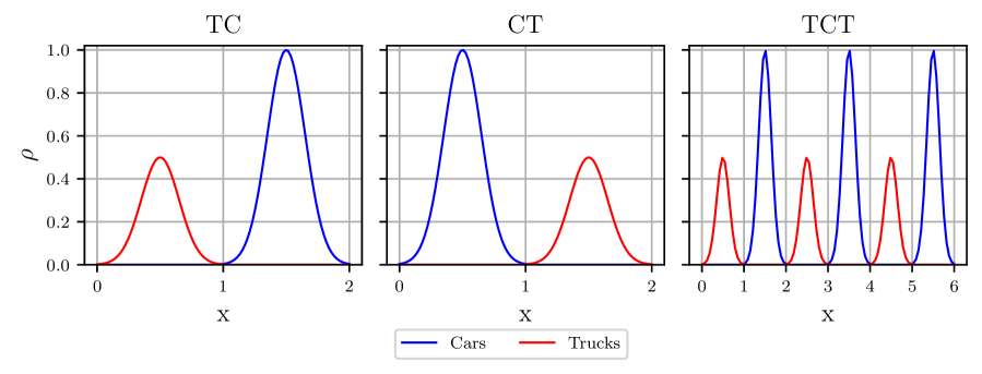
Figure 1: Two-class initial density configurations: TC is a fully segregated configuration with cars in front. CT is a fully segregated configuration with trucks in front. TCT is an interlaced configuration with alternating trucks and cars.

• Case 1: TC configuration. Fully segregated with cars in front with $\alpha_{1}=\alpha_{2}=1$. Then $L=L_{1}+L_{2}=2$, $\zeta_{0}^{1}(x)=\rho_{0,1}^{\left[1,2\right]}(x)$ and $\zeta_{0}^{2}(x)=\rho_{0,2}^{\left[0,1\right]}(x)$.

• Case 2: CT configuration. Fully segregated with trucks in front with $\alpha_{1}=\alpha_{2}=1$. Then $L=L_{1}+L_{2}=2$, $\zeta_{0}^{1}(x)=\rho_{0,1}^{\left[0,1\right]}(x)$ and $\zeta_{0}^{2}(x)=\rho_{0,2}^{\left[1,2\right]}(x)$.

• Case 3: TCT configuration. Interlaced configuration with $\alpha_{1}=\alpha_{2}=3$. Then $L=3L_{1}+3L_{2}=6$, $\zeta_{0}^{1}(x)=\rho_{0,1}^{\left[1,2\right]}(x)+\rho_{0,1}^{\left[3,4\right]}(x)+\rho_{0,1}^{\left[5,6\right]}(x)$ and $\zeta_{0}^{2}(x)=\rho_{0,2}^{\left[0,1\right]}(x)+\rho_{0,2}^{\left[2,3\right]}(x)+\rho_{0,2}^{\left[4,5\right]}(x)$.

where the $j$-th class’s initial density in $\left[x_{1},x_{2}\right]$ can be written as follow:

$$\rho_{0,j}^{\left[x_{1},x_{2}\right]}(x)=\rho_{j}^{a}+(\rho_{j}^{b}-\rho_{j}^{a})\cdot exp\left[-\frac{\left(x-\theta\right)^{2}}{2\gamma^{2}}\right]\cdot\mathbbm{1}_{\left[x_{1},x_{2}\right]}(x)$$ (31)

with $\rho_{1}^{a}=\rho_{2}^{a}=0.0$, $\rho_{1}^{b}=1.0$, $\rho_{2}^{b}=0.5$, $\gamma=0.15$ and $\theta=\frac{x_{1}+x_{2}}{2}$.

We refer to the three cases 1, 2, and 3, respectively, as TC, CT, and TCT in the presented figures.

Cost function 1: Generalized LWR.
We consider a generalization of the Lighthill-Whitham-Richards, referred to in all what follows as [GLWR], for $n$-population model introduced in [11], where the speed of each class is influenced by the presence of the others, thus:

$$u^{j}=U_{j}(\rho^{1},\rho^{2}),\text{for }j=1,2$$

.
We consider the general Greenshields-type speed-density:

$$U_{j}(\rho^{1},\rho^{2})=u_{max}^{j}(1-s)$$ (32)

with $s$ denoting the fraction of road occupancy ($0\leq s\leq 1$), defined as follow:

$$s=\rho^{1}l_{1}+\rho^{2}l_{2}$$ (33)

In other words, using (1), and taking into consideration that $L_{1}=L_{2}=1$:

$$s=\frac{\rho^{1}}{\rho^{1}_{jam}}+\frac{\rho^{2}}{\rho^{2}_{jam}}$$ (34)

Following the same lines as in the one-class case, we consider the cost function presented in [18], which consists of keeping the actual speed of vehicles $u_{j}$ not too far from the desired one in (32). Hence:

$$f_{j}^{\text{GLWR}}(u^{j},\rho^{1},\rho^{2})=\frac{1}{2}(U_{j}(\rho^{1},\rho^{2})-u^{j})^{2}$$ (35)

For [GLWR], the obtained density, speed, and optimal cost profiles for all scenarios, as shown in Figure 2 are qualitatively similar to those resulting from the single-class [LWR] model presented in [18] and reproduced in Figure 8.

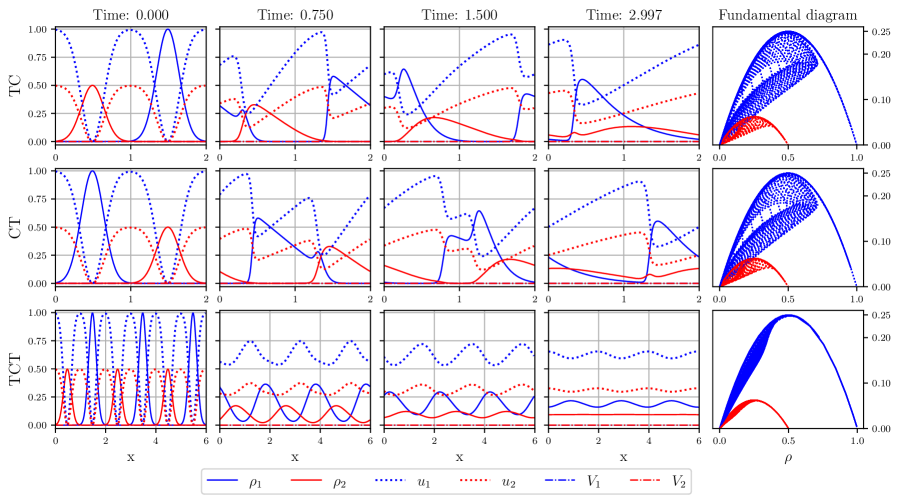
Figure 2: Cost function [GLWR]: evolution of density $\rho$, speed $u$, and optimal cost $V$ for cars and trucks, w.r.t. the position $x$. Each of the first four columns represents a time value, and the last column corresponds to the fundamental diagram. The rows represent the three cases TC, CT, and TCT.

When cars and trucks are fully segregated (TC and CT) as shown in Figure 2, we see that at some point they can manage to speed up and spread out their density around the mean. However, once one class reaches the other, we clearly observe a shock wave starting (Time: $0.75$), where the density before the shock point starts to increase. The shock is followed by a rarefaction along which the density after the shock point decreases. Because of the periodicity, the shock waves never disappear and are transported over time forming clusters of slow-moving vehicles, as shown at Time: $1.5$ and Time: $2.997$.

In the interlaced configuration (TCT), as shown in Figure 2, the traffic behavior is smoother. Indeed, no shock waves appear, and the density of both cars and trucks keeps spreading out over time. Although the correlation between the distribution of vehicles and the occurrence of shock waves is not clear, TCT experiment shows that a greater mixture can attenuate the formation of shock waves. This can be useful for traffic management, since more alternating distribution of vehicles is less likely to form clusters of slow-moving vehicles.

We observe in the fundamental diagrams of Figure 2 that for all [GLWR] cases, three different regimes are distinguished: In the free-flow regime, vehicles of both classes are in the free-flow ($\rho_{1}\leq 0.25$ and $\rho_{2}\leq 0.25$). In the semi-congested regime, the trucks’ class does not have enough space to maintain free flow, but the cars’ class still does ($\rho_{1}\leq 0.5$ and $\rho_{2}\geq 0.25$). In the fully-congested regime, both classes do not have sufficient space to maintain the free-flow speed ($\rho_{1}>0.5$ and $\rho_{2}>0.5$). In TC and CT configurations, most of the vehicles move to the semi-congested regime, which explains the formation of shock waves, unlike the TCT configuration, where most of the vehicles stay in the free-flow regime. But in the three configurations, only cars move to the fully-congested regime.

Another important observed result for [GLWR] is that the fundamental relation satisfies all important requirements for the classical generalized LWR model in every class. For $j=1,2$:

• Req1: Speed range $0\leq v_{j}\leq v_{max}^{j}$

• Req2: Density range $0\leq\rho_{j}\leq\rho_{jam}^{j}$

• Req3: No vehicle on the road $v_{j}=v_{max}^{j}$ when $\rho_{1}=\rho_{2}=0$

• Req4: Traffic jam $v_{j}=0$ when $\rho_{j}=\rho_{jam}^{j}$

• Req5: The fundamental diagram is strictly concave.

Req3 accounts for the fact that here, the flow depends not only on density, as in one class case, but also on the composition of the traffic.

Cost function 2: Generalized Separable.
We consider a generalization of the Separable cost function for one-class traffic proposed in [18], referred to in all what follows as [GS], defined by:

$$f_{j}^{\text{GS}}(u^{j},\rho^{1},\rho^{2})=\frac{1}{2}\left(\frac{u^{j}}{u^{j}_{max}}\right)^{2}-\frac{u^{j}}{u^{j}_{max}}+\frac{\rho}{\rho_{jam}}$$ (36)

where,

$$\left\{\begin{matrix}\rho=\rho^{1}l_{1}+\rho^{2}l_{2}\\ \rho_{jam}=\rho^{1}_{jam}l_{1}+\rho^{2}_{jam}l_{2}\end{matrix}\right.$$

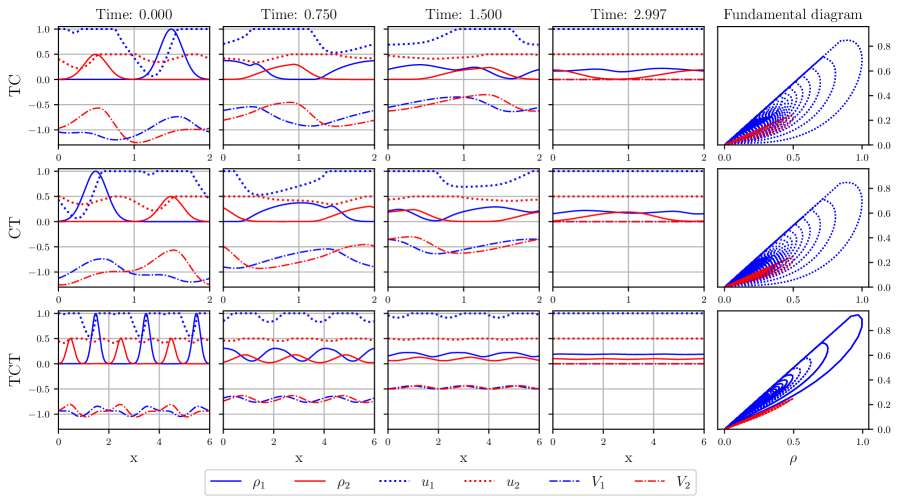
Figure 3: Cost function [GS]: evolution of density $\rho$, speed $u$, and optimal cost $V$ for cars and trucks, w.r.t. the position $x$. Each of the first four columns represents a time value, and the last column corresponds to the fundamental diagram. The rows represent the three cases TC, CT, and TCT.

Using (1), we get:

$$\left\{\begin{matrix}\rho=\frac{\rho^{1}}{\rho^{1}_{jam}}+\frac{\rho^{2}}{\rho^{2}_{jam}}\\ \rho_{jam}=2\end{matrix}\right.$$ (37)

Then (36) becomes:

$$f_{j}^{\text{GS}}(u^{j},\rho^{1},\rho^{2})=\frac{1}{2}\left(\frac{u^{j}}{u^{j}_{max}}\right)^{2}-\frac{u^{j}}{u^{j}_{max}}+\frac{1}{2}\left(\frac{\rho^{1}}{\rho^{1}_{jam}}+\frac{\rho^{2}}{\rho^{2}_{jam}}\right)$$ (38)

Cost function 3: Generalized Non-Separable.
We consider now a generalization of the Non-Separable cost function for one-class traffic proposed in [18], referred to in all what follows as [GNS] defined by:

$$f_{j}^{\text{GNS}}(u^{j},\rho^{1},\rho^{2})=\frac{1}{2}\left(\frac{u^{j}}{u^{j}_{max}}\right)^{2}-\frac{u^{j}}{u^{j}_{max}}+\frac{u^{j}}{u^{j}_{max}}\frac{\rho}{\rho_{jam}}$$ (39)

Using (37), the cost (39) becomes:

$$f_{j}^{\text{GNS}}(u^{j},\rho^{1},\rho^{2})=\frac{1}{2}\left(\frac{u^{j}}{u^{j}_{max}}\right)^{2}-\frac{u^{j}}{u^{j}_{max}}+\frac{1}{2}\frac{u^{j}}{u^{j}_{max}}\left(\frac{\rho^{1}}{\rho^{1}_{jam}}+\frac{\rho^{2}}{\rho^{2}_{jam}}\right)$$ (40)

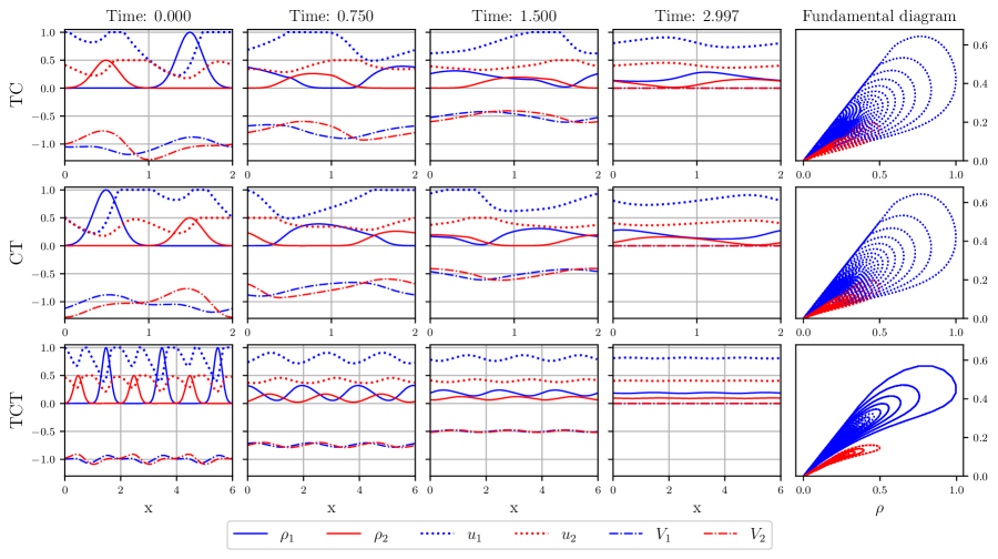
Figure 4: Cost function [GNS]: evolution of density $\rho$, speed $u$, and optimal cost $V$ for cars and trucks, w.r.t. the position $x$. Each of the first four columns represents a time value, and the last column corresponds to the fundamental diagram. The rows represent the three cases TC, CT, and TCT.

For [GS] in Figure 3, and [GNS] in Figure 4, there is no shock formation, thanks to the third term in the cost functions (38) and (40) that takes into account the level of density area as well as the composition of traffic. We observe the anticipation behavior in which the vehicles favor driving at a lower speed than the desired one, even in a low-density area, if there is a traffic jam ahead, contrary to [GLWR], where vehicles try to get as close as possible to the desired speed without anticipating the capacity of the road. As a result, the vehicles in [GLWR] are more sensitive to the changes in density, which clearly appears in the fundamental diagram of Figure 2 where we have steeper curves indicating that their flows are strongly impacted by density evolution. This information can help to identify the vehicles’ behaviors that are contributing most to congestion and to design targeted strategies that can be useful for congestion mitigation.

In both [GS] and [GNS], there is no fully-congested regime. Instead, a synchronized free-flow regime appears at Time: $2.997$, where vehicles of the same class move at a constant maximum speed and with uniform distribution, resulting in a smooth flow of traffic. Hence, the special closed shape of the fundamental diagrams in Figure 3, and Figure 4.

4.2 Microscopic discrete controls

In this section, we vary the number of vehicles in each class $(N_{j})_{j=1,2}$ such that $N_{j}=\alpha_{j}n$, with $n\in\left\{20,40,60,80,100\right\}$. Let $\alpha_{1}=\alpha_{2}=1$ for TC and CT, and $\alpha_{1}=\alpha_{2}=3$ for TCT.
We assume $L_{j}=n$, then $\rho_{jam}^{j}$ should fulfill (1), and $L=N_{1}+N_{2}$.
To reach the stable state at $T=3$, we consider the $j$-th class free flow speed $u_{max}^{j}\times L_{j}$.

Following the micro-macro approach introduced in Section 2.2, we first compute the NMFG-constructed controls from the macroscopic NMFG solutions by solving (16), using Algorithm 1.

Algorithm 1 NMFE-constructed controls

1:Given $N_{1}$ the number of cars and $N_{2}$ the number of trucks. $N=N_{1}+N_{2}$ the total number of vehicles. $(u_{1}^{*},u_{2}^{*})$ and $(\rho_{1}^{*},\rho_{2}^{*})$ the NMFE solutions.

2:Generate from the same initial densities used in macro-level $(\rho_{1}^{0},\rho_{2}^{0})$ : $N_{1}$ random samples for cars denoted $x_{1,0},...,x_{N_{1},0}$, and $N_{2}$ random samples for trucks denoted $x_{N_{1}+1,0},...,x_{N,0}$.

3:Compute the NMFE-constructed controls $\left\{\hat{v}_{i_{j}}(t)\right\}_{i_{j}\in\mathcal{I}_{j},j=1,2}$ using (16).

4:Compute the best response strategies $\left\{\bar{v}_{i_{j}}(t)\right\}_{i_{j}\in\mathcal{I}_{j},j=1,2}$ using algorithm 2.

5:Compute the accuracy associated $\left\{\hat{\varepsilon}_{i_{j}}\right\}_{i_{j}\in\mathcal{I}_{j},j=1,2}$ using (18).

6:Compute the maximum and mean accuracy :

$$\left\{\begin{matrix}\text{MaxRA}=\frac{\underset{j=1,2}{max}\left\{\underset{i_{j}\in\mathcal{I}_{j}}{max}\left|\hat{\varepsilon}_{i_{j}}\right|\right\}}{\underset{j=1,2}{max}\left\{\underset{i_{j}\in\mathcal{I}_{j}}{max}\left|J^{N}_{i_{j}}(\hat{v}_{i_{j}},\hat{v}_{-i_{j}},\hat{v}^{-j})\right|\right\}}\\ \text{MeanRA}=\frac{\sum_{j=1,2}\sum_{i_{j}\in\mathcal{I}_{j}}\left|\hat{\varepsilon}_{i_{j}}\right|}{\sum_{j=1,2}\sum_{i_{j}\in\mathcal{I}_{j}}\left|J^{N}_{i_{j}}(\hat{v}_{i_{j}},\hat{v}_{-i_{j}},\hat{v}^{-j})\right|}\end{matrix}\right.$$

We then compare them with the best response strategies computed by solving equations (19)-(20), using Algorithm 2.

Algorithm 2 Best response strategy

1:for $j:1,2$ do

2:     for $i_{j}\in\mathcal{I}_{j}$ do

3:         Initialize $k=0$, and choose a fixed line search step $\tau>0$ and a convergence tolerance $\epsilon<<1$.

4:         Choose $v_{i_{j}}^{(0)}(t)\in\left[0,1\right]$ (e.g, $v_{i_{j}}^{(0)}(t)=\frac{\hat{v}_{i_{j}}(t)}{u^{j}_{max}\times L_{j}}$).

5:         for $m\in\mathcal{I}_{1}\cup\mathcal{I}_{2}$ do

6:              Solve the state equation (Explicit forward Euler) :

$$\left\{\begin{matrix}\dot{x}_{m}^{(k)}(t)=\left\{\begin{matrix}\hat{v}_{m}(t)/(u^{j}_{max}\times L_{j})&\text{if }m\neq i_{j}\\ v_{m}^{(k)}(t)/(u^{j}_{max}\times L_{j})&\text{if }m=i_{j}\\ \end{matrix}\right.\\ x_{m}^{(k)}(0)=x_{m,0}/L\end{matrix}\right.$$

         

7:         Solve the backward adjoint state equation (Explicit forward Euler) :

$$\left\{\begin{matrix}\dot{P}_{i_{j}}^{(k)}(t)=-\nabla_{x}f_{j}\left(v_{i_{j}}^{(k)}(t),\rho^{1}\left(t,x_{i_{j}}^{(k)}(t)\right),\rho^{2}\left(t,x_{i_{j}}^{(k)}(t)\right)\right)\\ P_{i_{j}}^{(k)}(T)=0\end{matrix}\right.$$

8:         Compute the gradient :

$$g_{i_{j}}^{(k)}(t)=P_{i_{j}}^{(k)}(t)+\nabla_{v}f_{j}\left(v_{i_{j}}^{(k)}(t),\rho^{1}\left(t,x_{i_{j}}^{(k)}(t)\right),\rho^{2}\left(t,x_{i_{j}}^{(k)}(t)\right)\right)$$

9:         if $\|g_{i_{j}}^{(k)}(t)\|\leq\epsilon$ then

10:              $v_{i_{j}}^{(k+1)}(t)=v_{i_{j}}^{(k)}(t)$

11:         else

12:              $v_{i_{j}}^{(k+1)}(t)=v_{i_{j}}^{(k)}(t)-\tau g_{i_{j}}^{(k)}(t)$          

13:         if $v_{i_{j}}^{(k+1)}(t)\approx v_{i_{j}}^{(k)}(t)$ then

14:              $\bar{v}_{i_{j}}(t)=v_{i_{j}}^{(k+1)}(t)\times u^{j}_{max}\times L_{j}$

15:         else

16:              $k=k+1$.

17:              Repeat from 4:               

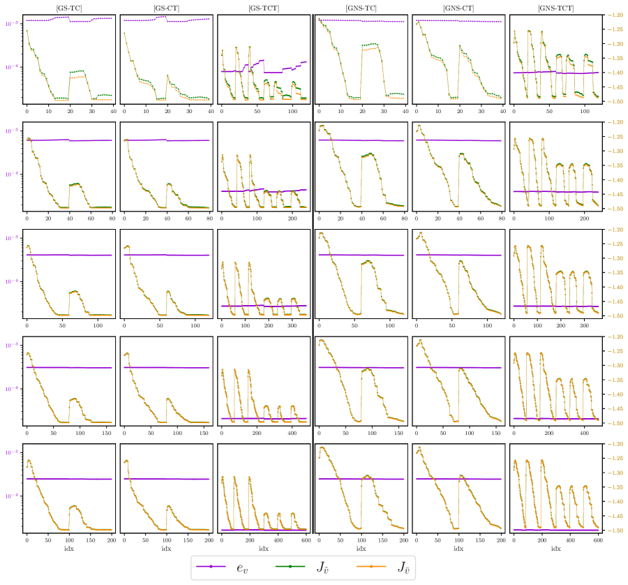
Figure 5: The columns correspond to the TC, CT, and TCT configurations, considering [GS] (left) and [GNS] (right). The rows are for different total number of vehicles $N$. Each sub-figure presents three curves: the $L_{\infty}$ norm $e_{v}=\left\|\hat{v}-\bar{v}\right\|_{\infty}$, the cost for NMFE-constructed controls $J_{\hat{v}}=J_{i_{j}}(\hat{v}_{i_{j}},\hat{v}_{-i_{j}},\hat{v}^{-j})$, and the cost for the best response strategies $J_{\bar{v}}=J_{i_{j}}(\bar{v}_{i_{j}},\hat{v}_{-i_{j}},\hat{v}^{-j})$, all w.r.t. vehicle’s index (idx).

From Figure 5, we notice the following results: the values of cost function when vehicles move with their NMFE-constructed controls $J_{\hat{v}}=J_{i_{j}}(\hat{v}_{i_{j}},\hat{v}_{-i_{j}},\hat{v}^{-j})$ are closer to those when vehicles move with their best response strategies $J_{\bar{v}}=J_{i_{j}}(\bar{v}_{i_{j}},\hat{v}_{-i_{j}},\hat{v}^{-j})$ which proves that the macro-macro approach provides a good approximation of the vehicles control and shows the relevance of the algorithms proposed. We observe that the $L_{\infty}$ norm of the difference between the NMFE-constructed controls $\hat{v}$ and the best response strategies $\bar{v}$ denoted by $e_{v}=\left\|\hat{v}-\bar{v}\right\|_{\infty}$ are small and decreases every time the total number of vehicles $N$ increases, which is consistent with the main idea of the mean-field theory.

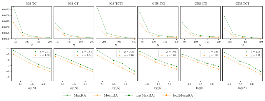
Figure 6: The columns correspond to the TC, CT, and TCT configurations, considering [GS] (left) and [GNS] (right). The first row represents the mean accuracy (MeanRA) and maximum accuracy (MaxRA) for different total number of vehicles $N$. The second row shows their respective log-log plots, with $-\mu$ and $-\eta$ being the slopes.

In Figure 6, we observe from the first row that when the total number of vehicles $N$ increases, the relative accuracy decreases; therefore, a better control approximation is obtained. Moving to the second row, where log-log plots are displayed for each configuration to analyze the relationship between the relative accuracies and $N$. We clearly observe that MaxRA and MeanRA behave as $N^{-\mu}$ and $N^{-\eta}$ respectively. The experimental results found for $\mu$ and $\eta$ are larger than $\frac{1}{4}$, the latter is what is expected by the theory, see [14] section 6.1 Theorem 6.7. The same behavior appears in the case of one-class in Figure 10.

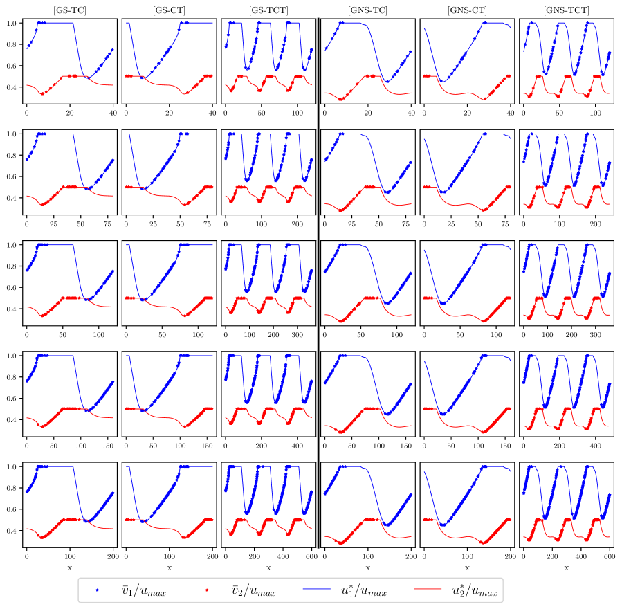
Figure 7: The columns correspond to the TC, CT, and TCT configurations, considering [GS] (left) and [GNS] (right). The rows are for different total number of vehicles $N$. Each sub-figure presents: the relative macro NMFE $u^{*}_{j}/u_{max}$ and the relative best controls $\bar{v}_{j}/u_{max}$ at $t=0.6$, for cars (j=1) and trucks (j=2).

Figure 7 shows the anticipation behavior of vehicles on the microscopic scale for [GS] and [GNS], which is consistent with what is described on the macroscopic scale in Figure 3 and Figure 4.

5 Conclusion

In this paper, we have explored a multi-class traffic model and examined the computational feasibility of mean-field games (MFG) in obtaining approximate Nash equilibria for traffic flow games involving a large number of players. We introduced a two-class traffic framework, building upon the ideas presented in the single-class approach by [18]. To facilitate our analysis, we employed various numerical techniques, including high-performance computing and regularization of LGMRES solvers. By utilizing these tools, we conducted simulations at significantly larger spatial and temporal scales.

We led extensive numerical experiments considering three different scenarios involving cars and trucks, as well as three different cost functionals. Our results primarily focused on the dynamics of autonomous vehicles (AVs) in traffic, which support the effectiveness of the approach proposed by [18].

Moreover, we conducted original comparisons between macroscopic Nash mean-field speeds and their microscopic counterparts. These comparisons allowed us to computationally validate the $\epsilon-$Nash approximation, demonstrating a slightly improved convergence rate compared to theoretical expectations.

Future directions encompass second order traffic models, the multi-lane case, particularly prone to non-cooperative game considerations, and addressing some theoretical issues.

Actually, first-order models have severe limitations in describing important traffic features, such as light traffic with slow drivers and stop-and-start transitions. The first second-order model was introduced in [26], which at its turn was criticized in [15] for it violates critical traffic principles such as that cars react to front stimuli (and not to cars behind). The model was "resurrected" later in [6, 29]. However, the game version of the model has not yet been explored. Moreover, this work may be extended to handle the case where the traffic flow is on a multi-lane road, for which non-game model versions are proposed on both microscopic and macroscopic scales. See for example [28, 25]. Finally, numerous theoretical issues arising from the two-class modeling, such as existence of solutions to the generalized limit systems (e.g. generalized LWR and generalized separable systems) or convergence properties of the discretized nonlinear systems.

Acknowledgements: This work was supported in part by using the resources of Mohammed VI Polytechnic University through Simlab & Toubkal the HPC & IA platforms.

Appendix A One-class traffic

For one class of traffic model proposed in [18], we plot in Figure 8 the evolution of the density, the velocity field, and the optimal control, as well as the fundamental diagram for the three examples of the cost functions [LWR], [Separable], and [Non-Separable].

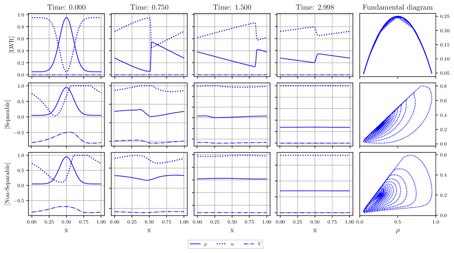
Figure 8: One-class (cars): Evolution of density $\rho$, speed $u$, and optimal cost $V$ in four-time values (four columns). The rows show the three cost functions [LWR], [Separable], and [Non-Separable]. The last column shows the fundamental diagram.

Figure 9 shows the $L_{\infty}$ norm $e_{v}=\left\|\hat{v}-\bar{v}\right\|_{\infty}$. The cost function when cars move with their NMFE-constructed controls $J_{\hat{v}}=J_{i_{1}}(\hat{v}_{i_{1}},\hat{v}_{-i_{1}})$, and the cost when cars move with their best response strategies $J_{\bar{v}}=J_{i_{1}}(\bar{v}_{i_{1}},\hat{v}_{-i_{1}})$.

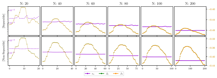
Figure 9: The columns represent the different total number of cars $N$. The rows correspond to the [Separable] and [Non-separable] cost functions. Each sub-figure shows three curves: the $L_{\infty}$ norm $e_{v}=\left\|\hat{v}-\bar{v}\right\|_{\infty}$, the cost for NMFE-constructed controls $J_{\hat{v}}=J_{i_{1}}(\hat{v}_{i_{1}},\hat{v}_{-i_{1}})$, and the cost for the best response strategies $J_{\bar{v}}=J_{i_{1}}(\bar{v}_{i_{1}},\hat{v}_{-i_{1}})$, all w.r.t. car’s index (idx).

In Figure 10 we plot in the first row the mean accuracy (MeanRA) and maximum accuracy (MaxRA) with respect to the number of the cars, and in the second row their respective log-log plots.

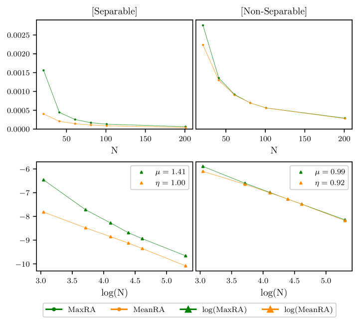
Figure 10: The columns correspond to the [Separable] and [Non-separable] cost functions. The first row shows the mean accuracy (MeanRA) and maximum accuracy (MaxRA) for different total number of cars $N$. The second row shows their respective log-log plots, with $-\mu$ and $-\eta$ being the slopes.

References

- [1] Shrirang Abhyankar et al. “PETSc/TS: A modern scalable ODE/DAE solver library” In arXiv preprint arXiv:1806.01437, 2018
- [2] Y. Achdou et al. “Hamilton-Jacobi Equations: Approximations, Numerical Analysis and Applications: Cetraro, Italy 2011, Editors: Paola Loreti, Nicoletta Anna Tchou”, Lecture Notes in Mathematics Springer Berlin Heidelberg, 2013 URL: https://books.google.co.ma/books?id=MiS6BQAAQBAJ
- [3] Yves Achdou, Fabio Camilli and Italo Capuzzo Dolcetta “Mean Field Games: Numerical Methods for the Planning Problem” In SIAM J. Control. Optim. 50, 2012, pp. 77–109
- [4] Yves Achdou and Ziad Kobeissi “Mean Field Games of Controls: Finite Difference Approximations” In ArXiv abs/2003.03968, 2020
- [5] Yves Achdou and Mathieu Laurière “Mean field games and applications: Numerical aspects” In Mean field games Springer, 2020, pp. 249–307
- [6] A. Aw and M. Rascle “Resurrection of "Second Order" Models of Traffic Flow” In SIAM Journal on Applied Mathematics 60.3, 2000, pp. 916–938 DOI: 10.1137/S0036139997332099
- [7] AH Baker, ER Jessup and T Manteuffel “A technique for accelerating the convergence of restarted GMRES” In SIAM Journal on Matrix Analysis and Applications 26.4, 2005, pp. 962–984
- [8] Satish Balay et al. “PETSc users manual”, 2019
- [9] Satish Balay et al. “PETSc Web page”, https://petsc.org/, 2022 URL: https://petsc.org/
- [10] Alain Bensoussan, Tao Huang and Mathieu Lauriere “Mean Field Control and Mean Field Game Models with Several Populations” In Minimax Theory and its Applications 3.2, SI, 2018, pp. 173–209
- [11] Sylvie Benzoni-Gavage and Rinaldo M. Colombo “An n-populations model for traffic flow” In Europ. J. Appl.Math 14.5, 2003, pp. 587–612
- [12] Emily Bourne, Yaman Güçlü, Said Hadjout and Ahmed Ratnani “Pyccel: a Python-to-X transpiler for scientific high-performance computing” In Journal of Open Source Software 8.83, 2023, pp. 4991
- [13] René A. Carmona and François Delarue “Probabilistic Analysis of Mean-Field Games” In SIAM J. Control. Optim. 51, 2012, pp. 2705–2734
- [14] René Carmona and François Delarue “Probabilistic Theory of Mean Field Games with Applications II Mean Field Games with Common Noise and Master Equations” Springer, 2018
- [15] Carlos F. Daganzo “Requiem for second-order fluid approximations of traffic flow” In Transportation Research Part B: Methodological 29.4, 1995, pp. 277–286 DOI: 10.1016/0191-2615(95)00007-Z
- [16] Lisandro Dalcin and Yao-Lung L. Fang “mpi4py: Status Update After 12 Years of Development” In Computing in Science & Engineering 23, 2021, pp. 47–54
- [17] Serge P Hoogendoorn and Piet HL Bovy “State-of-the-art of vehicular traffic flow modelling” In Proceedings of the Institution of Mechanical Engineers, Part I: Journal of Systems and Control Engineering 215.4 SAGE Publications Sage UK: London, England, 2001, pp. 283–303
- [18] Kuang Huang, Xuan Di, Qiang Du and Xi Chen “A Game-Theoretic Framework for Autonomous Vehicles Velocity Control: Bridging Microscopic Differential Games and Macroscopic Mean Field Games” In Discrete and Continuous Dynamical Systems-Series B 25.12, 2020, pp. 4869–4903
- [19] Minyi Huang, Roland P. Malhamé and Peter E. Caines “Large population stochastic dynamic games: Closed-loop McKean-Vlasov systems and the Nash certainty equivalence principle” In Communications in Information & Systems 6.3, 2006, pp. 221 –252
- [20] Dana Knoll and David Keyes “Jacobian-free Newton-Krylov methods: a survey of approaches and applications” In Journal of Computational Physics 193.2, 2004, pp. 357–397
- [21] Jean-Michel Lasry and Pierre-Louis Lions “Mean field games” In Japanese Journal of Mathematics 2.1, 2007, pp. 229–260
- [22] Nicolas Laurent-Brouty et al. “Information Patterns in the Modeling and Design of Mobility Management Services” In Proceeding of the IEEE 106.4, SI, 2018, pp. 554–576
- [23] Mathieu Lauriere “Numerical Methods for Mean Field Games and Mean Field Type Control” In arXiv:2106.06231 [cs, math], 2021
- [24] RM Lewis and SG Nash “Model problems for the multigrid optimization of systems governed by differential equations” In SIAM Journal on Scientific Computing 26.6, 2005, pp. 1811–1837
- [25] Hari Hara Sharan Nagalur Subraveti, Victor L Knoop and Bart Arem “First order multi-lane traffic flow model–an incentive based macroscopic model to represent lane change dynamics” In Transportmetrica B: Transport Dynamics 7.1 Taylor & Francis, 2019, pp. 1758–1779
- [26] Harold J Payne “Model of freeway traffic and control” In Mathematical Model of Public System, 1971, pp. 51–61
- [27] Stanisław Węglarczyk “Kernel density estimation and its application” In ITM Web of Conferences 23, 2018, pp. 00037 EDP Sciences
- [28] Qi Yang and Koutsopoulos H. N. “A microscopic traffic simulator for evaluation of dynamic traffic management systems” In Transportation Research Part C: Emerging Technology 4(3), 1996, pp. 113–129
- [29] H. M. Zhang “A non-equilibrium traffic model devoid of gas-like behavior” In Transportation Research Part B: Methodological 36.3, 2002, pp. 275–290 DOI: 10.1016/S0191-2615(00)00050-3